Hopf Bifurcation and Phase Patterns
in Symmetric Ring Networks

Abstract

Systems of ODEs coupled with the topology of a closed ring are common models in biology, robotics, electrical engineering, and many other areas of science. When the component systems and couplings are identical, the system has a cyclic symmetry group for unidirectional rings and a dihedral symmetry group for bidirectional rings. Hopf bifurcation in equivariant and network dynamics predicts the generic occurrence of periodic discrete rotating waves whose phase patterns are determined by the symmetry group. We review basic aspects of the theory in some detail and derive general properties of such rings. New results are obtained characterising the first bifurcation for long-range couplings and the direction in which discrete rotating wave states rotate.

1 Introduction

Oscillatory processes, in which the same behaviour repeats periodically as time passes, are widespread in the natural world. Examples in the life sciences include the motion of animals [13, 44, 46, 71], breathing [4], the heartbeat [68], peristalsis in the gut [30, 56], the sleep-wake cycle [10], networks of neurons [9, 12, 23, 29, 31, 48, 57, 62, 67, 69, 75], gene regulatory networks [14, 24], and biological development [76]. Such processes have been modelled extensively as networks of oscillators [5, 11, 25, 26, 51, 52, 53, 63, 64, 66, 78, 79]. The term ‘oscillator’ tacitly assumes that the component subsystems must be capable of sustaining oscillatory dynamics in isolation. We do not make this assumption, which is not necessary for most networks, so we refer to these subsystems as nodes.

Similar periodic patterns also arise in the physical sciences, for instance robotics [49, 50], electronic engineering [27, 55, 21], Josephson junction arrays [8], and celestial mechanics [58, 61, 72]. Often the model equations are based on detailed features of the underlying physics; for example planetary orbits are modelled using Newton’s laws of gravity and motion. The equations can also be simplified ‘toy’ models that illustrate mathematical features of the physics, such as the ‘kicked oscillator’ model for Arnold tongues in resonance [45].

A feature of some of these models is the occurrence of phase patterns, in which distinct nodes have the same time-periodic waveform subject to a phase shift. Often these phase shifts are simple fractions of the period, regularly spaced round the ring. We call such a state a discrete rotating wave, or a standing wave when all oscillators are synchronised. Other terms in the literature are rosette [48] and ponies on a merry-go-round [8]. We discuss the relation between phase patterns and symmetries of the equations using equivariant and network dynamics and bifurcation theory.

Hopf Bifurcation

In this paper we consider networks of coupled continuous-time dynamical systems (ordinary differential equations, ODEs). For simplicity we restrict to state variables in real vector spaces, but much of the theory extends to manifolds [2, 3, 19].

Periodic oscillations in a dynamical system can arise through a variety of mechanisms. A common one is Hopf bifurcation, in which an equilibrium loses stability as some parameter varies, generating a limit cycle. A necessary condition is that the linearised equation has nonzero purely imaginary eigenvalues $\pm\mathrm{i}\omega$, where $0\neq\omega\in\mathbb{R}$. Such eigenvalues are said to be critical. With additional ‘nondegeneracy’ conditions (simplicity of this eigenvalue, no other imaginary eigenvalues, and the ‘eigenvalue crossing’ condition) the Hopf Bifurcation Theorem guarantees the existence of a unique bifurcating branch of periodic solutions [47]. These conditions are generic in general dynamical systems, but not for symmetric dynamical systems [42] or those with network structure [39]. Nonetheless, useful analogues of the Hopf Bifurcation Theorem hold in these contexts. We therefore employ the term ‘Hopf bifurcation’ in a loose sense: the occurrence of purely imaginary critical eigenvalues. In this paper we focus on oscillations generated by Hopf bifurcation in this sense.

Phase Patterns

A network system has distinguished observables, namely the states of its nodes, and these can be compared to each other. In many cases the oscillations exhibit clear patterns in which the phases of distinct component units are related in specific ways. Biological examples include quadruped gaits [13, 17, 18, 44, 46], such as the walk, in which the limbs typically move in the sequence

$$\mbox{left rear}\ \to\ \mbox{left front}\ \to\ \mbox{right rear}\ \to\ \mbox{right front}\ \to\cdots$$

and each limb moves one quarter of the period after the previous one. Figure 1 illustrates this pattern in the walk of an elephant.

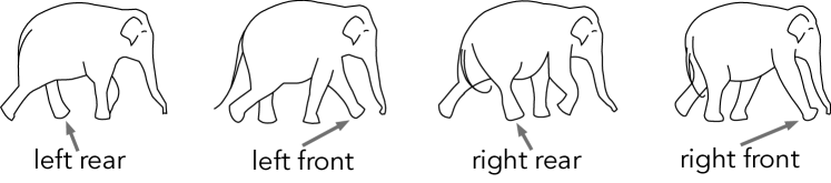
Figure 1: Walk of an elephant at $\frac{1}{4}$-period intervals.

Central configurations in celestial mechanics [58, 61, 72] are a physical example. Suppose that four identical point masses (planets) revolve round a central point mass (star), so that the planets follow a circular orbit in the plane and lie at the vertices of a uniformly rotating square. Such a state is consistent with Newtonian gravitation for a suitable choice of the mass and angular velocity. This state has the same spatiotemporal symmetries as the walk gait: successive planets follow identical orbits with a phase shift of one quarter of the period. Another example in this context is the occurrence of choreographies, such as three identical masses moving along the same figure-8 shaped orbit [15]. An important mathematical difference here is that the equations of celestial mechanics are Hamiltonian, but analogous results apply [59, 60]. Another is that the centre of mass remains stationary in central configurations; this happens because the gravitational forces acting on the star combine through vector addition, so they cancel out. Such cancellations are common when interactions are additive.

Networks and Ring Topology

A network of coupled ODEs is a directed graph in which each node corresponds to a component ODE, and each arrow (directed edge) indicates that the state of the node at the head of the arrow is influenced by that of the node at its tail [39, 43, 73]. In this paper we focus on dynamical systems in which several subsystems are coupled together with the topology or symmetry of a closed ring. Figure 2 illustrates the two main types of ring for identical components with identical nearest-neighbour (NN) coupling. We draw each node as a circle and each directed edge as an arrow, with double-headed arrows for bidirectional coupling. It is convenient to number nodes with integers $\{0,1,\ldots,n-1\}$ modulo $n$, where $n$ is the number of nodes and nodes are numbered consecutively in the anticlockwise direction.

Figure 2: Left: 5-node unidirectional ring. Right: 6-node bidirectional ring.

Symmetry Induces Phase Patterns

For suitable ODEs, unidirectional and bidirectional rings with identical nodes and arrows naturally sustain periodic oscillations such that the relative phases of consecutive nodes differ by the same fraction of the period. These patterns are a consequence of the symmetries of the ring: the permutations of nodes that preserve the connecting arrows [39, 42]. The symmetry group of an $n$-node unidirectional ring of identical nodes with identical NN coupling, as in Figure 2 (left), is the cyclic group $\mathbb{Z}_{n}$ of order $n$, which is isomorphic to the group of rotational symmetries of a regular $n$-gon. Considered as a permutation group acting on the nodes, $\mathbb{Z}_{n}$ is generated by the $n$-cycle $\alpha=(0\,1\,2\,\cdots\,n-1)$. The symmetry group of an $n$-node bidirectional ring (of identical nodes with identical NN coupling as in Figure 2(right)) is the dihedral group $\mathbb{D}_{n}$ of order $2n$, which is isomorphic to the group of rotational and reflectional symmetries of a regular $n$-gon. The group $\mathbb{D}_{n}$ is generated by $\alpha$ and the map $\kappa$ where $\kappa(j)=-j\pmod{n}$.

More generally, in Section 3.1 we discuss oscillations of ODEs with a symmetry group $\Gamma$. The main result here is the Equivariant Hopf Theorem, which proves the existence of bifurcating branches of solutions with certain spatiotemporal symmetries, under suitable conditions. When applied to ODEs with $n$-fold rotational symmetry $\mathbb{Z}_{n}$, this result shows that typical oscillation patterns created by Hopf bifurcation have phase shifts $kT/n$ between successive nodes, where $T$ is the overall period and $0\leq k<n$ is an integer: the aforementioned discrete rotating waves. See Theorem 3.7. The predicted patterns for $\mathbb{D}_{n}$ symmetry are more complicated; see Section 7 and [37, 38, 42].

In particular, the $\frac{1}{4}$-period phase pattern in Figure 1 can occur in a rigid manner in a unidirectional ring of four identical systems with identical coupling, which has symmetry group $\mathbb{Z}_{4}$. By ‘rigid’ we mean that the phase pattern, as a fraction of the period, persists after sufficiently small perturbations of the ODE that preserve the symmetry and network topology. This condition is a form of structural stability [74]. Such a ring can also support a phase pattern where the phase shift from one node to the next is $0,\mbox{\footnotesize$\frac{1}{2}$}$, or $\frac{3}{4}$ of the period, depending on the form of the ODE and the solution under consideration. For some ODEs, different patterns may coexist for different initial conditions. The stability of such states is a complicated issue, addressed in [36, 37, 42] using Birkhoff normal form reduction.

Remarks 1.1.

(a) Although $\mathbb{Z}_{4}$ symmetry generates the phase pattern of the walk gait, a network that can generate all of the main quadruped gaits, without distinct gaits being stable simultaneously, has at least 8 nodes and $\mathbb{Z}_{2}\times\mathbb{Z}_{4}$ symmetry [40, 41].

(b) Other examples of regular phase patterns include oscillations of the repressilator, a synthetic genetic circuit [24], and a ring of three identical FitzHugh–Nagumo neurons [39]. Both systems are modelled by ODEs with $\mathbb{Z}_{3}$ symmetry, and Hopf bifurcation gives rise to oscillations in which successive components are related by phase shifts of one third of the period.

(c) In generic $\mathbb{Z}_{n}$-symmetric Hopf bifurcation, critical eigenvalues are simple and the classical Hopf Bifurcation Theorem applies. However, the Equivariant Hopf Theorem provides extra information on the spatiotemporal symmetries of the oscillations. These symmetries are present in the linearised eigenfunctions, that is, in the form of the critical eigenvectors, which proves that the phase pattern exists at linear order. However, the Equivariant Hopf Theorem shows that the pattern is exact, even when nonlinear (symmetric) terms are present.

(d) In the network context, the situation is not so straightforward. Equivariant maps for a network with symmetry group $\Gamma$ need not be admissible. In consequence the basic theorem that generically the critical eigenspace for an imaginary eigenvalue is $\Gamma$-simple is no longer valid. The reason is that the proof of this theorem involves linear perturbations given by projection to irreducible components, which may not be admissible. However, for the $\mathbb{Z}_{n}$-symmetric ring networks studied in this paper, it can be proved directly that all eigenvalues of generically simple.

1.1 Summary of Paper

Section 2 summarises required background material on local bifurcation, with emphasis on Hopf bifurcation. It discusses the role of symmetry in dynamics through the notion of an equivariant ordinary differential equation (ODE).

Section 3 introduces the main concepts involved in equivariant dynamics and the analogous theory for network dynamics. In particular we define the class of admissible ODEs associated with any network; these are the ODEs that respect the network topology in a specific formal sense. We review key results from the representation theory of compact Lie groups, and in particular finite groups, and explain how they apply to local bifurcation in equivariant dynamical systems. We discuss symmetry-breaking and state the Equivariant Hopf Theorem on the existence of bifurcating branches of periodic states for certain groups of spatio-temporal symmetries. We also mention time reversal symmetry.

Section 4 applies the Equivariant Hopf Theorem to unidirectional ring networks with cyclic symmetry group $\mathbb{Z}_{n}$. The analysis leads to conditions for the existence of discrete rotating waves, in which successive nodes in the ring oscillate with the same waveform but regularly spaced phases $\frac{kT}{n}$ where $T$ is the overall period and $k$ is an integer between 0 and $n-1$. Assuming nodes have 1-dimensional state spaces $\mathbb{R}$, the first bifurcation—the only one that can be stable locally—is Hopf if and only if the number $n=2N+1$ of nodes is odd. The associated phase shifts are then $\frac{NT}{2N+1}$ or $\frac{(N+1)T}{2N+1}$.

Section 5 specialises the results to networks. We study Hopf bifurcation in a unidirectional ring with nearest neighbour coupling. Again we assume nodes have 1-dimensional state spaces $\mathbb{R}$. We begin with nearest-neighbour coupling, in which case the results of Section 5 impose constraints on the phase shift for the first Hopf bifurcation. We show that when longer-range couplings are allowed, the different types of Hopf bifurcation can occur in any order.

Section 6 generalises the analysis to nodes with higher-dimensional state spaces. We show by example that the strong constraints on the first bifurcation no longer apply.

Section 7 carries out similar analyses for bidirectional rings, with symmetry group $\mathbb{D}_{n}$. We also mention ‘exotic’ synchrony and phase patterns in networks, which arise for combinatorial reasons rather than being associated with symmetries, and discuss the difference between equivariant and admissible ODEs.

2 Background on Dynamics and Bifurcations

We assume familiarity with basic concepts in nonlinear dynamics and bifurcation theory; see [45]. In particular we assume knowledge of the classical Hopf Bifurcation Theorem on the transition from a stable equilbrium to a branch of periodic states [47]. We summarise analogous concepts for equivariant dynamics [42] and network dynamics [39, 43, 73].

2.1 Local Bifurcation

Consider a 1-parameter family of smooth ($C^{\infty}$) maps $f:\mathbb{R}^{n}\times\mathbb{R}\rightarrow\mathbb{R}^{n}$, where $\lambda\in\mathbb{R}$ is a parameter. There is a corresponding family of ODEs:

$$\dot{x}=f(x,\lambda)\qquad x\in\mathbb{R}^{n},\lambda\in\mathbb{R}$$ (1)

For simplicity in stating results, we assume that for each $\lambda$, solutions $x_{\lambda}(t)$ for given initial conditions $x_{\lambda}(0)$ exist for all $t\in\mathbb{R}$. This condition is generically valid [54]. Usually all we need is local existence for $t$ near $0$, which holds for all smooth $f$. More technically, everything can be stated for $t$ lying in a suitable interval.

A branch is a parametrised family $\{x_{\lambda}(t)\}$ of solutions that vary continuously with $\lambda$. A local bifurcation occurs at $(x_{0},\lambda_{0})$ if the topology of the set of solutions is not constant near $(x_{\lambda_{0}}(x_{0}),\lambda_{0})$. There are two types of local bifurcation: steady-state and Hopf.

A necessary condition for the occurrence of local bifurcation from a branch of equilibria at $(x_{0},\lambda_{0})$ is that the Jacobian (or derivative) $J=\mathrm{D}f|_{x_{0},\lambda_{0}}$ should have eigenvalues on the imaginary axis (including 0). These are the critical eigenvalues and their real eigenspaces are the critical eigenspaces. (The real eigenspace $E_{\mu}$ for a non-real eigenvalue $\mu$ is the real part of the sum of the complex eigenspaces for $\mu$ and its conjugate $\bar{\mu}$. It is spanned over $\mathbb{R}$ by the real and imaginary parts of the complex eigenvectors.)

(1)  A zero eigenvalue usually corresponds to steady-state bifurcation: typically, the number of equilibria changes near $(x_{0},\lambda_{0})$, and branches of equilibria may appear, disappear, merge, or split as $\lambda$ varies near $\lambda_{0}$. The possibilities here can be organised, recognised, and classified using singularity theory [42].

(2)  A nonzero imaginary eigenvalue usually corresponds to Hopf bifurcation [45, 47]. Under suitable genericity conditions(a simple pair of eigenvalues $\pm\mathrm{i}\omega$, no other imaginary eigenvalues, and the eigenvalue crossing condition) this leads to periodic solutions whose amplitude (near the bifurcation point) is small. Degenerate Hopf bifurcation, where the eigenvalue crossing condition fails, has been analysed using singularity theory [32].

Normalised Period and Phase Shifts

Suppose that $\rho(t)$ is a $T$-periodic function. Define the corresponding circle group to be ${\bf S}^{1}=\mathbb{R}/T\mathbb{Z}$. This is the group of phase shifts of $\rho$ modulo the period. It is isomorphic to the multiplicative group of complex numbers ${\mathrm{e}}^{\mathrm{i}\theta}$ on the unit circle by the map ${\mathrm{e}}^{\mathrm{i}\theta}\mapsto\frac{T\theta}{2\pi}$, and we often use this isomorphism to identify the two groups.

There are two main conventions when defining a phase shift, differing in sign. We adopt the following convention:

Definition 2.1.

Let $\rho(t)$ be a $T$-periodic function and let $\theta\in{\bf S}^{1}=\mathbb{R}/T\mathbb{Z}$. Then

$$\rho(t-\theta)$$ (2)

is $\rho(t)$ phase-shifted by $\theta$. Also, $\theta$ is the phase shift from $\rho(t)$ to $\rho(t-\theta)$. To obtain a unique value it is convenient to normalise $\theta$ to lie in $[0,T)$.

For fixed $\theta$ and variable $t$, the time series of $\rho(t-\theta)$ is that of $\rho(t)$ shifted $\theta$ to the right. The alternative convention has a $+$ sign in (2). Now $\theta$ changes to $-\theta$ so the time series is shifted $\theta$ to the left.

For example, in the walk gait the movement of successive legs is separated by $\frac{1}{4}$-period phase shifts.

2.2 Symmetries

A symmetry of an ODE is a permutation $\sigma$ of the variables that preserves the ODE. A symmetry of a network is a permutation $\sigma$ of the nodes that preserves arrows and their types.

Example 2.2.

Consider the following ODE in variables $x=(x_{0},x_{1},x_{2})$:

$$\begin{array}[]{rcl}\dot{x}_{0}&=&\lambda x_{0}-x_{0}^{3}+ax_{2}\\ \dot{x}_{1}&=&\lambda x_{1}-x_{1}^{3}+ax_{0}\\ \dot{x}_{2}&=&\lambda x_{2}-x_{2}^{3}+ax_{1}\end{array}$$ (3)

where $\lambda$ acts as a bifurcation parameter and $a$ is a coupling strength.

Equation (3) is symmetric under the cyclic permutation $\alpha=(0\,1\,2)$. That is, if we apply $\alpha$ to the equations we obtain the same set of equations, though listed in permuted order. Abstractly, the equations are equivariant for the group $\Gamma=\mathbb{Z}_{3}$ generated by $\alpha$. This means that if we write the ODE as $\dot{x}=f(x)$, where $x=(x_{0},x_{1},x_{2})$ and $f=(f_{0},f_{1},f_{2})$, then

$$f(\gamma x)=\gamma f(x)\qquad\forall\gamma\in\Gamma$$ (4)

Here

$$\alpha x=(x_{1},x_{2},x_{0})\qquad\alpha f=(f_{1},f_{2},f_{0})$$

Because the functions involved are odd in $x$, equation (3) has a further symmetry $\kappa(x)=-x$, so the full symmetry group is $\mathbb{Z}_{3}\times\mathbb{Z}_{2}$. We discuss this later in Section 5.1. (Adding a small quadratic term $bx_{i}^{2}$ to each equation for $\dot{x}_{i}$ removes this extra symmetry, leading to the same phase pattern.)

It is straightforward to analyse Hopf bifurcation in this example. There is an equilibrium at $[0,0,0]^{\mathrm{T}}$ for all $\lambda,a$. The Jacobian is

$$J=\left[\begin{array}[]{ccccccccccccccccccccccccr}\lambda&0&a\\ a&\lambda&0\\ 0&a&\lambda\end{array}\right]$$

The eigenvalues $\mu_{j}$ and corresponding eigenvectors $u_{j}$ are

$$\mu_{0}=\lambda+a : [1,1,1]^{\mathrm{T}}=u_{0}$$

$$\mu_{1}=\lambda+\zeta^{2}a : [1,\zeta,\zeta^{2}]^{\mathrm{T}}=u_{1}$$

$$\mu_{2}=\lambda+\zeta a : [1,\zeta^{2},\zeta]^{\mathrm{T}}=u_{2}$$

where $\zeta={\mathrm{e}}^{2\pi\mathrm{i}/3}$. Generically (in $\lambda,a$) these eigenvalues are simple. Indeed, they are simple unless $a=0$.

Let $\mu_{j}=\rho_{j}+\mathrm{i}\sigma_{j}$. The real and imaginary parts of the eigenvalues are

$$\rho_{0} = \lambda+a\qquad\quad\sigma_{0}=0$$

$$\rho_{1} = \lambda-a/2\qquad\sigma_{1}=-\frac{\sqrt{3}a}{2}$$

$$\rho_{2} = \lambda-a/2\qquad\sigma_{2}=\frac{\sqrt{3}a}{2}$$

Thus there is a Hopf bifurcation when $a=2\lambda$ and $a\neq 0$.

The trivial solution is stable for $\lambda+a<0$ and $2\lambda<a$. The first instability is the Hopf bifurcation if, in addition, $\lambda-a/2>\lambda+a$, that is, $a<0$.

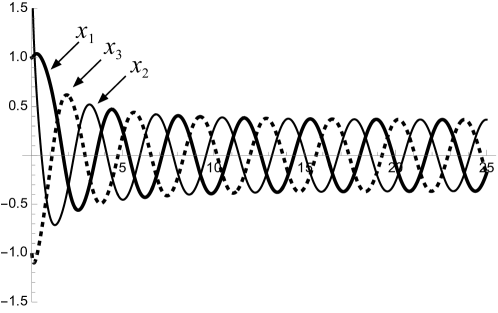
Figure 3: Periodic state created by Hopf bifurcation in a $\mathbb{Z}_{3}$-symmetric ring. Solid thick = $x_{1}$, solid thin = $x_{2}$, dashed = $x_{3}$. Parameters $a_{0}=-0.9,a_{1}=-2$ (just after bifurcation).

Figure 3 shows a simulation for parameter values $a_{0}=-0.9,a_{1}=-2$. The oscillations have a clear phase pattern of the form

$$x(t)=(u(t),u(t-2T/3),u(t-T/3))$$

where $T$ is the period and $u(t)$ is the common waveform at each node. The time-reversal of this ODE yields a rotating wave in the opposite direction:

$$x(t)=(u(t),u(t-T/3),u(t-2T/3))$$

In Section 4 we discuss how the rotating wave structure is generated by the $\mathbb{Z}_{3}$ symmetry, and is related to the form of the eigenvectors $u_{1}$ and $u_{2}$.

3 Equivariant and Network Dynamics

The dynamics and bifurcations of ring networks can be studied within two different frameworks: equivariant dynamics [42] and network dynamics [39]. The first focuses on symmetry properties; the second on the topology (and type) of connections. Neither alone captures the behaviour of ring networks. In particular, generic dynamics for a network with symmetry group $\Gamma$ can differ from generic $\Gamma$-equivariant dynamics [39]. Symmetry and topology can interact to create new generic phenomena. In practice, symmetric networks are studied using a combination of equivariant and network dynamics, while bearing in mind the potential for unusual behaviour.

However, equivariant dynamics suffices for the purposes of this paper, with one additional constraint: the variables that appear in model ODEs must respect the network topology; see Section 3.2. We therefore refer to [43, 39, 73] for information on general network dynamics, and use the equivariant approach. Symmetric ring networks are quite well behaved in this regard, as we summarise briefly in Section 7.

Hopf bifurcation for systems with dihedral group symmetry $\mathbb{D}_{n}$ is analysed in [37]; see also [38, 42]. Hopf bifurcation for systems with cyclic group symmetry $\mathbb{Z}_{n}$ iis mentioned briefly in [42, Chapter XVII Section 8(b)]. We supply further detail and prove some new results.

3.1 Equivariant Dynamics

Equivariant dynamics examines how the symmetries of a differential equation affect the behavior of its solutions, especially their symmetries. To describe the main results we require some basic concepts.

For simplicity, assume that the state space of the system is $X=\mathbb{R}^{n}$ and consider an ODE

$$\dot{x}=f(x)\qquad x\in X$$ (5)

where $f:X\rightarrow X$ is a smooth map (vector field). Symmetries enter the picture when a group of linear transformations $\Gamma$ acts on $X$. We require all elements of $\Gamma$ to map solutions of the ODE to solutions. By [38, Section 1.2] this is equivalent to $f$ being $\Gamma$-equivariant; that is:

$$f(\gamma x)=\gamma f(x)$$ (6)

for all $\gamma\in\Gamma,x\in X$. We call (5) a $\Gamma$-equivariant ODE.

Condition E:equivar captures the structure of ODEs that arise when modeling a symmetric real-world system. It states that the vector field inherits the symmetries, in the sense that symmetrically related points in state space have symmetrically related vectors.

For bifurcation theory, we consider a parametrised family of ODEs

$$\dot{x}=f(x,\lambda)\qquad x\in X$$ (7)

The equivariance condition is then:

$$f(\gamma x,\lambda)=\gamma f(x,\lambda)$$ (8)

for all $\gamma\in\Gamma,x\in X$. We call (7) a $\Gamma$-equivariant family of ODEs.

3.2 Admissible ODEs in Network Dynamics

A network of coupled ODEs is represented by a directed graph (or digraph) in which: (a) Each node corresponds to a component ODE. Nodes are classified into distinct node-types.

(b) Each arrow (directed edge) indicates coupling: the node at the head of the arrow receives an input from the node at the tail end. Arrows are classified into distinct arrow-types.

We call such a system of ODEs a network system. The directed graph is the network diagram. The head of node $c$ is denoted by $\mathcal{H}(c)$ and the tail by $\mathcal{T}(c)$.

For each node $c$ choose a node space $P_{c}=\mathbb{R}^{n_{c}}$ and corresponding node coordinates $x_{c}$ on $P_{c}$. These coordinates are multidimensional if $\dim P_{c}>1$. Nodes of the same state-type have the same coordinate system and their dynamics can meaningfully be compared. The total state space is $P=\oplus_{c}P_{c}$.

A map $f=(f_{1},\ldots,f_{n})$ from $P$ to itself can be written in components as

$$f_{c}:P\rightarrow P_{c}\qquad 1\leq c\leq n$$

For admissibility we impose extra conditions on the $f_{c}$ that reflect network architecture. See [43, 39, 73] for details; here we summarise the main idea.

Definition 3.1.

A map $f:P\rightarrow P$ is ${\mathcal{G}}$-admissible if:

(1) Domain Condition: For every node $c$, the component $f_{c}$ depends only on the node variable $x_{c}$ and the input variables $x_{i}$ where $i$ runs through the tail nodes of arrows with head $c$; see equation (10) below.

(2) Symmetry Condition: If $c$ is a node, $f_{c}$ is invariant under all permutations of tail node coordinates for input arrows of the same type.

(3) Pullback Condition: If nodes $c$ and $d$ have the same node-type, and the same number of input arrows of any given type, then the components $f_{c},f_{d}$ are identical as functions. The variables to which they are applied correspond under some (hence any, by condition (2)) bijection that preserves the arrow-types.

Conditions (2) and (3) can be combined into a single pullback condition applying to any pair $c,d$ of nodes, but it is convenient to separate them.

Each admissible map $f$ determines an admissible ODE

$$\dot{x}=f(x)$$ (9)

In node coordinates this takes the form

$$\dot{x}_{c}=f_{c}(x_{c},x_{i_{1}},\ldots,x_{i_{m}})$$ (10)

for all nodes $c$, where $i_{1},\ldots,i_{m}$ are the tails of the arrows with head $c$; that is, the input variables to node $c$.

Equation (3) is an example of an admissible ODE for a 3-node unidirectional NN coupled ring in which all nodes have the same node-type and all arrows have the same arrow-type (which is equivalent to $\mathbb{Z}_{3}$ symmetry in this case). In particular, the only variables appearing in the component for $\dot{x}_{c}$ are $x_{c}$ itself and $x_{c-1}$, the variable corresponding to the tail of the unique input arrow.

If $f$ also depends on a (possibly multidimensional) parameter $\lambda$, and is admissible as a function of $x$ for any fixed $\lambda$, we have an admissible family of maps $f(x,\lambda)$ and ODEs $\dot{x}=f(x,\lambda)$. Such families arise in bifurcation theory.

If the network has symmetry group $\Gamma$, every admissible map is $\Gamma$-equivariant. However, the converse is false in general; see [39, Section 16.5] and Section 7.

3.3 Local Bifurcation in Equivariant Dynamics

Isotropy Subgroups and Fixed-Point Subspaces

Recall that if $x(t)$ is a solution of a $\Gamma$-equivariant ODE, then so is $\gamma x(t)$ for all $\gamma\in\Gamma$. Suppose that an equilibrium $x_{0}$ is unique. Then $\gamma x_{0}$ is also an equilibrium, so by uniquenesss, $\gamma x_{0}=x_{0}$ for all $\gamma\in\Gamma$. Thus the solution is symmetric under $\Gamma$. However, when uniqueness fails—which is common in nonlinear dynamics—equilibria of a $\Gamma$-equivariant ODE need not be symmetric under the whole of $\Gamma$. This phenomenon, called (spontaneous) symmetry-breaking, is a general mechanism for pattern formation.

Symmetry of a Solution

To formalise ‘symmetry of a solution’ we introduce a key concept:

Definition 3.2.

If $x\in X$, the isotropy subgroup of $x$ is

$$\Sigma_{x}=\{\sigma\in\Gamma:\sigma x=x\}$$

This group consists of all $\sigma$ that fix $x$.

Similarly the isotropy subgroup of a solution $x(t)$ is

$$\Sigma_{x(t)}=\{\sigma\in\Gamma:\sigma x(t)=x(t)\ \forall t\}$$

Example 3.3.

We revisit Example 2.2 with $\Gamma=\mathbb{Z}_{3}\times\mathbb{Z}_{2}$. Solutions on the trivial branch $x=0$ have isotropy subgroup $\Gamma$. Solutions on the bifurcating branch of periodic oscillations have isotropy subgroup $\mathbb{Z}_{2}$.

There is a ‘dual’ notion. If $\Sigma\subseteq\Gamma$ is a subgroup of $\Gamma$, its fixed-point subspace is

$$\mbox{{\rm Fix}}(\Sigma)=\{x\in X:\sigma x=x\quad\forall\sigma\in\Sigma\}$$

Clearly $\mbox{{\rm Fix}}(\Sigma)$ comprises all points $x\in X$ whose isotropy subgroup contains $\Sigma$. Fixed-point spaces provide a natural class of subspaces that are invariant for any $\Gamma$-equivariant map $f$:

Proposition 3.4.

Let $f:X\rightarrow X$ be a $\Gamma$-equivariant map, and let $\Sigma$ be any subgroup of $\Gamma$. Then $\mbox{{\rm Fix}}(\Sigma)$ is an invariant subspace for $f$, and hence for the dynamics of (5).

The proof is so simple that we give it here:

Proof.

If $x\in\mbox{{\rm Fix}}(\Sigma)$ and $\sigma\in\Sigma$, then

$$\sigma f(x)=f(\sigma x)=f(x)$$

so $f(x)\in\mbox{{\rm Fix}}(\Sigma)$. ∎

Corollary 3.5.

The isotropy subgroup of a solution $x(t)$ is the same as that of any point $x(t_{0})$ on it.

Proof.

If $x(t_{0})\in Y$ where $Y$ is an invariant subspace, then $x(t)\in Y$ for all $t$. ∎

We can interpret $\mbox{{\rm Fix}}(\Sigma)$ as the space of all states that have symmetry (at least) $\Sigma$. Then the restriction

$$f|_{\mbox{{\rm Fix}}(\Sigma)}$$

determines the dynamics of all such states. In particular, we can find states with a given isotropy subgroup $\Sigma$ by considering the (generally) lower-dimensional system determined by $f|_{\mbox{{\rm Fix}}(\Sigma)}$.

If $x\in X$ and $\gamma\in\Gamma$, the isotropy subgroup of $\gamma x$ is conjugate to that of $x$:

$$\Sigma_{\gamma x}=\gamma\Sigma_{x}\gamma^{-1}$$

Therefore isotropy subgroups occur in conjugacy classes, which correspond to group orbits of solutions. For many purposes we can consider isotropy subgroups only up to conjugacy. The conjugacy classes of isotropy subgroups are ordered by inclusion (up to conjugacy). The resulting partially ordered set is called the lattice of isotropy subgroups or isotropy lattice [42], although technically it need not be a lattice. (If we do not pass to conjugacy classes, it is a lattice, and it is often a lattice when we do.)

3.4 Review of Representation Theory

The structure of equivariant ODEs is tightly constrained by the representation of the symmetry group on the state space. In this paper all symmetry groups are compact Lie groups (especially finite groups) $\Gamma$ acting linearly on $X=\mathbb{R}^{k}$ for some finite $k$. That is, if $x\in X,\gamma\in\Gamma$ there are linear maps $\rho_{\gamma}:X\to X$ such that

$$\rho_{1}=I_{k}\qquad\rho_{\gamma\delta}(x)=\rho_{\gamma}(\rho_{\delta}(x))$$

for all $x\in X,\gamma,\delta\in\Gamma$, where $I_{k}$ is the identity matrix and $1$ is the identity element of $\Gamma$. We write

$$\gamma x=\rho_{\gamma}(x)$$

and use the term ‘representation’ both for the action $\rho$ and for the representation space $X$. If $Y\subseteq X$ is $\Gamma$-invariant, so that $\gamma y\in Y$ whenever $y\in Y$, the restriction $\rho|_{Y}$ of the action of $\Gamma$ to $Y$ is also a representation, called a subrepresentation or component of $X$. A representation $X$ is irreducible if the only $\Gamma$-invariant subspaces are $0$ and $X$. In the compact case, any representation $X$ is completely reducible:

$$X=X_{1}\oplus\cdots\oplus X_{m}$$

where the $X_{i}$ are irreducible.

If $X$ is irreducible, the space $\mathcal{D}$ of linear $\Gamma$-equivariant maps $L:X\to X$ is an associative algebra over $\mathbb{R}$. By Schur’s Lemma it is a division algebra over $\mathbb{R}$, so $\mathcal{D}$ is isomorphic to precisely one of $\mathbb{R},\mathbb{C}$, and $\mathbb{H}$, where $\mathbb{H}$ is the quaternions. We say that $X$ is absolutely irreducible if $\mathcal{D}\cong\mathbb{R}$, and non-absolutely irreducible if $\mathcal{D}\cong\mathbb{C}$ or $\mathbb{H}$.

A component $W$ is $\Gamma$-simple if and only if either

(a) $W\cong V\oplus V$ where $V$ is absolutely irreducible, or

(b) $W$ is non-absolutely irreducible.

For each irreducible component $Y\subseteq X$, the corresponding isotypic component $W_{Y}$ is defined to be the sum of all irreducible components isomorphic to $Y$. It can be written as

$$W_{Y}=Y_{1}\oplus\cdots\oplus Y_{c}$$

where every $Y_{i}$ is isomorphic to $Y$. Each isotypic component is invariant under all linear equivariant maps $L:X\to X$.

Representation-Theoretic Conditions for Equivariant Hopf Bifurcation

Consider a $\Gamma$-equivariant family of ODEs

$$\dot{x}=f(x,\lambda)\qquad(x\in X=\mathbb{R}^{k},\lambda\in\Lambda=\mathbb{R})$$

Suppose that a Hopf bifurcation from a branch of fully symmetric equilibria occurs at $(x_{0},\lambda_{0})$. Translating coordinates we may assume $x_{0}=0,\lambda_{0}=0$, and we do this from now on. Then ${\mathrm{D}}f|_{(0,0)}$ has eigenvalues $\pm\omega\mathrm{i}$ for $\omega\neq 0$. This can happen only if $X$ contains a $\Gamma$-simple component. The critical eigenspace $E_{\pm\mathrm{i}\omega}$ is $\Gamma$-invariant, and generically it is $\Gamma$-simple. Thus ‘$\Gamma$-simple component’ is the equivariant analogue of ‘simple eigenvalue’ in ordinary dynamical systems. Moreover, there exists an equivariant coordinate change on $E_{\pm\mathrm{i}\omega}$ such that, in the new coordinates,

$${\mathrm{D}}f|_{(0,0)}=J=\left[\begin{array}[]{ccccccccccccccccccccccccr}0&-\omega I_{m}\\ \omega I_{m}&0\end{array}\right]$$

where $\dim_{\mathbb{R}}E_{\pm\mathrm{i}\omega}=2m$. The matrix $J$ commutes with the symmetry group and defines an action of the circle group ${\bf S}^{1}=\mathbb{R}/2\pi\mathbb{Z}$ on $E_{\pm\mathrm{i}\omega}$ by

$$\theta x=\exp(\theta J/|\omega|)x$$

This gives $E_{\pm\mathrm{i}\omega}$ the structure of a complex vector space, in which

$$(r{\mathrm{e}}^{\mathrm{i}\theta})x=r\,\theta x$$

This is not the usual complexification $\mathbb{C}\otimes_{\mathbb{R}}E_{\pm\mathrm{i}\omega}$; in particular the dimension of the latter over $\mathbb{R}$ is twice that of $E_{\pm\mathrm{i}\omega}$.

The group $\Gamma\times{\bf S}^{1}$ now acts on $E_{\pm\mathrm{i}\omega}$ by

$$(\gamma,\theta)x=\theta\,\gamma x=\exp(\theta J/|\omega|)\gamma x$$

This extra circle action induces phase patterns on bifurcating branches of periodic solutions.

Symmetry-Breaking

Spontaneous symmetry-breaking in a $\Gamma$-equivariant ODE occurs when the isotropy subgroup of a solution $x(t)$ is smaller than $\Gamma$.

The basic general existence theorem for bifurcating symmetry-breaking equilibria is the Equivariant Branching Lemma of Cicogna [16] and Vanderbauwhede [77]. See [42, 38]. Two kinds of existence theorem for periodic solutions in equivariant systems have been developed over the past 30 years. Both are aimed at understanding the kinds of spatiotemporal symmetries of periodic states that can be expected in such systems. One is the Equivariant Hopf Theorem [36, 38, 42]; the other is the $H/K$ Theorem [13]. Both have analogues for network dynamics [39]. In this paper only the Equivariant Hopf Theorem is required. It is an analogue of the Equivariant Branching Lemma and is proved by Liapunov-Schmidt reduction from an operator equation on loop space [36, 42].

At a non-zero imaginary critical eigenvalue, the critical eigenspace $E$ supports an action not just of $\Gamma$, but of $\Gamma\times{\bf S}^{1}$. This action is preserved by Liapunov-Schmidt reduction [42, Chapter XVI Section 3]. The ${\bf S}^{1}$-action on the critical eigenspace is related to, but different from, the phase shift action; it is determined by the exponential of the Jacobian $J|_{E}$ on $E$. Specifically, if the imaginary eigenvalues are $\pm\mathrm{i}\omega$ with $\omega\neq 0$ then $\theta\in{\bf S}^{1}$ acts on $E$ like the matrix $\exp(\frac{\theta}{|\omega|}J|_{E})$. The ${\bf S}^{1}$-action on solutions is by phase shift, induced via the Liapunov-Schmidt reduction procedure.

The Equivariant Hopf Theorem is analogous to the Equivariant Branching Lemma, but the symmetry group $\Gamma$ is replaced by $\Gamma\times{\bf S}^{1}$.

Definition 3.6.

A subgroup $\Sigma\subset\Gamma\times{\bf S}^{1}$ is $\mathbb{C}$-axial if $\Sigma$ is an isotropy subgroup for the action of $\Gamma\times{\bf S}^{1}$ on $E$ and $\dim_{\mathbb{R}}\mbox{{\rm Fix}}(\Sigma)=2$.

Theorem 3.7 (Equivariant Hopf Theorem).

If the Jacobian has non-real purely imaginary eigenvalues $\pm\mathrm{i}\omega$, then generically for any $\mathbb{C}$-axial subgroup $\Sigma\subseteq\Gamma\times{\bf S}^{1}$ acting on the critical eigenspace, there exists a branch of periodic solutions with spatiotemporal symmetry group $\Sigma$. The period tends to $T=\frac{2\pi}{|\omega|}$ at the bifurcation point. On solutions, ${\bf S}^{1}$ acts by phase shifts.

Proof.

See [36, Theorem 5.1], [38, Theorem 4.9], or [42, Chapter XVI Theorem 4.1]. ∎

The isotropy subgroup in $\Gamma\times{\bf S}^{1}$ of a periodic solution is a twisted subgroup

$$H^{\phi}=\{(h,\phi(h):h\in H\}$$ (11)

where $H$ is a subgroup of $\Gamma$ and $\phi:\Gamma\to{\bf S}^{1}$ is a homomorphism. The kernel $K=\ker\phi\subseteq\Gamma$ is the group of spatial symmetries, and $H$ is the group of spatiotemporal symmetries. The quotient $H/K$ determines the phase shifts of the corresponding phase pattern. Since $H/K$ embeds in ${\bf S}^{1}$, either $H/K\cong{\bf S}^{1}$ or $H/K\cong\mathbb{Z}_{k}$ for some $k$. Possible pairs $(H,K)$ are classified in [13]; see also [33]. Not all can be obtained via Hopf bifurcation from a fully symmetric equilibrium [28].

Equivariant Hopf bifurcations have been studied when the group $\Gamma$ is:

$\mathbb{Z}_{n}$ [42, Chapter XVII Section 8]

$\mathbb{D}_{n}$ [37],[42, Chapter XVIII Sections 1–4]

$\mathbb{S}_{n}$ [72]

$\mathbb{O}(2)$ [42, Chapter XVII]

$\mathbb{S}\mathbb{O}(2)$ [42, Chapter XVII Section 8]

$\mathbb{O}(3)$ [42, Chapter XVIII Section 5]

$\mathbb{S}\mathbb{O}(n)$ [42, Chapter XVII Section 5]

$\mathbb{S}_{n}\times\mathbb{O}(2)$ [72]

Symmetry group of hexagonal lattice [42, Chapter XVIII Section 6], [70]

Symmetry groups of planar lattices [22, 42]

Symmetry group of cubic lattice $\mathbb{Z}^{3}$ [20]

Network Analogues

There are natural analogues of the Equivariant Hopf Theorem and the $H/K$ Theorem for networks [39]. The Network Hopf Theorem has a rigorous proof; that of the Network $H/K$ Theorem rests on some ‘Rigidity Conjectures’, as yet proved only in special cases or under stronger hypotheses. See [39, Chapters 15, 17]. We omit details.

Time-Reversal

The next Proposition, about reversing time in an ODE and a given solution, is trivial but important.

Proposition 3.8.

Consider a periodic state with period normalised to $2\pi$. If a phase pattern with phase shifts $\theta_{i}$ occurs for an admissible ODE $\dot{x}=f(x)$, then the reverse pattern with phase shifts $2\pi-\theta_{i}$ occurs for the admissible ODE $\dot{x}=-f(x)$.

Proof.

If $f$ is equivariant or admissible then so is $-f$. Now assume that $x(t)$ is a periodic solution of $\dot{x}=f(x)$, and define $s=-t$ and $y(s)=x(-s)=x(t)$. Then

$$\frac{\mathrm{d}}{\mathrm{d}s}y(s)=-\frac{\mathrm{d}}{\mathrm{d}t}y(s)=-\frac{\mathrm{d}}{\mathrm{d}t}x(t)=-f(x(t))=-f(y(s))$$

Therefore changing $f$ to $-f$ reverses time, and a solution $x(t)$ for $f$ becomes a solution $y(s)$ for $-f$. A phase pattern $(\theta_{i})$ for $x$ therefore becomes $(-\theta_{i})$ for $y$. Normalising to $\theta_{i}\in[0,2\pi)$ this becomes $(2\pi-\theta_{i})$. ∎

Proposition 3.9.

If the admissible ODE $\dot{x}=f(x,\lambda)$ has a Hopf bifurcation at $(x_{0},\lambda_{0})$, then the time-reversal $\dot{x}=-f(x,\lambda)$ has a Hopf bifurcation at $(-x_{0},\lambda_{0})$.

Proof.

The Jacobians satisfy

$${\mathrm{D}}(-f)|_{(-x_{0},\lambda_{0})}=-{\mathrm{D}}f|_{(x_{0},\lambda_{0})}$$

The eigenvalues of ${\mathrm{D}}(-f)|_{(-x_{0},\lambda_{0})}$ are minus those of ${\mathrm{D}}f|_{(x_{0},\lambda_{0})}$. So ${\mathrm{D}}(-f)|_{(-x_{0},\lambda_{0})}$ has eigenvalues $\mp\mathrm{i}\omega$ if and only if ${\mathrm{D}}f|_{(x_{0},\lambda_{0})}$ has eigenvalues $\pm\mathrm{i}\omega$.

Moreover, the non-resonance and eigenvalue crossing conditions for ${\mathrm{D}}(-f)|_{(-x_{0},\lambda_{0})}$ are trivially equivalent to those for ${\mathrm{D}}f|_{(x_{0},\lambda_{0})}$. ∎

4 Symmetric Unidirectional Rings

Consider a symmetric unidirectional $n$-node ring ${\mathcal{U}}_{n}$ with NN coupling.

4.1 1-Dimensional Node Spaces

Initially we assume that the node spaces are $1$-dimensional, that is, $\mathbb{R}$. Figure 2 (left) shows the case $n=5$. This network has $\mathbb{Z}_{n}$ symmetry, generated by an element $\alpha$. If we number the nodes as ${\mathcal{C}}=\{0,1,\ldots,n-1\}$ then the symmetry group acts by $\alpha^{k}(c)=c+k\pmod{n}$.

Admissible ODEs have the form

$$\dot{x}_{c}=f(x_{c},x_{c+1})\qquad c\in{\mathcal{C}}$$ (12)

where again we take addition modulo $n$. The linear admissible maps are all linear combinations $L=a_{0}I+a_{1}A$ of the two matrices:

$$I=\left[\begin{array}[]{ccccccccccccccccccccccccr}1&0&0&\cdots&0\\ 0&1&0&\cdots&0\\ 0&0&1&\cdots&0\\ \vdots&\vdots&\vdots&\ddots&\vdots\\ 0&0&0&\cdots&1\end{array}\right]\qquad A=\left[\begin{array}[]{ccccccccccccccccccccccccr}0&1&0&\cdots&0\\ 0&0&1&\cdots&0\\ 0&0&0&\ddots&0\\ \vdots&\vdots&\vdots&\ddots&\vdots\\ 1&0&0&\cdots&0\end{array}\right]$$ (13)

where the matrix $A$ is the adjacency matrix for NN coupling.

By symmetry, the eigenspaces of $L$ can be deduced from the natural permutation representation of $\mathbb{Z}_{n}$ on $\mathbb{R}^{n}$. The isotypic components are the spaces $V_{k}=\Re(\mathbb{C}\{v_{k},v_{n-k}\})$ where $\Re$ is the real part and

$$v_{k}=[1,\zeta^{k},\zeta^{2k},\ldots,\zeta^{n-1}]^{\mathrm{T}}$$

Then $L$ acts on $V_{k}$ by

$$v_{k}\mapsto(a_{0}+\zeta^{k}a_{1})v_{k}$$

so the eigenvalues of $L$ are

$$\mu_{k}=a_{0}+\zeta^{k}a_{1}$$

and each eigenvalue is simple provided that $a_{1}\neq 0$. (If $a_{1}=0$ no Hopf bifurcation occurs since all eigenvalues are real; this case is dynamically uninteresting since the nodes are decoupled.)

For Hopf bifurcation there are two cases: $n$ odd and $n$ even.

Case 1: $n$ odd.

When $n=2m+1$ there is one real root of unity $\zeta^{0}=1$, and the others occur as $m$ complex conjugate pairs $\zeta^{r}$ and $\zeta^{n-r}=\bar{\zeta}^{r}$ for $1\leq r\leq m$. The corresponding real eigenspaces have dimension 1 and 2, respectively. Hopf bifurcation can occur only for a 2-dimensional critical eigenspace, so $\zeta^{0}$ does not occur and $1\leq r\leq m$. The other real eigenspaces afford irreducible representations of $\mathbb{Z}_{n}$, and these are non-absolutely irreducible, of complex type.

A necessary (though not sufficient) condition for a Hopf branch from the trivial solution to be stable is that it is spawned by the first bifurcation. That is, when the corresponding eigenvalues becomes critical (as the bifurcation parameter $\lambda$ increases), all other eigenvalues have negative real part.

When node spaces are 1-dimensional and the ring topology is NN, there are strong constraints on the possible eigenvalues for the first bifurcation to be a Hopf bifurcation.

Theorem 4.1.

Let ${\mathcal{G}}$ be a $\mathbb{Z}_{n}$-symmetric ring with unidirectional NN coupling and 1-dimensional node spaces. Then the first local bifurcation is Hopf if and only if $n=2N+1$ is odd. In that case the critical eigenvalues are the $\rho_{k}$ for $k=N,N+1$.

Proof.

When $a_{1}>0$ the real parts of the eigenvalues are ordered in the same manner as the real parts of $\zeta^{r}$, that is,

$$\cos\frac{2\pi N}{2N+1}<\cos\frac{2\pi(N-1)}{2N+1}<\cdots<\cos\frac{2\pi}{2N+1}<1$$

so the first bifurcation is not Hopf.

When $a_{1}<0$ the order is the reverse of this, so the first bifurcation occurs for $\zeta^{N}$ with real part $\cos\frac{2\pi N}{2N+1}$. It is a Hopf bifurcation.

Case 2: $n$ even.

When $n=2N$ there are two real roots of unity: $\zeta^{0}=1$ and $\zeta^{N}=-1$. The others occur as $N-1$ complex conjugate pairs $\zeta^{r}$ and $\zeta^{n-r}=\bar{\zeta}^{r}$ for $1\leq r\leq N-1$. The corresponding real eigenspaces have dimension 1 and 2, respectively. Hopf bifurcation can occur only for a 2-dimensional critical eigenspace, so $\zeta^{0}$ and $\zeta^{N}$ do not occur and $1\leq r\leq N-1$. The other real eigenspaces afford irreducible representations of $\mathbb{Z}_{n}$, and these are non-absolutely irreducible of complex type.

Again when $a_{1}>0$ the real parts of the eigenvalues are ordered in the same manner as the real parts of $\zeta^{r}$, which are now

$$-1<\cos\frac{2\pi(N-1)}{2N}<\cos\frac{2\pi(N-2)}{2N}<\cdots<\cos\frac{2\pi}{2N}<1$$

When $a_{1}<0$ the ordering is the reverse. The first bifurcation occurs for the eigenvalue $a_{0}+a_{1}\zeta^{r}$ where $r=0,N$ respectively. That is, for $a_{0}\pm a_{1}$. Since this is real, the first bifurcation cannot be Hopf. ∎

Example 4.2.

Consider the following $\mathbb{Z}_{5}$-equivariant ODE in variables $x=(x_{0},x_{1},x_{2},x_{3},x_{4})$:

$$\begin{array}[]{rcl}\dot{x}_{0}&=&\lambda x_{0}-x_{0}^{3}+ax_{4}\\ \dot{x}_{1}&=&\lambda x_{1}-x_{1}^{3}+ax_{0}\\ \dot{x}_{2}&=&\lambda x_{2}-x_{2}^{3}+ax_{1}\\ \dot{x}_{3}&=&\lambda x_{3}-x_{3}^{3}+ax_{2}\\ \dot{x}_{4}&=&\lambda x_{4}-x_{4}^{3}+ax_{3}\end{array}$$ (14)

where $\lambda$ acts as a bifurcation parameter and $a$ is a coupling strength. (Again there is an extra symmetry $x\mapsto-x$, which we can remove with a small quadratic term. See Section 5.1.) There is an equilibrium at $[0,0,0]^{\mathrm{T}}$ for all $\lambda$.

Figure 4 shows a simulation of a rotating wave for parameter values $\lambda=-1.1,a=-2$. We omit the eigenvalue analysis, which follows from Theorem 4.1.

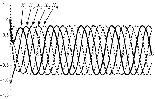
Figure 4: Hopf bifurcation in a $\mathbb{Z}_{5}$ ring for the ODE (14). Horizontal coordinate: $\lambda$. Vertical coordinates: $x_{i}$ for $0\leq i\leq 4$. Thick solid = node 1, thick dash = node 2, thin solid = node 3, thin dash = node 4, thick dot-dash = node 5. Parameters $\lambda=-1.1,a=-2$.

In this simulation the succession of nodes for phase shifts of $T/5$ are $1\ 3\ 5\ 2\ 4$. Equivalently, the phase shifts for nodes in cyclic order $1\ 2\ 3\ 4\ 5$ are $0,2T/5,4T/5,T/5,3T/5$, corresponding to the critical eigenvalue pair $\mu_{2},\mu_{3}$ (where $\mu_{3}=\bar{\mu}_{2}$). This is in accordance with the ‘first bifurcation’ condition of Theorem 4.1. Time reversal leads to the reverse order $0,3T/5,T/5,4T/5,2T/5$.

There is no oscillatory fully synchronous state, since nodes are 1-dimensional. Phase shifts $0,T/5,2T/5,3T/5,4T/5$ and the reverse can occur, but not stably.

Again there is a further symmetry $x\mapsto-x$: see Section 5.1.

Longer range connections or higher-dimensional node spaces allow other oscillatory modes to be the first bifurcation. See Sections 5.2 and 6.

5 Hopf Bifurcation in the NN Unidirectional Ring

When the symmetry group $\Gamma$ is abelian, and in particular when it is cyclic, generic Hopf bifurcation in a $\Gamma$-equivariant system occurs at simple eigenvalues, because irreducibles are 1-dimensional over $\mathbb{C}$, hence either 1-dimensional over $\mathbb{R}$ or 2-dimensional over $\mathbb{R}$ with eigenvalues $\pm\mathrm{i}\omega$ with $\omega\neq 0$. Thus the classical Hopf Bifurcation Theorem applies. At first sight this might seem to make the Equivariant Hopf Theorem superfluous, but it is not. It provides extra information on the spatiotemporal symmetries of the bifurcating branch of periodic solutions.

To see how this occurs, we apply the Equivariant Hopf Theorem to the $\mathbb{Z}_{n}$-symmetric NN-coupled unidirectional ring. The symmetry group is $\Gamma=\mathbb{Z}_{n}$ acting on $\mathbb{R}^{n}$ by permuting coordinates according to the $n$-cycle $\alpha$, and $\mathbb{Z}_{n}=\langle\alpha\rangle$. Extend the base field to $\mathbb{C}$ so that $\Gamma$ acts on $\mathbb{C}^{n}$. The $\mathbb{C}$-irreducible subspaces are the eigenspaces $W_{k}=\mathbb{C}\{v_{k}\}$. The $\mathbb{R}$-irreducible subspaces are the real eigenspaces, which are the real parts $V_{k}$ of $\mathbb{C}\{v_{k},v_{n-k}\}=w_{k}+W_{n-k}$. The Jacobian ${\mathrm{D}}f$ is $a_{0}I+a_{1}A$ for $a_{0},a_{1}\in\mathbb{R}$. The eigenvalues on $V_{k}$ are $a_{0}+a_{1}\zeta^{k}$ and $a_{0}+a_{1}\zeta^{n-k}$. That is,

$$a_{0}+a_{1}(\cos\frac{2k\pi}{n}\pm\mathrm{i}\sin\frac{2k\pi}{n})$$

For Hopf bifurcation,

$$0=a_{0}+a_{1}\cos\frac{2k\pi}{n}$$

and the eigenvalues are $\pm\mathrm{i}\omega$ where

$$\omega=|a_{1}\sin\frac{2k\pi}{n}|=|a_{1}|$$

since $0\leq k\leq n/2$. Here we take the absolute value because, when defining the ${\bf S}^{1}$-action, we take the value of $\omega$ to be positive. (This is important later when we consider the direction in which the wave rotates.)

Working on $W_{k}$, the cycle $\alpha$ acts as the matrix $A$, and on $W_{k}$ this restricts to

$$A_{k}=\left[\begin{array}[]{ccccccccccccccccccccccccr}\zeta^{k}&0\\ 0&\zeta^{-k}\end{array}\right]$$

The ${\bf S}^{1}$-action induced from Liapunov-Schmidt reduction is given by $\theta$ acting as

$$M_{\theta}=\exp(A\theta/\omega)=\exp\left[\begin{array}[]{ccccccccccccccccccccccccr}\pm\mathrm{i}\theta&0\\ 0&\mp\mathrm{i}\theta\end{array}\right]=\left[\begin{array}[]{ccccccccccccccccccccccccr}{\mathrm{e}}^{\pm\mathrm{i}\theta}&0\\ 0&{\mathrm{e}}^{\mp\mathrm{i}\theta}\end{array}\right]$$

where the sign $\pm$ is that of $b$ and $\mp$ is the opposite sign. Therefore $(\alpha,\theta)$ acts as

$$AM_{\theta}=\left[\begin{array}[]{ccccccccccccccccccccccccr}{\mathrm{e}}^{\mathrm{i}(\frac{2k\pi}{n}\pm\theta)}&0\\ 0&{\mathrm{e}}^{-\mathrm{i}(\frac{2k\pi}{n}\mp\theta)}\end{array}\right]$$

This gives a 2-dimensional fixed-point space (namely the whole of $V_{k}$) if and only if

$$\theta=\mp\frac{2k\pi}{n}$$

When $k\neq 0$ this is the rotating wave condition; when $k=0$ it gives a fully synchronous standing wave. In either case the solution is fixed by $(\alpha,\mp\frac{2k\pi}{n})$.

Moreover, we can read off the direction of rotation. It is determined by the sign of $\sin\frac{2k\pi}{n}$.

Theorem 5.1.

Let ${\mathcal{G}}$ be a unidirectional ring of $1$-dimensional nodes with $\mathbb{Z}_{n}$ symmetry, obeying the ODE (12). Suppose the critical eigenvalues are those on $V_{k}$, where $k\neq 0$ and $k\neq n/2$ for $n$ even. Then generically there is a bifurcating branch of periodic solutions of the form

$$x_{j}(t)=\phi(t\pm jT/k)$$ (15)

for a $T$-periodic function $\phi$. (Here we take the same sign $+$ or $-$ throughout.)

The period $T$ converges to $2\pi/|\omega|$ at the bifurcation point. The sign in (15) is that of $a_{1}$.

Proof.

The spaces $V_{k}$ are the irreducible subspaces for the $\mathbb{Z}_{n}$-action. When $k\neq 0$ and $k\neq n/2$ for $n$ even, these are non-absolutely irreducible and of complex type. Over $\mathbb{R}$ they have dimension 2.

The complexified actions of $\alpha\in\mathbb{Z}_{n}$ and $\theta\in{\bf S}^{1}$ are by the matrices

$$\alpha=\left[\begin{array}[]{ccccccccccccccccccccccccr}{\mathrm{e}}^{2\pi\mathrm{i}/n}&0\\ 0&{\mathrm{e}}^{-2\pi\mathrm{i}/n}\end{array}\right]\qquad\theta=\left[\begin{array}[]{ccccccccccccccccccccccccr}{\mathrm{e}}^{\mathrm{i}\theta}&0\\ 0&{\mathrm{e}}^{-\mathrm{i}\theta}\end{array}\right]$$

Therefore $(\alpha,-2\pi/n)$ acts as the identity. Taking the real part, the group

$$\tilde{\mathbb{Z}}_{3}=\langle(\alpha,-2\pi/n)\rangle$$

is $\mathbb{C}$-axial. By the equivariant Hopf Theorem, there is a bifurcating branch of periodic states with spatiotemporal symmetry group $\tilde{\mathbb{Z}}_{n}$. On $V_{k}$ this gives rise to solutions of the form (15). (The $\pm$ sign in (15) is explained in Section 5.4.) ∎

5.1 Examples 2.2 and 4.2 Revisited

The ODE (3) is also equivariant under $x\mapsto-x$, so the symmetry group is actually $\mathbb{Z}_{3}\times\mathbb{Z}_{2}\cong\mathbb{Z}_{6}$. In the Equivariant Hopf Theorem, this extra symmetry identifies with a half-period phase shift, since both induce minus the identity. We do not get extra solution branches, but now all solutions are fixed by the ‘glide reflection’ symmetry $x(t)\mapsto-x(t-T/2)$ of the time series. To destroy this symmetry we can add a small quadratic term. The rotating wave state persists.

Similarly, Example 4.2 is also equivariant under $x\mapsto-x$. So the symmetry group is actually $\mathbb{Z}_{5}\times\mathbb{Z}_{2}\cong\mathbb{Z}_{10}$. Again, solutions are fixed by $x(t)\mapsto-x(t-T/2)$.

5.2 Longer-Range Coupling

We can consider rings with the same cyclic group symmetry but longer-range coupling, and now the first bifurcation is less tightly constrained. The results in this section appear to be new.

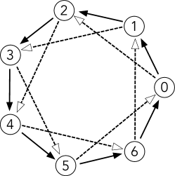
Figure 5: A $7$-node ring with NN (solid arrows) and NNN (dashed arrows) coupling.

For example, Figure 5 shows a $\mathbb{Z}_{7}$-symmetric ring with both nearest neighbour (NN) and next-nearest neighbour (NNN) coupling. More generally we can consider $r$th nearest neighbour coupling ($r$NN), in which node $i$ receives an arrow from node $i-r\pmod{n}$. We omit a drawing, which would be very cluttered.

The adjacency matrix for identical $r$NN coupling is $A^{r}$ where $A$ is stated in (13). If couplings of all ranges from $0$ to $n-1$ are included, we obtain the group network for $\mathbb{Z}_{n}$ acting on the ring [7]. The linear admissible maps are those of the form

$$L=a_{0}I+a_{1}A+a_{2}A^{2}+\cdots+a_{n-1}A^{n-1}$$ (16)

giving the circulant matrix

$$L=\left[\begin{array}[]{ccccccccccccccccccccccccr}a_{0}&a_{1}&a_{2}&\ldots&a_{n-1}\\ a_{n-1}&a_{0}&a_{1}&\ldots&a_{n-2}\\ a_{n-2}&a_{n-1}&a_{0}&\ldots&a_{n-3}\\ \vdots&\vdots&\vdots&\ddots&\vdots\\ a_{1}&a_{2}&a_{3}&\ldots&a_{0}\end{array}\right]$$

Again the eigenvectors are the $v_{k}$, but now the eigenvalues are:

$$\mu_{k}=a_{0}+a_{1}\zeta^{k}+a_{2}\zeta^{2k}+\cdots+a_{n-1}\zeta^{(n-1)k}$$ (17)

The conditions for first bifurcation are now combinatorially more complex, as as far as we are aware have not previously been studied. We begin with a simple example.

Example 5.2.

Let $n=4$, so $\zeta=\mathrm{i}$. Theorem 4.1 implies that with only NN coupling, the first bifurcation cannot be Hopf. We show that this restriction no longer holds if longer range couplings occur.

The eigenvalues $\mu_{j}$ and their real parts $\rho_{j}$ are:

$$\mu_{0} = a_{0}+a_{1}+a_{2}+a_{3}\ \qquad\rho_{0}=a_{0}+a_{1}+a_{2}+a_{3}$$

$$\mu_{1} = a_{0}+a_{1}\mathrm{i}-a_{2}-a_{3}\mathrm{i}\qquad\rho_{1}=a_{0}-a_{2}$$

$$\mu_{2} = a_{0}-a_{1}+a_{2}-a_{3}\ \qquad\rho_{2}=a_{0}-a_{1}+a_{2}-a_{3}$$

$$\mu_{3} = a_{0}-a_{1}\mathrm{i}-a_{2}+a_{3}\mathrm{i}\qquad\rho_{3}=a_{0}-a_{2}$$

There are three distinct real parts $\rho_{0},\rho_{1},\rho_{2}$. Transitions in the ordering occur when:

$$\rho_{0}=\rho_{1}: a_{1}+2a_{2}+a_{3}=0$$

$$\rho_{0}=\rho_{2}: 2a_{1}+a_{3}=0$$

$$\rho_{1}=\rho_{2}: a_{1}-2a_{2}=0$$

The term $a_{0}$ serves only to translate the values, so it plays no role in the ordering.

These equations define three planes in $(a_{1},a_{2},a_{3})$ parameter space. They meet along a common line because the three equations are linearly dependent. We can therefore take a cross-section, say at $a_{1}=0$. The result is Figure 6. In particular we see that the eigenvalues can occur in any of the six possible orders, and each order corresponds to a connected component of the complement of the three transition planes.

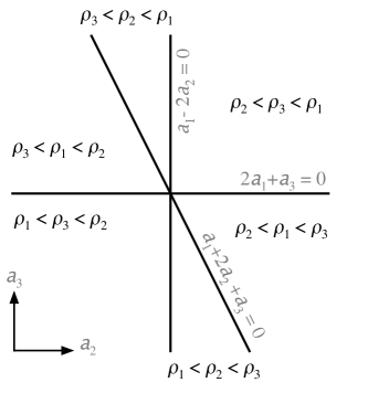
Figure 6: Section at $a_{1}=0$ of $(a_{1},a_{2},a_{3})$ parameter space, showing ordering of real parts of eigenvalues.

Remark 5.3.

Suppose arrows have range 0, 1, 2, but not 3. Then the above analysis applies with $a_{3}=0$. The transitions occur when

$$\rho_{0}=\rho_{1}: a_{1}+2a_{2}=0$$

$$\rho_{0}=\rho_{2}: a_{1}=0$$

$$\rho_{1}=\rho_{2}: a_{1}-2a_{2}=0$$

and again all possible orderings can occur. Thus connections of all ranges are not necessary to ensure that all possible orderings can occur.

5.3 Ordering of Eigenvalues

When seeking possible orderings of the eigenvalues, the geometric approach of Example 5.2 is too complicated in general. However, we can prove one useful result: If a $\mathbb{Z}_{n}$-symmetric network has couplings of all possible ranges, its admissible ODEs admit any ordering of the real parts of eigenvalues. In particular, any oscillatory mode can be the first bifurcation for a suitable admissible/equivariant ODE.

To prove this we begin with some standard concepts from ring theory, and make some important, though obvious and pedantic, distinctions.

Let $t$ be an indeterminate. The polynomial ring $\mathbb{C}[t]$ consists of all polynomial expressions

$$p=p_{0}+p_{1}t+p_{2}t^{2}+\cdots+p_{k}t^{k}\qquad(p_{j}\in\mathbb{C},0\leq j\leq k)$$ (18)

added and multiplied in the obvious manner. The corresponding polynomial function has the form

$$z\mapsto p_{0}+p_{1}z+p_{2}z^{2}+\cdots+p_{k}z^{k}\qquad(z\in\mathbb{C})$$

We can identify this function with $p$, writing $z\mapsto p(z)$, and use the same term ‘polynomial’ for both the formal expression and the corresponding function.

The ring $\mathbb{C}[t]$ contains the subring

$$\mathbb{R}[t]=\{p:p_{0},p_{1},\ldots,p_{k}\in\mathbb{R}\}$$

of polynomials with real coefficients.

The complex conjugate $\bar{p}$ of $p$ is defined by

$$p=\bar{p}_{0}+\bar{p}_{1}t+\bar{p}_{2}t^{2}+\cdots+\bar{p}_{k}t^{k}\in\mathbb{C}[t]$$

where the bar denotes the usual conjugate in $\mathbb{C}$. An obvious but important feature is that when $z\in\mathbb{C}$, then in general $\bar{p}(z)$ is not the same as $\overline{p(z)}$. In fact,

$$\overline{p(z)}=\bar{p}(\bar{z})\qquad(z\in\mathbb{C})$$

and the two sides can differ.

The next result is trivial but crucial:

Lemma 5.4.

If $p\in\mathbb{C}[t]$ then $p+\bar{p}\in\mathbb{R}[t]$.

Proof.

With coefficients $p_{j}$ as in (18),

$$(p+\bar{p})(t)=p(t)+\bar{p}(t)=\sum_{j=0}^{k}(p_{j}+\bar{p}_{j})t^{j}\in\mathbb{R}[t]$$

since $p_{j}+\bar{p}_{j}\in\mathbb{R}$. ∎

With nodes $0,1,\ldots,n-1$ define

$$N=\lfloor n/2\rfloor$$

Then the real parts of the eigenvalues are $\mu_{0},\ldots,\mu_{N}$, and each singleton or conjugate pair occurs exactly once in this list. We now prove:

Theorem 5.5.

Let $\alpha_{0},\ldots,\alpha_{N}\in\mathbb{R}$. Then there exists a polynomial $\phi(t)$ of degree $n$ in $\mathbb{R}[t]\subseteq\mathbb{C}[t]$ such that

$$\phi(\zeta^{j})=\alpha_{j}=\phi(\bar{\zeta}^{j})\qquad(0\leq j\leq N)$$ (19)

Proof.

First observe that if $n$ is even then $\zeta^{N}=\bar{\zeta}^{N}$ so (19) imposes $n$ conditions on $\phi$. By polynomial interpolation there is a polynomial $\psi\in\mathbb{C}[t]$ such that

$$\psi(\zeta^{j})=\mbox{\footnotesize$\frac{1}{2}$}\alpha_{j}=\psi(\bar{\zeta}^{j})\qquad(0\leq j\leq N)$$

The coefficients of $\psi$ need not be real, however, so we define

$$\phi=\psi+\bar{\psi}$$

which lies in $\mathbb{R}[t]$ by Lemma 5.4. Now, for $0\leq j\leq N$,

$$\phi(\zeta^{j})=\psi(\zeta^{j})+\bar{\psi}(\zeta^{j})=\psi(\zeta^{j})+\overline{\psi(\bar{\zeta}^{j})}=\mbox{\footnotesize$\frac{1}{2}$}\alpha_{j}+\mbox{\footnotesize$\frac{1}{2}$}\alpha_{j}=\alpha_{j}$$

$$\phi(\bar{\zeta}^{j})=\psi(\bar{\zeta}^{j})+\psi(\zeta^{j})=\psi(\bar{\zeta}^{j})+\overline{\psi(\zeta^{j})}=\mbox{\footnotesize$\frac{1}{2}$}\alpha_{j}+\mbox{\footnotesize$\frac{1}{2}$}\alpha_{j}=\alpha_{j}$$

as required. ∎

Corollary 5.6.

The real parts of the eigenvalues of $L$ can occur in any order for suitable choices of the connection strengths $a_{j}$.

Proof.

Let $\pi$ be any permutation of $\{0,1,\ldots N\}$. Set $\alpha_{j}=-\pi(j)$ in Theorem 5.5 and let the $a_{j}$ in $L$ be the coefficients of the resulting polynomial $\phi\in\mathbb{R}[t]$. Then

$$\Re(\mu_{j})<\Re(\mu_{l})\iff\alpha_{j}>\alpha_{l}$$

∎

This result also proves that, generically, the eigenvalues are all simple and there are no imaginary ones except $\pm\mathrm{i}\omega$. Thus these nondegeneracy conditions for Hopf bifurcation hold generically. The remaining nondegeneracy condition is the eigenvalue crossing condition, which is generic since it can be arranged by adding the equivariant and admissible term $\alpha x$ to the ODE, where $\alpha$ is small.

5.4 Direction of Rotation

An issue that has already been raised concerns the direction in which a rotating wave solution rotates. The $H/K$ classification does not distinguish these; indeed, for (say) $n=5$ all rotating waves have $H=\mathbb{Z}_{5},K={\bf 1}$, but there are four distinct phase patterns with phase shifts $T/5,2T/5,3T/5,4T/5$. These occur in pairs $\pm 1/5$ and $\pm 2/5$. For each irreducible representation over $\mathbb{R}$, precisely one from each pair can occur.

The twisted isotropy subgroup $H^{\phi}$ of (11) does distinguish the rotation directions, Because $H^{\theta}$ and $H^{-\theta}$ are generally different. However, in $\mathbb{Z}_{n}$-equivariant Hopf bifurcation the same critical eigenspace $U_{k}=\Re(V_{k}+V_{n-k})$ supports only one phase pattern, which may rotate in either direction depending on the admissible ODE. We give a criterion to decide which of them occurs.

Assume there is a Hopf bifurcation whose critical eigenspace corresponds to the complex conjugate pair of eigenvectors $v_{k}$ and $v_{n-k}$, where $k\neq 0$ and if $n$ is even, $k\neq n/2$. The eigenvalues are generically simple, so the standard Hopf Theorem predicts a unique branch of periodic states. The Equivariant Hopf Theorem adds information about the spatio-temporal symmetry of the solution along this branch. The branch consists of rotating waves, in which the $n$-cycle $\alpha$ produces a phase shift of $\pm kT/n$, so that

$$x_{j+1}(t)=x_{j}(t\pm\frac{kT}{n})$$ (20)

In this case the oscillation at node $j+1$ is phase-shifted by $\mp\frac{2k\pi}{T}$ from the oscillation at node $j$, so the signs are reversed.

The solution branch therefore consists of either a clockwise rotating wave, when the sign in (20) is negative, or an anticlockwise rotating wave, when the sign in (20) is positive. A natural question is: Which sign occurs for a given admissible ODE?

A clockwise rotating wave for $k$ can also be interpreted as an anticlockwise one for $n-k$. But it differs from an anticlockwise one for $k$, so the question is meaningful.

We show that the answer depends on the sign of the imaginary part of the critical eigenvalue. The proof is based on [38, Proposition 4.21], which is the special case $n=3$.

Recall from (17) that the eigenvalues are

$$\mu_{k}=a_{0}+a_{1}\zeta^{k}+a_{2}\zeta^{2k}+\cdots+a_{n-1}\zeta^{(n-1)k}$$ (21)

Write $\mu_{k}=\rho_{k}+\mathrm{i}\sigma_{k}$. Now

$$\Re(\mu_{k}) = \sum_{j=0}^{n}a_{j}\cos\frac{2kj\pi}{n}=\rho_{k}$$

$$\Im(\mu_{k}) = \sum_{j=0}^{n}a_{j}\sin\frac{2kj\pi}{n}=\sigma_{k}$$

At Hopf bifurcation $\rho_{k}=0$, so $\mu_{k}=\mathrm{i}\sigma_{k}$. Moreover, $\sigma_{k}\neq 0$.

Theorem 5.7.

Let $0\leq k\leq N$. Consider Hopf bifurcation with critical eigenspace given by the eigenvalue $\mu_{k}$. The the direction of rotation is clockwise if and only if $\sigma_{k}<0$, and anticlockwise if and only if $\sigma_{k}>0$.

Proof.

Use the eigenvector basis $\{u_{k},u_{n-k}\}$ over $\mathbb{C}$ on the complexified critical eigenspace. Then

$$\alpha=\left[\begin{array}[]{ccccccccccccccccccccccccr}\zeta^{k}&0\\ 0&\zeta^{n-k}\end{array}\right]\qquad L|_{E}=\left[\begin{array}[]{ccccccccccccccccccccccccr}\mathrm{i}\sigma&0\\ 0&-\mathrm{i}\sigma\end{array}\right]$$

The direction of rotation is determined by the kernel of the action of the twisted group $\langle(\alpha,\theta)\rangle\subseteq\mathbb{Z}_{n}\times{\bf S}^{1}$, when $\theta$ is the phase shift (either $\frac{2\pi k}{T}$ or $-\frac{2\pi k}{T}$). That is, we need to know whether $\alpha={\mathrm{e}}^{2\pi kT/n}$ or $\alpha={\mathrm{e}}^{-2\pi kT/n}$ on $E$.

The ${\bf S}^{1}$-action is given by $\theta$ acts as $\exp(L|_{E}\theta)$. This has matrix

$$\exp(L|_{E}\theta)=\left[\begin{array}[]{ccccccccccccccccccccccccr}{\mathrm{e}}^{\mathrm{i}\sigma}&0\\ 0&{\mathrm{e}}^{-\mathrm{i}\sigma}\end{array}\right]$$

so either

$$\sigma = \sin\frac{2k\pi}{n}$$

$$\sigma = -\sin\frac{2k\pi}{n}$$

Now

$$\sin\frac{2k\pi}{n}>0 1\leq k\leq N$$ when

$$\sin\frac{2k\pi}{n}<0 N+1\leq k\leq n-1$$ when

We can consider only the case $1\leq k\leq N$, to avoid the ambiguity mentioned above. Thus the phase shift is given by the sign of $\sigma$. If $\sigma>0$ then $\alpha$ identifies with a phase shift of $+kT/n$, and if $\sigma<0$ then $\alpha$ identifies with a phase shift of $-kT/n$.

∎

5.5 Stability

Since generic $\mathbb{Z}_{n}$-equivariant Hopf bifurcation occurs at a simple eigenvalue, the usual stability conditions for Hopf bifurcation without symmetry apply: see [47, Chapter 1 Section 4] or [35, Chapter VIII Section 4]. Assume that the branch of equilibria concerned is linearly stable for $\lambda<\lambda_{0}$, so the first bifurcation is the Hopf bifurcation under discussion. Then supercritical branches, which exist for $\lambda>\lambda_{0}$ and $|\lambda-\lambda_{0}|$ small, are stable near the bifurcation point, whereas subcritical branches, which exist for $\lambda<\lambda_{0}$ and $|\lambda-\lambda_{0}|$ small, are unstable. (Degenerate cases may be neither supercritical nor subcritical. The results of [32] then apply.)

The direction of branching can be computed from the Liapunov-Schmidt reduction or other dimension reduction methods such as Poincaré-Birkhoff normal form or centre manifold reduction. See [47, Chapter 1 Sections 3–6] [35, Chapter VIII Proposition 3.3]. Since admissible maps contain many quadratic and cubic terms, it seems likely that the generic behaviour is nondegenerate, with either a supercritical branch or a subcritical one.

6 Multidimensional Node Spaces

We sketch how the results for 1-dimensional node spaces generalise to $l$-dimensional node spaces $\mathbb{R}^{l}$ for $l>1$. The state space is then $R^{ln}$, which we can think of as the tensor product $R^{l}\otimes\mathbb{R}^{n}$. The Jacobian has the form $J=P\otimes I+Q\otimes A$ for arbitrary $l\times l$ matrices $P,Q$.

Lemma 6.1.

If $y$ is an eigenvector of $P+\zeta^{k}Q$ with eigenvalue $\rho$, then $y\otimes v_{k}$ is an eigenvector of $J$ with eigenvalue $\rho$.

A similar statement holds for generalised eigenvectors.

Proof.

Suppose that $(P+\zeta^{k}Q)y=\rho y$. Then

$$J(y\otimes v_{k}) = (P\otimes I+Q\otimes A)(y\otimes v_{k})$$

$$= Py\otimes v_{k}+Qy\otimes Av_{k}$$

$$= Py\otimes v_{k}+Qy\otimes\zeta^{k}v_{k}$$

$$= (P+\zeta^{k}Q)(y\otimes v_{k})$$

The case of a generalised eigenvector is similar. ∎

Corollary 6.2.

The set of eigenvalues of $J$ is the union of the sets of eigenvalues of all matrices $P+\zeta^{k}Q$ for $0\leq k\leq n-1$.

Hopf bifurcation then occurs when $P+\zeta^{k}Q$ has a non-zero purely imaginary eigenvalue. Since $l\geq 2$ this is always possible for suitable $P,Q$, so the cases $k=0$ and $k=n/2$ ($n$ even) are no longer excluded. Provided suitable nondegeneracy conditions hold, the oscillations for $k=0$ are synchronous; for $k=n/2$, neighbouring nodes are half a period out of phase; the rest are discrete rotating waves with the same patterns as in the case $l=1$.

The strong constraints on the first bifurcation no longer apply. For example, when $n=5$ and $l=1$ the only Hopf bifurcation that can be the first occurs for $k=2$, and $k=1$ is not possible. When $l=2$, however, the eigenvalues of $P+\zeta Q$ can be the first critical eigenvalues. For example, suppose that

$$Q=\left[\begin{array}[]{ccccccccccccccccccccccccr}1&0\\ 0&2\end{array}\right]\qquad P=\left[\begin{array}[]{ccccccccccccccccccccccccr}\lambda&0\\ 0&\lambda\end{array}\right]$$

Then the eigenvalues of $\zeta^{k}Q$, numerically, are

$$k=0 0.5+2.39792\,\mathrm{i}\qquad 0.5-2.39792\,\mathrm{i}$$

$$k=1 -2.12604+1.21652\,\mathrm{i}\qquad 2.43506-0.265468\,\mathrm{i}$$

$$k=2 -1.81397-1.64606\,\mathrm{i}\qquad 1.00495+2.23385\,\mathrm{i}$$

with largest real part $2.43506$ when $k=1$. Thus the eigenvalues of $\lambda I+\zeta^{k}Q$ are these with $\lambda$ added, and occur in the same order of real parts. As $\lambda$ increases from (say) -3, the first bifurcation occurs at $\lambda=-2.43506$, which is a Hopf bifurcation for the $k=1$ mode of oscillation.

In this example, all local bifurcations are Hopf.

7 Symmetric Bidirectional Rings

Any $\mathbb{D}_{n}$-symmetric bidirectional ring is a special case of the general $\mathbb{Z}_{n}$-group network unidirectional ring with couplings of all ranges, discussed in Section 5.2. To obtain $\mathbb{D}_{n}$ symmetry we require the input arrows from nodes $i\pm j$ to node $i$ have the same arrow-type, hence the same connection strength at criticality.

We can therefore read off the linear results—such as the eigenvalues and eigenvectors—for bidirectional rings from those for the general $\mathbb{Z}_{n}$-group network unidirectional ring. In particular, in (16) we now have $a_{j}=a_{n-j}$ for $0\leq j\leq n-1$. With 1-dimensional node spaces, the eigenvalues are now

$$\mu_{k}=a_{0}+a_{1}(\zeta^{k}+\zeta^{(n-1)k})+a_{2}(\zeta^{2k}+\zeta^{(n-2)k})+\cdots$$ (22)

where now $k$ ranges from $0$ to $\lceil n/2\rceil$.

All eigenvalues other than those for $k=0$ and $k=n/2$ when $n$ is even are now double. However, the Equivariant Hopf Theorem comes to our rescue by splitting off simple eigenvalues for $\mathbb{C}$-axial subgroups. The main new feature is the occurrence of new $\mathbb{C}$-axial subgroups, not generically present for $\mathbb{Z}_{n}$ symmetry [37, 38, 39]. For example, when $n=3$ these $\mathbb{C}$-axial subgroups are $\mathbb{Z}_{2}$ subgroups generated by reflection in a symmetry axis, and the oscillations have on of the following forms:

$$x(t) = (u(t),u(t),v(t))$$

$$x(t) = (u(t),u(t+\frac{T}{2}),v(t))$$

where $T$ is the period and $v(t)$ has period $\frac{T}{2}$. This called a multirhythm state [38, 39, 42]. Conditions for these states to be stable are stated in [35, 42] in terms of the Liapunov-Schmidt reduced function.

7.1 Exotic Patterns

In [7, Lemma 4.6, Corollary 4.9] it is proved that for $\mathbb{Z}_{n}$- and $\mathbb{D}_{n}$-symmetric rings with couplings of all ranges, every balanced colouring is an orbit colouring; that is, determined by the fixed-point subspace of a subgroup of the symmetry group. The proof of Lemma 4.6 in that paper omits one case, as noted in [39, Proposition 26.7], but when this case is taken into account the result that every balanced colouring is an orbit colouring in these networks remains valid [39, Propositions 26.6, 26.7]. However, special conditions on symmetric ring networks can lead to different balanced colourings. For example, [34] observe that in a 12-node bidirectional ring with both nearest-neighour and next-nearest-neighour connections, if these connections have the same arrow-type, there exists an exotic synchrony pattern, not given by a subgroup of the symmetry group $\mathbb{D}_{12}$.

     

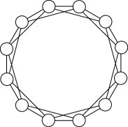
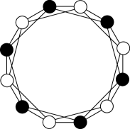
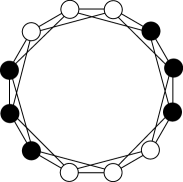
Figure 7: Left: 12-node bidirectional ring with NN and NNN coupling, assumed identical. Middle: Orbit colouring for $v_{6}$. Right: A balanced colouring that is not an orbit colouring.

Exotic phase patterns can also occur, lifted from the corresponding quotient network. Here, the quotient has $\mathbb{Z}_{2}$ symmetry. If node spaces have dimension 2 or more, there can be oscillation patterns in which all nodes of the same colour are synchronous, but the black nodes are a half period out of phase with the white nodes. It is shown in [6, Section 6] that this pattern can occur stably as an equilibrium.

Acknowledgements

I thank Mainak Sengupta for helpful discussions on symmetries of electronic rectifier circuits. Some of the results in this paper were obtained in collaboration with Luciano Buono, Jim Collins, Benoit Dionne, Marty Golubitsky, Martyn Parker, and David Schaeffer.

References

- [1]
- [2] N. Agarwal and M.J. Field. Dynamical equivalence of network architecture for coupled dynamical systems I: asymmetric inputs, Nonlinearity 23 (2010) 1245–1268.
- [3] N. Agarwal and M.J. Field. Dynamical equivalence of network architecture for coupled dynamical systems II: general case, Nonlinearity 23 (2010) 1269–1289.
- [4] A. Albanese, L. Cheng, M. Ursino, and N.W. Chbat. An integrated mathematical model of the human cardiopulmonary system: model development, Amer. J. Physiol: Heart and Circulatory Physiol. 310 (2016); doi:10.1152/ajpheart.00230.2014.
- [5] J.C. Alexander. Patterns at primary Hopf bifurcations of a plexus of identical oscillators, SIAM J. Appl. Math. 46 (1986) 199–221.
- [6] F. Antoneli and I. Stewart. Symmetry and synchrony in coupled cell networks 1: fixed-point spaces, Internat. J. Bif. Chaos 16 (2006) 559–577.
- [7] F. Antoneli and I. Stewart. Symmetry and synchrony in coupled cell networks 2: group networks, Internat. J. Bif. Chaos 17 (2007) 935–951.
- [8] D.G. Aronson, M. Golubitsky, and J. Mallet-Paret. Ponies on a merry-go-round in large arrays of Josephson junctions, Nonlinearity 4 (1991) 903–910.
- [9] A. Atiya and P. Baldi. Oscillations and synchronizations in neural networks: an exploration of the labelling hypothesis, Int. J. Neural Syst. 1 (1989) 103–124.
- [10] A. Asgari-Targhi and E.B. Klerman. Mathematical modeling of circadian rhythms, Wiley Interdiscip. Rev. Syst. Biol. Med. 11 (2019) e1439; doi:10.1002/wsbm.1439.
- [11] N.M. Awal, I.R. Epstein, T.J. Kaper, and T. Vo. Symmetry-breaking rhythms in coupled, identical fast–slow oscillators, Chaos 33 (2023) 011102.
- [12] J.S. Bay and H. Hemami. Modeling of a neural pattern generator with coupled nonlinear oscillators, IEEE Trans. Biomed. Eng. 34 (1987) 297–306.
- [13] P.-L. Buono and M. Golubitsky. Models of central pattern generators for quadruped locomotion: I. primary gaits, J. Math. Biol. 42 (2001) 291–326.
- [14] O. Buse and R. Pérez. Dynamical properties of the repressilator model, Phys. Rev. E 81 (2010) 066206.
- [15] A. Chenciner and R. Montgomery. A remarkable periodic solution of the three-body problem in the case of equal masses, Ann. Math. 152 (2000) 881–901.
- [16] G. Cicogna. Symmetry breakdown from bifurcations, Lettere al Nuovo Cimento 31 (1981) 600–602.
- [17] J.J. Collins and I. Stewart. Coupled nonlinear oscillators and the symmetries of animal gaits, J. Nonlin. Sci. 3 (1993) 349–392.
- [18] J.J. Collins and I. Stewart. A group-theoretic approach to rings of coupled biological oscillators, Biol. Cybern. 71 (1994) 95–103.
- [19] L. DeVille and E. Lerman. Dynamics on networks of manifolds, SIGMA 11 (2015); arXiv:1208.1513v4 [math.DS] 2015.
- [20] A.P.S. Dias and I. Stewart. Hopf bifurcation on a simple cubic lattice, Dyn. Stab. Sys. 14 (1999) 3–55.
- [21] A. Díaz-Guilera and A. Arenas. Phase patterns of coupled oscillators with application to wireless communication, in: Bio-Inspired Computing and Communication. BIOWIRE 2007 (eds. P. Lió , E. Toneki, J. Crowcroft, and D.C. Verma), Lect. Notes in Comp. Sci. 5151, Springer, Berlin 2008, 184–191.
- [22] B. Dionne, M. Golubitsky, M. Silber, and I. Stewart. Time-periodic spatially-periodic planforms in Euclidean equivariant PDE, Phil. Trans. Roy. Soc. London A 352 (1995) 125–168.
- [23] V.L. Dunin-Barkovskii. Fluctuations in the level of activity in simple closed neurone chains, Biophysics 15 (1970) 396–401.
- [24] M.B. Elowitz and S. Leibler. A synthetic oscillatory network of transcriptional regulators, Nature 403 (2000) 335–338.
- [25] T. Endo and S. Mori. Mode analysis of a ring of a large number of mutually coupled van der Pol oscillators, IEEE Trans. Circuits Syst. 25 (1978) 7–18.
- [26] G.B. Ermentrout. The behavior of rings of coupled oscillators, J. Math. Biool. 23 (1985) 55–74.
- [27] J.R. Espinoza. Inverters, in: Power Electronics Handbook (3rd ed.) (ed. M.H. Rashid), Elsevier, Amsterdam 2011, 357–408.
- [28] N. Filipski and M. Golubitsky. The abelian Hopf mod theorem, SIAM J. Appl. Dynam. Sys. 9 (2010) 283–291.
- [29] W.O. Friesen and G.S. Stent. Neural circuits for generating rhythmic movements, Anuu. Rev. Biophys. Bioeng. bf 7 (1978) 37–61.
- [30] J.B. Furness. The Enteric Nervous System, Blackwell, Oxford 2008.
- [31] L. Glass and R.E. Young. Structure and dynamics of neural network oscillators, Brain Res. 179 (1979) 207–218.
- [32] M. Golubitsky and W.F. Langford. Classification and unfoldings of degenerate Hopf bifurcations, J. Diff. Eqns. 41 (1981) 375–415.
- [33] M. Golubitsky, L. Matamba Messi, and L. Spardy. Symmetry types and phase-shift synchrony in networks, Physica D 320 (2016) 9–18.
- [34] M. Golubitsky, M. Nicol, and I. Stewart. Some curious phenomena in coupled cell networks, J. Nonlinear Sci. 14 (2004) 207–236.
- [35] M. Golubitsky and D.G. Schaeffer. Singularities and Groups in Bifurcation Theory I, Applied Mathematics Series 51, Springer, New York 1985.
- [36] M. Golubitsky and I. Stewart. Hopf bifurcation in the presence of symmetry, Arch. Rational Mech. Anal. 87 (1985) 107–165.
- [37] M. Golubitsky and I. Stewart. Hopf bifurcation with dihedral group symmetry: coupled nonlinear oscillators, in Multiparameter Bifurcation Theory (eds. M. Golubitsky and J. Guckenheimer), Proceedings of the AMS-IMS-SIAM Joint Summer Research Conference, July 1985, Arcata; Contemporary Math. 56, Amer. Math. Soc., Providence RI 1986, 131–173.
- [38] M. Golubitsky and I. Stewart. The Symmetry Perspective: from equilibria to chaos in phase space and physical space, Progress in Mathematics 200, Birkhäuser, Basel 2002.
- [39] M. Golubitsky and I. Stewart. Dynamics and Bifurcation in Networks, SIAM, Philadelphia, to appear.
- [40] M. Golubitsky, I. Stewart, P.-L. Buono, and J.J. Collins. A modular network for legged locomotion, Physica D 115 (1998) 56–72.
- [41] M. Golubitsky, I. Stewart, J.J. Collins, and P.-L. Buono. Symmetry in locomotor central pattern generators and animal gaits, Nature 401 (1999) 693–695.
- [42] M. Golubitsky, I. Stewart, and D.G. Schaeffer. Singularities and Groups in Bifurcation Theory II, Applied Mathematics Series 69, Springer, New York 1988.
- [43] M. Golubitsky, I. Stewart, and A. Török. Patterns of synchrony in coupled cell networks with multiple arrows, SIAM J. Appl. Dynam. Sys. 4 (2005) 78–100.
- [44] S. Grillner and P. Wallén. Central pattern generators for locomotion, with special reference to vertebrates, Annu. Rev. Neurosci. 8 (1985) 233–261.
- [45] J. Guckenheimer and P. Holmes. Nonlinear Oscillations, Dynamical Systems, and Bifurcations of Vector Fields, Springer, New York 1983.
- [46] V.S. Gurfinkel and M.L. Shik. The control of posture and locomotion, in: Motor Control (eds. A.A. Gydikov, N.T. Tankov, and D.S. Kozarov), Plenum, New York 1973, 217–234.
- [47] B.D. Hassard, N.D. Kazarinoff, and Y.-H. Wan. Theory and Applications of Hopf Bifurcation, London Math. Soc. Lecture Notes 41, Cambridge University Press, Cambridge 1981.
- [48] F.C. Hoppensteadt. An Introduction to the Mathematics of Neurons, Cambridge University Press, Cambridge 1986.
- [49] A.J. Ijspeert. Central pattern generators for locomotion control in animals and robots: A review, Neural Networks 21 (2008) 642–653.
- [50] V. In, A. Kho, P. Longhini, J.D. Neff, A. Palacios, and P.-L. Buono. Meet ANIBOT: the first biologically-inspired animal robot, Internat. J. Bif. Chaos to appear.
- [51] H.G.E. Kadji, J.B.C Orou, and P. Woafo. Spatiotemporal dynamics in a ring of mutually coupled self-sustained systems, Chaos 17 (2007) 033109.
- [52] A. Kerfourn, L. Laval, and C. Letellier. Relation between synchronization of a ring of coupled Rössler systems and observability, ATEC Web of Conferences 1 (2012) 07001.
- [53] A. Kouda and S. Mori. Analysis of a ring of mutually coupled van der Pol oscillators with coupling delay, IEEE Trans. Circuits Syst. 28 (1981) 247–253.
- [54] A. Lasota and J.A. Yorke. The generic property of existence of solutions of differential equations in Banach space, J. Diff. Eq. 13 (1973) 1–12.
- [55] Y.S. Lee and M.H.L Chow. Diode rectifiers, in: Power Electronics Handbook (3rd ed.) (ed. M.H. Rashid), Elsevier, Amsterdam 2011, 149–181.
- [56] D.A. Linkens, I. Taylor, and H.L. Duthie. Mathematical modeling of the colorectal myoelectrical activity in humans, IEEE Trans. Biomed. Eng.23 (1976) 101–110.
- [57] K. Markus and Y. Serhiy. Bifurcation analysis of delay-induced patterns in a ring of Hodgkin–Huxley neurons, Phil. Trans. R. Soc. A. 371 (2013) 20120470.
- [58] K.R. Meyer. Periodic solutions of the -body problem, J. Diff. Eq. 39 (1981) 2–38.
- [59] J. Montaldi, R.M. Roberts, and I. Stewart. Periodic solutions near equilibria of symmetric Hamiltonian systems, Phil. Trans. R. Soc. Lond. A 325 (1988) 237–293.
- [60] J. Montaldi, R.M. Roberts, and I. Stewart. Existence of nonlinear normal modes of symmetric Hamiltonian systems, Nonlinearity 3 (1990) 695–730.
- [61] J. Montaldi and K. Steckles. Classification of symmetry groups for planar -body choreographies, Forum of Mathematics, Sigma 1 (2013) e5; doi:10.1017/fms.2013.5.
- [62] I. Morishita and A. Yajima. Analysis and simulation of networks of mutually inhibiting neurons, Kybernetik 11 (1972) 154–165.
- [63] J.P. Pade, S. Yanchuk, and L. Zhao. Pattern recognition in a ring of delayed phase oscillators, arXiv:1408.4666 (2014).
- [64] P. Perlikowski, S. Yanchuk, O.V. Popovych, and P.A. Tass. Periodic patterns in a ring of delay-coupled oscillators, Phys. Rev. E 82 (2010) 036208.
- [65] P. Perlikowski, S. Yanchuk, M. Wolfrum, A. Stefanski, P. Mosiolek, and T. Kapitaniak. Routes to complex dynamics in a ring of unidirectionally coupled systems, Chaos 20 (2010) 013111.
- [66] C.M. Pinto and A.R. Carvalho. Strange patterns in one ring of Chen oscillators coupled to a ‘buffer’ cell, Journal of Vibration and Control 22 (2016) 3267–3295.
- [67] N.V. Pozin and Y.A. Shulpin. Analysis of the work of auto-oscillatory neurone junctions, Biophysics 15 (1970) 162–171.
- [68] Z. Qu, G. Hu, A. Garfinkel, and J.N.Weiss. Nonlinear and stochastic dynamics in the heart, Phys Rep. 543 (2014 ) 61–162.
- [69] B. Rahman, Y.N. Kyrychko, and K.B. Blyuss. Dynamics of unidirectionally-coupled ring neural network with discrete and distributed delays, J. Math. Biol. 80 (2020) 1617–1653.
- [70] M. Roberts, J.W. Swift, and D. Wagner. The Hopf bifurcation on a hexagonal lattice, in Multiparameter Bifurcation Theory (eds. M. Golubitsky and J. Guckenheimer), Proceedings of the AMS-IMS-SIAM Joint Summer Research Conference, July 1985, Arcata; Contemporary Math. 56, Amer. Math. Soc., Providence RI 1986, 283–318.
- [71] A.I. Selverston. A consideration of invertebrate central pattern generators as computational data bases, Neural Networks 1 (1988) 109–117.
- [72] I. Stewart. Symmetry methods in collisionless many-body problems, J. Nonlin. Sci 6 (1996) 543–563.
- [73] I. Stewart, M. Golubitsky, and M. Pivato. Symmetry groupoids and patterns of synchrony in coupled cell networks, SIAM J. Appl. Dynam. Sys. 2 (2003) 609–646.
- [74] S. Smale. Differentiable dynamical systems, Bull. Amer. Math. Soc. 73 (1967) 747–817.
- [75] G. Szézkely. Logical network for controlling limb movements in Urodela, Acta. Physiol. Acad. Sci. Hung. 27 (1965) 285–289.
- [76] A.M. Turing. The chemical basis of morphogenesis, Phil. Trans. R. Soc. London B 237 (1952) 37–72.
- [77] A. Vanderbauwhede. Local Bifurcation and Symmetry. Habilitation Thesis, Rijksuniversiteit Gent 1980.
- [78] C.R.S. Williams, F. Sorrentino, T.E. Murphy, and R. Roy. Synchronization states and multistability in a ring of periodic oscillators: Experimentally variable coupling delays, Chaos 23 (2013) 043117.
- [79] R. Yamapi and R.S. Mackay. Stability of synchronization in a shift-invariant ring of mutually coupled oscillators, Discrete and Continuous Dynam. Syst. B 10 (2008); doi: 10.3934/dcdsb.2008.10.973.