Semi-on-Demand Hybrid Transit Route Design with Shared Autonomous Mobility Services

Abstract

This study examines the route design of a semi-on-demand hybrid route directional service in the public transit network, offering on-demand flexible route service in low-density areas and fixed route service in higher-density areas with Shared Autonomous Mobility Service (SAMS). The study develops analytically tractable cost expressions that capture access, waiting, and riding costs for users, and distance-based operating and time-based vehicle costs for operators. Two formulations are presented for strategic and tactical decisions in flexible route portion, fleet size, headway, and vehicle size optimization, enabling the determination of route types between fixed, hybrid, and flexible routes based on demand, cost, and operational parameters. The practical applications and benefits of semi-on-demand feeders are demonstrated with numerical examples and a large-scale case study in the Chicago metropolitan area. Findings reveal scenarios in which flexible route portions serving passengers located further away reduce total costs, particularly user costs. Lower operating costs in lower-demand areas favor more flexible routes, whereas higher demand densities favor more traditional line-based operations. On two studied lines, a current cost forecast favors smaller vehicles with flexible routes, but operating constraints and higher operating costs would favor bigger vehicles with hybrid routes. The study provides an analytical tool to design SAMS as directional services and transit feeders, and tractable continuous approximation formulations for future research in transit network design.

Keywords semi-on-demand  $\cdot$ transit feeder  $\cdot$ shared autonomous mobility service  $\cdot$ transit design  $\cdot$ flexible route

1 Introduction

1.1 Motivation

Mobility, a cornerstone of socio-economic well-being, is often unevenly distributed due to public transit systems’ inconsistent availability, accessibility, and quality. One of the key hurdles limiting transit access outside city centers is the first-mile-last-mile problem — from a user perspective, public transit is unattractive if reaching it requires walking for an excessive distance from one’s origin or to the final destination. From an operator perspective, line-based transit operations are often cost-inefficient in low-density areas. Taxis and rideshare services could be convenient ways to plug this gap but are not economical nor socially desirable from a congestion or environmental standpoint. Furthermore, long-term trends, such as suburbanization, and more recent trends associated with the COVID-19 pandemic, such as reduced service and increased prevalence of remote/hybrid work (Tahlyan et al. 2022), have greatly decreased transit ridership. Poor accessibility deters many travelers from relying on transit and makes driving their private vehicles the sole feasible mobility option, despite its higher costs for users (fuel and maintenance), society (delay due to congestion and space requirements for parking), and the environment (15% of global carbon emissions are contributed by road transport (Ritchie 2020)) relative to transit.

Autonomous vehicles (AVs) could potentially alleviate these mobility concerns by offering convenient point-to-point journeys (Frei, Hyland, and Mahmassani 2017). However, this convenience is predicted to induce demand, increasing total traffic volume on the road and leading to greater emissions and congestion if transit options are not also improved (Xu, Mahmassani, and Chen 2019). This work addresses these problems by exploring semi-on-demand hybrid route shared autonomous mobility service (SAMS) to plug the first-mile-last-mile gap, at least for certain situations that we will delineate. Such a system balances optimally the economies of scale of fixed route public transit with the accessibility of flexible route taxis or shared autonomous vehicles (SAVs). Addressing the first-mile-last-mile problem can expand transit coverage to provide seamless door-to-door transportation options to wider populations in a cost-effective, green, and equitable manner.

1.2 Problem Description

We consider a semi-on-demand hybrid flexible/fixed route service along a corridor (Figure 1). This entails a vehicle serving an on-demand flexible route portion for areas further from a train station/downtown (likely with more scattered demand) and — included seamlessly in the same route — a fixed route portion for areas close to a train station/downtown (likely with more concentrated demand). In the flexible route portion, there is a trade-off between saving in passengers’ access time and additional detours required for both passengers on board and vehicles. Consequently, the flexible route portion $x_{f}$ which demarcates flexible and fixed route portions is determined to minimize the total costs of users and operators at the route design level. This demarcation of fixed and flexible service areas on a particular route contributes to a clear and regular service pattern (so riders along the route would know whether to walk to a fixed stop or be picked up).

We focus on scenarios of directional demand, such as feeder service to train stations or commuter routes from suburbs to downtown. While our derivation and results cater to station/downtown-bound services, they equally apply to both inbound and outbound services. The use of AVs allows real-time change of routes in the flexible route portion that would pose operational and safety concerns to traditional human-driven buses. Additionally, this study considers the effects of operational cost reduction brought by SAVs on the flexible route portion and fleet size.

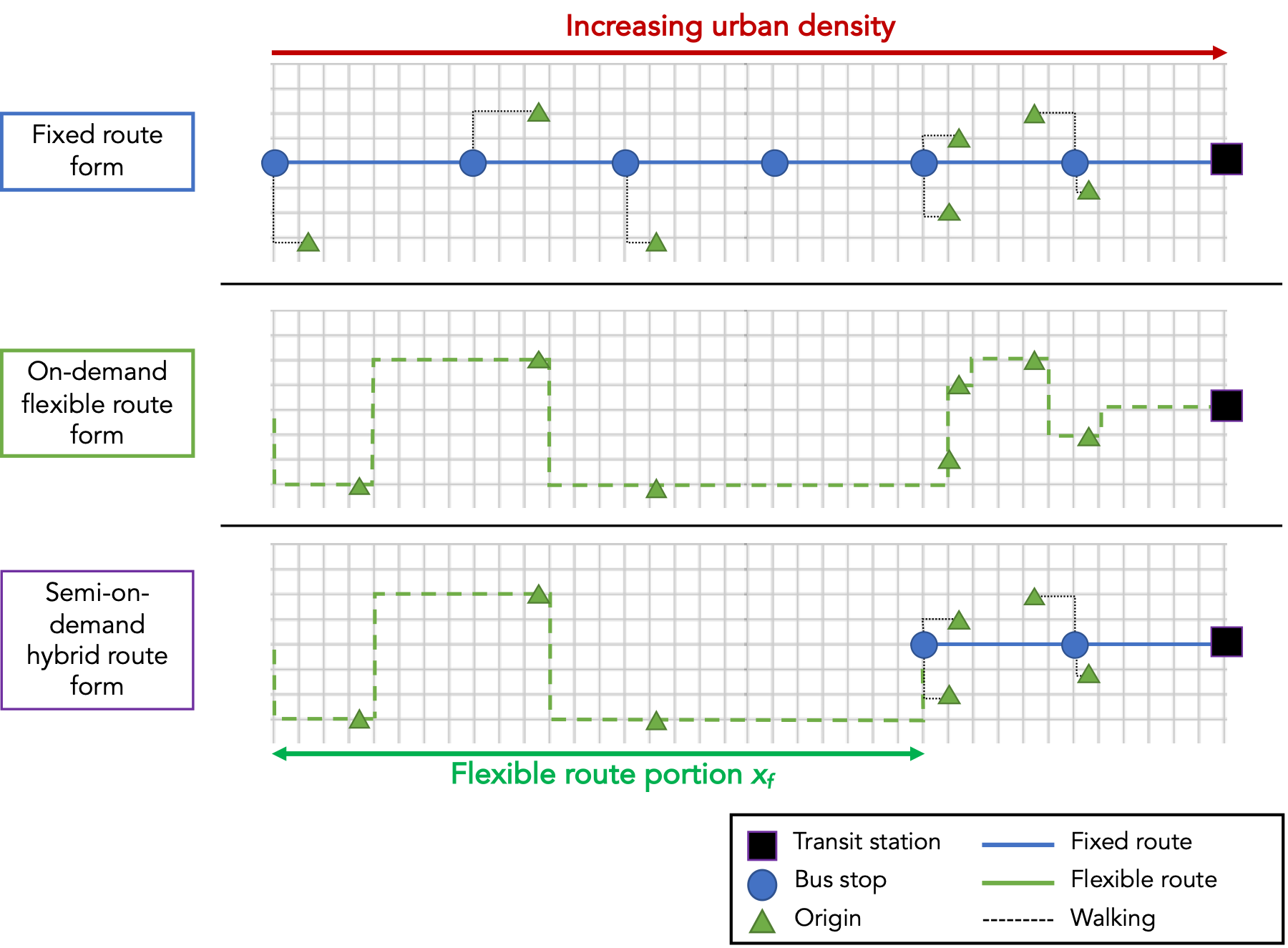
Figure 1: Illustration of Fixed Route, On-demand Flexible Route, and Semi-on-Demand Hybrid (Fixed/Flexible) Route as a Feeder Service

1.3 Objectives and Contributions

We present two cost formulations for the semi-on-demand hybrid route service: one strategic and one tactical. The strategic formulation optimizes the flexible route portion and fleet size, capturing the additional vehicle requirement for possible detours of a flexible or hybrid route. In addition to these two variables, the tactical formulation optimizes headway for new route planning to balance the effects on the waiting time and vehicle capital cost. It also considers vehicle types (sizes) in the optimization, resulting in a comprehensive model to support network planning, select vehicle and fleet sizes simultaneously, and design flexible route portions and headways.

This paper provides three key contributions.

• Conceptually, we investigate the applicability and benefits of a semi-on-demand hybrid route form with general cost formulations that also cover fixed and flexible route forms. This delineates the conditions under which each of the three route forms is optimal, supplemented with tractable cost approximations.

• Methodologically, we derive an analytical approach to determine the optimal route form and, for hybrid routes, the optimal flexible route portion and fleet size, without the need for computationally expensive simulation-based optimization. We also conduct joint numerical optimization with the headway and vehicle size. These allow efficient transit service design and sensitivity study with respect to demand, geospatial, service, and cost parameters.

• From an application standpoint, we demonstrate the benefits and applications of semi-on-demand feeders with numerical examples and a large-scale real-world case study in the Chicago metropolitan area, USA.

The paper is structured as follows: Section 2 reviews relevant literature, focusing on flexible transit service design and SAMS. We then introduce the two mathematical formulations for costs and derive optimal values for the respective decision variables in Section 3. To illustrate these formulations, we present two numerical examples in Section 4 — the first focuses on the flexible route portion and fleet size, and the second incorporates headway and vehicle size. Subsequently, a city-scale case study of feeder services in Chicago is discussed in Section 5. Finally, we conclude the paper with a summary of the findings, limitations, and future research directions in Section 6.

2 Background

2.1 Flexible Transit Route Design

Previous research efforts mainly focused on flexible/adaptive transit route designs differentiating usage of fixed route and demand-responsive transit (DRT) services. Chang and Schonfeld (1991) analytically compared fixed and one-stop flexible service and optimized fleet and vehicle sizes. Quadrifoglio and Li (2009) and Li and Quadrifoglio (2010) designed analytical models to identify the condition for switching between demand-responsive and fixed route policies that maximize service quality. Nourbakhsh and Ouyang (2012) analyzed flexible route transit systems in a corridor with continuous approximation. Rich et al. (2023) compared fixed route and demand-responsive methods as feeders for light rail transit using agent-based simulation. Other studies looked into parallel flexible routes (Chen and Nie 2017) and joint design of transit and DRT with queuing network model (Liu and Ouyang 2021) and path-based network optimization (Steiner and Irnich 2020). More recently, Martínez Mori, Speranza, and Samaranayake (2023) showed mathematically the value of flexibility brought by DRT. Calabrò et al. (2023) chose a fixed route or DRT feeder and designed the trunk service accordingly. For other recent advances in demand-responsive systems, see the survey by Vansteenwegen et al. (2022). Overall, these studies considered decisions to deploy flexible route or fixed route services. In contrast, this study explores the hybrid route, which is a continuous spectrum defined by the flexible route portion between the two service modes.

Research on semi-flexible transit systems involved various optimization strategies (see a survey by Errico et al. (2013) on earlier planning efforts). Qiu, Li, and Zhang (2014) used an analytical model and simulation to decide which curb-to-curb stops are served, aiming to minimize user costs. Galarza Montenegro, Sörensen, and Vansteenwegen (2021) proposed a demand-responsive feeder system with mandatory and optional bus stops. Zheng et al. (2019) introduced a blend of flexible and fixed routes via meeting points. Leffler et al. (2021) investigated on-demand operational policies for autonomous vehicles, showing improved waiting times on trunk routes in particular. Mishra and Mehran (2023) optimized service headway and curb-to-curb service requests using non-dominated sorting to generate a Pareto set. For stochastic approaches, Rambha, Boyles, and Waller (2016) formulated an adaptive routing problem as a finite horizon Markov decision process. Li, Lee, and Lo (2023) looked into a stochastic problem of zonal on-demand flexible bus routes. Olivos, Silva, and Vinel (2023) proposed a Markovian continuous approximation-based semi-flexible system model on a single bus operation. Other similar service models include "customized bus" with demand-based pre-designed routes (Huang et al. 2020, Abdelwahed et al. 2023), hybrid first-mile-last-mile service between shuttle and transportation network companies (TNCs) (Grahn, Qian, and Hendrickson 2022), and demand-adaptive system (Errico et al. 2021). While the previously discussed literature explored a wide range of flexible transit services, this study focuses on the proposed semi-on-demand routes, which pre-design portions of flexible and fixed routes for consistent service patterns. It combines the economies of scale and predictability of scheduled fixed routes and the door-to-door convenience of flexible routes. Additionally, most previous efforts relied on a mix of simulation, heuristics, or mixed-integer linear programming, which hinders intuitive sensitive analysis based on design parameters. This study provides an analytical approach to total cost minimization for delineating the conditions of the optimal route form (fixed/hybrid/flexible) with the optimal flexible route portion and fleet size.

2.2 Shared Autonomous Mobility Services (SAMS) in Public Transit Systems

The shared element of SAMS improves service quality and operational efficiency (Hyland and Mahmassani 2020), with their potential synergies as part of the public transit systems highlighted by Shen, Zhang, and Zhao (2018), Salazar et al. (2020), and Cortina, Chiabaut, and Leclercq (2023) in case studies of Singapore, New York, and Lyon. Badia and Jenelius (2021) designed feeder systems with AVs and studied cost with continuous approximation. Gurumurthy, Kockelman, and Zuniga-Garcia (2020) demonstrated the potential of SAVs as feeders for public transit in Austin, proposing fare benefits for transit users to increase transit coverage and reduce walking distances. Levin et al. (2019) looked into the optimal integration of SAVs and transit with continuous approximation and linear programming. Transit was only used when it reduced total system travel time. Luo, Samaranayake, and Banerjee (2021) optimized mobility-on-demand service flow, transit frequency, and pricing jointly. Ng et al. (2024) redesigned existing multimodal transit networks with SAMS as point-to-point and feeder services. Some research (e.g., Zhang, Tafreshian, and Masoud (2020), Liu, Qu, and Ma (2021), Tian et al. (2022)) investigated an evolving idea of autonomous modular transit and their roles in the overall network.

A contrasting body of research evaluated SAVs as replacements for existing transit systems. Sieber et al. (2020) proposed that autonomous mobility on demand (AMoD) could potentially replace rural trains in Switzerland, analyzing the difference in costs and service levels. Ng and Mahmassani (2023) and Volakakis, Ng, and Mahmassani (2023) showed around 20% performance improvement by replacing fixed bus routes with flexible routes in suburbs. Mo et al. (2021) analyzed the impact of dynamic adjustable supply strategies and regulations in SAV fleet size and transit headway changes on system efficiency. Cao and Ceder (2019) proposed stop-skipping with autonomous shuttles and evaluated the number of extra vehicles required.

Lastly, several researchers have sought to optimize SAV design variables, such as vehicle size (Alonso-Mora et al. 2017) and fleet size (Pinto et al. 2020, Dandl et al. 2021). Pinto et al. (2020) highlighted the need to consider waiting time in optimization, presenting a bi-level mathematical programming formulation and solution approach. Sadrani, Tirachini, and Antoniou (2022) optimized autonomous bus service frequency and vehicle size. Following the previous work (Ng and Mahmassani 2023) which assessed the attractiveness of flexible route operation with autonomous minibuses in suburbs, this study generalizes it to optimize the portion of flexible route with other parameters and variables. We determine the optimal portion between fixed route and flexible route in a continuous spectrum of hybrid routes.

3 Mathematical Formulations

This section consists of two main models. We start with the optimization of the flexible route portion $0\leq x_{f}\leq L_{x}$ (in km) and fleet size $s>0$ (in vehicle, or veh) subject to a fixed headway $H$ (in h), which allows us to set $s$ as a function of $x_{f}$. We discuss the model first with a general demand distribution, followed by specific forms under uniform and triangular distributions. It is worth noting that $x_{f}=0$ implies a fixed route, $0<x_{f}<L_{x}$ a hybrid route, and $x_{f}=L_{x}$ a flexible route. Next, we relax the fixed headway assumption and set it as a function $h(x_{f},s)$ in optimization. This accounts for the trade-off between waiting times and extra vehicle costs. We also generalize vehicle sizes where the previously constant operational and vehicle costs are functions of vehicle sizes under a capacity requirement constraint.

The general assumptions throughout this section are as follows:

1. We illustrate the service in a grid network with route running direction as the x-axis and perpendicular detours as the y-axis. Vehicles travel along the x-direction and stop by demand points in sequence, i.e., there is no backtracking.

2. The total dwell time and layover time (at the transit station) are constant; vehicles travel at a constant speed $V_{d}$ (in km/h).

3. We consider a static demand in a continuous horizon. Demand is within capacity.

4. All travelers are individuals; group size is not considered other than as a collection of independent travelers.

The notation is summarized in Table 1. Variables are denoted as small Roman characters (e.g., $x_{f}$, $s$, $b$, $h$) and constants as capital Roman characters (e.g., $L_{x}$, $H$), except for cost coefficients $\gamma$ and total demand $\Lambda$. The demand density function is $f(x)$, with its derivative as $f^{\prime}(x)$ and cumulative density function as $F(x)$. Demand and costs are on a per-hour basis.

Table 1: Summary of Notation

Symbol	Description
$\gamma_{a}$	Access cost factor
$\gamma_{o}$	Operating cost
$\gamma_{t}$	Value of time
$\gamma_{v}$	Vehicle cost
$\gamma_{w}$	Waiting cost factor
$\Lambda$	Total demand
$\lambda$	Demand density
$\lambda_{0}$	Maximum demand density (for triangular distribution)
$\overline{d_{d,y}}$	Mean detour
$\overline{t_{a}}$	Mean fixed route access time
$\rho$	Capacity buffer over demand
$b$	Vehicle size
$c$	Total cost
$c_{o,x}$	Operator cost (x-directional)
$c_{o,y}$	Operator cost (y-directional)
$c_{t,x}$	Riding cost (x-directional)
$c_{t,y}$	Riding cost (y-directional)
$c_{a}$	Access cost
$c_{v}$	Vehicle cost
$c_{w}$	Waiting cost
$f$	Demand density function
$F$	Cumulative demand density function
$f^{\prime}$	Demand density function derivative
$H$ or $h$	Headway
$L_{x}$	Total route length in the x-direction
$s$	Fleet size
$V_{d}$	Vehicle speed
$x_{f}$	Flexible route portion

3.1 Optimization of the Flexible Route Portion and Fleet Size given a Headway

3.1.1 General Form.

A general demand distribution along the x-direction is assumed, with density function $f(x)\geq 0,\forall x\in[0,L_{x}]$ (in passenger/km or pax/km) and cumulative demand function $F(x)=\int_{0}^{x}f(\tilde{x})d\tilde{x}$ (in pax). The total demand is denoted as $\Lambda=F(L_{x})$ (in pax), where $L_{x}$ (in km) is the total route length in the x-direction (without detours), so $0\leq F(x)\leq\Lambda,\forall x\in[0,L_{x}]$. We conventionally go from low- to high-density area, i.e., flexible route before fixed route, along the x-axis (see Figure 1). Demand along the y-axis is also assumed to follow a general distribution, resulting in a mean fixed route access time $\overline{t_{a}}$ (in h) and a mean detour $\overline{d_{d,y}}$ (in km). $\overline{d_{d,y}}$ is the average y-directional distance between consecutive request points along the x-direction (see more detailed discussion and approximation by Ng and Mahmassani (2023)).

In this formulation, we assume a constant headway $H$ (in h) to maintain constant waiting time and route capacity. We also ignore the fleet size integrality. (Non-integer fleet size may be used to represent operational arrangement, e.g., interlining, where vehicles are shared across routes. Furthermore, the additional complexity induced by the integrality constraints may necessitate numerical optimization methods.)

Then, to simplify the minimization problem to univariate, $s$ can be expressed as a function of $x_{f}$ by considering the cycle time divided by the headway $H$ in Eq. 3.1.1. $t_{x}$ is the x-directional travel time. $t_{y}(x_{f})$ is the y-directional total detour time in Eq. 3.1.1, based on the number of detours, i.e., demand in the flexible route portion $\int_{0}^{x_{f}}f(x)dx=F(x_{f})$, divided by $H$ for each vehicle trip and multiplied by the average detour time $\overline{d_{d,y}}/v_{d}$. $T_{l}$ is the layover time between one-way bus trips.

$$s(x_{f}) =\frac{2}{H}\left(t_{x}+t_{y}(x_{f})+T_{l}\right)$$

$$=\frac{2}{H}\left(\frac{L_{x}}{V_{d}}+\frac{H\overline{d_{d,y}}}{V_{d}}F(x_{f})+T_{l}\right)$$ (1)

$$t_{y}(x_{f}) =H\frac{\overline{d_{d,y}}}{V_{d}}\int_{0}^{x_{f}}f(x)dx$$

$$=H\frac{\overline{d_{d,y}}}{V_{d}}F(x_{f})$$ (2)

We consider total cost from a societal view from both user and operator perspectives. The objective is to minimize the total costs $c(x_{f})$ (in $) as a function of the flexible route portion $x_{f}$. $c(x_{f})$ is composed of travelers’ costs: access cost $c_{a}(x_{f})$ (for fixed route portion only), waiting cost $c_{w}$, riding costs (x-direction: $c_{t,x}$, and, for flexible route portion only, y-directional detour $c_{t,y}(x_{f})$); and distance-based operator costs: $c_{o,x}$ (in x-direction) and $c_{o,y}(x_{f})$ (y-direction, for flexible route portion only) and vehicle cost $c_{v}(s)$ as a function of the fleet size $s>0$. These costs are computed similarly to Ng and Mahmassani (2023) with reference to Newell (1979) formulation. The cost factors are the value of time $\gamma_{t}$ (in $/h), access cost factor $\gamma_{a}$ and waiting cost factor $\gamma_{w}$ (in multiples of riding cost), as well as operating cost $\gamma_{o}$ (in $/km) and vehicle cost $\gamma_{v}(s)$ (in $/veh).

The access (walking) cost $c_{a}(x_{f})$ is calculated in Eq. 3 as the product of the value of access time, $\gamma_{t}\gamma_{a}$, average access time $\overline{t_{a}}$, and number of passengers served in the fixed route portion $\Lambda-F(x_{f})$. The waiting cost $c_{w}$ in Eq. 4 is a constant equal to the product of values of waiting time $\gamma_{t}\gamma_{w}$, total number of passengers $\Lambda$, and expected waiting time (half of headway $H$).

$$c_{a}(x_{f}) =\gamma_{t}\gamma_{a}\overline{t_{a}}(\Lambda-F(x_{f}))$$ (3)

$$c_{w} =\gamma_{t}\gamma_{w}\Lambda\frac{H}{2}$$ (4)

The riding cost is separated into x-directional travel and y-directional detours. For x-directional travel, each passenger getting on the bus at $x$ needs to travel a distance of $L_{x}-x$, resulting in the total riding distances as the integral $\int_{0}^{L_{x}}f(x)(L_{x}-x)dx$. The constant x-directional riding cost $c_{t,x}$ is then its product with the value of time $\gamma_{t}$ divided by the vehicle speed $V_{d}$ in Eq. 5. For y-directional detour, each passenger getting on the bus at $x$ in the flexible portion rides the extra detours to pick up remaining passengers between $x$ and $x_{f}$ in the flexible portion $\int_{x}^{x_{f}}Hf(\tilde{x})d\tilde{x}$ (multiplied by $H$ to convert hourly demand to number of passengers per vehicle), resulting in the double integral in Eq. 6. After simplification, it is apparent that the y-directional riding cost $c_{t,y}(x_{f})$ is proportional to the square of cumulative demand function $F(x_{f})$.

$$c_{t,x} =\gamma_{t}\frac{1}{V_{d}}\int_{0}^{L_{x}}f(x)(L_{x}-x)dx$$

$$=\gamma_{t}\frac{1}{V_{d}}\int_{0}^{L_{x}}F(x)dx$$ (5)

$$c_{t,y}(x_{f}) =\gamma_{t}\int_{0}^{x_{f}}f(x)\int_{x}^{x_{f}}Hf(\tilde{x})d\tilde{x}dx\frac{\overline{d_{d,y}}}{V_{d}}$$

$$=\gamma_{t}H\frac{\overline{d_{d,y}}}{2V_{d}}F(x_{f})^{2}$$ (6)

The distance-based operating cost is also separated into x- and y-directional components. The constant x-directional operating cost $c_{o,x}$ in Eq. 7 is determined by the route length, divided by the headway $H$ to reflect the hourly frequency. In contrast, for the y-directional detour, $H$ is canceled out for $c_{o,y}(x_{f})$ in Eq. 8, i.e., the operating cost due to detours depends on the total number of detours but not the headway.

$$c_{o,x} =\gamma_{o}\frac{L_{x}}{H}$$ (7)

$$c_{o,y}(x_{f}) =\gamma_{o}\frac{1}{H}\int_{0}^{x_{f}}Hf(x)dx\overline{d_{d,y}}=\gamma_{o}\overline{d_{d,y}}F(x_{f})$$ (8)

The vehicle cost is calculated in Eq. 9 as directly proportional to the hourly vehicle cost $\gamma_{v}$ (in $/veh), to cover the marginal costs of additional vehicles.

$$c_{v}(x_{f}) =\gamma_{v}s(x_{f})=\gamma_{v}\frac{2}{H}\left(\frac{L_{x}}{V_{d}}+\frac{H\overline{d_{d,y}}}{V_{d}}F(x_{f})+T_{l}\right)$$ (9)

The total cost $c(x_{f})$ in Eq. 10 is the sum of all costs in Eq. 3-9. It enables us to determine the optimal route form analytically with Result 1 based on geospatial, cost, and operational parameters.

$$c(x_{f}) =\gamma_{t}\gamma_{a}\overline{t_{a}}(\Lambda-F(x_{f}))+\gamma_{t}\gamma_{w}\Lambda\frac{H}{2}$$

$$\quad+\gamma_{t}\frac{1}{V_{d}}\int_{0}^{L_{x}}F(x)dx+\gamma_{t}H\frac{\overline{d_{d,y}}}{2V_{d}}F(x_{f})^{2}$$

$$\quad+\gamma_{o}\frac{L_{x}}{H}+\gamma_{o}\overline{d_{d,y}}F(x_{f})$$

$$\quad+\gamma_{v}\frac{2}{H}\left(\frac{L_{x}}{V_{d}}+\frac{H\overline{d_{d,y}}}{V_{d}}F(x_{f})+T_{l}\right)$$ (10)

Result 1.

Given a fixed fleet size and a fixed headway $H$, the optimal route form that minimizes the total cost function $c(x_{f})$ in Eq. 10 is one of the following:

1. Fixed route if $\overline{t_{a}}/\overline{d_{d,y}}\leq\gamma_{o}/(\gamma_{t}\gamma_{a})+2\gamma_{v}/(\gamma_{t}\gamma_{a}V_{d})$;

2. Flexible route if $\overline{t_{a}}/\overline{d_{d,y}}\geq H\Lambda/(\gamma_{a}V_{d})+\gamma_{o}/(\gamma_{t}\gamma_{a})+2\gamma_{v}/(\gamma_{t}\gamma_{a}V_{d})$; or

3. Hybrid route if $\gamma_{o}/(\gamma_{t}\gamma_{a})+2\gamma_{v}/(\gamma_{t}\gamma_{a}V_{d})<\overline{t_{a}}/\overline{d_{d,y}}<H\Lambda/(\gamma_{a}V_{d})+\gamma_{o}/(\gamma_{t}\gamma_{a})+2\gamma_{v}/(\gamma_{t}\gamma_{a}V_{d})$, in which case the flexible route portion $x_{f}^{*}$ satisfies Eq. 11.

$$F(x_{f}^{*}) =\frac{V_{d}}{H}\left(\gamma_{a}\frac{\overline{t_{a}}}{\overline{d_{d,y}}}-\frac{\gamma_{o}}{\gamma_{t}}-2\frac{\gamma_{v}}{\gamma_{t}}\right)$$ (11)

Proof.

1. Fixed route: Assume that the minimum point $x_{f}^{*}>0$, so $\exists x_{f}\in(0,L_{x}]:c(x_{f})<c(0)$. The condition can be rearranged as $\gamma_{t}\gamma_{a}\overline{t_{a}}\leq\gamma_{o}\overline{d_{d,y}}+2\gamma_{v}\overline{d_{d,y}}/V_{d}$ , so the first derivative in Eq. 12 $c^{\prime}(x_{f})>0,\forall x_{f}\in(0,L_{x}]$ as $F(x_{f})>0$. Therefore, $c(x_{f})>c(0),\forall x_{f}\in(0,L_{x}]$. Contradiction shows that $x_{f}^{*}=0$.

2. Flexible route: Similar to Part (a), assume that the minimum point $x_{f}^{*}<L_{x}$, so $\exists x_{f}\in[0,L_{x}):c(x_{f})<c(L_{x})$. The condition can be rearranged as $\gamma_{t}\gamma_{a}\overline{t_{a}}\geq\gamma_{t}H\Lambda\overline{d_{d,y}}/V_{d}+\gamma_{o}\overline{d_{d,y}}+2\gamma_{v}\overline{d_{d,y}}/V_{d}$, so $\gamma_{t}\gamma_{a}\overline{t_{a}}>\gamma_{t}H\overline{d_{d,y}}F(x_{f})/V_{d}+\gamma_{o}\overline{d_{d,y}}+2\gamma_{v}\overline{d_{d,y}}/V_{d},\forall x_{f}\in[0,L_{x})$ as $\Lambda>F(x_{f})$. Therefore, $c^{\prime}(x_{f})<0,\forall x_{f}\in[0,L_{x})$ in Eq. 12, suggesting $c(x_{f})>c(L_{x}),\forall x_{f}\in[0,L_{x})$. Contradiction shows that $x_{f}^{*}=L_{x}$.

3. Hybrid route: We minimize the total cost with respect to $x_{f}$ by considering the optimality condition where $c^{\prime}(x)=0$ in Eq. 12, resulting in $F(x_{f}^{*})$ in Eq. 11. We note that $F(x_{f})<F(x_{f}^{*})$ implies $c^{\prime}(x_{f})<0$ and $F(x_{f})>F(x_{f}^{*})$ implies $c^{\prime}(x_{f})>0$. Additionally, the second derivative at this point is positive from Eq. 14, so the cost function is convex around the optimum point. Hence, $c(x_{f}^{*})$ is minimal when $x_{f}^{*}$ satisfies Eq. 11. Lastly, the case condition implies $0<F(x_{f}^{*})<\Lambda$, so $0<x_{f}^{*}<L_{x}$.

$$c^{\prime}(x_{f}) =-\gamma_{t}\gamma_{a}\overline{t_{a}}f(x_{f})+\gamma_{t}H\frac{\overline{d_{d,y}}}{V_{d}}f(x_{f})F(x_{f})$$

$$\quad+\gamma_{o}\overline{d_{d,y}}f(x_{f})+2\gamma_{v}\frac{\overline{d_{d,y}}}{V_{d}}f(x_{f})$$ (12)

$$c^{\prime\prime}(x_{f}) =-\gamma_{t}\gamma_{a}\overline{t_{a}}f^{\prime}(x_{f})$$

$$\quad+\gamma_{t}H\frac{\overline{d_{d,y}}}{V_{d}}(f^{\prime}(x_{f})F(x_{f})+(f(x_{f}))^{2})$$

$$\quad+\gamma_{o}\overline{d_{d,y}}f^{\prime}(x_{f})+2\gamma_{v}\frac{\overline{d_{d,y}}}{V_{d}}f^{\prime}(x_{f})$$ (13)

$$c^{\prime\prime}(x_{f}^{*}) =\gamma_{t}H\frac{\overline{d_{d,y}}}{V_{d}}\lambda^{2}(x_{f}^{*})\geq 0$$ (14)

∎

We note that if the effect of the flexible route on the fleet size $s$ is negligible, the vehicle cost can be omitted by setting $\gamma_{v}=0$. This leads to simpler demarcation criteria from Result 1 as summarized in Figure 2. The rearranged condition for fixed route $\gamma_{t}\gamma_{a}\overline{t_{a}}\leq\gamma_{o}\overline{d_{d,y}}$ suggests that for each detour, the access cost saving is not greater than the extra operational cost brought. For flexible route, $\gamma_{t}\gamma_{a}\overline{t_{a}}\geq\gamma_{t}H\Lambda\overline{d_{d,y}}/V_{d}+\gamma_{o}\overline{d_{d,y}}$ means that the access cost saving is not smaller than the sum of extra operational and riding cost (for every other passenger) brought by each detour.

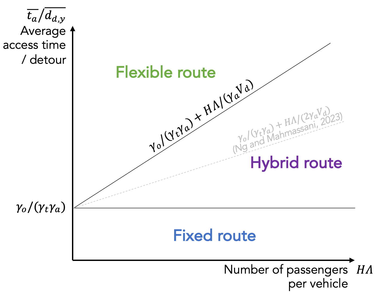
Figure 2: Illustration of Demarcation of Fixed, Hybrid, and Flexible Route from Result 1 (Ignoring Additional Vehicle Requirement)

This also delineates the hybrid route case where the access cost saving is greater than the operational cost but not enough to cover the extra riding cost for all passengers. Compared to the previous results by Ng and Mahmassani (2023) (shown by the grey dashes), Result 1 demarcates the previous marginal cases between fixed and flexible routes where the hybrid route would provide better services. Eq. 11 effectively means the first $F(x_{f}^{*})$ passengers should be served with a flexible route, regardless of the specific x-directional demand distribution. The number increases with the vehicle speed $V_{d}$, access cost $\gamma_{a}\overline{t_{a}}$ (walking time), and value of time $\gamma_{t}$, and decreases with the headway $H$, mean detour $\overline{d_{d,y}}$, operating cost $\gamma_{o}$, and vehicle cost $\gamma_{v}$. This aligns with the trade-offs of savings in access cost with extra riding time and operational costs incurred by detours.

The vehicle cost $\gamma_{v}$ suggests extra vehicles needed for the detours in flexible routes would elevate the cost and limit the extent of the flexible route at optimum. Determining the optimal fleet size conditioned on the optimal flexible portion leads to Result 2, where $s^{*}$ increases naturally with factors that lead to longer flexible route portions.

Result 2.

For a hybrid route (with a fixed headway $H$), the optimal fleet size $s^{*}$ can be expressed in Eq. 15, which is independent of the x-directional demand distribution $f(x)$.

$$s^{*} =\frac{2}{H}\left(\frac{L_{x}}{V_{d}}+\gamma_{a}\overline{t_{a}}-\frac{\gamma_{o}}{\gamma_{t}}\overline{d_{d,y}}-2\frac{\gamma_{v}}{\gamma_{t}}\frac{\overline{d_{d,y}}}{V_{d}}+T_{l}\right)$$ (15)

Proof.

Eq. 15 can be obtained by combining Eq. 3.1.1 and 11. ∎

3.1.2 Uniform Demand Distribution.

We now show specific examples of x-directional demand distribution. Assuming that the demand density follows a uniform distribution with density $\lambda$, i.e., $f(x)=\lambda$, we get $F(x)=\lambda x$ and $\Lambda=\lambda L_{x}$. $c(x_{f})$ in Eq. 10 is then simplified in Eq. 16.

$$c(x_{f}) =\gamma_{t}\gamma_{a}\overline{t_{a}}\lambda(L_{x}-x_{f})+\gamma_{t}\gamma_{w}\lambda L_{x}\frac{H}{2}$$

$$\quad+\gamma_{t}\frac{\lambda L_{x}^{2}}{2V_{d}}+\gamma_{t}\frac{\lambda^{2}}{2}H\frac{\overline{d_{d,y}}}{V_{d}}x_{f}^{2}$$

$$\quad+\gamma_{o}\frac{L_{x}}{H}+\gamma_{o}\lambda\overline{d_{d,y}}x_{f}$$

$$\quad+\gamma_{v}\frac{2}{H}\left(\frac{L_{x}}{V_{d}}+\frac{H\overline{d_{d,y}}}{V_{d}}\lambda x_{f}+T_{l}\right)$$ (16)

The optimal flexible route portion under a uniform distribution $x_{f,uni}^{*}$ in Eq. 17 is then obtained by solving Eq. 11 with $F(x_{f,uni}^{*})=\lambda x_{f,uni}^{*}$.

$$x_{f,uni}^{*} =\frac{V_{d}}{\lambda H}\left(\gamma_{a}\frac{\overline{t_{a}}}{\overline{d_{d,y}}}-\frac{\gamma_{o}}{\gamma_{t}}-2\frac{\gamma_{v}}{\gamma_{t}}\frac{1}{V_{d}}\right)$$ (17)

3.1.3 Triangular Demand Distribution.

We may also assume a more likely scenario — increasing demand density closer to the transit station or downtown (see Figure 1). For a triangular distribution with demand density $f(x)$ starting with $0$ and increasing linearly with $x$ to $\lambda_{0}$ at the end, $f(x)=\lambda_{0}/L_{x}\cdot x$, $F(x)=\lambda_{0}/2L_{x}\cdot x^{2}$, and $\Lambda=\lambda_{0}L_{x}/2$. The total cost function $c(x_{f})$ and the optimal flexible route portion under a triangular distribution $x_{f,tri}^{*}$ can be obtained similarly in Eq. 18 and 19.

$$c(x_{f}) =\gamma_{t}\gamma_{a}\overline{t_{a}}\frac{\lambda_{0}}{2}\left(L_{x}-\frac{x_{f}^{2}}{L_{x}}\right)$$

$$\quad+\gamma_{t}\gamma_{w}\frac{\lambda_{0}L_{x}}{2}\frac{H}{2}+\gamma_{t}\frac{\lambda_{0}L_{x}^{2}}{6V_{d}}+\gamma_{t}H\frac{\overline{d_{d,y}}}{V_{d}}\lambda_{0}^{2}\frac{x_{f}^{4}}{8L_{x}^{2}}$$

$$\quad+\gamma_{o}\frac{L_{x}}{H}+\gamma_{o}\overline{d_{d,y}}\frac{\lambda_{0}x_{f}^{2}}{2L_{x}}$$

$$\quad+\gamma_{v}\frac{2}{H}\left(\frac{L_{x}}{V_{d}}+\frac{H\overline{d_{d,y}}}{V_{d}}\frac{\lambda_{0}x_{f}^{2}}{2L_{x}}+T_{l}\right)$$ (18)

$$x_{f,tri}^{*} =\sqrt{\frac{2L_{x}V_{d}}{\lambda_{0}H}\left(\gamma_{a}\frac{\overline{t_{a}}}{\overline{d_{d,y}}}-\frac{\gamma_{o}}{\gamma_{t}}-2\frac{\gamma_{v}}{\gamma_{t}}\frac{1}{V_{d}}\right)}$$ (19)

The comparison of the results under the two demand distributions leads to Result 3.

Result 3.

For a hybrid route assuming the same total demand $\Lambda$, the optimal flexible portion under a triangular distribution $x_{f,tri}^{*}$ is always longer than that under a uniform distribution $x_{f,uni}^{*}$. Specifically, $x_{f,tri}^{*}=\sqrt{L_{x}x_{f,uni}^{*}}$.

Proof.

$x_{f,tri}^{*}=\sqrt{L_{x}x_{f,uni}^{*}}$ is obtained by combining Eq. 11 and Eq. 19. Then, $x_{f,tri}^{*}>x_{f,uni}^{*}$ for $x_{f,uni}^{*}<L_{x}$. ∎

3.2 Joint Optimization of the Flexible Route Portion, Fleet Size, and Headway with Variable Vehicle Sizes

How would the deployment of CAVs of different vehicle sizes affect the flexible route portion, fleet size, and headway in semi-on-demand routes? We examine this problem by considering the required fleet size and respective operating cost $\gamma_{o}(b)$ and vehicle cost $\gamma_{v}(b)$ of each vehicle size $b\in\mathcal{B}$ (in pax/veh), where $\mathcal{B}$ is a set of vehicle sizes. We also relax the assumption of a fixed headway $H$ to allow a variable headway function $h(x_{f},s)$. A trade-off is expected between vehicle cost (larger vehicles and less frequent services) and waiting time (longer headway).

The fleet size $s$ in Eq. 3.1.1 is rewritten with the headway function $h(x_{f},s)$ in Eq. 20. After re-arranging the terms, we obtain Eq. 21.

$$s =\frac{2}{h(x_{f},s)}\left(\frac{L_{x}}{V_{d}}+\frac{\overline{d_{d,y}}}{V_{d}}F(x_{f})h(x_{f},s)+T_{l}\right)$$ (20)

$$h(x_{f},s) =\frac{L_{x}+T_{l}V_{d}}{sV_{d}/2-\overline{d_{d,y}}F(x_{f})}$$ (21)

We also need to update several cost components for the variable headway. Firstly, the waiting cost depends on the headway function in Eq. 22. Next, riding costs for y-directional detours also vary with the headway in Eq. 23, as fewer passengers in each vehicle mean fewer detours in the flexible portion.

$$c_{w}(x_{f},s) =\gamma_{t}\gamma_{w}\Lambda\frac{h(x_{f},s)}{2}$$ (22)

$$c_{t,y}(x_{f},s) =\gamma_{t}\frac{\overline{d_{d,y}}}{2V_{d}}F(x_{f})^{2}h(x_{f},s)$$ (23)

For operating costs, the x-component of operating costs depends on $h(x_{f},s)$ in Eq. 24 because of the service frequency change. However, the y-component is unaffected due to the constant number of detours per hour. Lastly, the vehicle cost can no longer be simply expressed as a function of $x_{f}$ as in Eq. 9, but is still directly proportional to the fleet size in Eq. 25.

$$c_{o,x}(x_{f},s) =\gamma_{o}(b)\frac{L_{x}}{h(x_{f},s)}$$ (24)

$$c_{v}(s) =\gamma_{v}(b)s$$ (25)

As vehicle sizes and corresponding costs are discrete, it provides an opportunity to enumerate $b$ and solve for the optimal $x_{f}$ and $s$ that minimize total costs. We impose a capacity requirement constraint that the provided hourly capacity $b/h(x_{f},s)$ has to be greater than the demand $\Lambda$ by a buffer of $\rho$ (to avoid over-capacity due to demand variations), i.e., $\rho b/h(x_{f},s)\geq\Lambda$. Combined with Eq. 21, this results in a lower bound of the fleet size $s$ for each vehicle capacity $b$ in Eq. 26.

$$s\geq\frac{2}{V_{d}}\left(\frac{\Lambda}{\rho b}(L_{x}+T_{l}V_{d})+\overline{d_{d,y}}F(x_{f})\right)$$ (26)

We can formulate a mathematical problem (Eq. 3.2) to minimize the total cost $c(x_{f},s,b)$ with respect to $x_{f}$, $s$, and $b$, subject to the capacity requirement constraint in Eq. 26. The analytical expression of optimal $x_{f}$ and $s$ is complicated, so it is more practical to solve the minimization numerically. For each discrete $b$, we can solve for $(x_{f}^{*},s^{*})$ that minimize $c(x_{f},s,b)$ and subsequently apply Eq. 21 to obtain the optimal headway $h(x_{f}^{*},s^{*})$. We note that Result 1 still applies here for a determined headway, which is useful for conducting analysis but not obtaining a solution.

$$\min_{x_{f},s,b}c(x_{f},s,b)$$

$$=\gamma_{t}\gamma_{a}\overline{t_{a}}(\Lambda-F(x_{f}))+\gamma_{t}\gamma_{w}\Lambda\frac{h(x_{f},s)}{2}$$

$$\quad+\gamma_{t}\frac{1}{V_{d}}\int_{0}^{L_{x}}F(x)dx+\gamma_{t}h(x_{f},s)\frac{\overline{d_{d,y}}}{2V_{d}}F(x_{f})^{2}$$

$$\quad+\gamma_{o}(b)\frac{L_{x}}{h(x_{f},s)}+\gamma_{o}(b)\overline{d_{d,y}}F(x_{f})$$

$$\quad+\gamma_{v}(b)\frac{2}{h(x_{f},s)}\left(\frac{L_{x}}{V_{d}}+\frac{h(x_{f},s)\overline{d_{d,y}}}{V_{d}}F(x_{f})+T_{l}\right)$$

$$\text{subject to}~{}~{}~{}~{}~{}\text{Eq.}~{}(\ref{eq:s_LB}),~{}~{}~{}0\leq x_{f}\leq L_{x},~{}~{}~{}b\in\mathcal{B}$$ (27)

4 Numerical Examples

To demonstrate the mathematical models and benefits of the semi-on-demand routes, we present two sets of numerical examples, each with two Chicago bus routes illustrated in Figure 3 (also studied by Ng and Mahmassani (2023)). The first example is the joint optimization of the flexible route portion $x_{f}$ and fleet size $s$ with a given headway $H$ (Section 3.1), and the second is the joint optimization of flexible route portion $x_{f}$, fleet size $s$, headway $H$, and vehicle size $b$ (Section 3.2). The two Chicago Transit Authority (CTA) bus routes studied, CTA126 and CTA84, mainly connect passengers to downtown and a railway station respectively.

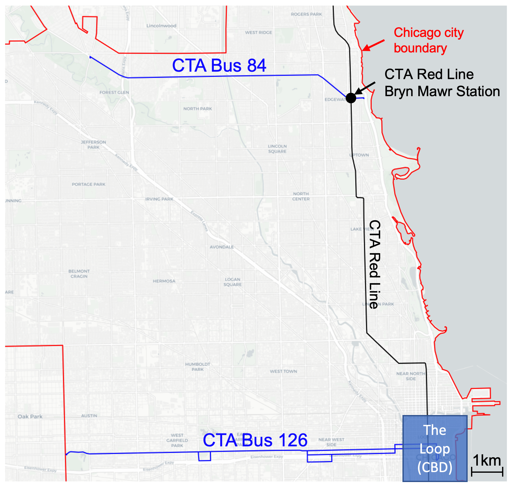
Figure 3: Maps of Bus Routes CTA126 and CTA84 in Chicago (Chicago Transit Authority 2022a, b)

The scenario details and parameters follow Ng and Mahmassani (2023): a demand profile with $\Lambda=80$ pax/h is used with a 15-min headway $H$ and x-directional demand distributions as uniform and triangular distributions previously discussed in Section 3. The other parameters are as follows: the value of time $\gamma_{t}$ is $16.5/h, cost factors of access(walking) $\gamma_{a}$ and waiting $\gamma_{w}$ are 2 and 1.5; the distance-based operational cost $\gamma_{o}$ is $0.5/km and vehicle time cost $\gamma_{v}$ is $12/h for a minibus (Tirachini and Antoniou 2020); the vehicle speed $V_{d}$ is 30km/h and layover time $T_{l}$ is 10min; the route length $L_{x}$ is 10.9km and 13.4km for CTA126 and CTA84 respectively; with the assumption of a uniform distribution of y-directional demand in the catchment areas, the average access time $\overline{t_{a}}$ is 2.25min for CTA126 and 6.75min for CTA84 and mean detour $\overline{d_{d,y}}$ is 0.13km and 0.53km respectively.

4.1 Joint Optimization of the Flexible Route Portion and Fleet Size given a Headway

The costs and optimal flexible route portion $x_{f}^{*}$ are obtained with the analytical formula in Eq. 16-19 with the aforementioned parameters.

Under uniform distribution of demand in the x-direction, Figure 4 shows the total cost, fleet size, and average cost component of the case CTA126, respectively. The optimal flexible route portion $x_{f,uni}^{*}=7.91$km serves $F(x_{f}^{*})=62$pax with the optimal fleet size $s^{*}=4.76$. When the flexible route portion increases, access cost decreases linearly, while riding cost increases quadratically. As the mean deviation $\overline{d_{d,y}}$ in this case is relatively small, the effect of flexible portions on operating and vehicle costs is minimal, favoring a longer flexible route. Besides, we note that for fixed route operation, the fleet size $s(0)=4.24$, which if not shared across routes would also require 5veh, the same as the hybrid route service. This suggests that the simplified result subject to a fixed fleet size by setting $\gamma_{v}=0$ suffices given the limited detours required.

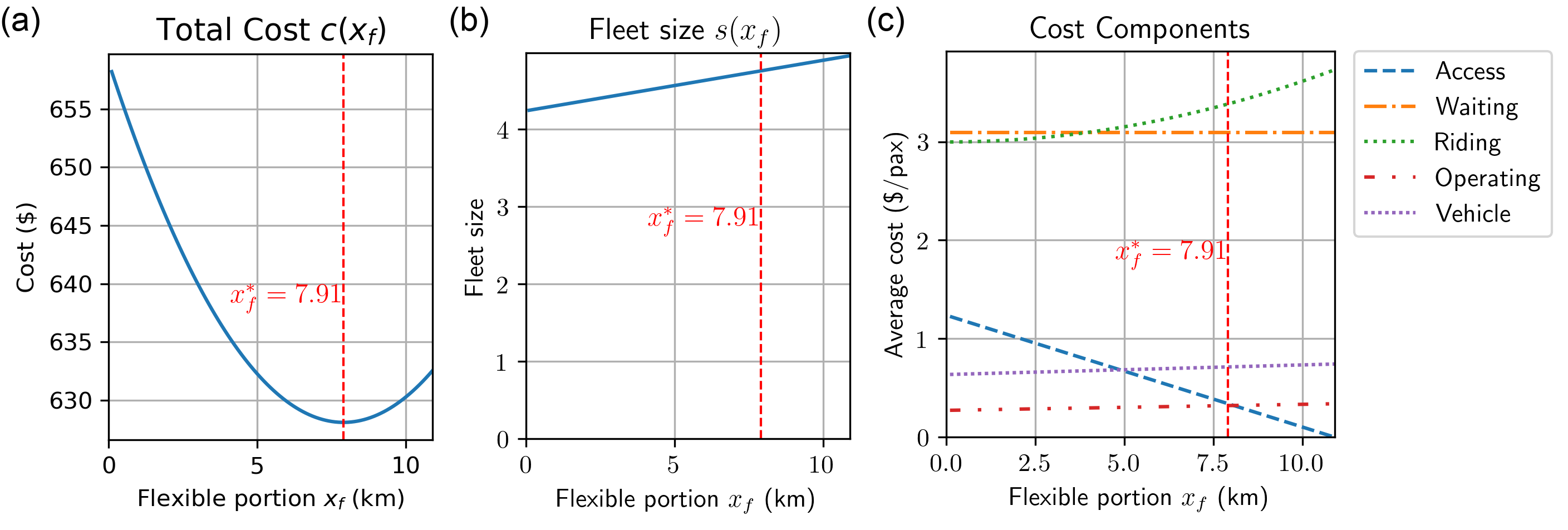
Figure 4: Total Costs $c(x_{f})$ (a), Fleet Size $s(x_{f})$ (b), and Average Cost Components (c) of Case CTA126 with respect to Flexible Route Portion $x_{f}$ under Uniform Demand Distribution

The results of triangular distribution in Figure 5 favor flexible routes even more with $x_{f,tri}^{*}=9.28$km. As previously discussed, this is equal to $\sqrt{L_{x}x_{f,uni}^{*}}$, or 12.6% of the route length longer. The concentrated demand closer to the train station favors a longer flexible route portion. On the other hand, access and riding costs change more rapidly closer to the end as shown in Figure 5(c).

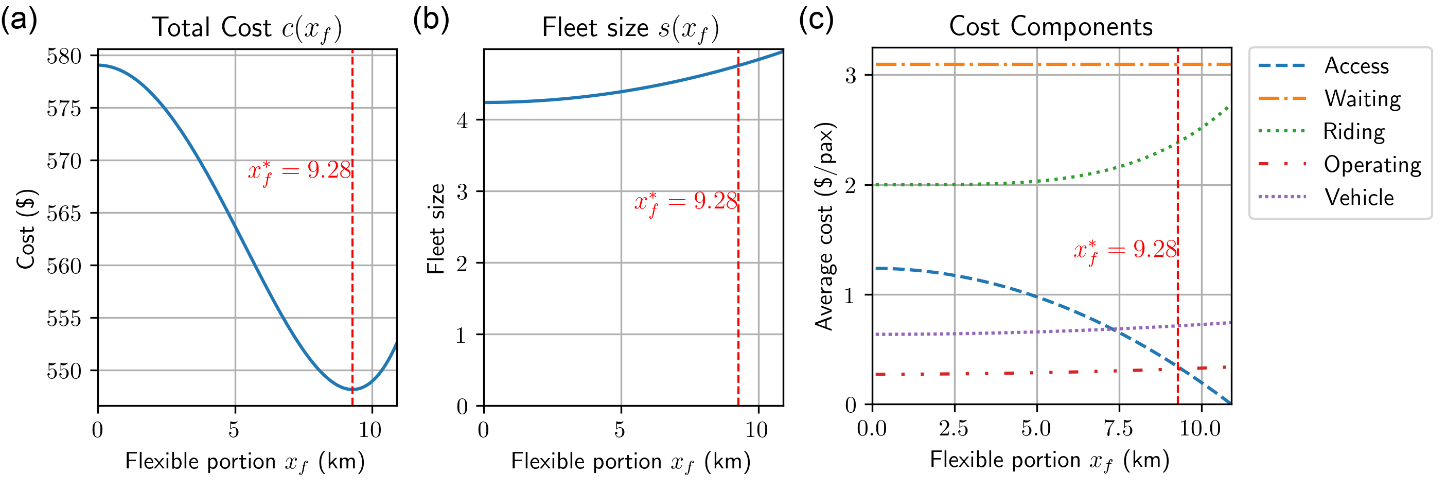
Figure 5: Total Costs $c(x_{f})$ (a), Fleet Size $s(x_{f})$ (b), and Average Cost Components (c) of Case CTA126 with respect to Flexible Route Portion $x_{f}$ under Triangular Demand Distribution

Figure 6 shows similar results for the case CTA84 under a uniform demand distribution. The mean detour $\overline{d_{d,y}}$ and average access time $\overline{t_{a}}$ are greater than those in the last case, implying higher potential savings in access cost but more vehicle detours for the flexible route portion. The optimal flexible portion $x_{f,uni}^{*}$ is 6.90km, serving $F(x_{f}^{*})=45$pax with the optimal fleet size $s^{*}=6.37$. The smaller flexible portion is explained by the faster increases in riding, operating, and vehicle costs.

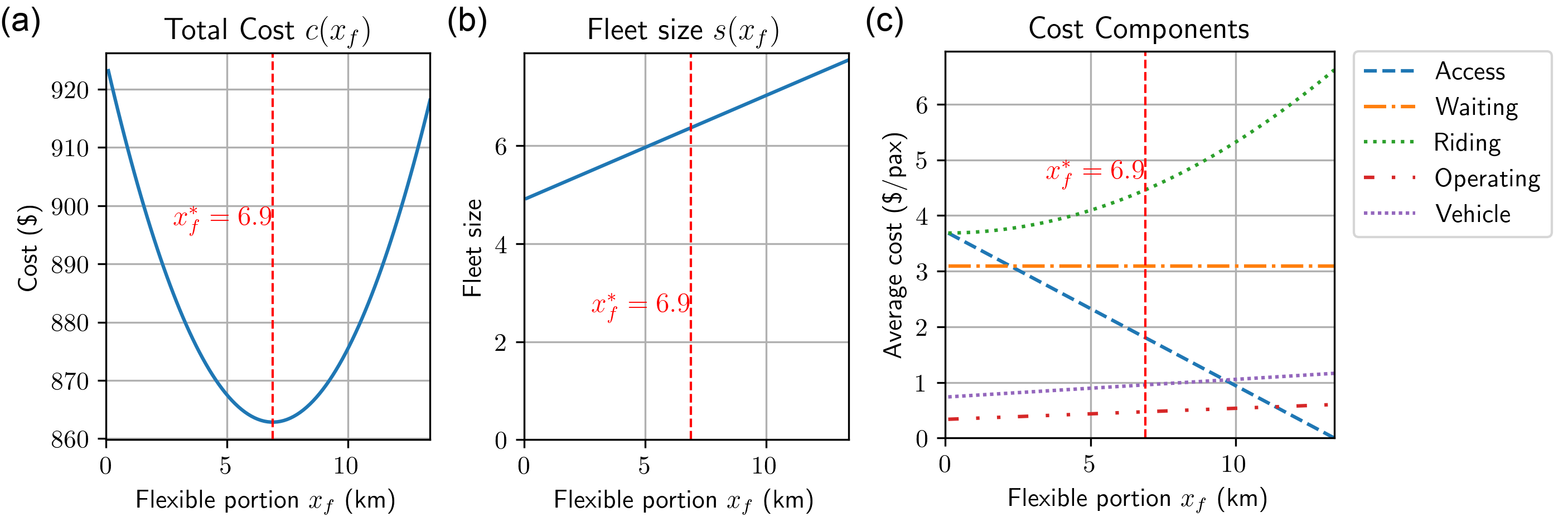
Figure 6: Total Costs $c(x_{f})$ (a), Fleet Size $s(x_{f})$ (b), and Average Cost Components (c) of Case CTA84 with respect to Flexible Route Portion $x_{f}$ under Uniform Demand Distributions

The case of a triangular distribution in demand is illustrated in Figure 7. While the optimal flexible portion is extended to $x_{f,tri}^{*}=9.61km$, the flexible route proportion over the route length is still smaller than CTA126 (CTA84 is a longer route).

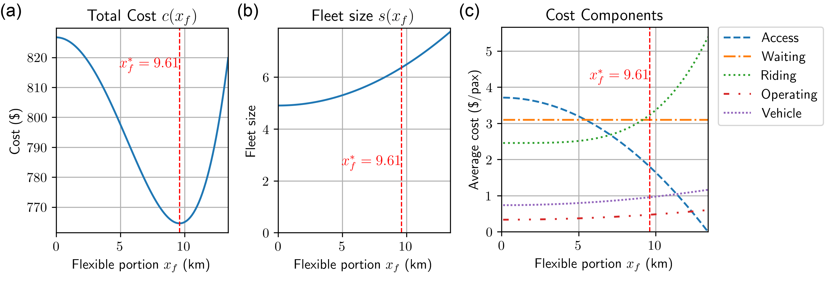
Figure 7: Total Costs $c(x_{f})$ (a), Fleet Size $s(x_{f})$ (b), and Average Cost Components (c) of Case CTA84 with respect to Flexible Route Portion $x_{f}$ under Triangular Demand Distributions

In summary, serving passengers further away with a flexible route portion lowers the total cost, in particular user cost, for both routes. Smaller mean detour $\overline{d_{d,y}}$ and an increasing demand gradient favor longer flexible portions.

4.2 Joint Optimization of the Flexible Route Portion, Fleet Size, and Headway with Variable Vehicle Sizes

The total cost minimization in Eq. 3.2 can be achieved by solving for the optimal $x_{f}$ and $s$ with numerical solvers (L-BFGS-B in this example) for each vehicle size $b$. This subsection shows results under uniform distribution of demand.

Vehicle operating costs $\gamma_{o}$, which are distance-based, and time-based capital costs $\gamma_{v}$ are derived from different vehicle classes and capacities as per Tirachini and Antoniou (2020) (under their scenario of 50% reduction in driving costs). The vehicle types considered are car, van, 20-seater, minibus, and bus, with capacities $b\in$[5,8,20,44,70] (pax/veh), operating costs $\gamma_{o}\in$ [0.6187, 0.6370, 0.6938, 0.7507, 0.8900] ($/km) and vehicle costs $\gamma_{v}\in$ [2.53, 3.63, 7.59, 11.55, 15.73] ($/h). The capacity buffer is set as $\rho=0.7$.

Figure 8(a) shows the total costs $c(x_{f},s^{*},b)$ under the optimal fleet size for the CTA126 case. It illustrates the impact of varying the flexible route portion $x_{f}$ while optimizing the fleet size. For all vehicle types, the cost curve is monotonically decreasing, indicating only flexible route services. Figure 8(b) shows the optimal fleet sizes $s^{*}$ under varying flexible route portions $x_{f}$. To ensure sufficient capacity to meet the demand, the fleet sizes for cars and vans are the minimum required independent of $x_{f}$. For other vehicle types, the optimal fleet sizes increase gradually to serve more detours. The headways shown in Figure 8(c) are much lower than the 15-minute headway setting in the previous examples, suggesting that the reduction in waiting time outweighs the increase in operating cost (Figure 8(d)), if the capital and operating costs of SAVs are as low as forecasted (relative to the assumed values of time).

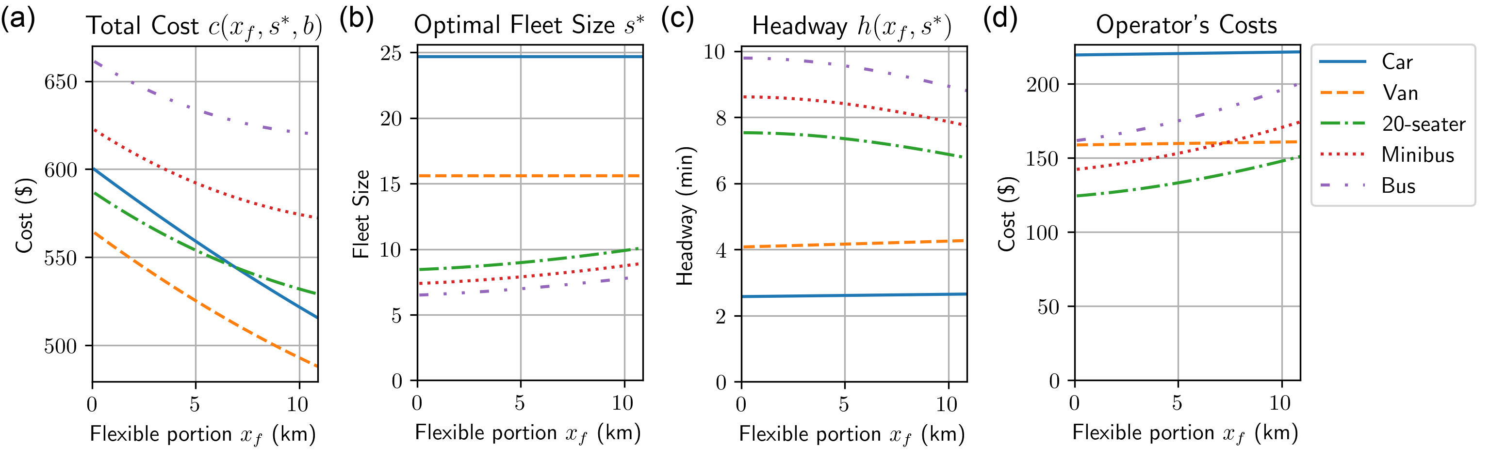
Figure 8: Total Costs under Optimal Fleet Size $c(x_{f},s^{*},b)$ (a), Optimal Fleet Size $s^{*}$ (b), Headway $h(x_{f},s^{*})$ (c), and Total Operator Costs (d) with respect to Flexible Route Portion $x_{f}$ in Cases CTA126

Figure 9 shows similar results for the case CTA84. The changes with increasing flexible route portions are more considerable due to the larger detours for each passenger.

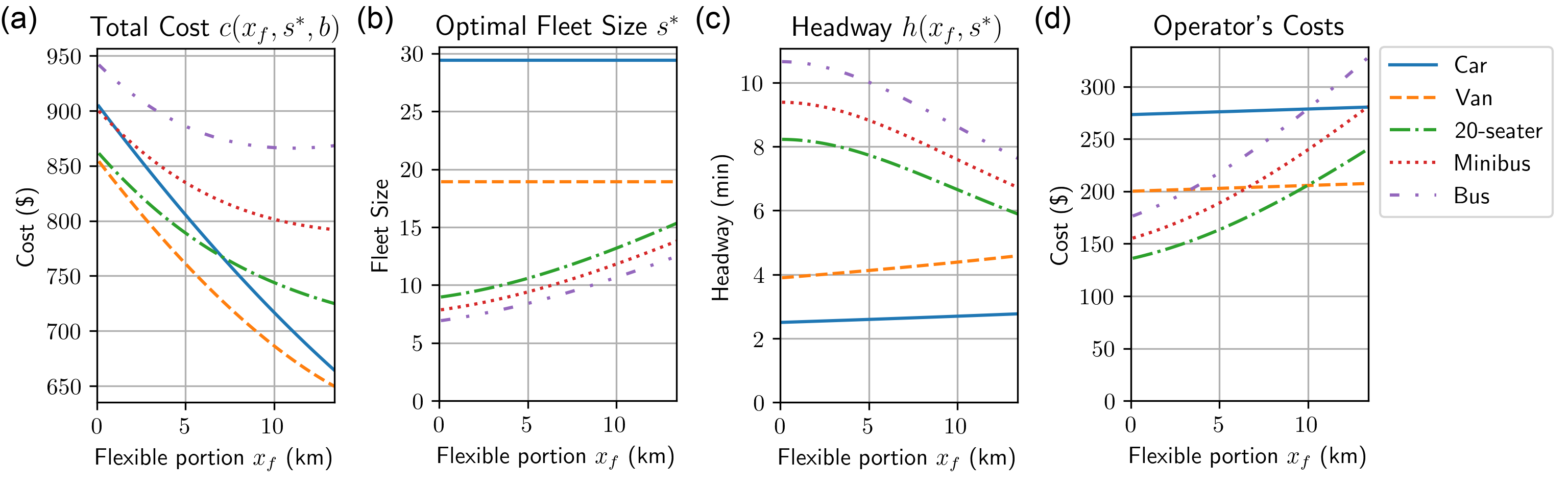
Figure 9: Total Costs under Optimal Fleet Size $c(x_{f},s^{*},b)$ (a), Optimal Fleet Size $s^{*}$ (b), Headway $h(x_{f},s^{*})$ (c), and Total Operator Costs (d) with respect to Flexible Route Portion $x_{f}$ in Cases CTA84

Flexible routes are optimal in most cases, different from the previous results in Section 4.1 where hybrid routes are optimal under a constant 15-minute headway. This is primarily contributed by the much lower headway, particularly for smaller vehicle sizes. However, the operator costs required to provide such low headway are considerably higher than the current human-driven fixed route operations ($124 and $150 for CTA126 and CTA84 respectively). If a budget constraint is applied, the optimal results would likely be hybrid route similar to Section 4.1 where changes in operator costs are much smaller under fixed headway.

Table 2 lists the detailed results.

Table 2: Results of Joint Optimization of Vehicle Size, Flexible Route Portion, and Fleet Size

Bus route				CTA126					CTA84
Vehicle	Type			Car	Van	20- Seater	Mini- bus	Stand- ard bus	Car	Van	20- Seater	Mini- bus	Stand- ard bus
	Size	b	pax /veh	5	8	20	44	70	5	8	20	44	70
Optimal variable	Flexible portion	$x_{f}^{*}$	km	10.90	10.90	10.90	10.90	10.90	13.40	13.40	13.40	13.40	11.04
	Fleet size	$s^{*}$	veh	24.69	15.60	10.10	8.92	7.93	29.42	18.90	15.33	13.79	11.20
	Headway	$h^{*}$	min	2.65	4.27	6.77	7.75	8.81	2.77	4.58	5.89	6.72	8.31
Average time	Access	$\overline{t_{a}}$	min	0.00	0.00	0.00	0.00	0.00	0.00	0.00	0.00	0.00	1.19
	Waiting	$\overline{t_{w}}$	min	1.33	2.14	3.39	3.87	4.40	1.38	2.29	2.95	3.36	4.16
	Riding	$\overline{t_{t}}$	min	11.37	11.66	12.10	12.28	12.47	15.37	16.66	17.59	18.18	17.41
Time std. dev.	Access	$\sigma_{t,a}$	min	0.00	0.00	0.00	0.00	0.00	0.00	0.00	0.00	0.00	1.45
	Waiting	$\sigma_{t,w}$	min	0.77	1.23	1.96	2.24	2.54	0.80	1.32	1.70	1.94	2.40
	Riding	$\sigma_{t,r}$	min	6.75	6.93	7.20	7.30	7.41	9.63	10.42	10.98	11.33	11.04
Cost	Access	$c_{a}$	$	0.00	0.00	0.00	0.00	0.00	0.00	0.00	0.00	0.00	52.24
	Waiting	$c_{w}$	$	43.76	70.48	111.76	127.85	145.29	45.70	75.64	97.24	110.96	137.12
	Riding (x-dir.)	$c_{t,x}$	$	239.80	239.80	239.80	239.80	239.80	294.80	294.80	294.80	294.80	294.80
	Riding (y-dir.)	$c_{t,y}$	$	10.37	16.71	26.49	30.31	34.44	43.33	71.72	92.20	105.20	88.30
	Operational (x-dir.)	$c_{o,x}$	$	152.56	97.53	66.99	63.36	66.10	179.61	111.72	94.65	89.75	86.11
	Operational (y-dir.)	$c_{o,y}$	$	6.60	6.79	7.40	8.01	9.49	26.40	27.18	29.60	32.03	31.29
	Vehicle	$c_{v}$	$	62.47	56.63	76.66	103.01	124.80	74.43	68.61	116.38	159.26	176.19
	Total	$c$	$	515.56	487.94	529.11	572.34	619.93	664.27	649.66	724.87	792.01	866.04

4.2.1 Sensitivity to Operator Cost.

To assess the sensitivity to the forecasted operator costs (or user value of time), Figures 10 and 11 present the results under 200% and 300% of operator costs (or effectively 50% and 33% of user value of time) for case CTA84. We can see a reduction in the flexible route portion in subplots (a), where minibus hybrid route dominates in the 300% case. Additionally, the optimal flexible route portion (the cost minimum point) decreases with increasing vehicle sizes. This means smaller vehicles support the deployment of longer flexible routes with each trip serving fewer passengers and making fewer detours, whereas larger vehicles may lead to excessive cumulative detours. Although more smaller vehicles are required to serve the same demand, each trip involves smaller detours in the flexible route portion alongside shorter waiting times. This also explains the general reduction in headway with an increase in the flexible route portion in subplots (c). These findings align with Result 1, where lower operational costs ($\gamma_{o}$ and $\gamma_{v}$) and smaller headway ($H$) favor flexible routes.

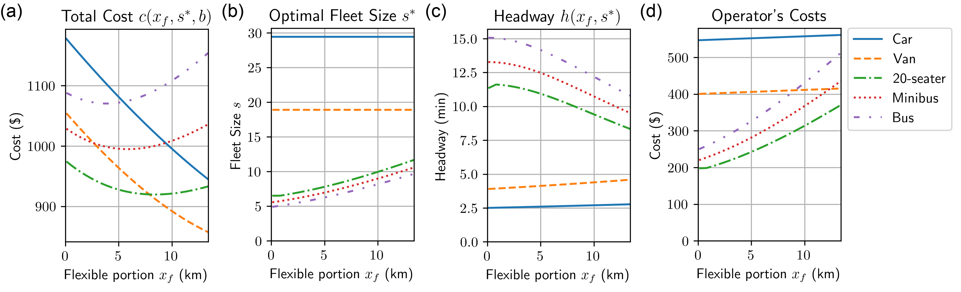
Figure 10: Total Costs under Optimal Fleet Size $c(x_{f},s^{*},b)$ (a), Optimal Fleet Size $s^{*}$ (b), Headway $h(x_{f},s^{*})$ (c), and Total Operator Costs (d) with respect to Flexible Route Portion $x_{f}$ under 200% Operator Costs for Case CTA84

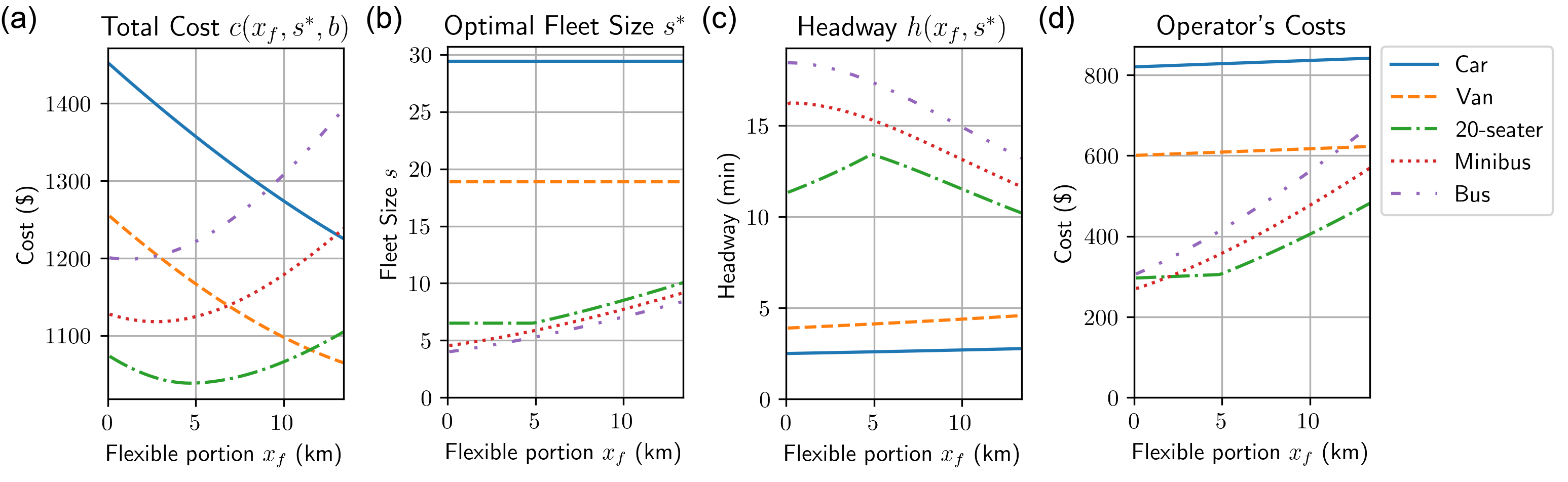
Figure 11: Total Costs under Optimal Fleet Size $c(x_{f},s^{*},b)$ (a), Optimal Fleet Size $s^{*}$ (b), Headway $h(x_{f},s^{*})$ (c), and Total Operator Costs (d) with respect to Flexible Route Portion $x_{f}$ under 300% Operator Costs for Case CTA84

In short, a balance across vehicle size is important — using 4-passenger cars would necessitate a lot of vehicles to serve the demand; utilizing larger buses could result in excessive detours and longer waiting times. The optimal scenario with the assumed operator costs in both cases is using a van of 8 passengers with only flexible route service. However, before the technology matures for the cost to fall, bigger vehicles running hybrid routes may be the optimal solution. This also applies to cases where operators face a strict budget such that the system-optimally low headway is infeasible.

Table 3 shows the detailed results.

Table 3: Results of Sensitivity Analysis for the Joint Optimization of Vehicle Size, Flexible Route Portion, and Fleet Size

Bus route CTA84				200% Operator Cost					300% Operator Cost
Vehicle	Type			Car	Van	20- Seater	Mini- bus	Stand- ard bus	Car	Van	20- Seater	Mini- bus	Stand- ard bus
	Size	b	pax /veh	5	8	20	44	70	5	8	20	44	70
Optimal variable	Flexible portion	$x_{f}^{*}$	km	13.40	13.40	8.39	5.87	3.89	13.40	13.40	4.69	2.75	1.14
	Fleet size	$s^{*}$	veh	29.42	18.90	9.19	7.27	5.90	29.42	18.90	6.51	5.20	4.24
	Headway	$h^{*}$	min	2.77	4.58	9.93	12.21	14.50	2.77	4.58	13.35	15.94	18.39
Average time	Access	$\overline{t_{a}}$	min	0.00	0.00	2.52	3.80	4.79	0.00	0.00	4.39	5.37	6.18
	Waiting	$\overline{t_{w}}$	min	1.38	2.29	4.97	6.11	7.25	1.38	2.29	6.67	7.97	9.20
	Riding	$\overline{t_{t}}$	min	15.37	16.66	16.17	15.06	14.27	15.37	16.66	14.56	13.88	13.49
Time std. dev.	Access	$\sigma_{t,a}$	min	0.00	0.00	2.12	2.60	2.92	0.00	0.00	2.79	3.09	3.31
	Waiting	$\sigma_{t,w}$	min	0.80	1.32	2.87	3.52	4.19	0.80	1.32	3.85	4.60	5.31
	Riding	$\sigma_{t,r}$	min	9.63	10.42	10.41	9.73	9.10	9.63	10.42	9.35	8.69	8.13
Cost	Access	$c_{a}$	$	0.00	0.00	111.00	167.00	210.88	0.00	0.00	193.08	236.06	271.79
	Waiting	$c_{w}$	$	45.70	75.64	163.88	201.48	239.28	45.70	75.64	220.21	263.05	303.48
	Riding (x-dir.)	$c_{t,x}$	$	294.80	294.80	294.80	294.80	294.80	294.80	294.80	294.80	294.80	294.80
	Riding (y-dir.)	$c_{t,y}$	$	43.33	71.72	60.94	36.60	19.07	43.33	71.72	25.56	10.50	2.07
	Operational (x-dir.)	$c_{o,x}$	$	359.23	223.44	112.33	98.85	98.69	538.84	335.17	125.39	113.58	116.71
	Operational (y-dir.)	$c_{o,y}$	$	52.80	54.36	37.08	28.04	22.02	79.19	81.54	31.07	19.72	9.67
	Vehicle	$c_{v}$	$	148.87	137.21	139.53	167.99	185.61	223.30	205.82	148.23	180.19	200.23
	Total	$c$	$	944.71	649.66	919.55	994.77	1070.36	1225.16	1064.68	1038.35	1117.89	1198.76

5 Case Study

To investigate the applicability of the described semi-on-demand hybrid routes in transit feeders, this case study makes use of a real-world transit network and demand data in the Chicago metropolitan area. We classify analytically areas served by feeder routes to each railway station into fixed route and flexible route service areas with analytical formula in Section 3.1.

Demand data are adapted from the activity-based demand model CT-RAMP from Chicago Metropolitan Agency for Planning (Parsons Brinckerhoff 2011), where trips originate and end at micro analysis zones (MAZs). Only trips that are assigned to trains and originate outside walking distance are included, which equates to approximately 78,000 hourly trips after aggregation into three peak hours daily. The existing train stations of the commuter rail, Metra, (City of Chicago 2012) and rapid transit system, Chicago “L”, (Chicago Transit Authority 2022b) are imported into the Geographic Information System (GIS) model.

The geospatial pre-processing is as follows. Voronoi zones are created around each station to assign MAZs to their closest stations. The x-axis in the previous model is set between the station and the furthest MAZ in each Voronoi zone. The perpendicular y-axis ($x=0$) then separates the zone into two sub-zones, each of which contains one or more parallel feeder catchments based on the maximum walking distance.

We then carry out the analysis in each sub-zone, by calculating the number of passengers to serve in flexible route portions, i.e., $F(x_{f}^{*})$ in Eq. 11. This suggests serving these passengers with flexible routes would not only reduce their travel costs, but also total costs of users and operators. Instead of a uniform or triangular distribution assumption, the analysis directly captures $f(x)$ from the number of trips in each MAZ (at its center).

The parameters are set as follows: The maximum access time is 15min and the walking speed is 4km/h, resulting in a catchment width of 2km and average detour $\overline{d_{d,y}}$ of 0.67km (assuming a uniform distribution of y-directional demand); other parameters follow the previous numerical example in Section 4.1. The optimal number of passengers in the flexible route portion $F(x_{f}^{*})$ is then 35.5 with Eq. 11, equivalent to around 9 pax/trip.

Figure 12 shows which MAZs are served with fixed routes (blue dots) and flexible routes (in green dots) in each zone (in gray boundary). The flexible route service areas are mostly found in suburbs and rural areas far from downtown, with sparser demand and bigger gaps between transit lines.

The detailed results are shown in Table 4. 787 routes (86.6% of the total) are semi-on-demand hybrid routes, serving 3,562 MAZs (62.1%) with flexible routes. However, this accounts for only 18,989pax/h (24.3%). The large coverage area accounting for a small portion of demand highlights the use case of flexible feeders for low-demand-density areas. The operator cost increases by 49.0%, arising from the additional mileage and vehicles needed. This, however, is a small portion of the total costs, based on the SAV cost forecast. Higher operating and vehicle costs would reduce $x_{f}^{*}$ and the extent of flexible routes. While hybrid routes only save 7.9% user cost and 6.0% total cost in general, they make significant differences among travelers who use the flexible route portion by eliminating the access cost, accounting for a saving of 29.8% user cost. This enhances the attractiveness of transit systems to travelers in these zones who are usually further from the train stations. (The benefits brought by mode shift to transit are however not captured in this study.)

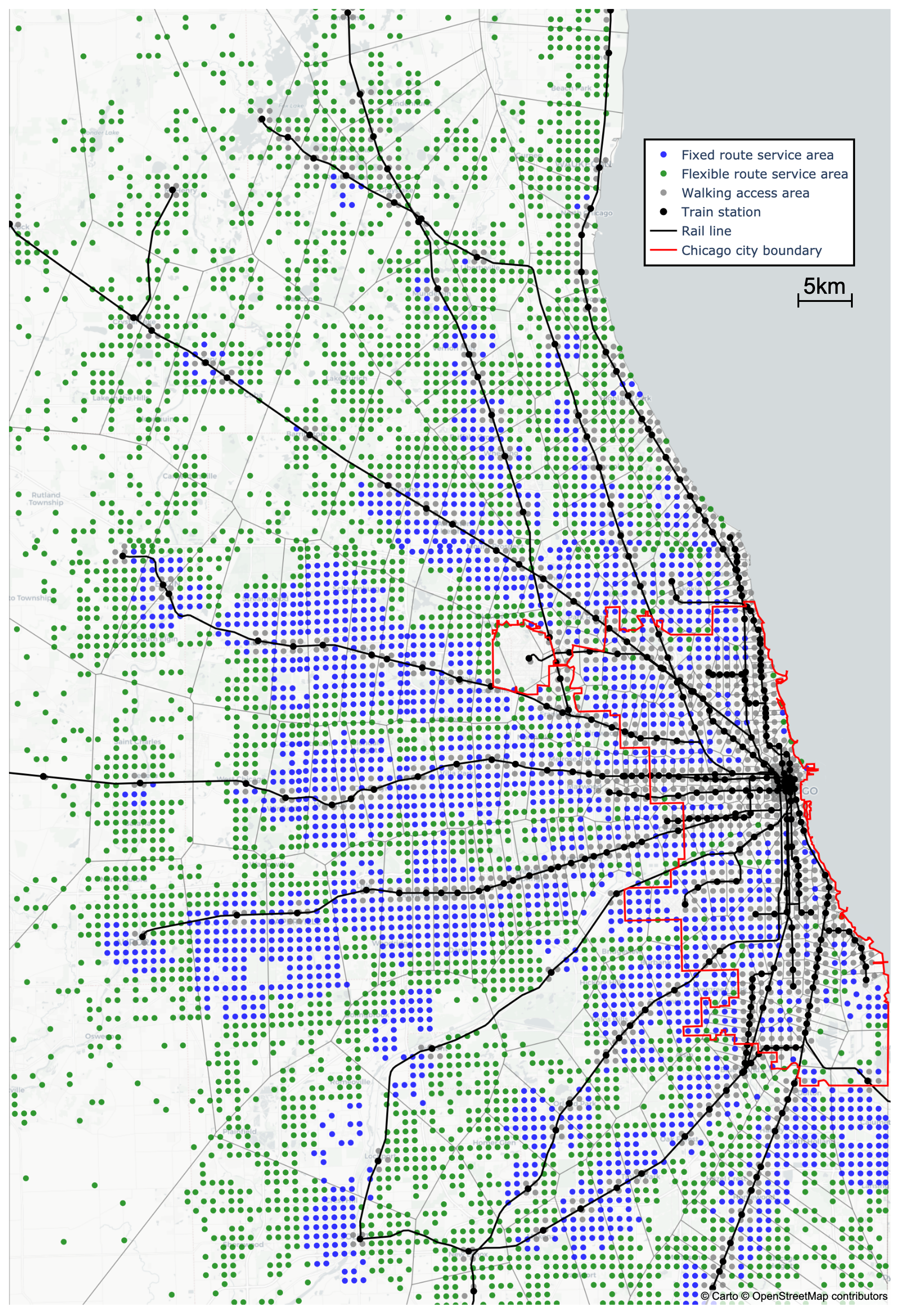
Figure 12: Case Study Results of Fixed Route and Flexible Route Service Area for Feeders to Train Stations (Chicago Transit Authority 2022b, City of Chicago 2012)

Table 4: Case Study Results of Fixed Route and Flexible Route Service Area for Feeders to Train Stations

Service area		Among all feeders			Among semi-on-demand hybrid route feeders			Among MAZs in flexible route service areas
Service mode		Fixed route	Semi-on- demand route	Percent- age change	Fixed route	Semi-on- demand route	Percent- age change	Fixed route	Semi-on- demand route	Percent- age change
Number of feeder routes		909		N/A	787		N/A	787		N/A
Number of MAZs covered		5,732		N/A	5,479		N/A	3,562		N/A
Number of passengers	pax/h	78,237		N/A	49,921		N/A	18,989		N/A
Average access time	min	7.50	5.68	-24.3%	7.50	4.65	-38.0%	7.50	0.00	-100.0%
Average waiting time	min	7.50	7.50	0.0%	7.50	7.50	0.0%	7.50	7.50	0.0%
Average riding time	min	4.95	6.12	23.6%	5.96	7.79	30.8%	7.93	12.75	60.8%
Average user cost	$	8.58	7.90	-7.9%	8.86	7.79	-12.0%	9.40	6.60	-29.8%
Average operator cost	$	0.32	0.47	45.6%	0.47	0.69	49.0%	N/A	N/A	N/A
Average generalized cost	$	8.90	8.37	-6.0%	9.32	8.49	-9.0%	N/A	N/A	N/A
Total access cost	$	322,731	244,401	-24.3%	205,924	127,594	-38.0%	78,330	0	-100.0%
Total waiting cost	$	242,048	242,048	0.0%	154,443	154,443	0.0%	58,747	58,747	0.0%
Total riding cost	$	106,449	131,619	23.6%	81,780	106,950	30.8%	41,404	66,574	60.8%
Total user cost	$	671,228	618,068	-7.9%	442,147	388,987	-12.0%	178,481	125,321	-29.8%
Total operating cost	$	9,849	16,179	64.3%	9,414	15,744	67.2%	N/A	N/A	N/A
Total vehicle cost	$	15,151	20,215	33.4%	13,827	18,891	36.6%	N/A	N/A	N/A
Total operator cost	$	25,000	36,394	45.6%	23,241	34,635	49.0%	N/A	N/A	N/A
Total generalized cost	$	696,228	654,462	-6.0%	465,388	423,622	-9.0%	N/A	N/A	N/A

6 Conclusion

6.1 Summary

This study considers semi-on-demand hybrid route service in public transit systems. It serves directional demand by first offering passengers further from a transit station/downtown with on-demand flexible route service and then continuing with a traditional fixed route. It combines the economies of scale of fixed route bus service and the accessibility and flexibility of taxi and shared autonomous mobility service (SAMS).

We develop an analytical approach to delineate the conditions in which each of the route forms (fixed, hybrid, and flexible) is optimal, with tractable cost expressions that consider the total costs of users (access, waiting, and riding) and operators (operating and vehicle) in two formulations to support strategic and tactical decisions, respectively. Closed-form expressions are derived to determine the optimal flexible route portion and fleet size for hybrid routes, and consider the optimal headway with variable vehicle sizes. Through numerical examples and a case study in the Chicago metropolitan area, we demonstrate the benefits and applications of semi-on-demand feeders.

The findings demonstrate the general applicability of hybrid routes in transit networks. Serving passengers located further away with flexible routes lowers total costs, particularly user costs in access, which could potentially attract more riders to connect with the main transit system. Besides, demand gradients favor longer flexible routes, a good fit for cities with urban sprawl. In the example of joint design of flexible route portion, headway, fleet size, and vehicle size, vans with flexible routes dominate. However, minibuses with hybrid routes still play a key role when shared autonomous vehicle (SAV) costs are still high and the operating budget is limited, or during transitions to smaller vehicles and flexible routes to introduce the on-demand service and enhance service attractiveness. Our case study identifies flexible route areas in suburbs and rural areas further from the station and with coverage gaps, helping to serve more riders.

6.2 Limitations and Future Research Directions

This study develops an analysis tool for semi-on-demand hybrid route services with tractable and closed-form solutions. The resulting analytical formulation of cost and optimal flexible route portion and fleet size can aid transit agencies in planning new routes and making vehicle investment decisions in the era of SAMS. It provides a continuous approximation alternative to computationally intensive simulation-based optimization for research in large-scale transit network design with SAMS. Inherently, it is limited by the assumptions, e.g., no backtracking or significant impacts brought by headway variance. Specifically for the joint optimization including headway, the operator budget and therefore headway may be fixed, favoring hybrid route over completely flexible services. The model also allows future refinement and investigation in the following areas.

First, it can be combined with demand- and supply-side models in the transit network design problem. Demand models to investigate mode shift towards the transit system with improved first-mile-last-mile connectivity, and its competition with driving. For the supply side, a joint transit network design model that explores the implications of transit network design with the inclusion of SAMS can utilize the analytical expression derived in this study and consider multiple routes simultaneously. While this model assumes a static demand, it can be readily applied to problems with multiple horizons and time-varying design parameters and demand. The methodology can also be generalized to other network structures by transforming the space with the x-axis as the shortest path and the y-axis as the detours.

Second, research can focus on the study and forecast of connected and automated vehicles (CAVs), including cost parameters. Our numerical example and sensitivity study illustrate the attractiveness of vehicles larger than sedans to provide hybrid route feeder services, and vehicle size matters in hybrid route design and headway-fleet size decisions. Following the analytical approach developed in this paper, more accurate cost forecasts would facilitate new service planning and deployment.

Third, research with agent-based models and actual fleet control can verify the model results at a microscopic level and assess the impacts of several assumptions and design parameters. For example, backtracking is not allowed in the model, so solving the vehicle routing problem that optimizes pick-ups/drop-offs could improve the performance of the flexible route portion. A constant headway is assumed in each case, whereas simulations that account for the effects of demand and service variances on waiting time could assess schedule adherence. Vehicle capacity buffer $\rho$ allows for stochastic demand, with room for future statistical or simulation approaches to evaluate the effects of vehicle size and demand fluctuation on boarding rejection.

7 Acknowledgments

The authors would like to thank Antonios Tsakarestos of the Technical University of Munich for the valuable comments in the initial stage of the study.

References

- Abdelwahed et al. (2023) Abdelwahed A, van den Berg PL, Brandt T, Ketter W, 2023 Balancing convenience and sustainability in public transport through dynamic transit bus networks. Transportation Research Part C: Emerging Technologies 151:104100, URL http://dx.doi.org/10.1016/j.trc.2023.104100.
- Alonso-Mora et al. (2017) Alonso-Mora J, Samaranayake S, Wallar A, Frazzoli E, Rus D, 2017 On-demand high-capacity ride-sharing via dynamic trip-vehicle assignment. Proceedings of the National Academy of Sciences 114(3):462–467, URL http://dx.doi.org/10.1073/pnas.1611675114, publisher: National Academy of Sciences Section: Physical Sciences.
- Badia and Jenelius (2021) Badia H, Jenelius E, 2021 Design and operation of feeder systems in the era of automated and electric buses. Transportation Research Part A: Policy and Practice 152:146–172, URL http://dx.doi.org/10.1016/j.tra.2021.07.015.
- Calabrò et al. (2023) Calabrò G, Araldo A, Oh S, Seshadri R, Inturri G, Ben-Akiva M, 2023 Adaptive transit design: Optimizing fixed and demand responsive multi-modal transportation via continuous approximation. Transportation Research Part A: Policy and Practice 171:103643, URL http://dx.doi.org/10.1016/j.tra.2023.103643.
- Cao and Ceder (2019) Cao Z, Ceder A, 2019 Autonomous shuttle bus service timetabling and vehicle scheduling using skip-stop tactic. Transportation Research Part C: Emerging Technologies 102:370–395, URL http://dx.doi.org/10.1016/j.trc.2019.03.018.
- Chang and Schonfeld (1991) Chang SK, Schonfeld PM, 1991 Optimization Models for Comparing Conventional and Subscription Bus Feeder Services. Transportation Science 25(4):281–298, URL http://dx.doi.org/10.1287/trsc.25.4.281, publisher: INFORMS.
- Chen and Nie (2017) Chen PW, Nie YM, 2017 Analysis of an idealized system of demand adaptive paired-line hybrid transit. Transportation Research Part B: Methodological 102:38–54, URL http://dx.doi.org/10.1016/j.trb.2017.05.004.
- Chicago Transit Authority (2022a) Chicago Transit Authority, 2022a CTA - Bus Routes - Shapefile | City of Chicago | Data Portal. URL https://data.cityofchicago.org/Transportation/CTA-Bus-Routes-Shapefile/d5bx-dr8z.
- Chicago Transit Authority (2022b) Chicago Transit Authority, 2022b CTA - ’L’ (Rail) Lines - Shapefile. URL https://data.cityofchicago.org/Transportation/CTA-L-Rail-Lines-Shapefile/53r7-y88m.
- City of Chicago (2012) City of Chicago, 2012 Metra Lines. URL https://data.cityofchicago.org/Transportation/Metra-Lines/q8wx-dznq.
- Cortina, Chiabaut, and Leclercq (2023) Cortina M, Chiabaut N, Leclercq L, 2023 Fostering synergy between transit and Autonomous Mobility-on-Demand systems: A dynamic modeling approach for the morning commute problem. Transportation Research Part A: Policy and Practice 170:103638, URL http://dx.doi.org/10.1016/j.tra.2023.103638.
- Dandl et al. (2021) Dandl F, Engelhardt R, Hyland M, Tilg G, Bogenberger K, Mahmassani HS, 2021 Regulating mobility-on-demand services: Tri-level model and Bayesian optimization solution approach. Transportation Research Part C: Emerging Technologies 125:103075, URL http://dx.doi.org/10.1016/j.trc.2021.103075.
- Errico et al. (2013) Errico F, Crainic TG, Malucelli F, Nonato M, 2013 A survey on planning semi-flexible transit systems: Methodological issues and a unifying framework. Transportation Research Part C: Emerging Technologies 36:324–338, URL http://dx.doi.org/10.1016/j.trc.2013.08.010.
- Errico et al. (2021) Errico F, Crainic TG, Malucelli F, Nonato M, 2021 The Single-Line Design Problem for Demand-Adaptive Transit Systems: A Modeling Framework and Decomposition Approach for the Stationary-Demand Case. Transportation Science 55(6):1300–1321, URL http://dx.doi.org/10.1287/trsc.2021.1062, publisher: INFORMS.
- Frei, Hyland, and Mahmassani (2017) Frei C, Hyland M, Mahmassani HS, 2017 Flexing service schedules: Assessing the potential for demand-adaptive hybrid transit via a stated preference approach. Transportation Research Part C: Emerging Technologies 76:71–89, URL http://dx.doi.org/10.1016/j.trc.2016.12.017.
- Galarza Montenegro, Sörensen, and Vansteenwegen (2021) Galarza Montenegro BD, Sörensen K, Vansteenwegen P, 2021 A large neighborhood search algorithm to optimize a demand-responsive feeder service. Transportation Research Part C: Emerging Technologies 127:103102, URL http://dx.doi.org/10.1016/j.trc.2021.103102.
- Grahn, Qian, and Hendrickson (2022) Grahn R, Qian S, Hendrickson C, 2022 Optimizing first- and last-mile public transit services leveraging transportation network companies (TNC). Transportation URL http://dx.doi.org/10.1007/s11116-022-10301-z.
- Gurumurthy, Kockelman, and Zuniga-Garcia (2020) Gurumurthy KM, Kockelman KM, Zuniga-Garcia N, 2020 First-Mile-Last-Mile Collector-Distributor System using Shared Autonomous Mobility. Transportation Research Record 2674(10):638–647, URL http://dx.doi.org/10.1177/0361198120936267, publisher: SAGE Publications Inc.
- Huang et al. (2020) Huang D, Gu Y, Wang S, Liu Z, Zhang W, 2020 A two-phase optimization model for the demand-responsive customized bus network design. Transportation Research Part C: Emerging Technologies 111:1–21, URL http://dx.doi.org/10.1016/j.trc.2019.12.004.
- Hyland and Mahmassani (2020) Hyland M, Mahmassani HS, 2020 Operational benefits and challenges of shared-ride automated mobility-on-demand services. Transportation Research Part A: Policy and Practice 134:251–270, URL http://dx.doi.org/10.1016/j.tra.2020.02.017.
- Leffler et al. (2021) Leffler D, Burghout W, Jenelius E, Cats O, 2021 Simulation of fixed versus on-demand station-based feeder operations. Transportation Research Part C: Emerging Technologies 132:103401, URL http://dx.doi.org/10.1016/j.trc.2021.103401.
- Levin et al. (2019) Levin MW, Odell M, Samarasena S, Schwartz A, 2019 A linear program for optimal integration of shared autonomous vehicles with public transit. Transportation Research Part C: Emerging Technologies 109:267–288, URL http://dx.doi.org/10.1016/j.trc.2019.10.007.
- Li, Lee, and Lo (2023) Li M, Lee E, Lo HK, 2023 Frequency-based zonal flexible bus design considering order cancellation. Transportation Research Part C: Emerging Technologies 152:104171, URL http://dx.doi.org/10.1016/j.trc.2023.104171.
- Li and Quadrifoglio (2010) Li X, Quadrifoglio L, 2010 Feeder transit services: Choosing between fixed and demand responsive policy. Transportation Research Part C: Emerging Technologies 18(5):770–780, URL http://dx.doi.org/10.1016/j.trc.2009.05.015.
- Liu, Qu, and Ma (2021) Liu X, Qu X, Ma X, 2021 Improving flex-route transit services with modular autonomous vehicles. Transportation Research Part E: Logistics and Transportation Review 149:102331, URL http://dx.doi.org/10.1016/j.tre.2021.102331.
- Liu and Ouyang (2021) Liu Y, Ouyang Y, 2021 Mobility service design via joint optimization of transit networks and demand-responsive services. Transportation Research Part B: Methodological 151:22–41, URL http://dx.doi.org/10.1016/j.trb.2021.06.005.
- Luo, Samaranayake, and Banerjee (2021) Luo Q, Samaranayake S, Banerjee S, 2021 Multimodal mobility systems: joint optimization of transit network design and pricing. Proceedings of the ACM/IEEE 12th International Conference on Cyber-Physical Systems, 121–131, ICCPS ’21 (New York, NY, USA: Association for Computing Machinery), ISBN 978-1-4503-8353-0, URL http://dx.doi.org/10.1145/3450267.3450540.
- Martínez Mori, Speranza, and Samaranayake (2023) Martínez Mori JC, Speranza MG, Samaranayake S, 2023 On the Value of Dynamism in Transit Networks. Transportation Science URL http://dx.doi.org/10.1287/trsc.2022.1193, publisher: INFORMS.
- Mishra and Mehran (2023) Mishra S, Mehran B, 2023 Effect of stochastic vehicle arrival and passenger demand on semi-flexible transit design. Public Transport URL http://dx.doi.org/10.1007/s12469-023-00325-8.
- Mo et al. (2021) Mo B, Cao Z, Zhang H, Shen Y, Zhao J, 2021 Competition between shared autonomous vehicles and public transit: A case study in Singapore. Transportation Research Part C: Emerging Technologies 127:103058, URL http://dx.doi.org/10.1016/j.trc.2021.103058.
- Newell (1979) Newell GF, 1979 Some Issues Relating to the Optimal Design of Bus Routes. Transportation Science 13(1):20–35, URL http://dx.doi.org/10.1287/trsc.13.1.20.
- Ng and Mahmassani (2023) Ng MTM, Mahmassani HS, 2023 Autonomous Minibus Service With Semi-on-Demand Routes in Grid Networks. Transportation Research Record 2677(1):178–200, URL http://dx.doi.org/10.1177/03611981221098660, publisher: SAGE Publications Inc.
- Ng et al. (2024) Ng MTM, Mahmassani HS, Verbas O, Cokyasar T, Engelhardt R, 2024 Redesigning Large-Scale Multimodal Transit Networks with Shared Autonomous Mobility Services. (In press) Transportation Research Part C: Emerging Technologies URL http://dx.doi.org/10.48550/arXiv.2307.16075.
- Nourbakhsh and Ouyang (2012) Nourbakhsh SM, Ouyang Y, 2012 A structured flexible transit system for low demand areas. Transportation Research Part B: Methodological 46(1):204–216, URL http://dx.doi.org/10.1016/j.trb.2011.07.014.
- Olivos, Silva, and Vinel (2023) Olivos C, Silva DF, Vinel A, 2023 Modeling a Semi-Flexible Transit System: A Markovian Continuous Approximation Approach. INFORMS Transportation and Logistics Society Second Triennial Conference (Chicago).
- Parsons Brinckerhoff (2011) Parsons Brinckerhoff, 2011 Activity-Based Model for Highway Pricing Studies at Chicago Metropolitan Agency for Planning (CMAP). Technical report, Chicago Metropolitan Agency for Planning, Ill.
- Pinto et al. (2020) Pinto HKRF, Hyland MF, Mahmassani HS, Verbas IO, 2020 Joint design of multimodal transit networks and shared autonomous mobility fleets. Transportation Research Part C: Emerging Technologies 113:2–20, URL http://dx.doi.org/10.1016/j.trc.2019.06.010.
- Qiu, Li, and Zhang (2014) Qiu F, Li W, Zhang J, 2014 A dynamic station strategy to improve the performance of flex-route transit services. Transportation Research Part C: Emerging Technologies 48:229–240, URL http://dx.doi.org/10.1016/j.trc.2014.09.003.
- Quadrifoglio and Li (2009) Quadrifoglio L, Li X, 2009 A methodology to derive the critical demand density for designing and operating feeder transit services. Transportation Research Part B: Methodological 43(10):922–935, URL http://dx.doi.org/10.1016/j.trb.2009.04.003.
- Rambha, Boyles, and Waller (2016) Rambha T, Boyles SD, Waller ST, 2016 Adaptive Transit Routing in Stochastic Time-Dependent Networks. Transportation Science 50(3):1043–1059, URL http://dx.doi.org/10.1287/trsc.2015.0613, publisher: INFORMS.
- Rich et al. (2023) Rich J, Seshadri R, Jomeh AJ, Clausen SR, 2023 Fixed routing or demand-responsive? Agent-based modelling of autonomous first and last mile services in light-rail systems. Transportation Research Part A: Policy and Practice 173:103676, URL http://dx.doi.org/10.1016/j.tra.2023.103676.
- Ritchie (2020) Ritchie H, 2020 Cars, planes, trains: where do CO2 emissions from transport come from? URL https://ourworldindata.org/co2-emissions-from-transport.
- Sadrani, Tirachini, and Antoniou (2022) Sadrani M, Tirachini A, Antoniou C, 2022 Optimization of service frequency and vehicle size for automated bus systems with crowding externalities and travel time stochasticity. Transportation Research Part C: Emerging Technologies 143:103793, URL http://dx.doi.org/10.1016/j.trc.2022.103793.
- Salazar et al. (2020) Salazar M, Lanzetti N, Rossi F, Schiffer M, Pavone M, 2020 Intermodal Autonomous Mobility-on-Demand. IEEE Transactions on Intelligent Transportation Systems 21(9):3946–3960, URL http://dx.doi.org/10.1109/TITS.2019.2950720.
- Shen, Zhang, and Zhao (2018) Shen Y, Zhang H, Zhao J, 2018 Integrating shared autonomous vehicle in public transportation system: A supply-side simulation of the first-mile service in Singapore. Transportation Research Part A: Policy and Practice 113:125–136, URL http://dx.doi.org/10.1016/j.tra.2018.04.004.
- Sieber et al. (2020) Sieber L, Ruch C, Hörl S, Axhausen KW, Frazzoli E, 2020 Improved public transportation in rural areas with self-driving cars: A study on the operation of Swiss train lines. Transportation Research Part A: Policy and Practice 134:35–51, URL http://dx.doi.org/10.1016/j.tra.2020.01.020.
- Steiner and Irnich (2020) Steiner K, Irnich S, 2020 Strategic Planning for Integrated Mobility-on-Demand and Urban Public Bus Networks. Transportation Science 54(6):1616–1639, URL http://dx.doi.org/10.1287/trsc.2020.0987.
- Tahlyan et al. (2022) Tahlyan D, Said M, Mahmassani H, Stathopoulos A, Walker J, Shaheen S, 2022 For whom did telework not work during the Pandemic? understanding the factors impacting telework satisfaction in the US using a multiple indicator multiple cause (MIMIC) model. Transportation Research Part A: Policy and Practice 155:387–402, URL http://dx.doi.org/10.1016/j.tra.2021.11.025.
- Tian et al. (2022) Tian Q, Lin YH, Wang DZW, Liu Y, 2022 Planning for modular-vehicle transit service system: Model formulation and solution methods. Transportation Research Part C: Emerging Technologies 138:103627, URL http://dx.doi.org/10.1016/j.trc.2022.103627.
- Tirachini and Antoniou (2020) Tirachini A, Antoniou C, 2020 The economics of automated public transport: Effects on operator cost, travel time, fare and subsidy. Economics of Transportation 21:100151, URL http://dx.doi.org/10.1016/j.ecotra.2019.100151.
- Vansteenwegen et al. (2022) Vansteenwegen P, Melis L, Aktaş D, Montenegro BDG, Sartori Vieira F, Sörensen K, 2022 A survey on demand-responsive public bus systems. Transportation Research Part C: Emerging Technologies 137:103573, URL http://dx.doi.org/10.1016/j.trc.2022.103573.
- Volakakis, Ng, and Mahmassani (2023) Volakakis V, Ng MTM, Mahmassani HS, 2023 City-wide Deployment of Autonomous Minibus Service with Semi-on-demand Routes in Grid Networks – Identification, Evaluation, and Simulation. 102nd Transportation Research Board Annual Meeting (Washington, D.C).
- Xu, Mahmassani, and Chen (2019) Xu X, Mahmassani HS, Chen Y, 2019 Privately owned autonomous vehicle optimization model development and integration with activity-based modeling and dynamic traffic assignment framework. Transportation Research Record 2673(10):683–695, iSBN: 0361-1981 Publisher: SAGE Publications Sage CA: Los Angeles, CA.
- Zhang, Tafreshian, and Masoud (2020) Zhang Z, Tafreshian A, Masoud N, 2020 Modular transit: Using autonomy and modularity to improve performance in public transportation. Transportation Research Part E: Logistics and Transportation Review 141:102033, URL http://dx.doi.org/10.1016/j.tre.2020.102033.
- Zheng et al. (2019) Zheng Y, Li W, Qiu F, Wei H, 2019 The benefits of introducing meeting points into flex-route transit services. Transportation Research Part C: Emerging Technologies 106:98–112, URL http://dx.doi.org/10.1016/j.trc.2019.07.012.