Reviving pseudo-inverses:
Asymptotic properties of large dimensional Moore-Penrose and Ridge-type inverses with applications

Abstract

In this paper, we derive high-dimensional asymptotic properties of the Moore-Penrose inverse and the ridge-type inverse of the sample covariance matrix. In particular, the analytical expressions of the weighted sample trace moments are deduced for both generalized inverse matrices and are present by using the partial exponential Bell polynomials which can easily be computed in practice. The existent results are extended in several directions: (i) First, the population covariance matrix is not assumed to be a multiple of the identity matrix; (ii) Second, the assumption of normality is not used in the derivation; (iii) Third, the asymptotic results are derived under the high-dimensional asymptotic regime. Our findings are used to construct improved shrinkage estimators of the precision matrix, which asymptotically minimize the quadratic loss with probability one. Finally, the finite sample properties of the derived theoretical results are investigated via an extensive simulation study.

Keywords: Moore-Penrose inverse; Bell polynomials; Sample covariance matrix; Random matrix theory; High-dimensional asymptotics

1 Introduction

The covariance matrix and its inverse, the precision matrix, are present in many different applications. The covariance matrix is usually considered as a multivariate measure of uncertainty and as a measure of linear dependence structure (see, Rencher and Christensen, (2012)), while the precision matrix is present in the formulae of the weights of optimal portfolios in finance (see, Ao et al., (2019), Cai et al., (2020), Kan et al., (2022), Bodnar et al., 2023a , Lassance et al., (2023)), in the expression of the minimum variance filter in signal processing (see, Feng and Palomar, (2016)), in high-dimensional time-series analysis (c.f., Heiny, (2019), Heiny and Mikosch, (2021)), in prediction and test theory in multivariate and high-dimensional statistics (see, Chen et al., (2010), Cai and Jiang, (2011), Yao et al., (2015), Bodnar et al., (2019), Shi et al., (2022)).

In practice, the unknown population covariance matrix is commonly estimated by the sample covariance matrix, while on of the mostly used estimators of the precision matrix is the inverse of the sample covariance matrix. The sample estimator of the covariance matrix possesses several important properties. First, it is an unbiased of the population (true) covariance matrix. Second, when the dimension of the data-generating model is fixed and the sample size tends to infinity, then both the sample covariance matrix and its inverse are consistent estimators for the population covariance matrix and its inverse, respectively (see, e.g., Muirhead, (1982)).

The situation becomes challenging in the high-dimensional setting, i.e., when the model dimension is proportional to the sample size even if it is larger than the sample size. It is known as the high-dimensional asymptotic regime or Kolmogorov asymptotics (see, Bai and Silverstein, (2010)). Neither the sample covariance matrix nor its inverse are consistent estimators of the corresponding population quantities without imposing some restrictions on the structure of the true covariance/precision matrix. The issue is even more difficult when the observation vectors are taken from a heavy-tailed distribution (see, e.g., Heiny and Yao, (2022)) and the dimension of the data-generating model is larger than the sample size. In the latter case, the sample covariance matrix is singular and its inverse cannot be constructed (cf., Muirhead, (1982), Srivastava, (2003)).

Matrix algebra proposes several ways how the generalized or pseudo-inverse of a singular matrix can be defined (see, e.g., Penrose, (1955), Rao and Mitra, (1972), Ben-Israel and Greville, (2003), Wang et al., (2018)). Although the generalized inverse is not uniquely determined in general, there exists a specific type of pseudo-inverse matrices, which is uniquely defined. This is the Moore-Penrose inverse, which is also a least squares generalized inverse (see, e.g., Harville, (1997)).

Even though the properties of the Moore-Penrose inverse of deterministic matrices have been studied in the literature (cf., Meyer, (1973), Harville, (1997)), only a few results are available for the Moore-Penrose inverse of the sample covariance matrix which were derived under very strict assumptions imposed on the data-generating model. Under the assumption of normality, the sample covariance matrix has a singular Wishart distribution (Srivastava, (2003)). The density function of the Moore-Penrose inverse of a singular Wishart distributed random matrix was derived in Bodnar and Okhrin, (2008). The resulting expression appears to be very complicated. As such, the moments of the Moore-Penrose inverse of the sample covariance matrix cannot even be obtained under the assumption of normality imposed on the data-generating model when the true population covariance matrix is not restricted to be proportional to the identity matrix. Only the expressions of the upper and lower limits for the mean matrix and covariance matrix of the Moore-Penrose inverse of the sample covariance matrix were derived in Imori and von Rosen, (2020) in the general case, while Cook and Forzani, (2011) provided the exact mean matrix and the covariance matrix in the very restrictive special case when the true covariance matrix is proportional to the identity matrix. Both these results were obtained when the data-generating model follows a multivariate normal distribution. No other results have been derived either for the Moore-Penrose inverse or for the ridge-type inverse in the literature to the best of our knowledge, even though both matrices are widely used in practice (see, e.g., Ben-Israel and Greville, (2003), Wang et al., (2018)).

The ridge-type inverse was used for constructing shrinkage estimators of the precision matrix in Kubokawa and Srivastava, (2008) and Wang et al., (2015). While Kubokawa and Srivastava, (2008) derived a shrinkage estimator by assuming that the observation matrix is drawn from the multivariate normal distribution, Wang et al., (2015) derived the results in the general case by using the methods of random matrix theory.

We contribute to the existing literature in several directions. First, the results are derived by imposing no specific distributional assumption on the data-generating model. Our findings are obtained by assuming the existence of the fourth moments only. Second, no assumption on the structure of the true covariance matrix is imposed. We only require that the population covariance matrix is positive definite. Third, the results are derived under the high-dimensional setting, i.e., when both the dimension of the data-generating model and the sample size tend to infinity. Fourth, we extend the existent results in the case of the ridge-type inverse by presenting the asymptotic properties of its higher-order weighted sample trace moments. Finally, as a by-product, of the developed methodology, we also obtain closed-form formulae for the asymptotic equivalents of the higher-order weighted sample trace moments of the sample covariance matrix itself.

The rest of the paper is structured as follows. In Section 2 the main theoretical results are presented. The weighted sample trace moments of the sample Moore-Penrose inverse are given in Section 2.1, while Section 2.2 and Section 2.3 present similar results derived for the ridge-type inverse and the Moore-Penrose-ridge inverse. Section 2.4 provides additional results derived for the sample covariance matrix. The obtained theoretical results are used in the derivation of shrinkage estimators of the precision matrix (Section 3). The finite-sample performance of the theoretical findings is investigated via an extensive simulation study in Section 4, while concluding remarks are summarized in Section 5. Finally, the proofs are postponed to the appendix.

2 Asymptotic properties of pseudo-inverse matrices

Let $\mathbf{Y}_{n}=(\mathbf{y}_{1},\mathbf{y}_{2},...,\mathbf{y}_{n})$ be the $p\times n$ observation matrix with $p>n$ and let $\mathbb{E}(\mathbf{y}_{i})=\mbox{\boldmath$\mu$}$ and $\mathbb{C}ov(\mathbf{y}_{i})=\mathbf{\Sigma}$ for $i\in 1,...,n$. Throughout the paper, it is assumed that there exists a $p\times n$ random matrix $\mathbf{X}_{n}=(\mathbf{x}_{1},\mathbf{x}_{2},...,\mathbf{x}_{n})$ which consists of independent and identically distributed (i.i.d.) random variables with zero mean and unit variance such that

$$\mathbf{Y}_{n}\stackrel{{\scriptstyle d}}{{=}}\mbox{\boldmath$\mu$}\mathbf{1}_{n}^{\top}+\mathbf{\Sigma}^{{1}/{2}}\mathbf{X}_{n}\,,$$ (2.1)

where $\mathbf{1}_{n}$ denotes the $n$-dimensional vector of ones and the symbol $\stackrel{{\scriptstyle d}}{{=}}$ denotes the equality in distribution.

Using the observation matrix $\mathbf{Y}_{n}$ the sample estimator of the covariance matrix $\mathbf{\Sigma}$ is given by

$$\mathbf{S}_{n}=\frac{1}{n}\mathbf{Y}_{n}\mathbf{Y}_{n}^{\top}-\bar{\mathbf{y}}_{n}\bar{\mathbf{y}}_{n}^{\top}\quad\text{with}\quad\bar{\mathbf{y}}_{n}=\frac{1}{n}\mathbf{Y}_{n}\mathbf{1}_{n}\,.$$ (2.2)

The following two assumptions are imposed on the data-generating model throughout the paper:

(A1) $\mathbf{\Sigma}$ is a non-random positive definite matrix with bounded spectral norm.

(A2) The elements of $\mathbf{X}_{n}$ have bounded $4+\varepsilon$ moments for some $\varepsilon>0$.

The first assumption ensures that the the smallest and the largest eigenvalues of the population covariance matrix are uniformly bounded in $p$ away from zero and infinity, respectively. As such, the only source in the singularity of the sample covariance matrix $\mathbf{S}_{n}$ is the lack of data, i.e., that $n<p$. This is a classical technical assumption imposed in random matrix theory (see, e.g., Pan, (2014), Ledoit and Wolf, (2020)). Assumption (A2) imposed no distributional assumptions on the data-generating model and it presents the classical conditions used in random matrix theory (cf., Bai and Silverstein, (2010), Wang et al., (2015), Ledoit and Wolf, (2021)).

2.1 Weighted moments of the sample Moore-Penrose inverse

The Moore-Penrose inverse of $\mathbf{S}_{n}$ is uniquely defined as the matrix $\mathbf{S}_{n}^{+}$ which fulfills the following four conditions:

1. $\mathbf{S}_{n}^{+}\mathbf{S}_{n}\mathbf{S}_{n}^{+}=\mathbf{S}_{n}^{+}$,

2. $\mathbf{S}_{n}\mathbf{S}_{n}^{+}\mathbf{S}_{n}=\mathbf{S}_{n}$,

3. $(\mathbf{S}_{n}^{+}\mathbf{S}_{n})^{\top}=\mathbf{S}_{n}^{+}\mathbf{S}_{n}$,

4. $(\mathbf{S}_{n}\mathbf{S}_{n}^{+})^{\top}=\mathbf{S}_{n}\mathbf{S}_{n}^{+}$.

Theorem 2.1 describes the behavior of the weighted sample trace moments of the Moore-Penrose inverse, $\text{tr}((\mathbf{S}_{n}^{+})^{m}\mathbf{\Theta})$, under the high-dimensional asymptotic regime. On the weighting matrix $\mathbf{\Theta}$ the following assumption is imposed:

(A3)

1. $\mathbf{\Theta}$ has finite rank $k$, i.e., $\mathbf{\Theta}=\sum_{i=1}^{k}\mbox{\boldmath$\theta$}_{i}\mbox{\boldmath$\theta$}_{i}^{\top}$, and $\mbox{\boldmath$\theta$}_{i}^{\top}\mbox{\boldmath$\theta$}_{i}$, $i=1,...,k$, are uniformly bounded in $p$;

2. or $\lambda_{max}(\mathbf{\Theta})=o(1)$ as $p\to\infty$, otherwise.

Even though the matrix $\mathbf{\Theta}$ can be chosen arbitrarily to some extent, it also includes the normalization factor in its definition. For example, the results for the sample trace moments of the Moore-Penrose inverse are obtained by taking $\mathbf{\Theta}=\frac{1}{p}\mathbf{I}_{p}$, which has all eigenvalues equal to $1/p$. When $\mathbf{\Theta}$ has a finite rank, the assumption of bounded Euclidean norm is imposed on the vector $\mbox{\boldmath$\theta$}_{i}$, $i=1,...,k$. As such, if the vectors are not sparse, then it is expected that their elements are relatively small. Moreover, we note that the assumption imposed on $\mathbf{\Theta}$ is usually a technical one since the expressions involving the Moore-Penrose inverse are present as ratios in many applications (see Section 3) and adoption in the definition of $\mathbf{\Theta}$ can be easily made. Finally, Assumption (A3) implies a bit more restrictive but a simpler condition that the matrix $\mathbf{\Theta}$ obeys a bounded trace norm, i.e., $\sup\limits_{p}\operatorname{tr}(\mathbf{\Theta})<\infty$. The latter condition can be much easier verified in practice.

In the formulation of Theorem 2.1 we use the partial exponential Bell polynomials which are defined by (see, Bell, (1928, 1934))

$$B_{m,k}(v_{1},v_{2},...,v_{m-k+1})=\sum\frac{m!}{j_{1}!j_{2}!...j_{m-k+1}!}\left(\frac{x_{1}}{1!}\right)^{j_{1}}\left(\frac{x_{2}}{2!}\right)^{j_{2}}...\left(\frac{x_{m-k+1}}{(m-k+1)!}\right)^{j_{m-k+1}},$$ (2.3)

where the sum is taken over all sequences $j_{1},...,j_{m-k+1}$ of non-negative integers such that $\sum_{l=1}^{m-k+1}j_{l}=k$ and $\sum_{l=1}^{m-k+1}lj_{l}=m$. In practice, the Bell polynomials can easily be computed in the R-package kStatistics, see also Di Nardo et al., (2008).

Theorem 2.1.

Let $\mathbf{Y}_{n}$ fulfill the stochastic representation (2.1). Then, under Assumptions (A1)-(A3), it holds that

$$\left|\text{tr}\left[(\mathbf{S}_{n}^{+})^{m}\mathbf{\Theta}\right]-s_{m}(\mathbf{\Theta})\right|\stackrel{{\scriptstyle a.s.}}{{\rightarrow}}0\quad\text{for}\quad p/n\rightarrow c\in(1,\infty)\quad\text{as}\quad n\rightarrow\infty,$$ (2.4)

where

$$s_{m}(\mathbf{\Theta})=\sum_{k=1}^{m}\frac{(-1)^{m+k+1}k!}{m!}d_{k}(\mathbf{\Theta})B_{m,k}\left(v^{\prime}(0),...,v^{(m-k+1)}(0)\right),$$ (2.5)

with

$$d_{k}(\mathbf{\Theta}) = \text{tr}\left\{\left(v(0)\mathbf{\Sigma}+\mathbf{I}_{p}\right)^{-1}\left[\mathbf{\Sigma}\left(v(0)\mathbf{\Sigma}+\mathbf{I}_{p}\right)^{-1}\right]^{k}\mathbf{\Theta}\right\},\quad k=1,2,...$$ (2.6)

and $v(0)$ the unique solution of the equation

$$\frac{1}{p}\text{tr}\left[\left(v(0)\mathbf{\Sigma}+\mathbf{I}_{p}\right)^{-1}\right]=\frac{c_{n}-1}{c_{n}},$$ (2.7)

$$v^{\prime}(0)=-\frac{1}{\frac{1}{v(0)^{2}}-c_{n}\frac{1}{p}\text{tr}\left\{\left[\mathbf{\Sigma}\left(v(0)\mathbf{\Sigma}+\mathbf{I}_{p}\right)^{-1}\right]^{2}\right\}},$$ (2.8)

and $v^{\prime\prime}(0)$,…,$v^{(m)}(0)$ are computed recursively by

$$v^{(m)}(0)=-v^{\prime}(0)\sum_{k=2}^{m}(-1)^{k}k!h_{k+1}B_{m,k}\left(v^{\prime}(0),...,v^{(m-k+1)}(0)\right)$$ (2.9)

with

$$h_{k}=\frac{1}{[v(0)]^{k}}-c_{n}\frac{1}{p}\text{tr}\left\{\left[\mathbf{\Sigma}\left(v(0)\mathbf{\Sigma}+\mathbf{I}_{p}\right)^{-1}\right]^{k}\right\},\quad k=1,2,....$$ (2.10)

Corollary 2.2 presents the results for a special case, when $\mathbf{\Theta}=({1}/{p})\mathbf{I}_{p}$ which has all eigenvalues equal to $1/p$ and consequently fulfills the condition about the weighting matrix $\mathbf{\Theta}$ stated in Assumption (A3).

Corollary 2.2.

Let $\mathbf{Y}_{n}$ fulfill the stochastic representation (2.1). Then, under Assumptions (A1)-(A2) it holds that

$$\left|\frac{1}{p}\text{tr}\left[(\mathbf{S}_{n}^{+})^{m}\right]-s_{m}\left(\frac{1}{p}\mathbf{I}_{p}\right)\right|\stackrel{{\scriptstyle a.s.}}{{\rightarrow}}0\quad\text{for}\quad p/n\rightarrow c\in(1,\infty)\quad\text{as}\quad n\rightarrow\infty,$$ (2.11)

where

$$s_{m}\left(\frac{1}{p}\mathbf{I}_{p}\right)=\frac{(-1)^{m-1}v^{(m-1)}(0)}{(m-1)!c_{n}}\quad\text{for}\quad m=1,2,...$$ (2.12)

and $v^{(m)}(0)$, $m=0,1,...$, are defined in (2.7)-(2.9) with $v^{(0)}(0)=v(0)$.

The results of Corollary 2.2 have a number of important applications. In particular, they allow us to approximate $v(0)$ and $v^{(m)}(0)$, $m=1,2,...$ even though $v(0)$ is defined as a solution of the nonlinear equation (2.7) which can be solved only numerically and the definition of $v^{(m)}(0)$, $m=1,2,...$, depends on $v(0)$. Using the findings of Corollary 2.2, we get the closed-form expressions of consistent estimators for $v^{(m)}(0)$, $m=0,1,...$ expressed as

$$\hat{v}^{(m)}(0)=(-1)^{m}m!c_{n}\frac{1}{p}\text{tr}\left[(\mathbf{S}_{n}^{+})^{m+1}\right].$$ (2.13)

In Figure 1, the finite-sample performance of the estimators in (2.13) is depicted when $m=0$ and $m=1$ under the assumption of the normal distribution and $t$-distribution for $p/n\in(1,5]$ and $n\in\{100,250,500\}$. We observe that the estimators of $v(0)$ and $v^{\prime}(0)$ converge to their true values already for small sample size $n=100$ when the concentration ratio $c_{n}$ is larger than 2. When $c_{n}\in(1,2]$, then larger sample size is needed. These findings hold independently of the distribution used to generate the elements of $\mathbf{X}_{n}$. Finally, we note that the convergence is faster in the case of $v(0)$.

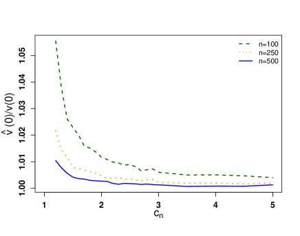
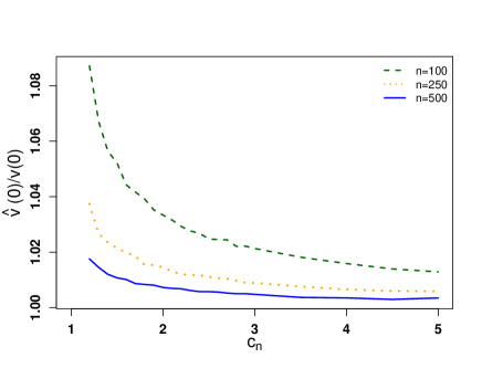
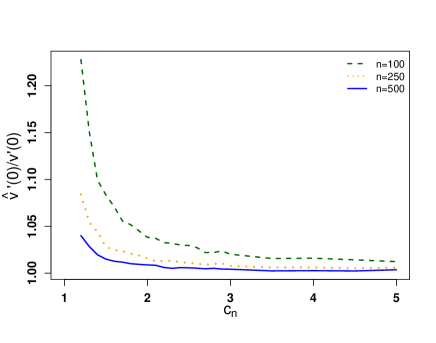
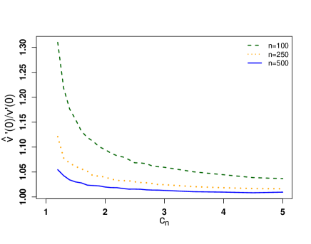
Figure 1: Finite-sample performance of the estimators for $v(0)$ and $v^{\prime}(0)$ when $c_{n}\in(1,5]$, $n\in\{100,250,500\}$, and the elements of $\mathbf{X}_{n}$ drawn from the normal distribution (first column) and scale $t$-distribution (second column).

In Corollary 2.3, we compute the closed-form expressions in case $m=1,2,3,4$.

Corollary 2.3.

Let $\mathbf{Y}_{n}$ fulfill the stochastic representation (2.1).Then, under Assumptions (A1)-(A3) we get (2.4) with

$$s_{1}(\mathbf{\Theta}) = -v^{\prime}(0)d_{1}(\mathbf{\Theta}),$$

$$s_{2}(\mathbf{\Theta}) = \frac{1}{2}v^{\prime\prime}(0)d_{1}(\mathbf{\Theta})-[v^{\prime}(0)]^{2}d_{2}(\mathbf{\Theta}),$$

$$s_{3}(\mathbf{\Theta}) = -\frac{1}{6}v^{\prime\prime\prime}(0)d_{1}(\mathbf{\Theta})+v^{\prime}(0)v^{\prime\prime}(0)d_{2}(\mathbf{\Theta})-[v^{\prime}(0)]^{3}d_{3}(\mathbf{\Theta}),$$

$$s_{4}(\mathbf{\Theta}) = \frac{1}{24}v^{\prime\prime\prime\prime}(0)d_{1}(\mathbf{\Theta})-\frac{1}{12}\left(4v^{\prime}(0)v^{\prime\prime\prime}(0)+3[v^{\prime\prime}(0)]^{2}\right)d_{2}(\mathbf{\Theta})$$

$$+\frac{3}{2}[v^{\prime}(0)]^{2}v^{\prime\prime}(0)d_{3}(\mathbf{\Theta})-[v^{\prime}(0)]^{4}d_{4}(\mathbf{\Theta}),$$

for $\quad p/n\rightarrow c\in(1,\infty)$ as $n\rightarrow\infty$ with where $v(0)$ is the unique solution of (2.7),

$$v^{\prime}(0) = -h^{-1}_{2},$$

$$v^{\prime\prime}(0) = -2[v^{\prime}(0)]^{3}h_{3},$$

$$v^{\prime\prime\prime}(0) = -6[v^{\prime}(0)]^{2}v^{\prime\prime}(0)h_{3}+6[v^{\prime}(0)]^{4}h_{4},$$

$$v^{\prime\prime\prime\prime}(0) = -\left(8[v^{\prime}(0)]^{2}v^{\prime\prime\prime}(0)+6v^{\prime}(0)[v^{\prime\prime}(0)]^{2}\right)h_{3}+36[v^{\prime}(0)]^{3}v^{\prime\prime}(0)h_{4}-24[v^{\prime}(0)]^{5}h_{5},$$

and $d_{k}(\mathbf{\Theta})$ and $h_{k}$ defined in (2.6) and (2.10), respectively.

Next, we present the general results of Theorem 2.1 in the special case of $\mathbf{\Sigma}=\mathbf{I}_{p}$ in Corollary 2.4.

Corollary 2.4.

Let $\mathbf{Y}_{n}$ fulfill the stochastic representation (2.1) with $\mathbf{\Sigma}=\mathbf{I}_{p}$. Then, under Assumptions (A2)-(A3) it holds that

$$\left|\text{tr}((\mathbf{S}_{n}^{+})^{m}\mathbf{\Theta})-\frac{(-1)^{m-1}v^{(m-1)}(0)}{(m-1)!c_{n}}\text{tr}(\mathbf{\Theta})\right|\stackrel{{\scriptstyle a.s.}}{{\rightarrow}}0$$ (2.14)

for $p/n\rightarrow c\in(1,\infty)$ as $n\rightarrow\infty$ with

$$v(0)=\frac{1}{c_{n}-1},\quad v^{\prime}(0)=\frac{-c_{n}}{(c_{n}-1)^{3}}$$ (2.15)

and

$$v^{(m)}(0)=\frac{c_{n}}{(c_{n}-1)^{3}}\sum_{k=2}^{m}(-1)^{k}k!(c_{n}-1)^{(k+1)}\left(1-c_{n}^{-k}\right)B_{m,k}\left(v^{\prime}(0),...,v^{(m-k+1)}(0)\right).$$ (2.16)

As a special case of Corollary 2.4 we get

$$\left|\text{tr}(\mathbf{S}_{n}^{+}\mathbf{\Theta})-\frac{1}{(c_{n}-1)c_{n}}\text{tr}\left(\mathbf{\Theta}\right)\right|\stackrel{{\scriptstyle a.s.}}{{\rightarrow}}0,$$

$$\left|\text{tr}((\mathbf{S}_{n}^{+})^{2}\mathbf{\Theta})-\frac{1}{(c_{n}-1)^{3}}\text{tr}\left(\mathbf{\Theta}\right)\right|\stackrel{{\scriptstyle a.s.}}{{\rightarrow}}0,$$

$$\left|\text{tr}((\mathbf{S}_{n}^{+})^{3}\mathbf{\Theta})-\frac{c_{n}+1}{(c_{n}-1)^{5}}\text{tr}\left(\mathbf{\Theta}\right)\right|\stackrel{{\scriptstyle a.s.}}{{\rightarrow}}0,$$

$$\left|\text{tr}((\mathbf{S}_{n}^{+})^{4}\mathbf{\Theta})-\frac{c_{n}^{2}+3c_{n}+1}{(c_{n}-1)^{7}}\text{tr}\left(\mathbf{\Theta}\right)\right|\stackrel{{\scriptstyle a.s.}}{{\rightarrow}}0,$$

$\text{for}\quad p/n\rightarrow c\in(1,\infty)\quad\text{as}\quad n\rightarrow\infty$.

The results of Corollary 2.4 extend the previous findings of Cook and Forzani, (2011) and Imori and von Rosen, (2020). Under the additional assumption that the elements of the matrix $\mathbf{Y}_{n}$ are normally distributed, we get that $(n-1)\mathbf{S}_{n}$ has a $p$-dimensional singular Wishart distribution with $n-1$ degrees of freedom and identity covariance matrix (see, e.g., Srivastava, (2003), Bodnar and Okhrin, (2008)). Cook and Forzani, (2011) derived the exact expression of the mean matrix of the singular Wishart distribution under the assumption that the population covariance matrix is proportional to the identity matrix. They proved that

$$\mathbb{E}\left(\mathbf{S}_{n}^{+}\right)=(n-1)\mathbb{E}\left(((n-1)\mathbf{S}_{n})^{+}\right)=\frac{(n-1)^{2}}{p(p-n)}\mathbf{I}_{p}.$$

Furthermore, it holds that $\dfrac{(n-1)^{2}}{p(p-n)}\to\dfrac{1}{c(c-1)}$ for $p/n\to c\in(1,\infty)$ as $n\to\infty$. On the other side, the application of Corollary 2.4 leads to the same result when one defines $\mathbf{\Theta}=\mathbf{e}_{i}\mathbf{e}_{j}^{\top}$, $i,j=1,...,p$, where $\mathbf{e}_{i}$ is the vector of zeros except the $i$-th element which is one.

Imori and von Rosen, (2020) extend the results of Cook and Forzani, (2011) by considering a singular Wishart distribution with an arbitrary covariance matrix and deriving the lower and the upper limits of the mean matrix and covariance matrix. The findings of Corollary 2.4 provides further generalization by establishing the limiting behaviour of the elements of the Moore-Penrose inverse of the sample covariance matrix. Moreover, the results of Theorem 2.1, Corollary 2.2, Corollary 2.3 and Corollary 2.4 are derived in general case without the assumption of normality imposed on the elements of $\mathbf{Y}_{n}$.

2.2 Weighted moments of the sample ridge-type inverse

The proof of Theorem 2.1 can be adjusted for computing the weighted trace moments and its ridge-type inverse of the sample covariance matrix, expressed as

$$\mathbf{S}_{n}^{-}(t)=(\mathbf{S}_{n}+t\mathbf{I})^{-1}.$$ (2.17)

Theorem 2.5 presents the weighted sample moments of the ridge-type inverse.

Theorem 2.5.

Let $\mathbf{Y}_{n}$ fulfill the stochastic representation (2.1). Then, under Assumptions (A1)-(A3) for any $t>0$ and $m=0,1,2,\ldots$, it holds that

$$\left|\text{tr}((\mathbf{S}_{n}^{-}(t))^{m+1}\mathbf{\Theta})-\tilde{s}_{m+1}\left(t,\mathbf{\Theta}\right)\right|\stackrel{{\scriptstyle a.s.}}{{\rightarrow}}0\quad\text{for}\quad p/n\rightarrow c\in(1,\infty)\quad\text{as}\quad n\rightarrow\infty$$ (2.18)

where

$$\tilde{s}_{m+1}\left(t,\mathbf{\Theta}\right) = \sum_{l=1}^{m}t^{-(m-l)-1}\sum_{k=1}^{l}\frac{(-1)^{l+k}k!}{l!}d_{k}\left(t,\mathbf{\Theta}\right)B_{l,k}\left(v^{\prime}(t),v^{\prime\prime}(t),...,v^{(l-k+1)}(t)\right)$$ (2.19)

$$+ t^{-m-1}d_{0}\left(t,\mathbf{\Theta}\right)$$

with

$$d_{k}\left(t,\mathbf{\Theta}\right) = \text{tr}\left\{\left(v(t)\mathbf{\Sigma}+\mathbf{I}_{p}\right)^{-1}\left[\mathbf{\Sigma}\left(v(t)\mathbf{\Sigma}+\mathbf{I}_{p}\right)^{-1}\right]^{k}\mathbf{\Theta}\right\},\quad k=0,1,2,...,$$ (2.20)

$v(t)$ is the unique solution of the equation

$$\frac{1}{p}\text{tr}\left[\left(v(t)\mathbf{\Sigma}+\mathbf{I}_{p}\right)^{-1}\right]=\frac{c_{n}-1+tv(t)}{c_{n}},$$ (2.21)

$$v^{\prime}(t)=-\frac{1}{v(t)^{-2}-c_{n}\frac{1}{p}\text{tr}\left\{\left[\mathbf{\Sigma}\left(v(t)\mathbf{\Sigma}+\mathbf{I}_{p}\right)^{-1}\right]^{2}\right\}},$$ (2.22)

and $v^{\prime\prime}(t)$,…,$v^{(m)}(t)$ are computed recursively by

$$v^{(m)}(t)=-v^{\prime}(t)\sum_{k=2}^{m}(-1)^{k}k!h_{k+1}(t)B_{m,k}\left(v^{\prime}(t),...,v^{(m-k+1)}(t)\right),$$ (2.23)

with

$$h_{k}(t)=[v(t)]^{-k}-c_{n}\frac{1}{p}\text{tr}\left\{\left[\mathbf{\Sigma}\left(v(t)\mathbf{\Sigma}+\mathbf{I}_{p}\right)^{-1}\right]^{k}\right\},\quad k=1,2,....$$ (2.24)

It is interesting to note that $\tilde{s}_{m+1}\left(t,\mathbf{\Theta}\right)$ in (2.19) can be recursively computed by

$$\tilde{s}_{m+1}\left(t,\mathbf{\Theta}\right)=\frac{1}{t}\tilde{s}_{m}\left(t,\mathbf{\Theta}\right)+\frac{1}{t}\sum_{k=1}^{m}\frac{(-1)^{m+k}k!}{m!}d_{k}\left(t,\mathbf{\Theta}\right)B_{m,k}\left(v^{\prime}(t),v^{\prime\prime}(t),...,v^{(m-k+1)}(t)\right).$$ (2.25)

Using (2.25), we present the results in a special case for $\mathbf{\Theta}=({1}/{p})\mathbf{I}_{p}$ in Corollary 2.6.

Corollary 2.6.

Let $\mathbf{Y}_{n}$ fulfill the stochastic representation (2.1). Then, under Assumptions (A1)-(A2) for any $t>0$, it holds that

$$\left|\frac{1}{p}\text{tr}\left[(\mathbf{S}_{n}^{-}(t))^{m+1}\right]-\tilde{s}_{m+1}\left(t,\frac{1}{p}\mathbf{I}_{p}\right)\right|\stackrel{{\scriptstyle a.s.}}{{\rightarrow}}0\quad\text{for}\quad p/n\rightarrow c\in(1,\infty)\quad\text{as}\quad n\rightarrow\infty,$$

where

$$\tilde{s}_{m+1}\left(t,\frac{1}{p}\mathbf{I}_{p}\right)=t^{-(m+1)}\frac{c_{n}-1}{c_{n}}+\frac{(-1)^{m}v^{(m)}(t)}{m!c_{n}}\quad\text{for}\quad m=0,1,2,...$$ (2.26)

and $v^{(m)}(t)$, $m=0,1,...$, are defined in (2.21)-(2.23) with $v^{(0)}(t)=v(t)$.

Several interesting results follows from the statement of Corollary 2.6. The sample trace moments $\text{tr}((\mathbf{S}_{n}^{-}(t))^{m+1})$ are not defined for $t=0$, while their limiting values can be computed well approximated by the expressions of the form $at^{-(m+1)}+b(t)$, where the constant $a$ depends only on $c_{n}$. Moreover, all equations (2.21) to (2.23) in Theorem 2.5 which are used in the computations of $v^{(m)}(t)$, $m=0,1,...$, are well defined at $t=0$ and they coincide with the corresponding expressions (2.7) to (2.9) derived in Theorem 2.1 for the Moore-Penrose inverse. Finally, even though the function $v(t)$ is defined as a solution of a nonlinear equation (2.21) and it is not available in the closed form, we show that it is a decreasing function in Theorem 2.7.

Theorem 2.7.

Under the conditions in Theorem 2.5, it holds that $v(t)$ is a strictly decreasing for $t\geq 0$.

Another important application of Corollary 2.6 provides consistent estimators for $v^{(m)}(t)$, $m=0,1,...$, for $t>0$ despite these functions are not defined in the closed form in Theorem 2.5. Their consistent estimators are given by

$$\hat{v}^{(m)}(t)=(-1)^{m}m!c_{n}\left(\frac{1}{p}\text{tr}\left[(\mathbf{S}_{n}^{-}(t))^{m+1}\right]-t^{-(m+1)}\frac{c_{n}-1}{c_{n}}\right).$$ (2.27)

Figure 2 depicts the estimators of $v(t)$ and $v^{\prime}(t)$, normalized by the corresponding true values for $t\in[0.1,5]$. Two data-generating models are considered, which are the normal distribution and the scaled $t$-distribution with five degrees of freedom. The covariance matrix $\mathbf{\Sigma}$ is set following the procedure described in Section 4. In the figure we observe, that $\hat{v}(t)$ and $\hat{v}^{\prime}(t)$ converge to $v(t)$ and $v^{\prime}(t)$, respectively, already for $n=100$. The results are similar for all considered values of the concentration ratio $c_{n}$ and the distributional models used to generate $\mathbf{X}_{n}$. It is interesting that for small values of $t$, the convergence is slower.

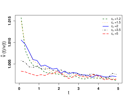
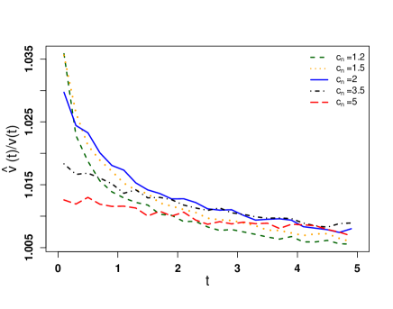
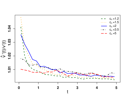
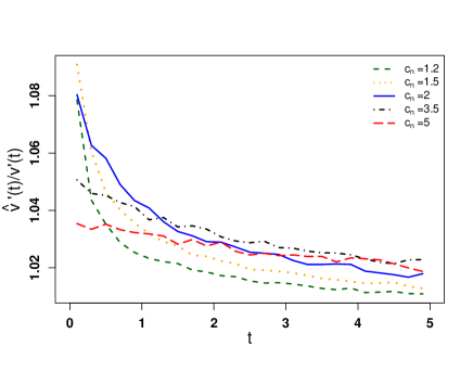
Figure 2: Finite-sample performance of the estimators for $v(t)$ and $v^{\prime}(t)$ when $t\in[0.1,5]$, $c_{n}\in\{1.2,1.5,2,3.5,5\}$, $n=100$, and the elements of $\mathbf{X}_{n}$ drawn from the normal distribution (first column) and scale $t$-distribution (second column).

In Corollaries 2.8 and 2.9, several results are presented in important special cases. Namely, Corollary 2.8 provides the formulae for $\tilde{s}_{m}\left(t,\mathbf{\Theta}\right)$ for $m=1,2,3,4$, while Corollary 2.9 presents the findings under the additional assumption that the true population covariance matrix is the identity matrix.

Corollary 2.8.

Let $\mathbf{Y}_{n}$ fulfill the stochastic representation (2.1). Then, under Assumptions (A1)-(A3) for any $t>0$, we get (2.4) with

$$\tilde{s}_{1}\left(t,\mathbf{\Theta}\right) = t^{-1}d_{0}(t,\mathbf{\Theta}),$$

$$\tilde{s}_{2}\left(t,\mathbf{\Theta}\right) = t^{-2}d_{0}(t,\mathbf{\Theta})+t^{-1}v^{\prime}(t)d_{1}(t,\mathbf{\Theta}),$$

$$\tilde{s}_{3}\left(t,\mathbf{\Theta}\right) = t^{-3}d_{0}(t,\mathbf{\Theta})+t^{-2}v^{\prime}(t)d_{1}(t,\mathbf{\Theta})+t^{-1}\left\{[v^{\prime}(t)]^{2}d_{2}(t,\mathbf{\Theta})-\frac{1}{2}v^{\prime\prime}(t)d_{1}(t,\mathbf{\Theta})\right\},$$

$$\tilde{s}_{4}\left(t,\mathbf{\Theta}\right) = t^{-4}d_{0}(t,\mathbf{\Theta})+t^{-3}v^{\prime}(t)d_{1}(t,\mathbf{\Theta})+t^{-2}\left\{[v^{\prime}(t)]^{2}d_{2}(t,\mathbf{\Theta})-\frac{1}{2}v^{\prime\prime}(t)d_{1}(t,\mathbf{\Theta})\right\}$$

$$+t^{-1}\left\{\frac{1}{6}v^{\prime\prime\prime}(t)d_{1}(t,\mathbf{\Theta})-v^{\prime}(t)v^{\prime\prime}(t)d_{2}(t,\mathbf{\Theta})+[v^{\prime}(t)]^{3}d_{3}(t,\mathbf{\Theta})\right\},$$

for $p/n\rightarrow c\in(1,\infty)$ as $n\rightarrow\infty$ where $d_{k}\left(t,\mathbf{\Theta}\right)$ and $h_{k}(t)$ are defined in (2.20) and (2.24), $v(t)$ is the unique solution of (2.21) and

$$v^{\prime}(t) = -h_{2}(t)^{-1},$$

$$v^{\prime\prime}(t) = -2[v^{\prime}(t)]^{3}h_{3}(t),$$

$$v^{\prime\prime\prime}(t) = -6[v^{\prime}(t)]^{2}v^{\prime\prime}(t)h_{3}(t)+6[v^{\prime}(t)]^{4}h_{4}(t).$$

Corollary 2.9.

Let $\mathbf{Y}_{n}$ fulfill the stochastic representation (2.1) with $\mathbf{\Sigma}=\mathbf{I}_{p}$. Then, under Assumptions (A2)-(A3) for any $t>0$, it holds that

$$\left|\text{tr}((\mathbf{S}_{n}^{-}(t))^{m+1}\mathbf{\Theta})-\left(t^{-(m+1)}\frac{c_{n}-1}{c_{n}}+\frac{(-1)^{m}v^{(m)}(t)}{m!c_{n}}\right)\text{tr}(\mathbf{\Theta})\right|\stackrel{{\scriptstyle a.s.}}{{\rightarrow}}0$$ (2.28)

for $p/n\rightarrow c\in(1,\infty)$ as $n\rightarrow\infty$ with

$$v(t)=\frac{2}{(c_{n}-1+t)+\sqrt{(c_{n}-1+t)^{2}+4t}},\quad v^{\prime}(t)=\frac{-1}{v(t)^{-2}-c_{n}(v(t)+1)^{-2}}$$ (2.29)

and

$$v^{(m)}(t)=-v^{\prime}(t)\sum_{k=2}^{m}(-1)^{k}k!\left(v(t)^{-(k+1)}-c_{n}(v(t)+1)^{-(k+1)}\right)B_{m,k}\left(v^{\prime}(t),...,v^{(m-k+1)}(t)\right).$$ (2.30)

2.3 Weighted moments of the sample Moore-Penrose-ridge inverse

Taking into account the properties of the Moore-Penrose and ridge-type inverses one can take the advantage of both estimators and build a new inverse for any $t>0$ by

$$\mathbf{S}^{\pm}_{n}(t)=(\mathbf{S}_{n}+t\mathbf{I})^{-1}\mathbf{S}_{n}(\mathbf{S}_{n}+t\mathbf{I})^{-1}\,.$$ (2.31)

This matrix inherits the properties of the Moore-Penrose inverse for $t\to 0$ because by the spectral decomposition, we have

$$\lim\limits_{t\to 0}\mathbf{S}^{\pm}_{n}(t) = \lim\limits_{t\to 0}(\mathbf{S}_{n}+t\mathbf{I})^{-1}\mathbf{S}_{n}(\mathbf{S}_{n}+t\mathbf{I})^{-1}=\lim\limits_{t\to 0}\mathbf{U}\text{diag}\left\{\frac{d_{1}}{(d_{1}+t)^{2}},\ldots,\frac{d_{p}}{(d_{p}+t)^{2}}\right\}\mathbf{U}^{\top}=\mathbf{S}_{n}^{+},$$

where $\mathbf{S}_{n}=\mathbf{U}\text{diag}\left\{d_{1},...,d_{p}\right\}\mathbf{U}^{\top}$ is the spectral decomposition of $\mathbf{S}_{n}$.

On the other side, it is related to the ridge inverse since

$$\mathbf{S}^{\pm}_{n}(t) = (\mathbf{S}_{n}+t\mathbf{I})^{-1}-t(\mathbf{S}_{n}+t\mathbf{I})^{-2}.$$ (2.32)

In fact, we have already all of the instruments to find the asymptotic behaviour for the weighted moments of $\mathbf{S}^{\pm}(t)$. Indeed, using binomial theorem we get

$$(\mathbf{S}^{\pm}_{n}(t))^{m} = \left((\mathbf{S}_{n}+t\mathbf{I})^{-1}-t(\mathbf{S}_{n}+t\mathbf{I})^{-2}\right)^{m}=\sum\limits_{k=0}^{m}\binom{m}{k}(\mathbf{S}_{n}+t\mathbf{I})^{-(m-k)}(-1)^{k}t^{k}(\mathbf{S}_{n}+t\mathbf{I})^{-2k}$$ (2.33)

$$= \sum\limits_{k=0}^{m}(-1)^{k}t^{k}\binom{m}{k}(\mathbf{S}_{n}+t\mathbf{I})^{-(m+k)}\,.$$

Thus, in order to find the limit of $\text{tr}\left((\mathbf{S}^{\pm}_{n}(t))^{m}\mathbf{\Theta}\right)$ we only need to know the limits of the functionals $\text{tr}\left((\mathbf{S}_{n}+t\mathbf{I})^{-(m+k)}\mathbf{\Theta}\right)$, which have already been derived in Theorem 2.5. As a result, we get the following results.

Theorem 2.10.

Let $\mathbf{Y}_{n}$ fulfill the stochastic representation (2.1). Then, under Assumptions (A1)-(A3) for any $t>0$ and $m=1,2,\ldots,$ it holds that

$$\left|\text{tr}((\mathbf{S}_{n}^{\pm}(t))^{m}\mathbf{\Theta})-\grave{s}_{m}\left(t,\mathbf{\Theta}\right)\right|\stackrel{{\scriptstyle a.s.}}{{\rightarrow}}0\quad\text{for}\quad p/n\rightarrow c\in(1,\infty)\quad\text{as}\quad n\rightarrow\infty$$

with

$$\grave{s}_{m}\left(t,\mathbf{\Theta}\right) = \sum\limits_{k=0}^{m}(-1)^{k}t^{k}\binom{m}{k}\tilde{s}_{m+k}(t,\mathbf{\Theta})\,,$$ (2.34)

where $\tilde{s}_{m+k}(t,\mathbf{\Theta})$ can be computed using (2.19) for $k=0,1,\ldots,m$ and $m=1,2,\ldots$.

In Corollary 2.11 we present another expression of $\grave{s}_{m}(t,\mathbf{\Theta})$ which follows from the recursive computation of $\tilde{s}_{m+k}(t,\mathbf{\Theta})$ as given in (2.25). The proof of Corollary 2.11 is given in the appendix.

Corollary 2.11.

Let $\mathbf{Y}_{n}$ fulfill the stochastic representation (2.1). Then, under Assumptions (A1)-(A3) for any $t>0$, it holds that

$$\grave{s}_{m}\left(t,\mathbf{\Theta}\right) = -D_{m}(t,\mathbf{\Theta})+\sum\limits_{k=2}^{m}(-1)^{k}\binom{m}{k}\sum\limits_{j=1}^{k-1}t^{j}D_{m+j}(t,\mathbf{\Theta})\,,$$ (2.35)

where

$$D_{m}(t,\mathbf{\Theta})=\sum_{k=1}^{m}\frac{(-1)^{m+k}k!}{m!}d_{k}\left(t,\mathbf{\Theta}\right)B_{m,k}\left(v^{\prime}(t),v^{\prime\prime}(t),...,v^{(m-k+1)}(t)\right).$$ (2.36)

Interestingly, the summands which were unbounded for $\tilde{s}_{m}(t,\mathbf{\Theta})$ as $t\to 0$ are all canceled in the limiting behavior of for $\grave{s}_{m}(t,\mathbf{\Theta})$. Since all derivatives of $v(t)$ and the functions $d_{k}(t,\mathbf{\Theta})$ for $k\geq 1$ are all well-defined and bounded in $t=0$, it holds that the limits of $\grave{s}_{m}(t,\mathbf{\Theta})$ are also well defined at zero and, moreover,

$$\grave{s}_{m}(0,\mathbf{\Theta})=-D_{m}(0,\mathbf{\Theta})=s_{m}(\mathbf{\Theta}).$$

Hence, the limiting behavior of $\grave{s}_{m}(0,\mathbf{\Theta})$ coincides with the one, obtained in the case of the Moore-Penrose inverse.

Next, we present the results in the special case of $\mathbf{\Theta}=(1/p)\mathbf{I}_{p}$.

Corollary 2.12.

Let $\mathbf{Y}_{n}$ fulfill the stochastic representation (2.1). Then, under Assumptions (A1)-(A2) for any $t>0$, it holds that

$$\left|\frac{1}{p}\text{tr}\left[(\mathbf{S}_{n}^{\pm}(t))^{m}\right]-\grave{s}_{m}\left(t,\frac{1}{p}\mathbf{I}_{p}\right)\right|\stackrel{{\scriptstyle a.s.}}{{\rightarrow}}0\quad\text{for}\quad p/n\rightarrow c\in(1,\infty)\quad\text{as}\quad n\rightarrow\infty,$$

where

$$\grave{s}_{m}\left(t,\frac{1}{p}\mathbf{I}_{p}\right)=\frac{(-1)^{m-1}}{c_{n}}\sum\limits_{k=0}^{m}\binom{m}{k}\frac{v^{(m+k-1)}(t)}{(m+k-1)!}t^{k}\quad\text{for}\quad m=1,2,...$$ (2.37)

and $v^{(m)}(t)$, $m=0,1,...$, are defined in (2.21)-(2.23) with $v^{(0)}(t)=v(t)$.

The proof of Corollary 2.12 is given in the appendix. The results in two other important special cases are summarized in Corollaries 2.13 and 2.14

Corollary 2.13.

Let $\mathbf{Y}_{n}$ fulfill the stochastic representation (2.1). Then, under Assumptions (A1)-(A3) for any $t>0$ we get (2.4) with

$$\grave{s}_{1}\left(t,\mathbf{\Theta}\right) = -v^{\prime}(t)d_{1}\left(t,\mathbf{\Theta}\right),$$ (2.38)

$$\grave{s}_{2}\left(t,\mathbf{\Theta}\right) = -\left\{[v^{\prime}(t)]^{2}d_{2}(t,\mathbf{\Theta})-\frac{1}{2}v^{\prime\prime}(t)d_{1}(t,\mathbf{\Theta})\right\}$$ (2.39)

$$+ t\left\{\frac{1}{6}v^{\prime\prime\prime}(t)d_{1}(t,\mathbf{\Theta})-v^{\prime}(t)v^{\prime\prime}(t)d_{2}(t,\mathbf{\Theta})+[v^{\prime}(t)]^{3}d_{3}(t,\mathbf{\Theta})\right\},$$

for $p/n\rightarrow c\in(1,\infty)$ as $n\rightarrow\infty$ where $d_{k}\left(t,\mathbf{\Theta}\right)$ and $h_{k}(t)$ are defined in (2.20) and (2.24), and $v^{(m)}(t)$, $m=0,1,...$, are defined in (2.21)-(2.23) with $v^{(0)}(t)=v(t)$.

Corollary 2.14.

Let $\mathbf{Y}_{n}$ fulfill the stochastic representation (2.1) with $\mathbf{\Sigma}=\mathbf{I}_{p}$. Then, under Assumptions (A2)-(A3) for any $t>0$, it holds that

$$\left|\text{tr}((\mathbf{S}_{n}^{\pm}(t))^{m+1}\mathbf{\Theta})-\frac{(-1)^{m-1}}{c_{n}}\sum\limits_{k=0}^{m}\binom{m}{k}\frac{v^{(m+k-1)}(t)}{(m+k-1)!}t^{k}\text{tr}(\mathbf{\Theta})\right|\stackrel{{\scriptstyle a.s.}}{{\rightarrow}}0$$ (2.40)

for $p/n\rightarrow c\in(1,\infty)$ as $n\rightarrow\infty$ with $v(t)$ and $v^{(m)}(t)$ defined in (2.29) and (2.30).

2.4 Weighted moments of sample covariance matrix

In this section, we present the results for the weighted trace moments of the sample covariance matrix. The results of this section are established in both cases $p/n>1$ and $p/n<1$.

Theorem 2.15.

Let $\mathbf{Y}_{n}$ fulfill the stochastic representation (2.1). Then, under Assumptions (A1)-(A3), it holds that

$$\left|\text{tr}(\mathbf{S}_{n}^{m}\mathbf{\Theta})-\breve{s}_{m}(\mathbf{\Theta})\right|\stackrel{{\scriptstyle a.s.}}{{\rightarrow}}0\quad\text{for}\quad p/n\rightarrow c\in[0,\infty)\quad\text{as}\quad n\rightarrow\infty$$ (2.41)

where

$$\breve{s}_{m}(\mathbf{\Theta}) = \sum_{k=1}^{m}\frac{(-1)^{m+k}k!}{m!}\text{tr}\left\{\mathbf{\Sigma}^{k}\mathbf{\Theta}\right\}B_{m,k}\left(u^{\prime}(0),u^{\prime\prime}(0),...,u^{(m-k+1)}(0)\right),$$ (2.42)

$u^{\prime}(0)=1$ and $u^{\prime\prime}(0)$,…,$u^{(m)}(0)$ are computed recursively by

$$u^{(m)}(0)=mc_{n}\sum_{k=1}^{m-1}\frac{(-1)^{k}k!}{p}\text{tr}\left\{\mathbf{\Sigma}^{k}\right\}B_{m-1,k}\left(u^{\prime}(0),...,u^{(m-k)}(0)\right).$$ (2.43)

In Corollary 2.16 we present the results derived for $\mathbf{\Theta}=\frac{1}{p}\mathbf{I}_{p}$.

Corollary 2.16.

Let $\mathbf{Y}_{n}$ fulfill the stochastic representation (2.1). Then, under Assumptions (A1)-(A2), it holds that

$$\left|\frac{1}{p}\text{tr}\left[\mathbf{S}_{n}^{m}\right]-\breve{s}_{m+1}\left(\frac{1}{p}\mathbf{I}_{p}\right)\right|\stackrel{{\scriptstyle a.s.}}{{\rightarrow}}0\quad\text{for}\quad p/n\rightarrow c\in(0,\infty)\quad\text{as}\quad n\rightarrow\infty,$$

where

$$\breve{s}_{m+1}\left(\frac{1}{p}\mathbf{I}_{p}\right)=\frac{(-1)^{m}u^{(m+1)}(0)}{(m+1)!c_{n}}\quad\text{for}\quad m=1,2,...$$ (2.44)

and $u^{m}(0)$, $m=1,...$, are defined in (2.43).

Corollary 2.17.

Let $\mathbf{Y}_{n}$ fulfill the stochastic representation (2.1). Then, under Assumptions (A1)-(A3), we get (2.4) with

$$\breve{s}_{1}(\mathbf{\Theta}) = \text{tr}(\mathbf{\Sigma}\mathbf{\Theta}),$$

$$\breve{s}_{2}(\mathbf{\Theta}) = c_{n}\frac{1}{p}\text{tr}(\mathbf{\Sigma})\text{tr}(\mathbf{\Sigma}\mathbf{\Theta})+\text{tr}(\mathbf{\Sigma}^{2}\mathbf{\Theta}),$$

$$\breve{s}_{3}(\mathbf{\Theta}) = c_{n}\left\{c_{n}\left[\frac{1}{p}\text{tr}(\mathbf{\Sigma})\right]^{2}+\frac{1}{p}\text{tr}(\mathbf{\Sigma}^{2})\right\}\text{tr}(\mathbf{\Sigma}\mathbf{\Theta})+2c_{n}\frac{1}{p}\text{tr}(\mathbf{\Sigma})\text{tr}(\mathbf{\Sigma}^{2}\mathbf{\Theta})+\text{tr}(\mathbf{\Sigma}^{3}\mathbf{\Theta}),$$

$$\breve{s}_{4}(\mathbf{\Theta}) = c_{n}\left\{c_{n}^{2}\left[\frac{1}{p}\text{tr}(\mathbf{\Sigma})\right]^{3}+3c_{n}\frac{1}{p}\text{tr}(\mathbf{\Sigma})\frac{1}{p}\text{tr}(\mathbf{\Sigma}^{2})+\frac{1}{p}\text{tr}(\mathbf{\Sigma}^{3})\right\}\text{tr}(\mathbf{\Sigma}\mathbf{\Theta})$$

$$+c_{n}\left\{3c_{n}\left[\frac{1}{p}\text{tr}(\mathbf{\Sigma})\right]^{2}+2\frac{1}{p}\text{tr}(\mathbf{\Sigma}^{2})\right\}\text{tr}(\mathbf{\Sigma}^{2}\mathbf{\Theta})+3c_{n}\frac{1}{p}\text{tr}(\mathbf{\Sigma})\text{tr}(\mathbf{\Sigma}^{3}\mathbf{\Theta})+\text{tr}(\mathbf{\Sigma}^{4}\mathbf{\Theta}),$$

for $p/n\rightarrow c\in[0,\infty)$ as $n\rightarrow\infty$.

Corollary 2.18.

Let $\mathbf{Y}_{n}$ fulfill the stochastic representation (2.1) with $\mathbf{\Sigma}=\mathbf{I}_{p}$. Then, under Assumptions (A2)-(A3), it holds that

$$\left|\text{tr}(\mathbf{S}_{n}^{m}\mathbf{\Theta})-\frac{(-1)^{m}u^{(m+1)}(0)}{(m+1)!c_{n}}\text{tr}\left\{\mathbf{\Theta}\right\}\right|\stackrel{{\scriptstyle a.s.}}{{\rightarrow}}0$$ (2.45)

for $p/n\rightarrow c\in(0,\infty)$ as $n\rightarrow\infty$, where $u^{(m+1)}(0)$, $m=1,...$, are given in (2.43) with $\mathbf{\Sigma}=\mathbf{I}_{p}$.

As a special case of Corollary 2.18 we get

$$\left|\text{tr}(\mathbf{S}_{n}\mathbf{\Theta})-\text{tr}\left(\mathbf{\Theta}\right)\right|\stackrel{{\scriptstyle a.s.}}{{\rightarrow}}0,$$

$$\left|\text{tr}(\mathbf{S}_{n}^{2}\mathbf{\Theta})-(c_{n}+1)\text{tr}\left(\mathbf{\Theta}\right)\right|\stackrel{{\scriptstyle a.s.}}{{\rightarrow}}0,$$

$$\left|\text{tr}(\mathbf{S}_{n}^{3}\mathbf{\Theta})-(c_{n}^{2}+3c_{n}+1)\text{tr}\left(\mathbf{\Theta}\right)\right|\stackrel{{\scriptstyle a.s.}}{{\rightarrow}}0,$$

$$\left|\text{tr}(\mathbf{S}_{n}^{4}\mathbf{\Theta})-(c_{n}^{3}+6c_{n}^{2}+6c_{n}+1)\text{tr}\left(\mathbf{\Theta}\right)\right|\stackrel{{\scriptstyle a.s.}}{{\rightarrow}}0,$$

for $p/n\rightarrow c\in(0,\infty)$ as $n\rightarrow\infty$.

3 Shrinkage estimator of the high-dimensional precision matrix

The results of Theorem 2.1 have a lot of applications in high-dimensional statistics. Maybe the most obvious one would be the approximation of the weighted functionals alike $\operatorname{tr}\left(f(\mathbf{S}_{n}^{+})\mbox{\boldmath$\theta$}\right)$ by Taylor expansion up to a specific order $m$, assuming that the test function $f:\mathbbm{R}\to\mathbbm{R}$ is smooth enough.

The findings of Corollary 2.2 provide the closed-form formulas for the consistent estimators of $v^{(m)}(0)$ for $m=0,1,...$ as summarized in (2.13). Using these results, we get consistent estimators for $h_{m}$ and $d_{m}\left(\frac{1}{p}\mathbf{I}_{p}\right)$ for $m=1,2,...$. In particular, consistent estimators for $h_{2}$, $h_{3}$, $d_{1}\left(\frac{1}{p}\mathbf{I}_{p}\right)$ and $d_{2}\left(\frac{1}{p}\mathbf{I}_{p}\right)$ are given by

$$\hat{h}_{2} = -\frac{1}{\hat{v}^{\prime}(0)}=\frac{1}{c_{n}\frac{1}{p}\text{tr}\left[(\mathbf{S}_{n}^{+})^{2}\right]},$$ (3.1)

$$\hat{h}_{3} = \frac{-\hat{v}^{\prime\prime}(0)}{2[\hat{v}^{\prime}(0)]^{3}}=\frac{\frac{1}{p}\text{tr}\left[(\mathbf{S}_{n}^{+})^{3}\right]}{c_{n}^{2}\left\{\frac{1}{p}\text{tr}\left[(\mathbf{S}_{n}^{+})^{2}\right]\right\}^{3}},$$ (3.2)

$$\hat{d}_{1}\left(\frac{1}{p}\mathbf{I}_{p}\right) = -\frac{\hat{s}_{1}\left(\frac{1}{p}\mathbf{I}_{p}\right)}{\hat{v}^{\prime}(0)}=\frac{\frac{1}{p}\text{tr}\left[\mathbf{S}_{n}^{+}\right]}{c_{n}\frac{1}{p}\text{tr}\left[(\mathbf{S}_{n}^{+})^{2}\right]},$$ (3.3)

$$\hat{d}_{1}\left(\frac{1}{p}\bm{\Pi}_{0}\right) = -\frac{\hat{s}_{1}\left(\frac{1}{p}\bm{\Pi}_{0}\right)}{\hat{v}^{\prime}(0)}=\frac{\frac{1}{p}\text{tr}\left[\mathbf{S}_{n}^{+}\bm{\Pi}_{0}\right]}{c_{n}\frac{1}{p}\text{tr}\left[(\mathbf{S}_{n}^{+})^{2}\right]},$$ (3.4)

$$\hat{d}_{2}\left(\frac{1}{p}\mathbf{I}_{p}\right) = \!\!\frac{\frac{1}{2}\hat{v}^{\prime\prime}(0)\hat{d}_{1}\left(\frac{1}{p}\mathbf{I}_{p}\right)-\hat{s}_{2}\left(\frac{1}{p}\mathbf{I}_{p}\right)}{[\hat{v}^{\prime}(0)]^{2}}=\frac{\frac{1}{p}\text{tr}\left[\mathbf{S}_{n}^{+}\right]\frac{1}{p}\text{tr}\left[(\mathbf{S}_{n}^{+})^{3}\right]-\left\{\frac{1}{p}\text{tr}\left[(\mathbf{S}_{n}^{+})^{2}\right]\right\}^{2}}{c_{n}^{2}\left\{\frac{1}{p}\text{tr}\left[(\mathbf{S}_{n}^{+})^{2}\right]\right\}^{3}}.$$ (3.5)

Similarly, the findings of Theorem 2.5 and Theorem 2.15 lead to the consistent estimators of $d_{0}(t,\mathbf{\Theta})$, $d_{1}(t,\mathbf{\Theta})$, $q_{1}(\mathbf{\Theta})=\text{tr}\left[\mathbf{\Sigma}\mathbf{\Theta}\right]$ and $q_{2}(\mathbf{\Theta})=\text{tr}\left[\mathbf{\Sigma}^{2}\mathbf{\Theta}\right]$ expressed as

$$\hat{d}_{0}(t,\mathbf{\Theta}) = t\leavevmode\nobreak\ \text{tr}\left[(\mathbf{S}_{n}+t\mathbf{I}_{p})^{-1}\mathbf{\Theta}\right]\quad\text{for}\quad t>0,$$ (3.6)

$$\hat{d}_{1}(t,\mathbf{\Theta}) = -\frac{t\text{tr}\left[(\mathbf{S}_{n}+t\mathbf{I}_{p})^{-2}\mathbf{\Theta}\right]-t^{-1}\hat{d}_{0}(t,\mathbf{\Theta})}{c_{n}\left(\frac{1}{p}\text{tr}\left[(\mathbf{S}_{n}+t\mathbf{I}_{p})^{-2}\right]-t^{-2}\frac{c_{n}-1}{c_{n}}\right)}\quad\text{for}\quad t>0,$$ (3.7)

$$\hat{q}_{1}(\mathbf{\Theta}) = \text{tr}\left[\mathbf{S}_{n}\mathbf{\Theta}\right],$$ (3.8)

$$\hat{q}_{2}(\mathbf{\Theta}) = \text{tr}\left[\mathbf{S}_{n}^{2}\mathbf{\Theta}\right]-c_{n}\frac{1}{p}\text{tr}\left[\mathbf{S}_{n}\right]\text{tr}\left[\mathbf{S}_{n}\mathbf{\Theta}\right].$$ (3.9)

We use the above formulas in the derivation of new shrinkage estimators of the high-dimensional precision matrix when $n<p$.

Following Bodnar et al., (2016) the general linear shrinkage estimator (GLSE) for the precision matrix is constructed by

$$\widehat{\bm{\Pi}}_{GSE}=\alpha_{n}\mathbf{S}_{n}^{\#}(t)+\beta_{n}\bm{\Pi}_{0}\,,$$ (3.10)

where $\bm{\Pi}_{0}$ is a target matrix, which typically is chosen to be equal to the identity matrix when no a priori information about the precision matrix $\mathbf{\Sigma}^{-1}$ is available. The symbol $\mathbf{S}_{n}^{\#}(t)$ denotes an estimator of the precision matrix. Later on, we choose $\mathbf{S}_{n}^{\#}(t)$ to be one of the three pseudo-inverses considered in Section 2, i.e., $\mathbf{S}_{n}^{\#}(t)\in\{\mathbf{S}_{n}^{+},\mathbf{S}_{n}^{-}(t),\mathbf{S}_{n}^{\pm}(t)\}$.

Potentially, the estimator (3.10) is nonlinear since all the three pseudo-inverses of $\mathbf{S}_{n}$ are nonlinear functions of $\mathbf{\Sigma}$ and also they are nonlinear functions of the eigenvalues of $\mathbf{S}_{n}$. For example, the Moore-Penrose inverse inverts the non-zero eigenvalues and keeps zero eigenvalues untouched. A similar structure as (3.10) obeys the non-linear quadratic shrinkage estimator of Ledoit and Wolf, (2022) with specific $\alpha_{n}$, $\beta_{n}$ and the data-driven equivariant (with same eigenvectors as $\mathbf{S}_{n}$) target $\bm{\Pi}_{0}$, which come from the nonlinear Ledoit-Péché shrinkage formula (see, Ledoit and Péché, , 2011). A proper shrinkage of $\mathbf{S}_{n}^{\#}(t)$ could result in a better estimator of $\mathbf{\Sigma}^{-1}$. Moreover, it is interesting how it compares to the well-established nonlinear shrinkage technique. The choice of $\bm{\Pi}_{0}$ is free to some extent but we will concentrate us on $\bm{\Pi}_{0}=\mathbf{I}$ in simulations to have a fair comparison with common rotation-equivariant estimators (see, e.g., Ledoit and Wolf, , 2004, 2012; Bodnar et al., , 2014).

The optimal shrinkage intensities $\alpha^{*}_{n}$ and $\beta^{*}_{n}$ are determined by minimizing the Frobenius (quadratic) loss for a given nonrandom target matrix $\bm{\Pi}_{0}$ given by (see, e.g., Haff, , 1979; Krishnamoorthy and Gupta, , 1989; Yang and Berger, , 1994; Wang et al., , 2015; Bodnar et al., , 2016)

$$L^{2}_{F;n} = ||\widehat{\bm{\Pi}}_{GSE}\mathbf{\Sigma}-\mathbf{I}||_{F}^{2}=\operatorname{tr}\left[(\widehat{\bm{\Pi}}_{GSE}\mathbf{\Sigma}-\mathbf{I})(\widehat{\bm{\Pi}}_{GSE}\mathbf{\Sigma}-\mathbf{I})^{\top}\right]$$ (3.11)

$$=||\mathbf{I}||^{2}_{F}+\alpha_{n}^{2}||\mathbf{S}_{n}^{\#}(t)\mathbf{\Sigma}||^{2}_{F}+2\alpha_{n}\beta_{n}\text{tr}(\mathbf{S}_{n}^{\#}(t)\mathbf{\Sigma}^{2}\bm{\Pi}_{0})+\beta_{n}^{2}||\bm{\Pi}_{0}\mathbf{\Sigma}||^{2}_{F}-2\alpha_{n}\text{tr}(\mathbf{S}_{n}^{\#}(t)\mathbf{\Sigma})-2\beta_{n}\text{tr}(\mathbf{\Sigma}\bm{\Pi}_{0})$$

$$= ||\mathbf{I}||^{2}_{F}+||\mathbf{S}_{n}^{\#}(t)\mathbf{\Sigma}||^{2}_{F}\left(\alpha_{n}+\frac{\beta_{n}\text{tr}(\mathbf{S}_{n}^{\#}(t)\mathbf{\Sigma}^{2}\bm{\Pi}_{0})-\text{tr}(\mathbf{S}_{n}^{\#}(t)\mathbf{\Sigma})}{||\mathbf{S}_{n}^{\#}(t)\mathbf{\Sigma}||^{2}_{F}}\right)^{2}$$

$$+ \frac{||\mathbf{S}_{n}^{\#}(t)\mathbf{\Sigma}||^{2}_{F}||\bm{\Pi}_{0}\mathbf{\Sigma}||^{2}_{F}-\left(\text{tr}(\mathbf{S}_{n}^{\#}(t)\mathbf{\Sigma}^{2}\bm{\Pi}_{0})\right)^{2}}{||\mathbf{S}_{n}^{\#}(t)\mathbf{\Sigma}||^{2}_{F}}$$

$$\times \left(\beta_{n}+\frac{\text{tr}(\mathbf{S}_{n}^{\#}(t)\mathbf{\Sigma}^{2}\bm{\Pi}_{0})\text{tr}(\mathbf{S}_{n}^{\#}(t)\mathbf{\Sigma})-||\mathbf{S}_{n}^{\#}(t)\mathbf{\Sigma}||^{2}_{F}\text{tr}(\mathbf{\Sigma}\bm{\Pi}_{0})}{||\mathbf{S}_{n}^{\#}(t)\mathbf{\Sigma}||^{2}_{F}||\bm{\Pi}_{0}\mathbf{\Sigma}||^{2}_{F}-\left(\text{tr}(\mathbf{S}_{n}^{\#}(t)\mathbf{\Sigma}^{2}\bm{\Pi}_{0})\right)^{2}}\right)^{2}$$

$$- \left(\frac{[\text{tr}(\mathbf{S}_{n}^{\#}(t)\mathbf{\Sigma})]^{2}}{||\mathbf{S}_{n}^{\#}(t)\mathbf{\Sigma}||^{2}_{F}}+\frac{[\text{tr}(\mathbf{S}_{n}^{\#}(t)\mathbf{\Sigma}^{2}\bm{\Pi}_{0})\text{tr}(\mathbf{S}_{n}^{\#}(t)\mathbf{\Sigma})-||\mathbf{S}_{n}^{\#}(t)\mathbf{\Sigma}||^{2}_{F}\text{tr}(\mathbf{\Sigma}\bm{\Pi}_{0})]^{2}}{||\mathbf{S}_{n}^{\#}(t)\mathbf{\Sigma}||^{2}_{F}\left[||\mathbf{S}_{n}^{\#}(t)\mathbf{\Sigma}||^{2}_{F}||\bm{\Pi}_{0}\mathbf{\Sigma}||^{2}_{F}-\left(\text{tr}(\mathbf{S}_{n}^{\#}(t)\mathbf{\Sigma}^{2}\bm{\Pi}_{0})\right)^{2}\right]}\right)\,.$$

Since $||\mathbf{S}_{n}^{\#}(t)\mathbf{\Sigma}||^{2}_{F}>0$ and $||\mathbf{S}_{n}^{\#}(t)\mathbf{\Sigma}||^{2}_{F}||\bm{\Pi}_{0}\mathbf{\Sigma}||^{2}_{F}-\left(\text{tr}(\mathbf{S}_{n}^{\#}(t)\mathbf{\Sigma}^{2}\bm{\Pi}_{0})\right)^{2}\geq 0$ with equality to zero if and only if $\mathbf{S}_{n}^{\#}(t)=\bm{\Pi}_{0}$, then, for a fixed value of the tuning parameter $t$, the loss function $L^{2}_{F;n}$ is minimized at

$$\beta_{n}^{*}(\mathbf{S}_{n}^{\#}(t))=\frac{||\mathbf{S}_{n}^{\#}(t)\mathbf{\Sigma}||^{2}_{F}\text{tr}(\mathbf{\Sigma}\bm{\Pi}_{0})-\text{tr}(\mathbf{S}_{n}^{\#}(t)\mathbf{\Sigma}^{2}\bm{\Pi}_{0})\text{tr}(\mathbf{S}_{n}^{\#}(t)\mathbf{\Sigma})}{||\mathbf{S}_{n}^{\#}(t)\mathbf{\Sigma}||^{2}_{F}||\bm{\Pi}_{0}\mathbf{\Sigma}||^{2}_{F}-\left(\text{tr}(\mathbf{S}_{n}^{\#}(t)\mathbf{\Sigma}^{2}\bm{\Pi}_{0})\right)^{2}}$$ (3.12)

$$= \dfrac{\text{tr}\left(\dfrac{\mathbf{\Sigma}\bm{\Pi}_{0}}{||\mathbf{\Sigma}\bm{\Pi}_{0}||_{F}}\right)||\mathbf{S}_{n}^{\#}(t)\mathbf{\Sigma}||^{2}_{F}-\text{tr}(\mathbf{S}_{n}^{\#}(t)\mathbf{\Sigma})\text{tr}\left(\mathbf{S}_{n}^{\#}(t)\dfrac{\mathbf{\Sigma}^{2}\bm{\Pi}_{0}}{||\mathbf{\Sigma}\bm{\Pi}_{0}||_{F}}\right)}{||\mathbf{S}_{n}^{\#}(t)\mathbf{\Sigma}||^{2}_{F}-\Bigl{[}\text{tr}\left(\mathbf{S}_{n}^{\#}(t)\dfrac{\mathbf{\Sigma}^{2}\bm{\Pi}_{0}}{||\mathbf{\Sigma}\bm{\Pi}_{0}||_{F}}\right)\Bigr{]}^{2}}||\mathbf{\Sigma}\bm{\Pi}_{0}||^{-1}_{F}\,.$$

and

$$\alpha_{n}^{*}(\mathbf{S}_{n}^{\#}(t))=\frac{\text{tr}(\mathbf{S}_{n}^{\#}(t)\mathbf{\Sigma})-\beta_{n}\text{tr}(\mathbf{S}_{n}^{\#}(t)\mathbf{\Sigma}^{2}\bm{\Pi}_{0})}{||\mathbf{S}_{n}^{\#}(t)\mathbf{\Sigma}||^{2}_{F}}$$ (3.13)

$$= \dfrac{\text{tr}(\mathbf{S}_{n}^{\#}(t)\mathbf{\Sigma})-\text{tr}\left(\dfrac{\mathbf{\Sigma}\bm{\Pi}_{0}}{||\mathbf{\Sigma}\bm{\Pi}_{0}||_{F}}\right)\text{tr}\left(\mathbf{S}_{n}^{\#}(t)\dfrac{{\mathbf{\Sigma}^{2}}\bm{\Pi}_{0}}{||\mathbf{\Sigma}\bm{\Pi}_{0}||_{F}}\right)}{||\mathbf{S}_{n}^{\#}(t)\mathbf{\Sigma}||^{2}_{F}-\Bigl{[}\text{tr}\left(\mathbf{S}_{n}^{\#}(t)\dfrac{{\mathbf{\Sigma}^{2}}\bm{\Pi}_{0}}{||\mathbf{\Sigma}\bm{\Pi}_{0}||_{F}}\right)\Bigr{]}^{2}}\,,$$

When $\mathbf{S}_{n}^{\#}(t)\in\{\mathbf{S}_{n}^{-}(t),\mathbf{S}_{n}^{\pm}(t)\}$, the last summand in (3.11) should be minimized with respect to the tuning parameter $t$. The last row in (3.11) can be written by

$$\frac{[\text{tr}(\mathbf{S}_{n}^{\#}(t)\mathbf{\Sigma})]^{2}}{||\mathbf{S}_{n}^{\#}(t)\mathbf{\Sigma}||^{2}_{F}}+\frac{[\text{tr}(\mathbf{S}_{n}^{\#}(t)\mathbf{\Sigma}^{2}\bm{\Pi}_{0})\text{tr}(\mathbf{S}_{n}^{\#}(t)\mathbf{\Sigma})-||\mathbf{S}_{n}^{\#}(t)\mathbf{\Sigma}||^{2}_{F}\text{tr}(\mathbf{\Sigma}\bm{\Pi}_{0})]^{2}}{||\mathbf{S}_{n}^{\#}(t)\mathbf{\Sigma}||^{2}_{F}\left[||\mathbf{S}_{n}^{\#}(t)\mathbf{\Sigma}||^{2}_{F}||\bm{\Pi}_{0}\mathbf{\Sigma}||^{2}_{F}-\left(\text{tr}(\mathbf{S}_{n}^{\#}(t)\mathbf{\Sigma}^{2}\bm{\Pi}_{0})\right)^{2}\right]}$$

$$= \frac{[\text{tr}(\mathbf{S}_{n}^{\#}(t)\mathbf{\Sigma})]^{2}||\bm{\Pi}_{0}\mathbf{\Sigma}||^{2}_{F}-2\text{tr}(\mathbf{S}_{n}^{\#}(t)\mathbf{\Sigma}^{2}\bm{\Pi}_{0})\text{tr}(\mathbf{S}_{n}^{\#}(t)\mathbf{\Sigma})\text{tr}(\mathbf{\Sigma}\bm{\Pi}_{0})+||\mathbf{S}_{n}^{\#}(t)\mathbf{\Sigma}||^{2}_{F}[\text{tr}(\mathbf{\Sigma}\bm{\Pi}_{0})]^{2}}{||\mathbf{S}_{n}^{\#}(t)\mathbf{\Sigma}||^{2}_{F}||\bm{\Pi}_{0}\mathbf{\Sigma}||^{2}_{F}-\left(\text{tr}(\mathbf{S}_{n}^{\#}(t)\mathbf{\Sigma}^{2}\bm{\Pi}_{0})\right)^{2}}.$$

$$= L^{2}_{F;n,2}(\mathbf{S}_{n}^{\#}(t))+\left[\text{tr}\left(\dfrac{\mathbf{\Sigma}\bm{\Pi}_{0}}{||\mathbf{\Sigma}\bm{\Pi}_{0}||_{F}}\right)\right]^{2}$$

with

$$L^{2}_{F;n,2}(\mathbf{S}_{n}^{\#}(t)) = \frac{\left[\text{tr}(\mathbf{S}_{n}^{\#}(t)\mathbf{\Sigma})-\text{tr}\left(\mathbf{S}_{n}^{\#}(t)\dfrac{{\mathbf{\Sigma}^{2}}\bm{\Pi}_{0}}{||\mathbf{\Sigma}\bm{\Pi}_{0}||_{F}}\right)\text{tr}\left(\dfrac{\mathbf{\Sigma}\bm{\Pi}_{0}}{||\mathbf{\Sigma}\bm{\Pi}_{0}||_{F}}\right)\right]^{2}}{||\mathbf{S}_{n}^{\#}(t)\mathbf{\Sigma}||^{2}_{F}-\Bigl{[}\text{tr}\left(\mathbf{S}_{n}^{\#}(t)\dfrac{{\mathbf{\Sigma}^{2}}\bm{\Pi}_{0}}{||\mathbf{\Sigma}\bm{\Pi}_{0}||_{F}}\right)\Bigr{]}^{2}}.$$ (3.14)

Then the optimal value of $t$ is found by maximizing $L^{2}_{F;n,2}(\mathbf{S}_{n}^{\#}(t))$.

It is important to note that after dividing by $p$ the numerator and denominator in the formulas for $\alpha^{*}_{n}(\mathbf{S}_{n}^{\#}(t))$, $\beta^{*}_{n}(\mathbf{S}_{n}^{\#}(t))$ and $L^{2}_{F;n,2}(\mathbf{S}_{n}^{\#}(t))$, no additional assumption on $\bm{\Pi}_{0}$ is needed since all ratios in (3.12), (3.13) and (3.14) are self-normalized. For example, by taking

$$\mathbf{\Theta}=\dfrac{\mathbf{\Sigma}\bm{\Pi}_{0}}{\sqrt{p}||\mathbf{\Sigma}\bm{\Pi}_{0}||_{F}}$$

in Corollary 2.3 and using Jensen’s inequality, we get that $\operatorname{tr}\left(\mathbf{\Theta}\right)\leq 1$. Similarly, for $\mathbf{\Theta}=\frac{1}{p}\mathbf{\Sigma}^{2}$ it holds that

$$\frac{1}{p}\operatorname{tr}(\mathbf{\Sigma}^{2})\leq\frac{p\lambda^{2}_{\max}(\mathbf{\Sigma})}{p}=\lambda^{2}_{\max}(\mathbf{\Sigma})<\infty.$$

In the same way, it can be shown that

$$\mathbf{\Theta}=\frac{1}{p}\mathbf{\Sigma}\quad\text{and}\quad\mathbf{\Theta}=\dfrac{\mathbf{\Sigma}^{2}\bm{\Pi}_{0}}{\sqrt{p}||\mathbf{\Sigma}\bm{\Pi}_{0}||_{F}}$$

possess bounded trace norms. The latter properties verify Assumption (A3).

Since $\alpha_{n}^{*}(\mathbf{S}_{n}^{\#}(t))$, $\beta_{n}^{*}(\mathbf{S}_{n}^{\#}(t))$ and $L^{2}_{F;n,2}(\mathbf{S}_{n}^{\#}(t))$ depend on the unknown population covariance matrix $\mathbf{\Sigma}$, they cannot be computed in practice and thus we refer to $\alpha_{n}^{*}(\mathbf{S}_{n}^{\#}(t))$ and $\beta_{n}^{*}(\mathbf{S}_{n}^{\#}(t))$ as the oracle estimators. In the high-dimensional singular setting, i.e., $p>n$, Bodnar et al., (2016) found the almost sure asymptotic equivalents for $\alpha_{n}^{*}(\mathbf{S}_{n}^{+})$ and $\beta_{n}^{*}(\mathbf{S}_{n}^{+})$ and estimate them consistently only in the case of $\mathbf{\Sigma}=\sigma^{2}\mathbf{I}_{p}$.

The results of Section 2 allow us to establish the limiting behaviour of $\alpha_{n}^{*}(\mathbf{S}_{n}^{\#}(t))$ and $\beta_{n}^{*}(\mathbf{S}_{n}^{\#}(t))$, and to estimate consistently their limiting values $\alpha^{*}$ and $\beta^{*}$ in a very general case. It is enough to find the exact limits of $\frac{1}{p}||\mathbf{S}_{n}^{\#}\mathbf{\Sigma}||^{2}_{F}=\frac{1}{p}\operatorname{tr}\left([\mathbf{S}_{n}^{\#}(t)]^{2}\mathbf{\Sigma}^{2}\right)$, $\frac{1}{p}\text{tr}(\mathbf{S}_{n}^{\#}(t)\mathbf{\Sigma})$ and $\frac{1}{p}\text{tr}\left(\mathbf{S}_{n}^{\#}(t)\dfrac{{\mathbf{\Sigma}^{2}}\bm{\Pi}_{0}}{||\mathbf{\Sigma}\bm{\Pi}_{0}||_{F}}\right)$ by using Corollary 2.3, Corollary 2.8 and Corollary 2.13, and to estimate them consistently, together with some other quantities which depend on the population covariance matrix, not on its inverse. Thus, it is straightforward to determine the almost sure equivalents of the optimal shrinkage intensities. We present the results in the following subsections for all three pseudo-inverses considered in Section 2.

3.1 Results for the Moore-Penrose inverse

In the case of the Moore-Penrose inverse, the optimization problem and the resulting optimal shrinkage intensities do not depend on the tuning parameter $t$. This fact simplifies considerably the construction of the optimal shrinkage estimator. Let $\alpha_{MP;n}^{*}=\alpha_{n}^{*}(\mathbf{S}_{n}^{+})$ and $\beta_{MP;n}^{*}=\beta_{n}^{*}(\mathbf{S}_{n}^{+})$. The asymptotic deterministic equivalents to $\alpha_{MP;n}^{*}$ and $\beta_{MP;n}^{*}$ are derived in Theorem 3.1 by using the results presented in Corollary 2.3.

Theorem 3.1.

Let $\mathbf{Y}_{n}$ fulfill the stochastic representation (2.1). Then, under Assumptions (A1)-(A2), it holds that

$$\left|\alpha_{MP;n}^{*}-\alpha_{MP}^{*}\right|\stackrel{{\scriptstyle a.s.}}{{\rightarrow}}0,\leavevmode\nobreak\ \leavevmode\nobreak\ \text{and}\leavevmode\nobreak\ \leavevmode\nobreak\ \left|\beta_{MP;n}^{*}-\beta_{MP}^{*}\right|\stackrel{{\scriptstyle a.s.}}{{\rightarrow}}0\leavevmode\nobreak\ \leavevmode\nobreak\ \text{for}\quad p/n\rightarrow c\in(1,\infty)\leavevmode\nobreak\ \text{as}\leavevmode\nobreak\ \leavevmode\nobreak\ n\rightarrow\infty$$

with

$$\alpha_{MP}^{*} = \dfrac{d_{1}(\mathbf{\Sigma})-d_{1}\left(\dfrac{\mathbf{\Sigma}^{2}\bm{\Pi}_{0}}{||\mathbf{\Sigma}\bm{\Pi}_{0}||_{F}}\right)\operatorname{tr}\left(\dfrac{\mathbf{\Sigma}\bm{\Pi}_{0}}{||\mathbf{\Sigma}\bm{\Pi}_{0}||_{F}}\right)}{-\dfrac{1}{h_{2}}\left(d_{2}(\mathbf{\Sigma}^{2})-d_{1}(\mathbf{\Sigma}^{2})\dfrac{h_{3}}{h_{2}}\right)-\dfrac{1}{h_{2}}d^{2}_{1}\left(\dfrac{\mathbf{\Sigma}^{2}\bm{\Pi}_{0}}{||\mathbf{\Sigma}\bm{\Pi}_{0}||_{F}}\right)},$$ (3.15)

$$\beta_{MP}^{*} = \dfrac{\left(d_{2}(\mathbf{\Sigma}^{2})-d_{1}(\mathbf{\Sigma}^{2})\dfrac{h_{3}}{h_{2}}\right)\operatorname{tr}\left(\dfrac{\mathbf{\Sigma}\bm{\Pi}_{0}}{||\mathbf{\Sigma}\bm{\Pi}_{0}||_{F}}\right)+d_{1}(\mathbf{\Sigma})d_{1}\left(\dfrac{\mathbf{\Sigma}^{2}\bm{\Pi}_{0}}{||\mathbf{\Sigma}\bm{\Pi}_{0}||_{F}}\right)}{\left(d_{2}(\mathbf{\Sigma}^{2})-d_{1}(\mathbf{\Sigma}^{2})\dfrac{h_{3}}{h_{2}}\right)+d^{2}_{1}\left(\dfrac{\mathbf{\Sigma}^{2}\bm{\Pi}_{0}}{||\mathbf{\Sigma}\bm{\Pi}_{0}||_{F}}\right)}||\mathbf{\Sigma}\bm{\Pi}_{0}||^{-1}_{F}\,,$$ (3.16)

where $d_{i}$ and $h_{j}$ are given in (2.6) and (2.10) for $i=1,2$ and $j=2,3$, respectively.

With some tedious but straightforward computations, we get the following equalities

$$d_{1}\left(\frac{1}{p}\mathbf{\Sigma}\right) = \frac{1}{v(0)}\left(\frac{1}{c_{n}v(0)}-d_{1}\left(\frac{1}{p}\mathbf{I}_{p}\right)\right),$$

$$d_{1}\left(\frac{1}{p}\mathbf{\Sigma}^{2}\right) = \frac{1}{[v(0)]^{2}}\left(\frac{1}{p}\operatorname{tr}[\mathbf{\Sigma}]+d_{1}\left(\frac{1}{p}\mathbf{I}_{p}\right)-\frac{2}{c_{n}v(0)}\right),$$

$$d_{1}\left(\frac{1}{p}\mathbf{\Sigma}^{2}\bm{\Pi}_{0}\right) = \frac{1}{[v(0)]^{2}}\left(\frac{1}{p}\operatorname{tr}[\bm{\mathbf{\Sigma}\Pi}_{0}]+d_{1}\left(\frac{1}{p}\bm{\Pi}_{0}\right)\right)-\frac{2}{[v(0)]^{3}}\left(\frac{1}{p}\operatorname{tr}[\bm{\Pi}_{0}]-d_{0}\left(0,\frac{1}{p}\bm{\Pi}_{0}\right)\right),$$

$$d_{2}\left(\frac{1}{p}\mathbf{\Sigma}^{2}\right) = \frac{1}{v(0)}d_{1}\left(\frac{1}{p}\mathbf{\Sigma}^{2}\right)-\frac{1}{[v(0)]^{2}}\left(d_{1}\left(\frac{1}{p}\mathbf{\Sigma}\right)-d_{2}\left(\frac{1}{p}\mathbf{I}_{p}\right)\right),$$

by using that

$$\mathbf{\Sigma}_{n}(v(0)\mathbf{\Sigma}_{n}+\mathbf{I})^{-1}=\frac{1}{v(0)}\left(\mathbf{I}-(v(0)\mathbf{\Sigma}_{n}+\mathbf{I})^{-1}\right).$$

Those simplifications are quite important because they show how these quantities can be consistently estimated using the results presented at the beginning of Section 3. Interestingly, all formulas are given in closed-form and as such, no numerical computation is needed to constructed consistent estimators for $\alpha_{MP}^{*}$ and $\beta_{MP}^{*}$. The only exception is $d_{0}\left(0,\frac{1}{p}\bm{\Pi}_{0}\right)$, which cannot be consistently estimated by using the derived results. However, since this quantity is a continuous function, we first approximate it by $d_{0}\left(t_{0},\frac{1}{p}\bm{\Pi}_{0}\right)$ for small $t_{0}$ and then estimate the latter quantities consistently by using (3.6). As a result, consistent estimators $\hat{\alpha}_{MP}^{*}$ and $\hat{\beta}_{MP}^{*}$ are obtained, which are summarized in Theorem 3.2.

Theorem 3.2.

Let $\mathbf{Y}_{n}$ fulfill the stochastic representation (2.1). Then, under Assumptions (A1)-(A2), consistent estimators for $\alpha_{MP}^{*}$ and $\beta_{MP}^{*}$ are given by

$$\hat{\alpha}_{MP}^{*} = \dfrac{\hat{d}_{1}\left(\frac{1}{p}\mathbf{\Sigma}\right)\hat{q}_{2}\left(\frac{1}{p}\bm{\Pi}_{0}^{2}\right)-\hat{d}_{1}\left(t_{0},\frac{1}{p}\mathbf{\Sigma}^{2}\bm{\Pi}_{0}\right)\hat{q}_{1}\left(\frac{1}{p}\bm{\Pi}_{0}\right)}{-\dfrac{1}{\hat{h}_{2}}\left(\hat{d}_{2}\left(\frac{1}{p}\mathbf{\Sigma}^{2}\right)-\hat{d}_{1}\left(\frac{1}{p}\mathbf{\Sigma}^{2}\right)\dfrac{\hat{h}_{3}}{\hat{h}_{2}}\right)\hat{q}_{2}\left(\frac{1}{p}\bm{\Pi}_{0}^{2}\right)-\dfrac{1}{\hat{h}_{2}}\hat{d}_{1}^{2}\left(t_{0},\frac{1}{p}\mathbf{\Sigma}^{2}\bm{\Pi}_{0}\right)},$$ (3.17)

$$\hat{\beta}_{MP}^{*} = \!\!\dfrac{\left(\hat{d}_{2}\left(\frac{1}{p}\mathbf{\Sigma}^{2}\right)-\hat{d}_{1}\left(\frac{1}{p}\mathbf{\Sigma}^{2}\right)\dfrac{\hat{h}_{3}}{\hat{h}_{2}}\right)\hat{q}_{1}\left(\frac{1}{p}\bm{\Pi}_{0}\right)+\hat{d}_{1}\left(\frac{1}{p}\mathbf{\Sigma}\right)\hat{d}_{1}\left(t_{0},\frac{1}{p}\mathbf{\Sigma}^{2}\bm{\Pi}_{0}\right)}{\left(\hat{d}_{2}\left(\frac{1}{p}\mathbf{\Sigma}^{2}\right)-\hat{d}_{1}\left(\frac{1}{p}\mathbf{\Sigma}^{2}\right)\dfrac{\hat{h}_{3}}{\hat{h}_{2}}\right)\hat{q}_{2}\left(\frac{1}{p}\bm{\Pi}_{0}^{2}\right)+\hat{d}_{1}^{2}\left(t_{0},\frac{1}{p}\mathbf{\Sigma}^{2}\bm{\Pi}_{0}\right)}\,,$$ (3.18)

with

$$\hat{d}_{1}\left(\frac{1}{p}\mathbf{\Sigma}\right) = \frac{1}{\hat{v}(0)}\left(\frac{1}{c_{n}\hat{v}(0)}-\hat{d}_{1}\left(\frac{1}{p}\mathbf{I}_{p}\right)\right),$$ (3.19)

$$\hat{d}_{1}\left(\frac{1}{p}\mathbf{\Sigma}^{2}\right) = \frac{1}{[\hat{v}(0)]^{2}}\left(\frac{1}{p}\operatorname{tr}[\mathbf{S}_{n}]+\hat{d}_{1}\left(\frac{1}{p}\mathbf{I}_{p}\right)-\frac{2}{c_{n}\hat{v}(0)}\right),$$ (3.20)

$$\hat{d}_{1}\left(t_{0},\frac{1}{p}\mathbf{\Sigma}^{2}\bm{\Pi}_{0}\right) = \frac{1}{[\hat{v}(0)]^{2}}\left(\frac{1}{p}\operatorname{tr}[\bm{\mathbf{S}_{n}\Pi}_{0}]+\hat{d}_{1}\left(\frac{1}{p}\bm{\Pi}_{0}\right)\right)-\frac{2}{[\hat{v}(0)]^{3}}\left(\frac{1}{p}\operatorname{tr}[\bm{\Pi}_{0}]-\hat{d}_{0}\left(t_{0},\frac{1}{p}\bm{\Pi}_{0}\right)\right),$$ (3.21)

$$\hat{d}_{2}\left(\frac{1}{p}\mathbf{\Sigma}^{2}\right) = \frac{1}{\hat{v}(0)}\hat{d}_{1}\left(\frac{1}{p}\mathbf{\Sigma}^{2}\right)-\frac{1}{[\hat{v}(0)]^{2}}\left(\hat{d}_{1}\left(\frac{1}{p}\mathbf{\Sigma}\right)-\hat{d}_{2}\left(\frac{1}{p}\mathbf{I}_{p}\right)\right),$$ (3.22)

where $\hat{v}(0)$, $\hat{h}_{2}$, $\hat{h}_{3}$, $\hat{d}_{1}\left(\frac{1}{p}\mathbf{I}_{p}\right)$, $\hat{d}_{1}\left(\frac{1}{p}\bm{\Pi}_{0}\right)$, $\hat{d}_{2}\left(\frac{1}{p}\mathbf{I}_{p}\right)$, $\hat{d}_{0}\left(t_{0},\frac{1}{p}\bm{\Pi}_{0}\right)$, $\hat{q}_{1}\left(\frac{1}{p}\bm{\Pi}_{0}\right)$ and $\hat{q}_{2}\left(\frac{1}{p}\bm{\Pi}_{0}^{2}\right)$ are given in (2.13), (3.1), (3.2), (3.3), (3.4), (3.5), (3.6), (3.8) and (3.9), respectively.

If $\bm{\Pi}_{0}=\mathbf{I}_{p}$, then $d_{0}\left(0,\frac{1}{p}\mathbf{I}_{p}\right)=\frac{c_{n}-1}{c_{n}}$ and the results of Theorem 3.2 can be simplified. Moreover, in this special case, no approximation is needed.

Corollary 3.3.

Let $\mathbf{Y}_{n}$ fulfill the stochastic representation (2.1). Then, under Assumptions (A1)-(A2), consistent estimator for $\alpha_{MP}^{*}$ and $\beta_{MP}^{*}$ are given by

$$\hat{\alpha}_{MP}^{*} = \dfrac{\hat{d}_{1}\left(\frac{1}{p}\mathbf{\Sigma}\right)\hat{q}_{2}\left(\frac{1}{p}\mathbf{I}_{p}\right)-\hat{d}_{1}\left(\frac{1}{p}\mathbf{\Sigma}^{2}\right)\hat{q}_{1}\left(\frac{1}{p}\mathbf{I}_{p}\right)}{-\dfrac{1}{\hat{h}_{2}}\left(\hat{d}_{2}\left(\frac{1}{p}\mathbf{\Sigma}^{2}\right)-\hat{d}_{1}\left(\frac{1}{p}\mathbf{\Sigma}^{2}\right)\dfrac{\hat{h}_{3}}{\hat{h}_{2}}\right)\hat{q}_{2}\left(\frac{1}{p}\mathbf{I}_{p}\right)-\dfrac{1}{\hat{h}_{2}}\hat{d}_{1}^{2}\left(\frac{1}{p}\mathbf{\Sigma}^{2}\right)},$$ (3.23)

$$\hat{\beta}_{MP}^{*} = \dfrac{\left(\hat{d}_{2}\left(\frac{1}{p}\mathbf{\Sigma}^{2}\right)-\hat{d}_{1}\left(\frac{1}{p}\mathbf{\Sigma}^{2}\right)\dfrac{\hat{h}_{3}}{\hat{h}_{2}}\right)\hat{q}_{1}\left(\frac{1}{p}\mathbf{I}_{p}\right)+\hat{d}_{1}\left(\frac{1}{p}\mathbf{\Sigma}\right)\hat{d}_{1}\left(\frac{1}{p}\mathbf{\Sigma}^{2}\right)}{\left(\hat{d}_{2}\left(\frac{1}{p}\mathbf{\Sigma}^{2}\right)-\hat{d}_{1}\left(\frac{1}{p}\mathbf{\Sigma}^{2}\right)\dfrac{\hat{h}_{3}}{\hat{h}_{2}}\right)\hat{q}_{2}\left(\frac{1}{p}\mathbf{I}_{p}\right)+\hat{d}_{1}^{2}\left(\frac{1}{p}\mathbf{\Sigma}^{2}\right)}\,,$$ (3.24)

where $\hat{h}_{2}$, $\hat{h}_{3}$, $\hat{q}_{1}\left(\frac{1}{p}\mathbf{I}_{p}\right)$, $\hat{q}_{2}\left(\frac{1}{p}\mathbf{I}_{p}\right)$, $\hat{q}_{2}\left(\frac{1}{p}\mathbf{I}_{p}\right)$, $\hat{d}_{1}\left(\frac{1}{p}\mathbf{\Sigma}\right)$, $\hat{d}_{1}\left(\frac{1}{p}\mathbf{\Sigma}^{2}\right)$ and $\hat{d}_{2}\left(\frac{1}{p}\mathbf{\Sigma}^{2}\right)$ are given in (3.1), (3.2), (3.8), (3.9), (3.19), (3.20) and (3.22).

Using the results of Theorem 3.2 and Corollary 3.3, a bona fide shrinkage estimator for the precision matrix is deduced and it is given by

$$\widehat{\bm{\Pi}}_{MP;BF}=\hat{\alpha}_{MP}^{*}\mathbf{S}_{n}^{+}+\hat{\beta}_{MP}^{*}\bm{\Pi}_{0}.$$ (3.25)

3.2 Results for the ridge-type inverse

Similarly, a shrinkage estimator for the precision matrix can be constructed by using the ridge-type inverse of the sample covariance matrix. First, we consider the case when the tuning parameter $t$ is fixed to some preselected value $t_{0}$ and then extend the results by minimizing the loss function (3.11) additionally with respect to the tuning parameter $t$. In the former case the first two summands in (3.11) are considered and the solution is given by

$$\alpha_{R;n}^{*}(t_{0})=\alpha_{n}^{*}(\mathbf{S}_{n}^{-}(t_{0}))\quad\text{and}\quad\beta_{R;n}^{*}(t_{0})=\beta_{n}^{*}(\mathbf{S}_{n}^{-}(t_{0})),$$

while in the latter case $L^{2}_{F;n,2}(\mathbf{S}_{n}^{-}(t))$ is additionally maximized with respect to the tuning parameter $t$, which is then used in the determination of the optimal shrinkage intensities.

In Theorem 3.4, we derive the deterministic equivalent of $\alpha_{R;n}^{*}(t_{0})$ and $\beta_{R;n}^{*}(t_{0})$ in the high-dimensional setting by using Corollary 2.8, while their consistent estimators are present in Theorem 3.5.

Theorem 3.4.

Let $\mathbf{Y}_{n}$ fulfill the stochastic representation (2.1) Then, under Assumptions (A1)-(A2) for any $t_{0}>0$, it holds that

$$\left|\alpha_{R;n}^{*}(t_{0})-\alpha_{R}^{*}(t_{0})\right|\stackrel{{\scriptstyle a.s.}}{{\rightarrow}}0,\leavevmode\nobreak\ \leavevmode\nobreak\ \text{and}\leavevmode\nobreak\ \leavevmode\nobreak\ \left|\beta_{R;n}^{*}(t_{0})-\beta_{R}^{*}(t_{0})\right|\stackrel{{\scriptstyle a.s.}}{{\rightarrow}}0\leavevmode\nobreak\ \leavevmode\nobreak\ \text{for}\quad p/n\rightarrow c\in(1,\infty)\leavevmode\nobreak\ \text{as}\leavevmode\nobreak\ \leavevmode\nobreak\ n\rightarrow\infty$$

with

$$\alpha_{R}^{*}(t_{0}) = \dfrac{t_{0}^{-1}d_{0}(t_{0},\mathbf{\Sigma})-t_{0}^{-1}d_{0}\left(t_{0},\dfrac{\mathbf{\Sigma}^{2}\bm{\Pi}_{0}}{||\mathbf{\Sigma}\bm{\Pi}_{0}||_{F}}\right)\operatorname{tr}\left(\dfrac{\mathbf{\Sigma}\bm{\Pi}_{0}}{||\mathbf{\Sigma}\bm{\Pi}_{0}||_{F}}\right)}{t_{0}^{-2}d_{0}\left(t_{0},\mathbf{\Sigma}^{2}\right)+t_{0}^{-1}v^{\prime}(t_{0})d_{1}\left(t_{0},\mathbf{\Sigma}^{2}\right)-t_{0}^{-2}d^{2}_{0}\left(t_{0},\dfrac{\mathbf{\Sigma}^{2}\bm{\Pi}_{0}}{||\mathbf{\Sigma}\bm{\Pi}_{0}||_{F}}\right)},$$

$$\beta_{R}^{*}(t_{0}) = \dfrac{\left(t_{0}^{-2}d_{0}\left(t_{0},\mathbf{\Sigma}^{2}\right)+t_{0}^{-1}v^{\prime}(t_{0})d_{1}\left(t_{0},\mathbf{\Sigma}^{2}\right)\right)\operatorname{tr}\left(\dfrac{\mathbf{\Sigma}\bm{\Pi}_{0}}{||\mathbf{\Sigma}\bm{\Pi}_{0}||_{F}}\right)-t_{0}^{-2}d_{0}(t_{0},\mathbf{\Sigma})d_{0}\left(t_{0},\dfrac{\mathbf{\Sigma}^{2}\bm{\Pi}_{0}}{||\mathbf{\Sigma}\bm{\Pi}_{0}||_{F}}\right)}{t_{0}^{-2}d_{0}\left(t_{0},\mathbf{\Sigma}^{2}\right)+t_{0}^{-1}v^{\prime}(t_{0})d_{1}\left(t_{0},\mathbf{\Sigma}^{2}\right)-t_{0}^{-2}d^{2}_{0}\left(t_{0},\dfrac{\mathbf{\Sigma}^{2}\bm{\Pi}_{0}}{||\mathbf{\Sigma}\bm{\Pi}_{0}||_{F}}\right)}||\mathbf{\Sigma}\bm{\Pi}_{0}||^{-1}_{F}\,,$$

where $d_{i}(t_{0},.)$ and $v^{\prime}(t_{0})$ are given in (2.20) and (2.22) for $i=1,2$.

Theorem 3.5.

Let $\mathbf{Y}_{n}$ fulfill the stochastic representation (2.1). Then, under Assumptions (A1)-(A2) for any $t>0$, consistent estimators for $\alpha_{R}^{*}(t_{0})$ and $\beta_{R}^{*}(t_{0})$ are given by

$$\hat{\alpha}_{R}^{*}(t_{0}) = \dfrac{\hat{d}_{0}\left(t_{0},\frac{1}{p}\mathbf{\Sigma}\right)\hat{q}_{2}\left(\frac{1}{p}\bm{\Pi}_{0}^{2}\right)-\hat{d}_{0}\left(t_{0},\frac{1}{p}\mathbf{\Sigma}^{2}\bm{\Pi}_{0}\right)\hat{q}_{1}\left(\frac{1}{p}\bm{\Pi}_{0}\right)}{\left(t_{0}^{-1}\hat{d}_{0}\left(t_{0},\frac{1}{p}\mathbf{\Sigma}^{2}\right)+\hat{v}^{\prime}(t_{0})\hat{d}_{1}\left(t_{0},\frac{1}{p}\mathbf{\Sigma}^{2}\right)\right)\hat{q}_{2}\left(\frac{1}{p}\bm{\Pi}_{0}^{2}\right)-t_{0}^{-1}\hat{d}^{2}_{0}\left(t_{0},\frac{1}{p}\mathbf{\Sigma}^{2}\bm{\Pi}_{0}\right)},$$ (3.26)

$$\hat{\beta}_{R}^{*}(t_{0}) = \dfrac{\left(t_{0}^{-1}\hat{d}_{0}\left(t_{0},\frac{1}{p}\mathbf{\Sigma}^{2}\right)+\hat{v}^{\prime}(t_{0})\hat{d}_{1}\left(t_{0},\frac{1}{p}\mathbf{\Sigma}^{2}\right)\right)\hat{q}_{1}\left(\frac{1}{p}\bm{\Pi}_{0}\right)-t_{0}^{-1}\hat{d}_{0}\left(t_{0},\frac{1}{p}\mathbf{\Sigma}\right)\hat{d}_{0}\left(t_{0},\frac{1}{p}\mathbf{\Sigma}^{2}\bm{\Pi}_{0}\right)}{\left(t_{0}^{-1}\hat{d}_{0}\left(t_{0},\frac{1}{p}\mathbf{\Sigma}^{2}\right)+\hat{v}^{\prime}(t_{0})\hat{d}_{1}\left(t_{0},\frac{1}{p}\mathbf{\Sigma}^{2}\right)\right)\hat{q}_{2}\left(\frac{1}{p}\bm{\Pi}_{0}^{2}\right)-t_{0}^{-1}\hat{d}^{2}_{0}\left(t_{0},\frac{1}{p}\mathbf{\Sigma}^{2}\bm{\Pi}_{0}\right)}\,,$$

with

$$\hat{d}_{0}\left(t_{0},\frac{1}{p}\mathbf{\Sigma}\right) = \frac{1}{c_{n}\hat{v}(t_{0})}-\frac{t_{0}}{c_{n}},$$ (3.28)

$$\hat{d}_{0}\left(t_{0},\frac{1}{p}\mathbf{\Sigma}^{2}\right) = \frac{1}{\hat{v}(t_{0})}\left(\frac{1}{p}\text{tr}\left[\mathbf{S}_{n}\right]-\frac{1}{c_{n}\hat{v}(t_{0})}+\frac{t_{0}}{c_{n}}\right),$$ (3.29)

$$\hat{d}_{0}\left(t_{0},\frac{1}{p}\mathbf{\Sigma}^{2}\bm{\Pi}_{0}\right) = \frac{1}{\hat{v}(t_{0})}\frac{1}{p}\text{tr}\left[\mathbf{S}_{n}\bm{\Pi}_{0}\right]-\frac{1}{[\hat{v}(t_{0})]^{2}}\left(\frac{1}{p}\text{tr}\left[\bm{\Pi}_{0}\right]-\hat{d}_{0}\left(t_{0},\frac{1}{p}\bm{\Pi}_{0}\right)\right),$$ (3.30)

$$\hat{d}_{1}\left(t_{0},\frac{1}{p}\mathbf{\Sigma}^{2}\right) = \frac{1}{[\hat{v}(t_{0})]^{2}}\left(\frac{1}{p}\text{tr}\left[\mathbf{S}_{n}\right]+\hat{d}_{1}\left(t_{0},\frac{1}{p}\mathbf{I}_{p}\right)-\frac{2}{c_{n}\hat{v}(t_{0})}+\frac{2t_{0}}{c_{n}}\right),$$ (3.31)

where $\hat{v}(t_{0})$, $\hat{v}^{\prime}(t_{0})$, $\hat{d}_{0}\left(t_{0},\frac{1}{p}\bm{\Pi}_{0}\right)$, $\hat{d}_{1}\left(t_{0},\frac{1}{p}\mathbf{I}_{p}\right)$, $\hat{q}_{1}\left(\frac{1}{p}\bm{\Pi}_{0}\right)$ and $\hat{q}_{2}\left(\frac{1}{p}\bm{\Pi}_{0}^{2}\right)$ are given in (2.27), (3.6), (3.7), (3.8) and (3.9), respectively.

The proofs of both the theorems follows from the theoretical results derived in Section 2.2 and the consistent estimators present at the beginning of Section 3. The bona fide shrinkage estimator for the precision matrix under the application of the ridge-type inverse, is given by

$$\widehat{\bm{\Pi}}_{R;BF}(t_{0})=\hat{\alpha}_{R}^{*}(t_{0})\mathbf{S}_{n}^{-}(t_{0})+\hat{\beta}_{R}^{*}(t_{0})\bm{\Pi}_{0}\quad\text{for some $t_{0}>0$.}$$ (3.32)

Next, we additionally optimize the risk function (3.11) for the tuning parameter $t$. Let $L^{2}_{R;n,2}(t)=L^{2}_{F;n,2}(\mathbf{S}_{n}^{-}(t))$. Theorem 3.6 derives the deterministic asymptotic equivalent to $L^{2}_{R;n,2}(t)$ by applying the results of Corollary 2.8, which is later consistently estimated in Theorem 3.7.

Theorem 3.6.

Let $\mathbf{Y}_{n}$ fulfill the stochastic representation (2.1). Then, under Assumptions (A1)-(A2) for any $t>0$, it holds that

$$\frac{1}{p}\left|L^{2}_{R;n,2}(t)-L^{2}_{R;2}(t)\right|\stackrel{{\scriptstyle a.s.}}{{\rightarrow}}0,\leavevmode\nobreak\ \leavevmode\nobreak\ \text{for}\quad p/n\rightarrow c\in(1,\infty)\leavevmode\nobreak\ \text{as}\leavevmode\nobreak\ \leavevmode\nobreak\ n\rightarrow\infty$$

with

$$L^{2}_{R;2}(t) = \frac{\left[d_{0}\left(t,\mathbf{\Sigma}\right)-d_{0}\left(t,\dfrac{\mathbf{\Sigma}^{2}\bm{\Pi}_{0}}{||\mathbf{\Sigma}\bm{\Pi}_{0}||_{F}}\right)\text{tr}\left(\dfrac{\mathbf{\Sigma}\bm{\Pi}_{0}}{||\mathbf{\Sigma}\bm{\Pi}_{0}||_{F}}\right)\right]^{2}}{d_{0}\left(t,\mathbf{\Sigma}^{2}\right)+tv^{\prime}(t)d_{1}\left(t,\mathbf{\Sigma}^{2}\right)-d^{2}_{0}\left(t,\dfrac{\mathbf{\Sigma}^{2}\bm{\Pi}_{0}}{||\mathbf{\Sigma}\bm{\Pi}_{0}||_{F}}\right)},$$

where $d_{i}(t,.)$ and $v^{\prime}(t)$ are given in (2.20) and (2.22) for $i=1,2$.

Theorem 3.7.

Let $\mathbf{Y}_{n}$ fulfill the stochastic representation (2.1). Then, under Assumptions (A1)-(A2) for any $t>0$, it holds that

$$\frac{1}{p}\left|\hat{L}^{2}_{R;2}(t)-L^{2}_{R;2}(t)\right|\stackrel{{\scriptstyle a.s.}}{{\rightarrow}}0,\leavevmode\nobreak\ \leavevmode\nobreak\ \text{for}\quad p/n\rightarrow c\in(1,\infty)\leavevmode\nobreak\ \text{as}\leavevmode\nobreak\ \leavevmode\nobreak\ n\rightarrow\infty$$

with

$$\hat{L}^{2}_{R;2}(t) = \frac{1}{\hat{q}_{2}\left(\dfrac{1}{p}\bm{\Pi}_{0}^{2}\right)}\frac{\left[\hat{d}_{0}\left(t,\dfrac{1}{p}\mathbf{\Sigma}\right)\hat{q}_{2}\left(\dfrac{1}{p}\bm{\Pi}_{0}^{2}\right)-\hat{d}_{0}\left(t,\dfrac{1}{p}\mathbf{\Sigma}^{2}\bm{\Pi}_{0}\right)\hat{q}_{1}\left(\frac{1}{p}\bm{\Pi}_{0}\right)\right]^{2}}{\left(\hat{d}_{0}\left(t,\frac{1}{p}\mathbf{\Sigma}^{2}\right)+t\hat{v}^{\prime}(t)\hat{d}_{1}\left(t,\frac{1}{p}\mathbf{\Sigma}^{2}\right)\right)\hat{q}_{2}\left(\frac{1}{p}\bm{\Pi}_{0}^{2}\right)-\hat{d}^{2}_{0}\left(t,\frac{1}{p}\mathbf{\Sigma}^{2}\bm{\Pi}_{0}\right)},$$ (3.33)

where $\hat{v}^{\prime}(t)$, $\hat{q}_{1}\left(\frac{1}{p}\bm{\Pi}_{0}\right)$, $\hat{q}_{2}\left(\frac{1}{p}\bm{\Pi}_{0}^{2}\right)$, $\hat{d}_{0}\left(t,\dfrac{1}{p}\mathbf{\Sigma}\right)$, $\hat{d}_{0}\left(t,\dfrac{1}{p}\mathbf{\Sigma}^{2}\right)$, $\hat{d}_{0}\left(t,\dfrac{1}{p}\mathbf{\Sigma}^{2}\bm{\Pi}_{0}\right)$ and $\hat{d}_{1}\left(t,\dfrac{1}{p}\mathbf{\Sigma}^{2}\right)$ are given in (2.27), (3.8), (3.9), (3.28), (3.29), (3.30) and (3.31), respectively.

The results of Theorem 3.7 are very important from the practical viewpoint. In particular, they allow us to find the optimal value of the tuning parameter $t$ by maximizing $\hat{L}^{2}_{R;2}(t)$, which can easily be computed, instead of $L^{2}_{R;n,2}(t)$, which depends on the unknown population covariance matrix. The results of Theorems 3.6 and 3.7 ensure that the tuning parameter found by maximizing $\hat{L}^{2}_{R;2}(t)$ will be closed when the original loss function is optimized. Furthermore, since $\hat{L}^{2}_{R;2}(t)$ is available in the closed-form, no cross-validation is needed which by its definition reduces the sample size.

Let $t^{*}=\operatorname*{argmax}_{t>0}\hat{L}^{2}_{R;2}(t)$. Then, the bona-fide optimal shrinkage estimator of the precision matrix with the ridge-type estimator is expressed as

$$\widehat{\bm{\Pi}}_{R;BF}(t^{*})=\hat{\alpha}_{R}^{*}(t^{*})\mathbf{S}_{n}^{-}(t^{*})+\hat{\beta}_{R}^{*}(t^{*})\bm{\Pi}_{0},$$ (3.34)

where $\hat{\alpha}_{R}^{*}(t^{*})$ and $\hat{\beta}_{R}^{*}(t^{*})$ are given in (3.26) and (LABEL:bet_prec-opt-R-hat), respectively. Finally, we note that for practical purposes one can consider to replace $t$ by $u$ with $t=\tan(u)$ and to maximize $\hat{L}^{2}_{R;2}(\tan(u))$ over the finite interval $(0,\pi/2)$.

3.3 Results for the Moore-Penrose-ridge inverse

When the shrinkage estimator of the precision matrix is based on the Moore-Penrose-ridge inverse, we proceed in the same way as in the case of the ridge inverse. First, we investigate the limiting behavior of the optimal shrinkage intensities

$$\alpha_{MPR;n}^{*}(t_{0})=\alpha_{n}^{*}(\mathbf{S}_{n}^{\pm}(t_{0}))\quad\text{and}\quad\beta_{MPR;n}^{*}(t_{0})=\beta_{n}^{*}(\mathbf{S}_{n}^{\pm}(t_{0})),$$

for a fixed value of the tuning parameter $t_{0}$ and then, present the procedure how the optimal value of the tuning parameter should be chosen.

The application of Corollary 2.13 yields

Theorem 3.8.

Let $\mathbf{Y}_{n}$ fulfill the stochastic representation (2.1) Then, under Assumptions (A1)-(A2) for any $t_{0}>0$, it holds that

$$\left|\alpha_{MPR;n}^{*}(t_{0})-\alpha_{MPR}^{*}(t_{0})\right|\stackrel{{\scriptstyle a.s.}}{{\rightarrow}}0,\leavevmode\nobreak\ \leavevmode\nobreak\ \text{and}\leavevmode\nobreak\ \leavevmode\nobreak\ \left|\beta_{MPR;n}^{*}(t_{0})-\beta_{MPR}^{*}(t_{0})\right|\stackrel{{\scriptstyle a.s.}}{{\rightarrow}}0,$$

for $p/n\rightarrow c\in(1,\infty)$ as $n\rightarrow\infty$ with

$$\alpha_{MPR}^{*}(t_{0}) = \dfrac{-v^{\prime}(t_{0})d_{1}(t_{0},\mathbf{\Sigma})+v^{\prime}(t_{0})d_{1}\left(t_{0},\dfrac{\mathbf{\Sigma}^{2}\bm{\Pi}_{0}}{||\mathbf{\Sigma}\bm{\Pi}_{0}||_{F}}\right)\operatorname{tr}\left(\dfrac{\mathbf{\Sigma}\bm{\Pi}_{0}}{||\mathbf{\Sigma}\bm{\Pi}_{0}||_{F}}\right)}{\grave{s}_{2}(t_{0},\mathbf{\Sigma}^{2})-[v^{\prime}(t_{0})]^{2}d^{2}_{1}\left(t_{0},\dfrac{\mathbf{\Sigma}^{2}\bm{\Pi}_{0}}{||\mathbf{\Sigma}\bm{\Pi}_{0}||_{F}}\right)},$$

$$\beta_{MPR}^{*}(t_{0}) = \dfrac{\grave{s}_{2}(t_{0},\mathbf{\Sigma}^{2})\operatorname{tr}\left(\dfrac{\mathbf{\Sigma}\bm{\Pi}_{0}}{||\mathbf{\Sigma}\bm{\Pi}_{0}||_{F}}\right)-[v^{\prime}(t_{0})]^{2}d_{1}(t_{0},\mathbf{\Sigma})d_{1}\left(t_{0},\dfrac{\mathbf{\Sigma}^{2}\bm{\Pi}_{0}}{||\mathbf{\Sigma}\bm{\Pi}_{0}||_{F}}\right)}{\grave{s}_{2}(t_{0},\mathbf{\Sigma}^{2})-[v^{\prime}(t_{0})]^{2}d^{2}_{1}\left(t_{0},\dfrac{\mathbf{\Sigma}^{2}\bm{\Pi}_{0}}{||\mathbf{\Sigma}\bm{\Pi}_{0}||_{F}}\right)}||\mathbf{\Sigma}\bm{\Pi}_{0}||^{-1}_{F}\,,$$

where $d_{1}(t_{0},.)$, $v^{\prime}(t_{0})$ and $\grave{s}_{2}(t_{0},.)$ are given in (2.20), (2.22) and (2.39), respectively.

Consistent estimators of $\alpha_{MPR}^{*}(t_{0})$ and $\beta_{MPR}^{*}(t_{0})$ are given in Theorem 3.9, whose proved is moved to the appendix.

Theorem 3.9.

Let $\mathbf{Y}_{n}$ fulfill the stochastic representation (2.1). Then, under Assumptions (A1)-(A2) for any $t_{>}0$, consistent estimators for $\alpha_{MPR}^{*}(t_{0})$ and $\beta_{MPR}^{*}(t_{0})$ are given by

$$\hat{\alpha}_{MPR}^{*}(t_{0}) = \dfrac{-\hat{v}^{\prime}(t_{0})\hat{d}_{1}\left(t_{0},\frac{1}{p}\mathbf{\Sigma}\right)\hat{q}_{2}\left(\frac{1}{p}\bm{\Pi}_{0}^{2}\right)+\hat{v}^{\prime}(t_{0})\hat{d}_{1}\left(t_{0},\frac{1}{p}\mathbf{\Sigma}^{2}\bm{\Pi}_{0}\right)\hat{q}_{1}\left(\frac{1}{p}\bm{\Pi}_{0}\right)}{\hat{\grave{s}}_{2}\left(t_{0},\frac{1}{p}\mathbf{\Sigma}^{2}\right)\hat{q}_{2}\left(\frac{1}{p}\bm{\Pi}_{0}^{2}\right)-[\hat{v}^{\prime}(t_{0})]^{2}\hat{d}^{2}_{1}\left(t_{0},\frac{1}{p}\mathbf{\Sigma}^{2}\bm{\Pi}_{0}\right)},$$ (3.35)

$$\hat{\beta}_{MPR}^{*}(t_{0}) = \dfrac{\hat{\grave{s}}_{2}\left(t_{0},\frac{1}{p}\mathbf{\Sigma}^{2}\right)\hat{q}_{1}\left(\frac{1}{p}\bm{\Pi}_{0}\right)-[\hat{v}^{\prime}(t_{0})]^{2}\hat{d}_{1}\left(t_{0},\frac{1}{p}\mathbf{\Sigma}\right)\hat{d}_{1}\left(t_{0},\frac{1}{p}\mathbf{\Sigma}^{2}\bm{\Pi}_{0}\right)}{\hat{\grave{s}}_{2}\left(t_{0},\frac{1}{p}\mathbf{\Sigma}^{2}\right)\hat{q}_{2}\left(\frac{1}{p}\bm{\Pi}_{0}^{2}\right)-[\hat{v}^{\prime}(t_{0})]^{2}\hat{d}^{2}_{1}\left(t_{0},\frac{1}{p}\mathbf{\Sigma}^{2}\bm{\Pi}_{0}\right)}\,,$$

with

$$\hat{\grave{s}}_{2}\left(t_{0},\frac{1}{p}\mathbf{\Sigma}^{2}\right) = -\left\{[\hat{v}^{\prime}(t_{0})]^{2}\hat{d}_{2}\left(t_{0},\frac{1}{p}\mathbf{\Sigma}^{2}\right)-\frac{1}{2}\hat{v}^{\prime\prime}(t_{0})\hat{d}_{1}\left(t_{0},\frac{1}{p}\mathbf{\Sigma}^{2}\right)\right\}$$

$$+t_{0}\left\{\frac{1}{6}\hat{v}^{\prime\prime\prime}(t_{0})\hat{d}_{1}\left(t_{0},\frac{1}{p}\mathbf{\Sigma}^{2}\right)-\hat{v}^{\prime}(t_{0})\hat{v}^{\prime\prime}(t_{0})\hat{d}_{2}\left(t_{0},\frac{1}{p}\mathbf{\Sigma}^{2}\right)+[\hat{v}^{\prime}(t_{0})]^{3}\hat{d}_{3}\left(t_{0},\frac{1}{p}\mathbf{\Sigma}^{2}\right)\right\},$$

$$d_{1}\left(t_{0},\frac{1}{p}\mathbf{\Sigma}\right) = \frac{[\hat{v}(t_{0})]^{-2}+[\hat{v}^{\prime}(t_{0})]^{-1}}{c_{n}},$$ (3.38)

$$d_{1}\left(t_{0},\frac{1}{p}\mathbf{\Sigma}^{2}\right) = \frac{1}{\hat{v}(t_{0})}\left\{d_{0}\left(t_{0},\frac{1}{p}\mathbf{\Sigma}^{2}\right)-d_{1}\left(t_{0},\frac{1}{p}\mathbf{\Sigma}\right)\right\},$$ (3.39)

$$d_{1}\left(t_{0},\frac{1}{p}\mathbf{\Sigma}^{2}\bm{\Pi}_{0}\right) = \frac{1}{\hat{v}(t_{0})}d_{0}\left(t_{0},\frac{1}{p}\mathbf{\Sigma}^{2}\bm{\Pi}_{0}\right)+\frac{1}{[\hat{v}(t_{0})]^{2}}d_{1}\left(t_{0},\frac{1}{p}\bm{\Pi}_{0}\right)$$ (3.40)

$$- \frac{1}{[\hat{v}(t_{0})]^{3}}\left\{\frac{1}{p}\text{tr}\left\{\bm{\Pi}_{0}\right\}-d_{0}\left(t_{0},\frac{1}{p}\bm{\Pi}_{0}\right)\right\},$$ (3.41)

$$d_{2}\left(t_{0},\frac{1}{p}\mathbf{\Sigma}^{2}\right) = \frac{1}{\hat{v}(t_{0})}\left\{d_{1}\left(t_{0},\frac{1}{p}\mathbf{\Sigma}^{2}\right)-\frac{1}{c_{n}}\left(\frac{1}{[\hat{v}(t_{0})]^{3}}+\frac{\hat{v}^{\prime\prime}(t_{0})}{2[\hat{v}^{\prime}(t_{0})]^{3}}\right)\right\},$$ (3.42)

$$d_{3}\left(t_{0},\frac{1}{p}\mathbf{\Sigma}^{2}\right) = \frac{1}{\hat{v}(t_{0})}\left\{d_{2}\left(t_{0},\frac{1}{p}\mathbf{\Sigma}^{2}\right)-\frac{1}{c_{n}}\left(\frac{1}{[\hat{v}(t_{0})]^{4}}+\frac{1}{2}\frac{[\hat{v}^{\prime\prime}(t_{0})]^{2}}{[\hat{v}^{\prime}(t_{0})]^{5}}-\frac{1}{6}\frac{\hat{v}^{\prime\prime\prime}(t_{0})}{[\hat{v}^{\prime}(t_{0})]^{4}}\right)\right\},$$ (3.43)

where $\hat{v}(t_{0})$, $\hat{v}^{\prime}(t_{0})$, $\hat{v}^{\prime\prime}(t_{0})$, $\hat{v}^{\prime\prime\prime}(t_{0})$, $\hat{d}_{0}\left(t_{0},\frac{1}{p}\bm{\Pi}_{0}\right)$, $\hat{d}_{1}\left(t_{0},\frac{1}{p}\bm{\Pi}_{0}\right)$, $\hat{q}_{1}\left(\frac{1}{p}\bm{\Pi}_{0}\right)$, $\hat{q}_{2}\left(\frac{1}{p}\bm{\Pi}_{0}^{2}\right)$, $d_{0}\left(t_{0},\frac{1}{p}\mathbf{\Sigma}^{2}\right)$ and $d_{0}\left(t_{0},\frac{1}{p}\mathbf{\Sigma}^{2}\bm{\Pi}_{0}\right)$ are given in (2.27), (3.6), (3.7), (3.8), (3.9), (3.29) and (3.30), respectively.

The optimal value of the tuning parameter $t$ should be chosen by maximizing $L^{2}_{MPR;n,2}(t)=L^{2}_{F;n,2}(\mathbf{S}_{n}^{\pm}(t))$. Since the latter depends on the unknown population covariance matrix $\mathbf{\Sigma}$, we first derive its asymptotic deterministic equivalent in Theorem 3.10 by using Corollary 2.13.

Theorem 3.10.

Let $\mathbf{Y}_{n}$ fulfill the stochastic representation (2.1). Then, under Assumptions (A1)-(A2) for any $t>0$, it holds that

$$\frac{1}{p}\left|L^{2}_{MPR;n,2}(t)-L^{2}_{MPR;2}(t)\right|\stackrel{{\scriptstyle a.s.}}{{\rightarrow}}0,\leavevmode\nobreak\ \leavevmode\nobreak\ \text{for}\quad p/n\rightarrow c\in(1,\infty)\leavevmode\nobreak\ \text{as}\leavevmode\nobreak\ \leavevmode\nobreak\ n\rightarrow\infty$$

with

$$L^{2}_{MPR;2}(t) = \frac{\left[-v^{\prime}(t)d_{1}(t,\mathbf{\Sigma})+v^{\prime}(t)d_{1}\left(t,\dfrac{\mathbf{\Sigma}^{2}\bm{\Pi}_{0}}{||\mathbf{\Sigma}\bm{\Pi}_{0}||_{F}}\right)\text{tr}\left(\dfrac{\mathbf{\Sigma}\bm{\Pi}_{0}}{||\mathbf{\Sigma}\bm{\Pi}_{0}||_{F}}\right)\right]^{2}}{\grave{s}_{2}(t,\mathbf{\Sigma}^{2})-[v^{\prime}(t)]^{2}d^{2}_{1}\left(t,\dfrac{\mathbf{\Sigma}^{2}\bm{\Pi}_{0}}{||\mathbf{\Sigma}\bm{\Pi}_{0}||_{F}}\right)},$$

where $d_{1}(t,.)$, $v^{\prime}(t)$ and $\grave{s}_{2}(t,.)$ are given in (2.20), (2.22) and (2.39), respectively.

Theorem 3.11.

Let $\mathbf{Y}_{n}$ fulfill the stochastic representation (2.1). Then, under Assumptions (A1)-(A2) for any $t>0$, it holds that

$$\frac{1}{p}\left|\hat{L}^{2}_{MPR;2}(t)-L^{2}_{MPR;2}(t)\right|\stackrel{{\scriptstyle a.s.}}{{\rightarrow}}0,\leavevmode\nobreak\ \leavevmode\nobreak\ \text{for}\quad p/n\rightarrow c\in(1,\infty)\leavevmode\nobreak\ \text{as}\leavevmode\nobreak\ \leavevmode\nobreak\ n\rightarrow\infty$$

with

$$\hat{L}^{2}_{MPR;2}(t)=\frac{1}{\hat{q}_{2}\left(\dfrac{1}{p}\bm{\Pi}_{0}^{2}\right)}\frac{[\hat{v}^{\prime}(t)]^{2}\left[\hat{d}_{1}\left(t,\dfrac{1}{p}\mathbf{\Sigma}\right)\hat{q}_{2}\left(\dfrac{1}{p}\bm{\Pi}_{0}^{2}\right)-\hat{d}_{1}\left(t,\dfrac{1}{p}\mathbf{\Sigma}^{2}\bm{\Pi}_{0}\right)\hat{q}_{1}\left(\frac{1}{p}\bm{\Pi}_{0}\right)\right]^{2}}{\hat{\grave{s}}_{2}\left(t,\frac{1}{p}\mathbf{\Sigma}^{2}\right)\hat{q}_{2}\left(\frac{1}{p}\bm{\Pi}_{0}^{2}\right)-[\hat{v}^{\prime}(t)]^{2}\hat{d}^{2}_{1}\left(t,\frac{1}{p}\mathbf{\Sigma}^{2}\bm{\Pi}_{0}\right)},$$ (3.44)

where $\hat{v}^{\prime}(t)$, $\hat{q}_{1}\left(\frac{1}{p}\bm{\Pi}_{0}\right)$, $\hat{q}_{2}\left(\frac{1}{p}\bm{\Pi}_{0}^{2}\right)$, $\hat{\grave{s}}_{2}(t,\mathbf{\Sigma}^{2})$, $\hat{d}_{1}\left(t,\dfrac{1}{p}\mathbf{\Sigma}\right)$ and $\hat{d}_{1}\left(t,\dfrac{1}{p}\mathbf{\Sigma}^{2}\bm{\Pi}_{0}\right)$ are given in (2.27), (3.8), (3.9), (3.9), (3.38) and (3.41), respectively.

In the case of $t=0$, a consistent estimator for $L^{2}_{MPR;2}(0)$ is constructed by using the properties of the Moore-Penrose inverse. Namely, it holds that

$$\hat{L}^{2}_{MPR;2}(0)=\frac{1}{\hat{q}_{2}\left(\dfrac{1}{p}\bm{\Pi}_{0}^{2}\right)}\frac{[\hat{v}^{\prime}(0)]^{2}\left[\hat{d}_{1}\left(\dfrac{1}{p}\mathbf{\Sigma}\right)\hat{q}_{2}\left(\dfrac{1}{p}\bm{\Pi}_{0}^{2}\right)-\hat{d}_{1}\left(\dfrac{1}{p}\mathbf{\Sigma}^{2}\bm{\Pi}_{0}\right)\hat{q}_{1}\left(\frac{1}{p}\bm{\Pi}_{0}\right)\right]^{2}}{\hat{s}_{2}\left(\frac{1}{p}\mathbf{\Sigma}^{2}\right)\hat{q}_{2}\left(\frac{1}{p}\bm{\Pi}_{0}^{2}\right)-[\hat{v}^{\prime}(0)]^{2}\hat{d}^{2}_{1}\left(\frac{1}{p}\mathbf{\Sigma}^{2}\bm{\Pi}_{0}\right)}$$ (3.45)

with

$$\hat{s}_{2}\left(\frac{1}{p}\mathbf{\Sigma}^{2}\right) = -\left\{[\hat{v}^{\prime}(0)]^{2}\hat{d}_{2}\left(\frac{1}{p}\mathbf{\Sigma}^{2}\right)-\frac{1}{2}\hat{v}^{\prime\prime}(0)\hat{d}_{1}\left(\frac{1}{p}\mathbf{\Sigma}^{2}\right)\right\},$$ (3.46)

where $\hat{v}^{\prime}(0)$, $\hat{v}^{\prime\prime}(0)$, $\hat{q}_{1}\left(\frac{1}{p}\bm{\Pi}_{0}\right)$, $\hat{q}_{2}\left(\frac{1}{p}\bm{\Pi}_{0}^{2}\right)$, $\hat{d}_{1}\left(\dfrac{1}{p}\mathbf{\Sigma}\right)$, $\hat{d}_{1}\left(\dfrac{1}{p}\mathbf{\Sigma}^{2}\bm{\Pi}_{0}\right)$, $\hat{d}_{1}\left(\frac{1}{p}\mathbf{\Sigma}^{2}\right)$ and $\hat{d}_{2}\left(\frac{1}{p}\mathbf{\Sigma}^{2}\right)$ are given in (2.13), (3.8), (3.9), , (3.19), (3.20), (3.21) and (3.22), respectively. Furthermore, if $\bm{\Pi}_{0}=\mathbf{I}_{p}$, then can simplify the computation of $\hat{d}_{1}\left(\dfrac{1}{p}\mathbf{\Sigma}^{2}\bm{\Pi}_{0}\right)$ by using $d_{0}\left(0,\frac{1}{p}\mathbf{I}_{p}\right)=\frac{c_{n}-1}{c_{n}}$.

To find the optimal value of the tuning parameter $t$, we first maximize $\hat{L}^{2}_{MPR;2}(t)$ over the open interval $(0,\infty)$ to get $t^{*}$. If $\hat{L}^{2}_{MPR;2}(t^{*})>\hat{L}^{2}_{MPR;2}(0)$, then $t^{*}$ should be used as the optimal value of the tuning parameter. Otherwise, one opts for the Moore-Penrose inverse and the optimal shrinkage intensities are determined as in Section 3.1.

4 Finite sample performance

In this section we study the finite-sample performance of the considered estimators via simulations. Two stochastic models will be considered. In the first scenario we assume that the elements of the matrix $\mathbf{X}_{n}$ are standard normally distributed, while they are assumed to be scaled $t$-distributed with $5$ degrees of freedom in the second scenario. The scale factor in the case of the $t$-distribution is set to $\sqrt{3/5}$ to ensure that the variances of the elements of $\mathbf{X}_{n}$ are all one. Finally, the mean vector $\mu$ is taken to be zero. The eigenvectors of the population covariance matrix are drawn from the Haar distribution (see, e.g., Muirhead, (1982)), while its eigenvalues are chosen in the following way: $20\%$ of eigenvalues are equal to one, 40% of eigenvalues equal to three and the rest equal to ten. Finally, we set $n\in\{100,250\}$ and $c\in(1,5]$. In the case of the ridge estimator, we consider $t\in[0.1,10]$. Within the simulation study, we compare the performance of the introduced shrinkage estimators with the existing benchmark approaches.

4.1 Results for the estimation of precision matrix

In this section, we compare the derived shrinkage approaches for the estimation of the precision matrix (see Section 3) with the Moore-Penrose inverse and three benchmark methods, which are used in the statistical literature. These approaches are

• Empirical Bayes ridge-type estimator of Kubokawa and Srivastava, (2008) given by

  $$\widehat{\bm{\Pi}}_{EBR}=p\left((n-1)\mathbf{S}_{n}+\operatorname{tr}[\mathbf{S}_{n}]\mathbf{I}_{p}\right)^{-1}.$$ (4.1)

• Optimal ridge estimator of Wang et al., (2015) expressed as

  $$\widehat{\bm{\Pi}}_{OR}=\hat{\alpha}_{OR;n}\left(\mathbf{S}_{n}+\hat{\beta}_{OR;n}\mathbf{I}_{p}\right)^{-1},$$ (4.2)

  where $\hat{\alpha}_{OR;n}=\hat{R}_{1,n}(\hat{\beta}_{OR;n})/\hat{R}_{2,n}(\hat{\beta}_{OR;n})$,

  $$\hat{R}_{1,n}(\lambda)=\frac{\hat{a}_{1;n}(\lambda)}{1-c_{n}\hat{a}_{1;n}(\lambda)},\quad\hat{R}_{2,n}(\lambda)=\frac{\hat{a}_{1;n}(\lambda)}{(1-c_{n}\hat{a}_{1;n}(\lambda))^{3}}-\frac{\hat{a}_{2;n}(\lambda)}{(1-c_{n}\hat{a}_{1;n}(\lambda))^{4}}$$

  with

  $$\hat{a}_{1;n}(\lambda)=1-\frac{1}{p}\operatorname{tr}[(\mathbf{S}_{n}/\lambda+\mathbf{I}_{p})^{-1}],\,\hat{a}_{2;n}(\lambda)=\frac{1}{p}\operatorname{tr}[(\mathbf{S}_{n}/\lambda+\mathbf{I}_{p})^{-1}-\frac{1}{p}\operatorname{tr}[(\mathbf{S}_{n}/\lambda+\mathbf{I}_{p})^{-2},$$

  and $\hat{\beta}_{OR;n}$ minimizes $L_{OR;n}=1-\hat{R}_{1,n}(\lambda)^{2}/\hat{R}_{2,n}(\lambda)$.

• Inverse of the nonlinear (NL) shrinkage estimator of the covariance matrix introduced in Ledoit and Wolf, (2020). For $i\in\{1,\ldots,p\}$, is given by

  $$\mathbf{S}_{NLSh}=\mathbf{U}\text{diag}(d_{1}^{or},...,d_{p}^{or})\mathbf{U}^{\top},\quad d_{i}^{or}=\left\{\begin{array}[]{ll}\frac{d_{i}}{|1-c-cd_{i}\breve{m}_{F}(d_{i})|^{2}},&\text{if $d_{i}>0$},\\ \frac{1}{(c-1)\breve{m}_{\underline{F}}(0)},&\text{if $d_{i}=0$},\end{array}\right.$$ (4.3)

  where $\mathbf{U}=(\mathbf{u}_{1},...\mathbf{u}_{p})$ is the matrix with the sample eigenvectors of $\mathbf{S}_{n}$, $d_{i}$, $i=1,...,$ are the sample eigenvalues of $\mathbf{S}_{n}$ and $\breve{m}_{F}(x)=\lim\limits_{z\to x}m_{F}(z)$ with $m_{F}(z)$ the limiting Stieltjes transform of the sample covariance matrix. A numerical approach to estimate $\breve{m}_{F}(x)$ is provided in Ledoit and Wolf, (2020) and it is available in the R-package HDShOP (see, Bodnar et al., (2022)). Besides that, we consider the oracle non-linear shrinkage estimator obtained for the considered loss function in Ledoit and Wolf, (2021) and given by

  $$\mathbf{S}_{NLSh}=\mathbf{H}\text{diag}(\tilde{d}_{1}^{or},...,\tilde{d}_{p}^{or})\mathbf{H}^{\top},\quad\tilde{d}_{i}^{or}=\frac{\mathbf{h}_{i}^{\prime}\mathbf{\Sigma}^{2}\mathbf{h}_{i}}{\mathbf{h}_{i}^{\prime}\mathbf{\Sigma}\mathbf{h}_{i}}$$ (4.4)

  Although the estimator (4.4) cannot be computed in practice since it depends on the unobservable population covariance matrix, it will be used in the simulation study as the global benchmark strategy.

$\mathbf{c_{n}=1.1,\leavevmode\nobreak\ n=100}$	$\mathbf{c_{n}=1.1,\leavevmode\nobreak\ n=250}$
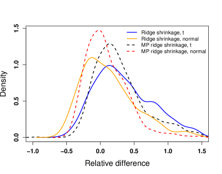
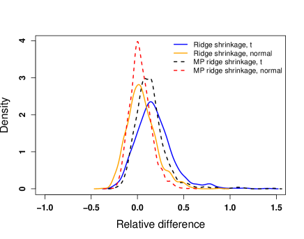
$\mathbf{c_{n}=2,\leavevmode\nobreak\ n=100}$	$\mathbf{c_{n}=2,\leavevmode\nobreak\ n=250}$
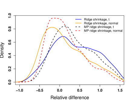
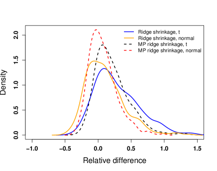
$\mathbf{c_{n}=4,\leavevmode\nobreak\ n=100}$	$\mathbf{c_{n}=4,\leavevmode\nobreak\ n=250}$

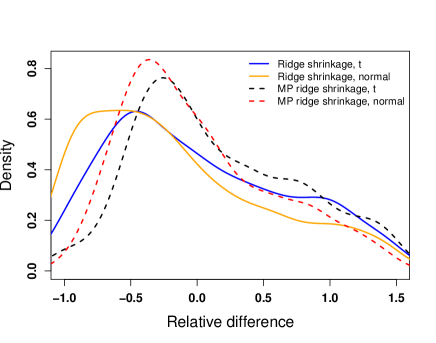
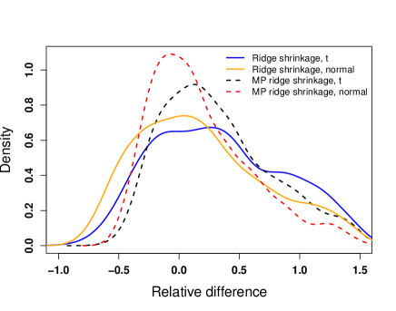
Figure 3: Relative differences of $t$’s that maximize $L^{2}_{R;n,2}(t)$ ($L^{2}_{MPR;n,2}(t)$) and $\hat{L}^{2}_{R;2}(t)$ ($\hat{L}^{2}_{MPR;2}(t)$) for $c_{n}\in\{1.1,2,4\}$, $n=100$ and $n=250$ when the elements of $\mathbf{X}_{n}$ are drawn from the normal distribution and scale $t$-distribution.

Figure 3 depicts the kernel density estimators of the relative differences between the values of $t$ which maximize $\hat{L}^{2}_{R;2}(t)$ and $L^{2}_{R;n,2}(t)$ in the case of the ridge estimator, and $L^{2}_{MPR;n,2}(t)$ and $\hat{L}^{2}_{MPR;2}(t)$ for the Moore-Penrose ridge estimator. The results are obtained when the elements of $\mathbf{X}_{n}$ are drawn from the normal distribution and $t$-distribution with $n\in\{100,250\}$ and $c_{n}\in\{1.1,2,4\}$. We observe that the computed kernel densities are concentrated around zero in almost all of the considered cases, except for the extreme case when $n=100$ and $c_{n}=4$. Furthermore, the kernel densities are skewed to the right with the exception when $n=250$ and $c_{n}=1.1$. As such, it can be concluded that the optimization of the estimated loss function instead of the true one may lead to larger values of the tuning parameter $t$. However, as the sample size increases, the difference between the two values, as expected, becomes negligible. Finally, faster convergence is achieved when the matrix $\mathbf{X}_{n}$ is drawn from the normal distribution.

Next, we compare the three suggested shrinkage approaches of Section 3 with the three benchmarks introduced at the beginning of this section. As a performance measure, we use the percentage relative improvement in average loss (PRIAL) defined by

$$\text{PRIAL}(\widehat{\bm{\Pi}})=\left(1-\dfrac{E||\widehat{\bm{\Pi}}\mathbf{\Sigma}-\mathbf{I}_{p}||^{2}_{F}}{E||\mathbf{S}_{n}^{+}\mathbf{\Sigma}-\mathbf{I}_{p}||_{F}^{2}}\right)\cdot 100\%\,,$$ (4.5)

where $\widehat{\bm{\Pi}}$ is an estimator of the precision matrix $\mathbf{\Sigma}^{-1}$. By definition, the PRIAL provides the percentage improvement of each strategy in comparison to the one based on the Moore-Penrose inverse. Moreover, it holds that PRIAL($\mathbf{\Sigma}^{-1}$)$=100\%$.

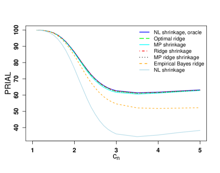
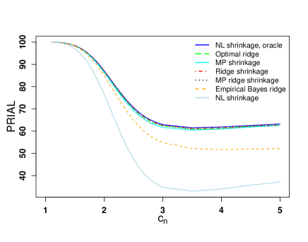
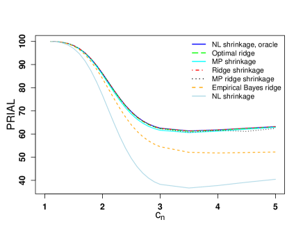
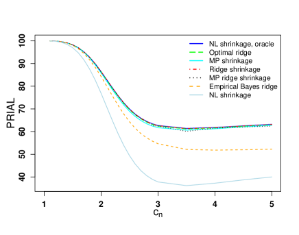
Figure 4: PRIAL for $c_{n}\in\{1.2,1.5,2,3.5,5\}$, $n=100$ (first row) and $n=250$ (second row) when the elements of $\mathbf{X}_{n}$ are drawn from the normal distribution (first column) and scale $t$-distribution (second column).

In Figure 4, we observe that the ridge shrinkage and the optimal ridge outperform the other estimators with the ridge shrinkage estimator having a slightly better performance. This observation holds for the two considered models of the data-generating process and for the selected values of $n$ and $c_{n}$. The Moore-Penrose shrinkage and the Moore-Penrose ridge shrinkage estimators are ranked in the third and fourth places with the Moore-Penrose ridge shrinkage estimator performing better in almost all cases with the exception of large values of $c_{n}$ when $n=250$. These two estimators are followed by the empirical Bayes ridge which performs better than the bona fide nonlinear shrinkage estimator. However, it has to be noted that the considered bona fide nonlinear shrinkage estimator was derived under the other loss function, which explains the considerable differences between the oracle and bona fide nonlinear shrinkage estimator. Finally, it is remarkable that both the ridge shrinkage and the optimal ridge attain the global benchmark, which is the oracle non-linear shrinkage estimator and as such, they can be considered optimal for the chosen data-generating models.

5 Summary

Although the Moore-Penrose inverse, the ridge inverse, and the Moore-Penrose ridge inverse of the sample covariance matrix are widely used in practice to estimate the precision matrix, their properties were derived under very restrictive assumptions in the literature, namely by assuming that a random sample is taken from the multivariate normal distribution and the true population covariance matrix is proportional to the diagonal matrix. When the population covariance matrix is not proportional to the diagonal matrix, then the first two moments of the Moore-Penrose inverse are characterized by some inequality constraints, derived under the assumption of normality.

We contribute to the existing literature by deriving the analytical expressions of the asymptotic behavior of the weighted sample trace moments of the three considered generalized inverse matrices. The results are obtained under the high-dimensional regime, i.e., when both the dimension of the data-generating model and the sample size tend to infinity without imposing any specific distributional assumption on the data-generating model. The obtained results are used to deduce improved estimators for the precision matrix. Within the extensive simulation study, it is documented that the new approaches outperform the existing methods.

6 Appendix

Proof of Theorem 2.1:.

Let $\mathbf{J}_{n}=\mathbf{I}_{n}-\frac{1}{n}\mathbf{1}_{n}\mathbf{1}_{n}^{\top}$. Then, $\mathbf{J}_{n}$ is a projection matrix of rank $n-1$. As such, all $n-1$ nonzero eigenvalues of $\mathbf{J}_{n}$ are equal to one, and its singular value decomposition is expressed as

$$\mathbf{J}_{n}=\mathbf{H}_{n}\mathbf{H}_{n}^{\top},$$

where $\mathbf{H}_{n}$ is a $n\times(n-1)$ orthogonal matrix, i.e., $\mathbf{H}_{n}^{\top}\mathbf{H}_{n}=\mathbf{I}_{n-1}$. Then,

$$\mathbf{S}_{n}=\frac{1}{n}\mathbf{Y}_{n}\mathbf{J}_{n}\mathbf{Y}_{n}^{\top}=\frac{1}{n}\widetilde{\mathbf{Y}}_{n}\widetilde{\mathbf{Y}}_{n}^{\top}\quad\text{with}\quad\widetilde{\mathbf{Y}}_{n}=\mathbf{H}_{n}\mathbf{Y}_{n}.$$ (6.1)

Moreover, since $\mathbf{H}_{n}$ is orthogonal and the rank of $\mathbf{Y}_{n}$ is equal to $n$, the application of Sylvester’s rank inequality leads to the conclusion that the rank of $\widetilde{\mathbf{Y}}_{n}$ is $n-1$ (see, Section 4.3.3 in Lütkepohl, (1996)). Hence, we get

$$\mathbf{S}_{n}^{+}=\left(\frac{1}{n}\widetilde{\mathbf{Y}}_{n}\widetilde{\mathbf{Y}}_{n}^{\top}\right)^{+}=\frac{1}{\sqrt{n}}\widetilde{\mathbf{Y}}_{n}\left(\frac{1}{n}\widetilde{\mathbf{Y}}_{n}^{\top}\widetilde{\mathbf{Y}}_{n}\right)^{-2}\frac{1}{\sqrt{n}}\widetilde{\mathbf{Y}}_{n}^{\top}$$ (6.2)

and, similarly,

$$(\mathbf{S}_{n}^{+})^{m}=\frac{1}{\sqrt{n}}\widetilde{\mathbf{Y}}_{n}\left(\frac{1}{n}\widetilde{\mathbf{Y}}_{n}^{\top}\widetilde{\mathbf{Y}}_{n}\right)^{-(m+1)}\frac{1}{\sqrt{n}}\widetilde{\mathbf{Y}}_{n}^{\top}\quad\text{for}\quad m=2,3,...$$ (6.3)

It holds that

$$\text{tr}\left[\frac{1}{\sqrt{n}}\widetilde{\mathbf{Y}}_{n}\left(\frac{1}{n}\widetilde{\mathbf{Y}}_{n}^{\top}\widetilde{\mathbf{Y}}_{n}\right)^{-(m+1)}\frac{1}{\sqrt{n}}\widetilde{\mathbf{Y}}_{n}^{\top}\mathbf{\Theta}\right]=\frac{(-1)^{m}}{m!}\left.\dfrac{\partial^{m}}{\partial t^{m}}\text{tr}\left[\frac{1}{\sqrt{n}}\widetilde{\mathbf{Y}}_{n}\left(\frac{1}{n}\widetilde{\mathbf{Y}}_{n}^{\top}\widetilde{\mathbf{Y}}_{n}+t\mathbf{I}_{n}\right)^{-1}\frac{1}{\sqrt{n}}\widetilde{\mathbf{Y}}_{n}^{\top}\mathbf{\Theta}\right]\right|_{t=0}$$

for $m=1,2,...$.

The application of the Woodbury formula (matrix inversion lemma, see, e.g., Horn and Johnsohn, (1985)), leads to

$$\frac{1}{\sqrt{n}}\widetilde{\mathbf{Y}}_{n}\left(\frac{1}{n}\widetilde{\mathbf{Y}}_{n}^{\top}\widetilde{\mathbf{Y}}_{n}+t\mathbf{I}_{n}\right)^{-1}\frac{1}{\sqrt{n}}\widetilde{\mathbf{Y}}_{n}^{\top}=\mathbf{I}_{p}-t\left(\frac{1}{n}\widetilde{\mathbf{Y}}_{n}\widetilde{\mathbf{Y}}_{n}^{\top}+t\mathbf{I}_{p}\right)^{-1}$$

$$= \mathbf{I}_{p}-t\mathbf{\Sigma}^{-1/2}\left(\frac{1}{n}\mathbf{X}_{n}\mathbf{X}_{n}^{\top}+t\mathbf{\Sigma}^{-1}-\bar{\mathbf{x}}_{n}\bar{\mathbf{x}}_{n}^{\top}\right)^{-1}\mathbf{\Sigma}^{-1/2},$$

where we use that

$$\frac{1}{n}\widetilde{\mathbf{Y}}_{n}\widetilde{\mathbf{Y}}_{n}^{\top}=\mathbf{S}_{n}=\frac{1}{n}\mathbf{\Sigma}^{1/2}\mathbf{X}_{n}\mathbf{X}_{n}^{\top}\mathbf{\Sigma}^{1/2}-\mathbf{\Sigma}^{1/2}\bar{\mathbf{x}}_{n}\bar{\mathbf{x}}_{n}^{\top}\mathbf{\Sigma}^{1/2}.$$

Hence,

$$\text{tr}((\mathbf{S}_{n}^{+})^{m}\mathbf{\Theta})=\frac{(-1)^{m+1}}{m!}\left.\dfrac{\partial^{m}}{\partial t^{m}}\,t\,\text{tr}\left[\left(\frac{1}{n}\mathbf{X}_{n}\mathbf{X}_{n}^{\top}+t\mathbf{\Sigma}^{-1}\right)^{-1}\mathbf{\Sigma}^{-1/2}\mathbf{\Theta}\mathbf{\Sigma}^{-1/2}\right]\right|_{t=0}$$

$$+ \frac{(-1)^{m+1}}{m!}\left.\dfrac{\partial^{m}}{\partial t^{m}}t\frac{\bar{\mathbf{x}}_{n}^{\top}\left(\frac{1}{n}\mathbf{X}_{n}\mathbf{X}_{n}^{\top}+t\mathbf{\Sigma}^{-1}\right)^{-1}\mathbf{\Sigma}^{-1/2}\mathbf{\Theta}\mathbf{\Sigma}^{-1/2}\left(\frac{1}{n}\mathbf{X}_{n}\mathbf{X}_{n}^{\top}+t\mathbf{\Sigma}^{-1}\right)^{-1}\bar{\mathbf{x}}_{n}}{1-\bar{\mathbf{x}}_{n}^{\top}\left(\frac{1}{n}\mathbf{X}_{n}\mathbf{X}_{n}^{\top}+t\mathbf{\Sigma}^{-1}\right)^{-1}\bar{\mathbf{x}}_{n}}\right|_{t=0}\,.$$

Following Pan, (2014, Eq. (2.28)), the quantity

$$\frac{1}{1-\bar{\mathbf{x}}_{n}^{\top}\left(\frac{1}{n}\mathbf{X}_{n}\mathbf{X}_{n}^{\top}+t\mathbf{\Sigma}^{-1}\right)^{-1}\bar{\mathbf{x}}_{n}}=\frac{1}{1-\bar{\mathbf{x}}_{n}^{\top}\mathbf{\Sigma}^{1/2}\left(\frac{1}{n}\mathbf{\Sigma}^{1/2}\mathbf{X}_{n}\mathbf{X}_{n}^{\top}\mathbf{\Sigma}^{1/2}+t\mathbf{I}_{p}\right)^{-1}\mathbf{\Sigma}^{1/2}\bar{\mathbf{x}}_{n}}$$

is uniformly bounded in $t$. Moreover, we have that

$$\left|\bm{\xi}^{\top}\left(\frac{1}{n}\mathbf{\Sigma}^{1/2}\mathbf{X}_{n}\mathbf{X}_{n}^{\top}\mathbf{\Sigma}^{1/2}+t\mathbf{I}_{n}\right)^{-1}\mathbf{\Sigma}^{1/2}\bar{\mathbf{x}}_{n}\right|\stackrel{{\scriptstyle a.s.}}{{\longrightarrow}}0$$ (6.4)

uniformly in $t$ following Pan, (2014, p. 673) where $\bm{\xi}^{\top}\bm{\xi}$ is assumed to be bounded. As a result, if $\mathbf{\Theta}=\sum_{i=1}^{k}\mbox{\boldmath$\theta$}_{i}\mbox{\boldmath$\theta$}_{i}^{\top}$ with finite $k$, then

$$\bar{\mathbf{x}}_{n}^{\top}\left(\frac{1}{n}\mathbf{X}_{n}\mathbf{X}_{n}^{\top}+t\mathbf{\Sigma}^{-1}\right)^{-1}\mathbf{\Sigma}^{-1/2}\mathbf{\Theta}\mathbf{\Sigma}^{-1/2}\left(\frac{1}{n}\mathbf{X}_{n}\mathbf{X}_{n}^{\top}+t\mathbf{\Sigma}^{-1}\right)^{-1}\bar{\mathbf{x}}_{n}$$

$$= \sum_{i=1}^{k}\left(\mbox{\boldmath$\theta$}_{i}^{\top}\mathbf{\Sigma}^{-1/2}\left(\frac{1}{n}\mathbf{X}_{n}\mathbf{X}_{n}^{\top}+t\mathbf{\Sigma}^{-1}\right)^{-1}\bar{\mathbf{x}}_{n}\right)^{2}$$

$$= \sum_{i=1}^{k}\left(\mbox{\boldmath$\theta$}_{i}^{\top}\left(\frac{1}{n}\mathbf{\Sigma}^{1/2}\mathbf{X}_{n}\mathbf{X}_{n}^{\top}\mathbf{\Sigma}^{1/2}+t\mathbf{I}_{n}\right)^{-1}\mathbf{\Sigma}^{1/2}\bar{\mathbf{x}}_{n}\right)^{2}\stackrel{{\scriptstyle a.s.}}{{\longrightarrow}}0$$

uniformly in $t$.

If the rank of $\mathbf{\Theta}$ is not finite and we assume that $\lambda_{max}(\mathbf{\Theta})=o(1)$, then we get

$$t\bar{\mathbf{x}}_{n}^{\top}\left(\frac{1}{n}\mathbf{X}_{n}\mathbf{X}_{n}^{\top}+t\mathbf{\Sigma}^{-1}\right)^{-1}\mathbf{\Sigma}^{-1/2}\mathbf{\Theta}\mathbf{\Sigma}^{-1/2}\left(\frac{1}{n}\mathbf{X}_{n}\mathbf{X}_{n}^{\top}+t\mathbf{\Sigma}^{-1}\right)^{-1}\bar{\mathbf{x}}_{n}$$

$$\leq \lambda_{max}\left(t\left(\frac{1}{n}\mathbf{X}_{n}\mathbf{X}_{n}^{\top}+t\mathbf{\Sigma}^{-1}\right)^{-1/2}\mathbf{\Sigma}^{-1/2}\mathbf{\Theta}\mathbf{\Sigma}^{-1/2}\left(\frac{1}{n}\mathbf{X}_{n}\mathbf{X}_{n}^{\top}+t\mathbf{\Sigma}^{-1}\right)^{-1/2}\right)$$

$$\times \bar{\mathbf{x}}_{n}^{\top}\left(\frac{1}{n}\mathbf{X}_{n}\mathbf{X}_{n}^{\top}+t\mathbf{\Sigma}^{-1}\right)^{-1}\bar{\mathbf{x}}_{n}$$

$$\leq \lambda_{max}\left(\mathbf{\Theta}\right)\lambda_{max}\left(t\mathbf{\Sigma}^{-1}\left(\frac{1}{n}\mathbf{X}_{n}\mathbf{X}_{n}^{\top}+t\mathbf{\Sigma}^{-1}\right)^{-1}\right)\bar{\mathbf{x}}_{n}^{\top}\left(\frac{1}{n}\mathbf{X}_{n}\mathbf{X}_{n}^{\top}+t\mathbf{\Sigma}^{-1}\right)^{-1}\bar{\mathbf{x}}_{n}$$

$$\leq \lambda_{max}\left(\mathbf{\Theta}\right)\bar{\mathbf{x}}_{n}^{\top}\left(\frac{1}{n}\mathbf{X}_{n}\mathbf{X}_{n}^{\top}+t\mathbf{\Sigma}^{-1}\right)^{-1}\bar{\mathbf{x}}_{n}\stackrel{{\scriptstyle a.s.}}{{\longrightarrow}}0$$

uniformly in $t$.

Thus,

$$\text{tr}((\mathbf{S}_{n}^{+})^{m}\mathbf{\Theta}) = \frac{(-1)^{m+1}}{m!}\left.\dfrac{\partial^{m}}{\partial t^{m}}\,t\,\text{tr}\left[\left(\frac{1}{n}\mathbf{X}_{n}\mathbf{X}_{n}^{\top}+t\mathbf{\Sigma}^{-1}\right)^{-1}\mathbf{\Sigma}^{-1/2}\mathbf{\Theta}\mathbf{\Sigma}^{-1/2}\right]\right|_{t=0}\,.$$

Lemma 6.2 in Bodnar et al., 2023b yields

$$\left|\text{tr}\left[\left(\frac{1}{n}\mathbf{X}_{n}\mathbf{X}_{n}^{\top}+t\mathbf{\Sigma}^{-1}\right)^{-1}\mathbf{\Sigma}^{-1/2}\mathbf{\Theta}\mathbf{\Sigma}^{-1/2}\right]-\text{tr}\left[\left(\tilde{v}(t)\mathbf{I}_{p}+t\mathbf{\Sigma}^{-1}\right)^{-1}\mathbf{\Sigma}^{-1/2}\mathbf{\Theta}\mathbf{\Sigma}^{-1/2}\right]\right|\stackrel{{\scriptstyle a.s.}}{{\rightarrow}}0,$$ (6.5)

for $p/n\rightarrow c\in[1,\infty)$ as $n\to\infty$ where $\tilde{v}(t)$ satisfies the following equation

$$\frac{1}{\tilde{v}(t)}-1=c_{n}\frac{1}{p}\text{tr}\left[\mathbf{\Sigma}\left(\tilde{v}(t)\mathbf{\Sigma}+t\mathbf{I}_{p}\right)^{-1}\right]$$

with $c_{n}=p/n$.

Let $v(t)=\tilde{v}(t)/t$. Then, $v(t)$ is the solution of the following equation

$$\frac{1}{v(t)}-t=c_{n}\frac{1}{p}\text{tr}\left[\mathbf{\Sigma}\left(v(t)\mathbf{\Sigma}+\mathbf{I}_{p}\right)^{-1}\right],$$ (6.6)

which can be rewritten as

$$1-tv(t)=c_{n}\frac{1}{p}\text{tr}\left[v(t)\mathbf{\Sigma}\left(v(t)\mathbf{\Sigma}+\mathbf{I}_{p}\right)^{-1}\right]=c_{n}-c_{n}\frac{1}{p}\text{tr}\left[\left(v(t)\mathbf{\Sigma}+\mathbf{I}_{p}\right)^{-1}\right],$$

As a result, $v(0)$ solves the equation

$$\frac{1}{p}\text{tr}\left[\left(v(0)\mathbf{\Sigma}+\mathbf{I}_{p}\right)^{-1}\right]=\frac{c_{n}-1}{c_{n}}.$$

The left hand-side of the equation is a monotonically decreasing function in $v(0)$ which the values from one to zero, while the right hand-side is equal to a number smaller than one. As a result, there is a unique solution of this equation, which is bounded for the fixed value of $c_{n}$.

Let

$$f_{1}(v)=\frac{1}{v}\quad\text{and}\quad f_{2}(v;\mbox{\boldmath$A$})=\frac{1}{p}\text{tr}\left[\left(v\mathbf{I}_{p}+\mathbf{\Sigma}^{-1}\right)^{-1}\mbox{\boldmath$A$}\right].$$ (6.7)

for a matrix $A$. Then, the $k$-th order derivatives of these two functions are expressed as

$$f_{1}^{(k)}(v)=(-1)^{k}k!\frac{1}{v^{k+1}}$$

and

$$f_{2}^{(k)}(v;\mbox{\boldmath$A$}) = \frac{(-1)^{k}k!}{p}\text{tr}\left[\left(v\mathbf{I}_{p}+\mathbf{\Sigma}^{-1}\right)^{-(k+1)}\mbox{\boldmath$A$}\right]$$

$$= \frac{(-1)^{k}k!}{p}\text{tr}\left\{\left(v\mathbf{\Sigma}+\mathbf{I}_{p}\right)^{-1}\left[\mathbf{\Sigma}\left(v\mathbf{\Sigma}+\mathbf{I}_{p}\right)^{-1}\right]^{k}\mathbf{\Sigma}^{1/2}\mbox{\boldmath$A$}\mathbf{\Sigma}^{1/2}\right\}$$

for $k=1,2,...$. Then, the application of the Faà di Bruno formula (see, Section 1.3 in Krantz and Parks, (2002)) leads to

$$\text{tr}((\mathbf{S}_{n}^{+})^{m}\mathbf{\Theta})\stackrel{{\scriptstyle a.s.}}{{\longrightarrow}}\frac{(-1)^{m+1}}{m!}\left.\dfrac{\partial^{m}}{\partial t^{m}}\,t\,\text{tr}\left[\left(\tilde{v}(t)\mathbf{I}_{p}+t\mathbf{\Sigma}^{-1}\right)^{-1}\mathbf{\Sigma}^{-1/2}\mathbf{\Theta}\mathbf{\Sigma}^{-1/2}\right]\right|_{t=0}$$

$$= \frac{(-1)^{m+1}}{m!}\left.\dfrac{\partial^{m}}{\partial t^{m}}\text{tr}\left[\left(v(t)\mathbf{I}_{p}+\mathbf{\Sigma}^{-1}\right)^{-1}\mathbf{\Sigma}^{-1/2}\mathbf{\Theta}\mathbf{\Sigma}^{-1/2}\right]\right|_{t=0}$$

$$= \frac{(-1)^{m+1}}{m!}\sum_{k=1}^{m}f_{2}^{(k)}(v(0);\mathbf{\Sigma}^{-1/2}\mathbf{\Theta}\mathbf{\Sigma}^{-1/2})B_{m,k}\left(v^{\prime}(0),v^{\prime\prime}(0),...,v^{(m-k+1)}(0)\right)$$

$$= \sum_{k=1}^{m}\frac{(-1)^{m+k+1}k!}{m!p}\text{tr}\left\{\left(v(0)\mathbf{\Sigma}+\mathbf{I}_{p}\right)^{-1}\left[\mathbf{\Sigma}\left(v(0)\mathbf{\Sigma}+\mathbf{I}_{p}\right)^{-1}\right]^{k}\mathbf{\Theta}\right\}B_{m,k}\left(v^{\prime}(0),v^{\prime\prime}(0),...,v^{(m-k+1)}(0)\right)$$

for $p/n\rightarrow c\in(1,\infty)$ as $n\rightarrow\infty$ where the symbol $B_{m,k}\left(v_{1},v_{2},...,v_{m-k+1}\right)$ denotes the partial exponential Bell polynomials defined in the statement of the theorem.

To compute $v^{\prime}(0)$, $v^{\prime\prime}(0)$,…,$v^{(m-k+1)}(0)$, we rewrite (6.6) as

$$\frac{1}{v(t)}-t=c_{n}\frac{1}{p}\text{tr}\left[\left(v(t)\mathbf{I}_{p}+\mathbf{\Sigma}^{-1}\right)^{-1}\right].$$ (6.8)

Hence,

$$-\frac{v^{\prime}(t)}{v(t)^{2}}-1=-c_{n}v^{\prime}(t)\frac{1}{p}\text{tr}\left[\left(v(t)\mathbf{I}_{p}+\mathbf{\Sigma}^{-1}\right)^{-2}\right]=-c_{n}v^{\prime}(t)\frac{1}{p}\text{tr}\left\{\left[\mathbf{\Sigma}\left(v(t)\mathbf{\Sigma}+\mathbf{I}_{p}\right)^{-1}\right]^{2}\right\},$$

from which we get

$$v^{\prime}(0) = -\frac{1}{\frac{1}{v(0)^{2}}-c_{n}\frac{1}{p}\text{tr}\left\{\left[\mathbf{\Sigma}\left(v(0)\mathbf{\Sigma}+\mathbf{I}_{p}\right)^{-1}\right]^{2}\right\}}$$

For the computation of the derivative of $v(.)$ of the order larger than one, we apply the Faà di Bruno formula to both the sides of (6.8). This yields

$$\sum_{k=1}^{m}f_{1}^{(k)}(v(t))B_{m,k}\left(v^{\prime}(t),...,v^{(m-k+1)}(t)\right)=c_{n}\sum_{k=1}^{m}f_{2}^{(k)}(v(t);\mathbf{I}_{p})B_{m,k}\left(v^{\prime}(t),...,v^{(m-k+1)}(t)\right)$$

or

$$\sum_{k=1}^{m}\frac{(-1)^{k}k!}{v(t)^{k+1}}B_{m,k}\left(v^{\prime}(t),...,v^{(m-k+1)}(t)\right)$$

$$= c_{n}\sum_{k=1}^{m}\frac{(-1)^{k}k!}{p}\text{tr}\left\{\left[\mathbf{\Sigma}\left(v(t)\mathbf{\Sigma}+\mathbf{I}_{p}\right)^{-1}\right]^{k+1}\right\}B_{m,k}\left(v^{\prime}(t),...,v^{(m-k+1)}(t)\right)$$

Using that $B_{m,1}\left(v^{\prime}(t),v^{\prime\prime}(t),...,v^{(m)}(t)\right)=v^{(m)}(t)$, we finally get

$$v^{(m)}(0)=\frac{\sum_{k=2}^{m}(-1)^{k}k!\left(\frac{1}{v(0)^{k+1}}-c_{n}\frac{1}{p}\text{tr}\left\{\left[\mathbf{\Sigma}\left(v(0)\mathbf{\Sigma}+\mathbf{I}_{p}\right)^{-1}\right]^{k+1}\right\}\right)B_{m,k}\left(v^{\prime}(0),...,v^{(m-k+1)}(0)\right)}{\frac{1}{v(0)^{2}}-c_{n}\frac{1}{p}\text{tr}\left\{\left[\mathbf{\Sigma}\left(v(0)\mathbf{\Sigma}+\mathbf{I}_{p}\right)^{-1}\right]^{2}\right\}}$$

∎

Proof of Corollary 2.2:.

Let

$$g_{k}=\frac{1}{p}\text{tr}\left\{\left[\mathbf{\Sigma}\left(v(0)\mathbf{\Sigma}+\mathbf{I}_{p}\right)^{-1}\right]^{k}\right\}.$$

Then,

$$d_{k}\left(\frac{1}{p}\mathbf{I}_{p}\right)=\frac{1}{p}\text{tr}\left\{\left(v(0)\mathbf{\Sigma}+\mathbf{I}_{p}\right)^{-1}\left[\mathbf{\Sigma}\left(v(0)\mathbf{\Sigma}+\mathbf{I}_{p}\right)^{-1}\right]^{k}\mathbf{I}_{p}\right\}=g_{k}-v(0)g_{k+1}$$

and, consequently,

$$s_{m}\left(\frac{1}{p}\mathbf{I}_{p}\right) = \sum_{k=1}^{m}\frac{(-1)^{m+k+1}k!}{m!}\left(g_{k}-v(0)g_{k+1}\right)B_{m,k}\left(v^{\prime}(0),...,v^{(m-k+1)}(0)\right)$$

$$= \frac{(-1)^{m}}{m!}\left(g_{1}-v(0)g_{2}\right)B_{m,1}\left(v^{\prime}(0),...,v^{(m)}(0)\right)$$

$$+ \sum_{k=2}^{m}\frac{(-1)^{m+k+1}k!}{m!}\left(g_{k}-v(0)g_{k+1}\right)B_{m,k}\left(v^{\prime}(0),...,v^{(m-k+1)}(0)\right).$$

The application of $B_{m,1}\left(v^{\prime}(0),...,v^{(m)}(0)\right)=v^{(m)}(0)$ and (2.9) yields

$$s_{m}\left(\frac{1}{p}\mathbf{I}_{p}\right)=\frac{(-1)^{m+1}}{m!}\sum_{k=2}^{m}(-1)^{k}k!\left(g_{1}-v(0)g_{2}\right)v^{\prime}(0)h_{k+1}B_{m,k}\left(v^{\prime}(0),...,v^{(m-k+1)}(0)\right)$$

$$+ \frac{(-1)^{m+1}}{m!}\sum_{k=2}^{m}(-1)^{k}k!\left(g_{k}-v(0)g_{k+1}\right)B_{m,k}\left(v^{\prime}(0),...,v^{(m-k+1)}(0)\right)$$

$$= \frac{(-1)^{m+1}}{m!}\sum_{k=2}^{m}(-1)^{k}k!\left[\left(g_{1}-v(0)g_{2}\right)v^{\prime}(0)h_{k+1}+g_{k}-v(0)g_{k+1}\right]B_{m,k}\left(v^{\prime}(0),...,v^{(m-k+1)}(0)\right).$$

Using

$$\left(g_{1}-v(0)g_{2}\right)v^{\prime}(0)h_{k+1}+g_{k}-v(0)g_{k+1}$$

$$= \left(\frac{1}{p}\text{tr}\left[\mathbf{\Sigma}\left(v(0)\mathbf{\Sigma}+\mathbf{I}_{p}\right)^{-1}\right]-v(0)g_{2}\right)\frac{-v(0)^{2}}{1-c_{n}v(0)^{2}g_{2}}h_{k+1}+g_{k}-v(0)g_{k+1}$$

$$= \left(\frac{1}{v(0)}\left(1-\frac{1}{p}\text{tr}\left[\left(v(0)\mathbf{\Sigma}+\mathbf{I}_{p}\right)^{-1}\right]\right)-v(0)g_{2}\right)\frac{-v(0)^{2}}{1-c_{n}v(0)^{2}g_{2}}h_{k+1}+g_{k}-v(0)g_{k+1}$$

$$= \left(\frac{1}{v(0)}\left(1-\frac{c_{n}}{c_{n}-1}\right)-v(0)g_{2}\right)\frac{-v(0)^{2}}{1-c_{n}v(0)^{2}g_{2}}h_{k+1}+g_{k}-v(0)g_{k+1}$$

$$= \frac{-v(0)}{c_{n}}h_{k+1}+g_{k}-v(0)g_{k+1}=\frac{-h_{k}}{c_{n}}$$

and the equality (see, Equation (1.4) in Cvijović, (2011))

$$k!B_{m,k}\left(v^{\prime}(0),...,v^{(m-k+1)}(0)\right)=(k-1)!\sum_{r=1}^{m-1}\frac{m!}{r!(m-r)!}v^{(r)}(0)B_{m-r,k-1}\left(v^{\prime}(0),...,v^{(m-r-k+2)}(0)\right),$$

where $B_{i,k-1}(.)=0$ for $i<k-1$, we get

$$s_{m}\left(\frac{1}{p}\mathbf{I}_{p}\right) = \frac{(-1)^{m}}{m!c_{n}}\sum_{k=2}^{m}(-1)^{k}h_{k}(k-1)!\sum_{r=1}^{m-1}\frac{m!}{r!(m-r)!}v^{(r)}(0)B_{m-r,k-1}\left(v^{\prime}(0),...,v^{(m-r-k)}(0)\right)$$

$$= \frac{(-1)^{m}}{m!c_{n}}\sum_{r=1}^{m-1}\frac{m!}{r!(m-r)!}v^{(r)}(0)\sum_{k=2}^{m-r+1}(-1)^{k}h_{k}(k-1)!B_{m-r,k-1}\left(v^{\prime}(0),...,v^{(m-r-k+2)}(0)\right)$$

$$= \frac{(-1)^{m}}{m!c_{n}}\frac{m!}{(m-1)!}v^{(m-1)}(0)h_{2}v^{\prime}(0)+\frac{(-1)^{m}}{m!c_{n}}\sum_{r=1}^{m-2}\frac{m!}{r!(m-r)!}v^{(r)}(0)\Bigg{(}h_{2}v^{(m-r)}(0)$$

$$- \sum_{k=3}^{m-r+1}(-1)^{k-1}h_{k}(k-1)!B_{m-r,k-1}\left(v^{\prime}(0),...,v^{(m-r-k+2)}(0)\right)\Bigg{)}$$

$$= \frac{(-1)^{m-1}}{(m-1)!c_{n}}v^{(m-1)}(0),$$

where we used that $v^{\prime}(0)=-h_{2}^{-1}$ and

$$\sum_{k=3}^{m-r+1}(-1)^{k-1}h_{k}(k-1)!B_{m-r,k-1}\left(v^{\prime}(0),...,v^{(m-r-k+2)}(0)\right)\Bigg{)}=-\frac{v^{(m-r)}(0)}{v^{\prime}(0)}.$$

∎

Proof of Corollary 2.3:.

From the proof of Theorem 2.1 we deduce that

$$B_{1,1}\left(v^{\prime}(0)\right)=v^{\prime}(0),\;B_{2,1}\left(v^{\prime}(0),v^{\prime\prime}(0)\right)=v^{\prime\prime}(0),\;$$

$$B_{3,1}\left(v^{\prime}(0),v^{\prime\prime}(0),v^{\prime\prime\prime}(0)\right)=v^{\prime\prime\prime}(0),\;B_{4,1}\left(v^{\prime}(0),v^{\prime\prime}(0),v^{\prime\prime\prime}(0),v^{\prime\prime\prime\prime}(0)\right)=v^{\prime\prime\prime\prime}(0).$$

Furthermore, it holds that

$$B_{2,2}\left(v^{\prime}(0)\right) = [v^{\prime}(0)]^{2},$$

$$B_{3,2}\left(v^{\prime}(0),v^{\prime\prime}(0)\right) = 3v^{\prime}(0)v^{\prime\prime}(0),$$

$$B_{3,3}\left(v^{\prime}(0)\right) = [v^{\prime}(0)]^{3},$$

$$B_{4,2}\left(v^{\prime}(0),v^{\prime\prime}(0),v^{\prime\prime\prime}(0)\right) = 4v^{\prime}(0)v^{\prime\prime\prime}(0)+3[v^{\prime\prime}(0)]^{2},$$

$$B_{4,3}\left(v^{\prime}(0),v^{\prime\prime}(0)\right) = 6[v^{\prime}(0)]^{2}v^{\prime\prime}(0),$$

$$B_{4,4}\left(v^{\prime}(0)\right) = [v^{\prime}(0)]^{4}.$$

The substitution of the computed formulas for the partial exponential Bell polynomials to (2.5) and (2.9) and the application of (2.8) yield the statement of the corollary. ∎

Proof of Corollary 2.4:.

If $\mathbf{\Sigma}=\mathbf{I}_{p}$, then

$$d_{k}\left(\mathbf{\Theta}\right)=\left(v(0)+1\right)^{-(k+1)}\text{tr}(\mathbf{\Theta}),\quad k=1,2,....$$

and $s_{m}(\mathbf{\Theta})=a_{m}\text{tr}(\mathbf{\Theta})$ for $m=1,2,...$ where $a_{m}$ does not depend on $\mathbf{\Theta}$. As such, $a_{m}$ can be computed by setting $\mathbf{\Theta}=\frac{1}{p}\mathbf{I}_{p}$ and using the findings of Corollary 2.2. Thus,

$$s_{m}\left(\mathbf{\Theta}\right)=s_{m}\left(\frac{1}{p}\mathbf{I}_{p}\right)\text{tr}(\mathbf{\Theta})=\frac{(-1)^{m-1}v^{(m-1)}(0)}{(m-1)!c_{n}}\text{tr}(\mathbf{\Theta}),$$

where it holds from (2.7) that

$$\frac{1}{v(0)+1}=\frac{c_{n}-1}{c_{n}}$$

and, hence,

$$v(0)=\frac{1}{c_{n}-1}\quad\text{and}\quad v^{\prime}(0)=-\frac{c_{n}}{(c_{n}-1)^{3}},$$ (6.9)

where the second equality follows from (2.8).

Finally, from (2.9) we get

$$v^{(m)}(0) = -v^{\prime}(0)\sum_{k=2}^{m}(-1)^{k}k!\left(v(0)^{-(k+1)}-c_{n}(v(0)+1)^{-(k+1)}\right)B_{m,k}\left(v^{\prime}(0),...,v^{(m-k+1)}(0)\right)$$

$$= \frac{c_{n}}{(c_{n}-1)^{3}}\sum_{k=2}^{m}(-1)^{k}k!(c_{n}-1)^{(k+1)}\left(1-c_{n}^{-k}\right)B_{m,k}\left(v^{\prime}(0),...,v^{(m-k+1)}(0)\right).$$

∎

Proof of Theorem 2.5:.

Following the proof of Theorem 2.1 we get

$$\text{tr}((\mathbf{S}_{n}+t\mathbf{I}_{p})^{-(m+1)}\mathbf{\Theta}) = \frac{(-1)^{m}}{m!}\dfrac{\partial^{m}}{\partial t^{m}}\,\text{tr}\left[\left(\frac{1}{n}\mathbf{X}_{n}\mathbf{X}_{n}^{\top}+t\mathbf{\Sigma}^{-1}\right)^{-1}\mathbf{\Sigma}^{-1/2}\mathbf{\Theta}\mathbf{\Sigma}^{-1/2}\right]\,,$$

while the application of Lemma 6.2 in Bodnar et al., 2023b leads to

$$\left|\text{tr}\left[\left(\frac{1}{n}\mathbf{X}_{n}\mathbf{X}_{n}^{\top}+t\mathbf{\Sigma}^{-1}\right)^{-1}\mathbf{\Sigma}^{-1/2}\mathbf{\Theta}\mathbf{\Sigma}^{-1/2}\right]-\frac{1}{t}\text{tr}\left[\left(v(t)\mathbf{I}_{p}+\mathbf{\Sigma}^{-1}\right)^{-1}\mathbf{\Sigma}^{-1/2}\mathbf{\Theta}\mathbf{\Sigma}^{-1/2}\right]\right|\stackrel{{\scriptstyle a.s.}}{{\rightarrow}}0,$$ (6.10)

for $p/n\rightarrow c\in[1,\infty)$ as $n\to\infty$ where $v(t)$ is the solution of (6.6). Hence,

$$\text{tr}((\mathbf{S}_{n}+t\mathbf{I}_{p})^{-(m+1)}\mathbf{\Theta})\stackrel{{\scriptstyle a.s.}}{{\longrightarrow}}\frac{(-1)^{m}}{m!}\dfrac{\partial^{m}}{\partial t^{m}}\frac{1}{t}\text{tr}\left[\left(v(t)\mathbf{I}_{p}+\mathbf{\Sigma}^{-1}\right)^{-1}\mathbf{\Sigma}^{-1/2}\mathbf{\Theta}\mathbf{\Sigma}^{-1/2}\right]$$

$$= \frac{(-1)^{m}}{m!}\dfrac{\partial^{m}{1}/{t}}{\partial t^{m}}\text{tr}\left[\left(v(t)\mathbf{I}_{p}+\mathbf{\Sigma}^{-1}\right)^{-1}\mathbf{\Sigma}^{-1/2}\mathbf{\Theta}\mathbf{\Sigma}^{-1/2}\right]$$

$$+\frac{(-1)^{m}}{m!}\sum_{l=1}^{m}\frac{m!}{l!(m-l)!}\dfrac{\partial^{m-l}}{\partial t^{m-l}}\frac{1}{t}\dfrac{\partial^{l}}{\partial t^{l}}\text{tr}\left[\left(v(t)\mathbf{I}_{p}+\mathbf{\Sigma}^{-1}\right)^{-1}\mathbf{\Sigma}^{-1/2}\mathbf{\Theta}\mathbf{\Sigma}^{-1/2}\right]$$

$$= t^{-m-1}\text{tr}\left[\left(v(t)\mathbf{I}_{p}+\mathbf{\Sigma}^{-1}\right)^{-1}\mathbf{\Sigma}^{-1/2}\mathbf{\Theta}\mathbf{\Sigma}^{-1/2}\right]$$

$$+\frac{(-1)^{m}}{m!}\sum_{l=1}^{m}\frac{m!}{l!(m-l)!}(-1)^{m-l}(m-l)!t^{-(m-l)-1}\sum_{k=1}^{l}f_{2}^{(k)}(v(t);\mathbf{\Sigma}^{-1/2}\mathbf{\Theta}\mathbf{\Sigma}^{-1/2})$$

$$\times B_{l,k}\left(v^{\prime}(t),v^{\prime\prime}(t),...,v^{(l-k+1)}(t)\right)$$

$$= t^{-m-1}\text{tr}\left[\left(v(t)\mathbf{\Sigma}+\mathbf{I}_{p}\right)^{-1}\mathbf{\Theta}\right]$$

$$+\sum_{l=1}^{m}t^{-(m-l)-1}\sum_{k=1}^{l}\frac{(-1)^{l+k}k!}{l!}\text{tr}\left\{\left(v(t)\mathbf{\Sigma}+\mathbf{I}_{p}\right)^{-1}\left[\mathbf{\Sigma}\left(v(t)\mathbf{\Sigma}+\mathbf{I}_{p}\right)^{-1}\right]^{k}\mathbf{\Theta}\right\}$$

$$\times B_{l,k}\left(v^{\prime}(t),v^{\prime\prime}(t),...,v^{(l-k+1)}(t)\right)$$

for $p/n\rightarrow c\in(1,\infty)$ as $n\rightarrow\infty$. Furthermore, $v(t)$ is the solution of (6.6) which can be rewritten as (2.21),

$$v^{\prime}(t) = -\frac{1}{\frac{1}{v(t)^{2}}-c_{n}\frac{1}{p}\text{tr}\left\{\left[\mathbf{\Sigma}\left(v(t)\mathbf{\Sigma}+\mathbf{I}_{p}\right)^{-1}\right]^{2}\right\}},$$

and

$$v^{(m)}(t)=\frac{\sum_{k=2}^{m}(-1)^{k}k!\left(\frac{1}{v(t)^{k+1}}-c_{n}\frac{1}{p}\text{tr}\left\{\left[\mathbf{\Sigma}\left(v(t)\mathbf{\Sigma}+\mathbf{I}_{p}\right)^{-1}\right]^{k+1}\right\}\right)B_{m,k}\left(v^{\prime}(t),...,v^{(m-k+1)}(t)\right)}{\frac{1}{v(t)^{2}}-c_{n}\frac{1}{p}\text{tr}\left\{\left[\mathbf{\Sigma}\left(v(t)\mathbf{\Sigma}+\mathbf{I}_{p}\right)^{-1}\right]^{2}\right\}}.$$

∎

Proof of Corollary 2.6:.

The proof of Corollary 2.6 is done by using the methods of mathematical induction. For $m=0$, we get

$$\tilde{s}_{1}\left(t,\frac{1}{p}\mathbf{I}_{p}\right)=t^{-1}d_{k}\left(t,\frac{1}{p}\mathbf{I}_{p}\right)=t^{-1}\frac{c_{n}-1}{c_{n}}+\frac{v(t)}{c_{n}},$$

where the last equality follows from (2.21) and 2.20.

Next, we assume that the statement of the corollary is true for $\tilde{s}_{1}\left(t,\frac{1}{p}\mathbf{I}_{p}\right),...\tilde{s}_{m}\left(t,\frac{1}{p}\mathbf{I}_{p}\right)$ and prove it for $\tilde{s}_{m+1}\left(t,\frac{1}{p}\mathbf{I}_{p}\right)$. Let

$$g_{k}(t)=\frac{1}{p}\text{tr}\left\{\left[\mathbf{\Sigma}\left(v(t)\mathbf{\Sigma}+\mathbf{I}_{p}\right)^{-1}\right]^{k}\right\}.$$

Then,

$$d_{k}\left(t,\frac{1}{p}\mathbf{I}_{p}\right)=\frac{1}{p}\text{tr}\left\{\left(v(t)\mathbf{\Sigma}+\mathbf{I}_{p}\right)^{-1}\left[\mathbf{\Sigma}\left(v(t)\mathbf{\Sigma}+\mathbf{I}_{p}\right)^{-1}\right]^{k}\mathbf{I}_{p}\right\}=g_{k}(t)-v(t)g_{k+1}(t)$$

and $h_{k}(t)=v(t)^{-k}-c_{n}g_{k}(t)$. Moreover, from the definition of $v^{\prime}(t)$ we have

$$v^{\prime}(t)h_{2}(t)=-1$$

and

$$v^{\prime}(t)(g_{1}(t)-v(t)g_{2}(t))=\frac{-1}{v(t)^{-2}-c_{n}g_{2}(t)}\left(\frac{1-tv(t)}{c_{n}v(t)}-v(t)g_{2}(t)\right)=-\frac{v(t)}{c_{n}}-\frac{tv^{\prime}(t)}{c_{n}}.$$

Using the recursion (2.25) and the assumption of the induction, we get

$$\tilde{s}_{m+1}\left(t,\frac{1}{p}\mathbf{I}_{p}\right) = t^{-(m+1)}\frac{c_{n}-1}{c_{n}}+t^{-1}\frac{(-1)^{m-1}v^{(m-1)}(t)}{(m-1)!c_{n}}$$

$$+ t^{-1}\Bigg{(}\frac{(-1)^{m-1}}{m!}\left(g_{1}(t)-v(t)g_{2}(t)\right)B_{m,1}\left(v^{\prime}(t),...,v^{(m)}(t)\right)$$

$$+ \sum_{k=2}^{m}\frac{(-1)^{m+k}k!}{m!}\left(g_{k}(t)-v(t)g_{k+1}(t)\right)B_{m,k}\left(v^{\prime}(t),...,v^{(m-k+1)}(t)\right)\Bigg{)}$$

$$= t^{-(m+1)}\frac{c_{n}-1}{c_{n}}+t^{-1}\frac{(-1)^{m-1}v^{(m-1)}(t)}{(m-1)!c_{n}}$$

$$+ \frac{(-1)^{m}}{m!t}\sum_{k=2}^{m}(-1)^{k}k!\left[\left(g_{1}(t)-v(t)g_{2}(t)\right)v^{\prime}(t)h_{k+1}(t)+g_{k}(t)-v(t)g_{k+1}(t)\right]$$

$$\times B_{m,k}\left(v^{\prime}(t),...,v^{(m-k+1)}(t)\right),$$

following the proof of Corollary 2.2 where

$$\left(g_{1}(t)-v(t)g_{2}(t)\right)v^{\prime}(t)h_{k+1}(t)+g_{k}(t)-v(t)g_{k+1}(t)$$

$$= \left(-\frac{v(t)}{c_{n}}-\frac{tv^{\prime}(t)}{c_{n}}\right)h_{k+1}(t)+g_{k}(t)-v(t)g_{k+1}(t)=-\frac{h_{k}(t)}{c_{n}}-\frac{tv^{\prime}(t)}{c_{n}}h_{k+1}(t).$$

Hence,

$$\tilde{s}_{m+1}\left(t,\frac{1}{p}\mathbf{I}_{p}\right) = t^{-(m+1)}\frac{c_{n}-1}{c_{n}}+t^{-1}\frac{(-1)^{m-1}v^{(m-1)}(t)}{(m-1)!c_{n}}$$

$$+ t^{-1}\frac{(-1)^{m-1}}{m!c_{n}}\sum_{k=2}^{m}(-1)^{k}k!h_{k}(t)B_{m,k}\left(v^{\prime}(t),...,v^{(m-k+1)}(t)\right)$$

$$+ \frac{(-1)^{m}}{m!c_{n}}(-1)v^{\prime}(t)\sum_{k=2}^{m}(-1)^{k}k!h_{k+1}(t)B_{m,k}\left(v^{\prime}(t),...,v^{(m-k+1)}(t)\right)$$

$$= t^{-(m+1)}\frac{c_{n}-1}{c_{n}}+t^{-1}\frac{(-1)^{m}v^{(m)}(t)}{m!c_{n}},$$

following the end of the proof of Corollary 2.2. ∎

Proof of Theorem 2.7:.

Let $t_{1}<t_{2}$. The application of (2.21) yields

$$\frac{1}{p}\text{tr}\left[\left(v(t_{1})\mathbf{\Sigma}+\mathbf{I}_{p}\right)^{-1}\right]-\frac{1}{p}\text{tr}\left[\left(v(t_{2})\mathbf{\Sigma}+\mathbf{I}_{p}\right)^{-1}\right]=\frac{t_{1}v(t_{1})-t_{2}v(t_{2})}{c_{n}}.$$ (6.11)

Assume that the statement of the theorem is wrong for the considered $t_{1}$ and $t_{2}$, i.e., $v(t_{1})\leq v(t_{2})$. Then, the left hand-side of (6.11) is nonnegative. On the other side the right hand-side of (6.11) is nonnegative only if

$$\frac{t_{1}}{t_{2}}\geq\frac{v(t_{2})}{v(t_{1})},$$

which contradicts that $v(t_{1})\leq v(t_{2})$. The theorem is proved. ∎

Proof of Corollary 2.8:.

The application of Theorem 2.5 leads to

$$\tilde{s}_{1}(t,\mathbf{\Theta})=t^{-1}d_{0}(t,\mathbf{\Theta}),$$

$$\tilde{s}_{2}(t,\mathbf{\Theta})=t^{-2}d_{0}(t,\mathbf{\Theta})+t^{-1}d_{1}(t,\mathbf{\Theta})B_{1,1}\left(v^{\prime}(t)\right),$$

$$\tilde{s}_{3}(t,\mathbf{\Theta})=t^{-3}d_{0}(t,\mathbf{\Theta})+t^{-2}d_{1}(t,\mathbf{\Theta})B_{1,1}\left(v^{\prime}(t)\right)$$

$$+t^{-1}\left\{-\frac{1}{2}v^{\prime\prime}(t)d_{1}(t,\mathbf{\Theta})B_{2,1}\left(v^{\prime}(t),v^{\prime\prime}(t)\right)+d_{2}(t,\mathbf{\Theta})B_{2,2}\left(v^{\prime}(t)\right)\right\},$$

$$\tilde{s}_{4}(t,\mathbf{\Theta})=t^{-4}d_{0}(t,\mathbf{\Theta})+t^{-3}d_{1}(t,\mathbf{\Theta})B_{3,1}\left(v^{\prime}(t)\right)$$

$$+t^{-2}\left\{-\frac{1}{2}d_{1}(t,\mathbf{\Theta})B_{2,1}\left(v^{\prime}(t),v^{\prime\prime}(t)\right)+d_{2}(t,\mathbf{\Theta})B_{2,2}\left(v^{\prime}(t)\right)\right\}$$

$$+t^{-1}\left\{\frac{1}{6}d_{1}(t,\mathbf{\Theta})B_{3,1}\left(v^{\prime}(t),v^{\prime\prime}(t)v^{\prime\prime\prime}(t)\right)-\frac{1}{3}d_{2}(t,\mathbf{\Theta})B_{3,2}\left(v^{\prime}(t),v^{\prime\prime}(t)\right)+d_{3}(t,\mathbf{\Theta})B_{3,3}\left(v^{\prime}(t)\right)\right\}.$$

The rest of the proof follows by using the formulas for the partial exponential Bell polynomials as given in the proof of Corollary 2.3.

∎

Proof of Corollary 2.9:.

If $\mathbf{\Sigma}=\mathbf{I}_{p}$, then

$$d_{k}\left(t,\mathbf{\Theta}\right)=\left(v(t)+1\right)^{-(k+1)}\text{tr}(\mathbf{\Theta}),\quad k=0,1,2,....$$

As a result, $\tilde{s}_{m+1}(t,\mathbf{\Theta})=a_{m+1}(t)\text{tr}(\mathbf{\Theta})$ for $m=0,1,...$ where $a_{m+1}(t)$, $m=0,1,...$, does not depend on $\mathbf{\Theta}$. Consequently, $a_{m+1}(t)$, $m=0,1,...$, can be computed by setting $\mathbf{\Theta}=\frac{1}{p}\mathbf{I}_{p}$ and using the results of Corollary 2.6. It leads to

$$\tilde{s}_{m+1}\left(t,\mathbf{\Theta}\right)=\tilde{s}_{m+1}\left(t,\frac{1}{p}\mathbf{I}_{p}\right)\text{tr}(\mathbf{\Theta})=\left(t^{-(m+1)}\frac{c_{n}-1}{c_{n}}+\frac{(-1)^{m}v^{(m)}(t)}{(m)!c_{n}}\right)\text{tr}(\mathbf{\Theta}),$$

where $v(t)$ is the solution of

$$\frac{1}{v(t)+1}=\frac{c_{n}-1+tv(t)}{c_{n}}$$

and, hence,

$$v(t)=\frac{-(c_{n}-1+t)+\sqrt{(c_{n}-1+t)^{2}+4t}}{2t}=\frac{2}{(c_{n}-1+t)+\sqrt{(c_{n}-1+t)^{2}+4t}}.$$

Moreover, it holds from (2.22) and (2.23) that

$$v^{\prime}(t)=\frac{-1}{v(t)^{-2}-c_{n}(v(t)+1)^{-2}}$$

and

$$v^{(m)}(t)=-v^{\prime}(t)\sum_{k=2}^{m}(-1)^{k}k!\left(v(t)^{-(k+1)}-c_{n}(v(t)+1)^{-(k+1)}\right)B_{m,k}\left(v^{\prime}(t),...,v^{(m-k+1)}(t)\right).$$

∎

Proof of Corollary 2.11:.

From the definition of $D_{m}(t,\mathbf{\Theta})$ and the recursion (2.25) we get

$$\tilde{s}_{m+1}\left(t,\mathbf{\Theta}\right)=\frac{1}{t}\tilde{s}_{m}\left(t,\mathbf{\Theta}\right)+\frac{1}{t}D_{m}(t,\mathbf{\Theta})$$

and, similarly,

$$\tilde{s}_{m+k}\left(t,\mathbf{\Theta}\right)=t^{-k}\tilde{s}_{m}\left(t,\mathbf{\Theta}\right)+t^{-k}D_{m}(t,\mathbf{\Theta})+\sum_{j=1}^{k-1}t^{-(k-j)}D_{m+j}(t,\mathbf{\Theta})\leavevmode\nobreak\ \leavevmode\nobreak\ \text{for $k\geq 2$}.$$

Hence,

$$\grave{s}_{m}\left(t,\mathbf{\Theta}\right)=\tilde{s}_{m}\left(t,\mathbf{\Theta}\right)+\sum\limits_{k=1}^{m}(-1)^{k}t^{k}\binom{m}{k}\left(t^{-k}\tilde{s}_{m}\left(t,\mathbf{\Theta}\right)+t^{-k}D_{m}(t,\mathbf{\Theta})\right)$$

$$+ \sum\limits_{k=2}^{m}(-1)^{k}t^{k}\binom{m}{k}\sum\limits_{j=1}^{k-1}t^{-(k-j)}D_{m+j}(t,\mathbf{\Theta})$$

$$= \left(\tilde{s}_{m}\left(t,\mathbf{\Theta}\right)+D_{m}(t,\mathbf{\Theta})\right)\sum\limits_{k=0}^{m}(-1)^{k}\binom{m}{k}-D_{m}(t,\mathbf{\Theta})+\sum\limits_{k=2}^{m}(-1)^{k}\binom{m}{k}\sum\limits_{j=1}^{k-1}t^{j}D_{m+j}(t,\mathbf{\Theta})\,.$$

Since $\sum\limits_{k=0}^{m}(-1)^{k}\binom{m}{k}=(1-1)^{m}=0$, we get the statement of the corollary. ∎

Proof of Corollary 2.12:.

The application of Corollary 2.6 for $m=1,2,...$ leads to

$$\grave{s}_{m}\left(t,\frac{1}{p}\mathbf{I}_{p}\right) = \sum\limits_{k=0}^{m}(-1)^{k}t^{k}\binom{m}{k}t^{-(m+k)}\frac{c_{n}-1}{c_{n}}+\sum\limits_{k=0}^{m}(-1)^{k}t^{k}\binom{m}{k}\frac{(-1)^{m+k-1}v^{(m+k-1)}(t)}{(m+k-1)!c_{n}}$$

$$= \frac{c_{n}-1}{c_{n}}t^{-m}\underbrace{\sum\limits_{k=0}^{m}(-1)^{k}\binom{m}{k}}_{(1-1)^{m}=0}+\frac{(-1)^{m-1}}{c_{n}}\sum\limits_{k=0}^{m}\binom{m}{k}\frac{v^{(m+k-1)}(t)}{(m+k-1)!}t^{k}\,$$

and the statement of the corollary follows. ∎

Proof of Theorem 2.15:.

Following the proof of Theorem 3.1 in Bodnar et al., (2014), we get the following identity

$$\text{tr}(\mathbf{S}_{n}^{m}\mathbf{\Theta}) = \frac{(-1)^{m}}{m!}\left.\dfrac{\partial^{m}}{\partial t^{m}}\,\text{tr}\left[\left(t\mathbf{S}_{n}+\mathbf{I}_{p}\right)^{-1}\mathbf{\Theta}\right]\right|_{t=0}$$

The proof of Theorem 2.1 and the application of Lemma 6.2 in Bodnar et al., 2023b

$$\text{tr}(\mathbf{S}_{n}^{m}\mathbf{\Theta}) = \frac{(-1)^{m}}{m!}\left.\dfrac{\partial^{m}}{\partial t^{m}}\,\text{tr}\left[\left(\frac{t}{n}\mathbf{X}_{n}\mathbf{X}_{n}^{\top}+\mathbf{\Sigma}^{-1}\right)^{-1}\mathbf{\Sigma}^{-1/2}\mathbf{\Theta}\mathbf{\Sigma}^{-1/2}\right]\right|_{t=0}$$

$$\stackrel{{\scriptstyle a.s.}}{{\longrightarrow}} \frac{(-1)^{m}}{m!}\left.\dfrac{\partial^{m}}{\partial t^{m}}\,\text{tr}\left[\left(u(t)\mathbf{I}_{p}+\mathbf{\Sigma}^{-1}\right)^{-1}\mathbf{\Sigma}^{-1/2}\mathbf{\Theta}\mathbf{\Sigma}^{-1/2}\right]\right|_{t=0}\,,$$

for $p/n\rightarrow c\in[0,\infty)$ as $n\to\infty$ where $u(t)$ solves the following equation

$$t-u(t)=c_{n}t-c_{n}t\frac{1}{p}\text{tr}\left[\left(u(t)\mathbf{I}_{p}+\mathbf{\Sigma}^{-1}\right)^{-1}\mathbf{\Sigma}^{-1}\right].$$ (6.12)

From the proof of Theorem 2.1 we get

$$\text{tr}(\mathbf{S}_{n}^{m}\mathbf{\Theta}) \stackrel{{\scriptstyle a.s.}}{{\longrightarrow}} \sum_{k=1}^{m}\frac{(-1)^{m+k}k!}{m!}\text{tr}\left\{\left(u(0)\mathbf{\Sigma}+\mathbf{I}_{p}\right)^{-1}\left[\mathbf{\Sigma}\left(u(0)\mathbf{\Sigma}+\mathbf{I}_{p}\right)^{-1}\right]^{k}\mathbf{\Theta}\right\}$$

$$\times B_{m,k}\left(u^{\prime}(0),u^{\prime\prime}(0),...,u^{(m-k+1)}(0)\right)\,,$$

for $p/n\rightarrow c\in[0,\infty)$ as $n\to\infty$. Furthermore, the application of (6.12) yields $u(0)=0$ and $u^{\prime}(0)=1$. Furthermore, it holds that

$$u^{(m)}(t) = c_{n}t\dfrac{\partial^{m}}{\partial t^{m}}\frac{1}{p}\text{tr}\left[\left(u(t)\mathbf{I}_{p}+\mathbf{\Sigma}^{-1}\right)^{-1}\mathbf{\Sigma}^{-1}\right]+mc_{n}\dfrac{\partial^{m-1}}{\partial t^{m-1}}\frac{1}{p}\text{tr}\left[\left(u(t)\mathbf{I}_{p}+\mathbf{\Sigma}^{-1}\right)^{-1}\mathbf{\Sigma}^{-1}\right]$$

and, hence,

$$u^{(m)}(0) = mc_{n}\sum_{k=1}^{m-1}\frac{(-1)^{k}k!}{p}\text{tr}\left\{\left[\mathbf{\Sigma}\left(u(0)\mathbf{\Sigma}+\mathbf{I}_{p}\right)^{-1}\right]^{k+1}\mathbf{\Sigma}^{-1}\right\}B_{m-1,k}\left(u^{\prime}(0),...,u^{(m-k)}(0)\right).$$

∎

Proof of Corollary 2.16:.

From (2.43) we have that

$$\frac{u^{(m+1)}(0)}{(m+1)c_{n}} = \sum_{k=1}^{m}\frac{(-1)^{k}k!}{p}\text{tr}(\mathbf{\Sigma}^{k})B_{m,k}\left(u^{\prime}(0),...,u^{(m-k+1)}(0)\right),$$

which together with (2.42) computed for $\mathbf{\Theta}=\frac{1}{p}\mathbf{I}_{p}$ completes the proof of the theorem. ∎

Proof of Corollary 2.17:.

The results of Theorem 2.15 and the proof of Corollary 2.3 yield

$$\breve{s}_{1}(\mathbf{\Theta}) = \text{tr}(\mathbf{\Sigma}\mathbf{\Theta})B_{1,1}\left(u^{\prime}(0)\right)=\text{tr}(\mathbf{\Sigma}\mathbf{\Theta})u^{\prime}(0),$$

$$\breve{s}_{2}(\mathbf{\Theta}) = -\frac{1}{2}\text{tr}(\mathbf{\Sigma}\mathbf{\Theta})B_{2,1}\left(u^{\prime}(0),u^{\prime\prime}(0)\right)+\text{tr}(\mathbf{\Sigma}^{2}\mathbf{\Theta})B_{2,2}\left(u^{\prime}(0)\right)$$

$$= -\frac{1}{2}u^{\prime\prime}(0)\text{tr}(\mathbf{\Sigma}\mathbf{\Theta})+\text{tr}(\mathbf{\Sigma}^{2}\mathbf{\Theta})[u^{\prime}(0)]^{2},$$

$$\breve{s}_{3}(\mathbf{\Theta}) = \frac{1}{6}\text{tr}(\mathbf{\Sigma}\mathbf{\Theta})B_{3,1}\left(u^{\prime}(0),u^{\prime\prime}(0),u^{\prime\prime\prime}(0)\right)-\frac{1}{3}\text{tr}(\mathbf{\Sigma}^{2}\mathbf{\Theta})B_{3,2}\left(u^{\prime}(0),u^{\prime\prime}(0)\right)+\text{tr}(\mathbf{\Sigma}^{3}\mathbf{\Theta})B_{3,3}\left(u^{\prime}(0)\right)$$

$$=\frac{1}{6}\text{tr}(\mathbf{\Sigma}\mathbf{\Theta})u^{\prime\prime\prime}(0)-\text{tr}(\mathbf{\Sigma}^{2}\mathbf{\Theta})u^{\prime}(0)u^{\prime\prime}(0)+\text{tr}(\mathbf{\Sigma}^{3}\mathbf{\Theta})[u^{\prime}(0)]^{3},$$

$$\breve{s}_{4}(\mathbf{\Theta}) = -\frac{1}{24}\text{tr}(\mathbf{\Sigma}\mathbf{\Theta})B_{4,1}\left(u^{\prime}(0),u^{\prime\prime}(0),u^{\prime\prime\prime}(0),u^{\prime\prime\prime\prime}(0)\right)+\frac{1}{12}\text{tr}(\mathbf{\Sigma}^{2}\mathbf{\Theta})B_{4,2}\left(u^{\prime}(0),u^{\prime\prime}(0),u^{\prime\prime\prime}(0)\right)$$

$$-\frac{1}{4}\text{tr}(\mathbf{\Sigma}^{3}\mathbf{\Theta})B_{4,3}\left(u^{\prime}(0),u^{\prime\prime}(0)\right)+\text{tr}(\mathbf{\Sigma}^{4}\mathbf{\Theta})B_{4,4}\left(u^{\prime}(0)\right)$$

$$=-\frac{1}{24}\text{tr}(\mathbf{\Sigma}\mathbf{\Theta})u^{\prime\prime\prime\prime}(0)+\frac{1}{12}\text{tr}(\mathbf{\Sigma}^{2}\mathbf{\Theta})[4u^{\prime}(0)u^{\prime\prime\prime}(0)+3[u^{\prime\prime}(0)]^{2}]$$

$$-\frac{3}{2}\text{tr}(\mathbf{\Sigma}^{3}\mathbf{\Theta})[u^{\prime}(0)]^{2}u^{\prime\prime}(0)+\text{tr}(\mathbf{\Sigma}^{4}\mathbf{\Theta})[u^{\prime}(0)]^{4}.$$

Furthermore, we get from Theorem 2.15 that

$$u^{\prime}(0) = 1,$$

$$u^{\prime\prime}(0) = -2c_{n}\frac{1}{p}\text{tr}(\mathbf{\Sigma})B_{1,1}\left(u^{\prime}(0)\right)=-2c_{n}\frac{1}{p}\text{tr}(\mathbf{\Sigma}),$$

$$u^{\prime\prime\prime}(0) = 3c_{n}\left\{-\frac{1}{p}\text{tr}(\mathbf{\Sigma})B_{2,1}\left(u^{\prime}(0),u^{\prime\prime}(0)\right)+2\frac{1}{p}\text{tr}(\mathbf{\Sigma}^{2})B_{2,2}\left(u^{\prime}(0)\right)\right\}$$

$$= 3c_{n}\left\{-\frac{1}{p}\text{tr}(\mathbf{\Sigma})u^{\prime\prime}(0)+2\frac{1}{p}\text{tr}(\mathbf{\Sigma}^{2})[u^{\prime}(0)]^{2}\right\}=6c_{n}\left\{c_{n}\left[\frac{1}{p}\text{tr}(\mathbf{\Sigma})\right]^{2}+\frac{1}{p}\text{tr}(\mathbf{\Sigma}^{2})\right\},$$

$$u^{\prime\prime\prime\prime}(0) = 4c_{n}\Bigg{\{}-\frac{1}{p}\text{tr}(\mathbf{\Sigma})B_{3,1}\left(u^{\prime}(0),u^{\prime\prime}(0),u^{\prime\prime\prime}(0)\right)+2\frac{1}{p}\text{tr}(\mathbf{\Sigma}^{2})B_{3,2}\left(u^{\prime}(0),u^{\prime\prime}(0)\right)$$

$$+6\frac{1}{p}\text{tr}(\mathbf{\Sigma}^{3})B_{3,3}\left(u^{\prime}(0)\right)\Bigg{\}}$$

$$= 4c_{n}\Bigg{\{}-\frac{1}{p}\text{tr}(\mathbf{\Sigma})u^{\prime\prime\prime}(0)+6\frac{1}{p}\text{tr}(\mathbf{\Sigma}^{2})u^{\prime}(0)u^{\prime\prime}(0)+6\frac{1}{p}\text{tr}(\mathbf{\Sigma}^{3})[u^{\prime}(0)]^{3})\Bigg{\}}$$

$$= -24c_{n}\left\{c_{n}^{2}\left[\frac{1}{p}\text{tr}(\mathbf{\Sigma})\right]^{3}+3c_{n}\frac{1}{p}\text{tr}(\mathbf{\Sigma})\frac{1}{p}\text{tr}(\mathbf{\Sigma}^{2})+\frac{1}{p}\text{tr}(\mathbf{\Sigma}^{3})\right\}.$$

Substituting the expressions of $u^{\prime}(0)$, $u^{\prime\prime}(0)$, $u^{\prime\prime\prime}(0)$ and $u^{\prime\prime\prime\prime}(0)$ into the formulas obtained for $\breve{s}_{1}$,…,$\breve{s}_{4}$ leads to the statement of the corollary. ∎

Proof of Corollary 2.18:.

If $\mathbf{\Sigma}=\mathbf{I}_{p}$, then

$$\breve{s}_{m}(\mathbf{\Theta})=\frac{(-1)^{m}\text{tr}\left\{\mathbf{\Theta}\right\}}{m!}\sum_{k=1}^{m}(-1)^{k}k!B_{m,k}\left(u^{\prime}(0),u^{\prime\prime}(0),...,u^{(m-k+1)}(0)\right)$$

∎

Proof of Theorem 3.5:.

It holds that

$$d_{0}\left(t_{0},\frac{1}{p}\mathbf{\Sigma}\right) = \frac{1}{p}\text{tr}\left[\left(v(t_{0})\mathbf{\Sigma}+\mathbf{I}_{p}\right)^{-1}\mathbf{\Sigma}\right]=\frac{1}{c_{n}v(t_{0})}-\frac{t_{0}}{c_{n}},$$

$$d_{0}\left(t_{0},\frac{1}{p}\mathbf{\Sigma}^{2}\right) = \frac{1}{p}\text{tr}\left[\left(v(t_{0})\mathbf{\Sigma}+\mathbf{I}_{p}\right)^{-1}\mathbf{\Sigma}^{2}\right]=\frac{1}{v(t_{0})}\left(\frac{1}{p}\text{tr}\left[\mathbf{\Sigma}\right]-\frac{1}{c_{n}v(t_{0})}+\frac{t_{0}}{c_{n}}\right),$$

$$d_{0}\left(t_{0},\frac{1}{p}\mathbf{\Sigma}^{2}\bm{\Pi}_{0}\right) = \frac{1}{p}\text{tr}\left[\left(v(t_{0})\mathbf{\Sigma}+\mathbf{I}_{p}\right)^{-1}\mathbf{\Sigma}^{2}\bm{\Pi}_{0}\right]$$

$$= \frac{1}{v(t_{0})}\left(\frac{1}{p}\text{tr}\left[\mathbf{\Sigma}\bm{\Pi}_{0}\right]-\frac{1}{p}\text{tr}\left[\left(v(t_{0})\mathbf{\Sigma}+\mathbf{I}_{p}\right)^{-1}\mathbf{\Sigma}\bm{\Pi}_{0}\right]\right)$$

$$= \frac{1}{v(t_{0})}\frac{1}{p}\text{tr}\left[\mathbf{\Sigma}\bm{\Pi}_{0}\right]-\frac{1}{[v(t_{0})]^{2}}\left(\frac{1}{p}\text{tr}\left[\bm{\Pi}_{0}\right]-d_{0}\left(t_{0},\frac{1}{p}\bm{\Pi}_{0}\right)\right),$$

$$d_{1}\left(t_{0},\frac{1}{p}\mathbf{\Sigma}^{2}\right) = \frac{1}{p}\text{tr}\left\{\left(v(t_{0})\mathbf{\Sigma}+\mathbf{I}_{p}\right)^{-1}\mathbf{\Sigma}\left(v(t_{0})\mathbf{\Sigma}+\mathbf{I}_{p}\right)^{-1}\mathbf{\Sigma}^{2}\right\}$$

$$= \frac{1}{v(t_{0})}\left(\frac{1}{p}\text{tr}\left[\left(v(t_{0})\mathbf{\Sigma}+\mathbf{I}_{p}\right)^{-1}\mathbf{\Sigma}^{2}\right]-\frac{1}{p}\text{tr}\left[\left(v(t_{0})\mathbf{\Sigma}+\mathbf{I}_{p}\right)^{-1}\mathbf{\Sigma}\left(v(t_{0})\mathbf{\Sigma}+\mathbf{I}_{p}\right)^{-1}\mathbf{\Sigma}\right]\right)$$

$$= \frac{1}{[v(t_{0})]^{2}}\left(\frac{1}{p}\text{tr}\left[\mathbf{\Sigma}\right]+d_{1}\left(t_{0},\frac{1}{p}\mathbf{I}_{p}\right)-\frac{2}{c_{n}v(t_{0})}+\frac{2t_{0}}{c_{n}}\right).$$

where $v(t_{0})$, $v^{\prime}(t_{0})$, $d_{0}\left(t_{0},\frac{1}{p}\bm{\Pi}_{0}\right)$, $d_{1}\left(t_{0},\frac{1}{p}\mathbf{I}_{p}\right)$, $q_{1}\left(\frac{1}{p}\bm{\Pi}_{0}\right)$, $q_{2}\left(\frac{1}{p}\bm{\Pi}_{0}\right)$ and $q_{2}\left(\frac{1}{p}\bm{\Pi}_{0}^{2}\right)$ are consistently estimated as in (2.27), (3.6), (3.7), (3.8) and (3.9), respectively. ∎

Proof of Theorem 3.9:.

It holds that

$$d_{1}\left(t_{0},\frac{1}{p}\mathbf{\Sigma}\right) = \frac{1}{p}\text{tr}\left\{\left(v(t_{0})\mathbf{\Sigma}+\mathbf{I}_{p}\right)^{-1}\mathbf{\Sigma}\left(v(t_{0})\mathbf{\Sigma}+\mathbf{I}_{p}\right)^{-1}\mathbf{\Sigma}\right\}$$

$$= \frac{[v(t_{0})]^{-2}-h_{2}(t)}{c_{n}}=\frac{[v(t_{0})]^{-2}+[v^{\prime}(t_{0})]^{-1}}{c_{n}},$$

$$d_{1}\left(t_{0},\frac{1}{p}\mathbf{\Sigma}^{2}\right) = \frac{1}{p}\text{tr}\left\{\left(v(t_{0})\mathbf{\Sigma}+\mathbf{I}_{p}\right)^{-1}\mathbf{\Sigma}\left(v(t_{0})\mathbf{\Sigma}+\mathbf{I}_{p}\right)^{-1}\mathbf{\Sigma}^{2}\right\}$$

$$= \frac{1}{v(t_{0})}\left\{d_{0}\left(t_{0},\frac{1}{p}\mathbf{\Sigma}^{2}\right)-d_{1}\left(t_{0},\frac{1}{p}\mathbf{\Sigma}\right)\right\},$$

$$d_{1}\left(t_{0},\frac{1}{p}\mathbf{\Sigma}^{2}\bm{\Pi}_{0}\right) = \frac{1}{p}\text{tr}\left\{\left(v(t_{0})\mathbf{\Sigma}+\mathbf{I}_{p}\right)^{-1}\mathbf{\Sigma}\left(v(t_{0})\mathbf{\Sigma}+\mathbf{I}_{p}\right)^{-1}\mathbf{\Sigma}^{2}\bm{\Pi}_{0}\right\}$$

$$= \frac{1}{v(t_{0})}d_{0}\left(t_{0},\frac{1}{p}\mathbf{\Sigma}^{2}\bm{\Pi}_{0}\right)+\frac{1}{[v(t_{0})]^{2}}d_{1}\left(t_{0},\frac{1}{p}\bm{\Pi}_{0}\right)$$

$$- \frac{1}{[v(t_{0})]^{3}}\left\{\frac{1}{p}\text{tr}\left\{\bm{\Pi}_{0}\right\}-d_{0}\left(t_{0},\frac{1}{p}\bm{\Pi}_{0}\right)\right\},$$

$$d_{2}\left(t_{0},\frac{1}{p}\mathbf{\Sigma}^{2}\right) = \frac{1}{p}\text{tr}\left\{\left(v(t_{0})\mathbf{\Sigma}+\mathbf{I}_{p}\right)^{-1}\mathbf{\Sigma}\left(v(t_{0})\mathbf{\Sigma}+\mathbf{I}_{p}\right)^{-1}\mathbf{\Sigma}\left(v(t_{0})\mathbf{\Sigma}+\mathbf{I}_{p}\right)^{-1}\mathbf{\Sigma}^{2}\right\}$$

$$= \frac{1}{v(t_{0})}\left\{d_{1}\left(t_{0},\frac{1}{p}\mathbf{\Sigma}^{2}\right)-\frac{[v(t_{0})]^{-3}-h_{3}(t)}{c_{n}}\right\}$$

$$= \frac{1}{v(t_{0})}\left\{d_{1}\left(t_{0},\frac{1}{p}\mathbf{\Sigma}^{2}\right)-\frac{1}{c_{n}}\left(\frac{1}{[v(t_{0})]^{3}}+\frac{v^{\prime\prime}(t_{0})}{2[v^{\prime}(t_{0})]^{3}}\right)\right\},$$

$$d_{3}\left(t_{0},\frac{1}{p}\mathbf{\Sigma}^{2}\right) = \frac{1}{p}\text{tr}\left\{\left(v(t_{0})\mathbf{\Sigma}+\mathbf{I}_{p}\right)^{-1}\mathbf{\Sigma}\left(v(t_{0})\mathbf{\Sigma}+\mathbf{I}_{p}\right)^{-1}\mathbf{\Sigma}\left(v(t_{0})\mathbf{\Sigma}+\mathbf{I}_{p}\right)^{-1}\mathbf{\Sigma}\left(v(t_{0})\mathbf{\Sigma}+\mathbf{I}_{p}\right)^{-1}\mathbf{\Sigma}^{2}\right\}$$

$$= \frac{1}{v(t_{0})}\left\{d_{2}\left(t_{0},\frac{1}{p}\mathbf{\Sigma}^{2}\right)-\frac{[v(t_{0})]^{-4}-h_{4}(t)}{c_{n}}\right\}$$

$$= \frac{1}{v(t_{0})}\left\{d_{2}\left(t_{0},\frac{1}{p}\mathbf{\Sigma}^{2}\right)-\frac{1}{c_{n}}\left(\frac{1}{[v(t_{0})]^{4}}+\frac{1}{2}\frac{[v^{\prime\prime}(t_{0})]^{2}}{[v^{\prime}(t_{0})]^{5}}-\frac{1}{6}\frac{v^{\prime\prime\prime}(t_{0})}{[v^{\prime}(t_{0})]^{4}}\right)\right\}.$$

∎