Time-dependent localized patterns in a predator-prey model

Abstract

Numerical continuation is used to compute solution branches in a two-component reaction-diffusion model of Leslie–Gower type. Two regimes are studied in detail. In the first, the homogeneous state loses stability to supercritical spatially uniform oscillations, followed by a subcritical steady state bifurcation of Turing type. The latter leads to spatially localized states embedded in an oscillating background that bifurcate from snaking branches of localized steady states. Using two-parameter continuation we uncover a novel mechanism whereby disconnected segments of oscillatory states zip up into a continuous snaking branch of time-periodic localized states, some of which are stable. In the second, the homogeneous state loses stability to supercritical Turing patterns, but steady spatially localized states embedded either in the homogeneous state or in a small amplitude Turing state are nevertheless present. We show that such behavior is possible when sideband Turing states are strongly subcritical and explain why this is so in the present model. In both cases the observed behavior differs significantly from that expected on the basis of a supercritical primary bifurcation.

Coupled reaction-diffusion equations describe a multitude of physical processes ranging from morphogenesis to intracellular dynamics, catalysis and models of vegetation cover in dryland ecosystems. In two-species models a spatially uniform state may lose stability to a time-independent Turing pattern or a spatially uniform oscillation, depending on parameters. We study the interaction of these two instabilities when a primary supercritical oscillatory instability is followed in close succession by a subcritical Turing bifurcation. We show that the spatially localized states associated with the latter inherit Hopf bifurcations from the uniform state leading to localized states embedded in an oscillating background and show that states of this type can be zipped up by varying a second parameter into a continuous snaking branch of such time-periodic states, thereby demonstrating that these states may exhibit behavior analogous to that of time-independent localized states. We also compute a snaking branch of steady localized states in a situation where the primary Turing bifurcation is supercritical, and explain this unexpected behavior in terms of subcritical sidebands.

I Introduction

The term homoclinic snaking (HS), coined in Ref.[52], refers to branches of steady localized solutions (LS) of a spatially extended pattern-forming system that oscillate back and forth across an interval in parameter space. These oscillations reflect the growth of the structure, with each oscillation responsible for the addition of one wavelength of the pattern on either side of the LS. Thus the snaking interval corresponds to the presence of a multitude of coexisting LS of different lengths. The basic mechanism behind HS was explained by Pomeau[31] and relies on the pinning of the fronts at either end of the LS to the pattern within it,[22] a process that can be analyzed by beyond-all-orders asymptotics as described in Refs.[15, 19, 18] and references therein. In general one finds two intertwined snaking branches, one corresponding to reflection-symmetric states that peak on the symmetry axis and the other corresponding to states that dip on the symmetry axis. As shown in Ref.[8] LS may also be organized in a stack of disconnected isolas instead of the two continuous intertwined solution branches. Localized states are generally only found when the primary Turing bifurcation is subcritical, resulting in bistability between the trivial state and the pattern state, leading to the interpretation of LS as segments of the coexisting Turing pattern embedded in the competing homogeneous background. It is expected that stable LS are only present when the competing states are both stable. Exceptions are known in the form of slanted snaking, for instance in the presence of global coupling[20] or a neutral large scale mode,[16, 35, 7] for which localized states are found even in the supercritical case, with no bistability. See Ref.[35] for a more precise thermodynamic interpretation of this behavior and Refs.[43, 51, 45, 23] for HS of “patterns within patterns”, which are related to more complicated bistabilities.

The present work concerns two fundamental questions:
(i) Do time-dependent LS exhibit similar behavior to that of the well-studied steady states?
(ii) Do LS exist in systems with local coupling and no conserved quantity when the primary bifurcation is supercritical?

Time-dependent LS are of two basic types, traveling pulses and localized standing oscillations. The former are known to exhibit snake-like behavior in appropriate parameter regimes and may be organized in a stack of isolas consisting of 1,2,… equispaced traveling pulses as found in natural doubly diffusive convection,[26] or in a single snaking branch as found for a three-species reaction-diffusion (RD) system in Ref.[24] For localized standing oscillations the situation is much less clear, although these are expected to behave in a similar fashion as the steady LS on account of their shared reflection symmetry. In this work we present a simple two-species RD system which resolves both issues. Specifically, we show that this system contains time-periodic snaking states obtained by “zipping up” tertiary branches of localized oscillatory states, with the snaking structure of steady LS serving as a template or backbone. Moreover, we show that in a different parameter regime the same system exhibits steady LS even when the primary Turing bifurcation is supercritical and explain why.

The zipping up process is of particular interest. We show that it is a consequence of the nonlinear interaction between a supercritical Hopf bifurcation of the trivial state and a nearby subcritical Turing instability, and in particular of the presence of tertiary Hopf bifurcations on both the Turing branches and the associated LS inherited from the primary Hopf bifurcations of the trivial state. As such this behavior appears characteristic of the interaction between the Turing and Hopf instabilities[17, 27, 40, 38, 39, 41] and we demonstrate its presence in two different RD systems.

The first system we study is a Leslie-Gower prey–predator model taking the form [53, 54]

$${\partial}_{t}u =D{\partial}_{x}^{2}u{+}f(u,v) \equiv D{\partial}_{x}^{2}u{+}u\bigl{(}a{-}u{-}bvh(u,v)\bigr{)},$$ (1a)

$${\partial}_{t}v ={\partial}_{x}^{2}v+g(u,v) \equiv \phantom{\,\varepsilon}{\partial}_{x}^{2}v+\delta v\bigl{(}1-vh(u,v)\bigr{)},$$ (1b)

where $u$ and $v$ are the prey and predator densities, respectively. The system is posed on a 1D domain $\Omega=(-\ell,\ell)$ with large $\ell$ and Neumann boundary conditions (NBC) ${\partial}_{x}u|_{{\partial}\Omega}={\partial}_{x}v|_{{\partial}\Omega}=0$ on both components. We choose

$$\mbox{$h(u,v)=\displaystyle 1/\left((\alpha u+1)(\beta v+1)\right)$},$$

known as Bazykin’s functional response.[6] The parameters $a$, $b$, $\alpha$, $\beta$ and $\delta$ are all positive, and the prey diffusion constant $0<D\ll 1$. The parameter $\delta$ plays the role of a time scale for the predator ODE, and hence can be used to induce Hopf instabilities, as discussed in, e.g., [33] for a modified version of Bazykin’s system.

The system (1) has four homogeneous steady states, namely $s_{1}=(0,0)$, $s_{2}=(0,\left(1-\beta\right)^{-1})$, $s_{3}=(a,0)$, and the coexistence state

$$s_{4}=(u^{*},v^{*}) u^{*}\equiv a-b v^{*}\equiv\frac{\alpha u^{*}+1}{1-\beta-\alpha\beta u^{*}}$$: , , (2)

present provided $a>b$ and $1-\beta>\alpha\beta u^{*}$. The steady states of (1), in particular $s_{4}$, and their instabilities have been analyzed in detail in Ref.[54], and spatio-temporal solutions have been obtained via direct numerical simulation.

Of particular interest are the Hopf and Turing bifurcations from $s_{4}$ as parameters vary, in particular the parameter $b$. We use the toolbox pde2path [42] to numerically continue the primary solution branches bifurcating from $s_{4}$ together with the secondary and tertiary branches that bifurcate from them, resulting in a large multiplicity of steady and time-periodic LS. For simplicity, our study is restricted to two parameter ranges. In (i), present at low $b$ in Fig. 1, we study the interaction of LS with Hopf instabilities of the homogeneous background $s_{4}$. In (ii), present at higher $b$ in Fig. 1, we find a novel example of HS where (large amplitude) LS embedded in $s_{4}$ transition to LS embedded in a small amplitude background pattern arising in a supercritical Turing bifurcation from $s_{4}$. This state is similar to those in Ref.[23], where bistability between small and large amplitude patterns of the same wavelength was created artificially by considering a cubic-quintic-septic Swift-Hohenberg equation. Similar two-scale structures have been reported in rotating convection,[7] rotating Couette flow[34] and in natural binary fluid convection.[37]

In both our regimes, (i) and (ii), a key feature is that it is not the primary Turing bifurcation that determines the existence of stable localized patterns. Instead, periodic patterns which bifurcate further away from the primary Turing bifurcation become “most stable”, and penetrate farthest into the (subcritical) parameter range of stable homogeneous steady states. Thus, beyond the result that rather simple and natural two-component RD systems can generate more complicated HS than models such as the (quadratic or cubic) SH equation, one important lesson is that it may be necessary to go beyond the first few Turing branches to understand the possible multitude of stable steady states, both spatially extended and spatially localized.

The paper is organized as follows. In Sec. 2 we summarize the linear stability properties of the trivial state $s_{4}$. This is followed in Sec. 3.A by a detailed study of case (i), and in Sec. 3.B by case (ii). In Sec. 4 we show that analogous behavior occurs in the Gilad-Meron model of dryland vegetation, and use this result to argue that the zipping up mechanism uncovered here is a generic process. Brief conclusions follow in Sec. 5.

II Linear stability analysis

The linear stability of $s_{4}$ is described by

$$(u,v)^{T}_{t}=\left[J|_{s_{4}}+{\cal D}{\partial}_{x}^{2}\right](u,v)^{T},$$ (3)

where $(u,v)^{T}$ denotes the perturbation of $(u^{*},v^{*})^{T}$, $J|_{s_{4}}$ is the reaction Jacobian at $s_{4}$ and ${\cal D}\equiv\mbox{diag}(D,1)$ is the diffusion matrix. The Fourier ansatz $(u,v)^{T}=(A,B)^{T}e^{{\rm i}kx+\lambda t}+\rm c.c.$, where $\rm c.c.$ denotes the complex conjugate of the preceding terms, leads to a dispersion relation $\det(J-k^{2}{\cal D}-\lambda(k)I)=0$ connecting the growth rate $\lambda(k)$ to the assumed wave number $k$. Thus, $s_{4}$ is (linearly) stable if $\Re\lambda(k)<0$ for all $k$, while $\Re\lambda(k)=0$ at some critical wave number $k_{c}\in{\mathbb{R}}$ indicates, subject to transversality conditions, the onset of instability and hence a bifurcation. These are classified as longwave ($k_{c}=0,\Im\lambda(0)=0$), Turing ($k_{c}\neq 0$, $\Im\lambda(k_{c})=0$), or Hopf ($k_{c}=0,\Im\lambda(0)\neq 0$). A fourth possibility is the so-called wave instability ($k_{c}\neq 0$, $\Im\lambda(k_{c})\neq 0$), but this cannot occur in two-component RD systems. The Turing instability arises at $\delta=\delta_{T}$, where

$$\bigl{[} \alpha\left({\alpha}\beta\delta_{T}D{-}2\right){u^{*}}^{2}{+}\left(\left(2\beta{-}1\right)\alpha\delta_{T}D{+}a\alpha{-}1\right)u^{*}$$

$${+}\left(\beta{-}1\right)\delta_{T}D\bigr{]}^{2}=4u^{*}\left(u^{*}\alpha{+}1\right)^{2}\delta_{T}D\left(1{-}\beta\left(u^{*}\alpha{+}1\right)\right),$$ (4)

provided the critical wave number $k_{T}$ given by $\displaystyle k_{T}^{2}=\frac{\alpha\left(\alpha\beta\delta_{T}D{-}2\right){u^{*}}^{2}{+}\left(\left(2\beta{-}1\right)\alpha\delta_{T}D+a\alpha{-}1\right)u^{*}{+}\left(\beta{-}1\right)\delta_{T}D}{2\left(u^{*}\alpha+1\right)D}$ is real, while the Hopf instability arises at $\delta=\delta_{H}$, where

$$\delta_{H}={\frac{\left(a-b\right)\left(1+\alpha\left(a-2\,b\right)\right)}{\left(\alpha\beta\,\left(a-b\right)+\beta-1\right)\left(\alpha\,\left(a-b\right)+1\right)}},$$ (5)

independently of the diffusion coefficient $D$, provided the Hopf frequency

$$\omega_{H}=\sqrt{-\delta_{H}(a-b)[\alpha\beta(a-b)+\beta-1]}$$

is real. Figure 1(a) shows these instability curves in the $(b,\delta)$ parameter plane for $(a,\alpha,\beta,D)=(1,2,0.5,0.029)$, while (b) shows the eigenvalue curves $k\mapsto\lambda_{1,2}(k)$ at the two points labeled (i) and (ii), which will also be our starting points for the numerical bifurcation analysis. Panel (c) shows the dependence of the Turing and Hopf curves on the parameter $b$ for two different values of $D$.

Remark II.1

a) The Fourier ansatz $(u,v)^{T}=(A,B)^{T}e^{{\rm i}kx+\lambda t}+\rm c.c.$ with wave number $k\in{\mathbb{R}}$ applies to infinite domains $x\in{\mathbb{R}}$. For the numerics we have to choose a finite domain $x\in(-\ell,\ell)$, and we choose homogeneous NBCs for both $u$ and $v$. This restricts the wave number $k$ to $k\in\frac{\pi}{2\ell}{\mathbb{Z}}$. Nevertheless, for large $\ell$, this gives a rather dense sampling of the dispersion relation $k\mapsto\lambda(k)$.

b) In the supercritical range (i.e., after crossing the Turing or Hopf line), on the infinite line, we have a band of unstable wave numbers, and bifurcations of $2\pi/k$ periodic patterns for $k$ arbitrary close to $k_{c}$. These “sideband patterns” are unstable at bifurcation but stabilize at small but finite amplitude via Eckhaus bifurcations. This behavior is inherited for large but finite $\ell$, where the discrete wave numbers $k\in\frac{\pi}{2\ell}{\mathbb{Z}}$ lead to a close succession of sideband Turing, resp. Hopf, bifurcations after the primary Turing, resp. Hopf, bifurcation.

c) The statements a) and b) hold for general Turing and Hopf instabilities. However, a pronounced feature of (1) is that Turing branches with nearby but different $k$ may behave quite differently, i.e., their direction of branching is very sensitive to $k$. As a consequence, to understand LS in (1) (as opposed to, e.g., the cubic Swift–Hohenberg equation) it is not sufficient to determine whether the primary ($k=k_{c}$) bifurcation is sub- or supercritical, and the sidebands must be taken into account (see Sec. 3.2). $\rfloor$

(a)	(b)	(c)

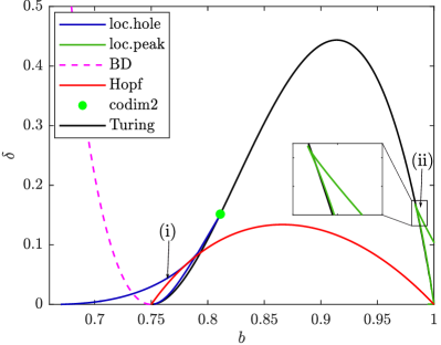
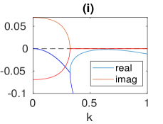
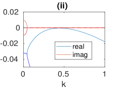
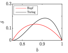
Figure 1: (a) Hopf and Turing instability curves for the homogeneous solution $s_{4}$ of (1) in the $(b,\delta)$ plane when $(a,\alpha,\beta,D)=(1,2,0.5,0.029)$ together with the existence regions for localized patterns. (b) Spectra $\lambda(k)$ at the locations indicated in (a). (c) Bifurcation curves for $D=0.07$ (top) and $D=0.01$ (bottom) showing the dependence of the Turing instability (black curves) on the parameter $D$. The Hopf bifurcation (red curve) is independent of $D$.

In Fig. 1(a) we mark a codimension-two point (green dot), determined from weakly nonlinear theory, where the Turing bifurcation changes from sub– to supercritical. Moreover, we show two curves labeled “localized holes” (blue, on the left) and two labeled “localized peaks” (green, on the right) delimiting the regions of existence of LS. The LS in the former region take the form of finite arrays of large amplitude downward spikes, while the latter consist of upward spikes. Finally, we also show the Belyakov-Devaney (BD) transition curve (dashed purple line), defined by a pair of real spatial eigenvalues of the spatial dynamics problem linearised about the homogeneous equilibrium, each of double multiplicity. This curve is also given by (4) but the corresponding wave number is now imaginary. One major significance of the BD transition is that (standard) snaking of LS typically turns into “foliated snaking” of isolated spikes[32, 25, 1, 14, 3] when crossing the BD line; see Ref.[47] for a general analysis. Here, this region of foliated snaking (to the left of the BD line and below the loc.holes line) is rather small and will not be studied. In Fig. 1(c) we show the instability curves for $D=0.01$ and $D=0.07$. For smaller $D$ the Turing curve expands, while for larger $D$ it shrinks (in (4) $D$ only appears in the combination $\delta D$) while the Hopf curve is unaffected. In both cases we lose the interaction of the Hopf and Turing modes on the left (near (i)), motivating our choice of an intermediate value $D=0.029$ as a starting point for our study.

III Two case studies of localized patterns

We use numerical continuation with pde2path [42] to explore patterns near the two selected instability points from Fig. 1. First, we consider the vicinity of the left point (i), where the primary instability is of Hopf type. However, subcritical Turing instabilities are nearby, leading to localized steady patterns, and we shall see that these inherit, in some sense, the Hopf instability of the homogeneous background. Second, we explore the neighborhood of the right point (ii). Here the primary instability is a supercritical Turing instability, but strongly subcritical sideband instabilities nearby lead to peculiar stable localized patterns, for which the associated snake interpolates between homoclinics to the homogeneous state and homoclinics to small amplitude periodic patterns. For our numerical continuation we choose $\Omega=(-\ell,\ell)$ with $\ell=50$, and plot

$$\|u\|_{2}\mathrel{\mathop{\mathchar 58\relax}}=\sqrt{\frac{1}{2\ell}\int_{-\ell}^{\ell}|u(x)-u^{*}|^{2}\,{\rm d}x},\quad\text{resp.}\quad$$ (6)

$$\|u\|_{2}{\mathrel{\mathop{\mathchar 58\relax}}=}\sqrt{\frac{1}{2T\ell}\int_{0}^{T}\int_{-\ell}^{\ell}|u(x,t){-}u^{*}|^{2}\,{\rm d}x\,{\rm d}t}$$ (7)

for steady, resp. time-periodic states, i.e., we only use the first component of the perturbation from $s_{4}$, and normalize its norm by the domain size (and the period $T$ for time-periodic orbits). The projection $\|u\|_{2}$ as defined is not a norm in the $(u,v)$ space.

III.1 Interaction between LS and background Hopf instability

Figure 2(a), with $\ell=50$, shows that if $b$ is increased at fixed $\delta=0.07$ near location (i), then $s_{4}$ loses stability to a Hopf mode with $k_{c}=0$, i.e., to a spatially uniform oscillation (H1, see the space-time plot at location A in panel (b)). This is followed by a Hopf bifurcation to a spatially nonuniform Hopf mode with wave number $\pi/\ell$ (H2, shown in a space-time plot at location B). Both bifurcations are supercritical, implying that the $k=0$ branch H1 is stable at onset, while the $k=\pi/\ell$ oscillations H2 are unstable at onset, with Floquet index ${\rm ind}=1$ (number of Floquet multipliers $\mu$ with $|\mu|>1$).

The next bifurcation point (BP) from $s_{4}$ yields the first Turing bifurcation (T1, bluebranch, $k=\pi/5\approx 0.628$, profile G). This bifurcation is subcritical, like the next 10 Turing bifurcations, and the “most subcritical” Turing branch is the 6th (T6, dark blue branch, $k=0.534$, profile H).The branch T1 undergoes a secondary bifurcation at small amplitude, i.e., close to the primary bifurcation, to a pair of spatially modulated states which turn into a pair of intertwined snaking branches of localized Turing patterns only one of which (S1, orange branch) is shown in the figure, see profiles at successive fold points FP1 and FP2 in panel (c); owing to NBC these profiles may be reflected in $x=-50$ to generate a localized state on a domain of length 200. As $\ell$ increases this secondary bifurcation moves to smaller amplitude and collides with the primary bifurcation in the limit $\ell\to\infty$.[13]

(a) (b)

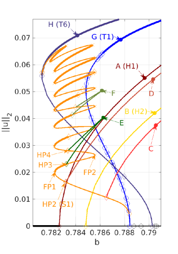
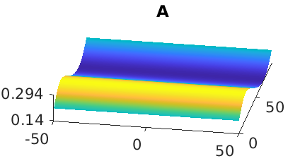
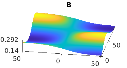
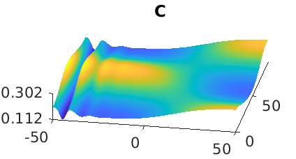
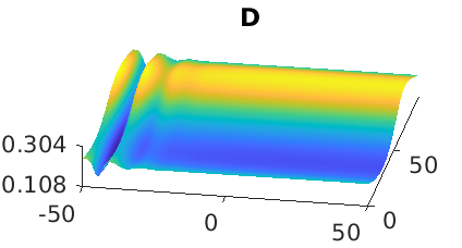
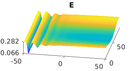
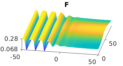
(c)

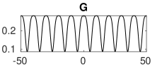
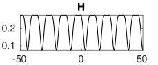
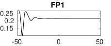
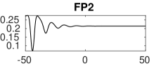
Figure 2: (a) Bifurcation diagram for $\ell=50$ with $(\delta,\alpha,\beta,a,D)=(0.07,2,0.5,1,0.029)$ showing $\|u\|_{2}$ defined in (6) and (7) as a function the parameter $b$ starting from $b=0.78$. (b) Sample time-periodic solutions ($u$ component only) shown in a space-time plot over one temporal period corresponding to the locations labeled in (a). (c) Sample steady solutions ($u$ component only). In (a) Hopf bifurcation points (HPs) are marked by $\diamond$, steady state BPs by $\circ$, and fold points (FPs) by $\times$. Not all HPs, BPs and FPs are shown. For steady states, thick (thin) lines indicate stable (unstable) solution branches. The trivial state $s_{4}$ corresponds to $u=0$. Hopf branches H1 and H2 from this state are shown in brown and yellow, with sample solutions A and B. The primary Turing branch T1 is shown in blue; the 6th Turing branch (T6, dark blue) reaches farthest to the left. A snaking branch of LS (S1, orange) bifurcates from the first BP on T1 and reconnects to T6, sample solutions in (c). Additional HPs on S1 lead to branches with sample solutions (C-F).

Along the orange branch S1 of steady LS the solution adds a wavelength near every other fold until the available domain is filled and the snaking branch terminates on T6. This is a consequence of the fact that the wavelength within the LS is not set by $k_{c}$ but is instead set by nonlinearity and hence the parameter $b$.[13, 9] Note that S1 snakes outside of the region of bistability between $s_{4}$ and T1, despite its origin in T1. Instead the relevant bistability region is the region between $s_{4}$ and T6. On T1 and T6 (and similarly on all other Turing branches, not shown) there are many further BPs, leading to similar secondary bifurcations to localized patterns and snaking branches like the orange branch S1; for instance, the second BP on T1 yields genuine LS on $(-\ell,\ell)$, i.e., double pulse homoclinic orbits on the domain of length 200.

The above behavior is largely consistent with the standard snaking of LS observed in the Swift-Hohenberg equation. The present system is not variational, however, and so time-dependent LS may be expected.[11] Moreover, in the present system snaking occurs in a region of bistability between steady LS and smaller amplitude uniform oscillations on the Hopf branch H1. In this region steady LS cannot be stable over unbounded domains since the background state $s_{4}$ is unstable to oscillations, but stable LS embedded in a time-periodic background may be expected. Evidently, the stability of various states on S1 indicated in Fig. 2(a) is a finite size effect.

Next we consider tertiary Hopf points (HP) on S1. The first two are inherited from the oscillatory instability of $s_{4}$ and generate states that resemble a “superposition” of an LS on S1 and the Hopf modes H2 and H1, see profiles C and D, respectively. In the following we refer to these states as mixed modes (MM). These time-periodic states grow monotonically in amplitude as $b$ increases, and both are unstable. As we continue upward along the S1 branch we find pairs of HPs that are connected by further branches of MMs (green). In each case the lower HP is on a stable part of the LS branch while the upper one is on the next unstable part. Altogether we have 6 pairs of such HPs, all pairwise connected by an MM branch. Similar states were found in Ref.[33], Figs. 13(h) and 14(b), using DNS for suitable values of the predator time scale parameter (our $\delta$) by starting from a localized perturbation of the analog of our $(u^{*},v^{*})$, and in the Gilad-Meron model of dryland plant ecology, also a two-species RD system (Ref.[29], Fig. 9).

We think of these green branches as forming parts of an unzipped “snake”, broken by segments of steady LS (see below for zipping up). Sample solutions at locations E and F are shown in panel (b). In all cases the green segments between the lower HP and the corresponding fold point correspond to stable MMs. We have checked, but do not show, that the intertwined second LS snaking branch (with minima at $x=-50$) undergoes essentially identical behavior with pairs of BPs straddling the right folds and generating partially stable MM segments closely resembling the green branches in Fig. 2(a). These states are also embedded in a uniform background oscillation.

There are two finite domain effects responsible for the existence of stable steady LS connected to the background state $s_{4}$ in a parameter regime in which $s_{4}$ is predicted to be unstable to oscillations: as one proceeds up the S1 branch the LS grow in extent, thereby reducing the domain occupied by $s_{4}$. Figure 1(b), panel (i), shows that as the allowed minimum wave number is pushed to higher values the Hopf bifurcation is suppressed. We expect therefore that the tertiary HPs move to larger values of $b$, as observed. This does not explain, however, the presence of stable narrow LS, such as those created at FP1. In fact FP1 lies below the primary Hopf point for $s_{4}$, and $s_{4}$ is therefore stable at this location. The fact that this state extends stably past the primary Hopf point is a consequence of the fact that once an LS is present the stability of the background state no longer reflects the stability of this state on an unbounded domain (or the equivalent problem with NBC): the smaller oscillation scale at the location of the front between the LS and the background $s_{4}$ enhances dissipation leading to an increase in the critical $b$ for the onset of the Hopf instability, cf. Refs.[36, 5]. Thus the observed behavior is a consequence of both a reduction in the effective domain size, but more importantly of the introduction of a strongly dissipative (non-NBC) boundary at the location of the front separating the LS and the oscillating background. The resulting dissipation suppresses the oscillation amplitude in this region, as evident from the space-time profiles E and F in Fig. 2(b). We remark that once the LS occupies approximately half the domain the role of the LS and the oscillating state changes: it is now more natural to think of a uniform oscillation embedded in a background of a steady periodic pattern.

III.1.1 Zipping up the TH snake

Figures 3 and 4 show how the (green) snake segments reconnect or “zip up” into a full snaking branch of time-periodic states by varying the parameter $D$. In Fig. 3(a), obtained from Hopf-point continuation (HPC) of HP2, HP3 and HP4 on the S1 branch in Fig. 2(a), we show the Hopf point positions $b$ and the corresponding frequencies $\omega$ as $D$ varies. As $D$ increases, the location of HP2 moves up in $b$ while the location of HP3 moves down, resulting in a collision at the fold FP1 of S1 when $D\approx 0.02968$. Similarly, as $D$ decreases, the location of HP3 moves up in $b$ while the location of HP4 moves down, resulting in a collision at FP2 when $D\approx 0.026$. The same happens for HPC of other pairs of Hopf points such as HP5, HP6 and HP7, HP8, etc. Put differently, if we follow HP2 beyond the first collision we obtain the brown curve in Fig. 3(b), a snake of Hopf points. The folds in this curve correspond to successive collisions of Hopf points, HP2 with HP3 at FP1, HP3 with HP4 at FP2 etc. As a result the HP snake is trapped between, say, the FPC of the fold points FP2 (upper boundary) and FP3 (lower boundary) of Fig. 2(a) since the right and left fold points of S1 are almost aligned. Sample solutions corresponding to the locations I, II and III in (b) are shown alongside. Importantly, with increasing $D$, the wedge containing the S1 branch becomes exponentially narrow in $|D-D_{c}|$ with $D_{c}\approx 0.043$, cf. Refs.[15, 19, 18], and overall the structure leans to the right.

Figures 3(c,d) describe steps in the zipping process. In panel (c) we recompute the orange, green and brown curves in Fig. 2(a) for $D\approx 0.02965$. We see that the Hopf points HP2 and HP3 have moved very close to FP1, but the branches bifurcating from HP2 (brown, going to large $b$) and HP3 (green, reconnecting to HP4 on S1) are still distinct. For $D=0.0297$, however, the points HP2 and HP3 on S1 have annihilated one another, resulting in the reconnection of the brown and green branches and the creation of the red branch (panel (c), inset). As a result HP2 and HP3 are absent and the MM branch now originates from HP4 higher up the snaking S1 branch. A further increase in $D$ leads to a collision between HP4 and HP5 at FP3 and the process repeats, resulting in the brown curve in Fig. 3(d) with a footpoint at HP6, just prior to the next collision at FP5.

(a)	(b)

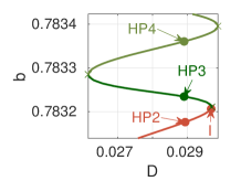
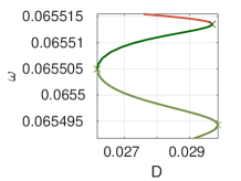
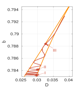
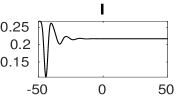
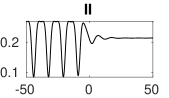
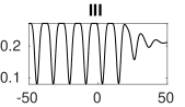
(c)	(d)

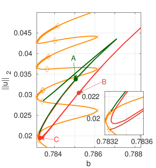
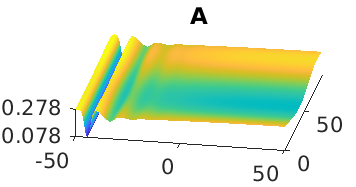
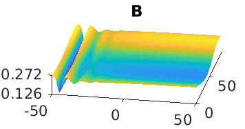
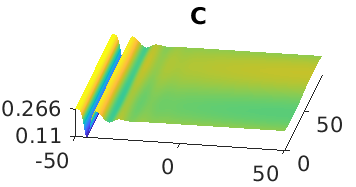
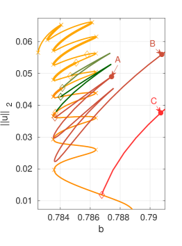
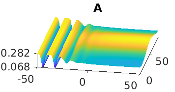
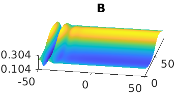
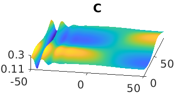
Figure 3: Zipping up the Turing-Hopf segments from Fig. 2 into a Turing-Hopf snake on increasing $D$. (a) HPC of HP2 (brown), HP3 (dark green) and HP4 (light green) from Fig. 2 showing the HP location in the $(D,b)$ plane, together with the corresponding Hopf frequency $\omega$. (b) HPC of HP2 (brown), and FPC of FP2 and FP3 (orange) together with sample solutions I-III used to initialize continuation in $b$ in panels (c) and (d). (c) Bifurcation diagram for $D=0.02965$ corresponding to point I in panel (b); the inset shows the LS branch (orange) near the first fold, shortly before HP2 and HP3 annihilate (at $D=D_{1}\approx 0.02968$) together with the disconnected MM branches (brown and green). The red branch (inset) shows the MM branches at $D=0.0297$, i.e., after reconnection. As a result the large $b$ MM branch now connects to the point HP4 on S1. To generate the red branch we take point A from the green branch at $D=0.02965$, set $D=0.0297$, and continue in $b$. (d) Bifurcation diagram for $D\approx 0.03$ corresponding to point II in panel (b). Stability on S1 is indicated by thick lines; stability on the other branches is not indicated (see text).

In Fig. 4, computed for $D=0.033$, only the (former) HP12 remains, and consequently all the green branches have zipped up and the large $b$ MM branch (brown) now connects to a footpoint at B. Figure 4 also shows the other branches at $D=0.033$, with the same colors as in Fig. 2(a) where applicable. The orange LS snake now reconnects to the 4th Turing branch (dark blue, profile F); a third Hopf branch from $s_{4}$ is now present and is shown in violet (profile E). The details of the switching of the termination point of S1 from T6 to T4 are expected to proceed via T5 and to resemble the process described in Ref.[9] for the Swift-Hohenberg equation but have not been studied in detail in the present case.

The MM segments on the other LS snake intertwined with the S1 snake zip up via a very similar process (not shown). As a result in Fig. 4 there are in fact two intertwined snaking branches of time-periodic MM states, only one of which is shown.

           

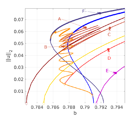
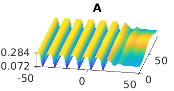
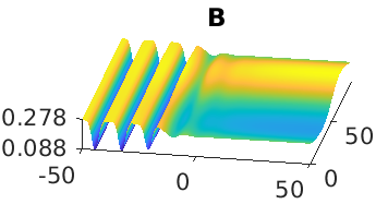
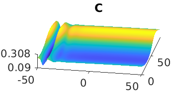
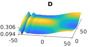
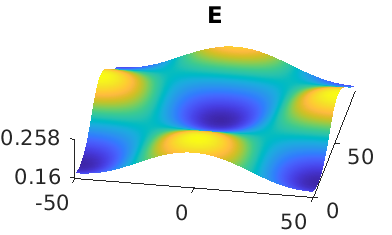
Figure 4: As for Figs. 3(c,d) but for $D=0.033$, corresponding to point III in Fig. 3(b): the whole Turing-Hopf snake has zipped up, generating a snaking branch of time-periodic states terminating near the top of S1 (solutions A-C). Stability is not indicated. The only other HP left on S1 is the one at the bottom leading to the (red, unstable) MM branch with a nonuniform background oscillation (solution D here and solution C in Fig. 3(d)). The figure also shows other branches at $D=0.033$, namely H1 (brown), H2 (yellow), H3 (violet, with sample solution E), as well as T1 (blue) and T4 (4th Turing branch from $s_{4}$, dark blue with sample solution F), the termination of S1 for this value of $D$.

We refer to the brown branch from Fig. 4 as a Turing-Hopf (TH) snake. The space-time profiles show that the TH snake recapitulates the behavior of the S1 snake, albeit in a larger and shifted parameter interval. In particular, as one proceeds up the TH snake, the (almost) stationary core of the solution adds a new wavelength during every back and forth oscillation of the branch, restricting the oscillating background to an ever smaller part of the spatial domain. The progressive nature of the zipping up process is a consequence of this fact which results in HP collisions that are staggered in $D$ (Fig. 3(b)). This follows from the fact that as the central LS structure of the oscillations expands it becomes harder to excite oscillations in the rest of the available domain. In larger domains, therefore, the zipping process may be faster. The process itself has one major consequence: it progressively erases the stability of the steady LS states and “replaces” these states by coexisting stable segments of time-periodic states that extend over a wider parameter interval. These states resemble the steady LS in their center but are embedded in an oscillating background. The light red branch that bifurcates from HP1 on S1 (solutions C in Fig. 3(d) and D in Fig. 4) is qualitatively unaffected by the small changes in $D$ required to zip the TH snake.

(a)

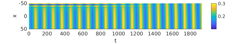
(b)

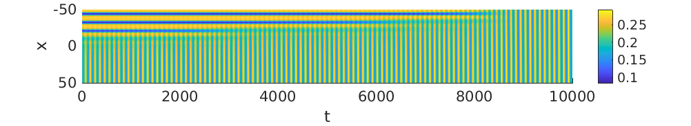
(c)

(d)

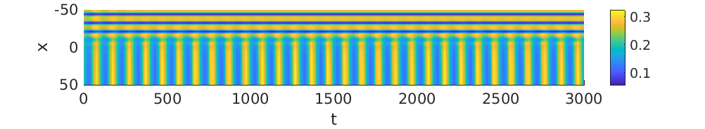
Figure 5: DNS from marked points (+small perturbation) in Fig. 4(a). (a) Starting from C with fast convergence to H1. (b) Starting from B with slow convergence to H1. (c) Starting from B but setting $b=b+0.015$ (right of the TH snake), yielding (stick–slip) convergence to T4. (d) Starting from B but setting $b=b+0.007$, yielding convergence to a stable MM in the TH snake.

Remark III.1

a) The collision of HP2 with HP3 on S1 (Figs. 3(a,c)) occurs when their two frequencies and respective eigenfunctions become identical. The resulting double Hopf bifurcation with 1:1 resonance corresponds to a nilpotent bifurcation, described by a normal form derived and studied in Ref.[46]. However, resonant bifurcations of this type are codimension–3 bifurcations, and are therefore not expected when only two parameters such as $b$ and $D$ are varied. This is because two parameters are required to generate a double Hopf bifurcation in the first place, and a third parameter is required to tune their frequencies into resonance. No reconnection takes place when the frequencies are incommensurate – the bifurcations pass through one another. The required resonance forces the resonant double Hopf bifurcation to occur at the fold FP1, and similarly for all the subsequent collisions and associated reconnections. Nominally, a 1:1 double Hopf bifurcation at FP1 is a codimension–4 event but the fact that this forces $d\omega_{1}/dD=d\omega_{2}/dD=\infty$ (Fig. 3(a)), in addition to $\omega_{1}=\omega_{2}$, makes the problem codimension–2, as documented in Fig. 3(b). Simply put, reconnection cannot occur generically unless it takes place via the fold points FP on S1.

b) In Fig. 5 we briefly look at DNS from selected points in and near the TH snake from Fig. 3(c) obtained from initial conditions corresponding to these points but increasing the parameter $b$ by a small amount. Panel (a) shows a space-time representation of a solution starting from point C; the solution evolves into a stable H1 oscillation. Panel (b) starts from point B and also evolves into H1 albeit much more slowly. Panel (c) also starts from point B but with $b$ increased by $\Delta b=0.015$; this time the state evolves into a stable spatially periodic state on the T4 branch. Finally, panel (d) starts from point B but with $\Delta b=0.007$; the solution converges to a stable MM state on a green MM branch right above that shown in the figure. Each of these four panels shows an advancing or retreating front between two states (steady or oscillating) that exhibits stick-slip motion, much as in the Swift-Hohenberg equation.[12] Evidently in this region, both before and after the zipping up process, the system exhibits extreme multistability that increases with the domain size $\ell$.

c) Hopf instabilities of LS can also appear in a form other than as “background oscillations” in Fig. 2, namely in the form of “breathing peaks”, where the background remains at rest but the localized state oscillates. See, e.g., Refs. [2, 1]. However, such breathing peaks have not been found in (1).

d) For background Hopf wave number $k_{H}\neq 0$ the background oscillations can organize either into traveling or standing waves depending on parameters.[21] However, since the onset of the $k_{H}\neq 0$ oscillations is preceded by the $k_{H}=0$ onset, both of these states are expected to be unstable. In a related problem arising in binary fluid convection driven by the Marangoni effect[4] the background is unstable with respect to $k_{H}\neq 0$ oscillations and fills with standing waves, with the constituent left-traveling waves dominant to the right of the LS and right-traveling waves dominant to the left – a consequence of the effective boundary conditions at the location of the front(s) separating the oscillations from the nearly steady LS.

e) Throughout this paper we have computed solutions on the half-domain imposing reflection symmetry in $x=-\ell$ to generate even solutions on a domain of length $4\ell$. Because of this procedure we can only compute snaking branches of even states. However, just as in the case of steady LS there is a family of of time-periodic states with odd symmetry in $x=-\ell$ and hence a pair of intertwined branches of even and odd time-periodic states on a domain of length $4\ell$. $\rfloor$

III.1.2 Continuation of Hopf and fold points in $\delta$

Figure 6(a) shows continuation results of bifurcation points from Fig. 2 as functions of the parameter $\delta$ when $(\alpha,\beta,a,D)=(2,0.5,1,0.029)$. In this case the HPC never reaches the left folds and therefore no zipping up takes place. Panel (b) shows the continuation in $b$ from point A, $\delta\approx 0.056$. There are two main differences compared to Fig. 2(a): there are now three primary Hopf branches that bifurcate from $s_{4}$ at “low” $b$, i.e., in the $b$ range of the S1 snake, with the branch H3 (violet) of spatially dependent background oscillations with wave number $k=2\pi/100$ (solution D in panel (c) or solution E in Fig. 4) “moving in” to lower $b$. As a consequence, at the bottom of the S1 snake there is a new HP giving rise to the pink branch of mixed mode oscillations in the form of a superposition of the LS from S1 and the $k=2\pi/100$ background oscillation. At the same time two new HPs with background wave number $k=\pi/100$ appear on the S1 snake, inherited from H2 (yellow branch) and straddling FP2, yielding a second connecting segment (purple) of oscillations, this time with the background wave number $k=\pi/100$. These MM states, like those in green, extend far outside the S1 snaking range. On larger domains, we find additional pairs of HPs near the right folds of the S1 snake, but here only one is present since the growth of the LS along S1 suppresses the $k=\pi/100$ oscillations in the background. Moreover, on larger domains the $k\neq 0$ segments again zip up when $D$ is varied (not shown). We anticipate that for other parameter values (and/or larger domains) the solution structure of mixed modes will incorporate states with yet more complex background oscillations. However, these new mixed mode oscillations are all expected to be unstable owing to the instability of the $k\neq 0$ background oscillations with respect to $k=0$ oscillations.

(a)	(b)	(c)

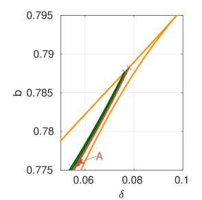
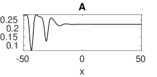
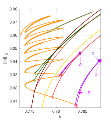
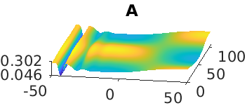
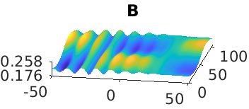
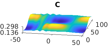
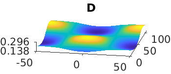
Figure 6: As for Fig. 2 but showing the dependence on the parameter $\delta$ instead of $D$. (a) The $(\delta,b)$ plane, with FPC of FP1 and FP2 (orange), and HPC of HP2 (brown) and HP7 (green), with a sample solution profile at $\delta\approx 0.056$. (b) Bifurcation diagram at $\delta=0.056$; the branches already present in Fig. 2 (same colors here) behave as before but extend farther to the right, and there are two new (unstable) Hopf branches: one secondary mixed mode branch (pink, profiles B and C) with background wavenumber $2\pi/100$, and the corresponding connection on S1 (purple, profile A), analogous to the green branches with $k=0$ background oscillation.

III.2 Supercritical Turing instability and localized patterns

Spatially localized patterns are usually associated with subcritical instabilities, such as the subcritical Turing instability; see, e.g., Refs.[10, 25]. However, as discussed below, LS may be found even when the Turing bifurcation is supercritical. In Fig. 7 we illustrate the behavior of (1) on the right of the Turing region in Fig. 1, more specifically near location (ii). This is far from the Hopf instability of $s_{4}$, and indeed Hopf instabilities no longer play a role in Fig. 7. Moreover, this region is located to the right of the green point in Fig. 1, in a region where the primary Turing bifurcation is supercritical. In general snaking is not expected in the supercritical regime, owing to the absence of bistability. An exception is provided by systems with a conservation law such as the conserved Swift-Hohenberg equation[35] where a secondary, strongly subcritical instability may destabilize a supercritical Turing state at small amplitude, generating LS exhibiting (slanted) snaking in a parameter regime with no bistability. Similar small amplitude secondary instabilities have also been found in other conserved systems such a rotating convection between free-slip boundaries.[7]

(a) (b)

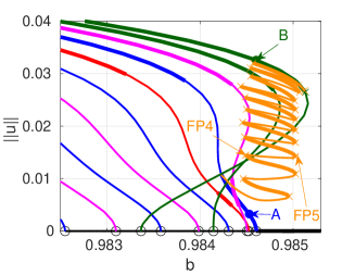
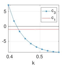
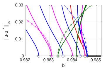
(c)

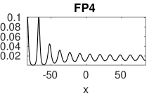
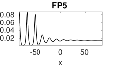
Figure 7: Bifurcation behavior in region (ii): $(\delta,\alpha,\beta,a,D)=(0.16,2,0.5,1,0.029)$ with $\ell=12\pi/k_{c}$ and $b$ as the primary bifurcation parameter. The onset wave number is $k_{c}=0.4505$ (T1, blue branch). (a) Bifurcation diagram showing branches T1–T9 (see Table 1 for colors) together with the S1 snake (orange). (b) Dependence of the Landau coefficients on the wave number $k$ together with a comparison between the solution branches determined from numerical continuation (panel (a)) and the Landau approximation to selected branches. (c) Sample solution profiles ($u$ component only) at locations labeled in (a).

Even without a conservation law, Eq. (1) supports LS in the supercritical region (ii) but for a different reason. Figure 7 shows that the primary Turing branch (T1, blue) loses stability shortly after bifurcation to a (nonslanted) branch (S1, orange) of snaking localized patterns. Near the right folds of this structure the LS are embedded in the stable $s_{4}$ state (solution FP5). However, the snake extends across the primary bifurcation to T1 and solutions in this region are instead embedded in a small amplitude periodic Turing pattern (solution A) as shown by solution FP4. The transition between these two situation is smooth, with no change in stability. Similar states were found inrotating plane Couette flow[34] and in natural binary fluid convection[37], and were studied in Ref.[23] in a model problem, the 3-5-7 Swift-Hohenberg equation; here we find that they arise in a natural way in the RD system (1).

To understand the behavior shown in Fig. 7 we computed the Landau coefficients $c_{1}$ and $c_{3}$ that describe the small amplitude behavior of the Turing branches. The Landau approximation for the branch T_j with wave number $k_{j}$ bifurcating at $b=b_{T_{j}}=\mathrel{\mathop{\mathchar 58\relax}}b_{j}$ is given by

$$(u,v)(t,x) -(u,v)^{*}(b_{j})=\varepsilon A(T){\rm e}^{{\rm i}k_{j}x}\phi(k_{j})$$

$$+\varepsilon^{2}\biggl{[}\frac{1}{2}A_{0}(T)+A_{2}(T){\rm e}^{2{\rm i}k_{j}x}\biggr{]}+\rm c.c.+\rm h.o.t.,$$ (8a)

where $\phi_{j}\equiv\phi(k_{j})\in{\mathbb{R}}^{2}$ is a kernel vector of $J|_{(u,v)^{*}(b_{j})}-k_{j}^{2}{\cal D}$ (in the following normalized to $\phi_{j,1}=1$), $0<\varepsilon\ll 1$ is a formal perturbation parameter, and $\rm h.o.t.$ denotes higher order terms. In general the complex amplitude function $A$ depends on the slow time scale $T=\varepsilon^{2}t$ while $A_{0}(T)\in{\mathbb{R}}^{2}$ and $A_{2}(T)\in{\mathbb{C}}^{2}$ are the modes excited at second order. Substituting (8) into Eq. (1), all terms at ${\cal O}(\varepsilon)$ vanish, while at ${\cal O}(\varepsilon^{2})$ we obtain equations for $A_{0}$ and $A_{2}$. At ${\cal O}(\varepsilon^{3})$ a solvability condition required to avoid secular growth of $A$ gives the equation

$$A_{T}=c_{1}(b-b_{j})A+c_{3}|A|^{2}A,$$ (9)

where we replaced $\varepsilon$ by $\sqrt{|b-b_{j}|}$, and $c_{1}\equiv{\partial}_{b}\lambda_{1}(b_{j},k_{j})$ and $c_{3}$ are the Landau coefficients. The (analytical) computation of $c_{1}$ and $c_{3}$ is in principle straightforward but can be rather cumbersome, and we restrict the discussion that follows to their numerical evaluation using the ampsys tool of pde2path [44], and list their values in Table 1. To approximate the Turing branches we may look for steady (and without loss of generality real) solutions of (9), given by $A=0$ and

$$A=\sqrt{-c_{1}(b-b_{j})/c_{3}},$$ (10)

with $b>b_{j}$ if $c_{1}/c_{3}<0$ (the subcritical regime in our case) and $b<b_{j}$ if $c_{1}/c_{3}>0$ (the supercritical regime). For illustration, in Fig. 7(c) we compare $|u_{1}-u^{*}(b)|$ obtained from numerical continuation of the Turing branches (panel (a)) with their first order Landau approximations, i.e., with $A$ from (10); this means a comparison with $u^{*}(b_{j})+2A\cos(k_{j}x)-u^{*}(b)$, and since $\sup_{x}\cos(kx)=1$, the dotted branches are given by $2A-(b-b_{j})$.

The key reason for the unexpected snaking revealed in panel (a) is the strong sensitivity of $c_{3}$ to $k$ and the sign change of $k\mapsto c_{3}(k)$ near $k\approx 0.42$ (see the green branches T5 and T8 in panel (b)), together with the nonmonotonic order of the primary BPs, with branches of smaller wave number (solution B in (a)) interspersed with branches of higher wave number (solution A in (a)). This effectively yields bistability in the present system despite the fact that the primary branch T1 is supercritical. Figure 7(a) shows that the low wave number branches T5 and T8 are strongly subcritical and hence extend substantially past the primary T1 Turing bifurcation. Of these the T8 branch (green) extends to the largest values of the parameter $b$ and yields the widest interval of bistability with stable $s_{4}$ and this is indeed the branch on which the orange snaking branch terminates.

Name	T1	T2	T3	T4	T5	T6	T7	T8	T9
color	blue	red	mag	blue	green	mag	blue	green	mag
$b|_{BP}$	0.9846	0.98452	0.98451	0.98431	0.98414	0.98399	0.98358	0.98337	0.9831
$n$	12	12.5	11.5	13	11	13.5	14	10.5	14.5
$k$	$k_{c}$	0.46927	0.43172	0.48804	0.41295	0.50681	0.52558	0.39418	0.54435
$c_{1}$	-1.0078	-1.0040	-1.0124	-1.0006	-1.0181	-0.9973	-0.9946	-1.02534	-0.9917
$c_{3}$	-4.1310	-5.8033	-1.7144	-6.9483	1.8053	-7.7145	-8.2141	7.2065	-8.5241

Table 1: Data for the first 9 Turing branches from Fig. 7 for $(\delta,\alpha,\beta,a,D){=}(0.16,2,0.5,1,0.029)$, $k_{c}{=}0.4505$, showing the branching points $b|_{BP}$ for solutions with wave numbers $k=k_{c}n/12$, where $n$ is the number of wavelengths on a domain of length $\ell=24\pi/k_{c}$ together with the corresponding Landau coefficients $c_{1}$ and $c_{3}$.

IV Zipping up a TH snake in the Gilad–Meron model

In this section we demonstrate that the zipping process in Figs. 2-4 also occurs in another RD system and can thus be considered generic. We consider the so-called simplified Gilad-Meron (sGM) model for vegetation patterns in drylands with sandy soil where surface water flow is not a major factor. The model considers the biomass of the above-ground vegetation, denoted by $b(x,t)$, and the soil-water content, represented by $w(x,t)$, and in dimensionless form reads[49]

$$\partial_{t}b =bw\left(1+\eta b\right)^{2}\left(1-b\right)-b+D\partial_{x}^{2}b,$$ (11a)

$$\partial_{t}w =p-\displaystyle{\frac{nw}{1+\rho b}}-\alpha bw\left(1+\eta b\right)^{2}+\partial_{x}^{2}w,\quad$$ (11b)

where $\eta$ is the root-to-shoot ratio of the plants, $p$ is the precipitation rate, $\alpha$ is the water uptake efficiency, $n$ is the evaporation rate, and $\rho$ describes the reduction of evaporation resulting from the presence of biomass. A linear and nonlinear stability analysis for (11) is available in Ref.[29], together with bifurcation diagrams showing various LS branches and the secondary Hopf bifurcations from LS leading to short segments of mixed TH states (Ref.[29], Fig. 9) as in Fig. 2 for the system (1).

(a)	(b)	(d)
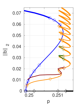
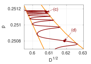
	(c)

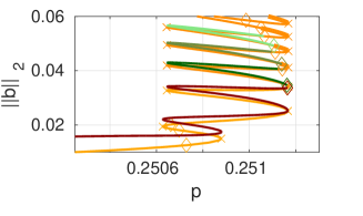
Figure 8: Zipping up the TH snake for the sGM model (11) with $\ell{=}60$ and $(n,\eta,\rho,\alpha){=}(0.3579,3.5,0.6,1,0.5)$. (a) Bifurcation diagram for $D=0.36$ as a function of the parameter $p$ showing the primary Turing branch (blue), a steady LS snake (orange), and two short TH segments (green). (b) HPC of HP4 (brown), and FPC of FP5 and FP6 (orange) in the $(D,p)$ plane for comparison with Fig. 3(b). (c) Bifurcation diagram at location (c) in (b), $D=0.37$; (the former) HP4 and HP5 have anniliated, and the brown TH branch now starts at HP6. (d) Bifurcation diagram at location (d) in (b), $D=0.383$.

Figure 8 shows that we can zip up these segments into a TH snake, exactly as in Figs. 2-4 for the system (1). Panel (a) displays the starting situation on a domain slightly smaller ($\ell=60$) than that in Ref.[29], Fig. 9. For the “norm” $\|b\|_{2}$ we again use (6),(7), where the steady state $b^{*}$ of uniform vegetation is computed numerically at the given parameter values. The first three bifurcations from the black branch (at $\|b\|_{2}=0$) are of Hopf type, and at $p=p_{T}\approx 0.2499$ we find the first Turing branch (T1, blue), with a secondary bifurcation to an LS snaking branch at small amplitude (S1, orange). The first two HPs on this branch are associated to $k\neq 0$ Hopf bifurcations of the background while the third belongs to a $k=0$ Hopf bifurcation of the background and the associated brown branch extends down to $p<0.2499$. The remaining HPs on the LS snake S1 are pairwise connected by short segments, two of which are shown in green. Panel (b), similar to Fig. 3(b), illustrates the HPC (brown) of HP4 in the parameter $D$ together with the FPC of FP5 and FP6. The HP moves through folds given by the FPC, i.e., at these folds two HPs collide and annihilate, and the brown branch shows the HP crossing from one HP in (a) to the next. In panel (c), HP4 and HP5 have annihilated, and the brown branch now starts at the (former) HP6, positioned farther up the orange snake. In panel (d), all the former short green segments (except for the topmost) have reconnected into a long snaking TH branch. In contrast to Fig. 4, however, this time both the green MM segments, and the zipped up TH branch (brown) span the same $p$ range as the LS snake (orange).

V Discussion

We have revisited the Hopf-Turing interaction that arises in a number of two-species reaction-diffusion systems.[17, 27, 39, 41] In particular, in Ref.[17] the authors considered the Brusselator model with supercritical Hopf and Turing branches in a regime with bistability between the two, finding a large multiplicity of stable Turing states embedded in an oscillating background obtained via DNS. Since no continuation was performed the observed states were not linked to homoclinic snaking, a notion that was developed only subsequently.[52] The present work differs in that we consider a case in which the Turing bifurcation is subcritical. This case, already considered in Ref.[41], is more interesting since it admits a variety of steady LS embedded in a homogeneous background. When the Turing bifurcation is preceded by a (supercritical) Hopf bifurcation, the homogeneous background is no longer time-independent but begins to oscillate. States of this type were computed in Ref.[41] but their bifurcation behavior was not studied in any detail. The present work seeks to develop further understanding of these time-periodic LS, focusing on the model (1). This model, like the Brusselator model studied in Ref.[17], also leads to bistability between the Hopf and Turing states, but this time there is more: the Turing bifurcation is associated with a snaking branch of steady LS embedded in a trivial state, as also found in Ref.[41]. We have seen that in the bistability region these LS undergo a series of Hopf bifurcations inherited from the primary Hopf bifurcation that lead to LS embedded in an oscillating background. We found that for some parameter values these oscillatory states extend between pairs of Hopf bifurcations on the snaking LS branch, one on either side of every right fold. Remarkably, we found that by varying a second parameter we could progressively move a secondary Hopf bifurcation to a small amplitude mixed mode up the LS branch, leading to repeated reconnection between the mixed mode and the disconnected oscillatory states on the LS branch. We described the net effect of these reconnections as zipping up of these disconnected branches into a snaking branch of oscillatory states and demonstrated that similar zipping up occurs in other RD systems such as the simplified Gilad-Meron model. We believe our study presents perhaps the best example of this behavior in a two-species RD system, and the most compelling example of snaking of spatially localized time-periodic states. Similar zipping transitions arise in forced snaking[32] and are studied in detail in Ref.[30], albeit for steady LS only. See also Refs.[48, 37].

Once a TH snake is established as in Fig. 4 for (1) by varying $b$, or in Fig. 8 for (11) by varying $p$, we can choose a point from such branches and find snaking behavior on continuing that point in some other parameter. Thus the primary parameters $b$ in (1) and $p$ in (11) are essentially just convenient standard choices. However, in both our models (1) and (11), we need to use the diffusion constant $D$ for the zipping up of the TH snake, i.e., to the best of our knowledge a similar zipping up is not possible using two–parameter continuation that excludes $D$; see Fig. 6 for an example using $(b,\delta)$ in (1). Technically, the explanation for the zipping up is given in Remark III.1a). This remark applies to (11) as well, but why this occurs in both models under Hopf–point continuation in $D$ but not other parameters warrants further investigation.

Surprisingly, we also found homoclinic snaking in the regime where the Turing bifurcation of the trivial state comes in first and is supercritical, a consequence of a strongly subcritical secondary bifurcation to spatially modulated states that extend well into the regime of stable trivial states. The resulting LS are then embedded in the trivial state but when this state becomes Turing-unstable they connect to a small amplitude Turing state in the background. These LS were found to snake (and hence acquire stability) owing to bistability with strongly subcritical sideband Turing states. We traced this behavior to the nonmonotonic order of the primary bifurcation points with respect to the wave number $k$ together with the fact that the key Landau coefficient $c_{3}$ depends sensitively on $k$ and changes sign near $k_{c}$. It must be emphasized, however, that whenever the LS are embedded in a periodic background the imposed domain size plays a significant role. This is in addition to its role in determining the order of the primary BPs to the various sidebranches associated with the Turing instability.

Altogether, our results add to the variety, multistability, and competition between patterned or spatially localized steady states and time–periodic states of two–component RD systems. For instance, Fig. 5 illustrates that in the vicinity of a TH snake very different long–time behavior may be found, depending both on the details of the initial condition and the parameter value. Moreover, the zipping up of the even TH snake (and a similar zipping up of the odd TH snake – not shown) generates a pair of intertwined snaking branches of time-periodic states and hence a large multiplicity of coexisting time-periodic states of either parity, in complete analogy with the snaking of steady LS, thereby explaining why LS embedded in an oscillatory background may occur in systems with arbitrarily large spatial extent.

There is a natural extension of the present work, and that is to three-species RD systems. These systems may exhibit, in appropriate parameter regimes, a wave instability, i.e., a Hopf bifurcation with a finite wave number. This instability may develop into standing or traveling waves, depending on parameters.[21] We anticipate therefore that in such systems we may be able to compute LS embedded in a background of standing or traveling waves, depending on parameters, as already found for Marangoni driven convection.[4] In two-species systems such a bifurcation is never the first instability for which $k_{H}=0$ but we have seen that $k_{H}\neq 0$ states can set in in subsequent primary Hopf bifurcations, and that this bifurcation can likewise be inherited by the secondary LS, resulting in spatially localized time-periodic structures. It is of interest to determine whether these states also snake. We mention that numerically stable steady LS are found even when the background trivial state is unstable to traveling waves, provided it is only convectively unstable.[5, 50] Thus the three-species case is expected to be considerably richer than the system (1) studied here.

Acknowledgement. The work of EK was supported in part by the National Science Foundation under Grant No. DMS-1908891.

References

- [1] F. Al Saadi, A. R. Champneys, and N. Verschueren. Localized patterns and semi-strong interaction, a unifying framework for reaction–diffusion systems. IMA J. Appl. Math., 86:1031–1065, 2021.
- [2] F. Al Saadi, A. Worthy, H. Alrihieli, and M. Nelson. Localised spatial structures in the Thomas model. Mathematics and Computers in Simulation, 194:141–158, 2022.
- [3] F. Al Saadi, A. Worthy, J. R. Pillai, and A. Msmali. Localised structures in a virus-host model. Journal of Mathematical Analysis and Applications, 499:125014, 2021.
- [4] P. Assemat, A. Bergeon, and E. Knobloch. Spatially localized states in Marangoni convection in binary mixtures. Fluid Dyn. Res., 40:852–876, 2008.
- [5] O. Batiste, E. Knobloch, A. Alonso, and I. Mercader. Spatially localized binary fluid convection. J. Fluid Mech., 560:149–158, 2006.
- [6] A. D. Bazykin. Nonlinear Dynamics of Interacting Populations. World Scientific, 1998.
- [7] C. Beaume, A. Bergeon, H.-C. Kao, and E. Knobloch. Convectons in a rotating fluid layer. J. Fluid Mech., 717:417–448, 2013.
- [8] M. Beck, J. Knobloch, D. J. B. Lloyd, B. Sandstede, and T. Wagenknecht. Snakes, ladders, and isolas of localized patterns. SIAM J. Math. Anal., 41:936–972, 2009.
- [9] A. Bergeon, J. Burke, E. Knobloch, and I. Mercader. Eckhaus instability and homoclinic snaking. Phys. Rev. E, 78:046201, 2008.
- [10] V. Breña-Medina and A. R. Champneys. Subcritical Turing bifurcation and the morphogenesis of localized patterns. Phys. Rev. E, 90:032923, 2014.
- [11] J. Burke and J. H. P. Dawes. Localized states in an extended Swift–Hohenberg equation. SIAM J. Appl. Dyn. Syst., 11:261–284, 2012.
- [12] J. Burke and E. Knobloch. Localized states in the generalized Swift-Hohenberg equation. Phys. Rev. E, 73:056211, 2006.
- [13] J. Burke and E. Knobloch. Homoclinic snaking: Structure and stability. Chaos, 17:037102, 2007.
- [14] A. R. Champneys. Homoclinic orbits in reversible systems and their applications in mechanics, fluids and optics. Physica D, 112:158–186, 1998.
- [15] S. J. Chapman and G. Kozyreff. Exponential asymptotics of localised patterns and snaking bifurcation diagrams. Physica D, 238:319–354, 2009.
- [16] J. H. P. Dawes. Localized pattern formation with a large-scale mode: slanted snaking. SIAM J. Appl. Dyn. Syst., 7:186–206, 2008.
- [17] A. De Wit, D. Lima, G. Dewel, and P. Borckmans. Spatiotemporal dynamics near a codimension-two point. Phys. Rev. E, 54:261–271, 1996.
- [18] H. de Witt. Beyond all order asymptotics for homoclinic snaking in a Schnakenberg system. Nonlinearity, 32:2667–2693, 2019.
- [19] A. D. Dean, P. C. Matthews, S. M. Cox, and J. R. King. Exponential asymptotics of homoclinic snaking. Nonlinearity, 24:3323–3351, 2011.
- [20] W. J. Firth, L. Columbo, and A. J. Scroggie. Proposed resolution of theory-experiment discrepancy in homoclinic snaking. Phys. Rev. Lett., 99:104503, 2007.
- [21] E. Knobloch. Oscillatory convection in binary mixtures. Phys. Rev. A, 34:1538–1549, 1986.
- [22] E. Knobloch. Spatial localization in dissipative systems. Annu. Rev. Cond. Matter Phys., 6:325–359, 2015.
- [23] E. Knobloch, H. Uecker, and D. Wetzel. Defect–like structures and localized patterns in the cubic-quintic-septic Swift–Hohenberg equation. Phys. Rev. E, 100:012204, 2019.
- [24] E. Knobloch, H. Uecker, and A. Yochelis. Origin of jumping oscillons in an excitable reaction-diffusion system. Phys. Rev. E, 104:L062201, 2021.
- [25] E. Knobloch and A. Yochelis. Stationary peaks in a multivariable reaction-diffusion system: Foliated snaking due to subcritical Turing instability. IMA J. Appl. Math., 86:1066–1093, 2021.
- [26] D. Lo Jacono, A. Bergeon, and E. Knobloch. Localized traveling pulses in natural doubly diffusive convection. Phys. Rev. Fluids, 2:093501, 2017.
- [27] M. Meixner, A. De Wit, S. Bose, and E. Schöll. Generic spatiotemporal dynamics near codimension-two Turing-Hopf bifurcations. Phys. Rev. E, 55:6690–6697, 1997.
- [28] These curves were computed by fold-continuation of selected folds of LS; as explained below, it is in general not clear which LS (i.e., of which width and wave number) extends farthest in the plane, and hence these lines provide an approximate characterization only.
- [29] P. Parra-Rivas and F. Al Saadi. Transitions between dissipative localized structures in the simplified Gilad-Meron model for dryland plant ecology. Chaos, 33:033129, 2023.
- [30] P. Parra-Rivas, A. R. Champneys, F. Al Saadi, D. Gomila, and E. Knobloch. Organization of spatially localized structures near a codimension-three cusp-Turing bifurcation. SIAM J. Appl. Dyn. Syst., 22:2693–2731, 2023.
- [31] Y. Pomeau. Front motion, metastability and subcritical bifurcations in hydrodynamics. Physica D, 23:3–11, 1986.
- [32] B. Ponedel and E. Knobloch. Forced snaking: Localized structures in the real Ginzburg–Landau equation with spatially periodic parametric forcing. Eur. Phys. J. Special Topics, 225:2549–2561, 2016.
- [33] P. Roy Chowdhury, S. Petrovskii, V. Volpert, and M. Banerjee. Attractors and long transients in a spatio-temporal slow-fast Bazykin’s model. Commun. Nonlinear Sci. Numer. Simul., 118:107014, 2023.
- [34] M. Salewski, J. F. Gibson, and T. M. Schneider. The origin of localized snakes-and-ladders solutions of plane Couette flow. Phys. Rev. E, 100:031102(R), 2019.
- [35] U. Thiele, A. J. Archer, M. J. Robbins, H. Gomez, and E. Knobloch. Localized states in the conserved Swift–Hohenberg equation with cubic nonlinearity. Phys. Rev. E, 87:042915, 2013.
- [36] S. Tobias, M. R. E. Proctor, and E. Knobloch. Convective and absolute instabilities of fluid flows in finite geometry. Physica D, 113:43–72, 1998.
- [37] J. Tumelty, C. Beaume, and A. M. Rucklidge. Toward convectons in the supercritical regime: homoclinic snaking in natural doubly diffusive convection. SIAM J. Appl. Dyn. Syst., 22:1710–1742, 2023.
- [38] J. C. Tzou, A. Bayliss, B. J. Matkowsky, and V. A. Volpert. Interaction of Turing and Hopf modes in the superdiffusive Brusselator model near a codimension two bifurcation point. Math. Model. Nat. Phenom., 6:87–118, 2011.
- [39] J. C. Tzou, Y. P. Ma, A. Bayliss, B. J. Matkowsky, and V. A. Volpert. Homoclinic snaking near a codimension-two Turing–Hopf bifurcation bifurcation point in the Brusselator model. Phys. Rev. E, 87:022908, 2013.
- [40] J. C. Tzou, B. J. Matkowsky, and V. A. Volpert. Interaction of Turing and Hopf modes in the superdiffusive Brusselator model. Appl. Math. Lett., 22:1432–1437, 2009.
- [41] H. Uecker. Continuation and bifurcation for nonlinear PDEs – algorithms, applications, and experiments. Jahresbericht DMV, 124:43–80, 2021.
- [42] H. Uecker. Numerical Continuation and Bifurcation in Nonlinear PDEs. SIAM, Philadelphia, PA, 2021.
- [43] H. Uecker and D. Wetzel. Numerical results for snaking of patterns over patterns in some 2D Selkov–Schnakenberg reaction-diffusion systems. SIAM J. Appl. Dyn. Syst., 13:94–128, 2014.
- [44] H. Uecker and D. Wetzel. The ampsys tool of pde2path, arxiv 1906.10622, 2019.
- [45] H. Uecker and D. Wetzel. Snaking branches of planar BCC fronts in the 3D Brusselator. Physica D, 406:132383, 2020.
- [46] S. A. van Gils, M. Krupa, and W. F. Langford. Hopf bifurcation with non-semisimple 1:1 resonance. Nonlinearity, 3:825–850, 1990.
- [47] N. Verschueren and A. R. Champneys. Dissecting the snake: Transition from localized patterns to spike solutions. Physica D, 419:132858, 2021.
- [48] N. Verschueren, E. Knobloch, and H. Uecker. Localized and extended patterns in the cubic-quintic Swift–Hohenberg equation on a disk. Phys. Rev. E, 104:014208, 2021.
- [49] J. von Hardenberg, A. Provencale, P. Parra-Rivas, and E. Meron. Ecosystem engineers: from pattern formation to habitat creation. Phys. Rev. Lett., 93:098105, 2004.
- [50] T. Watanabe, M. Iima, and Y. Nishiura. Spontaneous formation of travelling localized structures and their asymptotic behaviour in binary fluid convection. J. Fluid Mech., 712:219–243, 2012.
- [51] D. Wetzel. Tristability between stripes, up-hexagons, and down-hexagons and snaking bifurcation branches of spatial connections between up- and down-hexagons. Phys. Rev. E, 97:062221, 2018.
- [52] P. D. Woods and A. R. Champneys. Heteroclinic tangles and homoclinic snaking in the unfolding of a degenerate reversible Hamiltonian-Hopf bifurcation. Physica D, 129:147–170, 1999.
- [53] J. Zhou. Positive solutions of a diffusive Leslie–Gower predator–prey model with Bazykin functional response. Zeitschrift für angewandte Mathematik und Physik, 65:1–18, 2014.
- [54] J. Zhou. Bifurcation analysis of a diffusive predator-prey model with Bazykin functional response. Int. J. Bif. Chaos Appl. Sci. Engrg., 29:1950136, 2019.