Optimal control of spin qudits subject to decoherence using amplitude-and-frequency-constrained pulses

Abstract

Quantum optimal control theory (QOCT) can be used to design the shape of electromagnetic pulses that implement operations on quantum devices. By using non-trivially shaped waveforms, gates can be made significantly faster than those built by concatenating monochromatic pulses. Recently, we applied this technique to the control of molecular spin qudits modelled with Schrödinger’s equation and showed it can speed up operations, helping mitigate the effects of decoherence [Phys. Rev. Appl. 17, 064028 (2022)]. However, short gate times result in large optimal pulse amplitudes, which may not be experimentally accessible. Introducing bounds to the amplitudes then unavoidably leads to longer operation times, for which decoherence can no longer be neglected. Here, we study how to improve this procedure by applying QOCT on top of Lindblad’s equation, to design control pulses accounting for decoherence already in the optimization process. In addition, we introduce a formulation that allows us to bound the maximum amplitude and frequency of the signals, which are the typical limitations of waveform generators. The pulses that we obtain consistently enhance operation fidelities compared to those achieved with Schrödinger’s equation across various target gates and durations, demonstrating the flexibility and robustness of our method. The improvement is larger the shorter the spin coherence time $T_{2}$.

I Introduction

The main challenge in the path towards practical quantum computation is to keep noise sufficiently low while scaling up the circuit volumes that can be executed. This can be tackled with the application of error correction codes [1]. Most experimental demonstrations [2, 3, 4, 5, 6] use a large number of physical qubits to encode a small amount of logical information. Besides, they require many nonlocal operations, a large number of control lines and complex room-temperature electronics or lasers. A promising alternative makes use of qudits, in which more than two energy levels of a physical unit are used to encode logical information [7, 8, 9]. These could enable the integration of nontrivial operations within single physical units [10, 11], including error correction protocols [12, 13], which would entail a competitive advantage over other platforms. Qudits have been realized with multiple physical systems, including photons [14], trapped ions [15], impurity nuclear spins in semiconductors [16] or superconducting circuits [17].

Gate operations in such multilevel systems are often designed with sequences of monochromatic resonant electromagnetic pulses, whose total duration becomes longer as the maximum allowed amplitudes get lower. These operations are naturally affected by errors, coming mainly from two sources. One is leakage to undesired levels and the breakout of the rotating-wave approximation (RWA), and it can be alleviated by using low amplitudes, thus necessarily long durations. Another source is decoherence, and the way to mitigate it is exactly the opposite, i.e. using larger amplitudes to speed up the operation times with respect to the coherence time. One must find a compromise between these two, but depending on the particular system and the strength of the decoherence, this may not give good enough operation fidelities.

Here, we address this question by using a method that designs non-trivial shapes for these electromagnetic pulses to optimize the operation times and fidelities. This approach and its results are illustrated with calculations performed for a specific, and quite natural, qudit realization: molecular nanomagnets with spin $S>1/2$ that are controlled with microwave magnetic pulses [18, 19, 20, 21, 22]. In a previous work [23], we applied quantum optimal control theory (QOCT) [24, 25, 26] to implement a target unitary operation $U_{\rm target}$, modelling the dynamics of the system with Schrödinger’s equation, and we demonstrated a systematic improvement of fidelities in comparison to monochromatic sequences. We will refer to this method as QOCT-S hereafter. As it is natural, pulse duration and amplitude are inversely related for the optimal pulses: for a given amplitude (e.g. the largest experimentally attainable), a minimum duration must be allowed for the fidelity of the operation to be acceptable. While this duration can be significantly smaller than that required for monochromatic pulse sequences, the effect of decoherence may still be non-negligible. In other words, when the optimal pulses found with a model that ignores the environment are tested in the presence of decoherence, fidelities can get significantly reduced. The aim of the present work is to develop a method to optimize the control pulses which takes into account decoherence. For this, we apply QOCT on top of Lindblad’s master equation. We will refer to this approach as QOCT-L. Additionally for both methods we set amplitude and frequency bounds on the control signals, which reflect the limitations that are inherent to experimental electronics. Our goal is to study the interplay between control and incoherent errors, with the aim of bringing gate fidelities closer to the coherence limit.

The manuscript is organized as follows. In Sec. II we present the model for a GdW₃₀ molecular spin qudit with $d=8$ levels, arising from its $S=7/2$ spin [27], and describe the control of this system with sequences of monochromatic pulses. In Sec. III we describe the QOCT methodology used in this work, which takes into account decoherence. In Sec. IV we show results of this QOCT-L optimization and compare them to the ones obtained with the QOCT-S procedure, and to monochromatic sequences. Finally, Sec. V summarizes the conclusions.

II The GdW₃₀ molecular spin qudit: control with monochromatic resonant pulses

We consider a model molecular spin qudit, the GdW₃₀ complex [27], whose core is schematically shown in the inset of Fig. 1. This core consists of a single Gd³⁺ ion with a $4f^{7}$ configuration, whose ground manifold has $L=0$ and $S=7/2$. This spin manifold gives the basis for encoding a $d=8$ qudit. The interaction with the polyoxometalate moieties surrounding the Gd³⁺ ion gives rise to a weak, yet finite magnetic anisotropy [28]. Under the effect of a DC magnetic field $\vec{B}$, the spin Hamiltonian of this molecule can be well approximated by an orthorhombic zero field splitting plus a Zeeman contribution [29]:

$${\cal H}_{0}=D\left[S_{z}^{2}-\frac{1}{3}S(S+1)\right]+E\left(S_{x}^{2}-S_{y}^{2}\right)-g\mu_{\text{B}}\vec{S}\cdot\vec{B},$$ (1)

where $S_{x}$, $S_{y}$ and $S_{z}$ are spin operators, and $D=1281~{}\text{MHz}$ and $E=294~{}\text{MHz}$ are magnetic anisotropy constants. After diagonalization, the Hamiltonian may be written as

$${\cal H}_{0}(B)=\sum_{n=0}^{d-1}E_{n}(B)\ket{n}\bra{n}.$$ (2)

where $E_{n}(B)$, with $n=0,\ldots,7$, are the energy eigenvalues, shown in Fig. 1 as a function of magnetic field, and $|n\rangle$ their corresponding eigenstates. In all the calculations that follow, the magnetic field is oriented along the medium magnetic axis $x$, that is, $\vec{B}=B\hat{x}$. This orientation minimizes the dispersion between the frequencies of resonant transitions linking adjacent levels, $|n\rangle\rightarrow|n\pm 1\rangle$, which are the only ones allowed for sufficiently high $B$ [27]. Still, as can be seen in Fig. 1, all these frequencies remain different on account of the magnetic anisotropy, which allows for full addressability.

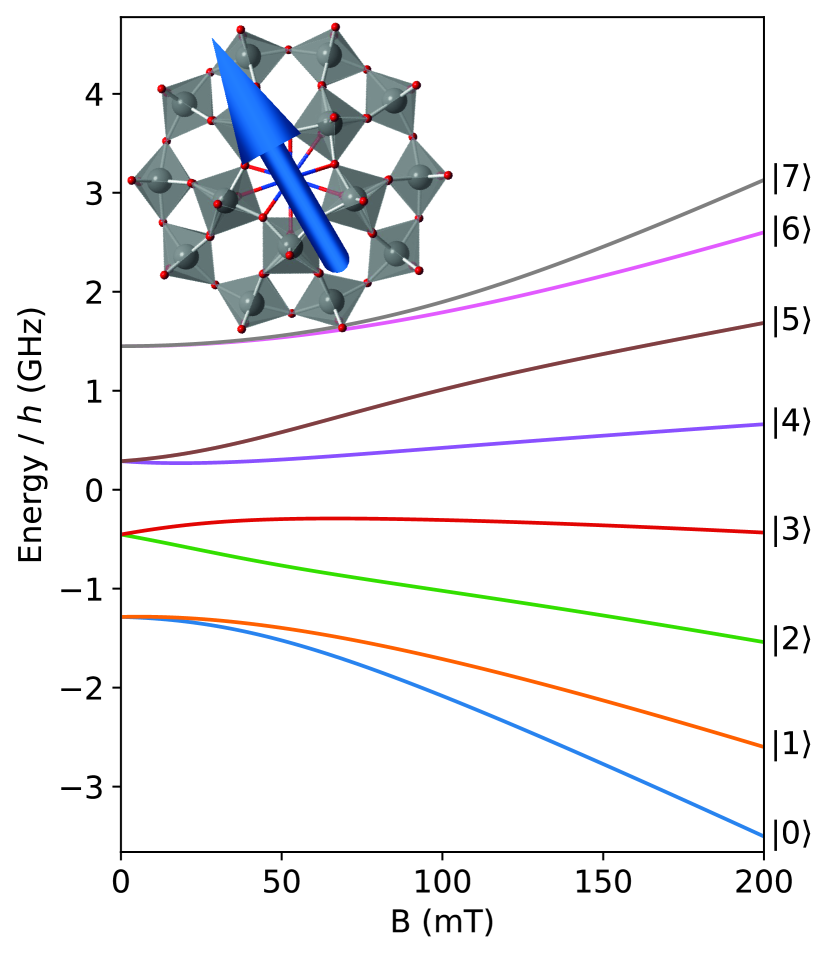
Figure 1: Scheme of the $8$ spin energy levels of the GdW₃₀ complex, whose molecular structure is shown in the inset, for a DC magnetic field applied along its medium anisotropy axis $x$.

In the presence of an environment, the dynamics of the system can be modeled using Lindblad’s equation [30, 31]:

$$\dot{\rho}=\mathcal{L}\rho=-i\left[{\cal H}_{0},\rho\right]+\sum_{\alpha}\gamma_{\alpha}\left(L_{\alpha}\rho L_{\alpha}^{\dagger}-\frac{1}{2}\{L_{\alpha}^{\dagger}L_{\alpha},\rho\}\right)$$ (3)

The dissipative term is therefore defined by a set of Lindblad operators $L_{\alpha}$, each of them associated to a decoherence rate $\gamma_{\alpha}$. For the spin qudits that we are considering, pure dephasing is the dominant decoherence effect [32]. Therefore, we have limited our numerical experiments to the case in which the only nonzero Lindblad operators are $L_{\phi}^{n}=\ket{n}\bra{n}$, all of them associated to the same dephasing constant $\gamma_{\phi}=1/T_{2}$. The latter condition agrees with the results of spin-echo experiments performed on crystals of GdW₃₀ diluted in diamagnetic YW₃₀, which show that $T_{2}$ is nearly the same for all resonant transitions [27].

The model described by Eqs.(1) and (3) includes no external driving. Let us hereafter assume that we add some extra time-dependent term to ${\cal H}_{0}$, so that the total spin Hamiltonian becomes:

$${\cal H}(t)={\cal H}_{0}+f(t)V,$$ (4)

where $V$ describes the interaction mechanism between the control electronics and the molecule, and $f(t)$ is the temporal shape of the drive signal. In the following, we use a time-dependent magnetic field oriented along the easy anisotropy axis $y$ (thus perpendicular to the static one), i.e. $V=-g\mu_{\text{B}}S_{y}$.

The external control drive is designed through the function $f(t)$ of Eq. (4). Different approaches to the control of the system boil down to choosing different functional shapes of $f(t)$. Coherent control of quantum devices is typically implemented by applying sequences of monochromatic pulses, each one addressing the transition between two levels. The result of these pulses is most conveniently pictured as rotations in the Bloch sphere defined in each two-level subspace. A generic rotation (which is a unitary operation) can be parameterized as:

$$R^{(jk)}_{\vec{n}}(\theta)=\exp\left(-i\frac{\theta}{2}\vec{n}\vec{\sigma}^{(jk)}\right)$$ (5)

Here, $\vec{\sigma}^{(jk)}$ is the vector of Pauli matrices within the subspace spanned by the two levels $(jk)$ – in the basis of eigenstates of the control-free Hamiltonian ${\cal H}_{0}$. The unit vector $\vec{n}$ determines the rotation axis and $\theta$ is the rotation angle.

In the interaction representation , this unitary operation can be approximated via the application of a pulse in the form:

$$f(t)=A\Pi_{0}^{t_{f}}(t)\cos(\omega_{jk}t+\phi),$$ (6)

where $\Pi_{t_{a}}^{t_{b}}(t)$ is a square envelope in the interval $(t_{a},t_{b})$ and $\omega_{jk}=|E_{k}-E_{j}|/\hbar$. The amplitude $A$ must be chosen in combination with $t_{f}$, such that:

$$At_{f}=\frac{\theta}{|\langle j|V|k\rangle|}$$ (7)

It is clear from this equation that, the larger the amplitude $A$, the shorter the duration $t_{f}$ that is required to complete the rotation. Finally, in order to have a rotation around the $\vec{n}$ direction, the phase $\phi$ must be chosen such that:

$$\vec{n}=(\cos(\phi-\arg\langle j|V|k\rangle),\sin(\phi-\arg\langle j|V|k\rangle),0)$$ (8)

Rotations around the $z$ axis cannot be directly realized in this way, but they can be built through the composition of three rotations around the $x$ and $y$ axes:

$$R_{Z}(\theta)=R_{X}(\pi/2)R_{Y}(\theta)R_{X}(-\pi/2)$$ (9)

In general, any unitary operation can be decomposed into a sequence of rotations: for any target unitary $U_{\rm target}$, one can always find a set of rotations such that:

$$U_{\rm target}=R^{(j_{r}k_{r})}_{\vec{n}_{r}}(\theta_{r})\dots R^{(j_{2}k_{2})}_{\vec{n}_{2}}(\theta_{2})R^{(j_{1}k_{1})}_{\vec{n}_{1}}(\theta_{1})\,,$$ (10)

modulo a global unimportant phase factor. In order to implement this, one can then define a control waveform consisting of a sequence of the monochromatic single pulses defined above. If the amplitude $A$ for all the pulses in the sequence is the same, fixed by experimental limitations, then it must be related to the total duration of the sequence $T$ by the relation:

$$AT=\sum_{i=1}^{r}\frac{\theta_{i}}{|\langle j_{i}|V|k_{i}\rangle|}\,.$$ (11)

It is clear how one may then concatenate multiple monochromatic single pulses that implement any given unitary operation. This can be done by fixing either the total duration $T$ or the amplitude $A$.

Note, however, that even in the absence of decoherence the resulting operation will not exactly match $U_{\rm target}$: the previous discussion relies on the RWA and on the absence of leakage to other levels during each two-level operation. Reducing this error requires that all transition frequencies are sufficiently different to each other, and that the amplitude $A$ is low enough to make the RWA hold: this approximation becomes exact only in the limit of vanishing amplitude – and, therefore, infinitely long durations. The constructed operation will then differ from the target unitary, and the difference will be larger if shorter durations are demanded.

This sets a limit on the operation speeds that can be implemented by concatenating monochromatic pulses: one cannot simply increase the amplitude $A$ (even if it were experimentally possible) in order to reduce the operation times, since the error due to the approximate nature of the expressions above would then increase. To minimize this error, one should use low amplitudes and long operation times. But then, the system becomes more prone to the errors caused by decoherence. It is clear how the two kinds of error cannot be simultaneously minimized. One must find a compromise amplitude, which may or may not lead to an acceptable fidelity in the operation depending on the level of noise, system characteristics, etc.

The above discussion justifies searching for an alternative to decomposing the unitary into rotations implemented by monochromatic pulse sequences: one may then think of creating the target unitary with a complex multi-frequency pulse tailored with QOCT. In [23], we tried this route using an optimization procedure that did not account for decoherence. In the next sections, we describe how this methodology can be improved by including it.

III Quantum Optimal Control Theory for Open Systems

In this section, we describe the mathematical procedure that applies QOCT to a system coupled to a dephasing bath in order to realize a given target gate $U_{\rm target}$. The application of QOCT to open quantum system was reviewed by Koch [34]. See for example [35, 36] for early applications of this method for the purpose of creating unitary operations in the presence of decoherence. The scheme outlined here, based on Eqs. (25) and (26), permits to use general parametrizations of the control functions – in contrast to the more common real-time representation used by many approaches. This facilitates the enforcement of experimental constraints, as we will show below.

First, we define a functional form for the control pulse $f=f(u,t)$, determined by a set of control parameters $\{u_{k}\}\equiv u$. The time-dependent spin Hamiltonian (4) is then rewritten as:

$${\cal H}(u,t)={\cal H}_{0}+f(u,t)V\,.$$ (12)

The parameterized form of the control functions that we use is:

$$f(u,t)=\Phi(\tilde{f}(u,t))\,,$$ (13)

where $\tilde{f}$ is the Fourier expansion

$$\tilde{f}(u,t)=\sum_{m=1}^{M}\left(u_{2m}\cos(\omega_{m}t)+u_{2m-1}\sin(\omega_{m}t)\right)\,.$$ (14)

Here $\omega_{m}=\frac{2\pi}{T}m$ $M$ sets a cutoff frequency $\omega_{\text{max}}$ that can be chosen according to the sampling rate of the waveform generator. In order to bound the amplitude of the signal, this expansion is modulated by a function $\Phi$ leading to:

$$|f(u,t)|\leq\kappa\quad\textrm{ at any {\hbox{t}}.}$$ (15)

There exist different choices for $\Phi$ that can fulfill this condition. The main requirements for it are: (1) for $|x|\ll\kappa$, $\Phi(x)\approx x$ so that, for low amplitudes, the Fourier series is not altered; (2) as $|x|$ approaches $\kappa$ the function should smoothly evolve towards $\Phi(x)=\kappa$ (or $\Phi(x)=-\kappa$ if $x<0$). The function that we have used here is:

$$\Phi(x) =\textrm{sgn}(x)(1-\sigma(|x|-\kappa))|x|+\kappa\sigma(|x|-\kappa)\,,$$ (16)

$$\sigma(x) =\frac{1}{1+e^{-x}}\,,\;\textrm{(the \emph{sigmoid} function)}.$$ (17)

This modulation will slightly distort the original frequency spectrum of $\tilde{f}$, and in particular it may lead to a violation of the frequency bound $\omega_{\text{max}}$. In any case, this parameterization approximately guarantees that both bandwidth and amplitude limits are set for the control field. Note that most applications of QOCT do not employ parameterized forms of the control functions, but rather work with the full real-time representation of the function (one may say that the parameters are directly the values of the function at the discretized time grid used for the calculations). Although there are also ways to constrain frequencies or amplitudes when using such real-time formulations, using parameterized forms like the one used here is more effective.

In what follows, we describe how we have employed QOCT to find the optimal shape $f(u,t)$ for the control of a spin qudit subject to decoherence. Given a choice of parameters $u$, the system departs from $\rho_{0}$ and evolves into $\rho(u,T)$, following Lindblad’s equation:

$$\dot{\rho}=\mathcal{L}(u,t)\rho\,,$$ (18)

where, as compared to Eq. (3), the dependency of the Lindbladian on the control parameters $u$ and on time has now been made explicit.

Any formulation of QOCT must define a merit function for the system evolution. Let us consider first a simpler problem than the one that we really need to solve: say that we want to find a pulse shape that drives the system from an initial pure state $\rho_{0}=|\psi_{0}\rangle\langle\psi_{0}|$ to an also pure final state $\rho_{\rm target}=|\psi_{\rm target}\rangle\langle\psi_{\rm target}|$. In this case we can use a simple merit function:

$$F(\rho)=\text{Tr}\left[\rho\cdot\rho_{\rm target}\right]\,,$$ (19)

This function has a maximum of one at $\rho=\rho_{\rm target}$. The problem then boils down to the maximization of the following function:

$$G(u)=F(\rho(u,T))\,,$$ (20)

where $T$ is the total propagation time, over all sets of parameters $u$. Despite some caveats related to the state purity [36], this function provides a good measure of the fidelity between the propagated state and the target. In order to compute $G(u)$, one must perform the numerical propagation $\rho_{0}\to\rho(u,T)$. One can then use any of the many available optimization algorithms that do not require the gradient of the function (gradient-free). However, and specially since the number of parameters $u$ can be large, the search is more efficient if one uses a gradient-based algorithm. Using QOCT [37, 38], one may then derive the following expression for the gradient:

$$\frac{\partial G}{\partial u_{m}}(u)=2\int_{0}^{T}\!\!\!{\rm d}t\;\frac{\partial f}{\partial u_{m}}(u,t){\rm Tr}\left(\lambda^{\dagger}(u,t)\big{[}\hat{V},\rho(u,t)\big{]}\right)$$ (21)

In this equation, the costate or adjoint state $\lambda$ is defined by:

$$\left\{\begin{array}[]{l}\dot{\lambda}(u,t)=-\mathcal{L}^{\dagger}(u,t)\lambda(u,t)\,,\\ \lambda(u,T)=\frac{1}{2}\rho_{\rm target}\,.\end{array}\right.$$ (22)

Numerically, the computation of the gradient using this expression requires (1) solving the system equation of motion (Lindblad’s equation) for the state $\rho(u,t)$; (2) solving the previous equation of motion for the costate $\lambda(u,t)$; and (3) computing the integral (21).

However, the problem that we want to solve is more involved than merely finding a pulse that executes the operation $\rho_{0}\rightarrow\rho_{\rm target}$ for a certain state $\rho_{0}$. What we actually want to do is to implement a unitary operation $U_{\rm target}$. The pulse should then map $\rho\rightarrow U_{\rm target}\rho U_{\rm target}^{\dagger}$ for any possible initial state $\rho$. For this purpose, a more complex target function is needed. We take a set of states $\{\rho_{k}\}_{k=1}^{N}$ (ideally it should be a full basis), and define a target function that averages over the effect of the pulse on all those states:

$$G(u)=\frac{1}{\sum_{k}^{N}\Tr\left[\rho_{k}^{2}\right]}\sum_{k}^{N}\Tr\left[\rho_{k}(u,T)\rho_{k}^{\text{target}}\right]\,,$$ (23)

where

$$\rho_{k}^{\text{target}}=U_{\text{target}}\rho_{k}U_{\text{target}}^{\dagger}\,.$$ (24)

As this is just an average over fidelities like the one defined in (20), the gradient equation is trivially extended from Eq. (21):

$$\frac{\partial G}{\partial u_{m}}(u)=2\sum_{k=1}^{N}\int_{0}^{T}\!\!{\rm d}t\;\frac{\partial f}{\partial u_{m}}(u,t){\rm Tr}\left(\lambda_{k}^{\dagger}(u,t)\big{[}\hat{V},\rho_{k}(u,t)\big{]}\right)\,,$$ (25)

where

$$\left\{\begin{array}[]{l}\dot{\lambda}_{k}(u,t)=-\mathcal{L}^{\dagger}(u,t)\lambda_{k}(u,t)\,,\\ \lambda_{k}(u,T)=\frac{1}{2}\rho_{k}^{\rm target}\,.\end{array}\right.$$ (26)

The computation of this gradient is, however, more costly than Eq. (21), as it requires $2N$ propagations: $N$ for the states $\rho_{k}(u,t)$, and $N$ for the corresponding costates $\lambda_{k}(u,t)$. In principle $N=d^{2}$, the Liouville space dimension. Fortunately, as shown in [36], it is sufficient to define the fidelity using a minimum of three states. Here, we have adopted an alternative definition suggested in the same work, which is given in terms of $d+1$ states. These are the $d$ diagonal states $\{\rho_{k}=\ket{k}\bra{k}\}_{k=0}^{d-1}$, which account for the proper mapping of populations, plus an additional state $\rho_{d}$ defined as $(\rho_{d})_{ij}=1/d$, that permits to properly track the phases. This choice substantially reduces the computational cost of the optimization.

The method described above has been implemented in the qocttools code [38].

IV Results

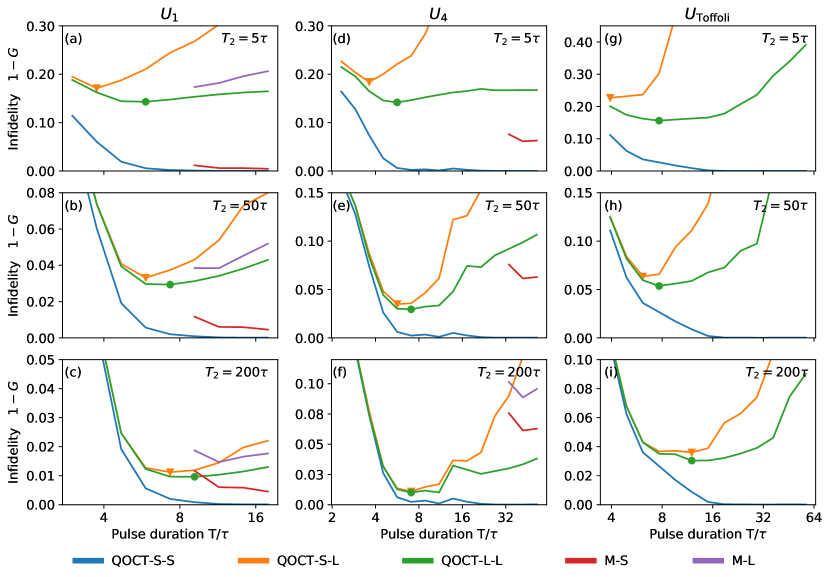
Figure 2: Infidelity of gate operations as a function of the total waveform length, for gates (a-c) $U_{1}$, (d-f) $U_{4}$ and (g-i) $U_{\text{Toffoli}}$. From top to bottom, the simulations use dephasing times of $T_{2}=5\tau,~{}50\tau~{}\text{and}~{}200\tau$ (inset). The results of monochromatic sequences start at longer durations because the amplitude constrain sets a minimum pulse length. The curves that are not displayed have larger durations or infidelities and are of less interest. The orange and green markers indicate the numerical minima of the QOCT-S-L and QOCT-L-L curves, respectively, indicating the best performance achieved with both methods in every case.

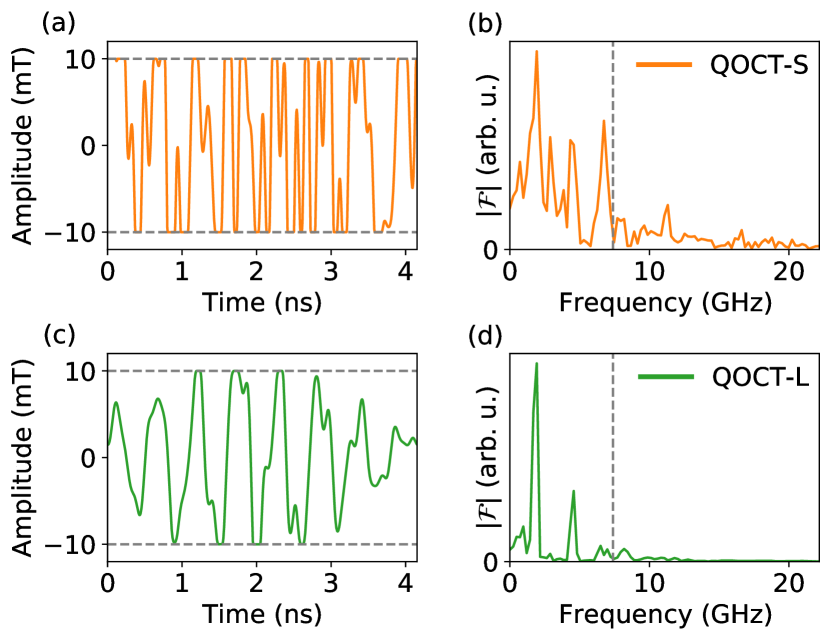
Figure 3: Pulses and their Fourier transforms obtained for the Toffoli gate with $T_{2}=50\tau$ and $T\approx 7.68\tau$ using methods (a, b) QOCT-S, (c, d) QOCT-L. The grey dashed lines indicate the amplitude and frequency bounds set for the optimization.

We apply the method described in the previous section to find pulses that implement, in the GdW₃₀ system, a given target unitary, in the presence of dephasing noise. We set a static magnetic field of $B=150~{}\text{mT}$, and set the following constraints for the pulses: a maximum frequency of $\omega_{\text{max}}=4\omega_{67}$, where $\omega_{67}$ is the transition frequency between the levels 6 and 7, and a maximum amplitude $A_{\rm max}=10\text{ mT}$. We encode three qubits in the 8 energy levels of the spin ($\ket{0}\equiv\ket{000},~{}\ket{1}\equiv\ket{001},\dots,~{}\ket{7}\equiv\ket{111}$) and choose the Toffoli gate as the target unitary, using qubits 1 and 2 as control and qubit 3 as target. In order to realize this operation using a sequence of monochromatic pulses, one would need to decompose it as a product of $8$ rotations: one $\pi$ rotation between levels $\ket{6}=\ket{110}$ and $\ket{7}=\ket{111}$, plus phase gates ($R_{Z}$) on all pairs of two adjacent levels:

$$U_{\rm Toffoli}=e^{i\frac{\pi}{8}} R_{Z}^{(01)}(\frac{1}{4}\pi)R_{Z}^{(12)}(\frac{1}{2}\pi)R_{Z}^{(23)}(\frac{3}{4}\pi)R_{Z}^{(34)}(\pi)$$

$$R_{Z}^{(45)}(\frac{5}{4}\pi)R_{Z}^{(56)}(\frac{3}{2}\pi)R_{Z}^{(67)}(\frac{3}{4}\pi)R_{X}^{(67)}(\pi)$$ (27)

Notice, however, that the last seven rotations around the $Z$ axis have to be implemented as a product of three $X$ and $Y$ rotations, as discussed above in Eq. (9). Therefore, the complete sequence consists of $22$ rotations, i.e. $22$ monochromatic pulses, even for a gate this simple. This makes the total duration very large, and lets decoherence come into play. Below, we will compare the performance of this method based on the decomposition of the unitary into rotations and the use of monochromatic pulses, with the methods based on optimized multifrequency pulses, QOCT-S and QOCT-L. In addition to using the “full” Toffoli gate, and for the sake of observing how the use of QOCT becomes more and more useful as the complexity of a gate grows (in terms of number of necessary rotations), we have also considered shorter sequences, using the first rotations that enter the above definition of the Toffoli gate:

$$U_{1} =R_{Z}^{(67)}(\frac{3}{4}\pi)$$ (28)

$$U_{4} =R_{Z}^{(67)}(\frac{3}{4}\pi)R_{X}^{(67)}(\pi)$$ (29)

After decomposing each $Z$ rotation into three $X$ and $Y$ rotations, $U_{1}$, $U_{4}$ require $1$ and $4$ monochromatic pulses, respectively.

We have then followed the following computational protocol:

1. For a series of predefined times $T$, we implement the target unitary as a sequence of monochromatic pulses, and compute the resulting fidelity using the merit function defined by Eq. (23), in the absence of decoherence. Even then, the fidelity is not one, as there is an error due to leakage and the RWA. This error should decrease with lower amplitudes, and thus larger $T$ according to Eq. (11). From this equation we also deduce that there is a minimum duration time, given by:

   $$T_{\rm min}=\frac{1}{A_{\rm max}}\sum_{i=1}^{r}\frac{\theta_{i}}{|\langle j_{i}|V|k_{i}\rangle|}\,.$$ (30)

   We label these results obtained with monochromatic sequences and Schrödinger’s equation as “M-S”.

2. We then compute the corresponding operation fidelities obtained by those monochromatic sequences in the presence of decoherence, using Lindblad’s equation. We label these results as “M-L”.

3. Next, we apply QOCT to Schrödinger’s equation to obtain an optimized pulse with the parameterization explained above, with the amplitude and frequency bounds $A_{\rm max}$ and $\omega_{\text{max}}$. We label these results as “QOCT-S-S”.

4. We then test the performance of the pulses optimized in the previous step, this time in the presence of decoherence, by solving the dynamics given by Lindblad’s equation for those control waveforms. We label these results as “QOCT-S-L”.

5. Finally, we apply QOCT to Lindblad’s equation as described above, to obtain optimized pulses with the same durations and amplitude and frequency bounds. We label these results as “QOCT-L-L”.

We use the Larmor period of the 6-7 transition $\tau=\frac{2\pi}{\omega_{67}}$ as the unit of time. We consider, for each target unitary, several values of $T_{2}$ ranging from $5\tau$ to $200\tau$. Fig. 2 displays the results obtained for the gates $U_{1}$, $U_{4}$ and $U_{\text{Toffoli}}$ gates, where we quantify the infidelity of the operations, $1-G$, using $G$ given by Eq. (23) as a measure of the fidelity.

Let us focus first on the simplest gate $U_{1}$, consisting of only one rotation (left column). The red line (M-S) displays infidelities obtained with the monochromatic sequences in the absence of decoherence. Those lines start at a duration given by $T_{\rm min}$ in Eq. (30). These infidelities are not zero, but decay to zero as the total duration times $T$ grow. In the presence of dephasing (M-L, purple line), however, the error grows as $T$ becomes longer.

Using the QOCT-S-S method, one obtains the curves shown in blue. In this case the infidelities decay to zero with increasing $T$ much faster than those obtained with monochromatic sequences. This proves how the multi-frequency waveforms can significantly shorten the pulses necessary to produce a given unitary, even for a single rotation, as demonstrated in [23]. If one then tests those optimized pulses in the presence of decoherence (QOCT-S-L, orange curves), the errors grow as expected. We observe a minimum in the curve (indicated with a marker), a maximum-fidelity sweet spot where neither control nor decoherence errors are dominant with respect to each other. This is precisely the compromise mentioned above, attained when simultaneously minimizing the two different errors that are present in the process.

The results obtained from QOCT-L-L (green curves) are the best in the presence of decoherence. The difference with respect to the QOCT-S-L fidelities is larger at longer durations $T$, and becomes negligible at small $T$. This is not surprising, since QOCT-S and QOCT-L are only effectively different if decoherence is relevant, i.e. for large durations. For the same reason, the QOCT-L method is significantly better for smaller $T_{2}$ (top panel), whereas the difference is smaller at larger $T_{2}$ (bottom panel), i.e. if the dephasing becomes weaker. The QOCT-L curves also have a sweet spot, for the same reasons as before. This minimum infidelity is lower than the one in the QOCT-S-L curve, which shows how the QOCT-L-L procedure helps to obtain the pulse with the minimum possible error.

As the complexity of the target unitary increases, from $U_{1}$ to $U_{4}$ and then to $U_{\text{Toffoli}}$, we observe several effects. First of all, the minimum duration required for the monochromatic sequences grows (as more rotations are needed): notice how for the $U_{4}$ gate (middle column), the M-S and M-L curves start at long durations – and we do not even show them in the $U_{\text{Toffoli}}$ case (right column), as $T_{\rm min}$ is too high. At those long durations, the decoherence error (difference between M-S and M-L) is quite high – for this reason, we only show the M-L curve for $U_{4}$ in the $T_{2}=200\tau$ case, as for the other cases the M-L curve shows too large infidelities.

QOCT-S-S outperforms M-S by a larger difference as compared to the $U_{1}$ case: the infidelity decays much earlier to zero. The difference between QOCT-S-L and QOCT-L-L also becomes larger as the complexity of the gate grows. These are all consequences of the longer durations that are necessary to implement the operations. As a final comment regarding Fig. 2: notice how the QOCT curves are not very smooth; the reason is that the algorithm may not necessarily find the global optimum. This difficulty probably grows with increasing gate complexity.

Fig. 3 shows some of the control pulses obtained with QOCT, together with the absolute value of their Fourier transforms, computed for the Toffoli gate, using $T_{2}=50\tau$ and $T\approx 7.68\tau$. Panels (a) and (b) display the pulse obtained with QOCT-S, whereas panels (c) and (d) display the pulse obtained with QOCT-L. One can see how the designed parametrization of the pulses fixes the maximum amplitude for both pulses, that cannot surpass 10 mT. The frequency spectrum, however, presents small contributions beyond the frequency cutoff. These are not present in the Fourier parameterization $\tilde{f}$, but appear in the final pulse $f$ because of the effect of the modulation function $\Phi$, as anticipated above.

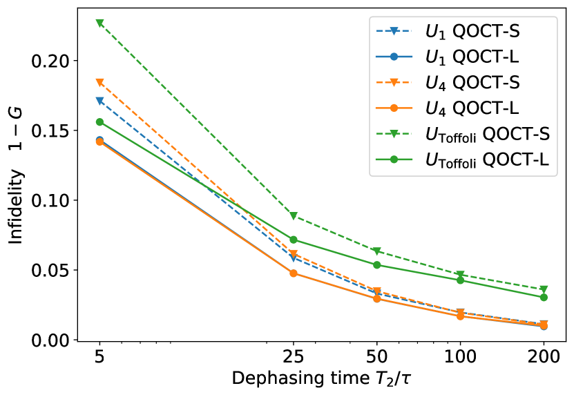
Figure 4: Minimum infidelities achieved by the QOCT-S (triangle marker, dashed lines) and QOCT-L (circular marker, solid lines) methods for all three target unitaries, as a function of the dephasing time $T_{2}$. The lines are guides to the eye.

Finally, Fig. 4 shows the minimum infidelities achieved for each gate using the QOCT-S and QOCT-L methods, as a function of $T_{2}$. This plot summarizes the previous results, as it shows the best possible pulse that can be obtained with each method. It can be seen how, when the dephasing is weak (long $T_{2}$), both methods perform comparably well. However, in the presence of strong dephasing, the QOCT-L method achieves substantially lower errors. This difference also increases with the complexity of the target unitary.

V Conclusions and Outlook

This work investigates the use of QOCT for open quantum systems to find pulses capable of implementing operations in molecular nanomagnets subject to strong dephasing. Our results show that accounting for decoherence when numerically designing control pulses makes a significant difference. Monochromatic pulse sequences show a bad performance in the presence of pure dephasing, and so do the waveforms optimized using QOCT on top of Schrödinger’s equation. However, modelling dephasing using Lindblad’s master equation and applying QOCT to it yields higher gate fidelities. The difference is larger the shorter the coherence times and the more complex the target operations.

This tool is useful for two reasons. First, it allows one to give a realistic numerical bound to the achievable gate fidelities on these systems, in the presence of dephasing and accounting for the amplitude and sampling-rate limitations of the instrumentation. And second, it finds the optimal waveforms for this purpose, outperforming the other approaches.

We consider extending this method in several directions. First, one could add amplitude damping ($T_{1}$) to the model, to better account for all possible sources of errors. Although we do not expect any significant differences in the case of our platform, in which dephasing is orders of magnitude stronger, this could be useful in other circumstances. Second, we also consider the use of more realistic master equations – for example, employing time-dependent Lindblad operators. We have ignored this possibiligy so far because, up to first order of approximation, the dissipative operators are independent of the drive, and therefore invariant in time. However, the use of large amplitudes and short pulses may imply a regime where second and higher order terms are not negligible, and there is a relevant time-dependent contribution to the dissipator.