Phase estimation via coherent and photon-catalyzed squeezed vacuum states

Abstract

The research focused on enhancing the measurement accuracy through the use of non-Gaussian states has garnered increasing attention. In this study, we propose a scheme to input the coherent state mixed with photon-catalyzed squeezed vacuum state into the Mach-Zender interferometer to enhance phase measurement accuracy. The findings demonstrate that photon catalysis, particularly multi-photon catalysis, can effectively improve the phase sensitivity of parity detection and the quantum Fisher information. Moreover, the situation of photon losses in practical measurement was studied. The results indicate that external dissipation has a greater influence on phase sensitivity than the internal dissipation. Compared to input coherent state mixed with squeezed vacuum state, the utilization of coherent state mixed photon-catalyzed squeezed vacuum state, particularly the mixed multi-photon catalyzed squeezed vacuum state as input, can enhance the phase sensitivity and quantum Fisher information. Furthermore, the phase measurement accuracy can exceed the standard quantum limit, and even surpass the Heisenberg limit. This research is expected to significantly contribute to quantum precision measurement.

PACS: 03.67.-a, 05.30.-d, 42.50,Dv, 03.65.Wj

I Introduction

With the advancement of science and technology, quantum metrology, which utilizes non-classical quantum states to achieve high-precision measurement, has been extensively applied [1, 2, 3, 4, 5, 6, 7, 8, 9, 10]. The Mach-Zehnder interferometer (MZI) is widely used as a measurement instrument in quantum precision measurement [11, 12, 13, 14]. In 1981, Caves proposed a scheme involving the mixture of coherent state (CS) and squeezed vacuum state (SVS) as the input state of MZI and found that the measurement accuracy can exceed the standard quantum limit (SQL) $\Delta\varphi=1/\sqrt{\bar{N}}$, where $\bar{N}$ represents the total average photon number of the input state [15]. Subsequently, the three main parts of quantum precision measurement, namely, the preparation of input states, the interaction between the input state and the system under consideration, and the detection of the output state [16, 17], have gained significant attention. Currently, numerous quantum states such as the NOON state, twin-Fock state, and two-mode squeezed vacuum (TMSV) state inputs have been investigated and proven to surpass the SQL and even achieve the Heisenberg limit (HL) $\Delta\varphi=1/\bar{N}$ [18, 19, 20, 21, 22, 23, 24, 25, 26, 27, 28, 29, 30, 31, 32]. In terms of the detection method, parity detection offers significant advantages in improving measurement accuracy. In 2011, Seshadreesan et al. demonstrated that by inputting the CS mixed with SVS into MZI and utilizing parity detection, the phase sensitivity can reach the HL [33].

Recent studies have shown that enhancing the non-classical properties of quantum states through non-Gaussian operations is beneficial for improving measurement accuracy [34, 35, 36, 37, 38, 39, 40, 41, 42, 43, 44]. Non-Gaussian operations such as photon subtraction, addition, and catalysis can be simulated with optical beam splitters. Jia et al. conducted a detailed study of the non-classical properties of the non-Gaussian state prepared through such non-Gaussian operations on the SVS [45]. Their findings indicate that photon-subtracted, photon-added, and photon-catalyzed non-Gaussian operations can effectively enhance the non-classical properties of quantum states. Utilizing coherent state mixed with photon-subtracted (-added) SVS (PSSVS/PASVS) as input in MZI for quantum precision measurement has demonstrated effective enhancements [38, 39]. Furthermore, given the inevitable photon losses during actual measurement, increasing attention has been devoted to understanding the impact of photon losses on measurement accuracy, which holds great significance for quantum precision measurement applications. Building on the insights from previous research, we propose employing the CS mixed with photon-catalyzed SVS (PCSVS) as the input state of MZI. We consider the phase sensitivity and quantum Fisher information (QFI) under ideal and photon-loss conditions to develop an improved phase measurement accuracy scheme. It is demonstrate that our scheme can significantly enhance phase estimation, particularly in the context of multi-photon catalysis, leading to measurement accuracy exceeding the SQL or even reaching the HL.

The organization of this paper is as follows: In Sec. II, we initially introduce the preparation process and fundamental properties of the PCSVS. In Sec. III, we investigate the phase sensitivity with parity measurement and the QFI in ideal circumstances. Sec. IV further examines the impact of photon losses on the phase sensitivity, including external and internal dissipations. In Sec. V, we explore the influence of photon losses on the QFI. The last section provides a summary of the main results.

II Photon-catalyzed squeezed vacuum state

Fig. 1 illustrates the input of the SVS in mode $b$ and the Fock state $\left|m\right\rangle_{c}$ in mode $c$ into the two ports of the beamsplitter (BS0) with transmissivity $\eta$. Subsequently, the photon detector at the output port of mode $c$ detects the Fock state $\left|m\right\rangle_{c}$ with the identical photon number $m$, thereby leading to the successful preparation of the PCSVS at the other output port of mode $b$. According to Ref. [45], the equivalent operator for the $m$-photon catalysis operation can be defined as

$$\hat{O}_{m} = \left.{}_{c}\left\langle m\right|B\left(\eta\right)\left|m\right\rangle_{c}\right.$$ (1)

$$= \left.\frac{\left(\sqrt{\eta}\right)^{b^{\dagger}b+m}}{m!}\frac{\partial^{m}}{\partial\tau^{m}}\frac{1}{1-\tau}\left(\frac{1-\tau/\eta}{1-\tau}\right)^{b^{\dagger}b}\right|_{\tau=0},$$

where $B\left(\eta\right)=\exp\left[\left(b^{\dagger}c-bc^{\dagger}\right)\arccos\sqrt{\eta}\right]$ is the BS0 operator. Consequently, the expression of the PCSVS can be derived as

$$\left|\psi_{PCSVS}\right\rangle_{b} = \frac{\hat{O}_{m}}{\sqrt{P_{m}}}S\left(r\right)\left|0\right\rangle_{b}$$ (2)

$$= \left.\frac{W_{0}}{\sqrt{P_{m}}}\frac{\partial^{m}}{\partial\tau^{m}}\frac{\exp\left(Wb^{\dagger 2}\right)}{1-\tau}\right|_{\tau=0}\left|0\right\rangle_{b},$$

where $W_{0}=\frac{\sqrt{\eta}^{m}}{m!\sqrt{\cosh r}}$, $W=-\frac{\eta\left(1-\tau/\eta\right)^{2}\tanh r}{2\left(1-\tau\right)^{2}}$, $S\left(r\right)\left|0\right\rangle_{b}=\exp\left[r\left(b^{2}-b^{\dagger 2}\right)/2\right]\left|0\right\rangle_{b}$ is the SVS with the squeezing parameter $r$ and $P_{m}$ represents a normalized coefficient, i.e.,

$$P_{m}=\left.W_{0}^{2}\frac{\partial^{2m}}{\partial\tau^{m}\partial\tau_{1}^{m}}\epsilon\left(1-4W_{1}W\right)^{-\frac{1}{2}}\right|_{\tau=\tau_{1}=0},$$ (3)

and

$$W_{1} = -\frac{\eta\left(1-\tau_{1}/\eta\right)^{2}\tanh r}{2\left(1-\tau_{1}\right)^{2}},$$

$$\epsilon = \frac{1}{\left(1-\tau\right)\left(1-\tau_{1}\right)}.$$ (4)

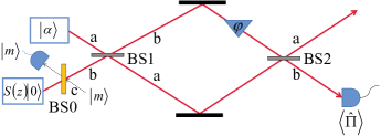
Figure 1: The schematic diagram of the preparation of PCSVS and the parity detection of phase shift when the PCSVS and CS are injected from the two ports of the first beamsplitter BS1 of the MZI under ideal conditions.

The average photon number of an input state, which reflects the energy characteristics of a light field, is a crucial parameter in the investigation of quantum precision measurement. Therefore, we further examine the average photon number of the PCSVS. Using Eq. (2), the average photon number of PCSVS is given by

$$\overline{n}_{b} = \left.{}_{b}\left\langle\psi_{PCSVS}\right|b^{\dagger}b\left|\psi_{PCSVS}\right\rangle_{b}\right.$$ (5)

$$= \hat{D}\frac{\epsilon}{\left(1-4W_{1}W\right)^{\frac{3}{2}}}-1,$$

where

$$\hat{D}=\frac{W_{0}^{2}}{P_{m}}\frac{\partial^{2m}}{\partial\tau^{m}\partial\tau_{1}^{m}}\left\{\cdot\right\}|_{\tau=\tau_{1}=0}.\$$ (6)

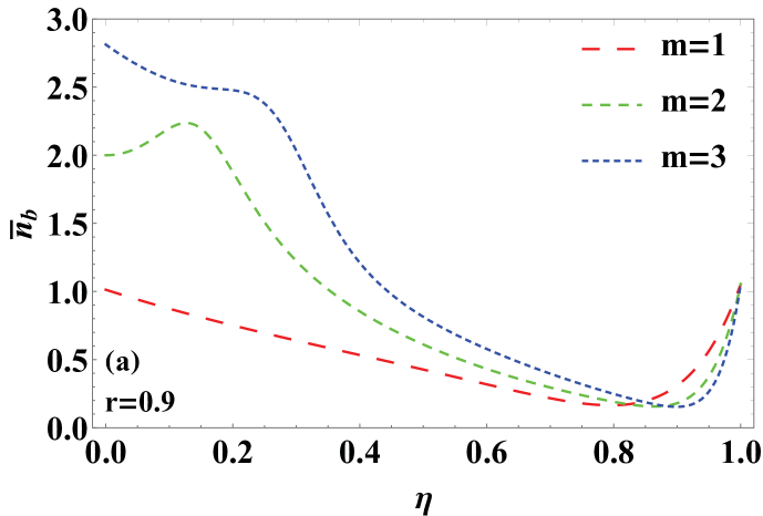
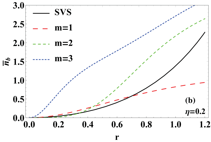
Figure 2: For the catalysis photon numbers $m=1,2,3$, (a) the average photon number $\overline{n}_{b}$ as a function of the transmissivity $\eta$ for a given squeezing parameter $r=0.9$, and (b) $\overline{n}_{b}$ as a function of $r$ for a given $\eta=0.2$ and its comparison with the case of SVS.

In order to comprehensively analyze the relationship between the average photon number and each parameter, for different catalysis photon numbers $m=1,2,3$, Fig. 2 illustrates the variation of the average photon number $\overline{n}_{b}$ of PCSVS with the transmissivity $\eta$ at a fixed squeezing parameter $r=0.9$ (Fig. 2(a)), and the variation of $\overline{n}_{b}$ with $r$ for a given $\eta=0.2$ (Fig. 2(b)). From Fig. 2(a), it is observed that $\overline{n}_{b}$ increases with an increase of the catalysis photon number $m$ when the transmissivity $\eta$ is in the range of $0$ to approximately $0.85$ for a fixed $r=0.9$, whereas $\overline{n}_{b}$ increases with a decrease of $m$ when $\eta$ is in the range of about $0.85$ to $1$. The $\overline{n}_{b}$ corresponding to $\eta=1$ is equal to the average photon number of SVS. A comparison indicates that the $\overline{n}_{b}$ of the multiphoton catalysis SVS (MC-SVS) corresponding to $m\geqslant 2$ is greater than the average photon number of SVS when $\eta$ takes a smaller value. Fig. 2(b) presents the plot of the average photon number of the SVS and the PCSVS at a specific transmissivity $\eta=0.2$ as a function of the squeezing parameter $r$. As demonstrated in Fig. 2(b), at $\eta=0.2$, $\overline{n}_{b}$ rises with $r$, and the $\overline{n}_{b}$ of MC-SVS surpasses that of SVS within a specific range of $r$. Notably, in cases where the squeezing parameter $r$ is relatively small, the average photon number $\overline{n}_{b}$ of the single-photon PCSVS ($m=1$) can also exceed that of SVS.

III Phase estimation of mixing PCSVS with CS based on MZI under ideal conditions

III.1 Phase sensitivity with parity detection

The conventional MZI model, depicted in Fig. 1, primarily comprises two 50:50 beam splitters (BS1 and BS2) with equal transmissivity and reflectivity, two mirrors, and a phase shifter. The beam splitter’s impact on the input state is equivalent to a rotation in theory. Therefore, as demonstrated in Ref. [46], the operators of BS1 and BS2 can be represented using the SU(2) group theory separately in the Schwinger representation as $B_{1}\left(-\pi/2\right)=e^{-i\frac{\pi}{2}J_{1}}$ and $B_{2}\left(\pi/2\right)=e^{i\frac{\pi}{2}J_{1}}$, respectively. In mode $b$ of the MZI, the phase shift of the phase shifter is denoted as $\varphi$, and the phase shifter operator can be defined as $U\left(\varphi\right)=e^{i\varphi b^{\dagger}b}$. The equivalent operator of the MZI can be expressed as

$$U_{MZI}=e^{i\pi J_{1}/2}e^{i\varphi b^{\dagger}b}e^{-i\pi J_{1}/2}=e^{i\varphi J_{0}}e^{-i\varphi J_{2}},$$ (7)

where the Casimir operator $J_{0}$ and the angular momentum operator $J_{i}\left(i=1,2,3\right)$ satisfying the commutation relation $\left[J_{i},J_{j}\right]=i\varepsilon_{ijk}J_{k}\left(i,j,k=1,2,3\right)$ can be represented by the photon annihilation (creation) operators $a,b$ ($a^{\dagger},b^{\dagger}$), as follows

$$J_{0} = \frac{1}{2}\left(a^{{\dagger}}a+b^{{\dagger}}b\right),\ J_{1}=\frac{1}{2}\left(a^{{\dagger}}b+ab^{{\dagger}}\right),$$

$$J_{2} = \frac{1}{2i}\left(a^{{\dagger}}b-ab^{{\dagger}}\right),J_{3}=\frac{1}{2}\left(a^{{\dagger}}a-b^{{\dagger}}b\right),$$ (8)

$\left[J_{0},J_{i}\right]=0$, and $J_{i}$ satisfies $e^{i\frac{\pi}{2}J_{1}}e^{i\varphi J_{3}}e^{-i\frac{\pi}{2}J_{1}}=e^{-i\varphi J_{2}}$. Hence, the output state $\left|out\right\rangle$ obtained from the input of CS mixed with PCSVS in the MZI can be represented as

$$\left|out\right\rangle=U_{MZI}\left|in\right\rangle=e^{i\varphi J_{0}}e^{-i\varphi J_{2}}\left|\alpha\right\rangle_{a}\otimes\left|\psi_{PCSVS}\right\rangle_{b},$$ (9)

where $\left|in\right\rangle$ is the input state, and $\left|\alpha\right\rangle_{a}=\exp[-\left|\alpha\right|^{2}/2+\alpha a^{\dagger}]\left|0\right\rangle_{a}$ is a CS on mode $a$, $\alpha=\left|\alpha\right|e^{i\theta}$.

The parity detection at the output of mode $b$ can be defined as

$$\Pi_{b}=\left(-1\right)^{b^{{\dagger}}b}=e^{i\pi b^{{\dagger}}b}=\int\frac{d^{2}\gamma}{\pi}\left|\gamma\right\rangle_{bb}\left\langle-\gamma\right|,\$$ (10)

where $\left|\gamma\right\rangle_{b}$ is the CS of mode $b$. By utilizing Eq. (9), the average value of parity operator is given by

$$\left\langle\Pi_{b}\right\rangle = \left\langle out\right|\Pi_{b}\left|out\right\rangle$$ (11)

$$= \left\langle in\right|e^{i\varphi J_{2}}e^{-i\varphi J_{0}}\Pi_{b}e^{i\varphi J_{0}}e^{-i\varphi J_{2}}\left|in\right\rangle.$$

As $\left[\Pi_{b},J_{0}\right]=0$, Eq. (11) can be reformulated as

$$\left\langle\Pi_{b}\right\rangle=\left\langle in\right|e^{i\varphi J_{2}}\Pi_{b}e^{-i\varphi J_{2}}\left|in\right\rangle.\$$ (12)

Using the following unitary transformation

$$e^{-i\varphi J_{2}}a^{\dagger}e^{i\varphi J_{2}} = a^{\dagger}\cos\frac{\varphi}{2}+b^{\dagger}\sin\frac{\varphi}{2},\$$

$$\ e^{-i\varphi J_{2}}b^{\dagger}e^{i\varphi J_{2}} = b^{\dagger}\cos\frac{\varphi}{2}-a^{\dagger}\sin\frac{\varphi}{2},$$ (13)

and $e^{-i\varphi J_{2}}\left|00\right\rangle=\left|00\right\rangle$, one has

$$e^{-i\varphi J_{2}}\left|in\right\rangle = \hat{D}^{\prime}\exp\left[-\frac{1}{2}\left|\alpha\right|^{2}+\alpha\left(a^{\dagger}\cos\frac{\varphi}{2}+b^{\dagger}\sin\frac{\varphi}{2}\right)\right.$$ (14)

$$\left.+W\left(b^{\dagger}\cos\frac{\varphi}{2}-a^{\dagger}\sin\frac{\varphi}{2}\right)^{2}\right]\left|00\right\rangle,$$

where $\hat{D}^{\prime}$ is defined as

$$\hat{D}^{\prime}=\frac{W_{0}}{\sqrt{P_{m}}}\frac{\partial^{m}}{\partial\tau^{m}}\frac{1}{1-\tau}\left\{\cdot\right\}_{\tau=0}.\$$ (15)

Using Eqs. (10) and (14), along with the following integral equation [47]

$$\int\frac{d^{2}z}{\pi}e^{\zeta\left|z\right|^{2}+\xi z+\eta z^{\ast}+fz^{2}+gz^{\ast 2}}=\frac{e^{\frac{-\zeta\xi\eta+\xi^{2}g+\eta^{2}f}{\zeta^{2}-4fg}}}{\sqrt{\zeta^{2}-4fg}},$$ (16)

whose convergence conditions Re$\left(\xi\pm f\pm g\right)<0$ and Re$\left(\frac{\zeta^{2}-4fg}{\xi\pm f\pm g}\right)<0$, Eq. (12) can be further calculated as

$$\left\langle\Pi_{b}\right\rangle = \hat{D}\frac{\varepsilon}{\sqrt{1-4W_{1}W\cos^{2}\varphi}}$$ (20)

$$\times\exp\left[\frac{\left(\begin{array}[]{c}\left(1-4W_{1}W\right)\left(\cos\varphi-1\right)\\ -4W_{1}W\sin^{2}\varphi\end{array}\right)\left|\alpha\right|^{2}}{1-4W_{1}W\cos^{2}\varphi}\right]$$

$$\times\exp\left[\frac{\left(W_{1}\alpha^{2}+W\alpha^{\ast 2}\right)\sin^{2}\varphi}{1-4W_{1}W\cos^{2}\varphi}\right].$$

In particular, for the case of $\eta=1$ that the input state is CS mixed with SVS [33], the above equation can be simplified as

$$\left\langle\Pi_{b}\right\rangle = \frac{1}{\sqrt{1+\sinh^{2}r\sin^{2}\varphi}}$$ (21)

$$\times\exp\left[\frac{2\left(\cos\varphi-1-\sinh^{2}r\sin^{2}\varphi\right)\left|\alpha\right|^{2}}{2\left(1+\sinh^{2}r\sin^{2}\varphi\right)}\right.$$

$$\left.-\frac{\sinh 2r\sin^{2}\varphi\text{Re}\left(\alpha^{2}\right)}{2\left(1+\sinh^{2}r\sin^{2}\varphi\right)}\right].$$

Since the phase $\theta=0$ of the CS can achieve better phase sensitivity [33], here we assumes $\alpha=\alpha^{\ast}=\left|\alpha\right|$.

Phase sensitivity is a crucial parameter for phase measurement. Improving phase sensitivity is synonymous with reducing phase uncertainty, leading to increased precision in phase measurement. The phase sensitivity $\Delta\varphi$ with parity detection can be obtained using the average value of the parity operator (Eq. (20)) and the error propagation formula, as shown below:

$$\triangle\varphi=\frac{\triangle\Pi_{b}}{\left|\partial\left\langle\Pi_{b}\right\rangle/\partial\varphi\right|},\$$ (22)

where $\Delta\Pi_{b}=\sqrt{\langle\Pi_{b}^{2}\rangle-\langle\Pi_{b}\rangle^{2}}=\sqrt{1-\langle\Pi_{b}\rangle^{2}}$.

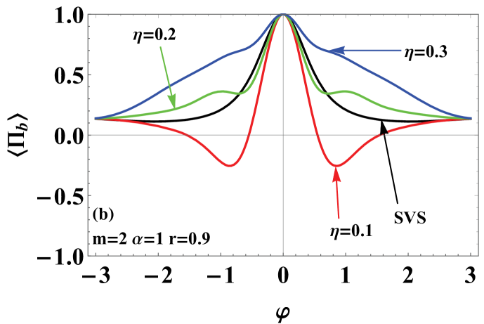
Figure 3: For a fixed coherent amplitude $\alpha=1$ and squeezing parameter $r=0.9$, (a) with transmissitivity $\eta=0.2$ and catalysis photon numbers $m=1,2,3$, and (b) with $m=2$ and $\eta=0.1,0.2,0.3$, the variation of the parity signal $\langle\Pi_{b}\rangle$ with phase shift $\varphi$. The black solid line corresponds to the SVS (without photon catalysis) for comparison.

As depicted in Fig. 3, for a given coherent amplitude $\alpha$ and squeezing parameter $r$, the figure illustrates the variation of the parity signal (average value of the parity operator) with the phase shift $\varphi$. A narrower central peak in the image indicates a higher resolution. In Fig. 3(a), it can be observed that, at a fixed transmissivity $\eta=0.2$ of the BS0, the operation of multiphoton catalysis ($m\geqslant 2$) effectively enhances the resolution of the phase shift compared to that of SVS (without photon catalysis). Meanwhile, Fig. 3(b) illustrates that, in the case of catalysis photon number $m=2$, adjusting $\eta$ can also result in a narrower central peak, thus achieving better phase shift resolution than the input CS mixed with SVS. Therefore, optimizing the parameter $\eta$ is valid for improving the phase sensitivity.

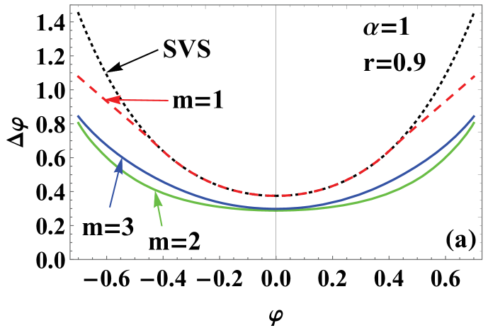
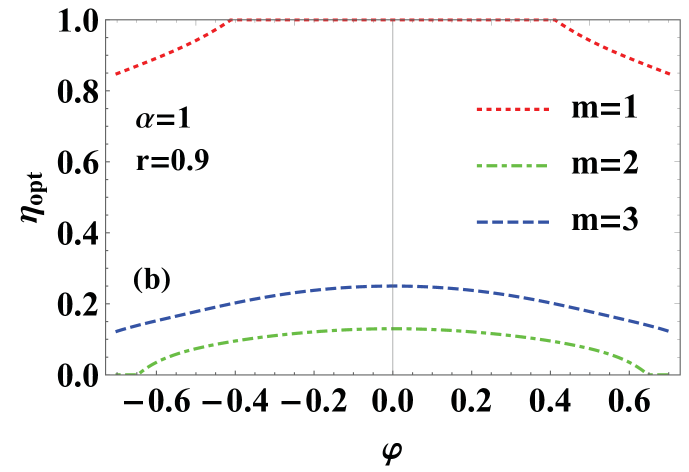
Figure 4: For the catalysis photon numbers $m=1,2,3$, a coherent amplitude $\alpha=1$, and a squeezing parameter $r=0.9$, (a) the variation of phase sensitivity $\Delta\varphi$ with phase shift $\varphi$ for optimized $\eta$ ($\eta_{opt}$), with the black dotted line representing the SVS (without photon catalysis) for comparision, and (b) the variation of $\eta_{opt}$ with $\varphi$.

Fig. 4(a) visually illustrates the variation of phase sensitivity $\Delta\varphi$ with phase shift $\varphi$ for a given coherent amplitude $\alpha=1$, squeezing parameter $r=0.9$, and optimized transmissivity $\eta_{opt}$. It is evident that $\Delta\varphi$ reaches its optimum value at $\varphi=0$. For small $\varphi$ absolute values, the phase sensitivity for the case of catalysis photon number $m=1$ is comparable to that of the CS mixed with SVS input in the MZI. However, as the absolute value of $\varphi$ increases, the phase sensitivity for $m=1$ significantly improves. Furthermore, for the cases of the CS mixed with the MC-SVS with $m=2$ and $3$ as input, the phase sensitivity is notably enhanced. This demonstrates the advantageous impact of photon catalysis operation on improving phase sensitivity with parity detection. Notably, the multiphoton catalysis operation can notably enhance phase sensitivity. To elucidate the value of $\eta_{opt}$, Fig. 4(b) presents the function image of $\eta_{opt}$ changing with $\varphi$. It is apparent that for the case of $m=1$, the optimized transmissivity $\eta_{opt}=1$, equivalent to the input state of mode $b$ being SVS, occurs the value of $\varphi$ between approximately $-0.48$ and $0.48$. Conversely, for $m=2$ and $3$, $\eta_{opt}$ is relatively small.

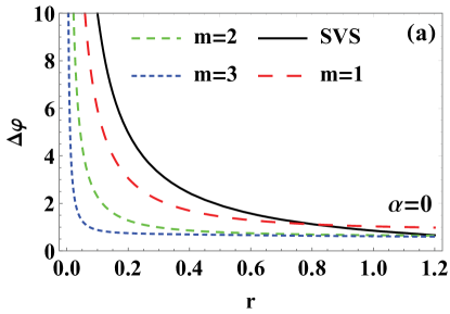
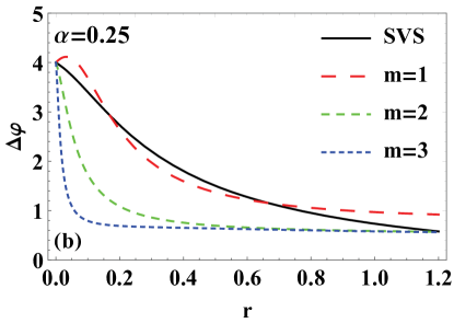
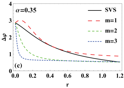
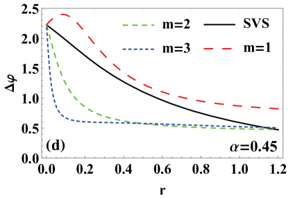
Figure 5: The phase sensitivity $\Delta\varphi$ as a function of the squeezing parameter $r$ for the catalysis photon numbers $m=1,2,3$, fixed the phase shift $\varphi=10^{-4}$, transmissitivity $\eta=0.1$ and fixed the different coherent amplitude (a) $\alpha=0$, (b) $\alpha=0.25$, (c) $\alpha=0.35$, (d) $\alpha=0.45$. The black solid line corresponds to the SVS (without photon catalysis) for comparison.

To clearly see the effects of parameters of the input state on phase sensitivity and compared with the CS and SVS as inputs, we plot the phase sensitivity $\Delta\varphi$ as a function of the squeezing parameter $r$ for a given phase shift $\varphi=10^{-4}$, transmissivity $\eta=0.1$ and fixed the different coherent amplitude $\alpha$, as depicted in Figs. 5(a)-(d). It is found that the phase sensitivity $\Delta\varphi$ can be improved by increasing the value of $r$ across a wide range as well as increasing $\alpha$. Furthermore, as can be seen in Fig. 5(a) and Fig. 5(b), when fixed the small coherent amplitude $\alpha=0,0.25$, for the case of the catalysis photon numbers $m=1,2,3$, particularly for the case of multiphoton catalysis operation with $m=2,3$, the phase sensitivity can be improved more efficiently than the scheme using the CS mixed with SVS as the input state. The relative phase sensitivity to the SVS (without photon catalysis) can be improved within a specific range of lower squeezing parameters for $m=1$. However, it can be seen from Fig. 5(c) and Fig. 5(d) that increasing $\alpha$ to $0.35$ and $0.45$, respectively, leads to a decrease in phase sensitivity for $m=1$ compared to the SVS. Nevertheless, utilizing a CS mixed with the MC-SVS ($m=2,3$) as inputs still yields a significant enhancement in phase sensitivity compared to using the CS mixed with SVS. The preceding discussion leads to the conclusion that selecting smaller values for $\alpha$, $r$, and $\eta$ would enhance the suitability of mixing the CS with PCSVS input MZI, thereby improving phase measurement accuracy compared to input the CS mixed with SVS. Moreover, achieving a smaller coherent amplitude $\alpha$ and squeezing parameter $r$ is relatively more feasible experimentally.

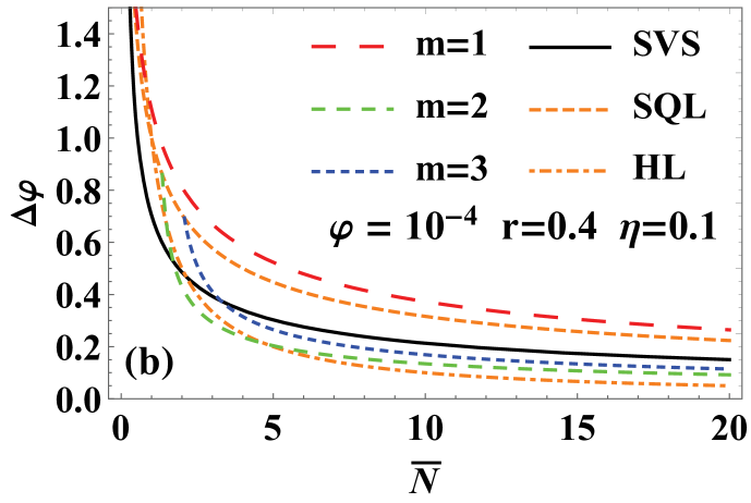
Figure 6: For the catalysis photon numbers $m=1,2,3$, fixed the phase shift $\varphi=10^{-4}$, transmissivity $\eta=0.1$ and squeezing parameter $r=0.4$, (a) the phase sensitivity $\Delta\varphi$ as a function of the coherent amplitude $\alpha$, and (b) $\Delta\varphi$ as a function of the total average photon number $\bar{N}$ comparing with the SQL and the HL. The black solid line corresponds to the SVS (without photon catalysis) for comparison.

In Fig. 6(a), an illustration depicting the change in phase sensitivity $\Delta\varphi$ concerning the coherent amplitude $\alpha$ is provided for the squeezing parameter $r=0.4$. It is apparent that $\Delta\varphi$ improves with the increase of $\alpha$, and $\Delta\varphi$ corresponding to the catalysis photon numbers $m=1,2,3$ surpasses that of the CS mixed with SVS as the input state. Notably, for $m=1$, $\Delta\varphi$ can be improved relative to the case of SVS (without photon catalysis) when $\alpha$ is small, and worse than the case of SVS when $\alpha$ is large. Additionally, Fig. 6(b) investigates the effect of the total average photon number $\bar{N}$ on $\Delta\varphi$. The total average photon number $\bar{N}$ reflects the energy of the input optical field, $\bar{N}=\bar{n}_{a}+\overline{n}_{b}$, where $\bar{n}_{a}=\alpha^{2}$ represents the average photon number of the CS input to the $a$-mode. It is evident from Fig. 6(b) that $\Delta\varphi$ gradually enhances with the increase of $\bar{N}$, and $\Delta\varphi$ of the multi-photon catalysis operation corresponding to $m=2,3$ shows more significant improvement than that of the SVS. Furthermore, in the case of $m=2,3$, $\Delta\varphi$ can surpass the SQL and approach the HL more effectively. Specifically, for $m=2$, $\Delta\varphi$ can exceed the HL in a small range of $\bar{N}$, and the corresponding input resources with lower energy are easier to fabricate experimentally.

III.2 Quantum Fisher Information

The QFI describes the maximum amount of information for measuring the phase shift $\varphi$. When a pure state is input to the MZI, the QFI is caculated as [48]

$$F_{Q}=4\left[\left\langle\psi_{\varphi}^{\prime}|\psi_{\varphi}^{\prime}\right\rangle-\left|\left\langle\psi_{\varphi}^{\prime}|\psi_{\varphi}\right\rangle\right|^{2}\right],$$ (23)

where $\left|\psi_{\varphi}\right\rangle=e^{i\varphi b^{\dagger}b}e^{-i\frac{\pi}{2}J_{1}}\left|in\right\rangle$ is the quantum state before the BS2 of the MZI, and $\left|\psi_{\varphi}^{{}^{\prime}}\right\rangle=\partial\left|\psi_{\varphi}\right\rangle/\partial\varphi$. Further, it can be expressed using the unitary transformations $e^{i\frac{\pi}{2}J_{1}}be^{-i\frac{\pi}{2}J_{1}}=\frac{\sqrt{2}}{2}\left(b-ia\right)$ and $\left|in\right\rangle=\left|\alpha\right\rangle_{a}\otimes\left|PCSVS\right\rangle_{b}$, and substituting Eq. (2) into Eq. (23), one can obtain

$$F_{Q} = \hat{D}\epsilon\left(1-4W_{1}W\right)^{-\frac{3}{2}}$$ (24)

$$\times\left(4\alpha^{2}\left(1-W\right)+\frac{12W_{1}W}{1-4W_{1}W}\right)$$

$$+\alpha^{4}-2\alpha^{2}-\bar{N}^{2}.\$$

The minimum value of phase sensitivity achievable for all measurement schemes is known as the quantum Cramér-Rao bound (QCRB) as defined by

$$\Delta\varphi_{QCRB}=\frac{1}{\sqrt{F_{Q}}}.$$ (25)

From the equation above, it can be inferred that, in theory, phase measurement accuracy improves with an increase in QFI.

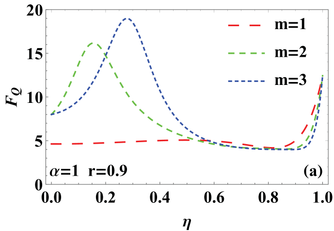
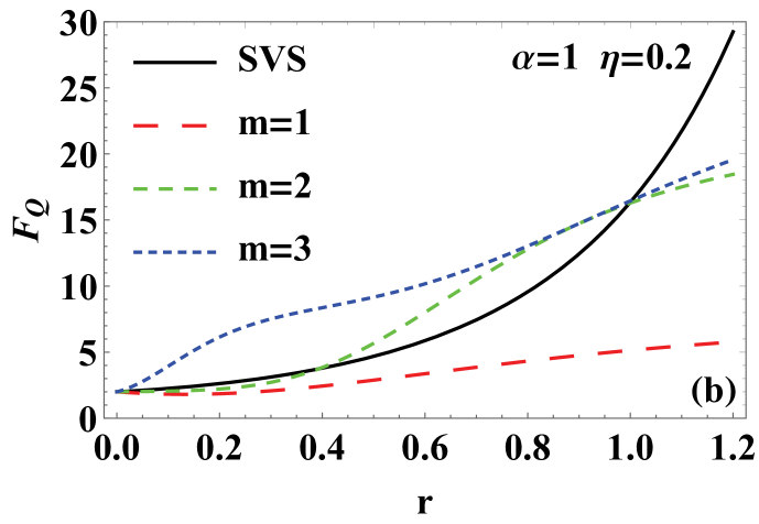
Figure 7: For the catalysis photon numbers $m=1,2,3$, (a) the variation of QFI with the transmissivity $\eta$ when fixed the coherent amplitude $\alpha=1$ and squeezing parameter $r=0.9$, (b) the variation of QFI with the squeezing parameter $r$ when fixed $\alpha=1$ and transmissivity $\eta=0.2$, and the black solid line corresponds to the SVS (without photon catalysis) is plotted for comparison.

Upon analysis of Fig. 7, it is evident that the QFI $F_{Q}$ varies with the relevant parameters of the transmissivity $\eta$ and squeezing parameter $r$ of PCSVS when the catalysis photon numbers $m=1,2,3$, and is then compared with the scenario of the CS and SVS as the input state. From Fig. 7(a), it is evident that for a fixed squeezing parameter $r=0.9$ and coherent amplitude $\alpha=1$, the QFI corresponding to the mixed CS and MC-SVS as inputs ($m=2,3$) at low transmissivity $\eta$ experiences a significant increase compared to the QFI without performing photon catalysis operation ($\eta=1$). This observation implies that at small $\eta$ values, multi-photon catalysis operation can effectively enhance the precision of phase measurement. Examining Fig. 7(b), it becomes evident that the QFI rises as both $r$ and $m$ increase for a constant transmissivity value of $\eta=0.2$ and coherent amplitude $\alpha=1$. Furthermore, it is noted that within a certain range of $r$, the QFI corresponding to the CS mixed with the MC-SVS as the input state surpasses that of the CS mixed with SVS.

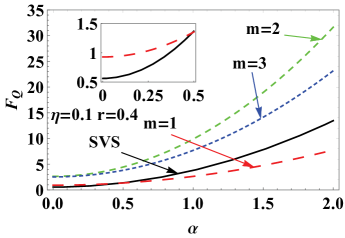
Figure 8: The QFI $F_{Q}$ as a function of the coherent amplitude $\alpha$ for the catalysis photon numbers $m=1,2,3$, transmissitivity $\eta=0.1$ and squeezing parameter $r=0.4$. The black solid line corresponds to the SVS (without photon catalysis) for comparison.

The plot in Fig. 8 illustrates the variation of the QFI $F_{Q}$ with the coherent amplitude $\alpha$, given a squeezing parameter of $r=0.4$ and transmissivity of $\eta=0.1$. It is evident from the figure that the QFI increases as $\alpha$ increases. Furthermore, we observe that the combination of the coherent state and the MC-SVS, with catalysis photon numbers $m=2,3$, presents a noticeable advantage in increasing the QFI compared to the CS mixed with SVS input MZI. Meanwhile, for the case of $m=1$, there is also a slight improvement when $\alpha$ is small.

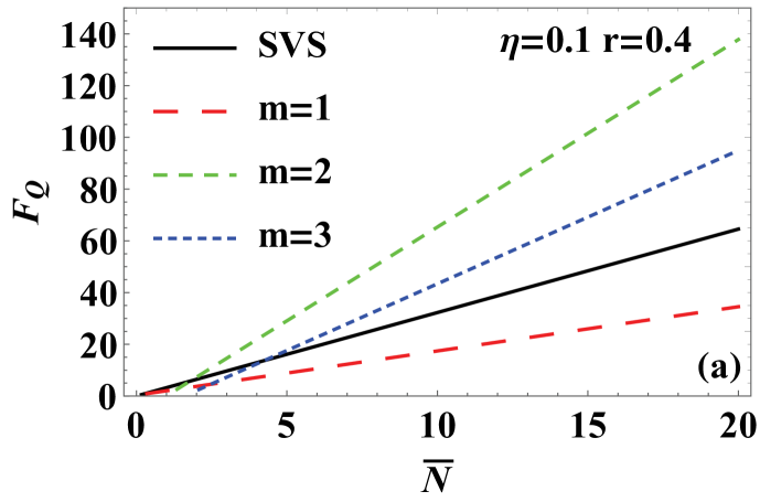
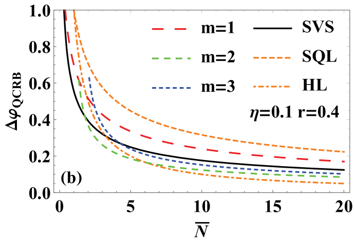
Figure 9: For the catalysis photon number $m=1,2,3$, transmissivity $\eta=0.1$ and squeezing parameter $r=0.4$, (a) the variation of QFI with the total average photon number $\bar{N}$, (b) the variation of QCRB with $\bar{N}$, the SQL, HL, and the case of SVS (without photon catalysis) are also plotted for comparison.

To analyze the connection between phase measurement precision and the energy of the input state, Fig. 9 illustrates the variations of QFI $F_{Q}$ and QCRB ($\Delta\varphi_{QCRB}=1/\sqrt{F_{Q}}$) concerning the total average photon number $\bar{N}$. In Fig. 9(a), the changes in QFI concerning $\bar{N}$ for different catalysis photon numbers $m=1,2,3$ are depicted, with a specific transmissivity $\eta=0.1$ and squeezing parameter $r=0.4$, and are compared with the scenario of the CS and SVS as inputs. It is evident that the QFI increases with $\bar{N}$, and the QFI for $m=2,3$ surpasses that of SVS (without photon catalysis) over a wide range of $\bar{N}$. Additionally, employing Eq. (22), the function plot of QCRB concerning $\bar{N}$ is presented in Fig. 9(b), compared with the SQL and HL. Fig. 9(b) clearly demonstrates that the QCRB gradually improves with increasing $\bar{N}$, effectively surpassing the SQL. Furthermore, the QCRB can approach or even exceed the HL when $\bar{N}$ is relatively small. Through further comparison, it is observed that multi-photon catalysis operation for $m=2,3$ can enhance the QCRB in comparison to the SVS case.

IV Effects of photon losses on phase sensitivity

In practical measurement processes, photon losses are inevitably present. Therefore, investigating the impact of photon losses on phase sensitivity is a vital issue. In this section, we examine the effects of photon losses before the parity detection (external losses, as depicted in Fig. 10(a)) and between the phase shifter and the second beam splitter (BS) BS2 (internal losses, as illustrated in Fig. 10(b)) on phase sensitivity.

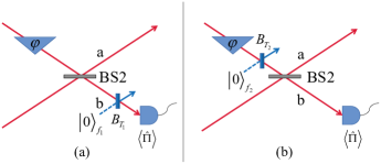
Figure 10: Theoretical model of parity detection under photon losses, including (a) external dissipation before parity detection, and (b) internal dissipation between the phase shifter and BS2.

IV.1 Equivalent parity detection under external losses

When considering the photon losses before parity detection (external losses), it is essential to define the parity operator under the photon losses in order to calculate the phase sensitivity with parity detection. As illustrated in Fig. 10(a), the external losses can be represented using a BS denoted as $B_{T_{1}}$. Its input-output relationship can be expressed as

$$B_{T_{1}}^{\dagger}\left(\begin{array}[]{c}b\\ f_{1}\end{array}\right)B_{T_{1}}=\left(\begin{array}[]{cc}\sqrt{T_{1}}&\sqrt{1-T_{1}}\\ -\sqrt{1-T_{1}}&\sqrt{T_{1}}\end{array}\right)\left(\begin{array}[]{c}b\\ f_{1}\end{array}\right),$$ (26)

where $b$ ($b^{\dagger}$) and $f_{1}$ ($f_{1}^{\dagger}$) are the photon annihilation (creation) operators corresponding to the mode $b$ in MZI and the dissipative mode $f_{1}$ respectively, and $T_{1}$ represents the transmissivity of the BS, ranging from $0$ to $1$. The larger the value of $T_{1}$, the smaller the photon losses. $T_{1}=1$ corresponds to the ideal situation without losses. To derive the phase sensitivity in the presence of external losses, it is necessary to initially express the parity operator in the ideal case as a Weyl ordering form [49], i.e.,

$$\Pi_{b}=\frac{\pi}{2}\begin{array}[]{c}\colon\\ \colon\end{array}\delta\left(b\right)\delta\left(b^{{\dagger}}\right)\begin{array}[]{c}\colon\\ \colon\end{array},\$$ (27)

where$\begin{array}[]{c}\colon\\ \colon\end{array}\bullet\begin{array}[]{c}\colon\\ \colon\end{array}$ is the Weyl ordering and $\delta\left(\cdot\right)$ represents the delta function. Combining Eqs. (26) and (27), using the Weyl invariance under similarity transformations [50, 51], and considering the vacuum noise $\left|0\right\rangle_{f_{1}}$ at the input of the dissipative mode $f_{1}$, the parity operator under external losses can be expressed as

$$\Pi_{b}^{loss} = \frac{\pi}{2}\text{Tr}\left[\left|0\right\rangle_{f_{1}}\left\langle 0\right|\begin{array}[]{c}\colon\\ \colon\end{array}B_{T_{1}}^{\dagger}\delta\left(b\right)\delta\left(b^{{\dagger}}\right)B_{T_{1}}\begin{array}[]{c}\colon\\ \colon\end{array}\right]$$ (32)

$$= \frac{\pi}{2}\text{Tr}\left[\left|0\right\rangle_{f_{1}}\left\langle 0\right|\begin{array}[]{c}\colon\\ \colon\end{array}\delta(\sqrt{T_{1}}b+\sqrt{1-T_{1}}f_{1})\right.$$ (38)

$$\left.\times\delta\left(\sqrt{T_{1}}b^{{\dagger}}+\sqrt{1-T_{1}}f_{1}^{{\dagger}}\right)\begin{array}[]{c}\colon\\ \colon\end{array}\right].$$

Utilizing the normal product form of the Wigner operator [52, 53] $\Delta_{\alpha}\left(\alpha\right)=\frac{1}{\pi}\colon\exp\left[-2\left(a-\alpha\right)\left(a^{\dagger}-\alpha^{\ast}\right)\right]\colon$and $\Delta_{\beta}\left(\beta\right)=\frac{1}{\pi}\colon\exp\left[-2\left(b-\beta\right)\left(b^{\dagger}-\beta^{\ast}\right)\right]\colon$, the classical correspondence of Weyl ordering operator can be expressed as follows [51]

$$\begin{array}[]{c}\colon\\ \colon\end{array}f\left(a,a^{{\dagger}},b,b^{{\dagger}}\right)\begin{array}[]{c}\colon\\ \colon\end{array}$$ (43)

$$= 4\int d^{2}\alpha d^{2}\beta f\left(\alpha,\alpha^{\ast},\beta,\beta^{\ast}\right)\Delta_{a}\left(\alpha\right)\Delta_{b}\left(\beta\right).\$$ (44)

According to Eq. (44), $\Pi_{b}^{loss}$ can be further derived based on Eq. (38) as follows

$$\Pi_{b}^{loss} = 2\pi\int\frac{d^{2}\beta d^{2}\gamma}{\pi^{2}}\delta(\sqrt{T_{1}}\beta+\sqrt{1-T_{1}}\gamma)$$ (45)

$$\times\delta(\sqrt{T_{1}}\beta^{\ast}+\sqrt{1-T_{1}}\gamma^{\ast})$$

$$\times Tr\left[\left|0\right\rangle_{f_{1}}\left\langle 0\right|\Delta_{\alpha}\left(\alpha\right)\Delta_{\beta}\left(\beta\right)\right]$$

$$= \colon\exp\left(-2T_{1}b^{\dagger}b\right)\colon=\left(1-2T_{1}\right)^{b^{\dagger}b}.\$$

Based on Eqs. (9) and (45), the average value of the parity operator under external losses for the output state of MZI can be derived as

$$\left\langle\Pi_{b}^{loss}\right\rangle=\hat{D}\frac{\varepsilon\exp\left[\frac{A_{1}T_{1}\left(\cos\varphi-1\right)+A_{2}}{A_{1}}\alpha^{2}\right]}{\sqrt{A_{1}}},\$$ (46)

where

$$A_{1} = 1-4W_{1}W\left[1-T_{1}\left(\cos\varphi+1\right)\right]^{2},$$

$$A_{2} = 2WT_{1}^{2}\sin^{2}\varphi$$ (47)

$$-4W_{1}WT_{1}^{2}\sin^{2}\varphi\left[T_{1}\left(\cos\varphi+1\right)-1\right].\$$

The phase sensitivity $\Delta\varphi$ in the case of external dissipation can be obtained using an error propagation formula similar to Eq. (22).

IV.2 Equivalent parity detection under internal losses

As depicted in Fig. 10(b), the process of photon losses (internal losses) between the phase shifter and BS2 can be simulated by the BS $B_{T_{2}}$, where the input states of $B_{T_{2}}$ correspond to the signal light of mode $b$ and vacuum noise $\left|0\right\rangle_{f_{2}}$ of dissipation mode $f_{2}$. The corresponding input-output relation is given by

$$B_{T_{2}}^{\dagger}\left(\begin{array}[]{c}b\\ f_{2}\end{array}\right)B_{T_{2}}=\left(\begin{array}[]{cc}\sqrt{T_{2}}&\sqrt{1-T_{2}}\\ -\sqrt{1-T_{2}}&\sqrt{T_{2}}\end{array}\right)\left(\begin{array}[]{c}b\\ f_{2}\end{array}\right),$$ (48)

where $b$ ($b^{\dagger}$) and $f_{2}$ ($f_{2}^{\dagger}$) are the photon annihilation (creation) operators corresponding to the mode $b$ and the dissipative mode $f_{2}$, respectively. $T_{2}$ represents the transmissivity of the beam splitter $B_{T_{2}}$, which ranges from $0$ to $1$. The larger the value of $T_{2}$, the smaller the photon losses. $T_{2}=1$ corresponds to the ideal situation of no losses. Therefore, in the Heisenberg picture, for the case of internal dissipation, by using the transformation relation of the equivalent operator of MZI considering internal dissipation, the operator representing parity detection of the input state after passing through the entire lossy interferometer can be given by

$$\widetilde{\Pi}_{b}^{loss}=\left.{}_{f_{2}}\left\langle 0\right|B_{1}^{\dagger}U^{\dagger}\left(\varphi\right)B_{T_{2}}^{\dagger}B_{2}^{\dagger}\Pi_{b}B_{2}B_{T_{2}}U\left(\varphi\right)B_{1}\left|0\right\rangle_{f_{2}}\right..$$ (49)

Applying the method similar to that used to obtain the parity operator in the case of external dissipation, and combining Eq. (49) with the transformation relationship of the two $50:50$ BSs in the MZI

$$B_{1}^{\dagger}\binom{a}{b}B_{1} = \frac{\sqrt{2}}{2}\left(\begin{array}[]{cc}1&-i\\ -i&1\end{array}\right)\binom{a}{b},$$ (52)

$$B_{2}^{\dagger}\binom{a}{b}B_{2} = \frac{\sqrt{2}}{2}\left(\begin{array}[]{cc}1&i\\ i&1\end{array}\right)\binom{a}{b},$$ (55)

the expression for the normal-ordered parity operator in the case of internal dissipation can be obtained as follows

$$\widetilde{\Pi}_{b}^{loss}=\colon e^{X_{1}a^{\dagger}a-X_{2}b^{\dagger}a-X_{2}^{\ast}a^{\dagger}b+X_{3}b^{\dagger}b}\colon,$$ (56)

where

$$X_{1} = \frac{2\sqrt{T_{2}}\cos\varphi-1-T_{2}}{2},$$

$$X_{2} = \frac{\left(T_{2}+1\right)^{2}-4T_{2}\cos^{2}\varphi}{2\left(iT_{2}-i+2\sqrt{T_{2}}\sin\varphi\right)},$$

$$X_{3} = -\frac{2\sqrt{T_{2}}\cos\varphi+1+T_{2}}{2}.$$ (57)

Upon combining with the expression of the input states, the average value of the corresponding parity operator in the case of internal dissipation can be further obtained as follows

$$\left\langle\widetilde{\Pi}_{b}^{loss}\right\rangle=\left\langle in\right|\widetilde{\Pi}_{b}^{loss}\left|in\right\rangle=\hat{D}\frac{\varepsilon\exp\left[\frac{B_{1}X_{1}+B_{2}}{B_{1}}\alpha^{2}\right]}{\sqrt{B_{1}}},$$ (58)

where

$$B_{1} = 1-4W_{1}W\left(1+X_{3}\right)^{2},$$

$$B_{2} = W_{1}X_{2}^{2}+WX_{2}^{\ast 2}+4W_{1}W\left|X_{2}\right|^{2}\left(1+X_{3}\right).$$ (59)

Further substituting of Eq. (58) into the error propagation formula, we can obtain the phase sensitivity $\Delta\varphi_{L}$ with parity detection in the case of internal dissipation.

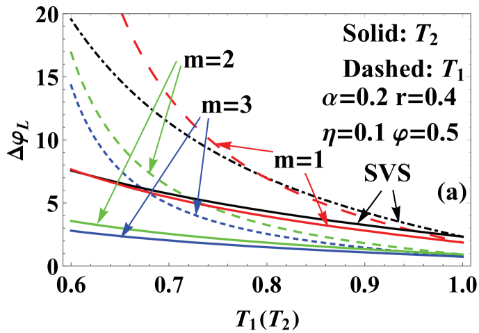
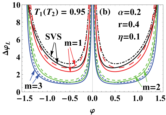
Figure 11: For the catalysis photon numbers $m=1,2,3$, and fixed the transmissivity $\eta=0.1$, the squeezing parameter $r=0.4$, and the coherent amplitude $\alpha=0.2$, (a) the phase sensitivity $\Delta\varphi_{L}$ under photon losses as a function of the transmissivity of $B_{T_{1}}$($B_{T_{2}}$) $T_{1}$($T_{2}$) for the phase shift $\varphi=0.5$, (b) $\Delta\varphi_{L}$ as a function of $\varphi$ for $T_{1}=T_{2}=0.95$. The dashed (solid) lines correspond to the cases of external (internal) dissipation, and the black lines correspond to the SVS (without photon catalysis) for comparison.

IV.3 The effects of external and internal losses

In order to clearly analyze the impact of photon losses on phase sensitivity, an image of the phase sensitivity $\Delta\varphi_{L}$ under photon losses is presented as a function of the transmissivity $T_{1}$($T_{2}$) of the optical BS $B_{T_{1}}$($B_{T_{2}}$) in Fig. 11(a) for the different catalysis photon numbers $m=1,2,3$, phase shift $\varphi=0.5$, and fixed the other relevant parameters ($\eta,r,\alpha$) of the input state, and comparing it with the SVS (without photon catalysis). It is evident that $\Delta\varphi_{L}$ increases as $T_{1}$($T_{2}$) decreases, indicating that photon losses worsen the phase sensitivity. Fig. 11(b) demonstrates the variation of $\Delta\varphi_{L}$ with $\varphi$ for $m=1,2$, and $3$, and $\eta=0.1$, when $r=0.4$, $\alpha=0.2$, and $T_{1}=T_{2}=0.95$. These results are compared with those of the CS mixed with SVS as inputs. Fig. 11 suggests that, under photon losses, the optimal value of $\Delta\varphi_{L}$ is achieved when $\varphi$ deviates from $0$; conversely, the value of $\Delta\varphi_{L}$ becomes extremely large when $\varphi$ approaches $0$. Additionally, it is evident from Fig. 11 that the phase sensitivity of the external dissipation, corresponding to the dashed line, is inferior to that of the internal dissipation, corresponding to the solid line, indicating a greater impact of external dissipation on phase sensitivity. Despite photon losses in the actual measurement process, especially for the MC-SVS with $m=2,3$, $\Delta\varphi_{L}$ can still be efficiently improved compared to the CS mixed with SVS when using a mix of CS and the PCSVS as inputs. Furthermore, for external dissipation, a smaller loss (corresponding to a larger $T_{1}$) is required to achieve better phase sensitivity at $m=1$ than the SVS case (see Fig. 11(a)).

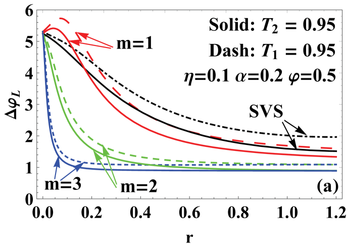
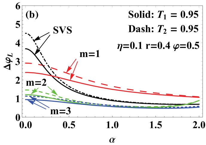
Figure 12: For the catalysis photon numbers $m=1,2,3$, and fixed phase shift $\varphi=0.5$, with transmissivity values $T_{1}=T_{2}=0.95$ and $\eta=0.1$, (a) the phase sensitivity $\Delta\varphi_{L}$ under photon losses as a function of the squeezing parameter $r$ with the coherent amplitude $\alpha=0.2$, and (b) $\Delta\varphi_{L}$ as a function of $\alpha$ when $r=0.9$. The dashed (solid) lines represent external (internal) dissipation, and the black lines represent the SVS (without photon catalysis) for comparison.

From Fig. 12, the variation of the phase sensitivity $\Delta\varphi_{L}$ under photon losses with respect to the squeezing parameter $r$ and the coherent amplitude $\alpha$ is visually observed under the conditions of $\varphi=0.5$, transmissivity $T_{1}=T_{2}=0.95$, and $\eta=0.1$. As depicted in Fig. 12(a), it is evident that for $\alpha=0.2$, $\Delta\varphi_{L}$ significantly improves with the increase of $r$ within a specific range. Similarly, as indicated in Fig. 12(b), for the given condition of $r=0.4$, $\Delta\varphi_{L}$ can improve with the increase of $\alpha$ within a certain range. It is apparent from Fig. 12 that external dissipation has a more pronounced effect on phase sensitivity. Furthermore, in the presence of photon losses, the CS, when mixed with the PCSVS, can notably enhance the phase sensitivity, particularly for the MC-SVS ($m=2,3$), relative to the SVS (without photon catalysis).

V
The impact of photon losses on QFI

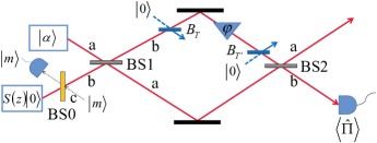
Figure 13: Schematic diagram of lossy MZI with CS mixed PCSVS as input.

In the field of quantum metrology, the Cramér-Rao bound theory of QFI sets the limit for phase estimation. However, this limitation can be influenced by environmental factors. This section focuses primarily on the impact of photon losses in MZI on QFI. As depicted in Fig. 13, it is assumed that photon losses occur in the optical path of mode $b$, primarily located before and after the phase shifter, simulated by the optical BSs $B_{T}$ and $B_{T^{{}^{\prime}}}$. According to Ref. [54] in this scenario, the QFI can be computed as

$$F_{QL}\leq C_{Q}=4\left[\left\langle\psi\right|\hat{H}_{1}\left|\psi\right\rangle-\left|\left\langle\psi\right|\hat{H}_{2}\left|\psi\right\rangle\right|^{2}\right],$$ (60)

where, $\left|\psi\right\rangle=e^{-i\frac{\pi}{2}J_{1}}\left|in\right\rangle$ is the quantum state that is input as a pure state and passing through BS1. By utilizing Kraus operators representation, we can express $H_{1,2}$ in the above equation as follows

$$\hat{H}_{1} = \sum\limits_{l}\frac{d\hat{\Pi}_{l}^{\dagger}\left(\varphi\right)}{d\varphi}\frac{d\hat{\Pi}_{l}\left(\varphi\right)}{d\varphi},$$

$$\hat{H}_{2} = i\sum\limits_{l}\frac{d\hat{\Pi}_{l}^{\dagger}\left(\varphi\right)}{d\varphi}\hat{\Pi}_{l}\left(\varphi\right),$$ (61)

where $\Pi_{l}\left(\varphi\right)$ is the Kraus operator

$$\hat{\Pi}_{l}\left(\varphi\right)=\sqrt{\frac{\left(1-T\right)^{l}}{l!}}e^{i\varphi\left(b^{\dagger}b-\gamma l\right)}T^{\frac{b^{\dagger}b}{2}}b^{l}.$$ (62)

In the equation, the transmissivity $T$ of optical BSs $B_{T}$ and $B_{T^{{}^{\prime}}}$ can be used to quantify the photon losses that occur on mode $b$ in MZI. Here, $T=0$ and $T=1$ respectively represent complete absorption and lossless scenarios. Parameter $\gamma=0$ and $\gamma=-1$ correspond to photon losses occurring before and after the phase shifter. By optimizing $\gamma$, the minimum value of $C_{Q}$ can be achieved. Thus, the QFI under the condition of photon losses can be obtained as

$$F_{QL}=\frac{4F_{Q}T\left\langle\psi\right|b^{\dagger}b\left|\psi\right\rangle}{\left(1-T\right)F_{Q}+4T\left\langle\psi\right|b^{\dagger}b\left|\psi\right\rangle}.$$ (63)

By using unitary transformations, one can derive

$$\left\langle\psi\right|b^{\dagger}b\left|\psi\right\rangle=\frac{1}{2}\left(\alpha^{2}+\hat{D}\frac{\varepsilon}{\left(1-4W_{1}W\right)^{\frac{3}{2}}}-1\right)=\frac{1}{2}\bar{N}.$$ (64)

By substituting Eqs. (24) and (64) into Eq. (63), one can obtain $F_{QL}$.

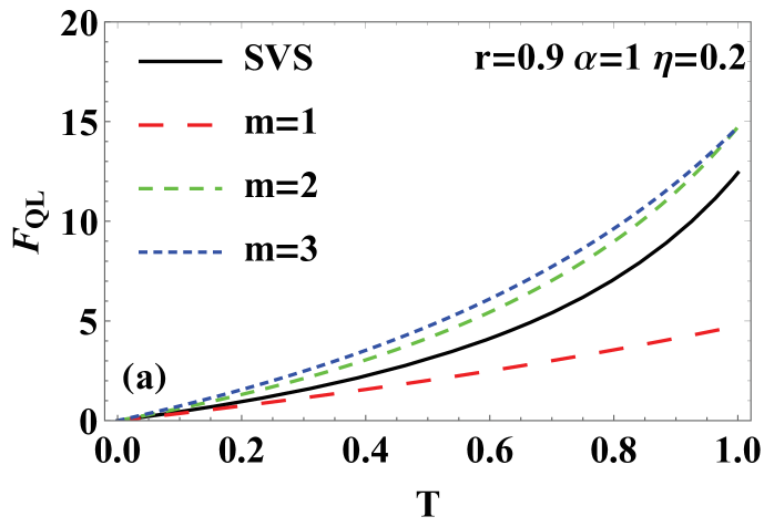
Figure 14: For the catalysis photon numbers $m=1,2,3$, fixed the squeezing parameter $r=0.9$, and coherent amplitude $\alpha=1$, (a) the variation of $F_{QL}$ as a function of the transmissivity $T$ when $\eta=0.2$, (b) $F_{QL}$ as a function of $\eta$ when $T=0.9$. The black solid line corresponds to the SVS (without photon catalysis) for comparison.

In order to analyze the impact of photon losses on QFI, we can obtain the variation of $F_{QL}$ with respect to its corresponding parameters based on its analytical expression. Fig. 14(a) displays the variation of $F_{QL}$ with the transmissivity $T$ of $B_{T}$ ($B_{T^{{}^{\prime}}}$), which simulates photon losses, for a given squeezing parameter $r=0.9$, coherent amplitude $\alpha=1$, and transmissivity $\eta=0.2$. Intuitively, it is observed that $F_{QL}$ increases with $T$, indicating that the QFI rises as photon losses decrease. Additionally, the QFI for the CS mixed with the MC-SVS ($m=2,3$), can increase relative to the case of CS mixed with the SVS as inputs. Furthermore, from Fig. 14(b), it is evident that the change in $F_{QL}$ with $\eta$, for $T=0.9$ with photon losses, when $\alpha=1$ and $r=0.9$, the case of $m=2,3$ can significantly increase compared to the SVS (without photon catalysis) case when $\eta$ is small.

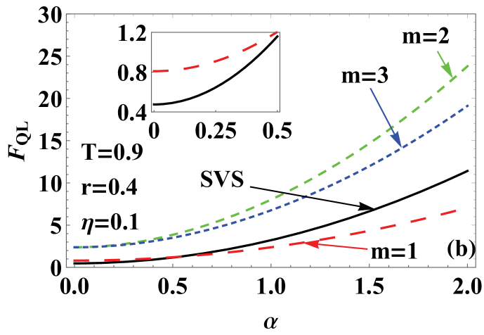
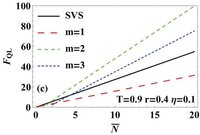
Figure 15: For the catalysis photon numbers $m=1,2,3$, and fixed the transmissivity $T=0.9$, (a) $F_{QL}$ as a function of the squeezing parameter $r$ when the coherent amplitude $\alpha=1$ and $\eta=0.2$, (b) $F_{QL}$ as a function of $\alpha$ when $r=0.4$ and $\eta=0.1$, and (c) $F_{QL}$ as a function of average photon number $\bar{N}$ when $r=0.4$ and $\eta=0.1$. The black solid line corresponds to the SVS (without photon catalysis) for comparison.

Fig. 15 illustrates the intuitive analysis of the relationship between $F_{QL}$ and the relevant parameters of the input resources in the presence of photon losses ($T=0.9$) with a fixed small transmissivity $\eta$. The clear variation pattern in Fig. 15 indicates that, even with photon losses, the QFI can increase by raising the squeezing parameter $r$, coherent amplitude $\alpha$, and average photon number $\bar{N}$. Additionally, it demonstrates that the CS mixed with MC-SVS with $m=2,3$ as input states can effectively increase the $F_{QL}$ compared to the input CS mixed with SVS. Particularly, from Fig. 15(b), it is evident that for the case of $m=1$ and a relatively small $r=0.4$, $F_{QL}$ can also be increased relative to SVS (without photon catalysis) in the range of small $\alpha$, which is relatively easy to achieve experimentally.

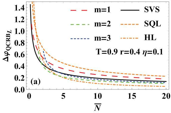
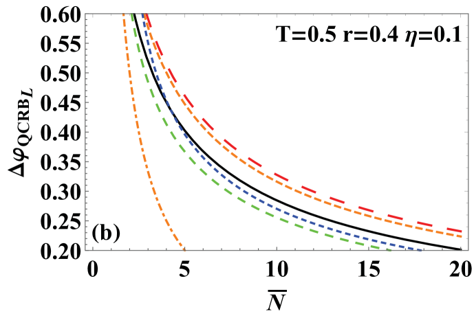
Figure 16: For the catalysis photon numbers $m=1,2,3$, and fixed the squeezing parameter $r=0.4$, and transmissivity $\eta=0.1$, (a) with transmissivity $T=0.9$, (b) with $T=0.5$, the variation of QCRB $\Delta\varphi_{QCRB_{L}}$ with respect to the average photon number $\overline{N}$. The black solid line, orange dashed line, and orange dotdashed line is respectively represent the SVS (without photon catalysis), SQL, and HL for comparison.

The variation of the QCRB ($\Delta\varphi_{QCRB_{L}}=1/\sqrt{F_{QL}}$) with the energy of the input CS mixed with PCSVS (corresponding to the average photon number $\bar{N}$) under the condition of photon losses, and its comparison with the case where CS mixed with SVS is used as the input state, are depicted in Fig. 16. The SQL and the HL are also included for comparison. The figure illustrates an improvement in QCRB with the increase of $\bar{N}$, and it exhibits a certain enhancement relative to CS mixed with SVS when the CS mixed with MC-SVS ($m=2,3$) as inputs. Furthermore, Fig. 16(a) clearly demonstrates that despite the existence of photon losses corresponding to transmissivity $T=0.9$, the QCRB can effectively surpass the SQL. Moreover, for small $\bar{N}$ values, the QCRB can approach or even exceed the HL. Additionally, as depicted in Fig. 16(b), it is observed that the case of $m=2,3$ can successfully exceed the SQL, even for relatively high photon losses corresponding to $T=0.5$. This observation indicates the strong robustness of the QCRB for the scheme involving the CS mixed with MC-SVS as inputs against photon losses.

VI
Conclusion

In this study, we focused on investigating the precision of phase measurement in MZI using a CS mixed with PCSVS as input state, employing both the phase sensitivity of parity detection and the QFI. The findings indicate that the incorporation of photon catalysis, particularly through multi-photon catalysis operations, leads to a substantial enhancement in phase measurement precision compared to using CS mixed with SVS as input. In an ideal scenario involving the input of MZI with CS mixed with PCSVS, and with the implementation of parity detection at the output port, the adjustment of the transmissivity $\eta$ of the BS preparing the PCSVS can effectively enhance the resolution of the phase shift $\varphi$. Consequently, the optimization of $\eta$ is crucial for improving phase sensitivity. It was observed that the optimal point for $\Delta\varphi$ occurs at $\varphi=0$, and for relatively small $\eta$, the phase sensitivity $\Delta\varphi$ and QFI are significantly improved in the scheme of employing CS mixed with MC-SVS (the catalysis photon numbers $m=2,3$) as input in MZI, as compared to CS mixed with SVS as the input state. Furthermore, when the squeezing parameter $r$ and coherent amplitude $\alpha$ are small, the phase sensitivity $\Delta\varphi$ and QFI of $m=1$ is also enhanced relative to that of the SVS (without photon catalysis). Moreover, by increasing $r$, $\alpha$ and the total average number of photons $\overline{N}$ corresponding to the energy of the input resource, the QFI and $\Delta\varphi$ can be improved. Notably, in the case of $m=2,3$, the phase sensitivity $\Delta\varphi$ and the QCRB can surpass the SQL and even exceed the HL when compared with CS mixed with SVS as the input state.

Our study delved further into analyzing the phase sensitivity and QFI in the presence of photon losses in practical scenarios. The findings revealed that external dissipation has a more pronounced impact on phase sensitivity than internal dissipation. Although photon losses will reduce phase sensitivity and QFI, it is still possible to increase $r$, $\alpha$, and $\overline{N}$ at low $\eta$ to make multi-photon catalysis operation more effectively improve phase sensitivity and QFI. Additionally, the mixing of CS and MC-SVS can significantly improve phase sensitivity and the QFI better than the case of CS mixed with SVS as the input state, while there is also a certain improvement for $m=1$ when $r$ and $\alpha$ are relatively small. Moreover, in the presence of photon losses, the QCRB can still significantly outperform the SQL.

Overall, employing the scheme of mixing CS with PCSVS, especially when mixed with MC-SVS as input in MZI, significantly enhances phase measurement accuracy. Our findings hold significant importance in advancing quantum measurement for practical applications.

- [1] H. Vahlbruch, D. Wilken, M. Mehmet, and B. Willke, Laser Power Stabilization beyond the Shot Noise Limit Using Squeezed Light, Phys. Rev. Lett. 121, 173601 (2018).
- [2] E. Oelker, L. Barsotti, S. Dwyer, D. Sigg, and N. Mavalvala, Squeezed light for advanced gravitational wave detectors and beyond, Opt. Express 22, 021106 (2014).
- [3] X. Q. Xiao, E. S. Matekole, J. K. Zhao, G. H. Zeng, J. P. Dowling, and H. Lee, Enhanced phase estimation with coherently boosted two-mode squeezed beams and its application to optical gyroscopes Phys. Rev. A 102, 022614 (2020).
- [4] A. Kolkiran and G. S. Agarwal, Heisenberg limited Sagnac interferometry, Opt. Express 15, 6798 (2007).
- [5] J. Xin, J. Liu, and J. Jing, Nonlinear Sagnac interferometer based on the four-wave mixing process, Opt. Express 25, 1350-1359 (2017).
- [6] C. Lee, J. Huang, H. Deng, H. Dai, and J. Xu, Nonlinear quantum interferometry with Bose condensed atoms, Front. Phys. 7, 109-130 (2012).
- [7] A. C. J. Wade, J. F. Sherson, and K. Molmer, Squeezing and Entanglement of Density Oscillations in a Bose-Einstein Condensate, Phys. Rev. Lett. 115, 060401 (2015).
- [8] R. Nair and M. Tsang, Far-Field Superresolution of Thermal Electromagnetic Sources at the Quantum Limit, Phys. Rev. Lett. 117, 190801 (2016).
- [9] M. Tsang, Quantum limits to optical point-source localization, Optica 2, 646-653 (2015).
- [10] J. Zhang and M. Sarovar, Quantum Hamiltonian Identification from Measurement Time Traces, Phys. Rev. Lett. 113, 080401 (2014).
- [11] F. Jia, W. Ye, Q. Wang, L. Y. Hu, and H. Y. Fan, Comparison of nonclassical properties resulting from non-Gaussian operations, Laser Phys. Lett. 16, 015201 (2019).
- [12] M. O. Scully and M. S. Zubairy, Quantum Optics (Cambridge University Press, Cambridge, 1997).
- [13] P. Luca and S. Augusto, Mach-Zehender Interferometry at the Heisenberg Limit with Coherent and Squeezed-Vaccum Light, Phys. Rev. Lett. 100, 073601 (2008).
- [14] X. Yu, X. Zhao, L. Y. Shen, Y. Y. Shao, J. Liu, and X. G. Wang, Maximal quantum Fisher information for phase estimation without initial parity, Opt. Express 26, 16292 (2018).
- [15] C. M. Caves, Quantum-mechanical noise in an interferometer, Phys. Rev. D 23, 1693 (1981).
- [16] V. Giovannetti, S. Lloyd, and L. Maccone, Advances in quantum metrology, Nat. Photon, 5, 222 (2011).
- [17] C. W. Helstrom, Quantum detection and estimation theory (Academic, New York, 1976).
- [18] A. N. Boto, P. Kok, D. S. Abrams, S. L. Braunstein, C. P. Williams, and J. P. Dowling, Quantum interferometric optical lithography: exploiting entanglement to beat the diffraction limit, Phys. Rev. Lett. 85, 2733 (2000).
- [19] R. A. Campos, Christopher C. Gerry, and A. Benmoussa, Optical interferometry at the Heisenberg limit with twin Fock states and parity measurements, Phys. Rev. A 68, 023810 (2003).
- [20] H. Lee, P. Kok, and J. P. Dowling, A quantum Rosetta stone for interferometry, J. Mod. Opt. 49, 2325 (2002).
- [21] T. Nagata, R. Okamoto, J. L. Obrien, K. Sasaki, and S. Takeuchi, Beating the Standard Quantum Limit with Four-Entangled Photons, Science, 316, 726 (2007).
- [22] J. P. Dowling, Quantum optical metrology – the lowdown on high-N00N states, Contemp. Phys. 49, 125 (2008).
- [23] G. Y. Xiang, B. L. Higgins, D. W. Berry, H. M. Wiseman, and G. J. Pryde, Entanglement-enhanced measurement of a competely unknown optical phase, Nat. Photon. 5, 43 (2011).
- [24] H. Cable and G. A. Durkin, Parameter Estimation with Entangled Photons Produced by Parametric Down-Conversion, Phys. Rev. Lett. 105, 013603 (2010).
- [25] R. A. Campos, Christopher C. Gerry, and A. Benmoussa, Optical interferometry at the Heisenberg limit with twin Fock states and parity measurements, Phys. Rev. A 68, 023810 (2003).
- [26] P. M. Anisimov, G. M. Raterman, A. Chiruvelli, W. N. Plick, S. D. Huver, H. Lee, and J. P. Dowling, Quantum Metrology with Two-Mode Squeezed Vacuum: Parity Detection Beats the Heisenberg Limit, Phys. Rev. Lett. 104, 103602 (2010).
- [27] R. Birrittella, J. Mimih, and C. C. Gerry, Multiphoton quantum interference at a beam splitter and the approach to Heisenberg-limited interferometry, Phys. Rev. A 86, 063828 (2012).
- [28] S. K. Chang, C. P. Wei, H. Zhang, Y. Xia, W. Ye, and L. Y. Hu, Enhanced phase sensitivity with a nonconventional interferometer and nonlinear phase shifter, Phys. Lett. A 384, 126755 (2020).
- [29] S. K. Chang, W. Ye, H. Zhang, L. Y. Hu, J. H. Huang, and S. Q. Liu, Improvement of phase sensitivity in an SU(1,1) interferometer via a phase shift induced by a Kerr medium, Phys. Rev. A 105, 033704 (2022).
- [30] Q. K. Gong, X. L. Hu, D. Li, C. H. Yuan, Z. Y. Ou, and W. P. Zhang, Intramode-correlation-enhanced phase sensitivities in an SU(1,1) interferometer, Phys. Rev. A 96, 033809 (2017).
- [31] Z. K. Zhao, H. Zhang, Y. B. Huang, and L. Y. Hu, Phase estimation of a Mach-Zehnder interferometer via the Laguerre excitation squeezed state, Opt. Express 31, 17645 (2023).
- [32] J. Liu, T. Shao, Y. X. Wang, M. M. Zhang, Y. Y. Hu, D. X. Chen, and D. Wei, Enhancement of the phase sensitivity with two-mode squeezed coherent state based on a Mach-Zehnder interferometer, Opt. Express 31, 27735 (2023).
- [33] K. P. Seshadreesan, P. M. Anisimov, H. Lee, J. P. Dowling, Parity detection achieves the Heisenberg limit in interferomery with coherent mixed with squeezed vacuum light, New J. Phys. 13, 083026 (2011).
- [34] L. L. Guo, Y. F. Yu, and Z. M. Zhang, Improving the phase sensitivity of an SU(1,1) interferometer with photon-added squeezed vacuum light, Opt. Express. 26, 029099 (2018).
- [35] R. Carranza and C. C. Gerry, Photon-subtracted two-mode squeezed vacuum states and applications to quantum optical interferometry, J. Opt. Soc. Am. B 29, 2581 (2012).
- [36] Y. Ouyang, S. Wang, and L. J. Zhang, Quantum optical interferometry via the photon-added two-mode squeezed vacuum states, J. Opt. Soc. Am. B 33, 1373 (2016).
- [37] D. Braun, P. Jian, O. Pinel, and N. Treps, Precision measurements with photon-subtracted or photon-added Gaussian states, Phys. Rev. A 90, 013821 (2014).
- [38] R. Birrittella and C. C. Gerry, Quantum optical interferometry via the mixing of coherent and photon-subtracted squeezed vacuum states of light, J. Opt. Soc. Am. B 31, 586 (2014).
- [39] S. Wang, X. X. Xu, Y. J. Xu, and L. J. Zhang, Quantum interferometry via a coherent state mixed with a photon-added squeezed vacuum state, Opt. Commun. 444, 102 (2019).
- [40] H. Zhang, W. Ye, C. P. Wei, Y. Xia, S. K. Chang, Z. Y. Liao, and L. Y. Hu, Improved phase sensitivity in quantum optical interferometer based on muti-photon catalytic two-mode squeezed vacuum states, Phys. Rev. A 103, 013705 (2021).
- [41] Y. K. Xu, S. K. Chang, C. J. Liu, L. Y. Hu, and S. Q. Liu, Phase estimation of an SU(1,1) interferometer with a coherent superposition squeezed vacuum in a realistic case, Opt. Express 30, 38178 (2022).
- [42] Y. K. Xu, T. Zhao, Q. Q. Kang, C. J. Liu, L. Y. Hu, and S. Q. Liu, Phase sensitivty of an SU(1,1) interferometer in photon-loss via photon operations, Opt. Express 31, 8414 (2023).
- [43] J. Xin, Phase sensitivity enhancement for the SU(1,1) interferometer using photon level operations, Opt. Express 29, 43970 (2021).
- [44] K. Zhang, Y. H. Lv, Y. Guo, J. T. Jing, and W. M. Liu, Enhancing the precision of a phase measurement through phase-sensitive non-Gaussianity, Phys. Rev. A 105, 042607 (2022).
- [45] F. Jia, W. Ye, Q. Wang, L. Y. Hu, and H. Y. Fan, Comparison of nonclassical properties resulting from non-Gaussian operations, Laser Phys. Lett. 16, 015201 (2019).
- [46] B. Yurke, S. L. McCall, and J. R. Klauder, SU(2) and SU(1,1) interferometers, Phys. Rev. A 33, 4033 (1986).
- [47] R. R. Puri, Mathematical methods of quantum optics (Springer-Verlag, Berlin, 2001), Appendix A.
- [48] J. Liu, X. Jing, W. Zhong, and X. Wang, Quantum Fisher Information for density matrices with arbitrary ranks, Commun. Theor. Phys. 61, 45-50 (2014).
- [49] L. Y. Hu and H. Y. Fan, Entangled state for constructing a generalized phase-space representation and its statistical behavior, Phys. Rev. A 80, 022115 (2009).
- [50] H. Y. Fan, Newton–Leibniz integration for ket-bra oper ators in quantum mechanics (V)—Deriving normally or dered bivariate-normal-distribution form of density oper ators and developing their phase space formalism, Ann. Phys. (NY) 323, 1502 (2008).
- [51] H. Weyl, Quantenmechanik und Gruppentheorie, Z. Phys. 46, 1 (1927).
- [52] E. P. Wigner, On the Quantum Correction for Thermudynamic Equilibrium, Phys. Rev. 40, 749 (1932).
- [53] H. Y. Fan and H. R. Zaidi, Application of IWOP technique to the generalized Weyl correspondence, Phys. Lett. A 124, 303 (1987).
- [54] B. M. Escher, R. L. de Matos Filho, and L. Davidovich, General framework for estimating the ultimate precision limit in noisy quantum-enhanced metrology, Nat. Phys. 7, 406 (2011).