An Entangled Universe

Abstract

We propose a possible quantum signature of the early Universe that could lead to observational imprints of the quantum nature of the inflationary period. Graviton production in the presence of an inflaton scalar field results in entangled states in polarization. This is because of a non-trivial effect due to the derivatives on two scalar fluctuations and it provides a fingerprint that depends on the polarization of the graviton that Alice and/or Bob measured in their patch. At horizon crossing, interactions between the gravitons and inflatons perform the required Bell experiments leading to a definitive measure. We hint how this signature could be measured in the high-order correlation function of galaxies, in particular on the halo bias and the intrinsic alignment.

1 Introduction

Inflation is a period of quasi-exponential expansion of the early Universe, i.e. a de Sitter stage with slightly broken time-translational symmetry to allow for a graceful exit [1, 2, 3, 4, 5]:

$$a(t)\sim a_{i}\,e^{H_{\Lambda}t}\,\,,$$ (1.1)

where $a$ is the scale factor, with initial value $a_{i}$ and $H_{\Lambda}=(8\pi G\varepsilon_{\Lambda}/3)^{1/2}$, where $\varepsilon_{\Lambda}$ is the constant energy density of a perfect fluid with positive cosmological constant $\Lambda$, with equation of state $p_{\Lambda}=-\varepsilon_{\Lambda}$.

The presence of an inflationary stage previous to the Big Bang (or what used to be called “Big Bang” before the upcoming theory of inflation) solves in a natural manner the fine tuning and naturalness problems of the previous theory (horizon problem, flatness problem/fine tuning of the initial conditions, and others - for reference, see for example [5]) while keeping its successful predictions like Big Bang Nucleosynthesis. It also introduces a natural way to explain the inhomogeneities and anisotropies in the Universe that gave rise to the formation of the cosmological structures we observe today. Quantum fluctuations in the fields present during inflation (in its most minimal form, just the spacetime-metric field, and a scalar field called the inflaton) get stretched by the exponential expansion to cosmological distances. Their “size” (physical wavelength) grows proportional to $a$, while their amplitude decays as $a^{-1}$. The curvature scale $H_{\Lambda}^{-1}$ (or Hubble horizon) remains almost constant during inflation. Thus, for any mode of fixed comoving wavenumber $k$, the physical wavelength $\lambda_{ph}=2\pi(a/k)$ of a quantum fluctuation generated inside the Hubble horizon will soon become larger than $H_{\Lambda}^{-1}$. Therefore, the corresponding mode leaves the horizon, and starts “feeling” the curvature of spacetime. At horizon crossing, its amplitude freezes and remains almost constant until the end of the inflationary stage. Once inflation is over, the radiation dominated era starts (decelerating Hubble expansion), during which the curvature scale $H_{\text{rad}}^{-1}$ starts growing at a rate $a/\dot{a}$. At this point, the now large fluctuations reenter the Hubble horizon as density perturbations of cosmological scale, and as gravitational waves. These density perturbations work as classical gravitational seeds for the formation of large-scale structures. Those modes that left the horizon the latest (in the last $8$ e-folds of inflation approximately, see [6], sec. 8.4) will be the first ones to reenter, and are the ones relevant in determining the structures in our observable scales.

In this context, there is a somewhat natural question that emerges: at what point does a quantum fluctuation generated during inflation stop being of quantum nature? The analysis that we apply to the Cosmic Microwave Background (CMB), which provides us with the earliest observational features of the Universe so far, and to large scale structure survey’s data, is classical. But where did the quantum nature of the gravitational seeds go? It is still an open question how this classicalization of quantum fluctuations occurs. If any signal of the early nature of the quantum fluctuation remains, this should be imprinted in some current observable, maybe in the form of non-gaussianities in the CMB anisotropies, or in higher-order correlation functions of galaxy distributions, or some other observable.

There has been previous work in the literature trying to search for quantum signals of the early Universe[7, 8, 9, 10, 11, 12, 13, 14, 15, 16, 17, 18, 19, 20, 21, 22, 23, 24, 25, 26, 27, 28]. Quantum discord (a measure of “quantumness”) of inflationary perturbations is calculated in [29] and suggests some features to probe different levels of discordance in CMB descriptions. Possible observational signatures in the CMB of graviton exchange between tensor and scalar fluctuations are discussed in [30]. On the other hand, due to the environment, the potential decoherence of quantumness upon classicalization has been widely discussed in literature, e.g., see [31, 32, 33, 34, 35, 36, 37, 20, 38, 27, 39, 40]. For example, in [41], they discuss how the CMB polarization components $\bf E$ and $\bf B$ are modified due to entanglement of scalar and tensor fluctuations. Regarding primordial gravitons, a possible source of decoherence should also include the nonlinear interaction between tensor modes [42] and the scalar-tensor interaction [27, 39, 40]. Another possibility is to add extra fields to the simplest model of inflation such that one can construct Bell inequalities as done in [43].

In this work, we suggest a mechanism by which entangled states are created during inflation, via the interaction of gravitons and inflatons. We describe plausible processes by which the quantum nature of the tensor fluctuations of the metric field (i.e. gravitons) during inflation is made explicit. We discuss how, through interaction with their environment, gravitons may imprint this quantumness into some observable quantity. We then propose what this observable quantity might be.

2 Perturbations during inflation

Let us briefly review the basics of quantum fluctuations generated during inflation. While this is textbook material, it is useful as to briefly setup the notation and make the article self-consistent for readers not specialized in the early Universe. More specialized readers can proceed directly to section 2.3.

Any quantum field fluctuates due to the need to satisfy the equations of motion and the Heisenberg uncertainty principle, implemented through quantization of the field [44]. The simplest models of inflation include 2 fields: a scalar field $\phi$ called the inflaton field, and the metric tensor field $g^{\mu\nu}$ that defines the spacetime. Let us first discuss the fluctuations of the inflaton field.

2.1 Scalar perturbations

We assume minimal coupling of the massive scalar inflaton field, with mass $m$, $\phi(\mathbf{x})$ to gravity (in a spatially flat Friedmann universe). The action is [44]:

$$S=\frac{1}{2}\int\sqrt{-g}\,g^{\mu\nu}\partial_{\mu}\phi\partial_{\nu}\phi+V(\phi)\,,$$ (2.1)

where $V(\phi)=m\phi^{2}/2$. After substituting $g^{\mu\nu}=a^{-2}\eta^{\mu\nu}$ (where $\eta^{\mu\nu}$ refers to the Minkowski metric), $\sqrt{-g}=a^{4}$, and in terms of the auxiliary field $\chi(\eta,\mathbf{x})\equiv~{}a(\eta)\phi(\mathbf{x})$, (2.1) becomes:

$$S=\frac{1}{2}\int\text{d}^{3}\mathbf{x}\,\text{d}\eta\,\left\{\chi^{\prime 2}-(\nabla\chi)^{2}+\frac{a^{\prime\prime}}{a}\chi^{2}+V(\phi)\right\}\,\,,$$ (2.2)

where ^′ denotes derivative with respect to conformal time $\eta$, and $\nabla$ is a vector of spatial derivatives. The factor $a^{\prime\prime}/a$ is time-dependent; it accounts for the interaction of the scalar field with the expanding gravitational background. It implies that the energy of the scalar field is not conserved, which in quantum field theory leads to particle creation [44]. Since inflation is well approximated by de Sitter spacetime,

$$a(\eta)=-\frac{1}{H_{\Lambda}\eta}\,\,\,,\,\,\,-\infty<\eta<0$$ (2.3)

the factor $a^{\prime\prime}/a$ becomes $2\eta^{-2}$.

We can expand the field $\chi(\eta,\mathbf{x})$ in its Fourier modes:

$$\chi(\eta,\mathbf{x})=\int\frac{d^{3}\mathbf{k}}{(2\pi)^{3/2}}\,\chi_{\mathbf{k}}(\eta)\,e^{i\mathbf{k}\cdot\mathbf{x}}\,\,.$$ (2.4)

Varying the action (2.2) with respect to $\chi$ and substituting the mode expansion (2.4), we get the following differential equation for the scalar field:

$$\chi_{k}^{\prime\prime}+\left[k^{2}+\frac{m^{2}}{H^{2}_{\Lambda}\eta^{2}}-\frac{2}{\eta^{2}}\right]\chi_{k}=0\,\,.$$ (2.5)

The solutions can be written in general as:

$$\chi_{\mathbf{k}}=a_{\mathbf{k}}u_{k}(\eta)+a_{-\mathbf{k}}^{\dagger}u_{k}^{*}(\eta)\,\,,$$ (2.6)

where $a_{\mathbf{k}}$ and $a_{-\mathbf{k}}^{\dagger}$ are integration constants, which upon quantization of the field will be promoted to annihilation and creation operators obeying the commutation relations:

$$\left[\hat{a}_{\mathbf{k}},\,\hat{a}_{\mathbf{k}^{\prime}}^{\dagger}\right]=\delta(\mathbf{k}-\mathbf{k}^{\prime})\,,\,\,\,\left[\hat{a}_{\mathbf{k}},\,\hat{a}_{\mathbf{k}^{\prime}}\right]=\left[\hat{a}_{\mathbf{k}}^{\dagger},\,\hat{a}_{\mathbf{k}^{\prime}}^{\dagger}\right]=0\,\,.$$ (2.7)

$u_{k}$ and $u_{k}^{*}$ are two linearly independent solutions to equation (2.5), which we call mode functions. They are normalized so $u_{k}{u_{-k}^{*}}^{\prime}-u_{k}^{*}u_{-k}^{\prime}=i$. In the case of de Sitter spacetime , they are given in terms of Bessel functions (see [44], pg. 89).

We can divide the behavior of a fluctuation of given wave number $k$ in its early and late time asymptotics.

At early times, $k|\eta|\gg 1$, the physical wavelength $\lambda_{\text{ph}}\sim a\,k^{-1}\simeq\frac{H_{\Lambda}^{-1}}{k|\eta|}$ is much smaller than the curvature scale of de Sitter $H_{\Lambda}^{-1}$, and the fluctuation behaves as in flat (Minkowski) spacetime. These are sub-horizon modes. We can neglect the $\eta^{-2}$ term in (2.5), and choose the negative frequency mode to define the minimal excitation of the inflaton field (i.e. vacuum fluctuations) as [44]:

$$u_{k}^{(\text{sub})}\approx\frac{1}{\sqrt{k}}e^{ik\eta}\,\,.$$ (2.8)

As spacetime expands, $|\eta|$ decreases (remember $-\infty<\eta<0$), so for a given mode $k$, the physical wavelength is stretched until it becomes of order of the curvature scale $H_{\Lambda}^{-1}$ at time $\eta=\eta_{k}$, when $k|\eta|\sim 1$. Fluctuations of mode $k$ then cross the Hubble horizon and start to feel the curvature of spacetime. These are super-horizon modes. At asymptotically late times, for $k|\eta|\ll 1$, the term $k^{2}$ in (2.5) can be neglected, and we have solutions:

$$u_{k}^{(\text{super})}=A_{k}|\eta|^{2}+B_{k}|\eta|^{-1}\,\underset{\eta\rightarrow 0^{-}}{\longrightarrow}B_{k}|\eta|^{-1}\,\,\,\,\,\,(A_{k},B_{k}\equiv\text{constant}).$$ (2.9)

The amplitude of the fluctuations of the inflaton field is [44]:

$$\delta_{\phi}=\frac{1}{2\pi}a^{-1}k^{\frac{3}{2}}\,|u_{k}(\eta)|\approx\left\{\begin{array}[]{lr}\frac{1}{2\pi}\frac{k}{a}&;\,\,\lambda_{\text{ph}}\ll H_{\Lambda}^{-1}\\ &\\ \frac{H_{\Lambda}}{2\pi}k^{\frac{3}{2}}&;\,\,\lambda_{\text{ph}}\gg H_{\Lambda}^{-1}\end{array}\right.$$ (2.10)

for sub- and super-horizon modes. We see, after horizon crossing at time $\eta_{k}\sim-k^{-1}$, the amplitude of the fluctuation remains constant in time; it freezes. It will remain almost constant until inflation ends, when the physical size of the Hubble horizon will start growing (because of a decelerated expansion) and catch up with the fluctuation. The modes that became super-horizon the latest (with smallest $k$) will be the first ones to reenter the horizon, and will be the earliest density perturbations of an otherwise homogeneous and isotropic Universe. The fluctuations that reentered right after the end of inflation had an effect on the smallest observable scales, while those which are reentering our horizon now ($t=13.7$ Gyr) affect the largest scales, i.e. the large scale structure of our Universe.

The need of a gracefully exit of the inflationary stage requires that $H_{\Lambda}$ is not exactly constant, but decreases very slowly. In regard to the fluctuations, this will make those modes which left the horizon earlier have a slightly larger amplitude than the modes which left after (we say the spectrum is red-tilted towards larger scales). Note that we are not considering interactions terms that could modify the quantum-classical transition of the inflaton field [43, 11]. Indeed due to interaction terms, $k$ modes are not independent anymore and the environment could play an important role, for example [39].

2.2 Tensor perturbations - gravitons

We have seen how fluctuations of a massive scalar quantum field can indeed explain the primordial density inhomogeneities in the Universe. Lets now analyze the fluctuations of the other field, the metric tensor $g^{\mu\nu}$. The propagating modes corresponding to the transverse and traceless tensor fluctuations of the spacetime metric are what we call gravitons. They behave as a minimally coupled, massless scalar field with two degrees of freedom (polarizations), and thus can be described by the same formalism used above for the scalar fluctuations (see [6], chapter 8.4). This connection between the scalar and tensor sectors can be written

$$h^{P}_{\mathbf{k}}(\eta)=\sqrt{16\pi G}\,\chi_{\mathbf{k}}(\eta)\,\,\,\,;\,\,\,\,(P=+,\times)$$ (2.11)

where $\chi^{+,\times}_{\mathbf{k}}$ behave as two minimally coupled, real, massless scalar fields. $h_{\mathbf{k}}^{P}(\eta)$ are already the Fourier modes introduced in the expansion:

$$h_{ij}(\eta,\mathbf{x})=\int\frac{d^{3}\mathbf{k}}{(2\pi)^{3/2}}\,\sum_{P=+,\times}\,\epsilon_{ij}^{P}(\mathbf{k})h_{\mathbf{k}}^{P}(\eta)\,e^{i\mathbf{k}\cdot\mathbf{x}}\,\,,$$ (2.12)

where $\epsilon^{+}=\hat{e}_{x}\otimes\hat{e}_{x}-\hat{e}_{y}\otimes\hat{e}_{y}$ and $\epsilon^{\times}=\hat{e}_{x}\otimes\hat{e}_{y}+\hat{e}_{y}\otimes\hat{e}_{x}$ are the polarization tensors of the two graviton modes. This tensor polarization basis can be expressed in matrix, by choosing $\hat{\mathbf{z}}=\hat{\mathbf{k}}$… as to visualize the matrix for these polarization tensors, form as:

$$\epsilon^{+}(\hat{\mathbf{z}})=\frac{1}{\sqrt{2}}\begin{pmatrix}1&0&0\\ 0&-1&0\\ 0&0&0\end{pmatrix}\,\,\,\,;\,\,\,\,\epsilon^{\times}(\hat{\mathbf{z}})=\frac{1}{\sqrt{2}}\begin{pmatrix}0&1&0\\ 1&0&0\\ 0&0&0\end{pmatrix}$$ (2.13)

They have the following properties:

$$\epsilon_{ij}^{P}(\mathbf{k})\epsilon_{ij}^{P^{\prime}}(\mathbf{k})=\delta^{PP^{\prime}}\quad;\quad\quad\epsilon_{ij}^{P}(\mathbf{k})\epsilon_{ij}^{P^{\prime}}(\mathbf{-k})=s_{P}\,\delta^{PP^{\prime}}\,\,\,,$$ (2.14)

with $s_{P}=1$ for $P=+$ and $s_{P}=-1$ for $P=\times$. Note that we can have (at the same time or alternatively) two other different types of polarizations (L and R) that might be interesting for our purposes. In particular, it could create an intrinsic alignment that could be later measured as a signature of entanglement.

Quantization proceeds as in the scalar case; we expand the Fourier modes in their Bunch-Davies mode functions (same as for the scalar case) [44, 39, 22]:

$$h^{P}_{\mathbf{k}}(\eta)=\hat{b}^{P}_{\mathbf{k}}u_{k}(\eta)+\left(\hat{b}^{P}_{-\mathbf{k}}\right)^{\dagger}u_{k}^{*}(\eta)$$ (2.15)

where $\hat{b}_{\mathbf{k}}^{P}$ is the annihilation operator of a graviton with momentum $\mathbf{k}$ and polarization $P$ (idem for creation), with normalized commutation relations:

$$\left[\hat{b}^{P}_{\mathbf{k}},\,\left(\hat{b}^{P^{\prime}}_{\mathbf{k}^{\prime}}\right)^{\dagger}\right]=\delta(\mathbf{k}-\mathbf{k}^{\prime})\delta_{PP^{\prime}}\,,\,\,\,\left[\hat{b}^{P}_{\mathbf{k}},\,\hat{b}^{P^{\prime}}_{\mathbf{k}^{\prime}}\right]=\left[\left(\hat{b}^{P}_{\mathbf{k}}\right)^{\dagger},\,\left(\hat{b}^{P^{\prime}}_{\mathbf{k}^{\prime}}\right)^{\dagger}\right]=0\,\,\,.$$ (2.16)

Previous work on graviton entanglement was considered by [18, 22]

2.3 Scalar-graviton-graviton interaction

Here we present the interaction Hamiltonian for the scalar-graviton-graviton interaction, which will be needed later in section 4. We begin by expanding the action to 3rd order in perturbation theory [39] in the Heisenberg representation and working on the $\zeta$ gauge [45]:

$$S_{\text{int}}^{(3)}=\frac{M_{p}^{3}}{8}\int dtd^{3}\mathbf{x}\,a\epsilon_{1}\zeta\partial_{l}\gamma_{ij}\partial_{l}\gamma_{ij}$$ (2.17)

which gives rise to the interaction hamiltonian (after $d\eta=dt/a$):

$$H_{\text{int}}(\eta)=-\frac{M_{p}^{3}\epsilon_{1}a^{2}}{8}\int d^{3}\mathbf{x}\,a\epsilon_{1}\zeta(\eta,\mathbf{x})\otimes\partial_{l}\gamma_{ij}(\eta,\mathbf{x})\partial_{l}\gamma_{ij}(\eta,\mathbf{x})$$ (2.18)

After changing $v\equiv aM_{p}\sqrt{2\epsilon_{1}}\zeta$ and $h_{ij}\equiv(1/2)aM_{p}\gamma_{ij}$, and taking the scale factor for the approximately de Sitter background $a\approx-(H\eta)^{-1}$:

$$H_{\text{int}}^{(3)}\equiv G(\eta)\int d^{3}\mathbf{x}\,v(\eta,\mathbf{x})\otimes B_{T}(\eta,\mathbf{x})$$ (2.19)

with

$$B_{T}(\eta,\mathbf{x}):=\partial_{l}h_{ij}(\eta,\mathbf{x})\partial_{l}h_{ij}(\eta,\mathbf{x})$$ (2.20)

The function $G(\eta)=-\epsilon_{1}^{-1/2}\left[2\sqrt{2}M_{p}a(\eta)\right]^{-1}$ is derived in [39].

The tensor sector action is quadratic and thus represents free gravitons, it is of the type (2.2). The full interaction hamiltonian can be written:

$$H_{\text{int}}^{(3)}=G(\eta)\int d^{3}\mathbf{x}\,\int\frac{d^{3}\mathbf{p}}{(2\pi)^{3/2}}\,v_{\mathbf{p}}(\eta)\,e^{i\mathbf{p}\cdot\mathbf{x}}\,\otimes\sum_{P=+,\times}\int\frac{d^{3}\mathbf{k}d^{3}\mathbf{q}}{(2\pi)^{3}}\,(\mathbf{k}\cdot\mathbf{q})\,\epsilon_{ij}^{P}(\mathbf{k})\epsilon_{ij}^{P^{\prime}}(\mathbf{q})h_{\mathbf{k}}^{P}(\eta)\,h_{\mathbf{q}}^{P^{\prime}}(\eta)e^{i(\mathbf{k}+\mathbf{q})\cdot\mathbf{x}}$$ (2.21)

Substituting $v_{\mathbf{p}}(\eta)$ and $h_{\mathbf{k,q}}^{P,P^{\prime}}$ by their expansions in Bunch-Davies mode functions, i.e. equations (2.6) and (2.15), and using the commutation relations (2.7) and (2.16), we get, for the tensor sector:

$$H_{T}^{(3)}\sim\sum_{P,P^{\prime}=+,\times} \int\frac{d^{3}\mathbf{k}\,d^{3}\mathbf{q}}{(2\pi)^{3}}\,(\mathbf{k}\cdot\mathbf{q})\,e^{i(\mathbf{k}+\mathbf{q})\cdot\mathbf{x}}\,\epsilon_{ij}^{P}(\mathbf{k})\epsilon_{ij}^{P^{\prime}}(\mathbf{q})$$

$$\left\{\hat{b}^{P}_{\mathbf{k}}\hat{b}^{P^{\prime}}_{\mathbf{q}}u_{k}u_{q}+s_{P^{\prime}}\hat{b}^{P}_{\mathbf{k}}\left(\hat{b}^{P^{\prime}}_{-\mathbf{q}}\right)^{\dagger}u_{k}u_{q}^{*}+s_{P}\left(\hat{b}^{P}_{-\mathbf{k}}\right)^{\dagger}\hat{b}^{P^{\prime}}_{\mathbf{q}}u_{k}^{*}u_{q}+s_{P}s_{P^{\prime}}\left(\hat{b}^{P}_{-\mathbf{k}}\right)^{\dagger}\left(\hat{b}^{P^{\prime}}_{-\mathbf{q}}\right)^{\dagger}u_{k}^{*}u_{q}^{*}\right\},$$

where $H_{T}^{(3)}$ depends on $\mathbf{p}_{\zeta}$.

Now, this expression simplifies by taking $\mathbf{q}=-\mathbf{k}$, i.e., imposing that both gravitons are created with equal, opposite momenta. In the center of mass frame (CMF) of the massive inflaton, this implies, for modes inside the horizon, i.e. $|\mathbf{p}_{\zeta}|\sim\cal H(\eta)\ll|\mathbf{k}|$:

$$\mathbf{p}_{\zeta}=0=\mathbf{k}+\mathbf{q}\,\,\,\Leftrightarrow\,\,\,\mathbf{q}=-\mathbf{k},$$ (2.22)

where $\mathbf{p}_{\zeta}=0$ in the CMF. With this prescription, making use of the polarization tensor relations in (2.14) and expanding the sum over polarizations explicitly:

$$H_{T}^{(3)}(\mathbf{k}=-\mathbf{q}) \sim\sum_{P,P^{\prime}=+,\times}\int\frac{d^{3}\mathbf{k}\,d^{3}\mathbf{q}}{(2\pi)^{3}}\,(\mathbf{k}\cdot\mathbf{q})\,e^{i(\mathbf{k}+\mathbf{q})\cdot\mathbf{x}}\,\epsilon_{ij}^{P}(\mathbf{k})\epsilon_{ij}^{P^{\prime}}(\mathbf{q})\,\left\{\text{combination of }b\,,b^{\dagger}\right\}\delta(\mathbf{k}+\mathbf{q})$$

$$\sim\int\frac{d^{3}\mathbf{k}}{(2\pi)^{3}}\,k^{2}\,e^{2i\mathbf{k}\cdot\mathbf{x}}\cdot\left\{\left[\hat{b}^{+}_{\mathbf{k}}\hat{b}^{+}_{\mathbf{k}}-\hat{b}^{\times}_{\mathbf{k}}\hat{b}^{\times}_{\mathbf{k}}\right](u_{k})^{2}\right.+$$

$$\quad\quad\quad\quad\quad\quad\quad\quad\quad+\left.\left[\left(\hat{b}^{+}_{\mathbf{k}}\right)^{\dagger}\hat{b}^{+}_{\mathbf{k}}+\left(\hat{b}^{\times}_{\mathbf{k}}\right)^{\dagger}\hat{b}^{\times}_{\mathbf{k}}+\left(\hat{b}^{+}_{-\mathbf{k}}\right)^{\dagger}\hat{b}^{+}_{-\mathbf{k}}+\left(\hat{b}^{\times}_{-\mathbf{k}}\right)^{\dagger}\hat{b}^{\times}_{-\mathbf{k}}\right]\left|u_{k}\right|^{2}+\right.$$

$$\quad\quad\quad\quad\quad\quad\quad\quad\quad\left.+\left[\left(\hat{b}^{+}_{-\mathbf{k}}\right)^{\dagger}\left(\hat{b}^{+}_{\mathbf{k}}\right)^{\dagger}-\left(\hat{b}^{\times}_{-\mathbf{k}}\right)^{\dagger}\left(\hat{b}^{\times}_{\mathbf{k}}\right)^{\dagger}\right]\left(u_{k}^{*}\right)^{2}\right\}$$

The same procedure, done on the scalar sector of (2.21) yields (and imposing the momentum conservation mentioned above) where $H_{int}^{(3)}$ is $H_{\zeta}^{(3)}\otimes H_{T}^{(3)}$:

$$H_{\zeta}^{(3)} \sim\int\frac{d^{3}\mathbf{p}}{(2\pi)^{3/2}}\,e^{i\mathbf{p}\cdot\mathbf{x}}\,v_{\mathbf{p}}(\eta)$$

$$\sim\int\frac{d^{3}\mathbf{p}}{(2\pi)^{3/2}}\,e^{i\mathbf{p}\cdot\mathbf{x}}\,\left(\hat{a}_{\mathbf{p}}u_{p}+\hat{a}_{-\mathbf{p}}^{\dagger}u_{p}^{*}\right)\,\underbrace{\delta(\mathbf{p}-\mathbf{k}-\mathbf{q})}_{=\delta(\mathbf{p})}$$

$$\sim\frac{1}{(2\pi)^{3/2}}\,\,\left(\hat{a}_{\mathbf{0}}u_{0}+\hat{a}_{\mathbf{0}}^{\dagger}u_{0}^{*}\right)$$

Besides factors, there is a term in the full hamiltonian (after imposing momentum conservation in the CMF of the inflaton, eq. 2.22) that has 1 destruction operator for the inflaton, and 2 creation operators for the gravitons:

$$H_{\text{int}}^{(a\,b^{\dagger}b^{\dagger})}\sim\int\frac{d^{3}\mathbf{x}\,d^{3}\mathbf{k}}{(2\pi)^{3/2}}\,\frac{e^{2i\mathbf{k}\cdot\mathbf{x}}}{(2\pi)^{3}}\,k^{2}\,\hat{a}_{\mathbf{0}}\otimes\left[\left(\hat{b}^{+}_{-\mathbf{k}}\right)^{\dagger}\left(\hat{b}^{+}_{\mathbf{k}}\right)^{\dagger}-\left(\hat{b}^{\times}_{-\mathbf{k}}\right)^{\dagger}\left(\hat{b}^{\times}_{\mathbf{k}}\right)^{\dagger}\right]$$ (2.23)

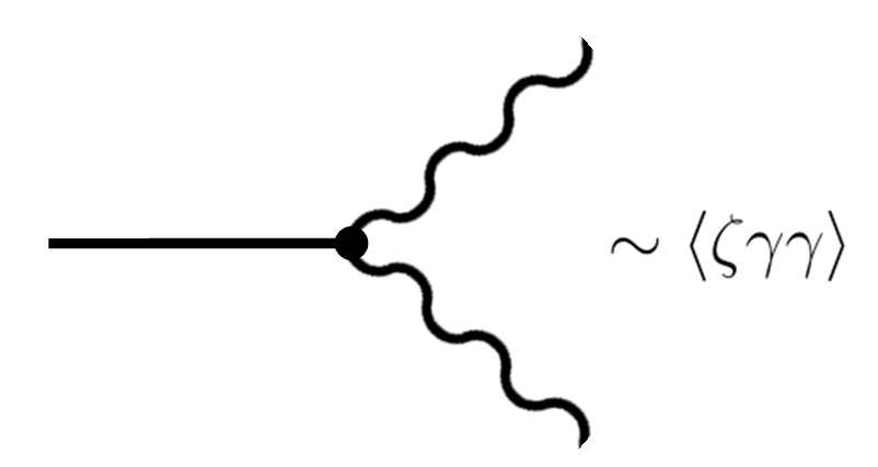
Figure 1: Three point vertex corresponding to inflaton-graviton-graviton (scalar-tensor-tensor) interaction. Gravitons are represented by wavy lines, the inflaton by the straight line.

There are several scenarios that will produce a classical coherent state for the inflaton following [46]. This can happen before the boost of for the case in which $|{\bf p}|\sim{\cal H}\ll|{\bf k}|\simeq|{\bf q}|$. This coherent state might be provided by a population of primordial Black Holes [47], e.g see eq A.4 of [39] taking a term like $\varphi J(t)$ where $J$ is a source of this coherent state of the inflaton. $J$ could be found, e.g., in the last line of eq. 3.8 of [45]. Another possibility is that the vacuum is not Bunch-Davies but a coherent state [48, 49, 50] (see also [51, 52]). More intuitively, all that is needed is a force in the inflaton potential, this could be given by a feature, or even the standard slow-roll.

3 Quantum nature, entanglement and Bell inequalities

In this section, we briefly review what is known to be the “most quantum aspect” in quantum mechanics and quantum optics: entanglement. This effect makes the quantum nature of a system appear in a very explicit manner; if we are hoping to find traces of quantumness in some observable, entanglement is what we should aim for.

3.1 Definition of entanglement

Entanglement between two quantum states is present when the quantum state describing the whole system cannot be written as a product of the states describing each subsystem separately, i.e. it is non-separable.
For the case of two particles which can be either in one-particle states $\ket{\psi_{1}}$ or $\ket{\psi_{2}}$, a general entangled state would the the superposed state:

$$\ket{\Psi}=\alpha\ket{\psi_{1}}_{1}\otimes\ket{\psi_{1}}_{2}+\beta\ket{\psi_{2}}_{1}\otimes\ket{\psi_{2}}_{2}$$ (3.1)

where $\alpha,\,\beta\in\mathbb{C}$, and $|\alpha|^{2}+|\beta|^{2}=1$. We note that $\ket{\psi_{i}}_{j}$ represents particle $j$ (the index $j$ could be a particle, momenta, directions, etc…]) in state $\ket{\psi_{i}}$.

Entanglement is exclusively a consequence of the principle of superposition present in quantum mechanics, and makes the non-locality of the theory explicit. Picture the following experiment:

One is to perform a measure of some observable $\mathcal{O}$ on the subsystem formed by particle 1 (for example, the same works if we start by measuring particle 2). This will result in the measure of one of the eigenvalues of the associated hermitic operator, for example $\lambda_{1}$, with probability $|\alpha|^{2}$, and the instantaneous collapse of the single-state of particle 1 to $\ket{\psi_{1}}$. If we look now at the 2-state describing the whole system, it will have instantaneously collapsed to its left term $\ket{\psi_{1}}_{1}\otimes\ket{\psi_{2}}_{2}$. In turn, this implies that from the moment particle 1 has been measured, particle 2 can only be in state $\ket{\psi_{2}}$, even if before the measurement on its companion, the state of particle 2 had contributions from both components $\psi_{1}$ and $\psi_{2}$. By performing a measure on 1 particle, we instantaneously change the state of the other.

This effect is instantaneous upon measurement of particle 1 regardless of the positions of each of the particles, and thus non-local.

3.2 Bell inequalities and experiment

In 1964, the physicist John Stewart Bell proposed his famous theorem [53], which showed a clear mathematical difference between any description by a classical, local hidden variables theory, or by the quantum-mechanical theory that gave rise to the non-local effect of entanglement. Extensive work has been done over the years concerning all theoretical and experimental aspects of Bell’s theorem and experiment [54, 55, 46, 56]. For the purpose of our work, we are interested in replicating each of the needed elements of the Bell experiment in our inflationary paradigm. These elements are [43]:

• Two separate spatial locations, call them Alice’s location and Bob’s location.

• An entangled state of the type (3.1), with components at these two locations.

• Two possible measurements of some physical observable, whose result is dependent on some local variable $\theta_{i}$ (or on some random choice between $\theta_{i}$ and $\theta_{i}^{\prime}$), at each of the spatial locations (denoted by $i=1,2$). Each observation/measurement is represented by non-commuting operators, call them $A(\theta_{1})$ and $A(\theta_{1}^{\prime})$, and $B(\theta_{2})$ and $B(\theta_{2}^{\prime})$, respectively.

• Definite results for the quantum measurement of the operators. For the inequality presented below, both $A(\theta_{1})$ and $B(\theta_{2})$ measured on the state (3.1) can yield $\pm 1$.

• A classical channel to transmit the results of the measurements to a common location where they can be correlated.

We can define the observable:

$$S=C(\theta_{1},\theta_{2})+C(\theta_{1}^{\prime},\theta_{2})+C(\theta_{1},\theta_{2}^{\prime})-C(\theta_{1}^{\prime},\theta_{2}^{\prime})$$ (3.2)

where $C(\theta_{1},\theta_{2})=\expectationvalue{A(\theta_{1})\,B(\theta_{2})}$. $S$ is such that in a description with a classical, local hidden variable theory (where the measure of $A$ is uncorrelated with the measure of $B$), $S^{\text{local hidden variables}}\leq 2$, while the quantum mechanical expectation value can be larger, $S^{\text{QM}}\leq 2\sqrt{2}$. By exceeding the former inequality in experimental measures, one proves the non-locality as an intrinsic property of entanglement and quantum mechanics. This particular Bell inequality is known as the Clauser-Horne-Shimony-Holt inequality [55].

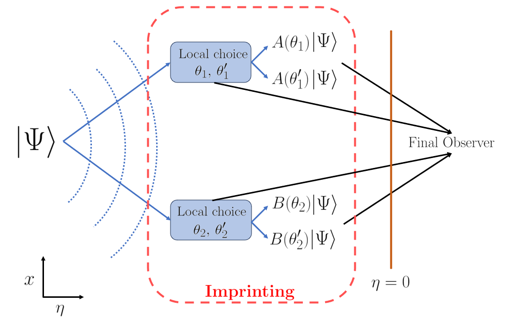
Figure 2: Set up for a Bell inequality violating experiment. The comoving time flows from left to right ($\eta=0$ represents the end of inflation), and spacial dimensions are drawn vertically. The entangled 2-state $\ket{\Psi}$ has components at two spatially-separate locations 1 (top) and 2 (bottom). Two different results of the measurement of observables $A$ and $B$ can be obtained, each dependent on the choice of the local variables $\theta_{1}$ and $\theta_{2}$, respectively. This choice is dependent on the interaction of the state with its local environment, it can be seen as a dependence on the measuring apparatus. The possible imprinting of the entanglement of state $\ket{\Psi}$ is represented by the dashed-line box. These results, together with the choices of $\theta_{i}$, are transmitted through classical channels (black arrows) to a final observer after inflation has finished.

3.3 Bell states

As we have seen, an entangled 2-state is generally of the form (3.1). It is useful to work with 2-states known as Bell states [46], which are defined as

$$\ket{\Psi_{\text{Bell}}^{\pm}}=\frac{1}{\sqrt{2}}(\ket{0}_{1}\ket{1}_{2}\pm\ket{1}_{1}\ket{0}_{2})\,,$$ (3.3)

$$\ket{\Phi_{\text{Bell}}^{\pm}}=\frac{1}{\sqrt{2}}(\ket{0}_{1}\ket{0}_{2}\pm\ket{1}_{1}\ket{1}_{2})\,.$$ (3.4)

Here, $\ket{0}_{i}$ and $\ket{1}_{i}$ represent the basis states of a general bipartite system (or two-mode system). The notation $\ket{i}_{1}\otimes\ket{j}_{2}$ denotes the tensor product of the basis states of subsystems 1 and 2, which define a basis of the Hilbert space $\mathcal{H}=\mathcal{H}_{1}\otimes\mathcal{H}_{2}$, in which two-particle states live.

4 Inflation as our laboratory

We have now all the necessary ingredients to design a plausible cosmological Bell-type experiment taking place during inflation. Some signature of violation of Bell inequalities, and therefore of the non-locality intrinsic to the quantum theory would allow us to prove the quantum mechanical origin of primordial in-homogeneities that gave rise to the observed large scale structure of our Universe. At least, this possible signature might serve as prove of concept for the theoretical scientific community, and serve as a possible observational path to follow by the experimental community.

4.1 Elements of the cosmological Bell experiment

We proceed to describe our realization of a cosmological Bell-type experiment in the inflationary epoch. For that we need a specific realization of the general elements described in section 3.2, and goes as follows:

• Alice’s and Bob’s locations will be two spatially separate points at the inflationary Hubble horizon, $H^{-1}_{\Lambda}\approx\text{constant}$, i.e., when the measurement of the polarization of the gravitons is performed, the momentum of the gravitons (when they are produced) should be around or greater than $\cal H$ and the momentum of Alice and Bob (i.e. related to the inverse of the dimensions of their ”laboratories”) should be much greater than that of the graviton.

• Our Bell state describes two gravitons entangled in their tensor polarizations, see section 4.2, eq. (4.4). Each graviton is at one of the spatial locations (Alice’s graviton and Bob’s graviton).

• The physical observable is the polarization of the gravitons, with two possible results $\theta_{i}\equiv P_{i}=+,\times$ (we could use also L and R polarizations depending on how Alice and Bob do the measurements.) The measure at each location is performed by the decoherence effect due to the gathering of “which-path information” by the cosmological horizon as described in [57, 58], see section 4.3.

• The possible results of the measurement (decoherence) of Alice’s and Bob’s gravitons are the $\times$ and $+$ polarizations of each graviton. In our case, the result would then leave an imprint through the interaction of two inflatons with the polarized local curvature (generated by the graviton). At each location Alice and Bob, we have scattering of two inflatons through graviton exchange (GE), as described in section 4.4 (see also [39] for a discussion on GE). We could say that both Alice and Bob use a pair of inflatons each to imprint the results of their measure of polarization.

• The result of the measure (or its imprint) is classically transmitted by the propagation of these pairs of scalar fluctuations (inflatons) after horizon crossing, where their amplitude freezes until the end of inflation, and then reenters during radiation epoch. Note that we have a non-trivial effect due to the derivatives on the two scalar fluctuations (se eq. 5.1 in [39]) this provides a non-trivial fingerprint that depends on the polarization of the graviton that Alice and/or Bob measured in their patch. The common location to which the results are transmitted is the range of scales set between the corresponding moments of reentering of Alice’s fluctuations and Bob’s fluctuations. Results can be correlated through the 4-point functions $\expectationvalue{\zeta_{\mathbf{k}_{1}}\zeta_{\mathbf{k}_{2}}\zeta_{\mathbf{k}_{3}}\zeta_{\mathbf{k}_{4}}}^{\text{GE}}_{\mathbf{A}}(P_{1})$, $\expectationvalue{\zeta_{\mathbf{k}_{1}}\zeta_{\mathbf{k}_{2}}\zeta_{\mathbf{k}_{3}}\zeta_{\mathbf{k}_{4}}}^{\text{GE}}_{\mathbf{B}}(P_{2})$

The derivatives on the scalar field fluctuations could leave an additional imprint on the two subhalos of each patch with the possibility that we could observe it on the large scale structure through the ’intrinsic alignment’. Note that this ’intrinsic alignment’ is obtained by performing the (perturbed Taylor) expansion between one subhalo with the second one in the same patch. In this case, the two derivatives are obtained for the same potential: i.e. a tidal effect between these two subhaloes linked to the polarization of the graviton.

In the following, we present a feasible way in which each of these elements appear in our inflationary setup.

4.2 Entangled state of gravitons

We start with the Hamiltonian (2.23). We now label the gravitons with momentum $-\mathbf{k}$ and $\mathbf{k}$ as gravitons 1 and 2, respectively. Following [46], and ignoring the left hand side of the tensor product in the Hamiltonian (pumping signal, corresponds to the destruction operator of the coherent inflaton field)

$$H_{\text{int}}^{(a\,b^{\dagger}b^{\dagger})}\equiv H_{I}\sim\left[\left(\hat{b}^{+}_{1}\right)^{\dagger}\left(\hat{b}^{+}_{2}\right)^{\dagger}-\left(\hat{b}^{\times}_{1}\right)^{\dagger}\left(\hat{b}^{\times}_{2}\right)^{\dagger}\right]+h.c.$$ (4.1)

We start from an initial vacuum state:

$$\ket{\Psi_{0}}=\ket{0}\equiv\ket{0}_{1}\otimes\ket{0}_{2}\equiv\ket{0}_{+,1}\ket{0}_{\times,1}\otimes\ket{0}_{+,2}\ket{0}_{\times,2}$$ (4.2)

where we have split the two vacua (for gravitons 1 and 2) in their “plus” and ‘cross” polarization components, i.e. we define the single states of each graviton (and its vacuum) in terms of these two components:

$$\ket{0}_{i}:=\ket{0}_{+,i}\ket{0}_{\times,i}\quad;\quad\ket{+}_{i}:=\ket{1}_{+,i}\ket{0}_{\times,i}\quad;\quad\ket{\times}_{i}:=\ket{0}_{+,i}\ket{1}_{\times,i}\quad;\quad(i=1,2)$$

We will discuss below the values for the momenta of the gravitons. Taking a first order approximation in the Schrödinger equation for the time evolution of the state:

$$\ket{\Psi(t)}=e^{-itH_{I}/\hbar}\ket{\Psi_{0}}\approx\left(1-\frac{it}{\hbar}H_{I}\right)\ket{0}\,\,\,,$$ (4.3)

where we expand the evolution operator to first order because: 1) we are considering instantaneous interactions and 2) to obtain the Bell state we consider very short inflaton interactions (in the coherent (classical) state) and the two gravitons. This leads to

$$\ket{\Psi(t)} \sim\ket{0}-\frac{it}{\hbar}\left(\ket{1}_{+,1}\ket{0}_{\times,1}\otimes\ket{1}_{+,2}\ket{0}_{\times,2}-\ket{0}_{+,1}\ket{1}_{\times,1}\otimes\ket{0}_{+,2}\ket{1}_{\times,2}\right)$$ (4.4)

$$=\ket{0}-\frac{it}{\hbar}\left(\ket{+}_{1}\ket{+}_{2}-\ket{\times}_{1}\ket{\times}_{2}\right)$$

$$\equiv\frac{it}{\hbar}\left(\ket{\times\times}-\ket{++}\right)$$

We can see that this state $\ket{\Psi}$ is proportional to the Bell state $\ket{\Phi^{-}_{\text{Bell}}}$ in (3.3).

4.3 The measure by the cosmological horizon

Once we have our entangled state of graviton polarizations $\ket{\Psi}$ of equation (4.4), we can proceed with the measurement of the state as part of the Bell experiment. The two gravitons need to be spatially separated. This is reasonable since they come from the inflaton “pump” (which we set in the CMF of $\zeta$ and got gravitons with $-\mathbf{k}$ and $\mathbf{k}$), and we can always boost them to a lab frame in which they are at an angle $2\alpha=\arccos\left[\left(E_{\zeta}/\sqrt{2}\,E_{\gamma}\right)^{2}-1\right]$ at the moment of creation. Here $E_{\zeta}$ and $E_{\gamma}=k$ are the energies of the inflaton and gravitons, respectively. Since teh boost is small for our reference frame, the change in energy is also negligible.

Now, in order to perform the measurement of our Bell state, we use the results in [57, 58]. In these works, it is suggested that in the presence of a Killing horizon, information from a quantum state in the vicinity of the horizon falls through it, and this decoheres the quantum superposition (or measures it). This Killing horizon can come from different objects, including the cosmological horizon intrinsic to de Sitter spacetime [58]. It could also be due to the presence of a population of primordial black holes during inflation [47]; also note that we are not in an exact de Sitter spacetime and that this symmetry (i.e. the existence of this Killing horizon) could be weakly broken.

This result comes from the fact that a massive object in a quantum superposition radiates a retarded gravitational field (soft gravitons). In Minkowski spacetime, for an inertial frame and imposing adiabatic evolution of the quantum state, decoherence can be avoided (a recombination of the spatially separated wave-packets of the superposed state can be performed in a way such that no information is lost, see [57]). However, in the presence of a Killing horizon like the cosmological horizon of inflation, part of this radiated field inevitably falls through the horizon. In this way, as time passes the horizon gathers “which-path information” about the quantum superposition, decohering (measuring) more and more the state. This decoherence is expressed as:

$$\mathcal{D}=1-\innerproduct{\psi_{1}}{\psi_{2}}_{H_{\Lambda}^{-1}}=1-e^{-\frac{1}{2}\expectationvalue{N}}$$ (4.5)

where $\expectationvalue{N}$ represents the average number of soft gravitons (gravitational field) that are radiated through the horizon and $\ket{\psi_{1}},\,\ket{\psi_{2}}$ represent the quantum states of the radiated gravitational field sourced by the object in a spatial quantum superposition, in our case each graviton at locations $A$ and $B$:

$$\ket{\Psi}\sim\frac{1}{\sqrt{2}}\left(\ket{\{\times\,\text{or}\,+\}}_{A}+\ket{\{\times\,\text{or}\,+\}}_{B}\right)\equiv\frac{1}{\sqrt{2}}\left(\ket{\psi_{1}}+\ket{\psi_{2}}\right)$$ (4.6)

In Eq. (4.5) $\innerproduct{\psi_{1}}{\psi_{2}}_{H_{\Lambda}^{-1}}$ is the inner product (defined in [57]) of the 1-particle states of the soft gravitons falling through the horizon $H_{\Lambda}^{-1}$. Note that the massive quantum particle that is subjected to decoherence has “somewhere” imprinted the information of the polarization of the graviton discussed previously.

One issue that arises is the fact that gravitons are massless. We will deal with this in sec. 4.4. For now, we take that decoherence occurs through the gathering of “which-path information” by the cosmological horizon. Let us detail how exactly decoherence happens. There are two options, both leading to an “effective measurement” of the polarization:

1. The entangled 2-state decoheres as a whole to only one of the superposed states, e.g.

   $$\ket{\Psi}\sim\ket{\times\times}-\ket{++}\overset{\mathcal{D}}{\longrightarrow}\ket{\times\times}\,\,,$$

   which is something desirable, because it collapses our polarizations to one possibility only.
   

2. The decoherence occurs separately on the superposed states of one graviton (or both) (e.g. Alice’s graviton):

   $$\ket{\psi}_{A}\sim\ket{\{\times\text{ or }+\}}_{A}\overset{\mathcal{D}_{A}}{\longrightarrow}\ket{\times}_{A}\,\,,$$

   which, if (some) coherence of the entangled 2-state is maintained, would automatically force Bob’s graviton to $\ket{\times}_{B}$.
   

The right hand term in the second equality of Eq. (4.5) contains $\expectationvalue{N}$, which represents the average number of soft gravitons (gravitational field) that are radiated through the horizon. In the case of a cosmological horizon, we have [58]:

$$\expectationvalue{N}\sim\frac{m^{2}d^{4}}{R_{H}^{5}}\,T\,\,,$$ (4.7)

where $R_{H}=H_{\Lambda}^{-1}$ is the cosmological horizon radius, $m$ is the mass of the superposed quantum object (see sec. 4.4), $d$ is the spatial separation between the two wavepackets Alice and Bob, and $T$ is the proper time for which the mass has been radiating soft gravitons that fall through the horizon. Note that the lab A is at the worldline $r=0$ (inertial orbit of the static Killing field), being the horizon at $r=R_{H}$. Alice and Bob should be in opposite directions at a distance given by 4.9. This is true for our gravitons with comoving wavenumber $k$, since they where created at the same spatial location which we take it to be $r=0$, and in comoving coordinates are in an inertial frame.

This leads to a decoherence time (in natural units):

$$T_{D}\sim\frac{R_{H}^{5}}{m^{2}d^{4}}\,\,.$$ (4.8)

The proper distance $d$ around the time of horizon crossing can be estimated as:

$$d\approx 2R_{H}\sin\alpha\approx 2R_{H}\sin\left(\frac{1}{2}\,\arccos\left[\left({E_{\zeta}}/{\sqrt{2}\,k}\right)^{2}-1\right]\right)\,\,.$$ (4.9)

Now, under the decoherence/measurement induced by the cosmological horizon, the polarization of both gravitons will be (partially) forced to the same result of the measure, either $\times$ or $+$ polarization, right before horizon crossing.

4.4 Imprinting - scattering of inflatons by polarized graviton exchange at horizon crossing

Let us now hint a possible way in which the measure of the entangled state of gravitons might leave an imprint on a physical observable after inflation. This imprinting should happen right before horizon crossing, so that after becoming super-horizon the amplitude of fluctuations freezes and is classically preserved until its reentering into our Hubble horizon.

As we saw, we can use decoherence by the cosmological horizon as a measuring apparatus, as long as we have some mass associated to each graviton. We suggest that this effective mass comes from the Lagrangian and will enable the imprinting of the non-locality of the entangled state.

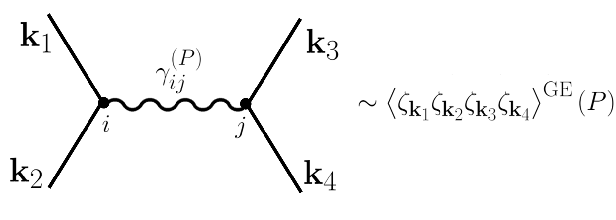
Figure 3: Graviton exchange of four inflatons [30]. Process of measure-imprinting at horizon crossing. The graviton is entangled with its partner, as described in the text. Note that the graviton on the diagram is in fact the two soft gravitons.

Take the four-point correlation function between scalar fluctuations (inflatons) mediated by graviton exchange (GE), depicted in Fig. 4. As shown in [30] the graviton exchange can be manifested as a measurable signal in the halo bias. In the calculation of the scattering amplitude of the shown Feynman diagram of Fig. 3, performed in [59] and used in [30], the sum over all possible polarizations of the graviton is taken, as is standard in QFT calculations when the polarization of the exchanged particle (graviton in this case) is unknown. The polarization of the graviton taking part in the GE is known and contained in the fig. 3 and therefore the overall scattering amplitude might be different. This then could have an effect on $\expectationvalue{\zeta_{\mathbf{k}_{1}}\zeta_{\mathbf{k}_{2}}\zeta_{\mathbf{k}_{3}}\zeta_{\mathbf{k}_{4}}}^{\text{GE}}(P)$, where $P$ represents the polarization of the exchanged graviton. We can think of this scattering as two inflatons which, at the time right before horizon crossing, feel some local curvature generated by the mediating graviton. Since the tensor polarizations correspond to the directions in which these local spacetime oscillations occur, $+$ and $\times$, one can picture a qualitative difference when the scattered inflatons “feel” this oscillatory feature.

We suggest that it is the mass of the incoming inflatons right around the time of the graviton exchange that gives an effective mass to the graviton so that it can radiate soft gravitons that fall through the horizon $H_{\Lambda}^{-1}$, and make it decohere through the mechanism presented in the previous section. For decoherence to become effective while the GE occurs, the time of decoherence should be comparable with the characteristic time scale of gravitation, for example if

$$T_{D}\sim t_{\text{GE}}\sim\frac{1}{M_{\text{Pl}}}\,\,.$$ (4.10)

From Eqs. (4.8, 4.9) and 4.10, taking comoving distance in comoving coordinates $\tilde{d}=d/a(\eta)$ and conformal time $\eta=T/a(\eta)$, and substituting $a(\eta)=R_{H}/\eta$ at the time around horizon crossing $|\eta|\sim k^{-1}$ for a mode of fixed comoving wavenumber $k$, we obtain the following relation (besides order one factors):

$$k_{D}\sim\left(\frac{m^{2}}{M_{\text{Pl}}\,R_{H}^{5}}\right)^{1/4}\sim\left(\frac{m^{2}}{M_{\text{Pl}}}\right)^{1/4}\,H_{\Lambda}^{5/4}$$ (4.11)

As mentioned, the effective mass of the decohering graviton would be twice the mass of the incoming inflatons, i.e. $m\equiv m_{\text{eff}}^{(\gamma)}\approx m^{(\zeta)}_{1}+m^{(\zeta)}_{2}$. $k_{D}$ represents the modes that upon arrival of the two inflatons, would decohere right before horizon crossing. Taking $m\sim 10^{-3}M_{\text{Pl}}$ and $H_{\Lambda}\sim\varepsilon_{\Lambda}^{1/2}$, yields:

$$k\sim 10^{-3/2}\varepsilon_{\Lambda}^{5/8}\ll 1$$ (4.12)

This number is expected to be small, and thus the modes that decohere while the GE takes place and could imprint the gravitons polarization are those corresponding to large scales. Also note that the graviton could decohere also with Hawking radiation.

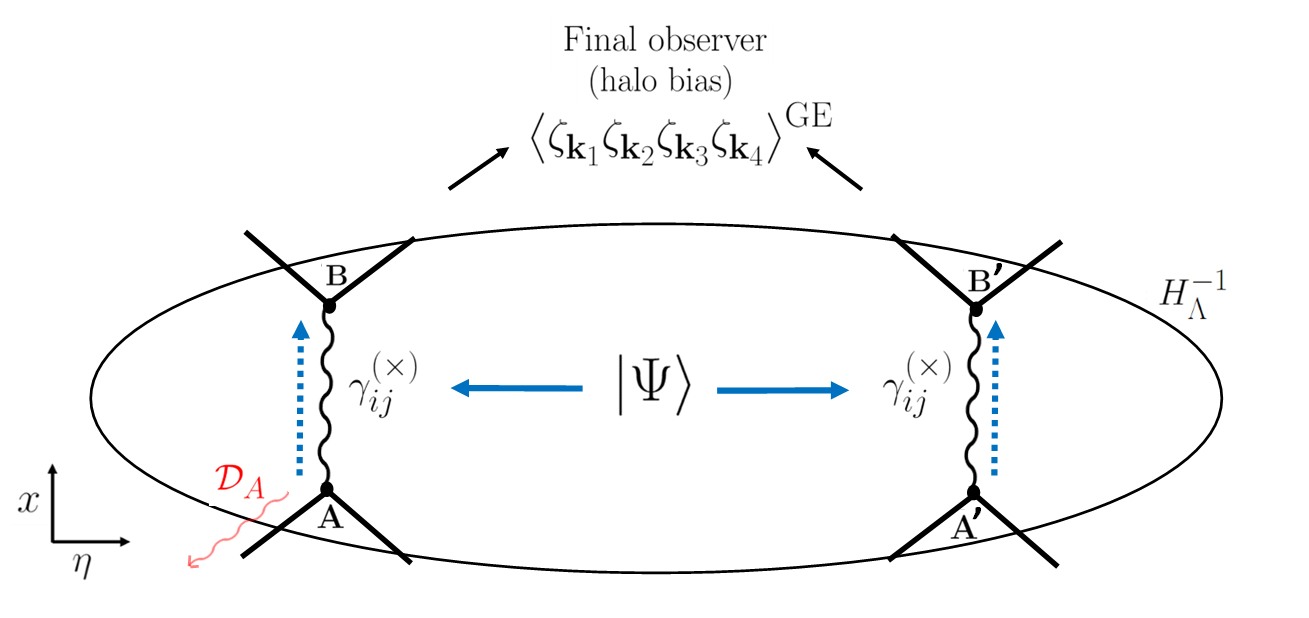
Figure 4: Schema of the imprinting process described in Sec. 4.3 and 4.4. The entangled state (in graviton polarizations) $\ket{\Psi}$ is transmitted to two separate spatial locations. Around the time of horizon crossing, two inflatons arrive and give some effective mass to each graviton while undergoing scattering by GE. This effective mass produces the radiation of soft gravitons (represented by the red, wavy line) through the horizon $H_{\Lambda}^{-1}$, and makes the entangled state decohere. This is represented for the case of graviton A, by $\mathcal{D}_{A}$, which collapses to $\times$ polarization. The blue, dotted arrow represents the instantaneous effect of collapse to $\times$ polarization of graviton $B$ due to the entanglement. This effect then remains on the 4-point function $\expectationvalue{\zeta_{\mathbf{k}_{1}}\zeta_{\mathbf{k}_{2}}\zeta_{\mathbf{k}_{3}}\zeta_{\mathbf{k}_{4}}}^{\text{GE}}_{\mathbf{A,B}}$. The fluctuations freeze after horizon crossing, and classically transmit this “spatial preference” (from polarization preference) to a final “observer” after the end of inflation ($\eta=0$). In our case, this final observer could be the correlation between 4-point functions $A$ and $B$ in the halo bias (calculated in [30]).

Let as now put together this possible imprinting with the fact that the graviton taking part in the GE has an entangled partner. Concretely, imagine that Alice’s graviton decoheres because of the which-path information obtained by the cosmological horizon i.e. $\mathcal{D}_{A}>0$, and collapses to “cross” polarization, $\times$. Now, only the “cross” term will contribute to the GE correlation through Alice’s graviton, $\expectationvalue{\zeta_{\mathbf{k}_{1}}\zeta_{\mathbf{k}_{2}}\zeta_{\mathbf{k}_{3}}\zeta_{\mathbf{k}_{4}}}^{\text{GE}}_{\mathbf{A}}(\times)$. And more importantly, from the moment $\mathcal{D}_{A}$ has become effective, some other scattering of two new inflatons through GE of Bob’s graviton will undergo exactly the same effect, i.e. only $\expectationvalue{\zeta_{\mathbf{k}_{1}}\zeta_{\mathbf{k}_{2}}\zeta_{\mathbf{k}_{3}}\zeta_{\mathbf{k}_{4}}}^{\text{GE}}_{\mathbf{B}}(\times)$ will contribute. In this way, because of the fact that there was an entangled 2-state between gravitons A and B, a spatial preference could have been formed. This preference would not have been there if our theory had preserved locality, or if we did not have an entangled state. This is shown in Fig. 4.

Let us interpret this process as follows: If we think that the “graviton” in Fig. 3 is, in reality our two gravitons that are emitted in two different directions to lab Alice and lab Bob, then the two Feymann diagrams are in reality the two measures that we need to do for each lab, i.e., where we will do a measure and they will be in the two sub-halos of patch A(lice) and B(ob).

5 Conclusions

We have presented a mechanism during the inflation period to generate entangled states of gravitons using the inflaton field as a “pump”. This entangled states can then be measured at a killing horizon, thus resulting in a observational feature of quantumness in the early Universe. Note that our effect is due to second order effects; we have a non-trivial effect due to the derivatives on the two scalar fluctuations and this provides a fingerprint that depends on the polarization of the graviton that Alice and/or Bob measured in their patch. We have proposed possible signatures in the halo bias due to graviton exchange, but it is also possible to speculate that this signature could manifest in the intrinsic alignment of galaxies or influence the spin of black holes if a primordial population exists during inflation. We will quantify the observational signatures in a future publication.

References

- [1] Viatcheslav F. Mukhanov and G. V. Chibisov. Quantum Fluctuations and a Nonsingular Universe. JETP Lett., 33:532–535, 1981.
- [2] Alan H. Guth and S. Y. Pi. Fluctuations in the New Inflationary Universe. Phys. Rev. Lett., 49:1110–1113, 1982.
- [3] S. W. Hawking. The Development of Irregularities in a Single Bubble Inflationary Universe. Phys. Lett. B, 115:295, 1982.
- [4] James M. Bardeen, Paul J. Steinhardt, and Michael S. Turner. Spontaneous Creation of Almost Scale - Free Density Perturbations in an Inflationary Universe. Phys. Rev. D, 28:679, 1983.
- [5] V. Mukhanov. Physical Foundations of Cosmology. Cambridge University Press, Oxford, 2005.
- [6] M. S. Turner E. W. Kolb. The Early Universe. Westview Press, 1990.
- [7] David Campo and Renaud Parentani. Space-time correlations in inflationary spectra: A Wave-packet analysis. Phys. Rev. D, 70:105020, 2004.
- [8] David Campo and Renaud Parentani. Space-time correlations within pairs produced during inflation, a wave packet analysis. Phys. Rev. D, 67:103522, 2003.
- [9] David Campo and Renaud Parentani. Inflationary spectra and violations of Bell inequalities. Phys. Rev. D, 74:025001, 2006.
- [10] David Campo and Renaud Parentani. Quantum correlations in inflationary spectra and violation of bell inequalities. Braz. J. Phys., 35:1074–1079, 2005.
- [11] David Campo, Jens C. Niemeyer, and Renaud Parentani. Damped corrections to inflationary spectra from a fluctuating cutoff. Phys. Rev. D, 76:023513, 2007.
- [12] David Campo and Renaud Parentani. Decoherence and entropy of primordial fluctuations. I: Formalism and interpretation. Phys. Rev. D, 78:065044, 2008.
- [13] David Campo and Renaud Parentani. Decoherence and entropy of primordial fluctuations II. The entropy budget. Phys. Rev. D, 78:065045, 2008.
- [14] Sayantan Choudhury, Sudhakar Panda, and Rajeev Singh. Bell violation in the Sky. Eur. Phys. J. C, 77(2):60, 2017.
- [15] Sayantan Choudhury, Sudhakar Panda, and Rajeev Singh. Bell violation in primordial cosmology. Universe, 3(1):13, 2017.
- [16] Sugumi Kanno. A note on initial state entanglement in inflationary cosmology. EPL, 111(6):60007, 2015.
- [17] Jerome Martin and Vincent Vennin. Quantum Discord of Cosmic Inflation: Can we Show that CMB Anisotropies are of Quantum-Mechanical Origin? Phys. Rev. D, 93(2):023505, 2016.
- [18] Sugumi Kanno and Jiro Soda. Bell Inequality and Its Application to Cosmology. Galaxies, 5(4):99, 2017.
- [19] Jerome Martin and Vincent Vennin. Obstructions to Bell CMB Experiments. Phys. Rev. D, 96(6):063501, 2017.
- [20] Jerome Martin and Vincent Vennin. Observational constraints on quantum decoherence during inflation. JCAP, 05:063, 2018.
- [21] Jérôme Martin and Vincent Vennin. Non Gaussianities from Quantum Decoherence during Inflation. JCAP, 06:037, 2018.
- [22] Sugumi Kanno. Nonclassical primordial gravitational waves from the initial entangled state. Physical Review D, 100(12), December 2019.
- [23] Sugumi Kanno and Jiro Soda. Polarized initial states of primordial gravitational waves, 2020.
- [24] Daine L. Danielson, Gautam Satishchandran, and Robert M. Wald. Gravitationally mediated entanglement: Newtonian field versus gravitons. Phys. Rev. D, 105(8):086001, 2022.
- [25] Thomas Colas, Julien Grain, and Vincent Vennin. Quantum recoherence in the early universe. EPL, 142(6):69002, 2023.
- [26] Kartik Prabhu, Gautam Satishchandran, and Robert M. Wald. Infrared finite scattering theory in quantum field theory and quantum gravity. Phys. Rev. D, 106(6):066005, 2022.
- [27] Aoumeur Daddi Hammou and Nicola Bartolo. Cosmic decoherence: primordial power spectra and non-Gaussianities. JCAP, 04:055, 2023.
- [28] Sirui Ning, Chon Man Sou, and Yi Wang. On the decoherence of primordial gravitons. Journal of High Energy Physics, 2023(6), June 2023.
- [29] Jerome Martin and Vincent Vennin. Quantum discord of cosmic inflation: Can we show that cmb anisotropies are of quantum-mechanical origin? Physical Review D, 93(2), January 2016.
- [30] Nicola Bellomo, Nicola Bartolo, Raul Jimenez, Sabino Matarrese, and Licia Verde. Measuring the energy scale of inflation with large scale structures. Journal of Cosmology and Astroparticle Physics, 2018(11):043?043, November 2018.
- [31] E. Calzetta and B. L. Hu. Quantum fluctuations, decoherence of the mean field, and structure formation in the early universe. Phys. Rev. D, 52:6770–6788, 1995.
- [32] Fernando C. Lombardo and Diana Lopez Nacir. Decoherence during inflation: The Generation of classical inhomogeneities. Phys. Rev. D, 72:063506, 2005.
- [33] Patrick Martineau. On the decoherence of primordial fluctuations during inflation. Class. Quant. Grav., 24:5817–5834, 2007.
- [34] Claus Kiefer, Ingo Lohmar, David Polarski, and Alexei A. Starobinsky. Pointer states for primordial fluctuations in inflationary cosmology. Class. Quant. Grav., 24:1699–1718, 2007.
- [35] Claus Kiefer and David Polarski. Why do cosmological perturbations look classical to us? Adv. Sci. Lett., 2:164–173, 2009.
- [36] Elliot Nelson. Quantum Decoherence During Inflation from Gravitational Nonlinearities. JCAP, 03:022, 2016.
- [37] C. P. Burgess, R. Holman, G. Tasinato, and M. Williams. EFT Beyond the Horizon: Stochastic Inflation and How Primordial Quantum Fluctuations Go Classical. JHEP, 03:090, 2015.
- [38] D. Boyanovsky. Effective field theory during inflation: Reduced density matrix and its quantum master equation. Phys. Rev. D, 92(2):023527, 2015.
- [39] C.P. Burgess, R. Holman, Greg Kaplanek, Jerome Martin, and Vincent Vennin. Minimal decoherence from inflation. Journal of Cosmology and Astroparticle Physics, 2023(07):022, July 2023.
- [40] Chon Man Sou, Duc Huy Tran, and Yi Wang. Decoherence of cosmological perturbations from boundary terms and the non-classicality of gravity. JHEP, 04:092, 2023.
- [41] Hael Collins and Tereza Vardanyan. Entangled scalar and tensor fluctuations during inflation. Journal of Cosmology and Astroparticle Physics, 2016(11):059?059, November 2016.
- [42] Jinn-Ouk Gong and Min-Seok Seo. Quantum non-linear evolution of inflationary tensor perturbations. JHEP, 05:021, 2019.
- [43] Juan Maldacena. A model with cosmological bell inequalities. Fortschritte der Physik, 64(1):10–23, dec 2015.
- [44] Mukhanov. Introduction to Quantum Effects in Gravity. Cambridge University Press, 2007.
- [45] Juan Martin Maldacena. Non-Gaussian features of primordial fluctuations in single field inflationary models. JHEP, 05:013, 2003.
- [46] P. L. Knight C. Gerry. Introductory Quantum Optics. Cambrige University Press, 2004.
- [47] Tsvi Piran and Raul Jimenez. Black holes as ?time capsules?: A cosmological graviton background and the hubble tension. Astronomische Nachrichten, 344(1?2), January 2023.
- [48] Alexander m. Polyakov. PHASE TRANSITIONS AND THE UNIVERSE. Sov. Phys. Usp., 25:187, 1982.
- [49] Ignatios Antoniadis, Pawel O. Mazur, and Emil Mottola. Cosmological dark energy: Prospects for a dynamical theory. New J. Phys., 9:11, 2007.
- [50] Gia Dvali, Cesar Gomez, and Sebastian Zell. Quantum Break-Time of de Sitter. JCAP, 06:028, 2017.
- [51] Sandipan Kundu. Inflation with General Initial Conditions for Scalar Perturbations. JCAP, 02:005, 2012.
- [52] Houri Ziaeepour. Quantum coherent states in cosmology. J. Phys. Conf. Ser., 626(1):012034, 2015.
- [53] J. S. Bell. On the einstein podolsky rosen paradox. Physics Physique Fizika, 1:195–200, Nov 1964.
- [54] A. Shimony J. F. Clauser. Bell’s theorem. experimental tests and implications. Rep. Prog. Phys. 41 1881, 1978.
- [55] John F. Clauser, Michael A. Horne, Abner Shimony, and Richard A. Holt. Proposed experiment to test local hidden-variable theories. Phys. Rev. Lett., 23:880–884, Oct 1969.
- [56] D. F. Walls and Gerard J. Milburn. Quantum Optics. 2008.
- [57] Daine L. Danielson, Gautam Satishchandran, and Robert M. Wald. Black holes decohere quantum superpositions. International Journal of Modern Physics D, 31(14), July 2022.
- [58] Daine L. Danielson, Gautam Satishchandran, and Robert M. Wald. Killing horizons decohere quantum superpositions. Physical Review D, 108(2), July 2023.
- [59] David Seery, Martin S Sloth, and Filippo Vernizzi. Inflationary trispectrum from graviton exchange. Journal of Cosmology and Astroparticle Physics, 2009(03):018?018, March 2009.