Identifiable Latent Neural Causal Models
Abstract
Causal representation learning seeks to uncover latent, high-level causal representations from low-level observed data. It is particularly good at predictions under unseen distribution shifts, because these shifts can generally be interpreted as consequences of interventions. Hence leveraging seen distribution shifts becomes a natural strategy to help identifying causal representations, which in turn benefits predictions where distributions are previously unseen. Determining the types (or conditions) of such distribution shifts that do contribute to the identifiability of causal representations is critical. This work establishes a sufficient and necessary condition characterizing the types of distribution shifts for identifiability in the context of latent additive noise models. Furthermore, we present partial identifiability results when only a portion of distribution shifts meets the condition. In addition, we extend our findings to latent post-nonlinear causal models. We translate our findings into a practical algorithm, allowing for the acquisition of reliable latent causal representations. Our algorithm, guided by our underlying theory, has demonstrated outstanding performance across a diverse range of synthetic and real-world datasets. The empirical observations align closely with the theoretical findings, affirming the robustness and effectiveness of our approach.
1 Introduction
Causal representation learning offers the promise of discerning the pivotal latent variables that dictate a system’s behavior, along with the intricate causal relationships among them (Schölkopf et al., 2021). A main advantage of causal representations is their ability to facilitate predictions under unseen distribution, a constant challenge to most machine learning algorithms yet a frequent phenomenon in real-world data, particularly in fields like medical imaging (Chandrasekaran et al., 2021), biogeography (Pinsky et al., 2020), and finance (Gibbs & Candes, 2021). The advantage of causal representations stems from the understanding that distribution shifts are often the result of interventions. Specifically, interventions bring about changes in the fundamental causal influences among causal variables within a system, leading to distribution shifts (Peters et al., 2017; Pearl, 2000; Spirtes et al., 2001).
The foundational theories of causal representation learning, especially the aspect of identifiability which focuses on the uniqueness of causal representations, present a complex and nuanced challenge. Given that the main advantage of causal representations is making predictions under unseen distribution shifts as mentioned above, it seems natural to investigate the identifiability of causal representations through observed (e.g., seen) distribution shifts. When delving into the use of seen distribution shifts for the identifiability, it is crucial to first acknowledge that distribution shifts primarily stem from self-initiated behaviors within a causal system across diverse environments, due to the inherent unobservability of latent causal variables.
The critical question that arises when leveraging distribution shifts for the identifiability of causal representations, is: what types of distribution shifts contribute to identifiability? There are primarily two categories for modeling distribution shifts: those arising from hard interventions (Brehmer et al., 2022; Ahuja et al., 2023; Seigal et al., 2022; Buchholz et al., 2023; Varici et al., 2023), and those arising from soft interventions (Liu et al., 2022, 2023). Hard interventions, while valuable for enabling nonparametric latent causal models, necessitate that the self-initiated behaviors within a causal system fall within the scope of specific types of distribution shifts. This can be a limitation as these behaviors generally tend to be somewhat arbitrary. Identifying causal representations through hard interventions is thus somewhat limited. On the contrary, soft interventions align with a wider range of potential distribution shifts Liu et al. (2022, 2023), offering a more flexible way for modeling self-initiated behaviors. Note that, although Liu et al. (2022) takes a step in this direction, it focuses on characterizing distribution shifts within latent linear models, which may have limited relevance when applied to real-world applications. Similarly, the work in Liu et al. (2023) characterizes types of distribution shifts in latent polynomial models, well known for their universal approximation capabilities, but polynomial models are susceptible to issues such as numerical instability and exponential growth in terms. Given space constraints, we defer a more comprehensive discussion of related work to in Appendix A.
This work aims to investigate the types of distribution shifts suitable for identifying causal representations within general latent additive noise models. It thus encompasses both latent linear models in Liu et al. (2022) and latent polynomial models in Liu et al. (2023). Importantly, additive noise models, particularly when implemented through Multilayer Perceptrons (MLPs), offer significantly greater flexibility than polynomial models while also addressing the other limitations mentioned above. By introducing a sufficient and necessary condition upon the types of distribution shifts, we show that latent additive noise causal models can be identified up to trivial permutation transformation with scaling, under certain assumptions introduced by nonlinear ICA (Hyvarinen & Morioka, 2016; Hyvarinen et al., 2019; Khemakhem et al., 2020; Sorrenson et al., 2020). In addition, we consider practical scenarios where only a subset of data with distribution shifts is obtainable, and provide partial identifiability results. Furthermore, we generalize the identfiability result of latent latent additive noise causal models to latent post-nonlinear causal models, which are a more general framework that encompasses additive noise models as a special case. To validate our findings, we have developed a novel method for learning latent additive noise causal models. Our empirical experiments on synthetic data, image data, and real fMRI data serve to demonstrate the effectiveness of our proposed approach, and align closely with the identifiability results.
2 Identifiable Latent Additive Noise Models by Leveraging Distribution Shifts
In this section, we show that by leveraging distribution shifts, latent additive noise models with noise sampled from two-parameter exponential causal representations are identifiable, which also implies that the corresponding latent causal structures can be recovered. We begin by introducing our defined latent additive noise causal models in Section 2.1, aiming to facilitate comprehension of the problem setting and highlight our contributions. Following this, in Section 2.2, we present our identifiability result by establishing a sufficient and necessary condition that characterizes the types of distribution shifts, thereby achieving identifiability. These results extend beyond previous identifiability findings in both linear models (Liu et al., 2022) and polynomial models (Liu et al., 2023). We, additionally, show partial identifiability results, addressing scenarios where only a portion of distribution shifts is available. This exploration narrows the gap between our findings and practical applications.
2.1 Latent Additive Noise Models with Distribution Shifts
In our investigation, we explore the following latent causal generative models that elucidate the underlying processes. Within these models, the observed data, represented as , is generated through latent causal variables denoted as (where ). Furthermore, these latent causal variables are generated by combining latent noise variables , known as exogenous variables in causal systems, and the causal graph structure among latent causal variables. Unlike previous works that necessitate specific graph structures, we do not impose any restrictions on the graph structures among latent causal variables other than acyclicity. In addition, we introduce a surrogate variable to characterize distribution shifts by modeling the changes in the distribution of , as well as the causal influences among latent causal variables . Here could be thought of as environment index. More specifically, we parameterize the causal generative models by assuming follows an exponential family given , and assuming and are generated as follows:
| (1) | ||||
| (2) | ||||
| (3) |
where
-
•
in Eq. (1), denotes the normalizing constant, and denotes the sufficient statistic for , whose natural parameter depends on . Here we focus on two-parameter (e.g., ) exponential family members, e.g., Gaussian, inverse Gaussian, Gamma, inverse Gamma, and beta distributions as special cases.
-
•
In Eq. (2), the term represents the set of parents of . signifies a mapping, which can take on various forms, including both linear and nonlinear mappings. In addition, there exist common Directed Acyclic Graphs (DAG) constraints among latent causal variables .
-
•
In Eq. (3), denotes a nonlinear mapping, and is independent noise with probability density function .
The proposed latent additive noise models can encompass two specific model types: latent linear Gaussian models as presented in (Liu et al., 2022), and latent polynomial models as introduced in Liu et al. (2023). More specifically, when we constrain Eq. (1) to follow a Gaussian distribution and restrict the mapping in Eq. (2) to linear transformations, our latent additive noise models effectively transform into the latent linear Gaussian models described in Liu et al. (2022). Similarly, when we limit the mapping in Eq. (2) to polynomial functions, our latent additive noise models are then reduced to the latent polynomial models discussed in (Liu et al., 2023). Furthermore, despite the approximation capabilities of polynomial models (Liu et al., 2023), they are susceptible to issues such as numerical instability and exponential growth in terms. This is especially serious when one needs high-degree terms to more accurately approximate complex relations among latent causal variables, particularly when the dimensionality of latent causal variables is high. By contrast, the proposed latent additive noise models, especially when implemented through Multilayer Perceptrons (MLPs), offer significantly greater flexibility than polynomial models for addressing the limitations inherent in polynomial models.
2.2 Complete Identifyability Result
One of our primary contributions involves harnessing distribution shifts resulting from self-initiated behaviors within a causal system to enhance the identifiability of causal representations. Unlike many prior studies that restrict distribution shifts to the specific context of hard interventions (Brehmer et al., 2022; Ahuja et al., 2023; Seigal et al., 2022; Buchholz et al., 2023; Varici et al., 2023), our focus extends to a broader spectrum of potential distribution shifts associated with soft interventions. Additionally, while Liu et al. (2022) explore soft interventions in limited latent linear Gaussian models, and Liu et al. (2023) investigate them in latent polynomial models, both of them encounter issues such as numerical instability and exponential growth, our approach delves into soft interventions within additive noise models, which encompass the two specific model types mentioned earlier. The model capabilities of the proposed latent additive noise models enable more generalized identifiability results as follows:
Theorem 2.1.
Suppose latent causal variables and the observed variable follow the causal generative models defined in Eqs. 1 - 3. Assume the following holds:
-
(i)
The set has measure zero, where is the characteristic function of the density ,
-
(ii)
The function in Eq. 3 is injective,
-
(iii)
There exist values of , i.e., , such that the matrix
(4) of size is invertible. Here ,
-
(iv)
The function class of satisfies the following condition: for each parent node of , there exist constants , such that ,
then the true latent causal variables are related to the estimated latent causal variables , which are learned by matching the true marginal data distribution , by the following relationship: where denotes the permutation matrix with scaling, denotes a constant vector.
Assumptions (i)-(iii) are orignally deveoloped by nonlinear ICA (Hyvarinen & Morioka, 2016; Hyvarinen et al., 2019; Khemakhem et al., 2020; Sorrenson et al., 2020). We here consider unitizes these assumptions considering the following two main reasons. 1) These assumptions have been verified to be practicable in diverse real-world application scenarios (Kong et al., 2022; Xie et al., 2022b; Wang et al., 2022). 2) Our result eliminates the need to make assumptions about the dimensionality of latent causal or noise variables, which is in contrast to existing methods that require prior knowledge of the dimensionality, due to imposing the two-parameter exponential family members on latent noise variables (Sorrenson et al., 2020).
Assumption (iv), originally introduced by this work, is to offer a sufficient and necessary condition, which characterizes the various types of distribution shifts within the context of general latent additive noise models, contributing to identifiability. Assumption (iv), for instance, could arise in the analysis of cell imaging data, where contexts involve cell batches exposed to different small-molecule compounds. In this setting, each latent variable denotes the protein group concentration (Chandrasekaran et al., 2021). Small molecules pose challenges due to varying mechanisms of action, affecting selectivity (Forbes & Krueger, 2019).
Note that: 1) assumption (iv) is intended to constrain the function class of and does not necessitate the availability of observed data corresponding to the specific . 2) assumption (iv) is general version of corresponding assumption (v) in latent linear models in Liu et al. (2022) and assumption (iv) in latent polynomial models in Liu et al. (2023). In addition, assumption (iv) have two significant implications. 1) It indicates that not all distribution shifts in the context of latent additive noise models contribute to identifiability. 2) It defines a boundary within the domain of latent additive noise models, distinguishing which types of distribution shifts are beneficial for identifiability and which are not. Let us consider the following simple example for further clarity for these two implications.
Example:
For simplicity, let us parameterize Eq. (2) as follows (let be a parent of ): . In this case, consider that can be replaced as . As a consequence, while the distribution of shifts across , there always exists a team that remains unchanged across . Importantly, the unchanged term across can be absorbed into , the mapping from to , resulting in the form , not the groundturth , which leads to an unidentifiable outcome. A rigorous justification will be provided in Section 2.3. This demonstrates that not all distribution shifts contribute to identifiability. Moreover, in the parametric case described above, condition (iv) implies that we require and , which results in that can not include a non-zero constant term and thus cannot be replaced by with . Therefore, condition (iv) defines a boundary between the types of distribution shifts that contributes to identifiability and those that do not.
Proof sketch
The proof can be done according to the following intuition. With the support of assumptions (i)-(iii), one can utilize the identifiability result from nonlinear ICA to identify the latent noise variables up to permutation and scaling, e.g., where denotes the recovered latent noise variables obtained by matching the true marginal data distribution. This outcome, in conjunction with the definition in (2), facilitates the establishment of a mapping between the the true latent causal variables and the recovered latent causal variables , e.g., . Finally, by showing that the Jacobian matrix of is equivalent to if and only if condition (iv) is satisfied, we can conclude the proof. Details can be found in Appendix B.
Remark 2.2 (Latent Causal Graph Structure).
Our identifiability result, as established in Theorem 2.1, establishes the identifiability of latent causal variables, thereby implying a unique recovery of the corresponding latent causal graph. This stems from the inherent identifiability of nonlinear additive noise models, as demonstrated in prior research (Hoyer et al., 2008; Peters et al., 2014), irrespective of the scaling applied to . In addition, linear Gaussian models across multiple environments (e.g., ) are generally identifiable, which is supported by independent causal mechanisms (Huang* et al., 2020; Ghassami et al., 2018; Liu et al., 2022).
Remark 2.3 (Generalization of Latent Linear Gaussian Models).
2.3 Partial Identifiability Result
The condition (iv), which involve the partial derivatives with respect to each parent node of the variable , highlight the requirement for sufficient changes in the causal influence of each parent node on . In practice, achieving such sufficient changes for every causal influence from a parent node to may be challenging. In case it is violated, we can still provide partial identifiability results, as follows:
Theorem 2.5.
Suppose latent causal variables and the observed variable follow the causal generative models defined in Eqs. (1) - (3), under the condition that the assumptions (i)-(iii) are satisfied, for each ,
-
(a)
if it is a root node or condition (iv) is satisfied, then the true is related to the recovered one , obtained by matching the true marginal data distribution , by the following relationship: , where denotes scaling, denotes a constant,
-
(b)
if condition (iv) is not satisfied, then is unidentifiable.
Proof sketch
The proof can be constructed as follows: as mentioned in the proof sketch for Theorem 2.1, with the support of assumptions (i)-(iii), we can establish a mapping between the true latent causal variables and the recovered latent causal variables , denoted as . By demonstrating that the -th row of the Jacobian matrix of (corresponding to ) has one and only one nonzero element when the condition in (a) is met, we can prove (a). Conversely, by showing that if condition (iv) is not satisfied, the -th row of the Jacobian matrix of (corresponding to ) has more than one nonzero element, which implies that the true is a composition of more than one recovered variable, we can establish the proof of (b). Details can be found in Appendix C.
Remark 2.6 (Necessity of condition (iv)).
Remark 2.7 (Parent nodes do not impact children).
Remark 2.8 (Subspace identifiability).
The implications of Theorem 2.5 suggest the theoretical possibility of partitioning the entire latent space into two distinct subspaces: latent invariant space containing invariant latent causal variables and latent variant space comprising variant latent causal variables. This insight could be particularly valuable for applications that prioritize learning invariant latent variables to adapt to changing environments, such as domain adaptation or generalization (Kong et al., 2022). While similar findings have been explored in latent polynomial models in Liu et al. (2023), this work demonstrates that such results also apply to more flexible latent additive noise models.
Further Discussion
Partial identifiability of latent causal variables does not necessarily imply the unique recovery of the corresponding partial latent causal graph structure. However, there is a possibility of achieving at least a probable result. Specifically, if there are no interactions (edges) between the two latent subspaces in the ground truth graph structure, it becomes feasible to recover the latent causal structure within the latent variant space mentioned above. When interactions do exist, investigating how they affect the recovery of the latent causal graph structure is an interesting avenue for exploration. Furthermore, it is worth exploring how such partial results impact the outcomes of interventions and counterfactual inference.
3 Extension to Identifiable Latent Post-Nonlinear Causal Models
While latent additive noise models, as defined in Eq. (2), mitigate issues such as numerical instability and exponential growth in terms in latent polynomial models as discussed in (Liu et al., 2023), it is important to note that the expressive capabilities of both models should be roughly at the same level, thanks to the universal approximation properties of the latter. In this section, we generalize latent additive noise models to latent post-nonlinear models (Zhang & Hyvärinen, 2009), which generally offer more powerful expressive capabilities than latent additive noise models. To this end, we replace Eq. (2) by the following:
| (5) |
where denotes a invertible post-nonlinear mapping. It includes the latent additive noise models Eq. (2) as a special case in which the nonlinear distortion does not exist. Based on this, we can identify up to component-wise invertible nonlinear transformation as follows:
Corollary 3.1.
Suppose latent causal variables and the observed variable follow the causal generative models defined in Eqs. (1), (5) and (3). Assume that conditions (i) - (iv) in Theorem 2.1 hold, then the true latent causal variables are related to the estimated latent causal variables , which are learned by matching the true marginal data distribution , by the following relationship: where denotes a component-wise invertible nonlinear mapping with permutation, denotes a constant vector.
Proof sketch
The proof can be done intuitively as follows: In Theorem 2.1, the only constraint imposed on the function is its injectivity, as mentioned in condition (ii). Therefore, since the function is defined as invertible as Eq. (5), we can construct a new injective function by composing with the function , with each component defined by the function . This allows us to retain the result derived from Theorem 2.1 and thus conclude the proof. Details can be found in Appendix D.
Remark 3.2 (Latent Causal Graph Structure).
Similarly, the identifiability result as established in Corollary 3.1 implies a unique recovery of the corresponding latent causal graph. This stems from the inherent identifiability of nonlinear additive noise models, as demonstrated in prior research (Zhang & Hyvärinen, 2009), irrespective of the component-wise nonlinear scaling applied to . In general, the latent causal graph related to is the same as one related to .
Discussion
Due to the assumption that the mapping , from to , is invertible in latent additive noise models in Eq. (2), the invertible mapping in latent post-nonlinear models in Eq. (5) can effectively be incorporated into . Consequently, the identifiability of latent post-nonlinear models depends on the identifiability of latent additive noise models. This implies that methods specifically designed for latent additive noise models can be directly applied to the recovery of latent post-nonlinear models in the latent space. Furthermore, experimental results obtained from latent additive noise models can also serve as a means to align closely with the identifiability of latent post-nonlinear models, we will discuss in more detail in the experiments.
Similar to Theorem 2.5, for latent post-nonlinear causal models, we have partial identifiability result as follows:
Corollary 3.3.
Suppose latent causal variables and the observed variable follow the causal generative models defined in Eqs. (1), (5) and (3). Under the condition that the assumptions (i)-(iii) are satisfied, for each , (a) if it is a root node or condition (iv) is satisfied, then the true is related to the recovered one , obtained by matching the true marginal data distribution , by the following relationship: , where denotes a invertible mapping, denotes a constant, (b) if condition (iv) is not satisfied, then is unidentifiable.
Proof sketch
4 Learning Latent Additive Noise Models by Leveraging Distribution Shifts
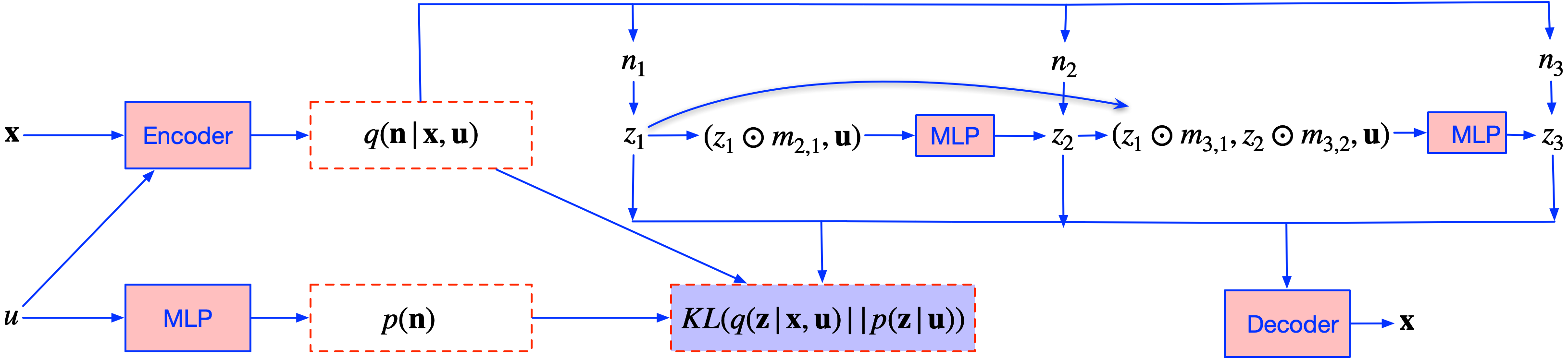
In this section, we translate our theoretical findings into a novel method for learning latent causal models. Our primary focus is on learning additive noise models, as extending the method to latent post-nonlinear models is straightforward, simply involving the utilization of invertible nonlinear mappings as mentioned in Discussion for Corollary 3.1. Following previous works in Liu et al. (2022, 2023), due to permutation indeterminacy in latent space, we can naturally enforce a causal order without specific semantic information. With guarantee from Theorem 2.1, each variable can be imposed to learn the corresponding latent variables in the correct causal order. As a result, we formulate prior model as follows:
| (6) |
where we focus on latent Gaussian noise variables, considering the re-parametric trick, and we introduce additional vectors , by enforcing sparsity on and the component-wise product , to attentively learn latent causal graph structure. In our implementation, we simply impose norm, other methods may also be flexible, e.g., considering sparsity priors (Carvalho et al., 2009; Liu et al., 2019).
We employ the following variational posterior to approximate the true intractable posterior of :
| (7) |
where the variational posterior shares the same parameter to contrast with both the prior and the variational posterior, maintaining the same latent causal graph structure. As a result, we can arrive at a simple objective:
| (8) |
where denotes the KL divergence, denotes a hyperparameters to control the sparsity of latent causal structure. Implementation details can be found in Appendix G.
5 Experiments
Synthetic Data
We first conduct experiments on synthetic data, generated by the following process: we divide latent noise variables into segments, where each segment corresponds to one value of as the segment label. Within each segment, the location and scale parameters are respectively sampled from uniform priors. After generating latent noise variables, we generate latent causal variables, and finally obtain the observed data samples by an invertible nonlinear mapping on the causal variables. More details can be found in Appendix F.
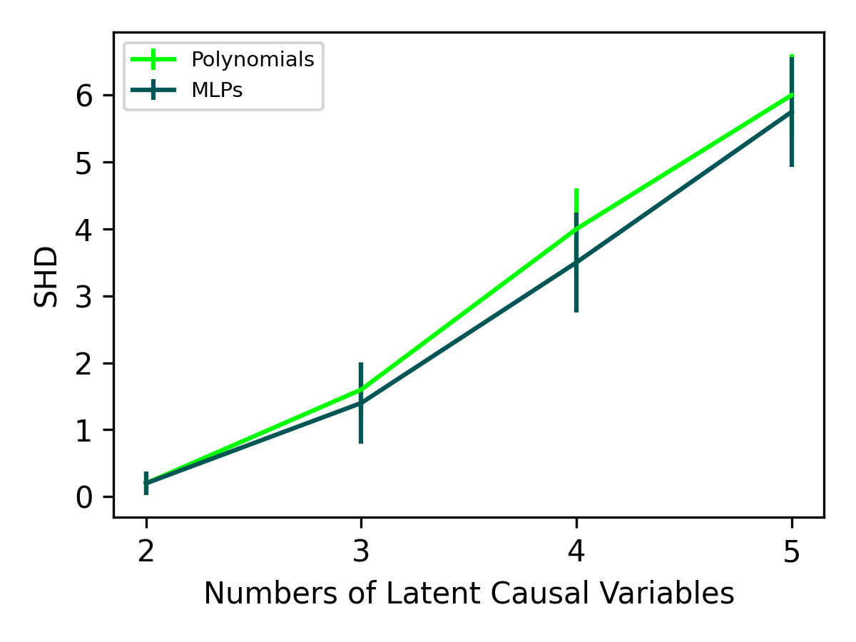
We evaluate our proposed method (MLPs), implemented by MLPs to model the causal relations among latent causal variables, against established models: vanilla VAE (Kingma & Welling, 2013), -VAE (Higgins et al., 2017), identifiable VAE (iVAE) (Khemakhem et al., 2020), and latent polynomial models (Polynomials) (Liu et al., 2023). Notably, the iVAE demonstrates the capability to identify true independent noise variables, subject to certain conditions, with permutation and scaling. Polynomials, while sharing similar assumptions with our proposed method, are prone to certain limitations. Specifically, they may suffer from numerical instability and face challenges due to the exponential growth in the number of terms. While the -VAE is popular in disentanglement tasks due to its emphasis on independence among recovered variables, it lacks robust theoretical backing. Our evaluation focuses on two metrics: the Mean of the Pearson Correlation Coefficient (MPC) to assess performance, and the Structural Hamming Distance (SHD) to gauge the accuracy of the latent causal graphs recovered by our method.
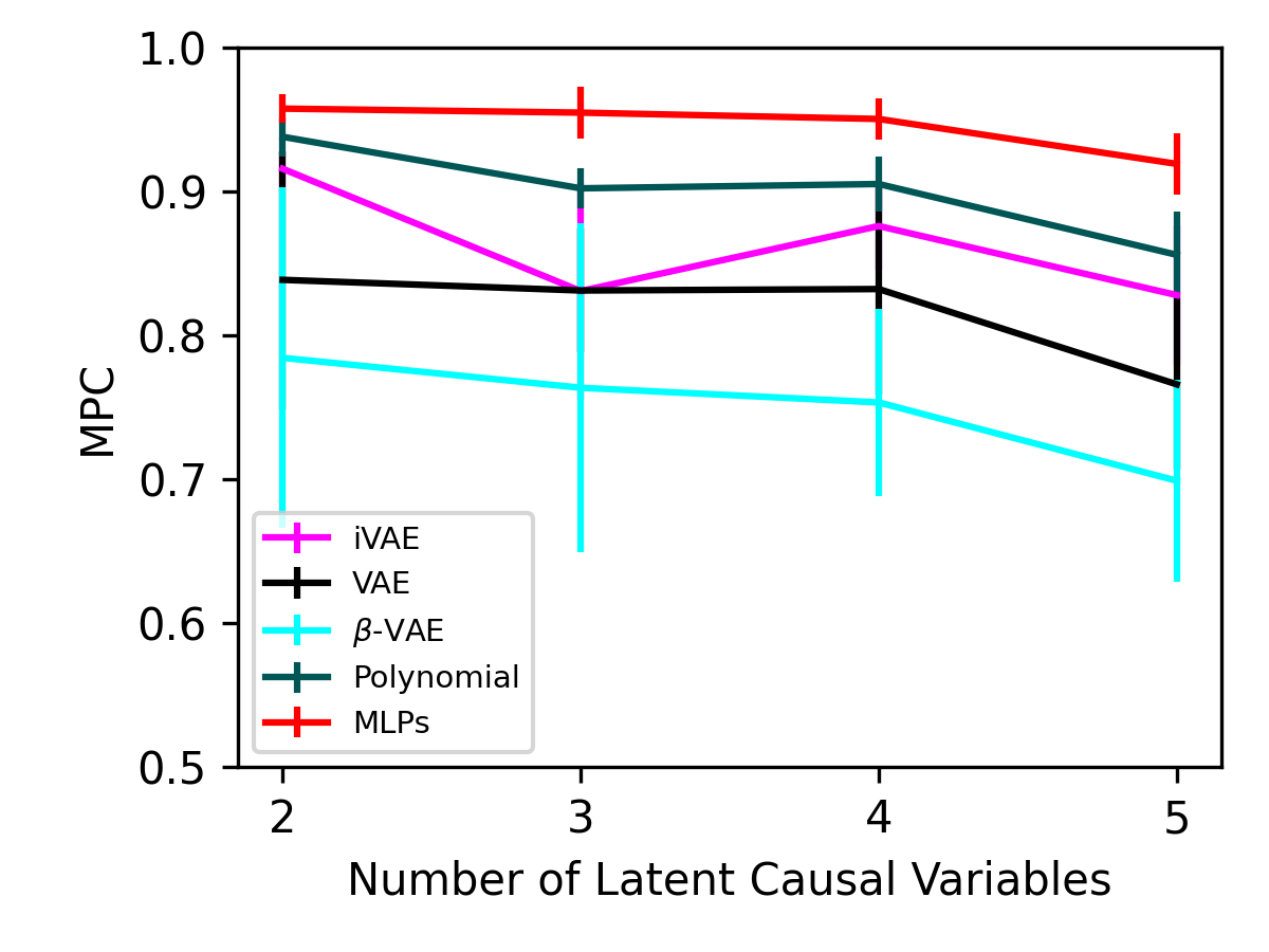
MPC
SHD
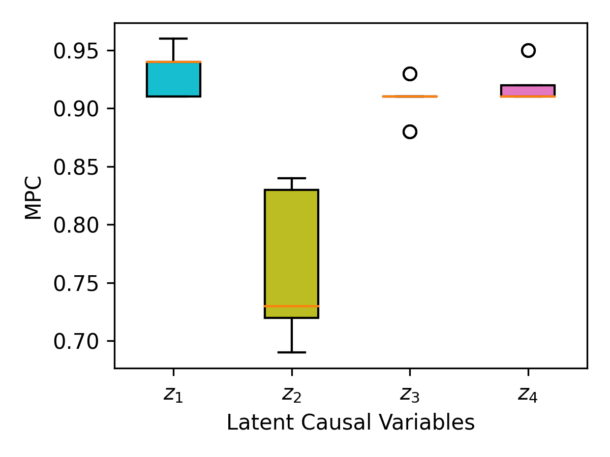
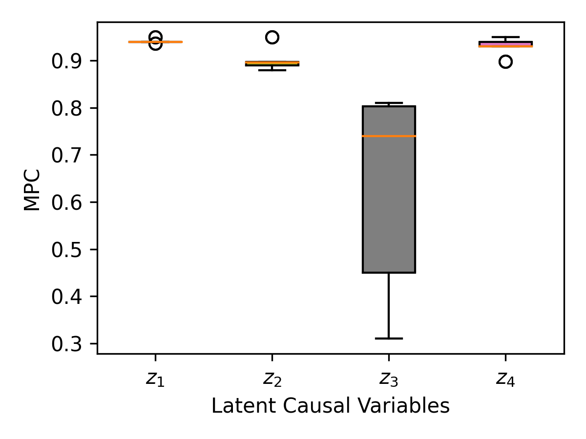
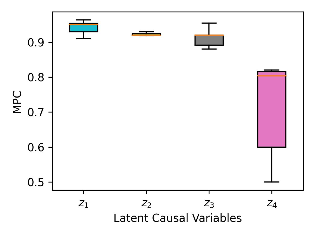
Figure 1 illustrates the comparative performances of various methods across different models. Based on MPC, the proposed method demonstrates satisfactory results, thereby supporting our identifiability claims. Additionally, Figure 2 presents how the proposed method performs when condition (iv) is not met. It is evident that condition (iv) is a sufficient and necessary condition characterizing the types of distribution shifts for identifiability in the context of latent additive noise models. These empirical findings align with the partial identifiability conclusions discussed in Corollary 2.5.
Post-Nonlinear Models
In the above experiments, we obtain the observed data samples as derived from a random invertible nonlinear mapping applied to the latent causal variables. The nonlinear mapping can be conceptualized as a combination of an invertible transformation and the specific invertible mapping, , as mentioned in Discussion for Corollary 3.1. From this perspective, the results depicted in Figures 1 and 2 also demonstrate the effectiveness of the proposed method in recovering the variables in latent post-nonlinear models Eq. (5), as well as the associated latent causal structures. Consequently, these results also serve to corroborate the assertions made in Corollary 3.1 and Corollary 3.3, particularly given that are defined as invertible mappings.
Image Data
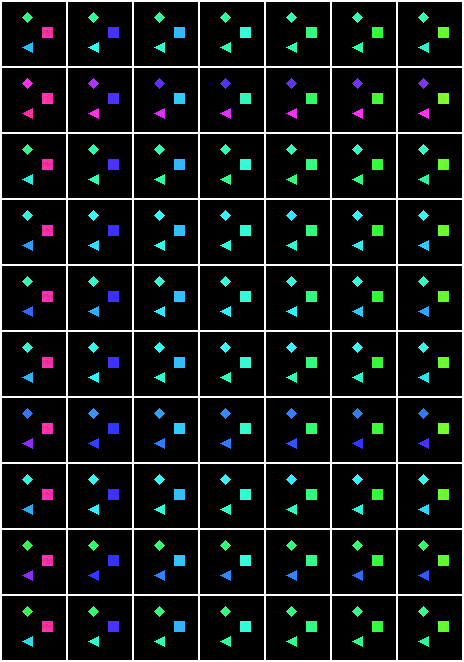
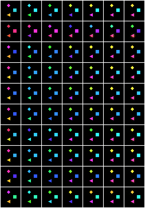
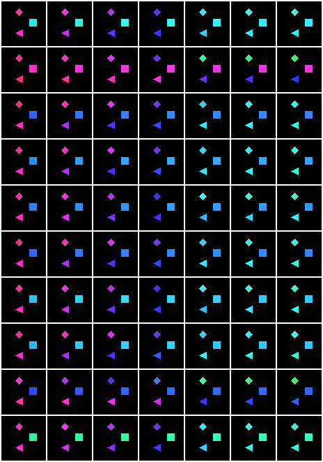
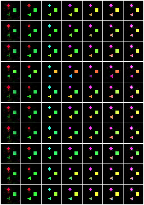
We further validate our proposed identifiability results and methodology using images from the chemistry dataset introduced by Ke et al. (2021). This dataset is representative of chemical reactions where the state of one element can influence the state of another. The images feature multiple objects with fixed positions, but their colors, representing different states, change according to a predefined causal graph. To align with our theoretical framework, we employ a nonlinear model with additive Gaussian noise for generating latent variables that correspond to the colors of these objects. The established latent causal graph within this context indicates that the ‘diamond’ object (denoted as ) influences the ‘triangle’ (), which in turn affects the ‘square’ (). Figure 3 provides a visual representation of these observational images, illustrating the causal relationships in a tangible format.
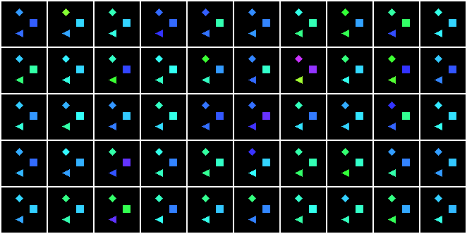
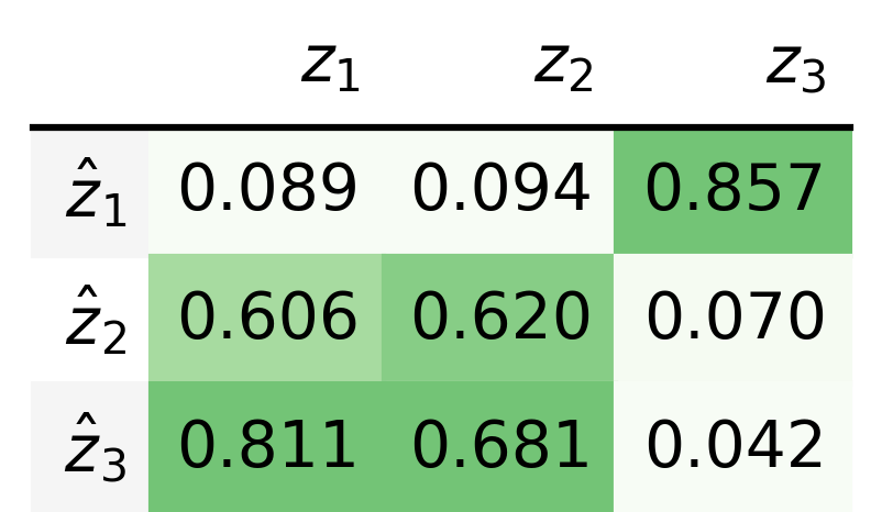
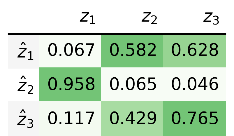
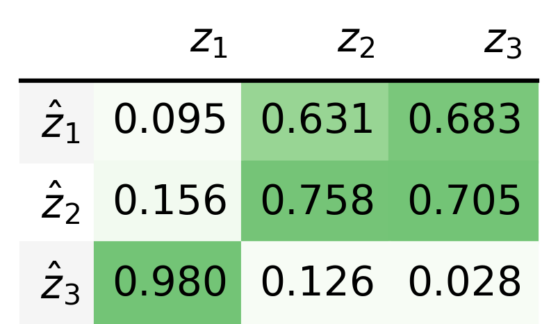
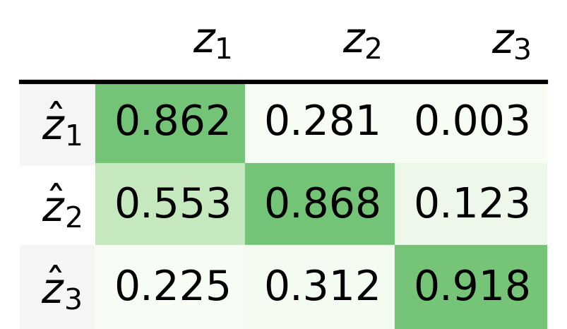
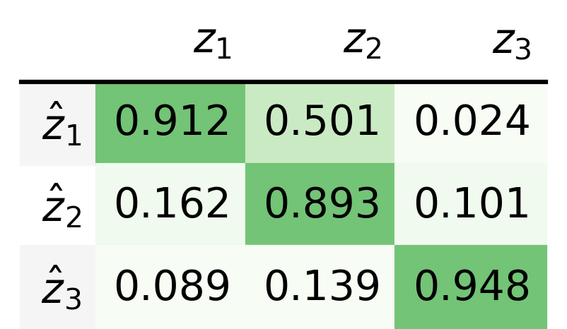
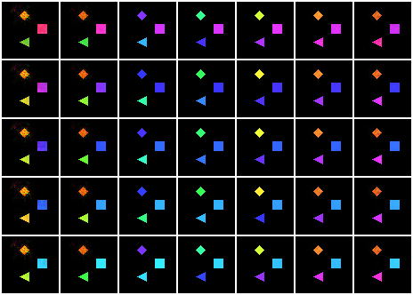
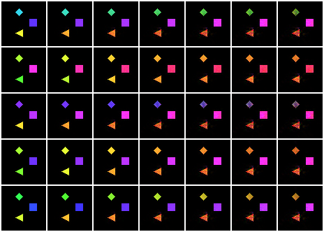
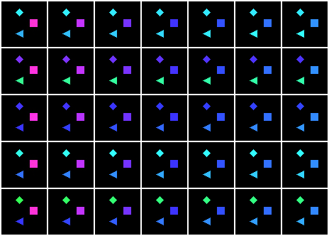
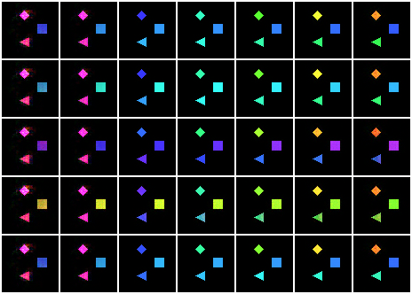
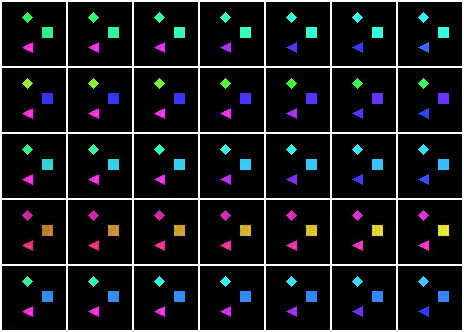
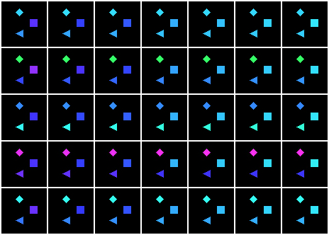
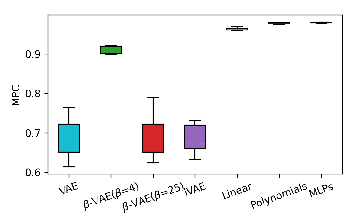
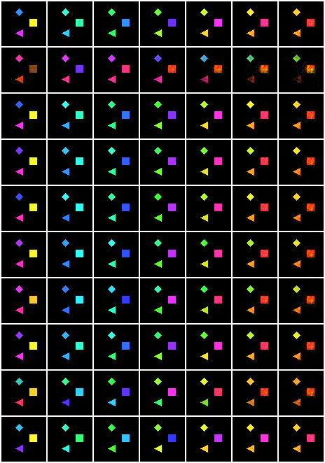
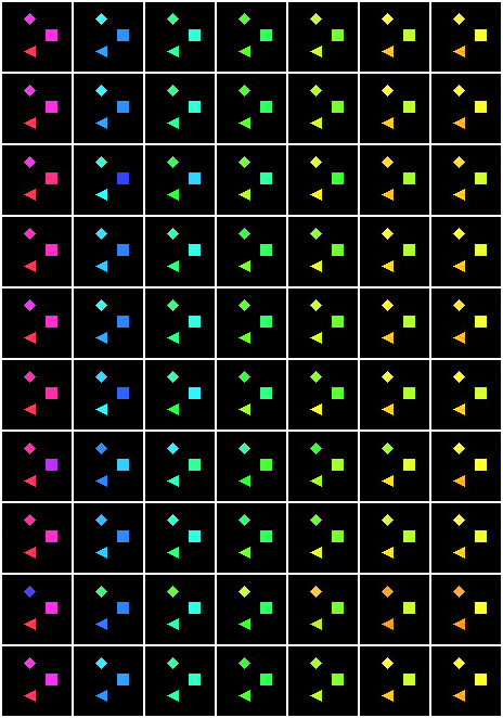
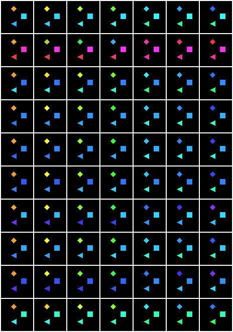
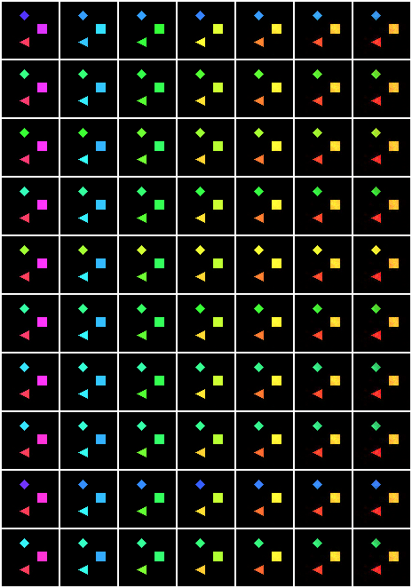
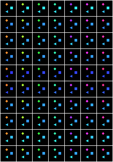
Figure 4 presents MPC outcomes as derived from various methods. Among these, the proposed method demonstrates superior performance. In addition, both the proposed method (MLPs) and Polynomials can accurately learn the causal graph, as corroborated by the intervention outcomes depicted in Figures 5-6. However, Polynomial encounters issues such as numerical instability and exponential growth in terms, which compromises its performance in MPC, as seen in Figure 4. This superiority of MLPs is further evidenced in the intervention results on , as depicted in Figures 5-6. Specifically, the visual influences on displayed in Figure 6 less than those observed in Figure 5. Owing to space constraints, additional traversal results concerning the learned latent variables from other methodologies are detailed in Appendix H. Note that for these methods, lacking a guarantee of identifiability, our observations indicate that traversing any learned variable results in a change in color across all objects.
fMRI Data
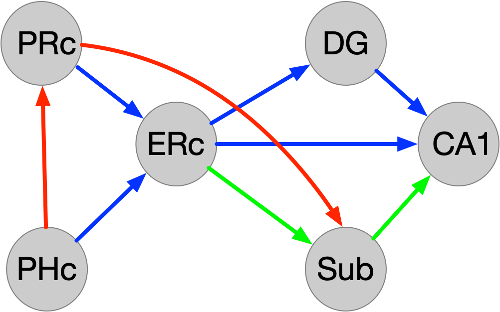
Building on the works in Liu et al. (2022, 2023), we extended the application of the proposed method to the fMRI hippocampus dataset (Laumann & Poldrack, 2015). This dataset comprises signals from six distinct brain regions: perirhinal cortex (PRC), parahippocampal cortex (PHC), entorhinal cortex (ERC), subiculum (Sub), CA1, and CA3/Dentate Gyrus (DG). These signals, recorded during resting states, span 84 consecutive days from a single individual. Each day’s data contributes to an 84-dimensional vector, denoted as . Our focus centers on uncovering latent causal variables, and thus we consider these six brain signals as such. For analysis, these signals undergo a random nonlinear mapping to transform them into observable data. Various methods are then employed on this transformed data, aiming to recover the underlying latent causal variables.
Linear
Polynomials
MLPs
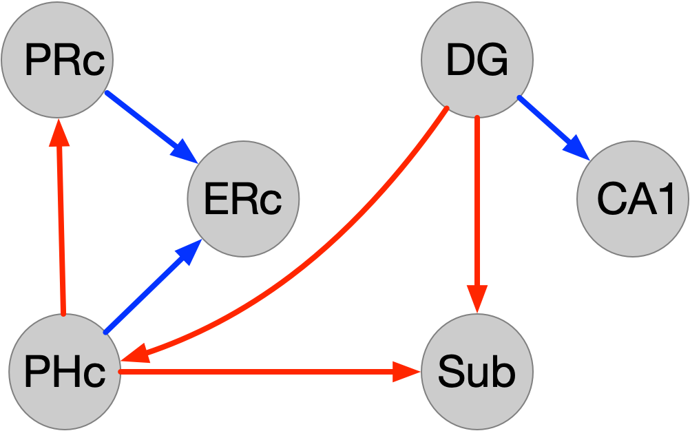
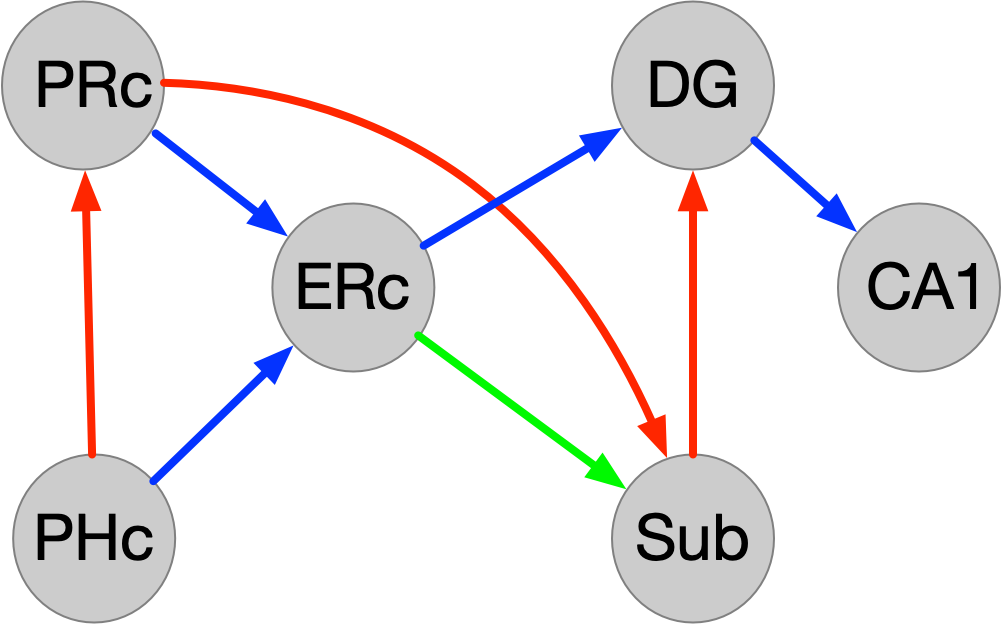
Figure 7 presents the comparative results yielded by the proposed method alongside various other methods. Notably, the VAE, -VAE, and iVAE models presume the independence of latent variables, rendering them incapable of discerning the underlying latent causal structure. Similar to the findings of Liu et al. (2022), we noted that promoting independence (e.g., setting ) actually deteriorates the model performance criterion (MPC), whereas loosening this constraint (albeit still within its inherent assumption of independence, such as setting ) enhances performance. This phenomenon likely stems from the non-independence of latent variables conditioned on the time index within this specific dataset. Conversely, other methods, including latent linear models, latent polynomials, and latent MLPs, are able to accurately recover the latent causal structure with guarantees. Among these, the MLP models outperform the others in terms of MPC. In the study by Liu et al. (2023), it is noted that linear relationships among the examined signals tend to be more prominent than nonlinear ones. This observation might lead to the presumption that linear models would be effective. However, this is not necessarily the case, as these models can still yield suboptimal outcomes. In contrast, MLPs demonstrate superior performance in term of MPC, particularly when compared to polynomial models, which are prone to instability and exponential growth issues. The effectiveness of MLPs is further underscored by their impressive average MPC score of 0.981. This advantage is visually represented in Figure 8, which illustrates the enhanced capability of MLPs in uncovering latent causal structures.
6 Conclusion
This study offers a pivotal contribution by establishing a sufficient and necessary condition that precisely characterizes the types of distribution shifts crucial for the identifiability of latent additive noise models. Additionally, we delve into scenarios where only a subset of distribution shifts fulfills this condition, presenting insights into partial identifiability in such contexts. Building upon these foundational principles, the research extends its applicability to latent post-nonlinear causal models, broadening the scope of its theoretical implications. We translat these theoretical concepts into a practical method, extensive empirical testing was conducted on a diverse array of datasets, including both synthetic and real-world examples. Exploring the connection between distribution shifts and identifying latent non-parametric models presents a potentially rich area.
7 Impact Statement
This paper presents work whose goal is to advance the field of Machine Learning. There are many potential societal consequences of our work, none which we feel must be specifically highlighted here.
References
- Adams et al. (2021) Adams, J., Hansen, N., and Zhang, K. Identification of partially observed linear causal models: Graphical conditions for the non-gaussian and heterogeneous cases. In NeurIPS, 2021.
- Ahuja et al. (2023) Ahuja, K., Mahajan, D., Wang, Y., and Bengio, Y. Interventional causal representation learning. In International Conference on Machine Learning, pp. 372–407. PMLR, 2023.
- Anandkumar et al. (2013) Anandkumar, A., Hsu, D., Javanmard, A., and Kakade, S. Learning linear bayesian networks with latent variables. In ICML, pp. 249–257, 2013.
- Brehmer et al. (2022) Brehmer, J., De Haan, P., Lippe, P., and Cohen, T. Weakly supervised causal representation learning. arXiv preprint arXiv:2203.16437, 2022.
- Buchholz et al. (2023) Buchholz, S., Rajendran, G., Rosenfeld, E., Aragam, B., Schölkopf, B., and Ravikumar, P. Learning linear causal representations from interventions under general nonlinear mixing. arXiv preprint arXiv:2306.02235, 2023.
- Cai et al. (2019) Cai, R., Xie, F., Glymour, C., Hao, Z., and Zhang, K. Triad constraints for learning causal structure of latent variables. In NeurIPS, 2019.
- Carvalho et al. (2009) Carvalho, C. M., Polson, N. G., and Scott, J. G. Handling sparsity via the horseshoe. In Artificial intelligence and statistics, pp. 73–80. PMLR, 2009.
- Chandrasekaran et al. (2021) Chandrasekaran, S. N., Ceulemans, H., Boyd, J. D., and Carpenter, A. E. Image-based profiling for drug discovery: due for a machine-learning upgrade? Nature Reviews Drug Discovery, 20(2):145–159, 2021.
- Forbes & Krueger (2019) Forbes, M. K. and Krueger, R. F. The great recession and mental health in the united states. Clinical Psychological Science, 7(5):900–913, 2019.
- Frot et al. (2019) Frot, B., Nandy, P., and Maathuis, M. H. Robust causal structure learning with some hidden variables. Journal of the Royal Statistical Society: Series B (Statistical Methodology), 81(3):459–487, 2019.
- Ghassami et al. (2018) Ghassami, A., Kiyavash, N., Huang, B., and Zhang, K. Multi-domain causal structure learning in linear systems. Advances in neural information processing systems, 31, 2018.
- Gibbs & Candes (2021) Gibbs, I. and Candes, E. Adaptive conformal inference under distribution shift. Advances in Neural Information Processing Systems, 34:1660–1672, 2021.
- Higgins et al. (2017) Higgins, I., Matthey, L., Pal, A., Burgess, C. P., Glorot, X., Botvinick, M., Mohamed, S., and Lerchner, A. beta-vae: Learning basic visual concepts with a constrained variational framework. In ICLR, 2017.
- Hoyer et al. (2008) Hoyer, P. O., Janzing, D., Mooij, J. M., Peters, J., Schölkopf, B., et al. Nonlinear causal discovery with additive noise models. In NeurIPS, volume 21, pp. 689–696. Citeseer, 2008.
- Huang* et al. (2020) Huang*, B., Zhang*, K., Zhang, J., Ramsey, J., Sanchez-Romero, R., Glymour, C., and Schölkopf, B. Causal discovery from heterogeneous/nonstationary data. JMLR, 21(89), 2020.
- Huang et al. (2022) Huang, B., Low, C. J. H., Xie, F., Glymour, C., and Zhang, K. Latent hierarchical causal structure discovery with rank constraints. Advances in Neural Information Processing Systems, 35:5549–5561, 2022.
- Hyvarinen & Morioka (2016) Hyvarinen, A. and Morioka, H. Unsupervised feature extraction by time-contrastive learning and nonlinear ica. Advances in neural information processing systems, 29, 2016.
- Hyvarinen et al. (2019) Hyvarinen, A., Sasaki, H., and Turner, R. Nonlinear ica using auxiliary variables and generalized contrastive learning. In The 22nd International Conference on Artificial Intelligence and Statistics, pp. 859–868. PMLR, 2019.
- Ke et al. (2021) Ke, N. R., Didolkar, A., Mittal, S., Goyal, A., Lajoie, G., Bauer, S., Rezende, D., Bengio, Y., Mozer, M., and Pal, C. Systematic evaluation of causal discovery in visual model based reinforcement learning. arXiv preprint arXiv:2107.00848, 2021.
- Khemakhem et al. (2020) Khemakhem, I., Kingma, D., Monti, R., and Hyvarinen, A. Variational autoencoders and nonlinear ica: A unifying framework. In AISTAS, pp. 2207–2217. PMLR, 2020.
- Kingma & Welling (2013) Kingma, D. P. and Welling, M. Auto-encoding variational bayes. arXiv preprint arXiv:1312.6114, 2013.
- Kong et al. (2022) Kong, L., Xie, S., Yao, W., Zheng, Y., Chen, G., Stojanov, P., Akinwande, V., and Zhang, K. Partial disentanglement for domain adaptation. In International Conference on Machine Learning, pp. 11455–11472. PMLR, 2022.
- Lachapelle et al. (2021) Lachapelle, S., López, P. R., Sharma, Y., Everett, K., Priol, R. L., Lacoste, A., and Lacoste-Julien, S. Disentanglement via mechanism sparsity regularization: A new principle for nonlinear ica. arXiv preprint arXiv:2107.10098, 2021.
- Laumann & Poldrack (2015) Laumann, T. O. and Poldrack, R. A., 2015. URL https://openfmri.org/dataset/ds000031/.
- Lippe et al. (2022a) Lippe, P., Magliacane, S., Löwe, S., Asano, Y. M., Cohen, T., and Gavves, E. Causal representation learning for instantaneous and temporal effects in interactive systems. In The Eleventh International Conference on Learning Representations, 2022a.
- Lippe et al. (2022b) Lippe, P., Magliacane, S., Löwe, S., Asano, Y. M., Cohen, T., and Gavves, S. Citris: Causal identifiability from temporal intervened sequences. In International Conference on Machine Learning, pp. 13557–13603. PMLR, 2022b.
- Liu et al. (2019) Liu, Y., Dong, W., Zhang, L., Gong, D., and Shi, Q. Variational bayesian dropout with a hierarchical prior. In CVPR, 2019.
- Liu et al. (2022) Liu, Y., Zhang, Z., Gong, D., Gong, M., Huang, B., Hengel, A. v. d., Zhang, K., and Shi, J. Q. Identifying weight-variant latent causal models. arXiv preprint arXiv:2208.14153, 2022.
- Liu et al. (2023) Liu, Y., Zhang, Z., Gong, D., Gong, M., Huang, B., Hengel, A. v. d., Zhang, K., and Shi, J. Q. Identifiable latent polynomial causal models through the lens of change. arXiv preprint arXiv:2310.15580, 2023.
- Pearl (2000) Pearl, J. Causality: Models, Reasoning, and Inference. Cambridge University Press, Cambridge, 2000.
- Peters et al. (2014) Peters, J., Mooij, J. M., Janzing, D., and Schölkopf, B. Causal discovery with continuous additive noise models. JMLR, 15(58):2009–2053, 2014.
- Peters et al. (2017) Peters, J., Janzing, D., and Schlkopf, B. Elements of Causal Inference: Foundations and Learning Algorithms. The MIT Press, 2017.
- Pinsky et al. (2020) Pinsky, M. L., Selden, R. L., and Kitchel, Z. J. Climate-driven shifts in marine species ranges: Scaling from organisms to communities. Annual review of marine science, 12:153–179, 2020.
- Schölkopf et al. (2021) Schölkopf, B., Locatello, F., Bauer, S., Ke, N. R., Kalchbrenner, N., Goyal, A., and Bengio, Y. Toward causal representation learning. Proceedings of the IEEE, 109(5):612–634, 2021.
- Seigal et al. (2022) Seigal, A., Squires, C., and Uhler, C. Linear causal disentanglement via interventions. arXiv preprint arXiv:2211.16467, 2022.
- Shimizu et al. (2009) Shimizu, S., Hoyer, P. O., and Hyvärinen, A. Estimation of linear non-gaussian acyclic models for latent factors. Neurocomputing, 72(7-9):2024–2027, 2009.
- Silva et al. (2006) Silva, R., Scheines, R., Glymour, C., Spirtes, P., and Chickering, D. M. Learning the structure of linear latent variable models. JMLR, 7(2), 2006.
- Sorrenson et al. (2020) Sorrenson, P., Rother, C., and Köthe, U. Disentanglement by nonlinear ica with general incompressible-flow networks (gin). arXiv preprint arXiv:2001.04872, 2020.
- Spirtes et al. (2001) Spirtes, P., Glymour, C., and Scheines, R. Causation, Prediction, and Search. MIT Press, Cambridge, MA, 2nd edition, 2001.
- Varici et al. (2023) Varici, B., Acarturk, E., Shanmugam, K., Kumar, A., and Tajer, A. Score-based causal representation learning with interventions. arXiv preprint arXiv:2301.08230, 2023.
- Von Kügelgen et al. (2021) Von Kügelgen, J., Sharma, Y., Gresele, L., Brendel, W., Schölkopf, B., Besserve, M., and Locatello, F. Self-supervised learning with data augmentations provably isolates content from style. In Advances in neural information processing systems, 2021.
- Wang et al. (2022) Wang, X., Saxon, M., Li, J., Zhang, H., Zhang, K., and Wang, W. Y. Causal balancing for domain generalization. arXiv preprint arXiv:2206.05263, 2022.
- Xie et al. (2020) Xie, F., Cai, R., Huang, B., Glymour, C., Hao, Z., and Zhang, K. Generalized independent noise condition for estimating latent variable causal graphs. In NeurIPS, 2020.
- Xie et al. (2022a) Xie, F., Huang, B., Chen, Z., He, Y., Geng, Z., and Zhang, K. Identification of linear non-gaussian latent hierarchical structure. In International Conference on Machine Learning, pp. 24370–24387. PMLR, 2022a.
- Xie et al. (2022b) Xie, S., Kong, L., Gong, M., and Zhang, K. Multi-domain image generation and translation with identifiability guarantees. In The Eleventh International Conference on Learning Representations, 2022b.
- Yao et al. (2021) Yao, W., Sun, Y., Ho, A., Sun, C., and Zhang, K. Learning temporally causal latent processes from general temporal data. arXiv preprint arXiv:2110.05428, 2021.
- Yao et al. (2022) Yao, W., Chen, G., and Zhang, K. Learning latent causal dynamics. arXiv preprint arXiv:2202.04828, 2022.
- Zhang et al. (2023) Zhang, J., Squires, C., Greenewald, K., Srivastava, A., Shanmugam, K., and Uhler, C. Identifiability guarantees for causal disentanglement from soft interventions. arXiv preprint arXiv:2307.06250, 2023.
- Zhang & Hyvärinen (2009) Zhang, K. and Hyvärinen, A. On the identifiability of the post-nonlinear causal model. In Proceedings of the 25th Conference on Uncertainty in Artificial Intelligence, Montreal, Canada, 2009.
Appendix A Related Work
Given the challenges associated with identifiability in causal representation learning, numerous existing works tackle this issue by introducing specific assumptions. We categorize these related works into three primary parts based on the nature of these assumptions.
Special graph structure Some progress in achieving identifiability centers around the imposition of specific graphical structure constraints (Silva et al., 2006; Shimizu et al., 2009; Anandkumar et al., 2013; Frot et al., 2019; Cai et al., 2019; Xie et al., 2020, 2022a; Lachapelle et al., 2021). Essentially, these graph structure assumptions reduce the space of possible latent causal representations or structures, by imposing specific rules for how variables are connected in the graph. One popular special graph structure assumption is the presence of two pure children nodes for each causal variable (Xie et al., 2020, 2022a; Huang et al., 2022). Very recently, the work in (Adams et al., 2021) provides a viewpoint of sparsity to understand previous various graph structure constraints, i.e., various previous graph structure constraints generally seek sparser graphs. However, any complex causal graphs may appear in real-world scenarios, beyond the pure sparsity assumption. In contrast, our approach adopts a model-based representation for latent variables, allowing arbitrary underlying graph structures.
Temporal Information The temporal constraint that the effect cannot precede the cause has been applied in causal representation learning (Yao et al., 2021; Lippe et al., 2022b; Yao et al., 2022; Lippe et al., 2022a). The success of utilizing temporal information to identify causal representations can be attributed to its innate ability to establish causal direction through time delay. By tracking the sequence of events over time, we gain the capacity to infer latent causal variables. In contrast to these existing approaches, our focus lies on discovering instantaneous causal relations among latent variables.
Distribution shifts Exploring distribution shifts for identifying causal representations has been significantly developed recently (Von Kügelgen et al., 2021; Liu et al., 2022; Brehmer et al., 2022; Ahuja et al., 2023; Seigal et al., 2022; Buchholz et al., 2023; Varici et al., 2023). The key question is how to model the types of distribution shifts contributing to identifiability. The majority of works focus on using hard interventions to capture the types of distribution shifts, with some specifically considering single-node hard interventions (Ahuja et al., 2023; Seigal et al., 2022; Buchholz et al., 2023; Varici et al., 2023). However, hard interventions may only capture the specific types of distribution shifts. In contrast, soft interventions offer the potential to model a wider array of distribution shifts (Liu et al., 2022, 2023). Unfortunately, the work in Liu et al. (2022) assumes the underlying causal relations among latent causal variables to be linear models, the work in Liu et al. (2023) explores distribution shifts in the context of latent polynomial models, which are susceptible to issues such as numerical instability and exponential growth in terms. In this work, we explores distribution shifts in general latent additive noise models, and extend it to more powerful latent post-nonlinear models. This work also differs from the recent study by Zhang et al. (2023) in several ways. While the latter assumes the mixing function from latent causal variables to observational data is a full row rank polynomial—a constraint that may be limiting in real-world applications—we impose no such restriction. Furthermore, Zhang et al. (2023) requires single-node interventions, where an intervention on each latent node is available. This requirement may be particularly limiting, especially when considering the distribution shifts resulting from self-initiated behaviors within a causal system. In contrast, our approach does not necessitate single-node interventions.
Appendix B The Proof of Theorem 2.1
For convenience, we first introduce the following lemmas.
Lemma B.1.
Denote the mapping from to as . This mapping, , is invertible, and its Jacobian determinant is equal to 1, i.e., .
The proof unfolds straightforwardly as follows: Acknowledging that depends contingent on its parents and , as delineated in Eq. 2, allows us to iteratively represent in terms of the latent noise variables associated with its parents alongside . More explicitly, without loss of the generality, by assuming the true causal order to be , we can deduce:
| (9) | |||
where . Furthermore, according to the additive noise models and DAG constraints, it can be shown that the Jacobi determinant of equals 1, and thus the mapping is invertible.
Lemma B.2.
The mapping from to , e.g., , is invertible, and the Jacobi determinant , and thus , which do not depend on .
The proof can be succinctly articulated as follows: Lemma B.1 confirms the invertibility of the mapping from to . When this is coupled with Assumption (ii), which posits the invertibility of , it follows that the transformation from to is also invertible. Furthermore, the condition , as established by Lemma B.1, leads us to:
and,
Lemma B.3.
The proof can be constructed as follows: Given that the partial derivative of the mapping corresponds to the partial derivative of , and leveraging Assumption (iv) in conjunction with the chain rule, we are able to deduce the desired result.
The proof of Theorem 2.1 unfolds in three distinct steps. Initially, Step I establishes that the identifiability criterion from (Sorrenson et al., 2020) is applicable in our context. Specifically, it confirms that the latent noise variables are identifiable, subject only to component-wise scaling and permutation, expressed as . Building on this, Step II demonstrates a linkage between the recovered latent causal variables and the true , formulated as . Finally, Step III utilizes Lemma B.3 to illustrate that the transformation , introduced in Step II, essentially simplifies to a combination of permutation and scaling, articulated as .
Step I: Suppose we have two sets of parameters and corresponding to the same conditional probabilities, i.e., for all pairs , where denote the sufficient statistic of latent noise variables . Due to the assumption (i), the assumption (ii), and the fact that is invertible (e.g., Lemma B.1), by expanding the conditional probabilities (More details can be found in Step I for proof of Theorem 1 in (Khemakhem et al., 2020)), we have:
| (10) |
Using the exponential family as defined in Eq. (1), we have:
| (11) | |||
| (12) |
By using Lemma B.2, Eqs. (11)-(12) can be reduced to:
| (13) |
Then by expanding the above at points and , then using Eq. 13 at point subtract Eq. 13 at point , we find:
| (14) |
Here . By assumption (iii), and combining the expressions into a single matrix equation, we can write this in terms of from assumption (iii),
| (15) |
Since is invertible, we can multiply this expression by its inverse from the left to get:
| (16) |
Where . According to lemma 3 in (Khemakhem et al., 2020) that there exist distinct values to such that the derivative are linearly independent, and the fact that each component of is univariate, we can show that is invertible.
Since we assume the noise to be two-parameter exponential family members, Eq. 16 can be re-expressed as:
| (17) |
Then, we re-express in term of , e.g., where is a nonlinear mapping. As a result, we have from Eq. 17 that: (a) can be linear combination of and , and (b) can also be linear combination of and . This implies the contradiction that both and its nonlinear transformation can be expressed by linear combination of and . This contradiction leads to that can be reduced to permutation matrix (See APPENDIX C in (Sorrenson et al., 2020) for more details):
| (18) |
where denote the permutation matrix with scaling, denote a constant vector. Note that this result holds for not only Gaussian, but also inverse Gaussian, Beta, Gamma, and Inverse Gamma (See Table 1 in (Sorrenson et al., 2020)).
Step II:By Lemma B.1, we can denote and by:
| (19) | |||
| (20) |
where is defined in B.1. Replacing and in Eq. 18 by Eq. 19 and Eq. 20, respectively, we have:
| (21) |
where (as well as ) are invertible supported by Lemma B.1. We can rewrite Eq. 21 as:
| (22) |
Denote the composition by , we have:
| (23) |
| (24) |
By differentiating Eq. 24 with respect to
| (25) |
Without loss of generality, let us consider the correct causal order so that and are lower triangular matrices whose the diagonal are 1, and is a diagonal matrix with elements .
Elements above the diagonal of matrix
Since is a lower triangular matrix, and is a diagonal matrix, must be a lower triangular matrix.
Then by expanding the left side of Eq. 25, we have:
| (26) |
by expanding the right side of Eq. 25, we have:
| (27) |
The diagonal of matrix
Elements below the diagonal of matrix
As a result, the matrix in Eq. 25 equals to the permutation matrix , which implies that the transformation Eq. 23 reduces to a permutation transformation,
| (28) |
In the preceding proof, it becomes evident that assumption (iv) (or Lemma B.3) is sufficient to constrain the elements below the diagonal of the matrix to zero. Therefore, our primary objective now shifts to the verification of what happens when assumption (iv) is not met – specifically, whether the claim that the elements below the diagonal of are zero still holds or not. We will proof that in next section.
Appendix C The Proof of Theorem 2.5
Since the proof process in Steps I and II in B do not depend on the assumption (iv), the results in both Eq. 26 and Eq. 27 hold. Then consider the following two cases.
- •
-
•
In cases where assumption (iv) does not hold for , such as when we compare Eq. (26) with Eq. (27), we are unable to conclude that the -th row of the Jacobian matrix contains only one element. For example, consider , and by comparing Eq. (26) with Eq. (27), we can derive the following equation: . In this case, if assumption (iv) does not hold for , i.e., there does not exist a point or value for that and , then when holds true, we can match the true marginal data distribution . This implies that can have a non-zero value. Consequently, can be represented as a combination of and , resulting in unidentifiability. Note that this unidentifiability result also show that the necessity of condition (iv) for achieving complete identifiability, by the contrapositive, i.e., if is identifiable, then condition (iv) is satisfied.
Appendix D The Proof of Corollary 3.1
The proof can be done from the following: since in Theorem 2.1, the only constraint imposed on the function is that the function is injective, as mentioned in condition (ii). Consequently, we can create a new function by composing with function , in which each component is defined by the function . Since in invertible as defined in Eq. 5, remains injective. As a result, we can utilize the proof from Appendix B to obtain that can be identified up to permutation and scaling, i.e., Eq. (28) holds. Finally, given the existence of a component-wise invertible nonlinear mapping between and as defined in Eq. 5, i.e.,
| (29) |
we can also obtain estimated by enforcing a component-wise invertible nonlinear mapping on the recovered
| (30) |
Replacing and in Eq. (28) by Eq. (29) and Eq. (30), respectively, we have
| (31) |
As a result, we conclude the proof.
Appendix E The Proof of Corollary 3.3
Again, since in Theorem 2.1, the only constraint imposed on the function is that the function is injective, as mentioned in condition (ii). Consequently, we can create a new function by composing with function , in which each component is defined by the function . Since is invertible as defined in Eq. 5, remains injective. Given the above, the results in both Eq. 26 and Eq. 27 hold. Then consider the following two cases.
-
•
In cases where represents a root node or assumption (iv) holds true for , using the proof in Appendix E we can obtain that . Then, given the existence of a component-wise invertible nonlinear mapping between and as defined in Eq. 5, we can proof that there is a invertible mapping between the recovered and the true .
- •
Appendix F Data Details
Synthetic Data
In our experimental results using synthetic data, we utilize 50 segments, with each segment containing a sample size of 1000. Furthermore, we explore latent causal or noise variables with dimensions of 2, 3, 4, and 5, respectively. Specifically, our analysis centers around the following structural causal model:
| (32) | ||||
| (33) | ||||
| (34) | ||||
| (35) | ||||
| (36) | ||||
| (37) |
In this context, both and for Gaussian noise are drawn from uniform distributions within the ranges of and , respectively. The values of are sampled from a uniform distribution spanning
Synthetic Data for Partial Identifiability
Image Data
In our experimental results using image data, we consider the following latent structural causal model:
| (40) | ||||
| (41) | ||||
| (42) | ||||
| (43) |
where both and for Gaussian noise are drawn from uniform distributions within the ranges of and , respectively. The values of are sampled from a uniform distribution spanning .
Appendix G Implementation Framework
Figure 9 illustrates our proposed method for learning latent nonlinear models with additive Gaussian noise. In our experiments with synthetic and fMRI data, we implemented the encoder, decoder, and MLPs using three-layer fully connected networks, complemented by Leaky-ReLU activation functions. For optimization, the Adam optimizer was employed with a learning rate of 0.001. In the case of image data experiments, the prior model also utilized a three-layer fully connected network with Leaky-ReLU activation functions. The encoder and decoder designs were adopted from Liu et al. (2023) and are detailed in Table 1 and Table 2, respectively.
| Input |
|---|
| Leaky-ReLU(Conv2d(3, 32, 4, stride=2, padding=1)) |
| Leaky-ReLU(Conv2d(32, 32, 4, stride=2, padding=1)) |
| Leaky-ReLU(Conv2d(32, 32, 4, stride=2, padding=1)) |
| Leaky-ReLU(Conv2d(32, 32, 4, stride=2, padding=1)) |
| Leaky-ReLU(Linear(32324 size(), 30)) |
| Leaky-ReLU(Linear(30, 30)) |
| Linear(30, 3*2) |
| Imput |
|---|
| Leaky-ReLU(Linear(3, 30)) |
| Leaky-ReLU(Linear(30, 30)) |
| Leaky-ReLU(Linear(30, 32 32 4)) |
| Leaky-ReLU(ConvTranspose2d(32, 32, 4, stride=2, padding=1)) |
| Leaky-ReLU(ConvTranspose2d(32, 32, 4, stride=2, padding=1)) |
| Leaky-ReLU(ConvTranspose2d(32, 32, 4, stride=2, padding=1)) |
| ConvTranspose2d(32, 3, 4, stride=2, padding=1) |
Appendix H Traversals on the learned variables by VAE, -VAE, and iVAE
Traversals on
Traversals on
Traversals on
Traversals on
Traversals on
Traversals on
Traversals on
Traversals on
Traversals on