Safe and Stable Formation Control with Distributed Multi-Agents Using Adaptive Control and Control Barrier Functions

Abstract

This manuscript considers the problem of ensuring stability and safety during formation control with distributed multi-agent systems in the presence of parametric uncertainty in the dynamics and limited communication. We propose an integrative approach that combines Control Barrier Functions, Adaptive Control, and connected graphs. A reference model is designed so as to ensure a safe and stable formation control strategy. This is combined with a provably correct adaptive control design that includes a use of a CBF-based safety filter that suitably generates safe reference commands, and employs error-based relaxation (EBR) of Nagumo’s Invariance Theorem. Together, it is shown to lead to a guarantee of boundedness, formation control, and forward invariance. Numerical examples are provided to support the theoretical derivations.

I Introduction

Multi-agent systems (MAS) have received much attention because of their potential in completing tasks that a single agent could not complete efficiently on their own. Examples include exploration, surveillance, reconnaissance, rescue, and failure-tolerance, which occur in various problems related to motion planning and robotics. Typical problems in the context of MAS include consensus, formation control, coordination, and synchronization. This paper pertains to formation control.

The concept of formation control can be classified into the formation tracking and formation producing. In the former, the agents maintain a desired trajectory while the configuration itself moves through space; this is of interest for problems related to rendezvous in air and space. In the latter, the objective is to converge to a static formation from some initial configuration of the agents, which is useful in tasks of surveillance and more generally sensor deployment. Our paper focuses on the latter. We will focus on a class of dynamic MAS which are subjected to parametric uncertainties, state-space constraints, and limited communication among the agents, and the goal is to achieve a real-time control solution that accomplishes a static formation task.

Several approaches have been reported in the literature to achieve formation control, but with a subset of the above features. The approaches in [1], [2], and [3] have addressed the formation control problem in the presence of parametric uncertainty using adaptive control. No constraints on the state or in the communication among agents are however considered. The solutions in [4], [5], and [6] focus on formation control with limited communication and parametric uncertainties, but do not address obstacles or other state-space constraints. The authors of [7, 8, 9, 10, 11] consider obstacles and formation control with limited communication, but assume full knowledge of the agent dynamics. The authors of [12] and [13] consider obstacles and parametric uncertainty but assume full communication between all agents.

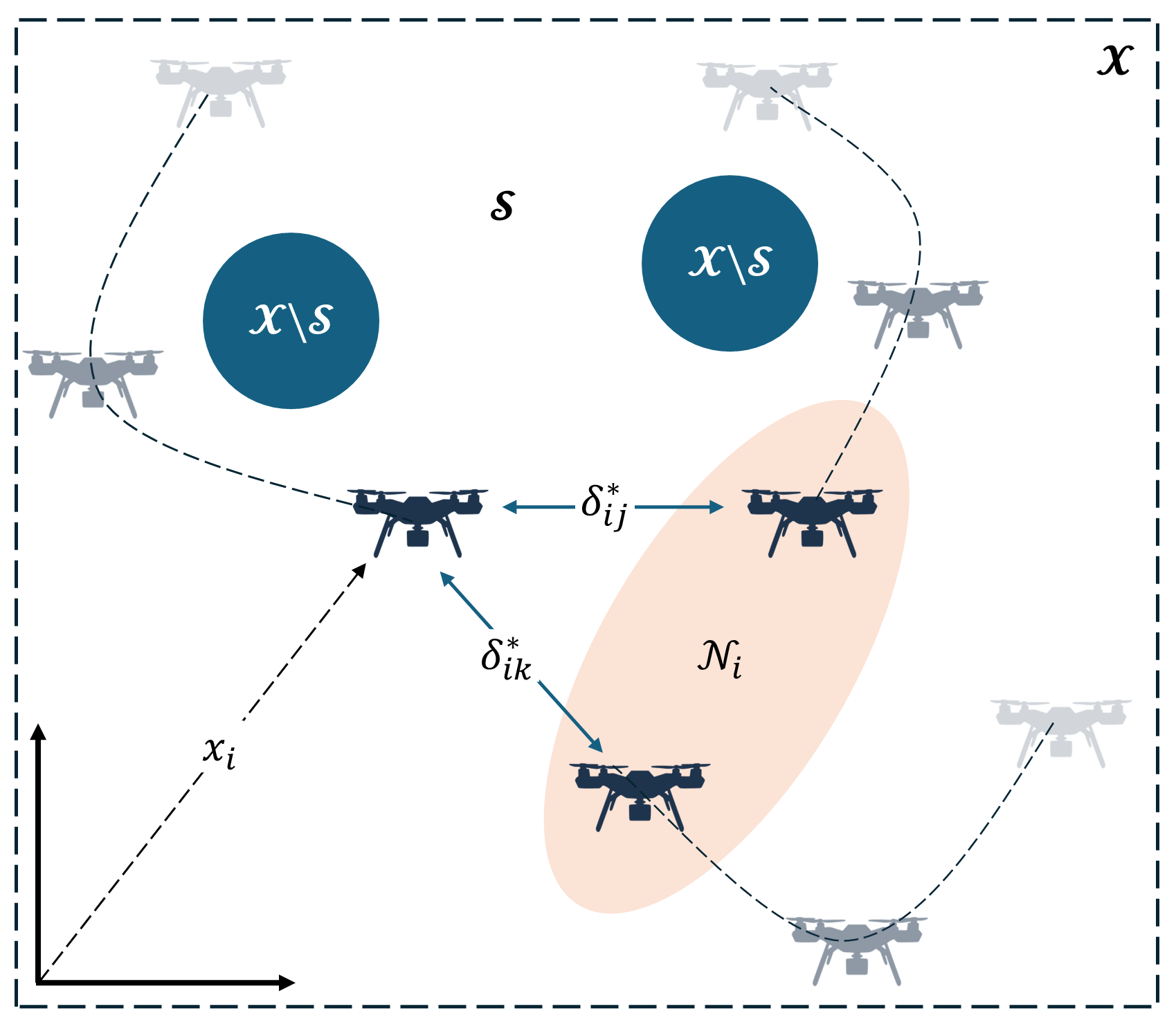
Figure 1: Graphical representation of the proposed method, where a multi-agent system with limited communication needs to converge to a desired formation while avoiding unsafe regions in the presence of parametric uncertainty in the model.

In contrast to the above papers, the authors of [14, 15, 16] have addressed, as in this paper, formation control for distributed MAS amidst obstacles and parametric uncertainties. However the following distinctions can be made: The results in [14] limit the uncertainty to a constant additive disturbance that is unknown. The solutions in [15] and [16] consider general nonlinear dynamics that is unknown, and employ a neural-network based solution. In this paper, we propose an adaptive control solution for static formation control in the presence of parametric uncertainties, obstacles which introduce safety considerations, and limited communication among agents. The unique features of the solution are (i) the use of a Control Barrier Function that shapes the reference input so as to ensure safety, (ii) the use of a reference model that leverages the communication structure, and (iii) an analytically rigorous stability proof that guarantees boundedness of all signals and convergence to the desired formation.

Preliminaries are presented in Section II and the control problem in Section III. The main contribution of this manuscript, the development of an adaptive controller with stability and safety properties, is presented in Section IV. Section V includes numerical simulations.

II Preliminaries

II-A Graph Theory and Multi-Agent Systems Communication

A graph $\mathcal{G}$ is a pair $\{\mathcal{V},\mathcal{E}\}$ where $\mathcal{V}=\{1,\cdots,M\}$ is known as the vertex set which contains the vertices or nodes of the graph (i.e. the agents), and $\mathcal{E}$ is known as the edge set which contains a collection of pairs $(i,j)$ denoting the connectivity or communication between vertices $i$ and $j$ of the vertex set. The set of neighbors of node $i$ is denoted as $\mathcal{N}_{i}\overset{\Delta}{=}\{\ j\ |\ (i.j)\in\mathcal{E}\ \}$.

A graph is called undirected if node $i$ communicates with node $j$ and vice versa, then $(i,j)=(j,i)$. Otherwise, the graph is called directed and node $i$ communicates with node $j$ but node $j$ cannot communicate with node $i$, i.e. $(i,j)\neq(j,i)$. A graph is said to be connected if it has a node to which there exists a (directed) path from every other node. For convenience of the following definitions, throughout this manuscript, only undirected graphs are considered.

Definition 1: The degree matrix $D(\mathcal{G})\in\mathbb{R}^{M\times M}$ of graph $\mathcal{G}$ is a diagonal matrix whose diagonal entries $d_{ii}$ is equal to the number of neighbors of agent $i$, i.e. $|\mathcal{N}_{i}|$.

Definition 2: The adjacency matrix $A(\mathcal{G})\in\mathbb{R}^{M\times M}$ of graph $\mathcal{G}$ is a matrix whose diagonal entries are zero and the off diagonal entries $a_{ij}$ are given by

$$a_{ij}=\begin{cases}-1&\text{if}\ (i,j)\in\mathcal{E}\\ 0&\text{if}\ (i,j)\notin\mathcal{E}\end{cases}$$ (1)

Definition 3: The Laplacian matrix $L(\mathcal{G})\in\mathbb{R}^{M\times M}$ of graph $\mathcal{G}$ is defined as

$$L(\mathcal{G})\overset{\Delta}{=}D(\mathcal{G})-A(\mathcal{G})$$ (2)

Notice that the sum of the rows and columns of the Laplacian matrix add up to zero, therefore $\alpha\mathbf{1}\in\mathbb{R}^{M}$ for all $\alpha\in\mathbb{R}$ lies on the right and left null space of $L$. The Laplacian matrix is a symmetric positive semi-definite matrix. Furthermore, if the graph is connected, the Laplacian has $M-1$ non-zero eigenvalues, i.e. $\lambda_{M}\geq\cdots\geq\lambda_{2}>\lambda_{1}=0$.

II-B The Kronecker Product

The Kronecker Product ($\otimes$) is an operation between two matrices of arbitrary size $A\in\mathbb{R}^{n\times p}$, $B\in\mathbb{R}^{q\times r}$ resulting in a block matrix

$$A\otimes B=\left[\begin{matrix}a_{11}B&\cdots&a_{1p}B\\ \vdots&\ddots&\vdots\\ a_{n1}B&\cdots&a_{np}B\end{matrix}\right]$$ (3)

Relevant properties of the Kronecker product are:

• Mixed-product property: $(A\otimes B)(C\otimes D)=(AC)\otimes(BD)$

• Distributive transpose: $(A\otimes B)^{T}=A^{T}\otimes B^{T}$

• Bilinearity: $A\otimes B+A\otimes C=A\otimes(B+C)$; $B\otimes A+C\otimes A=(B+C)\otimes A$; $(kA)\otimes B=A\otimes(kB)=k(A\otimes B)$

• Definiteness Preservation: Given $A\succeq 0$ and $B\succ 0$, then $(A\otimes B)\succeq 0$ and $(B\otimes A)\succeq 0$. Similarly, given $A\succ 0$ and $B\succ 0$, then $(A\otimes B)\succ 0$ and $(B\otimes A)\succ 0$.

II-C Control Barrier Functions

For the continuous autonomous system

$$\dot{x}(t)=f(x(t))$$ (4)

where $x(t)\in\mathcal{X}\subset\mathbb{R}^{n}$ and $f:\mathcal{X}\rightarrow\mathbb{R}$, safety can be defined in terms of a continuously differentiable function $h:\mathcal{X}\rightarrow\mathbb{R}$ and a set $\mathcal{S}\subset\mathcal{X}$, such that

$$\mathcal{S}\overset{\Delta}{=}\{\ x(t)\in\mathcal{X}\ |\ h(x)\geq 0\ \}$$ (5a)

$$\partial\mathcal{S}\overset{\Delta}{=}\{\ x(t)\in\mathcal{X}\ |\ h(x)=0\ \}$$ (5b)

$$\text{int}(\mathcal{S})\overset{\Delta}{=}\{\ x(t)\in\mathcal{X}\ |\ h(x)>0\ \}$$ (5c)

The following definitions are introduced [17, 18, 19]:

Definition 4: The set $\mathcal{S}$ is positively invariant for the system (4), if for every $x_{0}\in\mathcal{S}$, it follows $x(t)\in\mathcal{S}$ for $x(t_{0})=x_{0}$ and all $t\in\left[t_{0},\infty\right)$.

Definition 5: The set $\mathcal{S}$ is weakly positively invariant for the system (4), if among all the solutions of (4) originating at $x_{0}\in\mathcal{S}$, there exists at least one globally defined solution $x(t)$ which remains inside $\mathcal{S}$ for all $t\in\left[t_{0},\infty\right)$.

Definition 6: Given a set $\mathcal{S}\subset\mathbb{R}^{n}$ and a point $y\in\mathbb{R}^{n}$, the distance from the point to the set is defined as

$$\text{dist}(y,\mathcal{S})=\operatorname*{inf}_{s\in\mathcal{S}}||y-s||$$ (6)

for any relevant norm.

Definition 7: Given a closed set $\mathcal{S}$, the tangent cone to $\mathcal{S}$ at $x$ is defined as

$$T_{\mathcal{S}}=\left\{z:\liminf_{\tau\rightarrow 0}\frac{\text{dist}(x+\tau z,\mathcal{S})}{\tau}=0\right\}$$ (7)

If $\mathcal{S}$ is convex, then $T_{\mathcal{S}}(x)$ is convex and “lim inf” can be replaced by “lim”. Furthermore, if $x\in\text{int}(\mathcal{S})$, then $T_{\mathcal{S}}(x)=\mathbb{R}^{n}$, whereas if $x\notin\mathcal{S}$, then $T_{\mathcal{S}}(x)=\emptyset$, since $\mathcal{S}$ is defined as a closed set. Therefore $T_{\mathcal{S}}(x)$ is only non-trivial on the boundary of $\mathcal{S}$.

Using Definition 7, we state Nagumo’s Invariance Theorem which provides the basis for Control Barrier Functions (CBF).

Theorem 1 [17]: Consider the system defined in (4). Let $\mathcal{S}\subset\mathbb{R}^{n}$ be a closed set. Then, $\mathcal{S}$ is weakly positively invariant for the system if and only if (4) satisfies the following condition:

$$f(x(t))\in T_{\mathcal{S}}(x(t)),\quad\forall x\in\mathcal{S}$$ (8)

The theorem states that if the direction of the dynamics defined in (4) for any $x(t)$ at the boundary of the safe set $\partial\mathcal{S}$ points tangentially or inside to the safe set $\mathcal{S}$, then the trajectory $x(t)$ stays in $\mathcal{S}$.

Definition 8: A continuous function $\alpha:(-b,a)\rightarrow\mathbb{R}$, with $a,b>0$, is an extended class $\mathcal{K}$ function (i.e. $\alpha\in\mathcal{K}$), if $\alpha(0)=0$ and $\alpha$ is strictly monotonically increasing. Furthermore, if $a,b=\infty$, $\lim_{r\to{\infty}}\alpha(r)=\infty,\ \lim_{r\to{-\infty}}\alpha(r)=-\infty$ then $\alpha$ is said to be a class $\mathcal{K}_{\infty}$ function (i.e. $\alpha\in\mathcal{K}_{\infty}$).

Definition 9: For the system considered in (4), a continuously differentiable and convex function $h:\mathcal{X}\rightarrow R$ is a Zeroing Barrier Function (ZBF) for the set $\mathcal{S}$ defined by (5b) and (5c), if there exist $\alpha(h(x(t)))\in\mathcal{K}$ and a set $\mathcal{S}\subset\mathbb{R}^{n}$ such that for all $x\in\mathcal{S}$

$$\dot{h}(x(t))\geq\alpha(h(x(t)))$$ (9)

This requirement over $\mathcal{S}$ is less conservative than the one given on (8).

For a nonlinear control system that is affine in control

$$\dot{x}(t)=f(x(t))+g(x(t))u(t)$$ (10)

where $g(x)$ is Lipschitz and $u(t)\in\mathcal{U}\subseteq\mathbb{R}^{m}$, the notion of CBF [20, 21, 19] can be formulated such that its existence allows the system to be rendered safe with respect to $\mathcal{S}$ in the sense that the set is made weakly positively invariant by some input $u(t)$.

Definition 10: Let $\mathcal{S\subset\mathcal{X}}$ be the zero-superlevel set of $h:\mathcal{X}\rightarrow R$. The function $h$ is a Zeroing Control Barrier Function (ZCBF) for $\mathcal{S}$, if there exists $\alpha(h(x(t)))\in\mathcal{K_{\infty}}$ such that for the system (10) it can be obtained that:

$$\sup_{u\in\mathcal{U}}\left[L_{f}h(x(t))+L_{g}h(x(t))u(t)\right]\geq-\alpha h((x(t)))$$ (11)

for all $x\in\mathcal{S}$, where $L_{\chi}h$ is the Lie derivative of $h$ with respect to $\chi$.

III The Control Problem

In this manuscript we consider static formation control in the presence of obstacle of distributed MAS consisting of $M$ agents indexed by $i\in\mathcal{V}=\{1,\ \cdots,M\}$. The dynamics of agent $i$ are given by

$$\dot{x}_{i}=Ax_{i}+B\left[\Lambda u_{i}+\Xi\omega(x_{i},t)\right]$$ (12)

where $x_{i}\in\mathbb{R}^{n}$ is the state of the agent, $u_{i}\in\mathbb{R}^{m}$ is the control input of the agent. $A\in\mathbb{R}^{n\times n}$ is unknown, $\Lambda\in\mathbb{R}^{m\times m}$ is an unknown diagonal matrix with known sign, and $B\in\mathbb{R}^{n\times m}$ is known and it has full column rank. The term $\Xi\omega(x_{i},t)$ corresponds to nonlinearities present in the system where $\omega(x_{i},t)\in\mathbb{R}^{p}$ is known, but $\Xi\in\mathbb{R}^{n\times p}$ is unknown. For ease of exposition, we assume that $A,\Lambda$ and $\Xi$ are independent of $i$; extensions to the case when they depend on $i$ are straightforward.

Our goal is to determine a safe and stable control solution of the form

$$u_{i}=g(x_{i},x_{j}\ |\ j\in\mathcal{N}_{i})$$ (13)

to enable a MAS to reach a desired formation. Each control policy $g:[\mathbb{R}^{n}]^{|\mathcal{N}_{i}|+1}\rightarrow\mathbb{R}^{m}$ of agent $i$ must depend only on its own state $x_{i}$ and the state of neighboring agents $x_{j}$, $j\in\mathcal{N}_{i}$.

The state constraints for each agent $i$ are captured by the safe set $S_{i}$ for all $i\in\mathcal{V}$ which corresponds to the obstacle-free region of the state space. Associated with this safe set is a ZCBF $h(x_{i})$, which implies the existence of a $u_{i}$ in (12) that guarantees (11). The overall problem statement is therefore the following: given that the initial condition $x_{i}(t_{0})\in\mathcal{S}_{i}$ for all $i\in\mathcal{V}$ and a desired position in the static formation $x_{i}^{\star}\in\mathcal{S}_{i}$ for all $i\in\mathcal{V}$, the problem is to find a control policy (13) that guarantees that $x_{i}(t)\in\mathcal{S}_{i}$ for all $t\geq t_{0}$, and $x_{i}(t)\rightarrow x_{i}^{\star}$.

IV A Safe and Stable Adaptive Controller for Static Formation

The controller that we propose includes an adaptive component and a safety filter. In order to guide the adaptive control design, a reference model is suitably chosen. Each of these components is described below.

IV-A Reference Model

The starting point for the adaptive solution to the MAS formation control is the choice of a reference model which specifies the desired trajectory that the MAS should follow. For this purpose, we propose a reference model dynamics similar to that in [22, 23]:

$$\dot{z}_{i}=A_{m}z_{i}+Bu_{i}$$ (14a)

$$u_{i}=\Theta\left[\sum_{j\in\mathcal{N}_{i}}(z_{j}-z_{i})-\Delta_{i}\right]$$ (14b)

where $A_{m}\in\mathbb{R}^{n\times n}$ is a Hurwitz matrix, $\Delta_{i}(t)\in\mathbb{R}^{n}$ is the reference input vector, and $\Theta$ is a constant control gain. The choice of $\Delta_{i}$ is dictated by the static formation that is of interest. The gain $\Theta$ ensures that the closed-loop reference system remains stable, for a given graph $\mathcal{G}$.

The following theorem clarifies the conditions under which the reference model (14a), (14b) leads to the desired formation [23]. In what follows, $\lambda$ denotes the second smallest eigenvalue of the Laplacian matrix $L(\mathcal{G})$.

Theorem 2: If the graph that captures the communication among agents ($\mathcal{G}$) is connected i.e., $\lambda>0$, then a choice of $\Theta$

$$\Theta=cB^{T}R^{-1}$$ (15)

where

$$A_{m}^{T}R+RA_{m}-2BB^{T}+Q_{0}=0$$ (16a)

$$c\geq 1/\lambda$$ (16b)

for a given $Q_{0}=Q_{0}^{T}\succ 0$ and a choice of the reference input

$$\Delta_{i}(t)=\sum_{j\in\mathcal{N}_{i}}\delta_{ij}^{\star}$$ (17)

for all $t\geq t_{0}$, where $\delta_{ij}^{\star}\overset{\Delta}{=}x_{i}^{\star}-x_{j}^{\star}$, ensures that $z_{i}(t)$ converges to the desired formation $x_{i}^{\star}$, $i\in\mathcal{V}$.

Proof:

We refer the reader to [23]. ∎

IV-B Safety Filter

While Theorem 2 ensures that the reference dynamics in (14a), (14b) achieves a static formation asymptotically, there is no accommodation of the safety requirement that $z_{i}(t)\in S_{i}$ for all $t\geq t_{0}$, and all $i\in\mathcal{V}$. For this purpose, we choose the reference input $\Delta_{i}(t)$ using the QP-ZCBF filter as in [19]:

$$\operatorname*{minimize}_{\Delta_{i}} \quad||\Delta_{i}-\Delta^{\star}_{i}||_{2}^{2}$$ (18)

$$\operatorname*{subject\ to} \quad\frac{\partial h}{\partial z_{i}}^{T}\dot{z}_{i}+\frac{\partial h}{\partial t}\geq-\gamma_{i}h(z_{i})+\upsilon$$

where

$$\Delta_{i}^{\star}\overset{\Delta}{=}\sum_{j\in\mathcal{N}_{i}}\delta_{ij}^{\star}$$ (19)

and we choose the class $\mathcal{K}$ function $\alpha(h(z_{i}(t)))$ as $\gamma_{i}h(z_{i}(t))$ with

$$\gamma_{i}=\gamma_{0}e^{-\beta(h(x_{i}(t))-h(z_{i}(t)))^{2}}$$ (20)

where $\gamma_{0}>0$, $\beta>0$ and $\upsilon\geq 0$ is a safety buffer. (20) is denoted as an Error-Based Relaxation (EBR) [19].

It should be noted that the QP-ZCBF filter in (18)-(20) ensures safety of the reference model, imposing the requirement of forward invariance on $h(z_{i})$ rather than $h(x_{i})$ of the MAS. This helps us with analytical tractability and removes dependence on the unknown parameters.

With the reference model defined in (14), we now introduce the following assumptions and definitions regarding the unknown parameters and nonlinearities in the dynamics:

Assumption 1: The matrix $\text{sign}(\Lambda)\Lambda$ is diagonal and positive definite.

Assumption 2: The nonlinearity $\omega(x_{i},t)$ is a bounded signal for all $t\geq t_{0}$.

Assumption 3: Constant matrix $\theta^{\star}_{1}$ exist such that

$$A+B\Lambda\theta^{\star}_{1}=A_{m}$$ (21)

We also define the following unknown parameters:

$$\theta_{2}^{\star}\overset{\Delta}{=}-\Lambda^{-1}\Theta$$ (22)

$$\theta_{3}^{\star}\overset{\Delta}{=}-\Lambda^{-1}\Xi$$ (23)

IV-C Adaptive Controller

The input $u_{i}$ in (12) is determined using an adaptive control approach:

$$u_{i}=\hat{\theta}^{(i)}_{1}x_{i}+\hat{\theta}^{(i)}_{2}\left[\sum_{j\in\mathcal{N}_{i}}(x_{j}-x_{i})+\Delta_{i}\right]+\hat{\theta}^{(i)}_{3}\omega(x_{i},t)$$ (24)

where $\hat{\theta}^{(i)}_{j}$ for $j=\{1,2,3\}$ are time-varying parameters that are adjusted. We propose the adaptive laws:

$$\dot{\hat{\theta}}^{(i)}_{1}=-\Gamma_{1}\Omega_{i}x_{i}^{T}$$ (25a)

$$\dot{\hat{\theta}}^{(i)}_{2}=-\Gamma_{2}\Omega_{i}\left[\sum_{j\in\mathcal{N}_{i}}\left[(x_{j}-x_{i})-\delta_{ij}^{\star}\right]\right]^{T}$$ (25b)

$$\dot{\hat{\theta}}^{(i)}_{3}=-\Gamma_{3}\Omega_{i}\omega(x_{i},t)^{T}$$ (25c)

where $\Omega_{i}\overset{\Delta}{=}\text{sign}(\Lambda)B^{T}P(x_{i}-z_{i})$, $\Gamma_{j}\in\mathbb{R}^{m\times m}$ are diagonal positive definite gain matrices for all $j=\{1,2,3\}$, and a $Q=Q^{T}\succ 0$ is chosen so that

$$A_{m}^{T}P+PA_{m}+Q=0$$ (26a)

$$R^{-1}BB^{T}P+PBB^{T}R^{-1}\succeq 0$$ (26b)

where $R$ is given by (16a). We make the following important observations about the controller in (24). First, it satisfies the communication constraints in (13). Second, a choice of $\hat{\theta}_{j}^{(i)}=\theta_{j}^{*}$ for all $i=\mathcal{V}$ and $j=\{1,2,3\}$ guarantees that the closed-loop system specified by the plant in (12) and the controller in (24) matches the reference model in (14a)-(14b). The adjustable parameters $\hat{\theta}_{j}^{(i)}$ are introduced for different purposes: $\hat{\theta}^{(i)}_{1}$ is utilized for stabilizing the linear dynamics, $\hat{\theta}^{(i)}_{2}$ is used to enable convergence to the desired formation, while $\hat{\theta}^{(i)}_{3}$ is used to compensate for the nonlinearities.

We now state the first main result of the paper:

Theorem 3: The closed-loop adaptive system defined by the agent dynamics in (12), the control input (24) and the adaptation laws in (25) has globally bounded solutions for any initial conditions $x_{i}(t_{0})$, $\hat{\theta}^{(i)}_{j}(t_{0})$ for all $i\in\mathcal{V}$ and $j=\{1,2,3\}$. Furthermore $x_{i}(t)$ converges to the desired final position $x_{i}^{\star}$ for all $i\in\mathcal{V}$ as $t\rightarrow\infty$.

Proof:

We rewrite the reference model in (14a)-(14b) as

$$\mathbf{\dot{z}}=\left[(I\otimes A_{m})-(L\otimes B\Theta)\right]\mathbf{z}-(I\otimes B\Theta)\Delta$$ (27a)

$$\Delta=\left[\Delta_{1}^{T}\ \cdots\ \Delta_{M}^{T}\right]^{T}$$ (27b)

where $\mathbf{z}\overset{\Delta}{=}[z_{1}^{T},\ \cdots,z_{M}^{T}]^{T}$.

Defining the joint state of the system $\mathbf{x}\overset{\Delta}{=}[x_{1}^{T}\cdots x_{M}^{T}]^{T}$, the error between the true model dynamics and the reference model $\mathbf{e}\overset{\Delta}{=}\mathbf{x}-\mathbf{z}$, and the parameter errors $\tilde{\theta}^{(i)}_{j}\overset{\Delta}{=}\hat{\theta}^{(i)}_{j}-\theta^{\star}_{j}$ for all $i=\mathcal{V}$ and $j=\{1,2,3\}$, the error dynamics can be written as:

$$\mathbf{\dot{e}}=\left[(I\otimes A_{m})-(L\otimes B\Theta)\right]\mathbf{e}+\Psi_{1}\mathbf{x}+\Psi_{2}+\Psi_{3}$$ (28)

where

$$\Psi_{1}=\text{diag}\left(B\Lambda\tilde{\theta}^{(1)}_{1},\cdots,B\Lambda\tilde{\theta}^{(M)}_{1}\right)$$ (29)

$$\Psi_{2}=\left[\begin{matrix}B\Lambda\tilde{\theta}^{(1)}_{2}\sum_{j\in\mathcal{N}_{1}}\left[(x_{j}-x_{1})-\delta_{1j}^{\star}\right]\\ \vdots\\ B\Lambda\tilde{\theta}^{(M)}_{2}\sum_{j\in\mathcal{N}_{M}}\left[(x_{j}-x_{M})-\delta_{Mj}^{\star}\right]\end{matrix}\right]$$ (30)

$$\Psi_{3}=\left[\begin{matrix}B\Lambda\tilde{\theta}^{(1)}_{3}\omega(x_{1},t)\\ \vdots\\ B\Lambda\tilde{\theta}^{(M)}_{3}\omega(x_{M},t)\end{matrix}\right]$$ (31)

We consider the following Lyapunov function candidate:

$$V=\mathbf{e}^{T}\mathbb{P}\mathbf{e}+\sum_{j=1}^{3}\sum_{i=1}^{M}\text{Tr}\left(\tilde{\theta}^{(i)T}_{j}\Gamma_{j}|\Lambda|\tilde{\theta}^{(i)}_{j}\right)$$ (32)

where $\mathbb{P}=I\otimes P\succ 0$ since $P\succ 0$ and is given by (26). This choice for $\mathbb{P}$ is motivated by the fact that it not only needs to guarantee that the system is stable but also needs to ensure that the adaptive laws are only a function of the state of agent $i$ and the state of its neighbors $j\in\mathcal{N}_{i}$.

With this choice of $\mathbb{P}$ and adjusting the control gains as in (25), it can be shown (using the properties of the Kronecker product given in Section II-B and (26b)) that $\dot{V}\leq 0$. Since $V$ is positive definite and radially unbounded and $\dot{V}$ is negative semidefinite, then $\mathbf{e},\ \tilde{\theta}^{(i)}_{j}\in\mathcal{L}_{\infty}$ for all $i=\mathcal{V}$ and $j=\{1,2,3\}$.

Furthermore, because $\dot{V}\leq 0$ we have that $\mathbf{e}\in\mathcal{L}_{2}$, and since $\mathbf{e},\mathbf{\dot{e}}\in\mathcal{L}_{\infty}$, by Barbalat’s Lemma we are able to conclude that $\lim_{t\rightarrow\infty}\mathbf{e}(t)=0$. ∎

We note that the solution for $P$ in (26a)-(26b) can be obtained using LMI approaches, with $Q$ and $Q_{0}$ as decision variables.

IV-D Safe and Stable Formation Control

In the above, we did not address whether or not the overall solution remains safe, that is, all $z_{i}(t)\in\mathcal{S}_{i}$ if $z_{i}(t_{0})\in\mathcal{S}_{i}$. Since the final formation $x_{i}^{\star}\in\mathcal{S}_{i}$, it follows that the adaptive control solution asymptotically reaches the safe set. In order to ensure that the overall solution is always safe, we add the QP-ZCBF filter in the selection of the reference input $\Delta_{i}$. Denoting $\Delta_{i}^{\psi}(t)$ as the solution of (18)-(20), we replace the adaptive control input in (24) by

$$u_{i}=\hat{\theta}^{(i)}_{1}x_{i}+\hat{\theta}^{(i)}_{2}\left[\sum_{j\in\mathcal{N}_{i}}(x_{j}-x_{i})+\Delta_{i}^{\psi}\right]+\hat{\theta}^{(i)}_{3}\omega(x_{i},t)$$ (33)

The overall solution and the second main result of the paper are stated in Theorem 4. As a first step, we discuss the safety of the closed-loop system in comparison of the safety of the reference model.

Since $h$ is a function of only the state of agent $i$ and the parameters of the obstacle, the solutions of the decentralized QP-ZCBF in (18)-(20) is the same as the solution of a centralized QP-ZCBF given by

$$\operatorname*{minimize}_{\Delta} \quad||\Delta-\Delta^{\star}||_{2}^{2}$$ (34)

$$\operatorname*{subject\ to} \quad\frac{\partial\mathbf{h}}{\partial\mathbf{z}}^{T}[\mathbb{A}_{m}\mathbf{z}+\mathbb{B}_{m}\Delta]+\frac{\partial\mathbf{h}}{\partial t}\geq-\gamma\mathbf{h}(\mathbf{z})+\Upsilon$$

where $\mathbb{A}_{m}=(I\otimes A_{m})-(L\otimes B\Theta)$, $\mathbb{B}_{m}=-(I\otimes B\Theta)$, $\Delta^{\star}=\left[\Delta_{1}^{\star T}\ \cdots\ \Delta_{M}^{\star T}\right]^{T}$, $\mathbf{h}=[h(z_{1}),\ \cdots,h(z_{M})]^{T}$ and $\Upsilon=\upsilon\mathbf{1}$. $\mathbf{\gamma}$ is a function of the safety error

$$\mathbf{\gamma}=\text{diag}(\gamma_{0}e^{-\beta(\mathbf{h}(\mathbf{x}(t))-\mathbf{h}(\mathbf{z}(t)))^{2}})$$ (35)

where the exponential function has been overloaded to the vector case. The QP-ZCBF filter ensures that

$$\frac{\partial\mathbf{h}}{\partial\mathbf{z}}^{T}\left[\mathbb{A}_{m}\mathbf{z}+\mathbb{B}_{m}\Delta\right]+\frac{\partial\mathbf{h(\mathbf{z})}}{\partial t}\geq-\gamma\mathbf{h}(\mathbf{z})+\Upsilon$$ (36)

Considering the ZCBF for the joint state

$$\dot{\mathbf{h}}(\mathbf{x}(t))=\frac{\partial\mathbf{h}}{\partial\mathbf{x}}^{T}\left[\mathbb{A}\mathbf{x}+\Phi_{1}\mathbf{x}+\Phi_{2}+\Phi_{3}\right]+\frac{\partial\mathbf{h(\mathbf{x})}}{\partial t}$$ (37)

where $\mathbb{A}=(I\otimes A)$ and

$$\Phi_{1}=\text{diag}\left(B\Lambda\hat{\theta}^{(1)}_{1},\cdots,B\Lambda\hat{\theta}^{(M)}_{1}\right)$$ (38)

$$\Phi_{2}=\left[\begin{matrix}B\Lambda\hat{\theta}^{(1)}_{2}\sum_{j\in\mathcal{N}_{1}}\left[(x_{j}-x_{1})-\delta_{1j}^{\star}\right]\\ \vdots\\ B\Lambda\hat{\theta}^{(M)}_{2}\sum_{j\in\mathcal{N}_{M}}\left[(x_{j}-x_{M})-\delta_{Mj}^{\star}\right]\end{matrix}\right]$$ (39)

$$\Phi_{3}=\left[\begin{matrix}B\Lambda\hat{\theta}^{(1)}_{3}\omega(x_{1},t)\\ \vdots\\ B\Lambda\hat{\theta}^{(M)}_{3}\omega(x_{M},t)\end{matrix}\right]$$ (40)

Following a similar approach as in [19], using the relations (36) and (37), it can be shown that

$$\dot{\mathbf{h}}(\mathbf{x}(t))\geq-\gamma\mathbf{h}(\mathbf{x})+\Upsilon+\underbrace{\left[\frac{\partial\mathbf{h(\mathbf{x})}}{\partial t}-\frac{\partial\mathbf{h(\mathbf{z})}}{\partial t}\right]}_{\Delta_{\partial t}}+\mathbf{F}(|\mathbf{e}|,|\tilde{\mathbf{u}}|)$$ (41)

where $\mathbf{F}$ is a function of the magnitude of the error $\mathbf{e}$ and the output error $\tilde{\mathbf{u}}\overset{\Delta}{=}[\tilde{u}_{1}^{T}\cdots\tilde{u}_{M}^{T}]^{T}$, where $\tilde{u}_{i}\overset{\Delta}{=}u_{i}(t)-u_{i}^{\star}$, for all $i=\mathcal{V}$ and

$$u_{i}^{\star}\overset{\Delta}{=}\hat{\theta}^{\star}_{1}x_{i}+\hat{\theta}^{\star}_{2}\left[\sum_{j\in\mathcal{N}_{i}}(x_{j}-x_{i})+\Delta_{i}^{\psi}\right]+\hat{\theta}^{\star}_{3}\omega(x_{i},t)$$ (42)

Since $\tilde{\theta}^{(i)}_{j}\in\mathcal{L}_{\infty}$ for all $i=\mathcal{V}$ and $j=\{1,2,3\}$, and the signals $\omega(x_{i},t)$ and $\Delta_{i}^{\psi}(t)$ are bounded, then $\tilde{u}_{i}\in\mathcal{L}_{\infty}$ for all $i=\mathcal{V}$. From (28) and the definition of $\tilde{\mathbf{u}}$, it can be shown that $\tilde{\mathbf{u}}$ is the input into an LTI system, whose state is $\mathbf{e}$ and has bounded derivative, $\dot{\mathbf{e}}$. It follows that that $\lim_{t\rightarrow\infty}\tilde{\mathbf{u}}(t)=0$ [24].

The inequality in (41) suggests that the safety of the closed-loop adaptive system will be ensured for $t\geq t_{0}+T$, where $T$ is a finite interval, as $\mathbf{F}(t)\rightarrow 0$ and $\Delta_{\partial t}(t)\rightarrow 0$ as $t\rightarrow\infty$. Hence, $\Upsilon\geq\mathbf{F}(t)+\Delta_{\partial t}$ holds for all $t\geq t_{0}+T$. Consequently, the closed-loop adaptive system will remain safe for all $t\geq t_{0}$ if

$$\mathbf{h}(\mathbf{x}(t))\geq\mathbf{h}_{0},\quad\forall t\geq[t_{0},t_{0}+T]$$ (43)

where

$$\mathbf{h}_{0}\overset{\Delta}{=}\gamma^{-1}(\mathbf{F}_{max}+\Delta_{\partial t,max})$$ (44)

and

$$\mathbf{F}_{max}=\max_{t\in\left[t_{0},t_{0}+T\right]}\mathbf{F}(t)$$ (45)

$$\Delta_{\partial t,max}=\max_{t\in\left[t_{0},t_{0}+T\right]}\Delta_{\partial t}(t)$$ (46)

As $\mathbf{F}(t)$ is bounded since $\mathbf{e}$ and $\tilde{\mathbf{u}}$ are bounded as shown in the proof of Theorem 3, then $\mathbf{F}_{max}$ exists. Since $\frac{\partial\mathbf{h}}{\partial t}$ is bounded, then $\Delta_{\partial t,max}$ also exists. Condition (43) essentially implies that there is a separation between the period of adaptation and the time at which the system approaches its limit of safety. The choice of $\gamma$ tightens the safety constraints when $\mathbf{e}$ is large, and relaxes as $\mathbf{e}\rightarrow 0$.

Theorem 4: The closed-loop adaptive system defined by (33),(24),(25), and the safety filter (18)-(20) guarantees that $x_{i}(t)\in\mathcal{S}_{i}$ for all $t\geq t_{0}$, if $x_{i}(t_{0})\in\mathcal{S}_{i}$ and (43) is satisfied. Further, $x_{i}(t)\rightarrow x_{i}^{\star}$ as $t\rightarrow\infty$ if $x_{i}^{\star}\in\mathcal{S}_{i}$ for all $i\in\mathcal{V}$.

Proof:

By the result shown in [19], since the reference model $\mathbf{z}(t)$ is rendered safe as ensured by the centralized QP-ZCBF (34), and condition (43) is satisfied, where $\mathbf{F}_{max}$ and $\Delta_{\partial t,max}$ are defined by (45) and (46), respectively, then the closed-loop system $\mathbf{x}(t)$ is also guaranteed to be safe.

Since the formation is safe, by the result of Theorem 3 $z_{i}(t)\rightarrow x_{i}^{\star}$ and therefore $x_{i}(t)\rightarrow x_{i}^{\star}$ as $t\rightarrow\infty$. ∎

V Simulation

The proposed controller is applied to a two-dimensional obstacle avoidance problem. The dynamics of each agent are given by

$$\left[\begin{matrix}\dot{x}_{i}\\ \dot{y}_{i}\end{matrix}\right]=\left[\begin{matrix}0.25&0\\ 0&0.25\end{matrix}\right]\left[\begin{matrix}x_{i}\\ y_{i}\end{matrix}\right]+\left[\begin{matrix}1.5&0\\ 0&1.5\end{matrix}\right]\left[\Lambda u_{i}+\Xi\omega\right]$$ (47)

where actuation has been compromised ($\Lambda=0.9I$) and the nonlinearities are characterized by

$$\Xi=\left[\begin{matrix}0.25&-0.1\\ -0.1&0.25\end{matrix}\right]$$ (48)

$$\omega(x_{i},y_{i},t)=\left[\omega_{1}(x_{i},t)\ \omega_{2}(y_{i},t)\right]^{T}$$ (49a)

$$\omega_{1}(x_{i},t)=\begin{cases}\cos(5t)&x_{i}\geq 0.75\\ -\cos(5t)&x_{i}\leq-0.75\\ 0&\text{otherwise}\end{cases}$$ (49b)

$$\omega_{2}(y_{i},t)=\begin{cases}\sin(5t)&y_{i}\geq 0.75\\ -\sin(5t)&y_{i}\leq-0.75\\ 0&\text{otherwise}\end{cases}$$ (49c)

such that $x_{i}$ and $y_{i}$ are the horizontal and vertical positions of the agents, respectively. The reference model is defined by

$$A_{m}=\left[\begin{matrix}-2&0\\ 0&-2\end{matrix}\right]$$ (50)

and the communication graph shown in Fig. 2. To guarantee the safety of each agent, the following CBF constraint is chosen for each obstacle

$$h_{k}(x_{i},y_{i})=(x_{i}-\bar{x}_{k})^{2}+(y_{i}-\bar{y}_{k})^{2}-r_{k}^{2}\geq 0$$ (51)

where $(\bar{x}_{k},\bar{y}_{k})$ and $r_{k}$ are the position and radius of the k-th circular obstacle.

Fig. 3 shows the trajectories of the reference model as described in (27) with the above-mentioned parameters; Fig. 4 shows the trajectories of the agents only using the adaptation controller as described in Section IV-C; and Fig. 5 shows our porposed adaptive controller with control barrier functions. Notice that only using the adaptive controller, agents 1, 3 and 4 collide with the obstacles along the trajectory (Fig. 4). When using the proposed approach, the agents reach the desired formation without collision (Fig. 5). We refer the reader to aaclab.mit.edu for animations of the results in Fig. 4 and Fig. 5. It’s crucial to emphasize that the system successfully accomplishes the task without collisions, despite operating under unstable dynamics and partially known nonlinearities. Furthermore, it manages to do so even when the actuation is compromised in an unknown manner.

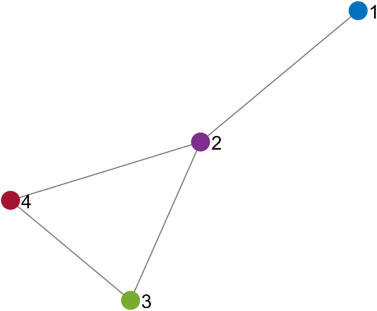
Figure 2: Multi-agent system communication graph for the obstacle avoidance example.

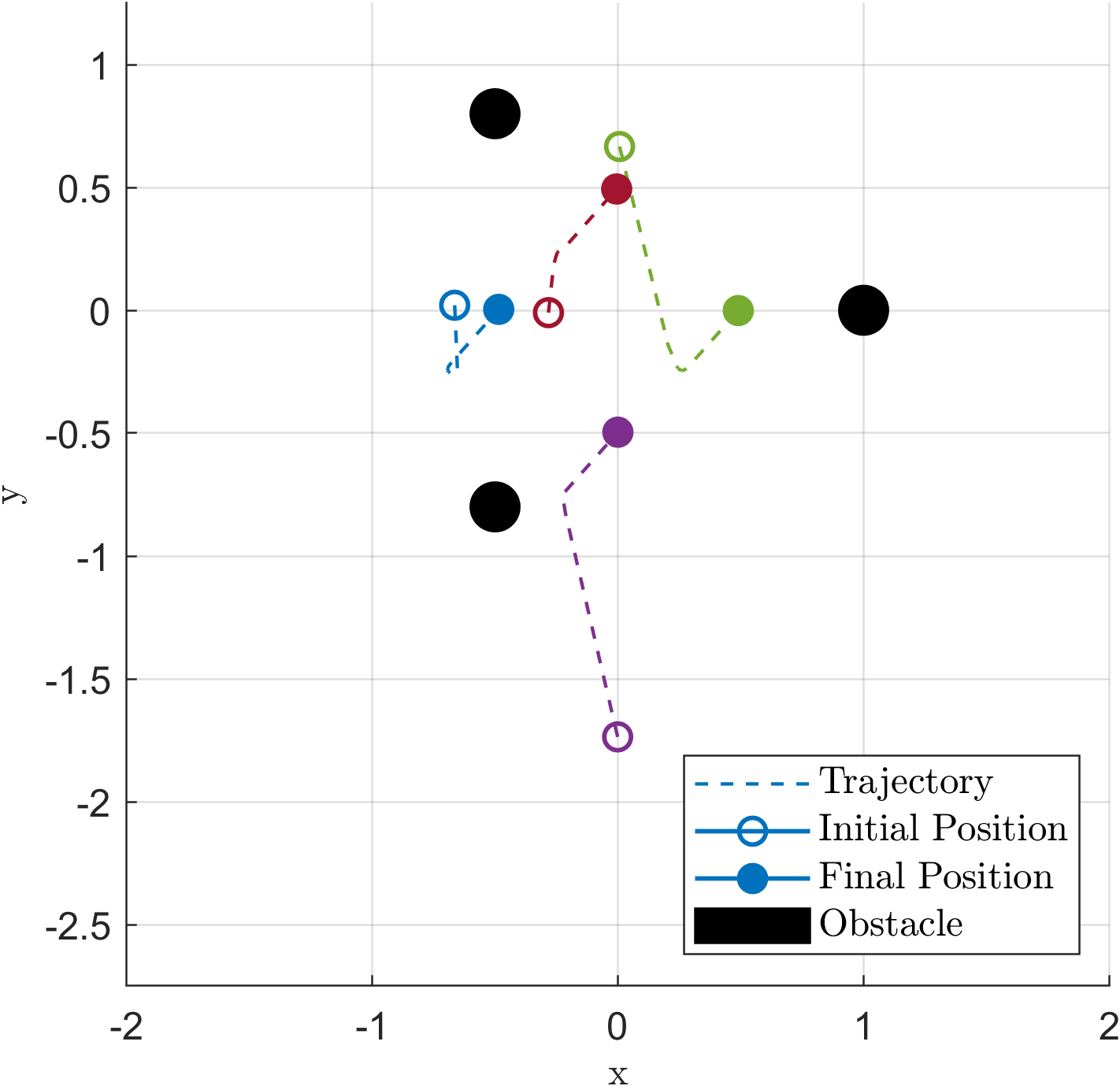
Figure 3: Trajectory of the reference model for the multi-agent system in the presence of obstacles.

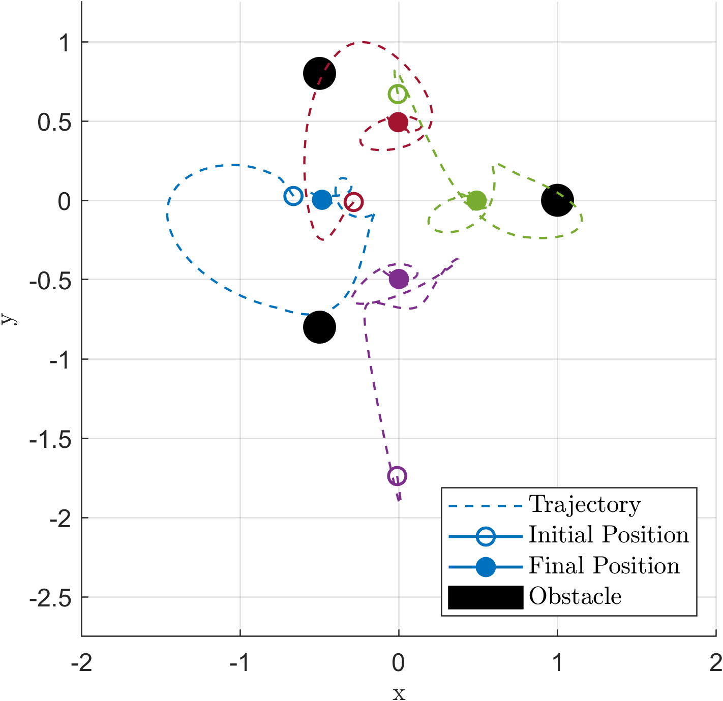
Figure 4: Trajectory of the multi-agent system in the presence of obstacles and only using the adaptive controller.

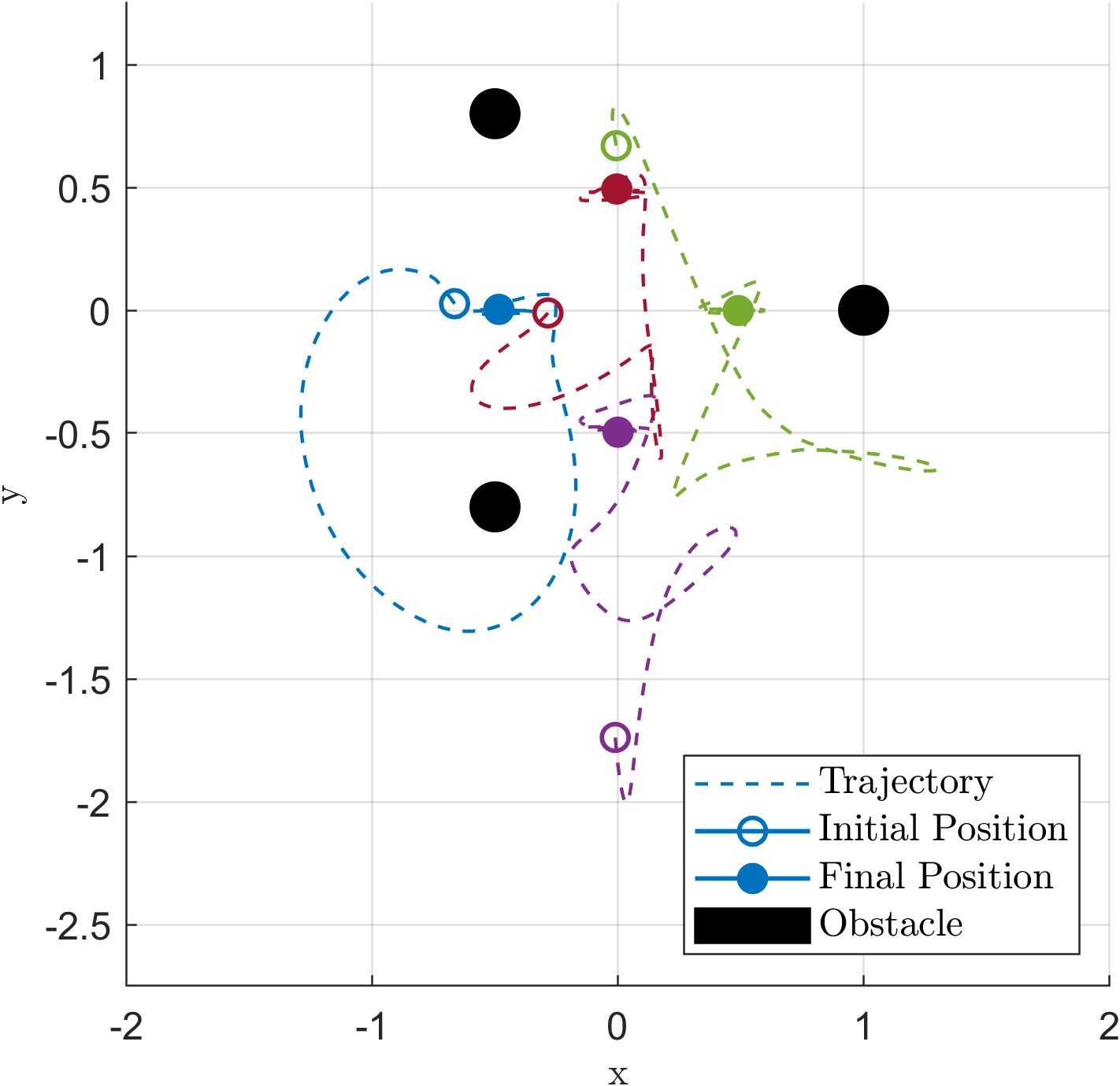
Figure 5: Trajectory of the multi-agent system in the presence of obstacles and using the proposed adaptive controller with control barrier functions.

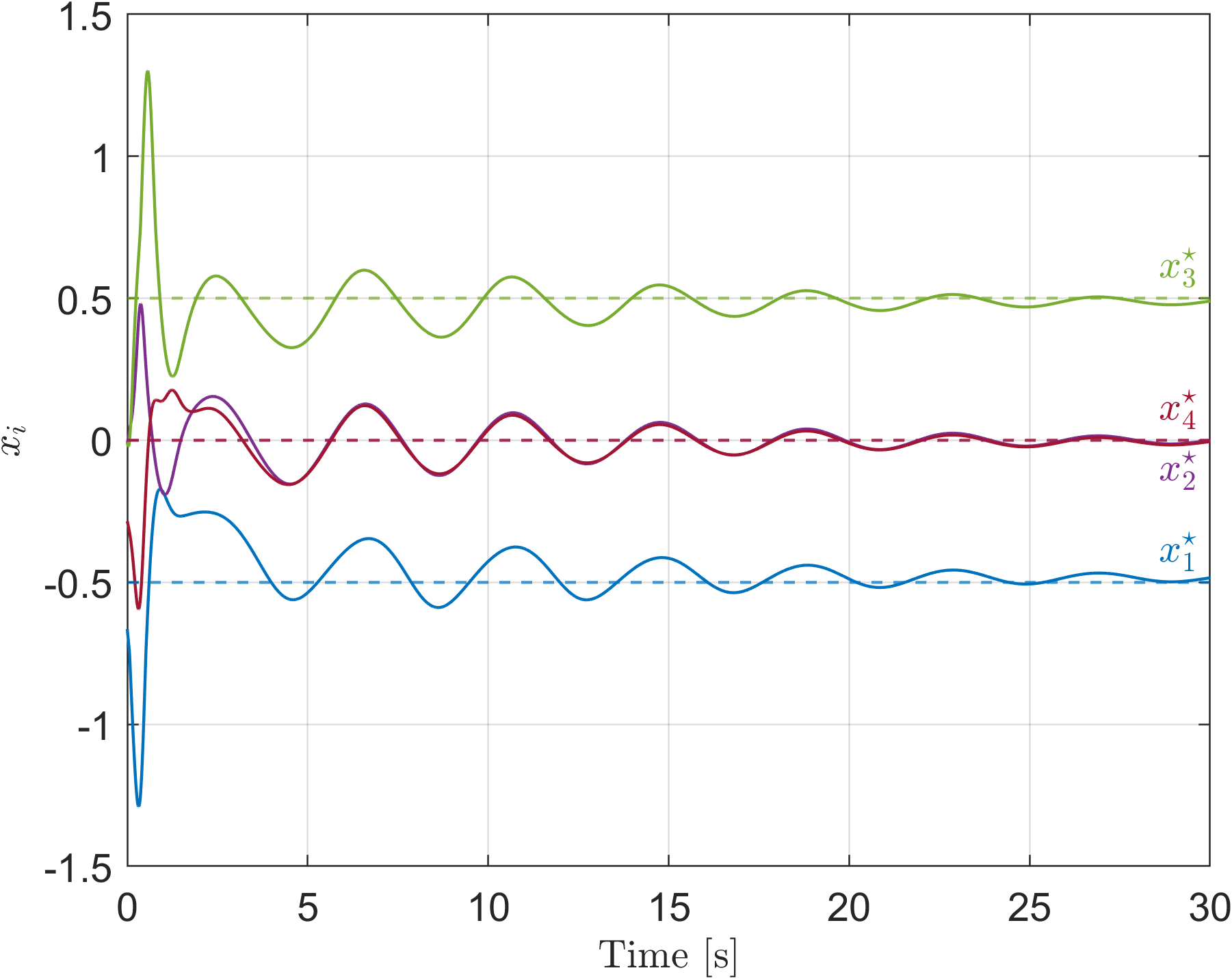
Figure 6: Trajectories of the horizontal position of all agents as a function of time with the proposed adaptive controller and control barrier functions.

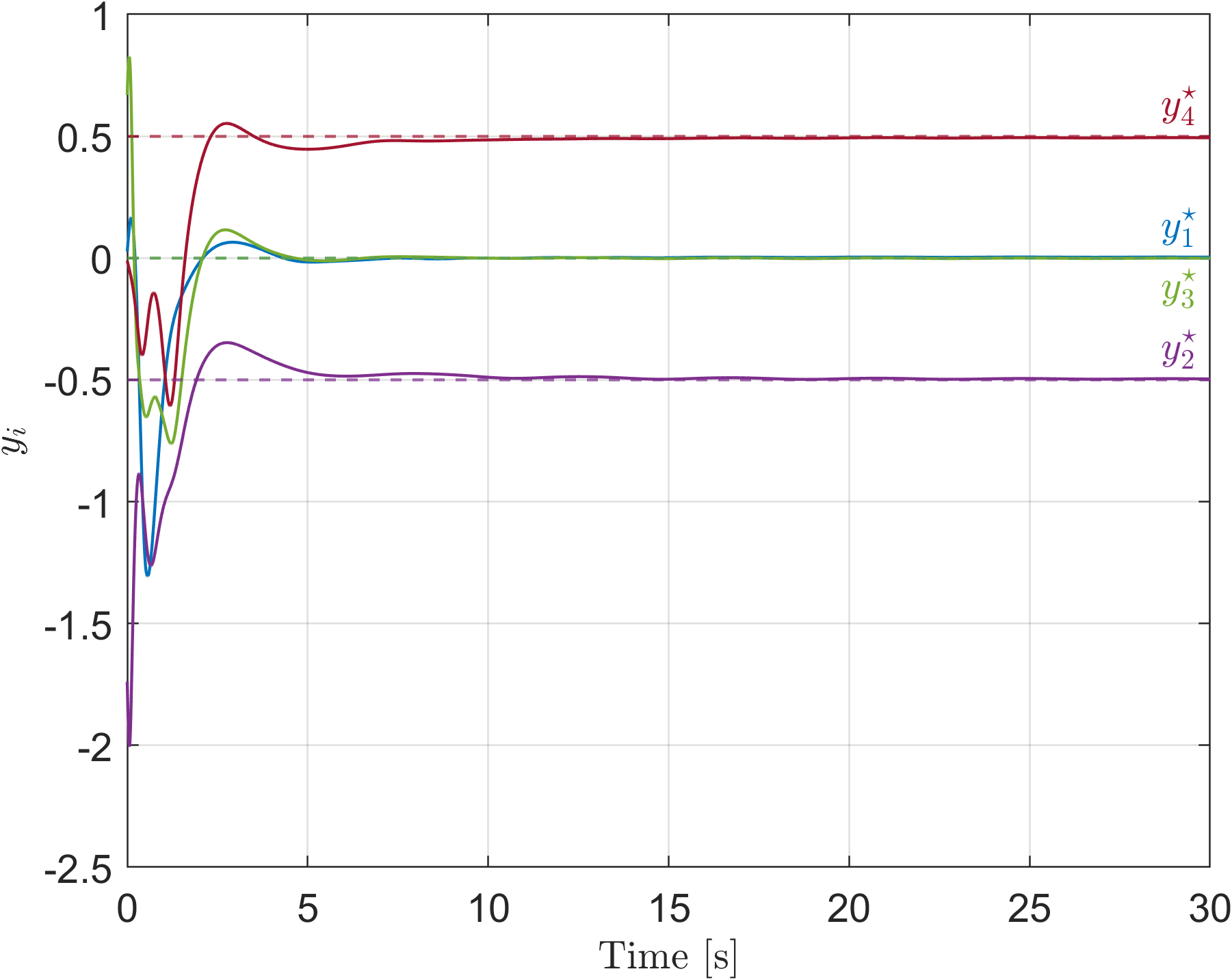
Figure 7: Trajectories of the vertical position of all agents as a function of time with the proposed adaptive controller and control barrier functions.

VI Conclusions

In this paper, we consider the problem of static formation control with distributed MAS in the presence of parametric uncertainties and limited communication. The class of problems considered is nonlinear systems that are feedback linearizable, with states accessible for measurement. The goal is to ensure that the MAS stay inside a safe set with the overall closed-loop system remaining stable while meeting the formation goals. Our approach is a combination of adaptive control and control barrier functions, with the former providing a means for accommodating to parametric uncertainties and the latter providing a safety filter that ensures that the states stay within a safe region and remain forward-invariant. The innovations are the design of a calibrated control barrier function designed using an underlying reference model which serves as a desired dynamics that ensures a safe formation. Theoretical results are provided that guarantee global boundedness and safety against obstacles in the overall state space, and convergence to the desired formation. Numerical results show the effectiveness of the proposed method.

References

• [1] E. Lavretsky, N. Hovakimyan, A. Calise, and V. Stepanyan, “Adaptive Vortex Seeking Formation Flight Neurocontrol,” in AIAA Guidance, Navigation, and Control Conference and Exhibit, (Reston, Virigina), American Institute of Aeronautics and Astronautics, 8 2003.
• [2] Z. T. Dydek, A. M. Annaswamy, and E. Lavretsky, “Adaptive configuration control of multiple UAVs,” Control Engineering Practice, vol. 21, no. 8, pp. 1043–1052, 2013.
• [3] R. Li, L. Zhang, L. Han, and J. Wang, “Multiple Vehicle Formation Control Based on Robust Adaptive Control Algorithm,” IEEE Intelligent Transportation Systems Magazine, vol. 9, no. 2, pp. 41–51, 2017.
• [4] X. Cai and M. d. Queiroz, “Adaptive Rigidity-Based Formation Control for Multirobotic Vehicles With Dynamics,” IEEE Transactions on Control Systems Technology, vol. 23, no. 1, pp. 389–396, 2015.
• [5] N. Xuan-Mung and S. K. Hong, “Robust adaptive formation control of quadcopters based on a leader–follower approach,” International Journal of Advanced Robotic Systems, vol. 16, p. 1729881419862733, 7 2019.
• [6] W. Wang, J. Huang, C. Wen, and H. Fan, “Distributed adaptive control for consensus tracking with application to formation control of nonholonomic mobile robots,” Automatica, vol. 50, no. 4, pp. 1254–1263, 2014.
• [7] L. Dai, Q. Cao, Y. Xia, and Y. Gao, “Distributed MPC for formation of multi-agent systems with collision avoidance and obstacle avoidance,” Journal of the Franklin Institute, vol. 354, no. 4, pp. 2068–2085, 2017.
• [8] A. Wasik, J. N. Pereira, R. Ventura, P. U. Lima, and A. Martinoli, “Graph-based distributed control for adaptive multi-robot patrolling through local formation transformation,” in 2016 IEEE/RSJ International Conference on Intelligent Robots and Systems (IROS), pp. 1721–1728, 2016.
• [9] J. F. Flores-Resendiz, D. Avilés, and E. Aranda-Bricaire, “Formation Control for Second-Order Multi-Agent Systems with Collision Avoidance,” Machines, vol. 11, no. 2, 2023.
• [10] J. Fu, G. Wen, X. Yu, and Z. G. Wu, “Distributed Formation Navigation of Constrained Second-Order Multiagent Systems With Collision Avoidance and Connectivity Maintenance,” IEEE Transactions on Cybernetics, vol. 52, no. 4, pp. 2149–2162, 2022.
• [11] L. Wang, A. D. Ames, and M. Egerstedt, “Safety Barrier Certificates for Collisions-Free Multirobot Systems,” IEEE Transactions on Robotics, vol. 33, no. 3, pp. 661–674, 2017.
• [12] Y. Zhou, F. Lu, G. Pu, X. Ma, R. Sun, H. Y. Chen, and X. Li, “Adaptive Leader-Follower Formation Control and Obstacle Avoidance via Deep Reinforcement Learning,” in 2019 IEEE/RSJ International Conference on Intelligent Robots and Systems (IROS), pp. 4273–4280, 2019.
• [13] A. Parvareh, M. Naderi Soorki, and A. Azizi, “The Robust Adaptive Control of Leader–Follower Formation in Mobile Robots with Dynamic Obstacle Avoidance,” Mathematics, vol. 11, no. 20, 2023.
• [14] X. Yang and X. Fan, “A Distributed Formation Control Scheme with Obstacle Avoidance for Multiagent Systems,” Mathematical Problems in Engineering, vol. 2019, p. 3252303, 2019.
• [15] X. Ge, Q. L. Han, J. Wang, and X. M. Zhang, “A Scalable Adaptive Approach to Multi-Vehicle Formation Control with Obstacle Avoidance,” IEEE/CAA Journal of Automatica Sinica, vol. 9, no. 6, pp. 990–1004, 2022.
• [16] Q. Shi, T. Li, J. Li, C. L. P. Chen, Y. Xiao, and Q. Shan, “Adaptive leader-following formation control with collision avoidance for a class of second-order nonlinear multi-agent systems,” Neurocomputing, vol. 350, pp. 282–290, 2019.
• [17] M. NAGUMO, “Ueber die Lage der Integralkurven gewoehlicher Differentialgleichungen,” Proceedings of the Physico-Mathematical Society of Japan. 3rd Series, vol. 24, pp. 551–559, 1942.
• [18] F. Blanchini, “Set invariance in control,” Automatica, vol. 35, no. 11, pp. 1747–1767, 1999.
• [19] J. Autenrieb and A. Annaswamy, “Safe and Stable Adaptive Control for a Class of Dynamic Systems,” in 2023 62nd IEEE Conference on Decision and Control (CDC), pp. 5059–5066, 2023.
• [20] S. Prajna and A. Jadbabaie, “Safety Verification of Hybrid Systems Using Barrier Certificates,” in Hybrid Systems: Computation and Control (R. Alur and G. J. Pappas, eds.), (Berlin, Heidelberg), pp. 477–492, Springer Berlin Heidelberg, 2004.
• [21] A. D. Ames, J. W. Grizzle, and P. Tabuada, “Control barrier function based quadratic programs with application to adaptive cruise control,” in 53rd IEEE Conference on Decision and Control, pp. 6271–6278, 2014.
• [22] R. Olfati-Saber and R. M. Murray, “Consensus problems in networks of agents with switching topology and time-delays,” IEEE Transactions on Automatic Control, vol. 49, no. 9, pp. 1520–1533, 2004.
• [23] Z. Li, Z. Duan, G. Chen, and L. Huang, “Consensus of Multiagent Systems and Synchronization of Complex Networks: A Unified Viewpoint,” IEEE Transactions on Circuits and Systems I: Regular Papers, vol. 57, no. 1, pp. 213–224, 2010.
• [24] A. M. Annaswamy, A. Guha, Y. Cui, S. Tang, P. A. Fisher, and J. E. Gaudio, “Online Algorithms and Policies Using Adaptive and Machine Learning Approaches,” 5 2021.