Constraint Preconditioning and Parameter Selection for a First-Order Primal-Dual Method applied to Model Predictive Control

Abstract

Many techniques for real-time trajectory optimization and control require the solution of optimization problems at high frequencies. However, ill-conditioning in the optimization problem can significantly reduce the speed of first-order primal-dual optimization algorithms. We introduce a preconditioning technique and step-size heuristic for Proportional-Integral Projected Gradient (PIPG), a first-order primal-dual algorithm. The preconditioning technique, based on the QR factorization, aims to reduce the condition number of the KKT matrix associated with the optimization problem. Our step-size selection heuristic chooses step-sizes to minimize the upper bound on the convergence of the primal-dual gap for the optimization problem. These algorithms are tested on two model predictive control problem examples and show a solve-time reduction of at least 3.6x.

I INTRODUCTION

Solving optimal control problems in real-time is at the heart of model predictive control (MPC). This control scheme is optimization-based, where we solve a fixed time horizon optimal control problem recursively to generate state and control trajectories which satisfy relevant system constraints while minimizing a predefined cost function.

In this paper, we consider optimal control problems in the form

$$\underset{z}{\mathrm{minimize}}\quad \frac{1}{2}z^{\top}Pz+q^{\top}z$$ (1a)

$$\mathrm{subject\;to}\quad Hz-g=0$$ (1b)

$$z\in\mathbb{D}$$ (1c)

where $H\in\mathbb{R}^{m\times n}$, $m\leq n$, and $P\succ 0$. Constraint 1b contains the linear dynamics and set $\mathbb{D}$ contains state and control constraints. We assume that set $\mathbb{D}$ is the Cartesian product of sets that have closed-form projections, such as balls, boxes, second-order cones, half-spaces, and the intersection of a ball and second-order cone [1, 2]. This assumption applies to many typical state and control constraints in MPC [3].

First-order optimization algorithms are popular for solving MPC problems due to their ability to warm-start from any prescribed solution (e.g., one that can be obtained from the previous solution in a recursive MPC scheme), which greatly reduces solve-times and per-iteration computational cost. Unlike second-order methods, first-order methods do not require expensive matrix factorizations, making them attractive for resource constrained embedded systems [4].

However, ill-conditioned optimization problems degrade the performance of methods in this class. Consequently, first-order optimization algorithms use preconditioning and parameter selection to improve their convergence behavior. Preconditioning transforms the given optimization problem into an equivalent problem which is able to be solved in fewer iterations. This is achieved by performing a change of variables or transforming the constraints of the problem to reduce the condition number of a matrix related to the optimization problem, such as the KKT matrix. Whereas preconditioning modifies the given optimization problem, parameter selection modifies the optimization algorithm itself. Parameter selection involves choosing parameters of an optimization algorithm such as step-size or relaxation parameters for fastest convergence [5].

Modified Ruiz equilibriation [6] and the hypersphere preconditioner [7] are two existing preconditioning techniques for first-order primal-dual algorithms. These preconditioners aim to reduce the condition number of the KKT matrix. Both perform a change of variables and additionally, modified Ruiz equilibriation scales the constraints with a diagonal matrix. These two preconditioner transform set $\mathbb{D}$ in Problem 1 since they both employ a change of variables. This requires special structure in the matrices defining the change of variables in order to preserve closed-form projections onto $\mathbb{D}$, which is needed to solve Problem 1 by using Proportional-Integral Projected Gradient (pipg), a first-order primal-dual optimization algorithm [8, 9, 10].

Our first contribution is the development of the QR preconditioner. This proposed preconditioner does not perform a change of variables, meaning set $\mathbb{D}$ is not transformed and consequently closed-form projections are preserved. Instead, the QR preconditioner transforms the equality constraints by scaling them with a triangular matrix to minimize the condition number of the KKT matrix. Since a triangular matrix is used for transforming the constraints as opposed to a diagonal matrix, the QR preconditioner has more degrees of freedom to transform the constraints than modified Ruiz equilibriation. The QR preconditioner requires a matrix factorization to perform this constraint transformation, unlike the aforementioned preconditioners, making it more computationally expensive. However, in our numerical examples the factorization time was a small percentage of the overall solve-time. Additionally, in settings requiring the solution of multiple optimization problems with identical equality constraints, such as quasi-convex optimization and MPC, performing the preconditioning offline and solving the preconditioned problem online will result in improved real-time performance.

Our second contribution is a step-size selection heuristic for pipg. For fastest convergence, pipg requires carefully selecting step sizes, a process that is currently manually tuned. We eliminate manual tuning of step-sizes by introducing a step-size selection heuristic based on choosing step-sizes to minimize the upper bound on the primal-dual gap.

I-A Related work

In this section we will discuss two existing preconditioning methods.

The hypersphere preconditioner [7] performs a change of variables to make the Hessian of the objective function some positive multiple of the identity matrix, making the objective function perfectly conditioned. This preconditioner avoids transforming the constraints. It is applicable to pipg when the Hessian of the objective function is diagonal or has an easy to compute Cholesky factorization, and the change of variables induced by the preconditioner preserves the ability to project onto set $\mathbb{D}$ in closed-form.

Modified Ruiz equilibration [6] preconditions the objective function and transforms the constraints by performing a linear change of variables with a diagonal matrix and scaling the constraints with a diagonal matrix to make the preconditioned KKT matrix have equal row and column norms, a heuristic for good conditioning. Similar to the hypersphere preconditioner, to be applicable to pipg the change of variables induced must preserve the ability to project onto set $\mathbb{D}$ in closed-form.

I-B Notation

We denote the $n\times 1$ vector of zeros as $0_{n}$, the $m\times n$ matrix of zeros as $0_{m\times n}$, the $n\times n$ identity matrix as $I_{n}$, the Euclidean projection of point $z$ onto the convex set $\mathbb{D}$ as $\Pi_{\mathbb{D}}[z]$, the concatenation of vectors $u$ and $v$ as $(u,v)$, the vector formed from the $i^{th}$ through the $j^{th}$ component of $z$ as $z^{i:j}$, and the Euclidean norm of a vector $z$ as $\|z\|:=\sqrt{z^{\top}z}$.

II Proportional-Integral Projected Gradient

Proportional-Integral Projected Gradient (pipg), shown in Algorithm 1, is a first-order primal-dual conic optimization algorithm capable of infeasibility detection. This algorithm is specialized to handle common constraints sets which arise in optimal control problems, such as boxes, balls, and second-order cones, via closed-form projections [8, 9, 10]. PIPG has been demonstrated to be faster than many state-of-the art optimization solvers such as ecos, mosek, gurobi, and osqp [10]. pipg has been applied extensively to trajectory optimization problems including three-degree-of-freedom (DoF) powered-descent guidance and has been used as a subproblem solver within sequential convex programming for multi-phase powered-descent guidance, 6-DoF powered-descent-guidance, and spacecraft rendezvous problems [7, 11, 12, 13, 14].

Algorithm 1 PIPG

$k_{\max},\alpha,\beta,z^{1}\in\mathbb{D},v^{1}$. $z^{k}$. $k=1,2,\ldots,k_{\max}-1$

1:$w^{k+1}=v^{k}+\beta(Hz^{k}-g)$

2:$z^{k+1}=\Pi_{\mathbb{D}}[z^{k}-\alpha(Pz^{k}+q+H^{\top}w^{k+1})]$

3:$v^{k+1}=w^{k+1}+\beta H(z^{k+1}-z^{k})$

In Algorithm 1, $z^{k}$ and $w^{k}$ are the iterates of the primal and dual variables respectively. Thus, we refer to $\alpha$ and $\beta$ as the primal and dual step-sizes. For the convergence results to hold for pipg, the primal and dual step-sizes must satisfy the algebraic relationship

$$\alpha(\lambda_{\mathrm{max}}+\sigma\beta)<1.$$

We parameterize this family of step-sizes with $\gamma>0$ as

$$\alpha<\frac{1}{\lambda_{\mathrm{max}}+\gamma},\quad\beta=\frac{\gamma}{\sigma}$$ (2)

where $\lambda_{\mathrm{max}}$ is the maximum eigenvalue of $P$ and $\sigma$ is the maximum eigenvalue of $H^{\top}H$. In practice we choose $\alpha$ to be equal to the upper bound and do not observe convergence issues. We will discuss how to choose $\gamma$ in Section IV.

III QR PRECONDITIONER

In this section, we derive and provide a geometric interpretation for the QR preconditioner.

III-A Derivation

First, we derive a preconditioner that only modifies Constraint 1b of Problem 1 and minimizes the condition number of the KKT matrix. First, we need the following assumptions on the constraint matrix $H$ and the Hessian of the objective function $P$.

Assumption 1

$H\in\mathbb{R}^{m\times n}$ has full row rank.

Assumption 2

$P$ is positive definite and has maximum and minimum eigenvalues $\lambda_{\mathrm{max}}$ and $\lambda_{\mathrm{min}}$ respectively.

The KKT conditions of Problem 1 are as follows

$$\underbrace{\begin{bmatrix}P&H^{\top}\\ H&0_{m\times m}\end{bmatrix}}_{\mathcal{K}}\begin{bmatrix}x^{\star}\\ w^{\star}\end{bmatrix}+\begin{bmatrix}q\\ -g\end{bmatrix}\in\begin{bmatrix}-\mathbb{N}_{\mathbb{D}}(z^{\star})\\ \{0_{m}\}\end{bmatrix}$$ (3)

where $z^{\star}$ and $w^{\star}$ are the optimal primal and dual solutions respectively and $\mathbb{N}_{\mathbb{D}}(z^{\star})$ is the normal cone of set $\mathbb{D}$ at $z^{\star}$. We denote the KKT matrix as $\mathcal{K}$.

If Assumptions 1 and 2 hold and $\sigma_{\mathrm{max}}$ and $\sigma_{\mathrm{min}}$ are the maximum and minimum singular values of $H$, the eigenvalues of $\mathcal{K}$ lie in the following set [15]

$$\lambda(\mathcal{K})\subset\mathcal{I}^{-}\cup\mathcal{I}^{+}\\$$

where

$$\begin{split}\mathcal{I}^{-}=\left[\frac{1}{2}\left(\lambda_{\mathrm{min}}-\sqrt{\lambda_{\mathrm{min}}^{2}+4\sigma^{2}_{\mathrm{max}}}\right),\right.\\ \left.\frac{1}{2}\left(\lambda_{\mathrm{max}}-\sqrt{\lambda_{\mathrm{max}}^{2}+4\sigma^{2}_{\mathrm{min}}}\right)\right]\\ \end{split}$$

$$\mathcal{I}^{+}=\left[\lambda_{\mathrm{min}},\;\frac{1}{2}\left(\lambda_{\mathrm{max}}+\sqrt{\lambda_{\mathrm{max}}^{2}+4\sigma^{2}_{\mathrm{max}}}\right)\right].$$

The spectral condition number of $\mathcal{K}$ is defined as [15]

$$\kappa(\mathcal{K})=\frac{\mathrm{max}\;|\lambda(\mathcal{K})|}{\mathrm{min}\;|\lambda(\mathcal{K})|}.$$

The condition number quantifies the difficulty in terms of the number of iterations to solve Equation 3 with an iterative method. Thus, a smaller condition number for $\mathcal{K}$ results in faster convergence for pipg which solves the KKT conditions in Equation 3.

The upper bound for the $\mathcal{I}^{+}$ interval is larger in magnitude than the lower bound for the $\mathcal{I}^{-}$ interval since $\lambda_{\mathrm{max}}~{}\geq~{}\lambda_{\mathrm{min}}>0$ and $\sigma_{\mathrm{max}}>0$ by Assumptions 1 and 2. We can construct an upper bound on the condition number of $\mathcal{K}$ as follows

$$\begin{split}\kappa(\mathcal{K})\leq\mathrm{max}\left(\frac{\lambda_{\mathrm{max}}+\sqrt{\lambda_{\mathrm{max}}^{2}+4\sigma^{2}_{\mathrm{max}}}}{\sqrt{\lambda_{\mathrm{max}}^{2}+4\sigma^{2}_{\mathrm{min}}}-\lambda_{\mathrm{max}}},\right.\\ \left.\frac{\lambda_{\mathrm{max}}+\sqrt{\lambda_{\mathrm{max}}^{2}+4\sigma^{2}_{\mathrm{max}}}}{2\lambda_{\mathrm{min}}}\right).\end{split}$$ (4)

Lemma 1

The singular values for $H$ which minimize the condition number of the KKT matrix are $\sigma_{\mathrm{min}}=\sigma_{\mathrm{max}}=\sqrt{\lambda_{\mathrm{max}}\lambda_{\mathrm{min}}+\lambda_{\mathrm{min}}^{2}}$

Proof:

We will first prove by contradiction that $\sigma_{\mathrm{max}}$ and $\sigma_{\mathrm{min}}$ which minimize the bound on the condition number given by Equation 4 must be equal.

Suppose that we have $\sigma_{\mathrm{min}}<\sigma_{\mathrm{max}}$ which minimize the bound on the condition number. Both arguments of the $\mathrm{max}$ operator are monotonically increasing in $\sigma_{\mathrm{max}}$, so we can reduce $\sigma_{\mathrm{max}}$ and further reduce the bound on the condition number which produced a contradiction.

Since $\sigma_{\mathrm{min}}=\sigma_{\mathrm{max}}$ at optimality, the first argument of the $\mathrm{max}$ operator and its derivative are

$$h(\sigma_{\mathrm{max}})=\frac{\lambda_{\mathrm{max}}+\sqrt{\lambda_{\mathrm{max}}^{2}+4\sigma^{2}_{\mathrm{max}}}}{\sqrt{\lambda_{\mathrm{max}}^{2}+4\sigma^{2}_{\mathrm{max}}}-\lambda_{\mathrm{max}}}$$

$$h^{\prime}(\sigma_{\mathrm{max}})=\frac{-8\lambda_{\mathrm{max}}\sigma_{\mathrm{max}}\sqrt{\lambda_{\mathrm{max}}^{2}+4\sigma_{\mathrm{max}}^{2}}}{\left(\sqrt{\lambda_{\mathrm{max}}^{2}+4\sigma_{\mathrm{max}}^{2}}-\lambda_{\mathrm{max}}\right)^{2}}.$$

Since $\lambda_{\mathrm{max}}>0$ and $\sigma_{\mathrm{max}}>0$, $h^{\prime}(\sigma_{\mathrm{max}})$ is negative and thus $h(\sigma_{\mathrm{max}})$ is monotonically decreasing in $\sigma_{\mathrm{max}}$.

It is also clear that the second argument of the $\mathrm{max}$ operator in Equation 4 is monotonically increasing in $\sigma_{\mathrm{max}}$. To minimize the maximum of a monotonically decreasing and monotonically increasing function, we must set the two arguments equal. By setting the arguments equal we obtain the minimum and maximum singular values of $H$ which minimize the KKT condition number

$$\sigma_{\mathrm{max}}=\sigma_{\mathrm{min}}=\sqrt{\lambda_{\mathrm{max}}\lambda_{\mathrm{min}}+\lambda_{\mathrm{min}}^{2}}.$$

∎

If $HH^{\top}=(\lambda_{\mathrm{min}}\lambda_{\mathrm{max}}+\lambda_{\mathrm{min}}^{2})I_{m}$, then the singular values of $H$ are $\sqrt{\lambda_{\mathrm{max}}\lambda_{\mathrm{min}}+\lambda_{\mathrm{min}}^{2}}$ which minimize the condition number of the KKT matrix by Lemma 1. For $HH^{\top}$ to be some scaling of the identity matrix, it is sufficient for the rows of $H$ to be orthogonal. To do this, we will apply a QR factorization to $H^{\top}$, and transform Constraint 1b into Constraint 5e as follows

$$Hz-g=0$$ (5a)

$$\Rightarrow \ R^{\top}Q^{\top}z-g=0$$ (5b)

$$\Rightarrow \ Q^{\top}z-R^{-\top}g=0$$ (5c)

$$\Rightarrow \ \eta(Q^{\top}z-R^{-\top}g)=0$$ (5d)

$$\Rightarrow \ \hat{H}z-\hat{g}=0$$ (5e)

where $H^{\top}=QR$ is the thin or economy QR factorization of $H^{\top}$, $\hat{H}=\eta Q^{\top}$, $\hat{g}=\eta R^{-\top}g$, and Assumption 1 ensures invertibility of $R^{\top}$ [16]. Note that Assumption 1 is equivalent to requiring that linear independence constraint qualification (LICQ) of Constraint 1b holds for Problem 1 [17]. We can arbitrarily scale the constraint in Equation 5d by some $\eta>0$ and the rows of $\hat{H}$ will still be orthogonal. If we choose $\eta=\sqrt{\lambda_{\mathrm{max}}\lambda_{\mathrm{min}}+\lambda_{\mathrm{min}}^{2}}$, then $\hat{H}\hat{H}^{\top}=(\lambda_{\mathrm{min}}\lambda_{\mathrm{max}}+\lambda_{\mathrm{min}}^{2})I_{m}$, thus minimizing the condition number of the KKT matrix. The QR preconditioner is given by Algorithm 2.

Algorithm 2 QR Preconditioner

qr_preconditioner$H$, $g$, $\lambda_{\mathrm{max}}$, $\lambda_{\mathrm{min}}$

1:$\eta=\sqrt{\lambda_{\mathrm{max}}\lambda_{\mathrm{min}}+\lambda_{\mathrm{min}}^{2}}$

2:$Q,R=\mathrm{qr}(H^{\top})$ $\triangleright$ economy QR factorization

3:$\hat{H}=\eta Q^{\top}$

4:$\hat{g}=\eta R^{-\top}g$

5:$\hat{H}$, $\hat{g}$

III-B Geometric Interpretation

To interpret this preconditioner geometrically, we will consider the simplified problem of using pipg to minimize a bivariate quadratic function subject to two equality constraints with nearly parallel normal vectors. Figures 1 and 2 depict the level curves of the objective function and the pipg iterates before and after the QR preconditioner is applied.

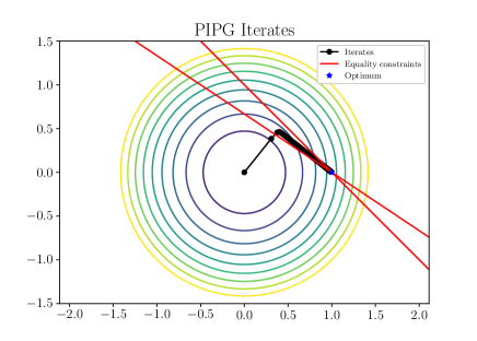
Figure 1: pipg iterates with nearly parallel equality constraints

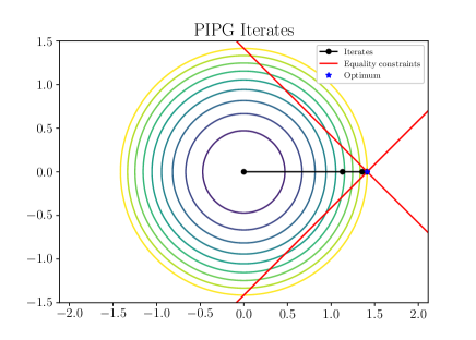
Figure 2: pipg iterates after applying QR preconditioner

We can see that in Figure 1, pipg takes several iterations to converge. Notice that Line 2 of pipg takes a step in the negative gradient direction of the objective function in order to minimize the objective, then takes a step in a direction given by a linear combination of the rows of $H$ (the $H^{\top}w^{k+1}$ term) to satisfy Constraint 1b. The rows of $H$ are the normal vectors of the hyperplanes which define the equality constraints in Problem 1. If we have two equality constraints with nearly parallel hyperplane normals (as in Figure 1), we require smaller coefficients in $w^{k+1}$ for the linear combination of the hyperplane normals, given by $H^{\top}w^{k+1}$, to move the iterates in a direction nearly parallel to hyperplane normals (up and to the right in Figure 1), but require large coefficients for the iterates to move in a direction nearly orthogonal to the hyperplane normals (down and to the right in Figure 1). The coefficients of this linear combination are given by our current iterate of the dual variables $w^{k+1}$. To get large enough $w^{k+1}$ for the iterates to move nearly orthogonal to the hyperplane normals, we must wait for the integrator given by Line 1 to accumulate enough error, resulting in slow convergence.

The QR preconditioner transforms the equality constraints given by Equation 1b to a equivalent set of equality constraints with the same feasible set as the original constraints, but one whose hyperplane normal vectors are all orthogonal and of the same length, making it easy for iterates to move in all directions. After applying the QR preconditioner, we can see the resulting iterates in Figure 2 where the optimum is achieved in far fewer iterations.

IV PARAMETER SELECTION

In this section we will discuss how to select the step-sizes $\alpha$ and $\beta$ to minimize the upper bound on the primal-dual gap for the iterates of pipg.

For convergence of pipg, the primal and dual step-sizes must satisfy the relationship

$$\alpha(\lambda_{\mathrm{max}}+\sigma\beta)<1$$ (6)

where $\alpha$ and $\beta$ are the primal and dual step-sizes respectively, $\lambda_{\mathrm{max}}$ is the maximum eigenvalue of $P$, and $\sigma$ is the maximum eigenvalue of $H^{\top}H$.

There are infinite choices for $\alpha$ and $\beta$ which satisfy the above relationship, and it has been observed that for fastest convergence a “proper” choice for $\alpha$ and $\beta$ must be made. From Proposition 1 of [8], we see that zero primal-dual gap is a sufficient condition for optimality of Problem 1. Thus, we propose to choose step-sizes which minimize the upper bound on the primal-dual gap.

In [10], the authors introduce a positive, scalar parameter, referred to as $\omega$, to select an $\alpha$ and $\beta$ which satisfy the relationship given by Equation 6. We introduce a different scalar parameter $\gamma$, to choose an $\alpha$ and $\beta$ using Equation 2. Using $\gamma$ instead of the previously introduced $\omega$ makes the analysis in this section tractable.

We rewrite Theorem 1 from [8], which provides an upper bound on the primal-dual gap for Algorithm 1 to explicitly show dependence on $\gamma$

$$\mathcal{L}(\bar{z}^{k},w^{\star})-\mathcal{L}(z^{\star},\bar{w}^{k})\leq\frac{f(\gamma)}{k}$$ (7)

$$f(\gamma)=\frac{\lambda_{\mathrm{max}}+\gamma}{2}\|z^{1}-z^{\star}\|^{2}+\frac{\sigma}{2\gamma}\|v^{1}-w^{\star}\|^{2}\\$$ (8)

$$\bar{z}^{k}=\frac{1}{k}\sum_{j=1}^{k}z^{j+1},\;\bar{w}^{k}=\frac{1}{k}\sum_{j=1}^{k}w^{j+1}$$

where $\{z^{j},w^{j}\}_{j=1}^{k}$ are generated by Algorithm 1, $(z^{\star},w^{\star})$ is the optimal primal-dual solution of Problem 1, and $\mathcal{L}(z,w)=\frac{1}{2}z^{\top}Pz+q^{\top}z+w^{\top}(Hz-g)$ is the Lagrangian of Problem 1. Both $\gamma$ and $\sigma$ are defined to be positive real numbers. Under this assumption, we see that $f(\gamma)$ given by Equation 8 is convex in $\gamma$ and has a minimizer given by

$$\gamma^{\star}=\sqrt{\sigma}\frac{\|v^{1}-w^{\star}\|}{\|z^{1}-z^{\star}\|}.$$

Since $\gamma^{\star}$ is a function of the optimal primal-dual solution $(z^{\star},w^{\star})$, we cannot directly choose the optimal step-sizes. Instead, we suggest a heuristic where for every fixed number of iterations of pipg, we pick the value for $\gamma$ which minimizes an approximation of Equation 8, where the optimal primal-dual solution, $(z^{\star},w^{\star})$, is replaced with our current iterates of the primal and dual variables, $(z^{k},w^{k})$. The value of $\gamma$ which minimizes this approximation of Equation 8 after the $k^{th}$ iteration of pipg is

$$\hat{\gamma}^{\star}=\sqrt{\sigma}\frac{\|v^{1}-w^{k}\|}{\|z^{1}-z^{k}\|}.$$

The proposed step-size selection algorithm is given by Algorithm 3. We can combine Algorithms 1, 2, and 3 into Algorithm 4 to show how our proposed algorithms should be used within pipg.

Although choosing $\gamma$ to minimize the upper bound on the primal-dual gap given by Equation 7 only guarantees improving the worst-case performance of pipg, we observe improved convergence in our numerical results.

Algorithm 3 Parameter selection for PIPG

step_selection$z^{1}$, $v^{1}$, $z^{k}$, $w^{k}$, $\lambda_{\mathrm{max}}$, $\sigma$

1:$\hat{\gamma}^{\star}=\sqrt{\sigma}(\|z^{1}-z^{k}\|/\|v^{1}-w^{k}\|)$

2:$\alpha=1/(\lambda_{\mathrm{max}}+\hat{\gamma}^{\star})$

3:$\beta=\hat{\gamma}^{\star}/\sigma$

4:$\alpha$, $\beta$

Algorithm 4 PIPG w/ QR Preconditioner and Parameter Selection

$k_{\max},k_{\mathrm{update}},\alpha_{\mathrm{init}},\beta_{\mathrm{init}},z^{1}\in\mathbb{D},v^{1},H,g$. $z^{k}$.

1:$\hat{H},\hat{g}=\textsc{qr\_preconditioner}(H,g,\lambda_{\mathrm{max}},\lambda_{\mathrm{min}})$

2:$\alpha,\beta=\alpha_{\mathrm{init}},\beta_{\mathrm{init}}$ $k=1,2,\ldots,k_{\max}-1$ $\mathrm{mod}(k,k_{\mathrm{update}})==0$

3:$\alpha,\beta=\textsc{step\_selection}(z^{1},v^{1},z^{k},w^{k},\lambda_{\mathrm{max}},\sigma)$

4:$w^{k+1}=v^{k}+\beta(\hat{H}z^{k}-\hat{g})$

5:$z^{k+1}=\Pi_{\mathbb{D}}[z^{k}-\alpha(Pz^{k}+q+\hat{H}^{\top}w^{k+1})]$

6:$v^{k+1}=w^{k+1}+\beta\hat{H}(z^{k+1}-z^{k})$

V NUMERICAL RESULTS

In this section, we assess the performance of Algorithms 2 and 3 on two MPC problems: regulation of an oscillating mass-spring system and quadrotor obstacle avoidance, a quadratic program (QP) and a second-order cone program (SOCP) respectively. We first define the two problems, discuss implementation details of our algorithms, and finally present the numerical results.

V-A Oscillating Mass Control

The first MPC problem considers regulation of a one-dimensional mass-spring system to equilibrium by applying forces to each of the masses [18]. In this problem there are $N$ masses connected to their neighbors by springs with the masses at the end being connected to a wall with springs.

The state at time-step $t$ is given by $x_{t}=(r_{t},v_{t})$, where $r_{t}\in\mathbb{R}^{N}$ is the displacement of the masses from their respective equilibrium positions, and $v_{t}\in\mathbb{R}^{N}$ is the velocity of the masses. The control at time-step $t$, $u_{t}\in\mathbb{R}^{N}$, is the input forces acting on each of the $N$ masses. We constrain the displacement of the masses (9d), the speed of the masses (9e), and the force applied to each mass (9f). We discretize the dynamics with a zero-order-hold and sample-time of $\Delta t$ and can write the problem as follows

$$\underset{x_{t},u_{t}}{\mathrm{minimize}}\quad \frac{1}{2}\left(\sum_{t=1}^{T}x_{t}^{\top}Q_{t}x_{t}+\sum_{t=1}^{T-1}u_{t}^{\top}R_{t}u_{t}\right)$$ (9a)

$$\mathrm{subject\;to}\quad x_{t+1}=Ax_{t}+Bu_{t}\;\quad t\in[1,T-1]$$ (9b)

$$x_{1}=x_{\mathrm{init}}$$ (9c)

$$\|r_{t}\|_{\infty}\leq r_{\mathrm{max}}\quad\quad\quad\quad\!\!\!t\in[1,T]$$ (9d)

$$\|v_{t}\|_{\infty}\leq v_{\mathrm{max}}\quad\quad\quad\quad\!\!\!t\in[1,T]$$ (9e)

$$\|u_{t}\|_{\infty}\leq u_{\mathrm{max}}\quad\quad\quad\quad\!\!\!\!t\in[1,T-1].$$ (9f)

All the masses have unit mass, all the springs have unit spring constant, the following non-dimensional parameters are used,

$$\begin{split}T&=30,\;\Delta t=0.1,\;N=8,\;\\ r_{\mathrm{max}}&=0.75,\;v_{\mathrm{max}}=0.75,\;u_{\mathrm{max}}=0.5\\ Q_{t}&=\mathrm{blkdiag}(I_{N},5I_{N}),\;R_{t}=I_{N}.\end{split}$$

Each component of the initial state $x_{\mathrm{init}}$ is drawn from the uniform distribution on the interval [-0.5, 0.5].

The dynamics given by Equation 9b can be written as Constraint 1b with appropriate choice of $H$ and $g$. Constraints 9d, 9e, and 9f can be written as Constraint 1c, where $\mathbb{D}$ is the Cartesian product of boxes.

V-B Quadrotor Path Planning

The second MPC problem considered is the three-degree-of-freedom quadrotor path planning problem with obstacle avoidance. The state at time-step $t$ is defined as $x_{t}=(r_{t},v_{t})$, where $r_{t}\in\mathbb{R}^{3}$ is the position of the quadrotor, and $v_{t}\in\mathbb{R}^{3}$ is the velocity of the quadrotor. The control at time $t$, $u_{t}\in\mathbb{R}^{3}$, is the thrust produced by the quadrotor’s propellers.

Unlike the oscillating masses regulation problem, where the goal is to regulate all the masses to their equilibrium positions, the objective in this problem is to track a reference trajectory given by $\hat{x}_{t}$ which linearly interpolates the initial state $x_{\mathrm{init}}$ and the desired target state $x_{\mathrm{target}}$. However, this reference trajectory intersects the obstacle, forcing the optimizer to compute a trajectory that avoids that obstacle. The dynamics of this system are given by a double integrator in three dimensions subject to gravity. These dynamics are discretized with a zero-order-hold to obtain the discrete-time linear system given by 10b, where

$$A=\begin{bmatrix}I_{3}&(\Delta t)I_{3}\\ 0_{3}&I_{3}\end{bmatrix}\hskip 7.11317pt$$

$$B=\frac{1}{m}\begin{bmatrix}(1/2)(\Delta t)^{2}I_{3}\\ (\Delta t)I_{3}\end{bmatrix}$$

$$c=\begin{bmatrix}0_{2\times 1}\\ -(1/2)g(\Delta t)^{2}\\ 0_{2\times 1}\\ -g(\Delta t)\end{bmatrix}$$

$g=9.8$ is the non-dimensional gravitational acceleration and $m$ is the mass of the quadrotor.

We impose two control constraints: an upper bound on thrust (10f) and a thrust pointing constraint (10g). The thrust pointing constraint is a proxy to constrain the tilt angle of the quadrotor, since we are using a three-degree-of-freedom model and cannot directly constrain the quadrotor’s tilt.

A cylindrical keep-out zone can be written as

$$\|r_{t}^{1:2}-r_{c}\|_{2}\geq\rho$$

where $r_{c}$ is the position of the center of the obstacle and $\rho$ is the radius of the obstacle. This constraint, however, is nonconvex.

This nonconvex keep-out-zone constraint can be replaced with a convex rotating half-space constraint, as in [9]. This rotating half-space constraint is written as 10d with

$$\begin{split}a_{t}&=[\cos(\psi t+\phi)\;-\sin(\psi t+\phi)]^{\top}\\ b_{t}&=-a_{t}^{\top}r_{c}-\rho\end{split}$$

where $\psi$ is the rotation rate of the half-space and $\phi$ is the initial phase offset of the half-space. This problem can be written as

$$\underset{x_{t},u_{t}}{\mathrm{minimize}}~{} \frac{1}{2}\left(\sum_{t=1}^{T}(x_{t}-\hat{x}_{t})^{\top}Q_{t}(x_{t}-\hat{x}_{t})\right.$$ (10a)

$$\left.\quad+\sum_{t=1}^{T-1}u_{t}^{\top}R_{t}u_{t}\right)$$

$$\mathrm{subject~{}to}~{} x_{t+1}=Ax_{t}+Bu_{t}+c \!\!\!\!\!\!\!\!\!\!\!\!\!\!\!t\in[1,T-1]$$ (10b)

$$x_{1}=x_{\mathrm{init}}$$ (10c)

$$a_{t}^{\top}r_{t}\leq b_{t} \!\!\!\!\!\!\!\!\!\!\!\!\!\!\!t\in[1,T]$$ (10d)

$$\|v_{t}\|_{2}\leq v_{\mathrm{max}} \!\!\!\!\!\!\!\!\!\!\!\!\!\!\!t\in[1,T]$$ (10e)

$$\|u_{t}\|_{2}\leq u_{\mathrm{max}} \!\!\!\!\!\!\!\!\!\!\!\!\!\!\!t\in[1,T-1]$$ (10f)

$$\cos(\theta_{\mathrm{max}})\|u_{t}\|_{2}\leq u_{t}^{\top}e \!\!\!\!\!\!\!\!\!\!\!\!\!\!\!t\in[1,T-1]$$ (10g)

where $e=[0\;0\;1]^{\top}$. Additionally, the following non-dimensional parameters are used

$$\begin{split}T&=30,\;\Delta t=0.2,\;m=3,\;\psi=-0.5\\ \phi&=-\pi/4,\;r_{c}=[2.5\;2.5]^{\top},\;\rho=0.25\\ v_{\mathrm{max}}&=1.5,\;u_{\mathrm{max}}=35,\;\theta_{\mathrm{max}}=0.1745\\ Q_{t}&=\mathrm{blkdiag}(2I_{3},I_{3}),\;R_{t}=0.5I_{3}\\ x_{\mathrm{init}}&=[0\;0\;5\;0\;0\;0],\;x_{\mathrm{target}}=[5\;5\;5\;0\;0\;0].\end{split}$$

With proper choice for $H$ and $g$, we can rewrite the dynamics given by Constraint 10b in the form of Constraint 1b. Constraint 10d represents a half-space, Constraint 10e represents a ball, and Constraints 10f and 10g represent the intersection of a ball and a second-order cone. We can write all of these constraints as Constraint 1c, where $\mathbb{D}$ is the Cartesian product of the aforementioned sets.

V-C Implementation Details

We generate our numerical results using MATLAB. From Algorithm 2, we determine that the maximum eigenvalue of $H^{\top}H$ is $\eta^{2}$. If Algorithm 2 is not used, we use power iteration to compute the maximum eigenvalue of $H^{\top}H$ [16]. To compute maximum and minimum eigenvalues of $P$, $\lambda_{\mathrm{max}}$ and $\lambda_{\mathrm{min}}$ respectively, we simply take the maximum and minimum diagonal elements of $P$ since $P$ is diagonal in our examples. For general $P\succ 0$, we can compute the maximum eigenvalue with power iteration and minimum eigenvalue with either shifted power iteration or inverse power iteration. In all examples, we use $k_{\mathrm{update}}=25$ when testing Algorithm 3. When running examples without using Algorithm 3, we set $\gamma=\sigma$ which makes the dual step-size $\beta=1$ consistent with the implementation in [8]. We run the oscillating-mass problem $50$ times with $50$ different initial conditions drawn from the distribution described in the previous section.

Figures 3 and 4 depict the sparsity pattern of $H$ for MPC problems before and after applying the QR preconditioner. Applying the preconditioner results in significant fill-in, i.e., the introduction of nonzero elements in a sparse matrix where they did not exist previously. In the pipg implementation, $H$ is stored as a sparse matrix when the QR preconditioner is not applied, but $H$ is stored as a dense matrix when the preconditioner is applied. This choice of data structure results in faster matrix-vector multiplication for each case. Without preconditioning, the percentage of nonzero elements in $H$ is small enough that sparse matrix vector multiplication is faster than dense matrix vector multiplication. However, after applying the QR preconditioner, $H$ contains too high of a percentage of nonzero elements for sparse matrix-vector multiplication to be faster than dense matrix-vector multiplication. Consequently, the QR preconditioner is limited to problems and embedded systems where the extra storage requirement for the preconditioned, dense $H$ matrix is not restrictive. Before preconditioning, when we store $H$ for both problems in compressed sparse column (CSC), it takes roughly 187 kilobytes for the oscillating masses problem and 11.6 kilobytes for the quadrotor problem. After applying our preconditioner and storing the preconditioned matrix as a dense matrix, it takes roughly 2581 kilobytes for the oscillating masses problem and 363 kilobytes of storage for the quadrotor problem. As the problem size increases, the storage requirements for the dense matrix become more demanding.

Figure 3: Sparsity plot of $H$ for the oscillating mass problem

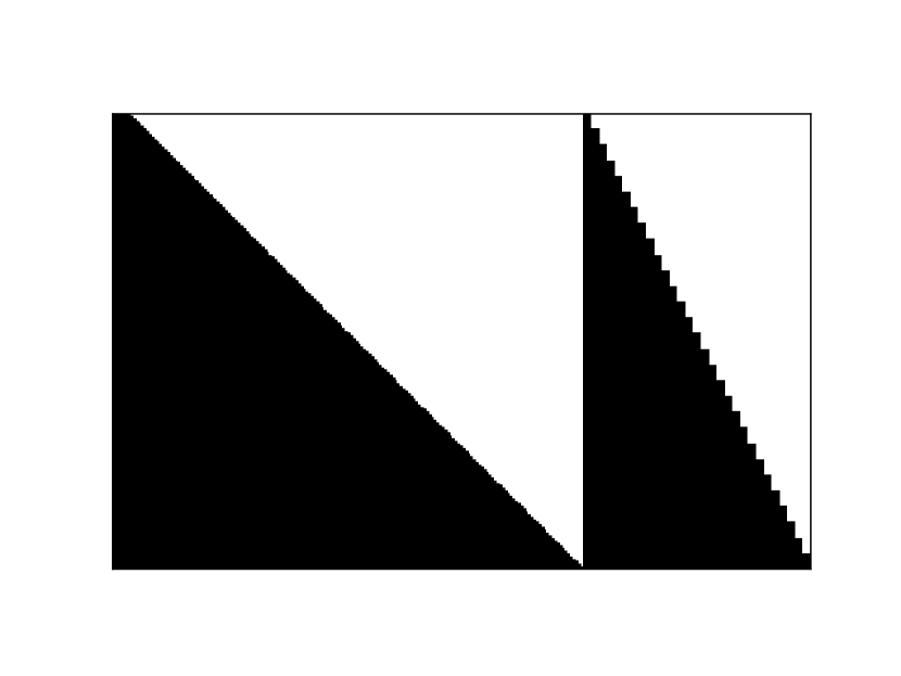
Figure 4: Sparsity plot of $\hat{H}$ for the oscillating mass problem

V-D Analysis of results

We assess the effect of the our algorithms using two metrics: relative distance to optimum and feasibility as defined below

$$\mathrm{error}_{\mathrm{opt}}=\frac{\|z^{k}-z^{\star}\|_{\infty}}{\|z^{\star}\|_{\infty}},\;\mathrm{error}_{\mathrm{feas}}=\frac{\|Hz^{k}-g\|_{\infty}}{\|z^{\star}\|_{\infty}}$$

where $z^{\star}$ is the solution to 1 computed by Gurobi [19] using YALMIP [20]. We terminate pipg when the relative error, $\mathrm{error}_{\mathrm{opt}}$, decreases below $1.0\times 10^{-4}$, indicating the solution has a relative error of $0.01\%$.

For the oscillating masses problem, we test the QR preconditioner against modified Ruiz equilibration. For this problem, modified Ruiz equilibration preserves closed-form projection onto set $\mathbb{D}$ since set $\mathbb{D}$ is a box before and after transformation. Additionally, we test the hypersphere preconditioner (HS) on the quadrotor problem, since in this case, the transformed set $\mathbb{D}$ still has a closed-form projection. If our state cost matrix $Q_{t}$ penalized each component of velocity by different weights or the control cost matrix $R_{t}$ penalized each component of thrust with different weights, the HS preconditioner will induce a change of variables which will result in the transformed set $\mathbb{D}$ containing ellipsoids and no longer having closed-forms projections. The hypersphere preconditioner involves multiplying the preconditioned cost function by some $\lambda>0$ similar to how the QR preconditioner multiplies the equality constraints by some $\eta>0$, however the authors do not provide a way of selecting this $\lambda$ [7]. In our numerical results, we choose the $\lambda$ for the hypersphere preconditioner such that the condition number of the KKT matrix given by Equation 4 is minimized.

Figure 5 depicts the distribution of the absolute value of the eigenvalues for the KKT matrix of the oscillating masses problem and quadrotor problem before and after applying the QR preconditioner. Applying the preconditioner shrinks the interval on which the eigenvalues are distributed, making the maximum and minimum eigenvalues closer in magnitude to each other, reducing the condition number of the KKT matrix.

Figures 6 and 7 show that the QR preconditioner and the step-size heuristic cause pipg to converge in fewer iterations when applied independently. When applied together, we observed a further reduction in iteration count. Applying the QR preconditioner also results in fewer iterations to convergence than applying modified Ruiz equilibration or the hypersphere preconditioner. Note that for the oscillating-mass problem, pipg without step-selection and the QR preconditioner requires many more than $1500$ iterations to meet our stopping criteria, but we only plotted the first $1500$ iterations for clarity.

Tables I and II contain the solve-times for our numerical examples. The solve-times in the table do not include preconditioning time for any of the preconditioners, since for MPC problems we can perform the preconditioning offline and only have to incur cost of solving the preconditioned problem. We observe that the time to perform the QR preconditioning was very small for the problems we considered: $11.9$ and $1.75$ milliseconds for the oscillating masses problem and quadrotor problem respectively. Our two proposed algorithms result in solve-time reductions, and we see that the QR preconditioner is more effective at reducing solve-times than modified Ruiz equilibration and the hypersphere preconditioner.

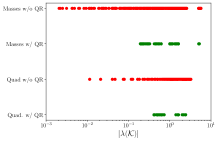
Figure 5: Eigenvalue distribution of the KKT matrix for the oscillating masses and quadrotor problems with and without applying the QR preconditioner

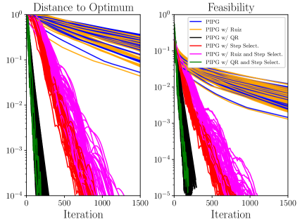
Figure 6: $\mathrm{error}_{\mathrm{opt}}$ (left) and $\mathrm{error}_{\mathrm{feas}}$ (right) for the oscillating masses problem

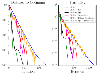
Figure 7: $\mathrm{error}_{\mathrm{opt}}$ (left) and $\mathrm{error}_{\mathrm{feas}}$ (right) for the quadrotor problem

	Without Precond.	With Ruiz	With QR
Without Step Select.	651.73	562.80	23.96
With Step Select.	50.85	60.71	18.69

TABLE I: Average solve-time in milliseconds over 50 runs for the oscillating masses problem

	Without Precond.	With HS	With QR
Without Step Select.	226.92	169.50	93.68
With Step Select.	114.91	91.80	62.04

TABLE II: Average solve-time in milliseconds over 100 runs for the quadcopter problem

VI CONCLUSION

We develop the QR preconditioner to speed up pipg, a first-order primal-dual algorithm, by applying a transformation to equality constraints which minimizes the condition number of the KKT matrix for the optimization problem. We then introduce a step-size heuristic for pipg based on minimizing the upper bound on the primal-dual gap. The effectiveness of these algorithms are demonstrated on two MPC problems, where we provide comparisons to existing preconditioning algorithms.

References

- [1] Heinz H. Bauschke and Patrick L. Combettes. Convex analysis and monotone operator theory in hilbert spaces. In CMS Books in Mathematics, 2011.
- [2] Heinz H. Bauschke, Minh N. Bui, and Xianfu Wang. Projecting onto the intersection of a cone and a sphere. SIAM Journal on Optimization, 28(3):2158–2188, 2018.
- [3] Juan L. Jerez, Paul J. Goulart, Stefan Richter, George A. Constantinides, Eric C. Kerrigan, and Manfred Morari. Embedded online optimization for model predictive control at megahertz rates. IEEE Transactions on Automatic Control, 59(12):3238–3251, 2014.
- [4] Goran Banjac, Bartolomeo Stellato, Nicholas Moehle, Paul Goulart, Alberto Bemporad, and Stephen Boyd. Embedded code generation using the osqp solver. In 2017 IEEE 56th Annual Conference on Decision and Control (CDC), pages 1906–1911, 2017.
- [5] Euhanna Ghadimi, André Teixeira, Iman Shames, and Mikael Johansson. Optimal parameter selection for the alternating direction method of multipliers (admm): Quadratic problems. IEEE Transactions on Automatic Control, 60(3):644–658, 2015.
- [6] B. Stellato, G. Banjac, P. Goulart, A. Bemporad, and S. Boyd. OSQP: an operator splitting solver for quadratic programs. Mathematical Programming Computation, 12(4):637–672, 2020.
- [7] Abhinav G Kamath, Purnanand Elango, Taewan Kim, Skye Mceowen, Yue Yu, John M Carson III, Mehran Mesbahi, and Behçet Açıkmeşe. Customized real-time first-order methods for onboard dual quaternion-based 6-dof powered-descent guidance. In AIAA SciTech 2023 Forum, 2023.
- [8] Yue Yu, Purnanand Elango, Ufuk Topcu, and Behçet Açıkmeşe. Proportional–integral projected gradient method for conic optimization. Automatica, 142:110359, 2022.
- [9] Yue Yu, Purnanand Elango, and Behçet Açıkmeşe. Proportional-integral projected gradient method for model predictive control. IEEE Control Systems Letters, 5(6):2174–2179, 2021.
- [10] Yue Yu, Purnanand Elango, Behçet Açıkmeşe, and Ufuk Topcu. Extrapolated proportional-integral projected gradient method for conic optimization. IEEE Control Systems Letters, 7:73–78, 2023.
- [11] Purnanand Elango, Abhinav G Kamath, Yue Yu, John M Carson III, Mehran Mesbahi, and Behçet Açıkmeşe. A customized first-order solver for real-time powered-descent guidance. In AIAA SciTech 2022 Forum, page 0951, 2022.
- [12] Abhinav G. Kamath, Purnanand Elango, Yue Yu, Skye Mceowen, Govind M. Chari, John M. Carson III, and Behçet Açıkmeşe. Real-time sequential conic optimization for multi-phase rocket landing guidance. IFAC-PapersOnLine, 56(2):3118–3125, 2023. 22nd IFAC World Congress.
- [13] Govind M. Chari, Abhinav G. Kamath, Purnanand Elango, and Behcet Acikmese. Fast monte carlo analysis for 6-dof powered-descent guidance via gpu-accelerated sequential convex programming. In AIAA SciTech 2024 Forum, 2024.
- [14] Govind M Chari and Behçet Açıkmeşe. Spacecraft rendezvous guidance via factorization-free sequential convex programming using a first-order method. arXiv preprint arXiv:2402.04561, 2024.
- [15] Michele Benzi, Gene H. Golub, and Jörg Liesen. Numerical solution of saddle point problems. Acta Numerica, 14:1–137, 2005.
- [16] Gene H Golub and Charles F Van Loan. Matrix Computations. Johns Hopkins Series in the Mathematical Sciences. Johns Hopkins University Press, Baltimore, MD, 3 edition, October 1996.
- [17] Jorge Nocedal and Stephen Wright. Numerical Optimization. Springer Series in Operations Research and Financial Engineering. Springer, New York, NY, 2 edition, July 2006.
- [18] Yang Wang and Stephen Boyd. Fast model predictive control using online optimization. IEEE Transactions on Control Systems Technology, 18(2):267–278, 2010.
- [19] Gurobi Optimization, LLC. Gurobi Optimizer Reference Manual, 2023.
- [20] J. Löfberg. Yalmip : A toolbox for modeling and optimization in matlab. In In Proceedings of the CACSD Conference, Taipei, Taiwan, 2004.