The Effectiveness of Local Updates for Decentralized Learning under Data Heterogeneity

Abstract

We revisit two fundamental decentralized optimization methods, Decentralized Gradient Tracking (DGT) and Decentralized Gradient Descent (DGD), with multiple local updates. We consider two settings and demonstrate that incorporating $K>1$ local update steps can reduce communication complexity. Specifically, for $\mu$-strongly convex and $L$-smooth loss functions, we proved that local DGT achieves communication complexity $\tilde{\mathcal{O}}\Big{(}\frac{L}{\mu K}+\frac{\delta}{\mu(1-\rho)}+\frac{\rho}{(1-\rho)^{2}}\cdot\frac{L+\delta}{\mu}\Big{)}$, where $\rho$ measures the network connectivity and $\delta$ measures the second-order heterogeneity of the local loss. Our result reveals the tradeoff between communication and computation and shows increasing $K$ can effectively reduce communication costs when the data heterogeneity is low and the network is well-connected. We then consider the over-parameterization regime where the local losses share the same minimums, we proved that employing local updates in DGD, even without gradient correction, can yield a similar effect as DGT in reducing communication complexity. Numerical experiments validate our theoretical results.

I Introduction

We consider a network of $m$ agents collaboratively solving the following deterministic finite sum minimization problem:

$$\underset{\bm{x}\in\mathbb{R}^{d}}{\min}~{}\left\{f(\bm{x}):=\frac{1}{m}\sum_{i=1}^{m}{f_{i}(\bm{x})}\right\},$$ (1)

where $\bm{x}\in\mathbb{R}^{d}$ is the decision variable shared by all agents, each $f_{i}:\mathbb{R}^{d}\to\mathbb{R}$ is the local loss function private to agent $i$. The average loss $f$ is assumed to be $L$-smooth. The agents are allowed to communicate with each other via a fixed network. Problem (1) has found applications in many areas, including machine learning, signal processing, telecommunications, finance, multi-agent control,etc.[1, 2, 3, 4].

Algorithms for solving (1) have been intensively studied in the literature [5]. By collaboratively learning over the network, these algorithms aim to benefit from aggregating the resources (computation and samples) of multiple agents and attain improved training efficiency and model precision. However, due to decentralization, achieving such a goal comes at the cost of communication resources, which usually becomes the bottleneck of the algorithm for large-scale problems. Designing algorithms with reduced communication costs without sacrificing learning performance is therefore of paramount importance.

Among methods developed to improve communication efficiency, a well-known approach is to perform multiple local computation steps before communicating with network neighbors. The idea serves as the basis of the local SGD algorithm [6] and has been employed as a standard practice for algorithm design in both federated learning (FL) and decentralized settings with a mesh network. Running multiple local gradient steps accelerates the optimization process. However, when the $f_{i}$s have heterogeneous gradients, modifying algorithms by naively increasing the number of local updates may introduce client drift, leading to non-convergence with a constant step size [7, 8, 9]. As a remedy, variance reduction (VR)/gradient tracking (GT) techniques are often employed to correct such bias. The idea leads to the renowned DGT algorithm with exact convergence [10, 11, 12]. Along this line, a fundamental question to understand is:

Will increasing local computations be beneficial in reducing the communication overhead?

Furthermore, since these methods eliminate the impact of gradient heterogeneity on the convergence, it is interesting to understand:

If, and to what degree, will the difference in the $f_{i}$s affect the computation-communication tradeoff?

Apart from the classical setting where each loss function admits different minimizers, modern learning tasks often employ models with a large number of parameters. This leads to the over-parameterization regime with the models learned perfectly interpolating the training data [13, 14]. In this setting, problem (1) enjoys the property that all the $f_{i}$s have at least one common minimizer, implying that the gradient heterogeneity vanishes at these optimums. This motivates us to revisit the two questions above for the DGD algorithm without bias correction, which still achieves exact convergence [15].

Common to all these scenarios, the algorithms either do not suffer from or actively eliminate the impact of gradient (first-order) heterogeneity on the convergence. A natural conjecture is that under these cases, the difference in the second-order derivatives of the $f_{i}$s will be a dominating factor affecting the convergence rate. This is the central question we investigate in this work.

I-A Summary of contributions

In this paper, we study the above questions for the DGD and DGT algorithms, whose vanilla versions perform only one gradient update followed by network communication. We consider two settings: (i) when the average loss $f$ is $\mu$-strongly convex or satisfies the Polyak-Łojasiewicz (PL) condition, and (ii) the over-parameterization regime where $f$ is PL and $\beta$-weakly convex, and all the $f_{i}$s share at least one minimizer. Our contributions are:
$\bullet$ In setting (i) with strongly convex $f$, we proved Local DGT (DGT with properly incorporated local computations) converges to an $\varepsilon$-optimal solution linearly with communication complexity $\tilde{\mathcal{O}}\Big{(}\frac{L}{\mu K}+\frac{\delta}{\mu(1-\rho)}+\frac{\rho}{(1-\rho)^{2}}\cdot\frac{L+\delta}{\mu}\Big{)}$, where $\rho$ measures the network connectivity, $K$ is the number of local updates per communication round, and $\delta$ measures the second-order heterogeneity of the $f_{i}$s (cf. Assumption 3). Our result reveals when the heterogeneity degree $\delta$ is small and the network is well-connected, increasing local updates $K$ can significantly reduce communication overhead. The result is further generalized for PL objectives.
$\bullet$ In setting (ii), we proved when the degree of heterogeneity is small such that $\zeta:=1-(\delta/\mu)^{2}\in(0,1)$, local DGD converges linearly with communication complexity $\tilde{\mathcal{O}}\left(\frac{L}{\mu Kr}+\frac{1}{1-\rho}+\frac{\beta+\rho^{2}L}{\mu(1-\rho)^{2}r^{2}}\right)$. As such, increasing local updates is effective when $f$ is (near)-convex and the network is well-connected.
$\bullet$ We further improved the result for setting (ii) under the linear regression model. For arbitrary bound $\delta$, it takes local DGD $\tilde{\mathcal{O}}\left(\frac{L}{\mu K}+\frac{\delta^{2}}{\mu^{2}(1-\rho)}\right)$ communication rounds to reach the minimizer with minimum $\ell_{2}$-norm, where $\mu$ and $L$ are respectively the smallest and largest nonzero eigenvalue of the design covariance matrix.

I-B Related works

In recent years, the design and analysis of federated/decentralized learning algorithms have been extensively explored in different settings. Many of them aim to show the algorithm of interest is convergent when employing multiple local computation steps. In the stochastic setting, there are some related works proving performing local updates can reduce the algorithms’ steady state error related to the gradient sampling variance, we refer the readers to the expression of these convergence rates reported in [9, 16, 8, 17]. Essentially, such a speed up is due to the reduction of variance when averaging independent stochastic gradients both across the iterations and the network agents. A majority of them, however, cannot show the benefit of local updates to the transient terms. The drawback is two-fold. First, when particularized to the deterministic setting, they fail to answer the important algorithm design question of if applying local updates can accelerate communication. Second, in the stochastic setting, they cannot show algorithms of local SGD type is more communication efficient than the simple minibatch SGD baseline [7, 8, 16]. In the following, we review and contrast our results to those managed to show local updates are beneficial in reducing the communication complexity either in the deterministic setting or transient terms in the stochastic setting, which are far less.

In the FL setting where a center node is connected to and coordinates all worker nodes, local GD [6] has been among the most popular algorithms employing local updates in between communication rounds. In the presence of gradient heterogeneity, it is known that local GD and its variations cannot achieve exact convergence with a constant step size due to “client drift” [18, 8]. With a diminishing step size, [8] is the first to show local SGD improves over minibatch SGD with each $f_{i}$ being convex. To mitigate the impact of gradient heterogeneity, VR and primal-dual-based methods correct the gradient direction, leading to exact convergence with constant step size, see e.g. [18, 19, 16]. Provable benefit of performing multiple local updates while guaranteeing the exact convergence is established only in restricted settings, such as requiring each $f_{i}$ to be strongly convex and smooth  [16] or quadratic [18]. Our result when particularized to the FL setting, incorporates a larger family of problems and recovers/improves existing results, see discussions in Sec. III-A1.

In the decentralized setting with a mesh communication network, it is known that even the vanilla DGD algorithm suffers from non-convergence under gradient heterogeneity [20]. Despite being standard techniques to overcome the issue, algorithms employing gradient correction techniques with proactively designed communication-computation pattern is discussed in only a few recent works [16, 21, 17, 22, 23, 24]. These results show that in the stochastic setting, increasing local updates can reduce the steady-state stochastic error but not the transient terms. The only exception we are aware of is Scaffnew [16], which shows provable benefit assuming each $f_{i}$ is strongly convex and smooth.

When it comes to overparameterized objective functions, the performance of DGD has been studied in [9, 15]. Exact linear convergence is shown in [9] assuming each $f_{i}$ is strongly convex, with communication complexity $\tilde{\mathcal{O}}\left(\frac{L}{\mu(1-\rho)}\right)$. The result is further improved to $\tilde{\mathcal{O}}\left(\frac{L}{\mu K}\right)$ in [15] under the same condition, showing network-independent complexity. However, it is worth noting that in this case all $f_{i}$s will share a same unique minimizer, implying that the agents can just solve their local problems independently without the network. On the contrary, we analyzed the convergence under a more general PL condition on the average loss $f$, but allowing the local $f_{i}$s to have different sets of minimizers. Consequently, our problem structure is fundamentally different from [9] and  [15], and network communication is necessary to find a consensus solution.

Finally we note that there exist works considering distributed optimization in solving special instances of overparameterized problems. For example, a compression-based algorithm was proposed in [25], achieving problem dimension-independent communication complexity. A communication-efficient distributed algorithm was developed in [26] for a class of overparameterized kernel learning. Linear convergence of local GD/SGD for specific overparameterized neural networks has been established in [27, 28]. These results are complementary to ours, as they either study under special problem structures, propose new methods, or prove convergence without considering the effectiveness of local updates. In contrast, we aim to understand the performance guarantees of the arguably most widely used distributed algorithms: DGD and DGT with local updates.

Notations. We use lowercase bold letters (e.g., $\bm{x},\bm{y}$) and capital bold letters (e.g., $\bm{A},\bm{B}$) to denote vectors and matrices, respectively. $\|\cdot\|$ and $\|\cdot\|_{2}$ respectively denotes the Frobenius norm and spectral norm (maximum singular value) of a matrix. Denote $[m]\triangleq\{1,2,\cdots,m\}$ and $\bm{I}_{m}\in\mathbb{R}^{m\times m}$ is the identity matrix. We write $a_{n}\lesssim b_{n}$ if there exists a universal constant $C$ such that $a_{n}\leq Cb_{n}$ and $a_{n}=\mathcal{O}(b_{n})$ have the same meaning. Moreover, $a_{n}=\tilde{\mathcal{O}}(b_{n})$ means $a_{n}\leq Cb_{n}$ up to some polylogarithmic factors.

II Preliminaries: DGD/DGT with local updates

We consider solving problem (1) over a mesh network modeled as an undirected graph $\mathcal{G}:=\{\mathcal{V},\mathcal{E}\}$, with nodes $\mathcal{V}:=\{1,\ldots,m\}$ representing the set of agents and edges $\mathcal{E}\subseteq\mathcal{V}\times\mathcal{V}$ representing the communication links. An unordered pair $\{i,j\}\in\mathcal{E}$ if and only if there is a bi-directional communication channel between them. The one-hop neighbors of agent $i$ is denoted by $\mathcal{N}_{i}:=\{j\in\mathcal{V}\,|\,\{i,j\}\in\mathcal{E}\}$.

Given problem (1), the local DGD algorithm optimizes parameter $\bm{x}$ by alternating two steps: (1) local optimization where each agent $i$ updates its local model $\bm{x}_{i}$ by performing $K$ gradient descent steps; (2) network communication where each agent $i$ aggregates information from their network neighbors by averaging the model parameters following a gossip consensus communication protocol [29]. Formally, let $\bm{x}^{i}$ denote the local model of agent $i$. In each communication round $r$, agent $i$ performs:

$$\begin{split}\bm{x}_{r,k+1}^{i}&=\bm{x}_{r,k}^{i}-\eta\nabla f_{i}(\bm{x}_{r,k}^{i}),\ \forall k=0,\ldots,K-1,\\ \bm{x}_{r+1,0}^{i}&=\sum_{j\in\mathcal{N}_{i}}w_{ij}\left(\bm{x}_{r,K}^{j}-\eta\nabla f_{j}(\bm{x}_{r,K}^{j})\right),\end{split}$$ (2)

where $\eta>0$ is a prescribed step size, and $\{w_{ij}\}_{i=1}^{m}$ are weights employed to force the consensus of the $\bm{x}^{i}$s. Note that when $w_{ij}=1/m$, the local DGD algorithm reduces to FedAvg (local GD) [6].

It is well recognized that when the $f_{i}$’s are heterogeneous, even the vanilla DGD algorithm cannot converge to the exact solution due to the gradient heterogeneity, i.e., $\sum_{i=1}^{m}\|\nabla f_{i}(\bm{x})-\nabla f(\bm{x})\|>0$ [20, 30]. As a remedy, the gradient tracking technique [11, 12, 10] is employed to correct the direction and achieve exact convergence. When incorporating multiple local updates, the local DGT algorithm is developed in [21, 17]. Specifically, in each communication round $r$, agent $i$ performs:

$$\begin{split}\bm{x}_{r,k+1}^{i}&=\bm{x}_{r,k}^{i}-\eta\bm{y}_{r,k}^{i}\\ \bm{y}^{i}_{r,k+1}&=\bm{y}^{i}_{r,k}+\nabla f_{i}(\bm{x}^{i}_{r,k+1})-\nabla f_{i}(\bm{x}^{i}_{r,k})\end{split}$$ (3)

for $k=0,\ldots,K-1$ while averages in the last step:

$$\bm{x}^{i}_{r+1,0} =\sum_{j\in\mathcal{N}_{i}}{w_{ij}\left(\bm{x}^{j}_{r,K}-\eta\bm{y}^{j}_{r,K}\right)}$$ (4)

$$\bm{y}^{i}_{r+1,0} =\sum_{j\in\mathcal{N}_{i}}{w_{ij}\left(\bm{y}^{j}_{r,K}+\nabla f_{j}(\bm{x}^{j}_{r+1,0})-\nabla f_{j}(\bm{x}^{j}_{r,K})\right)}.$$

The auxiliary variable $\bm{y}^{i}$ is the tracking variable introduced as an estimator of the average gradient $\nabla f(\bm{x}^{i})$, initialized as $\bm{y}_{0,0}^{i}=\nabla f_{i}(\bm{x}_{0,0}^{i})$.

In this paper, we consider the impact of local updates on the communication-computation tradeoffs and its effectiveness in reducing communication costs, for the above two algorithms applied to the problem (1) under the following standard assumptions.

Assumption 1.

The average loss function $f:\mathbb{R}^{d}\to\mathbb{R}$ is $L$-smooth, i.e., for all $\bm{x},\bm{y}\in\mathbb{R}^{d}$ it holds

$$\|\nabla f(\bm{x})-\nabla f(\bm{y})\|\leq L\|\bm{x}-\bm{y}\|.$$ (5)

Assumption 2.

The communication network $\mathcal{G}$ is connected. The weight matrix $\bm{W}=[w_{ij}]_{ij=1}^{m}$ of graph $\mathcal{G}$ satisfies (i) $w_{ij}=0$ for all $\{i,j\}\notin\mathcal{E}$; (ii) doubly stochastic: $\mathbf{1}^{T}_{m}\bm{W}=\mathbf{1}^{T}_{m}$ and $\bm{W}\mathbf{1}_{m}=\mathbf{1}_{m}$; (iii) and $\rho:=\left\|\bm{W}-(1/m)\bm{1}_{m}\bm{1}_{m}^{T}\right\|_{2}<1$.

We further assume the $f_{i}$s have bounded second-order heterogeneity, as given by Assumption 3.

Assumption 3.

Each $f_{i}$ is $C^{1}$ and satisfies for all $\bm{x},\bm{y}\in\mathbb{R}^{d}$ and $i\in[m]$:

$$\|\nabla f(\bm{x})-\nabla f_{i}(\bm{x})-(\nabla f(\bm{y})-\nabla f_{i}(\bm{y}))\|^{2}\leq\delta^{2}\|\bm{x}-\bm{y}\|^{2}.$$ (6)

Note that when the $f_{i}$s are second order continuously differentiable, Assumption 3 can be implied by the following bound on Hessian similarity:

$$\|\nabla^{2}f(\bm{x})-\nabla^{2}f_{i}(\bm{x})\|\leq\delta;\quad\forall\bm{x}\in\mathbb{R}^{d},\,\forall i\in[m].$$ (7)

III Main results

This section studies the communication-computation tradeoffs of the local DGD and DGT algorithms. We first consider the setting where the average loss function $f$ is strongly convex. The communication complexity of local DGT is presented in Section III-A. The result is further generalized for weakly convex $f$ satisfying the PL condition. Then we consider over-parameterized problems where the local $f_{i}$s have at least one common minimizer. The communication complexity of local DGD is provided in Section III-B. In both cases, our result shows the communication-computation tradeoff is affected by the second-order heterogeneity of the $f_{i}$s.

III-A Local DGT under strong convexity

Assumption 4.

The average loss function $f$ is $\mu$-strongly convex, i.e., for all $\bm{x},\bm{y}\in\mathbb{R}^{d}:$

$$f(\bm{y})\geq f(\bm{x})+\langle\nabla f(\bm{x}),\bm{y}-\bm{x}\rangle+\frac{\mu}{2}\|\bm{y}-\bm{x}\|^{2}.$$ (8)

To state the convergence, we introduce the following potential function that measures the optimality gap at the end of round $R$:

$$P^{R}:=\mu\Big{(}f(\overline{\bm{x}}^{R+1})-f^{\star}\Big{)}\\ +\frac{1}{\sum_{r=0}^{R}{w_{r}}}\sum_{r=0}^{R}{\Bigg{(}\frac{w_{r}\sum_{i=1}^{m}\!{\sum_{k=0}^{K}{\|\nabla f(\bm{x}^{i}_{r,k})\|^{2}}}}{m(K+1)}\Bigg{)}},$$ (9)

where $f^{\star}$ denotes the minimum of $f$ and $\{w_{r}\}$ is an increasing geometric sequence whose formula is given in the proof.

Theorem 1.

(strong convexity). Consider problem (1) with the average loss $f$ satisfying Assumption 1 and 4. Suppose the $f_{i}$s satisfy Assumption 3. Let $\{\bm{x}_{r,k}^{i}\}$ be the sequence generated by the local DGT algorithm under Assumption 2. Then there exists step size $\eta\lesssim\min\Big{\{}\frac{1}{L},\frac{1-\rho}{K\mu},\frac{1-\rho}{K\delta},\frac{(1-\rho)^{2}}{\rho K(\delta+L)}\Big{\}}$ such that

$$P^{R}\leq\tilde{\mathcal{O}}\left(\exp\left[-\frac{K\mu R}{L+\frac{(\delta+\mu)K}{1-\rho}+\frac{\rho(\delta+L)K}{(1-\rho)^{2}}}\right]\right),$$ (10)

where $\lesssim$ denotes inequalities up to multiplicative absolute constants that do not depend on any problem parameters. Consequently, to reach a solution satisfying $f(\overline{\bm{x}}^{R+1})-f^{\star}\leq\varepsilon$, the communication rounds it takes for local DGT is

$$R=\tilde{\mathcal{O}}\left(\left(\frac{L}{\mu K}+\frac{\delta}{\mu(1-\rho)}+\frac{\rho}{(1-\rho)^{2}}\cdot\frac{\delta+L}{\mu}\right)\log\frac{1}{\varepsilon}\right).$$ (11)

Theorem 1 provides the following insights on the algorithmic design.

Communication-computation tradeoff. The expression of the communication complexity (11) shows when the condition number $\frac{L}{\mu}$ is relatively large, increasing the number of local updates can effectively reduce the communication cost. However, when $K$ exceeds $K^{\star}:=\Big{\lfloor}\min\left\{\frac{L}{\delta}(1-\rho),\frac{L}{L+\delta}\cdot\frac{(1-\rho)^{2}}{\rho}\right\}\Big{\rfloor}$, the last two terms will be dominating. As such, further increasing local updates beyond $K^{\star}$ offers marginal benefit in reducing communication overhead, resulting in unnecessary computation costs. When there is significant heterogeneity or poor network connectivity, it becomes optimal to communicate per iteration.

Influence of data heterogeneity. In local DGT, the gradient tracking technique iteratively reconstructs the average gradient $\nabla f(\bm{x}^{i})$ using the tracking variable $\bm{y}^{i}$ for each agent and thus eliminates the impact of gradient (first-order) heterogeneity on the convergence rate. Our result shows in this case, data heterogeneity affects the convergence rate through higher-order terms. Specifically, a smaller $\delta$, indicating the local $f_{i}$s are more similar, leads to lower communication complexity. Moreover, since $K^{\star}$ increases as $\delta$ decreases, this suggests local updates will be more effective in saving communication costs when the second-order heterogeneity is relatively small.

Influence of network connectivity. From the last two network dependence terms in (11), the stronger the connectivity is, the fewer communication rounds it takes to reach an optimal solution. Similar to $\delta$, one finds a smaller $\rho$ yields a larger $K^{\star}$, and thus local updates will be more effective when the network is more connected.

III-A1 Comparison to existing works

By particularizing the communication complexity given by (11), we show in special cases that our result recovers/improves existing works.
The FL setting. The local DGT algorithm can be implemented over a star network with $\bm{W}=(1/m)\mathbf{1}_{m}\mathbf{1}_{m}^{T}$, we have $\rho=0$ and the expression (11) reduces to $\tilde{\mathcal{O}}\left(\frac{L}{\mu K}+\frac{\delta}{\mu}\right)$. This matches and generalizes the communication complexity of Scaffold [18, Theorem IV], which requires that each local loss $f_{i}$ being strongly convex and quadratic.
Mirror descent type methods. By eliminating the $\bm{y}^{i}$ variable we can rewrite (3) as

$$\begin{split}\bm{x}_{r,k+1}^{i}&=\bm{x}_{r,k}^{i}-\eta\left(\bm{y}^{i}_{r,0}+\nabla f_{i}(\bm{x}^{i}_{r,k})-\nabla f_{i}(\bm{x}^{i}_{r,0})\right).\end{split}$$ (12)

By letting $K\to\infty$, Eq. (12) can be viewed as solving the following problem using gradient descent:

$$\min_{\bm{x}^{i}}~{}f_{i}(\bm{x}^{i})+(\bm{y}^{i}_{r,0}-\nabla f_{i}(\bm{x}_{r,0}^{i}))^{T}(\bm{x}^{i}-\bm{x}_{r,0}^{i})$$ (13)

with initialization $\bm{x}^{i}=\bm{x}_{r,0}^{i}$. This recovers the decentralized mirror descent type algorithms in [31, 32].

As $K\to\infty$, the first term in (11) goes to zero and the expression becomes $\tilde{\mathcal{O}}\left(\frac{\delta}{\mu(1-\rho)}+\frac{\rho}{(1-\rho)^{2}}\cdot\frac{L+\delta}{\mu}\right)$. Furthermore, under the condition that $\frac{\rho}{1-\rho}\lesssim\frac{\delta}{L+\delta}$ we obtain $\tilde{\mathcal{O}}\left(\frac{\delta}{\mu}\right)$. This matches the complexity in [31] but under condition $\frac{\rho}{(1-\rho)^{2}}\lesssim\frac{1}{\left(1+\frac{L}{\delta}\right)\left(\frac{L}{\mu}+\delta\mu\right)}$ (sufficient network connectivity), and improves over that in [32].

Gradient correction methods with local updates. Some existing works have also analyzed the convergence of decentralized gradient correction methods with local updates. Our analysis improves the results obtained in these works [21, 17, 22, 24, 16]. In detail, the communication complexities of K-GT and Periodical GT in [22] and LU-GT in [21] are all $\mathcal{O}\left(\frac{L}{\epsilon}\right)$ for non-convex $f$. For strongly convex case, FlexGT in [17] and LED in [24] have been proved convergent with $\tilde{\mathcal{O}}\left(\frac{L}{\mu(1-\rho)^{2}}\log\frac{1}{\epsilon}\right)$ and $\tilde{\mathcal{O}}\left(\frac{L}{\mu(1-\rho)}\log\frac{1}{\epsilon}\right)$ communication complexity, respectively. All these results do not reflect the usefulness of local computations. Scaffnew proposed in [16] employs a randomized strategy that invokes network communication at each step with probability $p$ and obtains communication complexity $\tilde{\mathcal{O}}\left(\frac{Lp}{\mu}+\frac{1}{p(1-\rho)}\right)$. Our result differs from Scaffnew in the following aspects. In terms of the problem class, Scaffnew requires that each local loss $f_{i}$ be strongly convex and smooth, while we just need a weaker condition that the average $f$ is strongly convex. In terms of the algorithm and analysis, Scaffnew is essentially a primal-dual type method, whereas our analysis for local DGT is primal. This is also the reason why our analysis applies to a wider range of problems. In addition, the best rate Scaffnew can obtain is $\mathcal{O}(\sqrt{\frac{L}{\mu}})$ even for $\rho=0$ whereas we can achieve $\mathcal{O}(1)$ complexity for small $\rho$ and $\delta$. Implementation-wise, local DGT uses fixed $K$ local updates while Scaffnew employs random local updates, which is more demanding in agent signaling.

III-A2 Generalization to PL objectives

Our proof can be naturally generalized to weakly convex functions satisfying the PL condition, given by the following Assumption 5 and 6, respectively.

Assumption 5.

The average loss $f$ is $\beta$-weakly convex, i.e., there exists a constant $\beta\geq 0$ such that $f+\frac{\beta}{2}\|\cdot\|^{2}$ is convex.

Note that Assumption 1 implies $f$ must be weakly convex. However, the constant $\beta$ can be much smaller than $L$. For example, when $f$ is convex we have $\beta=0$.

Assumption 6.

The average loss function $f$ satisfies the PL condition with constant $\mu$, i.e., for all $\bm{x}\in\mathbb{R}^{d}$ it holds

$$\left\|\nabla f(\bm{x})\right\|^{2}\geq 2\mu(f(\bm{x})-f^{\star}).$$ (14)

Corollary 1.

(The PL condition). Consider problem (1) with the average loss $f$ satisfying Assumption 1, 5 and 6. Suppose the $f_{i}$s satisfy Assumption 3. Let $\{\bm{x}_{r,k}^{i}\}$ be the sequence generated by the local DGT algorithm under Assumption 2. Then there exists step size $\eta\lesssim\min\Big{\{}\frac{1}{L},\frac{1-\rho}{K\mu},\frac{1-\rho}{K\delta},\frac{1-\rho}{K\beta},\frac{(1-\rho)^{2}}{\rho K(\delta+L+\beta)}\Big{\}}$ such that

$$\begin{split}\!\!P^{R}\leq\tilde{\mathcal{O}}\left(\exp\left[-\frac{K\mu R}{L+\frac{(\delta+\mu+\beta)K}{1-\rho}+\frac{\rho(\delta+L+\beta)K}{(1-\rho)^{2}}}\right]\right).\end{split}$$ (15)

Consequently, to reach a solution satisfying $f(\overline{\bm{x}}^{R+1})-f^{\star}\leq\varepsilon$, the communication rounds it takes for local DGT is

$$R=\tilde{\mathcal{O}}\left(\left(\frac{L}{\mu K}+\frac{\delta+\beta}{\mu(1-\rho)}+\frac{\rho}{(1-\rho)^{2}}\cdot\frac{\delta+L+\beta}{\mu}\right)\log\frac{1}{\varepsilon}\right).$$ (16)

Corollary 1 shows the impact of nonconvexity on the communication cost through parameter $\beta$. In the special case $\beta=0$, implying $f$ is convex, the bound (16) reduces to (11).

III-B Local DGD under over-parameterization

In this section, we consider the over-parameterization setting where the number of model parameters is large enough to interpolate the training data of all agents. Consequently, the loss function evaluated at every data point achieves its minimum. Formally, we assume the $f_{i}$s satisfy Assumption 7.

Assumption 7.

Let $\bm{x}^{\star}\in\arg\min_{\bm{x}\in\mathbb{R}^{d}}f(\bm{x})$, then it holds that $\nabla f_{i}(\bm{x}^{\star})=0,\forall i\in[m]$.

In this interpolation regime, the $f_{i}$s enjoy the property that the gradient difference $\nabla f_{i}(\bm{x}^{i})-\nabla f(\bm{x}^{i})$ vanishes at the common minimizer $\bm{x}^{\star}$. Compared to the general setting where local DGT actively aligns the local descent direction $\bm{y}^{i}$ to the average gradient $\nabla f(\bm{x}^{i})$ using gradient tracking, the local DGD algorithm converges automatically to the exact minimizer thanks to this nice property [9, 15]. Given the similarity of the behavior of first-order difference in the two settings (both diminish as the algorithm progresses towards $\bm{x}^{\star}$), the study of local DGT in Section III-A then motivates us to investigate whether higher-order differences of the $f_{i}$s will have an analog effect on the convergence rate of local DGD in the over-parameterization setting.

III-B1 PL objectives

We first consider the problem assumptions consistent with Corollary 1, i.e., the average loss function $f$ is PL. Specific models satisfying this property include over-parameterized linear regression [33], deep neural network [34, 35, 36] and non-linear systems [37]. We further relax the uniform second-order heterogeneity Assumption 3 to the following weaker assumption, which only requires the boundedness with respect to the minimizer $\bm{x}^{\star}$.

Assumption 8.

If $\bm{x}^{\star}$ is a minimizer of $f$, each $f_{i}$ is $C^{1}$ and satisfies for all $\bm{x}\in\mathbb{R}^{d}$ and $i\in[m]$:

$$\|\nabla f(\bm{x})-\nabla f_{i}(\bm{x})-(\nabla f(\bm{x}^{\star})-\nabla f_{i}(\bm{x}^{\star}))\|^{2}\leq\delta^{2}\|\bm{x}-\bm{x}^{\star}\|^{2},$$ (17)

Recall the potential function $P^{R}$ given by (9), the result of local DGD is provided in the next Theorem 2.

Theorem 2.

Consider problem (1) in the over-parameterization setting satisfying Assumption 7. Suppose that the average loss $f$ satisfies Assumption 1, 5 and 6; and the $f_{i}$s satisfy the restricted second-order heterogeneity Assumption 8 with $\delta<\mu$. Let $\{\bm{x}_{r,k}^{i}\}$ be generated by the local DGD algorithm under Assumption 2. Then there exists a step size $\eta\lesssim\min\Big{\{}\frac{1}{L},\frac{1-\rho}{K\mu\zeta},\frac{(1-\rho)\zeta}{K\beta},\frac{(1-\rho)^{2}\zeta}{\rho^{2}K(L+\beta)}\Big{\}}$ such that

$$P^{R}\leq\tilde{\mathcal{O}}\left(\exp\left[-\frac{K\mu R}{\frac{L}{\zeta}+\frac{K\mu}{1-\rho}+\frac{\beta K}{(1-\rho)\zeta^{2}}+\frac{\rho^{2}(L+\beta)K}{(1-\rho)^{2}\zeta^{2}}}\right]\right).$$ (18)

Consequently, to reach a solution satisfying $f(\overline{\bm{x}}^{R+1})-f^{\star}\leq\varepsilon$, the communication rounds it takes for local DGD is

$$R=\tilde{\mathcal{O}}\left(\left(\frac{L}{\mu K\zeta}+\frac{1}{1-\rho}+\frac{\beta+\rho^{2}L}{\mu(1-\rho)^{2}\zeta^{2}}\right)\log\frac{1}{\varepsilon}\right).$$ (19)

Similar to the analysis of local DGT, the communication complexity (19) shows under the condition $\delta<\mu$, performing local updates in DGD is effective when $\beta$ and $\rho$ are small. In the special case with $\rho=0$ and $K\to\infty$, our result implies a constant $\tilde{\mathcal{O}}\left(1\right)$ communication complexity suffices for local DGD to achieve $\varepsilon$-optimality for convex $f$.

Remark 1.

The condition $\delta<\mu$ is necessary for our analysis to show the impact of second-order heterogeneity $\delta$ on the communication cost and reveal the effectiveness of increasing local updates $K$. Notably, when $\delta\to\mu$, the complexity bound (19) becomes loose and can be less insightful. In the next Section III-B2 we show that this condition can be removed for the quadratic loss $f_{i}$, and the communication complexity can be tightened. For a general loss $f$, investigating the possibility of removing the condition remains an interesting future work.

III-B2 A special case: the overparameterized linear regression

We strengthen the convergence rate of local DGD for linear regression. In this problem, each agent $i$ owns local data $\mathcal{D}_{i}$ consists of design matrix $\bm{A}_{i}\in\mathbb{R}^{n\times d}$ and observation $\bm{b}_{i}\in\mathbb{R}^{n}$. The agents collaboratively find a linear model that interpolates the data by solving problem (1) with $f_{i}(\bm{x})=\frac{1}{2n}\|\bm{A}_{i}\bm{x}-\bm{b}_{i}\|^{2}$. We consider the over-parameterization setting where $d>N$, i.e., the problem dimension exceeds the gross sample size of all agents, which implies Assumption 7 hold.

Given the problem setup, define $L$ and $\mu$ respectively as the largest and smallest nonzero eigenvalue of the matrix $(1/m)\cdot\sum_{i=1}^{m}\bm{A}_{i}^{T}\bm{A}_{i}$, and let $\bm{x}^{\star}$ be the minimum norm solution of (1). Furthermore, define the following potential function

$$P^{R}_{\rm OLS}=\left\|\overline{\bm{x}}^{R}-\bm{x}^{\star}\right\|^{2}+\frac{1}{m}\sum_{i=1}^{m}{\left\|\bm{x}^{i}_{R}-\overline{\bm{x}}^{R}\right\|^{2}}$$ (20)

Theorem 3.

Let $\{\bm{x}_{r,k}^{i}\}$ be the sequence generated by the local DGD algorithm for the interpolation over-parameterized linear regression problem under Assumption 2 with initialization $\bm{x}^{i}_{0,0}=\bm{0},\ \forall\ i=1,\cdots,m$. Then there exists a step size $\eta\lesssim\min\Big{\{}\frac{1}{L},\frac{1-\rho}{K\mu},\frac{\mu(1-\rho)}{K\delta^{2}}\Big{\}}$ such that

$$P^{R}_{\rm OLS}\leq\tilde{{\mathcal{O}}}\left(\exp{\left[-\frac{KR}{\frac{L}{\mu}+\left(\frac{\delta}{\mu}\right)^{2}\frac{K}{1-\rho}}\right]}\right).$$ (21)

Consequently, to reach a solution satisfying $\left\|\overline{\bm{x}}^{R+1}-\bm{x}^{\star}\right\|^{2}\leq\varepsilon$, the communication rounds it takes for local DGD is

$$R=\tilde{\mathcal{O}}\left(\left(\frac{L}{\mu K}+\frac{\delta^{2}}{\mu^{2}(1-\rho)}\right)\log\frac{1}{\varepsilon}\right).$$ (22)

Theorem 3 improves the result of Theorem 2 (with $\beta=0$) in the following aspects. First, it removes the condition $\delta<\mu$ and applies to problems with any bounded $\delta$. Second, under the same condition of Theorem 2, i.e., $\delta<\mu$, the expression (22) becomes $\tilde{\mathcal{O}}((\frac{L}{\mu K}+\frac{1}{1-\rho})\log\frac{1}{\varepsilon})$. This improves (19) in both the first and the third term. Two consequences follow: in the limit $\rho\to 1$, (22) demonstrates a better dependency on the network connectivity; and when $K$ is sufficiently large, the complexity  (22) is independent of $L$ while that given by (19) additionally requires $\rho$ to be small enough.
When to apply gradient tracking? Although the local DGD is convergent, one can always employ an extra gradient tracking step in this setting at twice the communication cost per round. The question is if doing so is worthwhile, in the sense that it can help reduce the overall communication complexity. To investigate the answer, we invoke Corollary 1 and set $\beta=0$ in (16). Since the least squares loss function $f$ is PL, this gives the communication complexity of local DGT for over-parameterized linear regression as

$$\tilde{\mathcal{O}}\left(\left(\frac{L}{\mu K}+\frac{\delta}{\mu(1-\rho)}+\frac{\rho}{(1-\rho)^{2}}\cdot\frac{\delta+L}{\mu}\right)\log\frac{1}{\varepsilon}\right).$$ (23)

Compared to (22), we observe that when $\delta$ is large Local DGT exhibits better dependence on the heterogeneity term $\frac{\delta}{\mu}$ in contrast to $\left(\frac{\delta}{\mu}\right)^{2}$ in local DGD. However, local DGT has an extra term $\frac{\rho}{(1-\rho)^{2}}\cdot\frac{\delta+L}{\mu}$ involving the smoothness parameter $L$. Therefore, for problems with small $\delta$ and large $\rho$, indicating a small degree of heterogeneity and low network connectivity, our result predicts that local DGD will be more communication-efficient than local DGT. Our numerical experiment validates the theoretical implication, as shown in Figure 5. This is an interesting phenomenon showing that gradient tracking-based methods are not consistently better than DGD.

Remark 2.

Theorem 3 shows when initializing the $\bm{x}^{i}$s to be zero, the iterates generated by local DGD will be consensual, and converge to the minimum norm solution $\bm{x}^{\star}$. In fact, based on [38, Proposition 2], the initialization condition can be relaxed to $\{\bm{x}_{0,0}^{i}\}_{i=1}^{m}\in col\left(\{\bm{A}_{i}\}_{i=1}^{m}\right)$. Similarly, we can conclude from Corollary 1 that local DGT with the same initialization condition finds $\bm{x}^{\star}$. In conclusion, both local DGD and -DGT induce an implicit bias akin to centralized gradient [39] for over-parameterized linear regression.

IV Numerical experiments

This section validates the theoretical findings through experiments. We test the performance of local DGT on the distributed ridge logistic regression (DRLR) problem, which is strongly convex. The convergence results for synthetic data and real-world datasets are displayed in Section IV-A and Section IV-B, respectively. In Section IV-C we simulate the over-parameterized linear regression, demonstrating the communication-computation tradeoffs for local DGD and DGT with their comparison. For all simulations, the number of local updates per communication round takes value $K\in\{1,5,10,20,50\}$, and step size $\eta$ is chosen to be the one that yields the fastest linear rate.

IV-A Local DGT for DRLR on synthetic data

We conduct ridge logistic regression to assess our results for local DGT with each agent $i$’s local loss being $f_{i}(\bm{x})=\sum_{j=1}^{n}{\ln\left(1+\exp\left(-y_{i,j}\bm{a}_{i,j}^{T}\bm{x}\right)\right)}+\mu\|\bm{x}\|^{2}$, where $\bm{a}_{i,j}\in\mathbb{R}^{d}$ and $y_{i,j}\in\{-1,+1\}$ represent the $j$-th sample feature and the corresponding label at agent $i$, respectively. We devise two experimental scenarios to illustrate the influence of network connectivity and heterogeneity on the effectiveness of local updates. The optimality measure is chosen as $\|\nabla f(\overline{\bm{x}}^{r})\|$. The regularization parameter $\mu$ is set as $10^{-4}$ for synthetic data. We set the number of agents $m=20$ and split the dataset uniformly at random to all of the agents.

Influence of network connectivity. $\bullet$ Data generation. Local model parameters are generated as $\bm{x}_{i}=\bm{x}_{b}+\bm{v}_{i},\forall i\in[m]$, where $\bm{x}_{b}\sim\mathcal{N}(\bm{0},\bm{I}_{d})$ and $\bm{v}_{i}\sim\mathcal{N}(\bm{0},\bm{I}_{d})$ are normal random vectors. The local feature vectors for each agent $i$ are i.i.d. generated as $\bm{a}_{i,j}\sim\mathcal{N}(0.2i\times\mathbf{1}_{d},0.55\times\bm{I}_{d}),\forall i\in[m]$. Note that the mean of the normal distributions depends on $i$, thus yielding heterogeneity in the features across the agents. Labels are generated as $s_{i,j}\sim 1+\mathcal{U}(0,1)$ with $\mathcal{U}(0,1)$ being the standard uniform distribution, then if $s_{i,j}\leq 1+\exp\left(-\bm{a}_{i,j}^{T}\bm{x}_{i}\right)$, we set $y_{i,j}=1$; otherwise, $y_{i,j}=-1$. $\bullet$ Network Setting. We simulate local DGT over three networks having $m=20$ agents but with different connectivity. Each network is generated from random Erdős Rényi (ER) graphs, where each edge between two distinct agents is included independently with probability $p$. We set edge activation probabilities as $p=0.04,0.7,1$ with corresponding network connectivity $\rho=0.9664,0.5946,0$ (fully connected). The results are shown in the first row of Fig.1, which indicates that when network connectivity is good, increasing the number of local updates can significantly reduce the communication cost. On the contrary, poorly connected networks result in useless local updates.

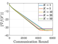
(a) $\rho=0.9664$

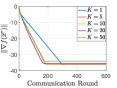
(b) $\rho=0.5946$

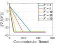
(c) $\rho=0$

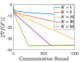
(d) Low

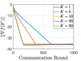
(e) Moderate

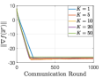
(f) High

Figure 1: Local DGT applied to the ridge logistic regression. First row: influence of network connectivity. Second row: influence of heterogeneity degree.

Influence of heterogeneity. $\bullet$ Data generalization. The local sample size is $n=100$ and the model dimension is set as $d=80$. All three groups adopt the same generation approach that $\bm{x}_{i}=\bm{x}_{b}+\bm{v}_{i},\forall i\in[m]$, where $\bm{x}_{b}\sim\mathcal{N}(\bm{0},\bm{I}_{d})$ and $\bm{v}_{i}\sim\mathcal{N}(0,\bm{I}_{d})$ are normal random vectors. For the $p$-th group ($p=1,2,3$), the samples are generated as follows to control the heterogeneity degree. For the first agent, its local features are i.i.d. generated as $\bm{a}_{1,j}\sim\mathcal{N}(\mathbf{0},\bm{I}_{d})$. Then for the $i$-th agent, we generate its feature as $\bm{a}_{i,j}=\bm{a}_{1,j}+\delta_{p}\cdot\mathcal{N}(\bm{0},\bm{I}_{d})$, $\forall i=2,\cdots,m$. The first group has low heterogeneity ($\delta_{1}=0.99$), the second group has moderate heterogeneity ($\delta_{2}=4$), and the last group exhibits high heterogeneity ($\delta_{3}=10^{4}$). We generate the label $y_{i,j}$ in the same way as the previous setting. $\bullet$ Network Setting. This setting maintains a fixed communication network with $\rho=0.5946$ for the above three different groups of datasets with varying degrees of heterogeneity. The results are given in the second row of Fig. 1, which shows less heterogeneity can improve the effectiveness of local updates.

(a) (M,0.85)

(b) (M,0)

(c) (L,0.85)

(d) (L,0)

(e) (M,0.85)

(f) (M,0)

(g) (L,0.85)

(h) (L,0)

Figure 2: Convergence for local DGT (top) and LED (bottom) for solving DRLR on “a9a” dataset. “L” and “M” denote low and moderate heterogeneity degree, respectively. The values 0 and 0.85 are values of $\rho$.

The experimental results illustrate local updates can effectively reduce communication complexity when the network connectivity is relatively good or data heterogeneity is mild. However, in cases where local updates are beneficial, increasing $K$ beyond certain thresholds offers marginal benefit in reducing communication costs. These observations corroborate the result in Theorem 1.

IV-B Local DGT for DRLR on real-world dataset

In this part, we use the same DRLR loss for binary classification on the real-world “a9a” dataset, which could be downloaded from LIBSVM repository [40]. We set the number of agents $m=50$ and set the same number of training samples for agents. $\bullet$ Data Distribution. The feature dimension is $d=122$ and the number of training samples is 15000, with 11500 and 3500 for class 1 and class 2, respectively. The number of test samples is 1281, with 935 and 346 for class 1 and class 2, respectively. We properly allocate samples among agents to construct two different degrees of heterogeneity. For higher heterogeneity, we allocate the training samples of the first 38 agents to be class 1, while the training samples of the remaining agents are class 2. For lower heterogeneity, we allocate data uniformly that there are 230 samples with class 1 and 70 samples with class 2 in each agent. $\bullet$ Network Setting. We conduct the local DGT on networks with two different connectivity $\rho=0.85$ and $\rho=0$ (fully connected). We set the regularization parameter $\mu=1$ in all cases and compare the performance of local DGT with the method LED [24], which is the latest decentralized method with local updates. The comparison between local DGT and LED for convergence and test accuracy is shown in Fig. 2 and Fig. 3, respectively.

(a) (M,0.85)

(b) (M,0)

(c) (L,0.85)

(d) (L,0)

(e) (M,0.85)

(f) (M,0)

(g) (L,0.85)

(h) (L,0)

Figure 3: Test accuracy for local DGT (top) and LED (bottom) for solving DRLR on “a9a” dataset. Here, “L” and “M” denote low and moderate heterogeneity degrees, respectively. The values 0 and 0.85 are values of $\rho$.

It can be observed that when network connectivity is sufficient, local DGT is more communication efficient than LED. As for test accuracy, because the total loss function of DRLR is strongly convex and has a unique solution, trajectories obtained from all cases converge the same test accuracy.

IV-C Over-parameterized linear regression

In this section, we conduct the over-parameterized least squares simulation to explore the usefulness of local updates for local DGT and local DGD. The local loss for the $i$-th agent is $f_{i}(\bm{x})=\frac{1}{2n}\|\bm{A}_{i}\bm{x}-\bm{b}_{i}\|^{2}$. We compare these methods in two settings with different degrees of data heterogeneity. The optimality measure is set as $\|\overline{\bm{x}}^{r}-\bm{x}^{\star}\|$, i.e., the distance to the minimum norm solution.

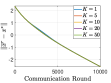
(a) $\rho=0.9676$

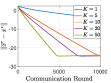
(b) $\rho=0.8924$

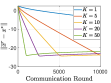
(c) $\rho=0$

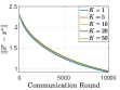
(d) $\rho=0.9676$

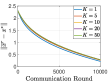
(e) $\rho=0.8924$

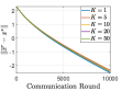
(f) $\rho=0$

Figure 4: Influence of network connectivity under moderate data heterogeneity. First row: local DGT. Second row: local DGD.

Moderate heterogeneity. The communication complexity is provided in Figure 4. As $\rho$ decreases, the first row shows increasing local updates in local DGT become more effective in reducing communication costs. In contrast, the second row reveals increasing local updates in local DGD is less useful. This can be explained by Theorem 3. When $\frac{\delta}{\mu}$ is large, Eq. (22) shows the communication complexity will be dominated by the second term that scales with $(\frac{\delta}{\mu})^{2}$. As such, increasing $K$ will not significantly reduce communication. However, the communication complexity of local DGT only scales with $\frac{\delta}{\mu}$, and consequently increasing $K$ is more effective compared to local DGD.

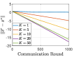
(a) $\rho=0.9664$

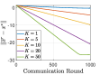
(b) $\rho=0.8924$

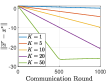
(c) $\rho=0$

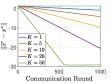
(d) $\rho=0.9664$

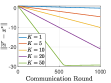
(e) $\rho=0.8924$

(f) $\rho=0$

Figure 5: Influence of network connectivity under low data heterogeneity. First row: local DGT. Second row: local DGD.

Figure 4 also shows the impact of network connectivity. In view of local DGT, Eq. (23) shows decreasing $\rho$ reduces the last two terms, thus increasing $K$ would be more efficient (first row). On the other hand, Eq. (22) shows increasing $\rho$ reduces the second term and improves the communication complexity for all choices of $K$ when it is dominating (second row).

Low heterogeneity. The communication complexity is shown in Figure 5. For local DGT, either increasing $K$ or decreasing $\rho$ helps reduce communication. For small $\rho$, the effectiveness of increasing $K$ is more significant. This can be explained by (23) for small $\delta$. For local DGD, increasing $K$ helps reduce communication, but reducing $\rho$ does not yield significant improvement. This is due to in (22) the first term is dominating for small $\delta$.

Comparing the two methods, we see Local DGT does not outperform DGD, and is even worse for poorly connected networks. This numerically validates our theoretical prediction (see comments around Eq. (22)): local DGD can be more communication efficient than DGT for problems with small $\delta$ and large $\rho$.

V Conclusions

We considered two decentralized optimization methods, DGT and DGD, and studied the effectiveness of employing multiple local updates in reducing communication costs. By studying local DGT for strongly convex problems and local DGD in the over-parameterization regime, our result reveals an interesting yet intuitive finding that the convergence rate of the algorithms will be affected by data heterogeneity through the second-order terms when the discrepancy of the first-order terms is eliminated. Through the expressions of the communication complexity, we demonstrated increasing local updates will be advantageous when the datasets are similar and network connectivity is relatively high.

References

- [1] X. Lian, C. Zhang, H. Zhang, C.-J. Hsieh, W. Zhang, and J. Liu, “Can decentralized algorithms outperform centralized algorithms? a case study for decentralized parallel stochastic gradient descent,” Advances in neural information processing systems, vol. 30, 2017.
- [2] S. Boyd, N. Parikh, E. Chu, B. Peleato, J. Eckstein et al., “Distributed optimization and statistical learning via the alternating direction method of multipliers,” Foundations and Trends® in Machine learning, vol. 3, no. 1, pp. 1–122, 2011.
- [3] A. H. Sayed et al., “Adaptation, learning, and optimization over networks,” Foundations and Trends® in Machine Learning, vol. 7, no. 4-5, pp. 311–801, 2014.
- [4] A. Nedic and A. Ozdaglar, “Distributed subgradient methods for multi-agent optimization,” IEEE Transactions on Automatic Control, vol. 54, no. 1, pp. 48–61, 2009.
- [5] A. Nedić, A. Olshevsky, and M. G. Rabbat, “Network topology and communication-computation tradeoffs in decentralized optimization,” Proceedings of the IEEE, vol. 106, no. 5, pp. 953–976, 2018.
- [6] B. McMahan, E. Moore, D. Ramage, S. Hampson, and B. A. y Arcas, “Communication-efficient learning of deep networks from decentralized data,” in Artificial intelligence and statistics. PMLR, 2017, pp. 1273–1282.
- [7] B. Woodworth, K. K. Patel, S. Stich, Z. Dai, B. Bullins, B. Mcmahan, O. Shamir, and N. Srebro, “Is local sgd better than minibatch sgd?” in International Conference on Machine Learning. PMLR, 2020, pp. 10 334–10 343.
- [8] B. E. Woodworth, K. K. Patel, and N. Srebro, “Minibatch vs local sgd for heterogeneous distributed learning,” Advances in Neural Information Processing Systems, vol. 33, pp. 6281–6292, 2020.
- [9] A. Koloskova, N. Loizou, S. Boreiri, M. Jaggi, and S. Stich, “A unified theory of decentralized sgd with changing topology and local updates,” in International Conference on Machine Learning. PMLR, 2020, pp. 5381–5393.
- [10] A. Nedic, A. Olshevsky, and W. Shi, “Achieving geometric convergence for distributed optimization over time-varying graphs,” SIAM Journal on Optimization, vol. 27, no. 4, pp. 2597–2633, 2017.
- [11] J. Xu, S. Zhu, Y. C. Soh, and L. Xie, “Augmented distributed gradient methods for multi-agent optimization under uncoordinated constant stepsizes,” in 2015 54th IEEE Conference on Decision and Control (CDC). IEEE, 2015, pp. 2055–2060.
- [12] P. Di Lorenzo and G. Scutari, “Next: In-network nonconvex optimization,” IEEE Transactions on Signal and Information Processing over Networks, vol. 2, no. 2, pp. 120–136, 2016.
- [13] C. Zhang, S. Bengio, M. Hardt, B. Recht, and O. Vinyals, “Understanding deep learning (still) requires rethinking generalization,” Communications of the ACM, vol. 64, no. 3, pp. 107–115, 2021.
- [14] S. Ma, R. Bassily, and M. Belkin, “The power of interpolation: Understanding the effectiveness of sgd in modern over-parametrized learning,” in International Conference on Machine Learning. PMLR, 2018, pp. 3325–3334.
- [15] T. Qin, S. R. Etesami, and C. A. Uribe, “Decentralized federated learning for over-parameterized models,” in 2022 IEEE 61st Conference on Decision and Control (CDC). IEEE, 2022, pp. 5200–5205.
- [16] K. Mishchenko, G. Malinovsky, S. Stich, and P. Richtárik, “Proxskip: Yes! local gradient steps provably lead to communication acceleration! finally!” in International Conference on Machine Learning. PMLR, 2022, pp. 15 750–15 769.
- [17] Y. Huang and J. Xu, “On the computation-communication trade-off with a flexible gradient tracking approach,” arXiv preprint arXiv:2306.07159, 2023.
- [18] S. P. Karimireddy, S. Kale, M. Mohri, S. Reddi, S. Stich, and A. T. Suresh, “Scaffold: Stochastic controlled averaging for federated learning,” in International Conference on Machine Learning. PMLR, 2020, pp. 5132–5143.
- [19] F. Haddadpour, M. M. Kamani, A. Mokhtari, and M. Mahdavi, “Federated learning with compression: Unified analysis and sharp guarantees,” in International Conference on Artificial Intelligence and Statistics. PMLR, 2021, pp. 2350–2358.
- [20] K. Yuan, Q. Ling, and W. Yin, “On the convergence of decentralized gradient descent,” SIAM Journal on Optimization, vol. 26, no. 3, pp. 1835–1854, 2016.
- [21] E. D. H. Nguyen, S. A. Alghunaim, K. Yuan, and C. A. Uribe, “On the performance of gradient tracking with local updates,” arXiv preprint arXiv:2210.04757, 2022.
- [22] Y. Liu, T. Lin, A. Koloskova, and S. U. Stich, “Decentralized gradient tracking with local steps,” arXiv preprint arXiv:2301.01313, 2023.
- [23] S. Ge and T.-H. Chang, “Gradient and variable tracking with multiple local sgd for decentralized non-convex learning,” arXiv preprint arXiv:2302.01537, 2023.
- [24] S. A. Alghunaim, “Local exact-diffusion for decentralized optimization and learning,” arXiv preprint arXiv:2302.00620, 2023.
- [25] B. Song, I. Tsaknakis, C.-Y. Yau, H.-T. Wai, and M. Hong, “Distributed optimization for overparameterized problems: Achieving optimal dimension independent communication complexity,” Advances in Neural Information Processing Systems, vol. 35, pp. 6147–6160, 2022.
- [26] P. Khanduri, H. Yang, M. Hong, J. Liu, H. T. Wai, and S. Liu, “Decentralized learning for overparameterized problems: A multi-agent kernel approximation approach,” in International Conference on Learning Representations, 2021.
- [27] Y. Deng, M. M. Kamani, and M. Mahdavi, “Local sgd optimizes overparameterized neural networks in polynomial time,” in International Conference on Artificial Intelligence and Statistics. PMLR, 2022, pp. 6840–6861.
- [28] B. Song, P. Khanduri, X. Zhang, J. Yi, and M. Hong, “Fedavg converges to zero training loss linearly: The power of overparameterized multi-layer neural networks,” 2023.
- [29] S. S. Kia, B. Van Scoy, J. Cortes, R. A. Freeman, K. M. Lynch, and S. Martinez, “Tutorial on dynamic average consensus: The problem, its applications, and the algorithms,” IEEE Control Systems Magazine, vol. 39, no. 3, pp. 40–72, 2019.
- [30] J. Zeng and W. Yin, “On nonconvex decentralized gradient descent,” IEEE Transactions on signal processing, vol. 66, no. 11, pp. 2834–2848, 2018.
- [31] Y. Sun, G. Scutari, and A. Daneshmand, “Distributed optimization based on gradient tracking revisited: Enhancing convergence rate via surrogation,” SIAM Journal on Optimization, vol. 32, no. 2, pp. 354–385, 2022.
- [32] B. Li, S. Cen, Y. Chen, and Y. Chi, “Communication-efficient distributed optimization in networks with gradient tracking and variance reduction,” The Journal of Machine Learning Research, vol. 21, no. 1, pp. 7331–7381, 2020.
- [33] B. E. Woodworth, J. Wang, A. Smith, B. McMahan, and N. Srebro, “Graph oracle models, lower bounds, and gaps for parallel stochastic optimization,” Advances in neural information processing systems, vol. 31, 2018.
- [34] Q. Nguyen and M. Hein, “Optimization landscape and expressivity of deep cnns,” in International conference on machine learning. PMLR, 2018, pp. 3730–3739.
- [35] Q. Nguyen, M. Mondelli, and G. F. Montufar, “Tight bounds on the smallest eigenvalue of the neural tangent kernel for deep relu networks,” in International Conference on Machine Learning. PMLR, 2021, pp. 8119–8129.
- [36] Z. Charles and D. Papailiopoulos, “Stability and generalization of learning algorithms that converge to global optima,” in International conference on machine learning. PMLR, 2018, pp. 745–754.
- [37] C. Liu, L. Zhu, and M. Belkin, “Loss landscapes and optimization in over-parameterized non-linear systems and neural networks,” Applied and Computational Harmonic Analysis, vol. 59, pp. 85–116, 2022.
- [38] O. Shamir, “The implicit bias of benign overfitting,” Journal of Machine Learning Research, vol. 24, no. 113, pp. 1–40, 2023.
- [39] S. Gunasekar, J. Lee, D. Soudry, and N. Srebro, “Characterizing implicit bias in terms of optimization geometry,” in International Conference on Machine Learning. PMLR, 2018, pp. 1832–1841.
- [40] C.-C. Chang and C.-J. Lin, “Libsvm: a library for support vector machines,” ACM transactions on intelligent systems and technology (TIST), vol. 2, no. 3, pp. 1–27, 2011.