Data-Driven Approximation of Stationary Nonlinear Filters
with Optimal Transport Maps

Abstract

The nonlinear filtering problem is concerned with finding the conditional probability distribution (posterior) of the state of a stochastic dynamical system, given a history of partial and noisy observations. This paper presents a data-driven nonlinear filtering algorithm for the case when the state and observation processes are stationary. The posterior is approximated as the push-forward of an optimal transport (OT) map from a given distribution, that is easy to sample from, to the posterior conditioned on a truncated observation window. The OT map is obtained as the solution to a stochastic optimization problem that is solved offline using recorded trajectory data from the state and observations. An error analysis of the algorithm is presented under the stationarity and filter stability assumptions, which decomposes the error into two parts related to the truncation window during training and the error due to the optimization procedure. The performance of the proposed method, referred to as optimal transport data-driven filter (OT-DDF), is evaluated for several numerical examples, highlighting its significant computational efficiency during the online stage while maintaining the flexibility and accuracy of OT methods in nonlinear filtering.

I Introduction

A nonlinear filtering problem consists of two processes: (i) a hidden Markov process $\{X_{1},X_{2},\ldots\}$ that represents the state of a dynamical system; and (ii) an observed random process $\{Y_{1},Y_{2},\ldots\}$ that represents the noisy sensory measurements of the state. The job of a nonlinear filter is to numerically approximate the posterior distribution, i.e. the conditional probability distribution of the state $X_{t}$ given a history of noisy measurements $\{Y_{t},Y_{t-1},\ldots,Y_{1}\}$, for $t=1,2,\ldots$. The exact posterior admits a recursive update law that facilitates the design of nonlinear filtering algorithms [8]. Denoting the posterior at time $t$ by $\pi_{t}$, the recursive update law may be expressed as

$$\pi_{t}=F_{t}(Y_{t})(\pi_{t-1})$$ (1)

where $F_{t}(Y_{t})$ is a $Y_{t}$-dependent map on the space of probability distributions that consists of two operations: the propagation step that updates the posterior according to the dynamic model and the conditioning step that updates the posterior according to Bayes’ rule; see Sec. II-A for details and a brief review. The initial distribution $\pi_{0}$ is the probability distribution of the initial condition $X_{0}$.

Nonlinear filtering algorithms carry out different numerical approximations of the update step (1). Kalman filter (KF) [22], and its extensions [4, 16, 7], rely on a Gaussian approximation of the joint distribution of the state and observation, thereby, simplifying (1) to an update for a mean vector and a covariance matrix. Due to the Gaussian approximation, the performance of KF type algorithms is limited to linear dynamical systems with additive Gaussian noise. Sequential importance re-sampling particle filters  [18, 15] approximate the posterior with a weighted empirical distribution of a large number of particles. While they provide an asymptotically exact solution in the limit of infinitely many particles, they suffer from the weight-degeneracy issues in high dimensions [6, 5, 27]. Coupling and controlled interacting particle system approaches [11, 37, 28, 12, 36, 26, 30, 29, 32] avoid weight degeneracy by replacing the importance sampling step with a control law/coupling that updates the location of the particles with uniform weights. However, the main bottleneck of these types of algorithms becomes the online computation of the control law/coupling.

This paper is built upon our recent work that proposes an optimal transport (OT) variational formulation of the Bayes’ law to construct nonlinear filtering algorithms [31, 1, 19, 2]. In this formulation, the update step (1) is replaced with a push-forward of a map $T_{t}$ following

$$\pi_{t}=T_{t}(\cdot,Y_{t})_{\#}\pi_{t-1},$$ (2)

and the map $T_{t}$ is obtained by solving a stochastic optimization problem that aims at finding the OT map from $\pi_{t-1}$ to $\pi_{t}$ (see Sec. III-A for details). This approach, which is referred to as the OT particle filter (OTPF), has two main appealing features: (i) it only requires samples from the joint distribution of the state $X_{t}$ and the observations $Y_{t}$, without the need for the analytical model of the observation likelihood and dynamics, i.e. given a sample $X_{t-1}$, we need an oracle or a simulator that samples $X_{t}$ and $Y_{t}$; (ii) it allows for the utilization of neural networks to enhance the representation power of the transport maps $T_{t}$ to model complex and multi-modal probability distributions. Due to these features, the OTPF is numerically favorable for problem settings that involve multi-modal and high-dimensional posterior distributions [2]. However, the better performance comes with the cost of solving a stochastic optimization problem online at each time $t$.

In this paper, we propose an algorithm, referred to as OT data-driven filter (OT-DDF), that improves upon OTPF in two critical aspects:

1. We make the algorithm completely data-driven, by only requiring recorded data from the state and observations without active usage of a simulator/oracle.

2. We make the online computations very light by replacing the online optimization with an offline training stage that finds a fixed map $T$ that conditions on a truncated measurement history $\{Y_{t},Y_{t-1},\ldots,Y_{t-w+1}\}$ for some window size $w$.

These improvements become possible by making two critical assumptions about the model: (A1) the process $(X_{t},Y_{t})$ is stationary; (A2) the filter dynamics (1) is stable. Precise statements of the assumptions appear in Sec. II-B.

The rest of the paper is organized as follows: Sec. II includes the mathematical setup and the modeling assumptions; Sec. III contains the proposed methodology accompanied with an error analysis; and section IV presents several numerical experiments that serve as proof of concept and compares the proposed algorithm with alternative approaches.

II Problem Formulation

II-A Mathematical setup

In this paper, we consider a discrete-time stochastic dynamic system given by the update equations

$$X_{t} \sim a_{t}(\cdot|X_{t-1}),\quad X_{0}\sim\pi_{0}$$ (3a)

$$Y_{t} \sim h_{t}(\cdot|X_{t})$$ (3b)

for $t=1,2,\ldots$ where $X_{t}\in\mathbb{R}^{n}$ is the hidden state of the system, $Y_{t}\in\mathbb{R}^{m}$ is the observation, $\pi_{0}$ is the probability distribution for the initial state $X_{0}$, $a_{t}(x^{\prime}|x)$ is the transition kernel from $X_{t-1}=x$ to $X_{t}=x^{\prime}$, and $h_{t}(y|x)$ is the likelihood of observing $Y_{t}=y$ given $X_{t}=x$.

The dynamic and observation models are used to introduce the following propagation and conditioning operators

$$\text{(propagation)}~{}\pi\mapsto\mathcal{A}_{t}(\pi) :=\int_{\mathbb{R}^{n}}a_{t}(\cdot|x)\pi(x)dx,$$ (4a)

$$\text{(conditioning)}~{}\pi\mapsto\mathcal{B}_{t}(y)(\pi) :=\frac{h_{t}(y|\cdot)\pi(\cdot)}{\int_{\mathbb{R}^{n}}h_{t}(y|x)\pi(x)dx},$$ (4b)

for an arbitrary probability distribution $\pi$. The propagation operator $\mathcal{A}_{t}$ represents the update for the distribution of the state according to the dynamic model (3a), and the conditioning operator $\mathcal{B}_{t}$ represents Bayes’ rule that carries out the conditioning according to the observation model (3b). The composition of these maps is denoted by

$$F_{t}(y):=\mathcal{B}_{t}(y)\circ\mathcal{A}_{t}$$

and consecutive application of $F_{t}$ is denoted by

$$F_{t,s}(y_{t},\ldots,y_{s+1})\!:=F_{t}(y_{t})\circ F_{t-1}(y_{t-1})\circ\ldots\circ F_{s+1}(y_{s+1}),$$

for $t>s$. For simplicity, hereon, we introduce the compact notation $y_{t,s}:=\{y_{t},\ldots,y_{s+1}\}$ for $t>s\geq 0$.

We are interested in two conditional distributions:

• Exact posterior: The exact posterior $\pi_{t}$ is defined as the conditional distribution of $X_{t}$ given $Y_{t,0}:=\{Y_{t},\ldots,Y_{1}\}$, i.e.

  $$\pi_{t}(\cdot):=\mathbb{P}(X_{t}\in\cdot\mid Y_{t,0}).$$ (5)

  In terms of our notation earlier, it can be identified via

  $$\pi_{t}=F_{t,0}(Y_{t,0})(\pi_{0}).$$ (6)

• Truncated posterior: The truncated posterior, denoted by $\pi_{t,s}^{\mu}$, is defined as the conditional distribution of $X_{t}$, given $Y_{t,s}:=\{Y_{s+1},\ldots,Y_{t}\}$, with the prior distribution $X_{s}\sim\mu$, i.e.

  $$\pi_{t,s}^{\mu}(\cdot):=\mathbb{P}_{X_{s}\sim\mu}(X_{t}\in\cdot\mid Y_{t,s}).$$ (7)

  It is given by the equation

  $$\pi_{t,s}^{\mu}=F_{t,s}(Y_{t,s})(\mu).$$ (8)

II-B Modelling assumptions

To ensure the applicability of our proposed method, we make the following two critical assumptions.

Assumption 1

The stochastic process $(X_{t},Y_{t})$ is stationary. In particular, the model (3) is time invariant, i.e. $a_{t}=a$ and $h_{t}=h$ for all $t=1,2,\ldots$, and $\pi_{0}$ is equal to the unique stationary distribution of $\mathcal{A}$, i.e. $\mathcal{A}\pi_{0}=\pi_{0}$. The stationary distribution has finite second moments, and it admits a density with respect to the Lebesgue measure.

This assumption implies that

$$F_{t,s}=F_{t-s,0},~{}\forall t>s\geq 0.$$ (9)

Remark 1

The assumption that $\pi_{0}$ is equal to the stationary distribution is made to facilitate the error analysis in Sec. III-C. This assumption may be replaced with geometric ergodicity of the Markov process $X_{t}$ at the cost of the extra term appearing in the error bound (21). In our numerical simulations, we simulate the true model for a burn-in period to ensure the probability distribution of $X_{t}$ is close to being stationary.

The second assumption is related to the stability of the filtering dynamics (6). Consider the following metric on (possibly random) probability measures $\mu,\nu$:

$$d(\mu,\nu):=\sup_{g\in\mathcal{G}}\sqrt{\mathbb{E}\left|\int gd\mu-\int gd\nu\right|^{2}}$$ (10)

where the expectation is over the possible randomness of the probability measures $\mu$ and $\nu$, and $\mathcal{G}:=\{g:\mathbb{R}^{n}\to\mathbb{R};\,|g(x)|\leq 1,|g(x)-g(x^{\prime})|\leq\|x-x^{\prime}\|,\quad\forall x,x^{\prime}\}$ is the space of functions that are uniformly bounded by one and uniformly Lipschitz with a constant smaller than one (this metric is also known as the dual bounded-Lipschitz distance [34]).

Assumption 2

The filter is uniformly geometrically stable, i.e. $\exists\lambda\in(0,1)$ and a positive constant $C>0$ such that for all $\mu,\nu$ and $t>s\geq 0$ it holds that

$$d(F_{t,s}(Y_{t,s})(\mu),F_{t,s}(Y_{t,s})(\nu))\leq C\lambda^{t-s}d(\mu,\nu).$$ (11)

Remark 2

The filter stability is a natural assumption that ensures the applicability of a numerical filtering algorithm. Similar stability assumptions also appear in [13, 34] for the error analysis of particle filters. However, finding necessary and sufficient conditions that ensure filter stability is challenging; see [1, Remark 1] and [33, 10, 23] for example conditions that ensure filter stability.

II-C Objective

In the usual filtering setup, the dynamic and observation models, $a$ and $h$, are known. However, we assume that these models are unknown. Instead, we have access to $J$ recorded independent state-observation trajectories of length $t_{f}$, i.e. $\{X^{j}_{0},(X^{j}_{1},Y^{j}_{1}),\ldots,(X^{j}_{t_{f}},Y^{j}_{t_{f}})\}_{j=1}^{J}$. Then, our objective is

Given: $$\left\{X^{j}_{0},(X^{j}_{1},Y^{j}_{1}),\ldots,(X^{j}_{t_{f}},Y^{j}_{t_{f}})\right\}_{j=1}^{J}$$

Approximate: $$\pi_{t}=\mathbb{P}(X_{t}\in\cdot\mid Y_{t},\ldots,Y_{1})\quad\forall t\geq 0,$$

$$\text{for a new set of observations }\{Y_{t},\dots,Y_{1}\}.$$

III The Optimal transport Data-Driven Filter

III-A OT formulation for conditioning

The proposed methodology is based on the OT formulation of the Bayes’ law that is used to represent conditional distributions as a push-forward of OT maps [31, 21]. Consider a joint probability distribution $\nu_{XY}$ and its conditional $\nu_{X|Y}$. Then, the goal is to find a map $\overline{T}$ such that

$$\nu_{X|Y}(\cdot|y)=\overline{T}(\cdot,y)_{\#}\eta_{X}$$ (12)

where $\eta_{X}$ is an arbitrary probability distribution. Furthermore, the map $\overline{T}(\cdot,y)$ is the OT map from $\eta_{X}$ to $\nu_{X|Y}(\cdot|y)$ for $\nu_{Y}$-almost every $y$; where we used $\nu_{Y}$ to denote the $Y$-marginal of $\nu_{XY}$. The OT formulation is useful because the map $\overline{T}$ can be obtained as the solution to a max-min stochastic optimization problem

$$\max_{f\in c\text{-Concave}_{x}}\,\min_{T\in\mathcal{M}(\eta)}\,J_{\eta,\nu}(f,T)$$ (13)

where $\eta=\eta_{X}\otimes\nu_{Y}$ is the independent coupling of $\eta_{X}$ and $\nu_{Y}$, $\mathcal{M}(\eta)$ denotes the set of $\eta$-measurable maps, $f\in c\text{-Concave}_{x}$ means $x\mapsto\frac{1}{2}\|x\|^{2}-f(x,y)$ is convex in $x$ for all $y$ [35, Def. 2.33], and the objective function

$$J_{\eta,\nu}(f,T) :=\mathbb{E}_{(X,Y)\sim\nu}[f(X,Y)]+$$

$$\mathbb{E}_{(X,Y)\sim\eta}[\frac{1}{2}\|T(X,Y)-X\|^{2}-f(T(X,Y),Y)].$$

The well-posedness of the max-min problem is stated in the following theorem.

Theorem 1

If $\eta_{X}$ has a finite second moment and it is absolutely continuous with respect to the Lebesgue measure, then the max-min problem (13) admits a unique optimal pair $(\overline{f},\overline{T})$, modulo additive constant shifts for $\overline{f}$, and the relationship (12) holds $\nu_{Y}$-almost everywhere.

Remark 3

The proof of this result appears in [2, Proposition 2.3] which is an extension of the existing results [9, Theorem 2.3] and [24, Theorem 2.4]. The extension to the Riemannian manifold and infinite-dimensional functional space settings appear in [19] and [21], respectively.

The following result relates the error in approximating the conditional distribution with the optimality gap of solving the max-min problem. In particular, let $(\hat{f},\hat{T})$ be the output of an algorithm that approximately solves (13) and consider $\hat{T}(\cdot,Y)_{\#}\eta_{X}$ as an approximation to $\nu_{X|Y}(\cdot|y)$. Define the max-min optimality gap

$$\epsilon(\hat{f},\hat{T}):= J_{\eta,\nu}(\hat{f},\hat{T})-\min_{T}J_{\eta,\nu}(\hat{f},T)$$ (14)

$$+ \max_{f}\min_{T}J_{\eta,\nu}(f,T)-\min_{T}J_{\eta,\nu}(\hat{f},T),$$

where the first term specifies the gap in the minimization, and the second term specifies the gap in the maximization. Then we have the following lemma, the proof of which is given in  [2, Proposition 2.4].

Lemma 1

Consider the assumptions of Theorem 1. Then, for any pair $(\hat{f},\hat{T})$ such that $x\mapsto\frac{1}{2}\|x\|^{2}-\hat{f}(x,y)$ is $\alpha$-strongly convex in $x$ for all $y$, we have the bound

$$d(\hat{T}(\cdot,Y)_{\#}\eta_{X},\nu_{X|Y}(\cdot|Y))\leq\sqrt{\frac{4}{\alpha}\epsilon(\hat{f},\hat{T})}.$$ (15)

III-B Proposed methodology

The proposed methodology is summarized in four steps:

Step 1: We propose to approximate the truncated posterior (7) instead of the exact posterior (5). This step introduces an error that is bounded due to filter stability Assumption 2. In particular, replacing $\nu$ by $\pi_{s}$ in (11), and the fact that $F_{t,s}(Y_{t,s})(\pi_{s})=\pi_{t}$ and $F_{t,s}(Y_{t,s})(\mu)=\pi^{\mu}_{t,s}$ , we conclude the bound

$$d(\pi^{\mu}_{t,s},\pi_{t})\leq C\lambda^{t-s}d(\mu,\pi_{s}).$$ (16)

The error bound can be made arbitrarily small by choosing a large window size $w:=t-s$ and assuming a uniform bound on $d(\mu,\pi_{s})$ for all $s$.

Step 2: We use the OT formulation (12) with the min-max problem (13) to characterize the truncated posterior. In order to do so, we choose the target distribution $\nu$ to be the joint distribution of $(X_{t},Y_{t,s})$ where $X_{t}$ and $Y_{t,s}:=\{Y_{t},\ldots,Y_{s+1}\}$ are generated using the stochastic model (3a)-(3b) with $X_{s}\sim\mu$. And we choose the source distribution $\eta$ to be equal to the independent coupling of $X_{s}\sim\mu$ (i.e. $\eta_{X}=\mu$) and $Y_{t,s}$, i.e.

$$\nu =\text{Law}(X_{t},Y_{t,s}) \text{with}\quad X_{s}\sim\mu,$$ (17)

$$\eta =\text{Law}(X_{s})\otimes\text{Law}(Y_{t,s})\quad \text{with}\quad X_{s}\sim\mu.$$

With this setup, the conditional distribution $\nu_{X|Y}$ equals the truncated posterior $\pi_{t,s}^{\mu}$. Let $\overline{T}^{\mu}_{t,s}$ denote the optimizer of the max-min problem (13) with $\nu$ and $\eta$ chosen as explained above. Then, the relationship (12) implies that

$$\pi_{t,s}^{\mu}(\cdot)=\overline{T}_{t,s}^{\mu}(\cdot,Y_{t,s})_{\#}\mu.$$

Using the fact that $\pi_{t,s}^{\mu}$ is also given by (8), we can also conclude the identity

$$F_{t,s}(Y_{t,s})(\mu)=\overline{T}_{t,s}^{\mu}(\cdot,Y_{t,s})_{\#}\mu,$$ (18)

for all probability distributions $\mu$.

Step 3: By the time-invariance Assumption 1 and the identity (18) we conclude, with $w=t-s$, that

$$\overline{T}^{\mu}_{t,s}=\overline{T}^{\mu}_{w,0}\quad\forall\,t>s\geq 0.$$

Step 4: We use the recorded data to numerically approximate the map $\overline{T}^{\mu}_{w,0}$ by solving the max-min problem (13). In this problem, the target distribution $\nu$ is equal to the joint distribution of $(X_{w},Y_{w,0})$ with $X_{0}\sim\mu$ and the source distribution $\eta$ is equal to the independent coupling of $X_{0}$ and $Y_{w,0}$. The source and target distributions are empirically approximated as

$$\nu \approx\hat{\nu}:=\frac{1}{J}\sum_{j=1}^{J}\delta_{(X^{j}_{w},Y^{j}_{w,0})},~{}\eta\approx\hat{\eta}:=\frac{1}{J}\sum_{j=1}^{J}\delta_{(X^{\sigma_{j}}_{0},Y^{j}_{w,0})}$$ (19)

where $\{X^{j}_{0},(X^{j}_{1},Y^{j}_{1}),\ldots,(X^{j}_{w},Y^{j}_{w})\}_{j=1}^{J}$ are independent realizations of the state and observation available from recorded data, and $\{\sigma_{1},\ldots,\sigma_{J}\}$ is a random permutation of $\{1,2,\ldots,N\}$. We use stochastic optimization methods to approximately solve the resulting optimization problem by searching for the functions $f$ and map $T$ inside the parameterized classes $\mathcal{F}$ and $\mathcal{T}$ respectively (algorithm details appear in Sec. IV-A). We denote the resulting approximate pair by $(\hat{f}^{\mu}_{w,0},\hat{T}^{\mu}_{w,0})$, i.e.

$$(\hat{f}^{\mu}_{w,0},\hat{T}^{\mu}_{w,0})\leftarrow\max_{f\in\mathcal{F}}\,\min_{T\in\mathcal{T}}\,J_{\hat{\eta},\hat{\nu}}(f,T).$$ (20)

Summary: The four-step procedure is summarized as

$$\pi_{t}\overset{(1)}{\approx}\pi_{t,s}^{\mu} \overset{(2)}{=}\overline{T}^{\mu}_{t,s}(\cdot,Y_{t,s})_{\#}\mu$$

$$\overset{(3)}{=}\overline{T}^{\mu}_{w,0}(\cdot,Y_{t,s})_{\#}\mu\overset{(4)}{\approx}\hat{T}^{\mu}_{w,0}(\cdot,Y_{t,s})_{\#}\mu,$$

where the first step is approximation due to truncation, the second step is identity using the OT formulation, the third step is identity using the stationarity of the model, and the fourth step is numerical and algorithmic approximation.

III-C Error analysis

The objective of the error analysis is to bound the error between the exact posterior $\pi_{t}$ and the approximation $\hat{T}^{\mu}_{w}(\cdot,Y_{t,s})_{\#}\mu$ obtained from the four step procedure. Two steps of the procedure involve approximation. The first step is due to the truncation, and the fourth step is due to approximation in solving the max-min problem. The error, due to the first step, is bounded using the filter stability according to (16). The error, due to the second step, is bounded by the optimality gap using Lemma 1. The two results are combined to conclude an error bound under the following assumptions about the algorithm.

Assumption 3

The following conditions, regarding the algorithm, hold:

1. $\mu$ is equal to the stationary distribution of $X_{t}$.

2. $\exists M>0$ such that $d(\pi_{t},\mu)<M$ for all $t$.

3. $x\mapsto\frac{1}{2}\|x\|^{2}-\hat{f}_{w,0}^{\mu}(x,y)$ is $\alpha$-strongly convex in $x$ for all $y$.

Proposition 1

Consider a window side $w>0$ and suppose Assumptions 1, 2, and 3 hold. Then, for all $t>w$,

$$d(\hat{T}^{\mu}_{w,0}(\cdot,Y_{t,t-w})_{\#}\mu,\pi_{t})\leq C\lambda^{w}M+\sqrt{\frac{4}{\alpha}{\mathbb{E}}\epsilon(\hat{f}^{\mu}_{w,0},\hat{T}_{w,0}^{\mu})},$$ (21)

where the expectation is with respect to the randomness of training data and possibly the optimization procedure.

Remark 4

The first term in the bound is due to the truncation and becomes small as the window size $w$ increases. The second term depends on the optimality gap, and it is expected to decrease as the class of functions $\mathcal{F,T}$ becomes more expressive and the number of samples $J$ becomes large. Analysis of the optimality gap is the subject of ongoing work, and it is expected to follow from existing results for statistical generalization of optimal transport map estimation in [14] and approximation theory in [3].

Proof:

For simplicity, introduce the notation $\hat{S}:=\hat{T}^{\mu}_{w,0}(\cdot,Y_{t,t-w})$ and $\overline{S}:=\overline{T}^{\mu}_{w,0}(\cdot,Y_{t,t-w})$. Upon the application of the triangle inequality and the identity $\pi_{t,t-w}^{\mu}=\overline{S}_{\#}\mu$, we obtain the decomposition

$$d( \hat{S}_{\#}\mu,\pi_{t})\leq d(\hat{S}_{\#}\mu,\overline{S}_{\#}\mu)+d(\pi^{\mu}_{t,t-w},\pi_{t}).$$

Application of the bound (16) and Assumption A3b on $d(\pi^{\mu}_{t,t-w},\pi_{t})$ concludes the first term in (21). Application of inequality (15) to $d(\hat{S}_{\#}\mu,\overline{S}_{\#}\mu)$ concludes the second term in (21). Assumption A3a about the probability distribution $\mu$ is required to ensure that the probability distribution of the observation process $\nu_{Y}$ that is used for the max-min optimization is equal to the probability distribution of $Y_{t,t-w}$ that comes from the true model (3).  

IV Numerics

IV-A The numerical algorithm

The OT-DDF algorithm consists of two stages: (i) an offline stage which approximately solves (20) to obtain the transport map $\hat{T}^{\mu}_{w,0}$; (ii) an online stage which uses the truncated history of observations $Y_{t,t-w}$ and the learned map $\hat{T}^{\mu}_{w,0}$ to approximate the posterior $\pi_{t}$ for each time $t$.

In the offline stage, we use the ADAM stochastic optimization algorithm to solve (20). The algorithm consists of inner and outer loops. The inner loop consists of $k_{inner}$ iterations of ADAM to update the map $T$, while the outer loop consists of $k_{outer}$ iterations of ADAM to update $f$. The functions $f$ and $T$ are parameterized with neural networks with architectures described separately for each example. The samples $(X^{j}_{t_{0}},Y^{j}_{t_{0}+w,t_{0}})_{j=1}^{J}$ are used to form the approximation of $\hat{\nu}$ and $\hat{\eta}$ in (19). A burn-in time $t_{0}$ is included to ensure that the training data is stationary and assumption A3.a is satisfied approximately. The offline stage is summarized in Algorithm 1.

The subsequent stage is the online stage, where the output map $\hat{T}^{\mu}_{w,0}$ of algorithm 1 is used to approximate the posterior $\pi_{t}$ using the observations $Y_{t}$ that are received online.

In particular, the posterior $\pi_{t}$ is approximated with the empirical measure $\frac{1}{N}\sum_{i=1}^{N}\delta_{X^{i}_{t}}$ where

$${{X}}_{t}^{i}=\hat{T}^{\mu}_{w,0}(X_{t_{0}}^{i},Y_{t,t-w}),$$

and $\{X^{i}_{t_{0}}\}_{i=1}^{N}$ are $N$ random samples from $\{X^{j}_{t_{0}}\}_{j=1}^{J}$.

Algorithm 1 Offline Training of OT-DDF

  Input: Recorded data $\{X^{j}_{0},(X^{j}_{1},Y^{j}_{1}),\ldots,(X^{j}_{w},Y^{j}_{w})\}_{j=1}^{J}$, burn-in time $t_{0}$, window $w$, batch size $b_{s}$, architecture, optimizer and learning rates for $f,T$,inner and outer loop iterations $k_{inner}$, $k_{outer}$.

  Initialize: initialize neural net $f,T$ weights $\theta_{f},\theta_{T}$.

  Create a random permutation $\{\sigma_{i}\}_{i=1}^{J}$

  for $k=1$ to $k_{outer}$ do

     Select random batch $(X_{t_{0}}^{\sigma_{i}},X_{t_{0}+w}^{i},Y_{t_{0}+w,t_{0}}^{i})_{i=1}^{b_{s}}$

     Define $T^{i}=T(X_{t_{0}}^{\sigma_{i}},Y_{t_{0}+w,t_{0}}^{i})$ for $i=1,\ldots,b_{s}$

     for $j=1$ to $k_{inner}$ do

        Update $\theta_{T}$ to minimize $\frac{1}{b_{s}}\sum_{i=1}^{b_{s}}\big{[}\frac{1}{2}\|X_{t_{0}}^{\sigma_{i}}-T^{i}\|^{2}-f(T^{i},Y_{t_{0}+w,t_{0}}^{i})\big{]}$

     end for

     Update $\theta_{f}$ to minimize$\frac{1}{b_{s}}\sum_{i=1}^{b_{s}}\big{[}-f(X_{t_{0}+w}^{i},Y_{t_{0}+w,t_{0}}^{i})+f(T^{i},Y_{t_{0}+w,t_{0}}^{i})\big{]}$

  end for

  Output: Map $\hat{T}^{\mu}_{w,0}=T$.

The proposed OT-DDF method is evaluated against three other algorithms: the Ensemble Kalman filter (EnKF) [17], OTPF [1, 2], and the sequential importance resampling (SIR) PF [15]. The details for all of the three algorithms appear in [2], and the numerical code used to produce the results is available online.

IV-B Linear dynamics with linear and quadratic observation models

Consider

$$X_{t} =\begin{bmatrix}\alpha&\sqrt{1-\alpha^{2}}\\ -\sqrt{1-\alpha^{2}}&\alpha\end{bmatrix}X_{t-1}+\sigma V_{t}$$ (22a)

$$Y_{t} =h(X_{t})+\sigma W_{t}$$ (22b)

for $t=1,2,\dots$ where $X_{t}\in\mathbb{R}^{2}$, $Y_{t}\in\mathbb{R}$, $\{V_{t}\}_{t=1}^{\infty}$ and $\{W_{t}\}_{t=1}^{\infty}$ are i.i.d sequences of $2$-dimensional and one-dimensional standard Gaussian random variables, $\alpha=0.9$ and $\sigma^{2}=0.1$. Two observation functions are of interest:

$$h(X_{t})=X_{t}(1),\quad\text{and}\quad h(X_{t})=X_{t}(1)^{2}$$

where $X_{t}(1)$ is the first component of the vector $X_{t}$. We refer to these observation models as linear and quadratic, respectively.

We implemented algorithm 1 with different window sizes $w=1,10,50$. The burn-in time was $t_{0}=100-w$. The functions $f$ and $T$ were parameterized as ResNets with one and two blocks of size $64$ and $48$, respectively. The optimization learning rates for $f$ and $T$ was $10^{-3}$ and $5\times 10^{-4}$ with $k_{inner}=10$, $k_{outer}=12000$, and batch size $b_{s}=64$.

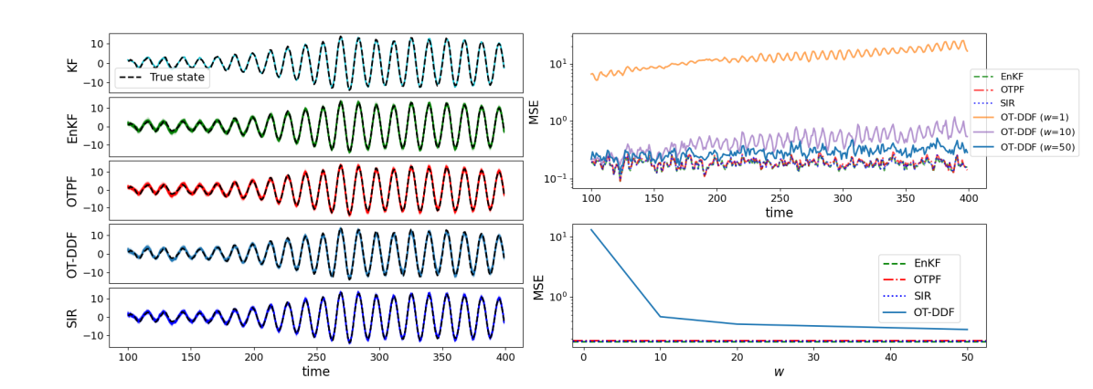
Figure 1: Numerical results for the linear dynamic example with linear observation function. The left column shows the trajectory of the second component of the particles along with the trajectory of the true state, where $w=50$ for the OT-DDF method. The right column shows the MSE in estimating the state as a function of time in the upper corner and as a function of the window size $w$ in the lower corner.

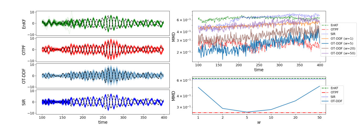
Figure 2: Numerical results for the linear dynamic example with quadratic observation function. The left column shows the trajectory of the second component of the particles along with the trajectory of the true state, where $w=5$ for the OT-DDF method. The right column shows the MMD distance, with respect to the true posterior, as a function of time in the upper corner and as a function of the window size $w$ in the lower corner.

The numerical results for the linear observation model are presented in Figure 1. The left column shows the trajectory of the particles along with the trajectory of the unobserved component $X(2)$ of the state for all methods and OT-DDF with $w=50$. We also included the Kalman filter (KF) because it provides the ground truth for this case. The performance of the algorithms is quantified by computing the mean-squared-error (MSE) in estimating the true state $X_{t}$. The result is depicted in the top-right panel. The MSE is averaged over $50$ independent simulations. The bottom right panel shows the time-averaged MSE for the OT-DDF method as the window size varies. In the linear Gaussian setting, the KF is optimal and yields the least MSE. The EnKF, OTPF, and SIR also provide the same performance as expected. The error for the OT-DDF is due to the window size and, as expected, decreases for larger windows.

Similar results for the quadratic observation model are presented in Figure 2. In this case, the posterior is bimodal due to the symmetry in the model. The trajectories from the left panel show that OTPF and OT-DDF were able to capture the bimodal distribution while EnKF and SIR experienced mode collapse. To quantify the performance, we used the maximum mean discrepancy (MMD) [20] with respect to the true posterior approximated with the SIR method with a large number of particles $(N=10^{5})$. The result is presented in the top right panel, where the MMD is averaged over $10$ independent simulations. The bottom right panel shows the time-averaged MMD as the window size varies. The results show that the error initially decreases as the window size increases, but it starts to grow after a certain window size. We conjecture that this is due to the tradeoff between the two terms in the error bound (21). For small window size $w$, the truncation error is dominating, which decreases as $w$ increases. For a large window size, the optimization gap is dominating which grows as $w$ increases. This is due to the fact that the neural net architecture and the number of data points are kept fixed while the input size to the neural net increases.

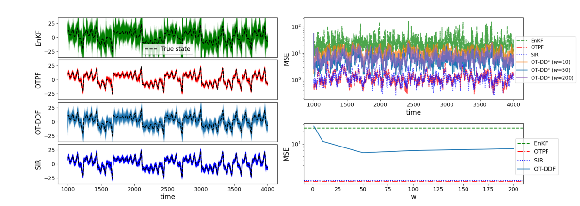
Figure 3: Numerical results for the Lorenz 63 example. The left column shows the trajectory of one of the unobserved components of the particles along with the trajectory of the true state, where $w=50$ for the OT-DDF method (the other components exhibit similar behavior). The right column shows the MSE, in estimating the true state, as a function of time in the upper corner and as a function of the window size $w$ in the lower corner.

IV-C Lorenz 63

We repeated our experiments on a discrete-time (with time-discretization step-size $\Delta t=0.01$) chaotic Lorenz 63 model [25] with the observation function $h(x)=x(1)$ with additive zero-mean Gaussian noise of variance $10^{-1}$. Algorithm 1 was implemented for window sizes $w=10,50,200$ and burn-in time of $t_{0}=1000-w$. The functions $f$ and $T$ wereparameterized with ResNets of hidden size $32$, with learning rate of $10^{-3}$ and $5\times 10^{-3}$, number of iterations $k_{inner}=10$ and $k_{outer}=15000$.

The numerical results are presented in Figure 3. The left panel shows the trajectory of the particles and the true state (only the second component is shown). The right column shows the MSE of estimating the true state, averaged over $10$ independent simulations, as a function of time in the top and as a function of the window size in the bottom. The performance of the OT-DDF filter is expected to improve with further fine-tuning, increasing the iteration number of training and the number of parameters in the neural net.

We also report the wall-clock complexity of all algorithms in Table I. The simulations are carried out on a MAC STUDIO M2 Max with a 12‑core CPU, 30‑core GPU, and 64GB unified memory. The offline training time for the OT-DDF with window size $w=50$ is $46.29$ seconds. The computational time per one-time step update for all methods appears in Table I. The time complexity of all methods except the OTPF algorithm is at the same level of magnitude, which allows the OT-DDF algorithm to be implemented in an online setting once we have access to the map $\hat{T}^{\mu}_{w,0}$. The online time complexity of OT-DDF may be further reduced with the application of neural net compression techniques and parallel processing of particles.

TABLE I: The time complexity for one-time step.

Method	EnKF	SIR	OTPF	OT-DDF
time	$1.7\times 10^{-4}$	$2.0\times 10^{-4}$	$6.8\times 10^{-2}$	$1.5\times 10^{-4}$

V Discussion

We introduced OT-DDF, a completely data-driven nonlinear filtering algorithm applicable to models that admit stationary processes and stable filters. The method provides significant improvement to the original OTPF method in terms of computational cost by limiting the costly training of an OT map to an offline stage using recorded data leading to very fast computations during online inference. Preliminary error analysis and numerical experiments show that in comparison to OTPF, the loss in accuracy is not significant when the window size is chosen properly, and the optimization problem is solved to a reasonable accuracy. Future work will aim to refine the error analysis further and explore the algorithm’s scalability and adaptability to a wider range of applications.

References

- [1] Mohammad Al-Jarrah, Bamdad Hosseini, and Amirhossein Taghvaei. Optimal transport particle filters. In 2023 62nd IEEE Conference on Decision and Control (CDC), pages 6798–6805. IEEE, 2023.
- [2] Mohammad Al-Jarrah, Niyizhen Jin, Bamdad Hosseini, and Amirhossein Taghvaei. Optimal transport-based nonlinear filtering in high-dimensional settings. arXiv preprint arXiv:2310.13886, 2023.
- [3] Ricardo Baptista, Bamdad Hosseini, Nikola B Kovachki, Youssef M Marzouk, and Amir Sagiv. An approximation theory framework for measure-transport sampling algorithms. arXiv preprint arXiv:2302.13965, 2023.
- [4] Yaakov Bar-Shalom, X Rong Li, and Thiagalingam Kirubarajan. Estimation with applications to tracking and navigation: theory algorithms and software. John Wiley & Sons, 2004.
- [5] Thomas Bengtsson, Peter Bickel, and Bo Li. Curse-of-dimensionality revisited: Collapse of the particle filter in very large scale systems. In Probability and statistics: Essays in honor of David A. Freedman, volume 2, pages 316–335. Institute of Mathematical Statistics, 2008.
- [6] Peter Bickel, Bo Li, Thomas Bengtsson, et al. Sharp failure rates for the bootstrap particle filter in high dimensions. In Pushing the limits of contemporary statistics: Contributions in honor of Jayanta K. Ghosh, pages 318–329. Institute of Mathematical Statistics, 2008.
- [7] Edoardo Calvello, Sebastian Reich, and Andrew M Stuart. Ensemble Kalman methods: a mean field perspective. arXiv preprint arXiv:2209.11371, 2022.
- [8] Olivier Cappé, Eric Moulines, and Tobias Rydén. Inference in hidden Markov models. In Proceedings of EUSFLAT Conference, pages 14–16, 2009.
- [9] Guillaume Carlier, Victor Chernozhukov, and Alfred Galichon. Vector quantile regression: an optimal transport approach. The Annals of Statistics, 44(3):1165–1192, 2016.
- [10] Dan Crisan and Boris Rozovskii. The Oxford handbook of nonlinear filtering. Oxford University Press, 2011.
- [11] Fred Daum, Jim Huang, and Arjang Noushin. Exact particle flow for nonlinear filters. In Signal processing, sensor fusion, and target recognition XIX, volume 7697, pages 92–110. SPIE, 2010.
- [12] Flávio Eler De Melo, Simon Maskell, Matteo Fasiolo, and Fred Daum. Stochastic particle flow for nonlinear high-dimensional filtering problems. arXiv preprint arXiv:1511.01448, 2015.
- [13] Pierre Del Moral and Alice Guionnet. On the stability of interacting processes with applications to filtering and genetic algorithms. In Annales de l’Institut Henri Poincaré (B) Probability and Statistics, volume 37, pages 155–194. Elsevier, 2001.
- [14] Vincent Divol, Jonathan Niles-Weed, and Aram-Alexandre Pooladian. Optimal transport map estimation in general function spaces. arXiv preprint arXiv:2212.03722, 2022.
- [15] Arnaud Doucet and Adam M Johansen. A tutorial on particle filtering and smoothing: Fifteen years later. Handbook of nonlinear filtering, 12(3):656–704, 2009.
- [16] Geir Evensen. The ensemble Kalman filter: Theoretical formulation and practical implementation. Ocean dynamics, 53(4):343–367, 2003.
- [17] Geir Evensen. Data Assimilation: The Ensemble Kalman Filter, volume 2. Springer, 2009.
- [18] Neil J Gordon, David J Salmond, and Adrian FM Smith. Novel approach to nonlinear/non-Gaussian Bayesian state estimation. In IEE proceedings F (radar and signal processing), volume 140, pages 107–113. IET, 1993.
- [19] Daniel Grange, Mohammad Al-Jarrah, Ricardo Baptista, Amirhossein Taghvaei, Tryphon T Georgiou, Sean Phillips, and Allen Tannenbaum. Computational optimal transport and filtering on Riemannian manifolds. IEEE Control Systems Letters, 2023.
- [20] Arthur Gretton, Karsten Borgwardt, Malte Rasch, Bernhard Schölkopf, and Alex Smola. A kernel method for the two-sample-problem. Advances in neural information processing systems, 19, 2006.
- [21] Bamdad Hosseini, Alexander W Hsu, and Amirhossein Taghvaei. Conditional optimal transport on function spaces. arXiv preprint arXiv:2311.05672, 2023.
- [22] Rudolph Emil Kalman. A new approach to linear filtering and prediction problems. 1960.
- [23] Jin W Kim and Prashant G Mehta. Duality for nonlinear filtering i: Observability. IEEE Transactions on Automatic Control, 2023.
- [24] Nikola Kovachki, Ricardo Baptista, Bamdad Hosseini, and Youssef Marzouk. Conditional sampling with monotone GANs: from generative models to likelihood-free inference. arXiv preprint arXiv:2006.06755, 2023.
- [25] Edward N Lorenz. Deterministic nonperiodic flow. Journal of atmospheric sciences, 20(2):130–141, 1963.
- [26] Youssef Marzouk, Tarek Moselhy, Matthew Parno, and Alessio Spantini. Sampling via measure transport: An introduction, in Handbook of Uncertainty Quantification. Springer, pages 1–41, 2016.
- [27] Patrick Rebeschini and Ramon Van Handel. Can local particle filters beat the curse of dimensionality? The Annals of Applied Probability, 25(5):2809–2866, 2015.
- [28] Sebastian Reich. A nonparametric ensemble transform method for Bayesian inference. SIAM Journal on Scientific Computing, 35(4):A2013–A2024, 2013.
- [29] Yuyang Shi, Valentin De Bortoli, George Deligiannidis, and Arnaud Doucet. Conditional simulation using diffusion Schrödinger bridges. In Uncertainty in Artificial Intelligence, pages 1792–1802. PMLR, 2022.
- [30] Alessio Spantini, Ricardo Baptista, and Youssef Marzouk. Coupling techniques for nonlinear ensemble filtering. SIAM Review, 64(4):921–953, 2022.
- [31] Amirhossein Taghvaei and Bamdad Hosseini. An optimal transport formulation of Bayes’ law for nonlinear filtering algorithms. In 2022 IEEE 61st Conference on Decision and Control (CDC), pages 6608–6613. IEEE, 2022.
- [32] Amirhossein Taghvaei and Prashant G Mehta. A survey of feedback particle filter and related controlled interacting particle systems (CIPS). Annual Reviews in Control, 2023.
- [33] Ramon Van Handel. Observability and nonlinear filtering. Probability theory and related fields, 145:35–74, 2009.
- [34] Ramon Van Handel. Uniform observability of hidden Markov models and filter stability for unstable signals. 2009.
- [35] Cédric Villani. Topics in optimal transportation. Number 58. American Mathematical Soc., 2003.
- [36] Tao Yang, Richard S Laugesen, Prashant G Mehta, and Sean P Meyn. Multivariable feedback particle filter. Automatica, 71:10–23, 2016.
- [37] Tao Yang, Prashant G Mehta, and Sean P Meyn. Feedback particle filter. IEEE transactions on Automatic control, 58(10):2465–2480, 2013.