Uncertainty Propagation in Stochastic Systems via Mixture Models
with Error Quantification

Abstract

Uncertainty propagation in non-linear dynamical systems has become a key problem in various fields including control theory and machine learning. In this work we focus on discrete-time non-linear stochastic dynamical systems. We present a novel approach to approximate the distribution of the system over a given finite time horizon with a mixture of distributions. The key novelty of our approach is that it not only provides tractable approximations for the distribution of a non-linear stochastic system, but also comes with formal guarantees of correctness. In particular, we consider the total variation (TV) distance to quantify the distance between two distributions and derive an upper bound on the TV between the distribution of the original system and the approximating mixture distribution derived with our framework. We show that in various cases of interest, including in the case of Gaussian noise, the resulting bound can be efficiently computed in closed form. This allows us to quantify the correctness of the approximation and to optimize the parameters of the resulting mixture distribution to minimize such distance. The effectiveness of our approach is illustrated on several benchmarks from the control community.

I Introduction

Modern autonomous systems are becoming increasingly complex, commonly including non-linearities, data-driven components, and uncertain dynamics [1, 2]. The uncertainty affecting these systems can come from various sources including: inherent probabilistic dynamics, lack of knowledge on parts of the model, and interactions with an uncertain environment [1]. Consequently, when autonomous systems need to be employed for safety-critical applications, where failure may translate into costly or deadly accidents, it becomes of paramount importance to consider models that include non-linear stochastic dynamics. Unfortunately, for non-linear stochastic dynamical models, the distribution of the system at a given time cannot be computed in closed-form [3]. This leads to the main research question of this paper: Can we develop an efficient framework for uncertainty propagation in non-linear stochastic dynamical systems with formal guarantees of correctness?

Various methods have been proposed to propagate uncertainty in non-linear stochastic systems [1]. These either consider analytical approximation methods, such as Taylor expansions or Stirling’s interpolation [4, 5], to approximate the one step dynamics of the systems, or consider numerical approximation of the various integrals [6, 7] and/or only propagate discrete samples from the system distribution [8, 9]. However, none of these methods comes with error bounds on the aproximation error. An exception is [10], which is however only limited to Gaussian processes with additive noise and can only guarantee that with high probabilities the system trajectories will stay close to the mean. An alternative approach proposed in [11] is to rely on moment matching to propagate the moments of a non-linear stochastic dynamical systems with non-linearities that are either polynomial or trigonometric functions. However, in practice it is often required to propagate the full distribution, and not just the moments, e.g., for chance constraint satisfaction in planning problems [2]. Additionally, we should stress that, because of their universal approximation properties, various papers already attempted to use mixture distributions, and Gaussian Mixture Models (GMMs) in particular, to approximate the distribution of a stochastic dynamical system [12, 13]. However, these works are mostly based on heuristics on how to build the mixture and come with no guarantees of correctness.

In this work, given an error threshold $\epsilon>0$ and a time horizon $T,$ we develop a framework that for each time step $t\leq T$ builds a mixture distribution approximation of a given non-linear stochastic dynamical system, which is guaranteed to be $\epsilon-$close to the distribution of the system at that time. To quantify the closeness between two distributions we consider the total variation (TV) distance, defined as the largest absolute difference between the probabilities that two probability distributions assign to an event [14]. Interestingly, we show that by appropriately picking the components of the approximating mixture distribution its TV from the unknown distribution of the system at time $t$ can be computed in closed form. For instance, in the case of a stochastic dynamical systems with Gaussian noise (and non-linear dynamics), our framework returns a Gaussian mixture model, whose TV from the unknown true system distribution can be computed in closed form. Using this bound, we then propose a refinement algorithm that iteratively builds mixture models by efficiently placing distributions in regions of the state space by minimizing the TV bound. We empirically illustrate the efficacy of our framework in various benchmarks.

In summary the main contributions of this work are: i) a novel framework for computing a mixture distribution approximating the distribution of a stochastic dynamical systems at a given time, ii) formal bounds of correctness in terms of the TV distance and a proof of convergence of the approximating error to $0$, iii) an adaptive grid refinement algorithm for bound optimization, and iv) empirical evaluation of the efficacy of our framework on four case studies including a Dubin’s car model and an application on a planning problem.

II Problem Formulation

II-A Notation

Given a Borel measurable space $\mathcal{X}\subseteq\mathbb{R}^{q}$ we denote by $\mathcal{P}(\mathcal{X})$ the set of probability distributions on $\mathcal{X}$. For a random variable $x_{t}$ taking values in $\mathcal{X}$, we denote by $\mathbb{P}_{x_{t}}\in\mathcal{P}(\mathcal{X})$ the probability measure associated to $x_{t}$, and by $p_{x_{t}}$ the probability density function associated to $\mathbb{P}_{x_{t}}$. For all the probability distributions considered in this paper, we always assume that they have a density. Additionally, given a set of $K$ probability distributions $\mathbb{P}_{\theta_{1}},...,\mathbb{P}_{\theta_{K}}\in\mathcal{P}(\mathcal{X})$ and a set of weights $\omega_{1},...,\omega_{K}\in[0,1]$ such that $\sum_{k=1}^{K}\omega_{k}=1$, we define a mixture distribution of size $K>0$ as the distribution $\hat{\mathbb{P}}=\sum_{k=1}^{K}\omega_{k}\mathbb{P}_{\theta_{k}}$. If each $\mathbb{P}_{\theta_{k}}$ is a Gaussian distribution, then $\hat{\mathbb{P}}$ is called a Gaussian mixture model (GMM) or Gaussian mixture distribution. Finally, for a probability distribution ${\mathbb{P}}\in\mathcal{P}(\mathcal{X})$ and a measurable function $g:\mathcal{X}\rightarrow\mathcal{Y}$, where $\mathcal{Y}\subseteq\mathbb{R}^{d}$, we denote the push-forward measure of ${\mathbb{P}}$ by $g$ as $g\#{\mathbb{P}}$ such that for all $A\subset\mathcal{Y}$, $(g\#\mathbb{P})(A):=\mathbb{P}(g^{-1}(A))$. We note that $g\#\mathbb{P}$ is still a probability distribution such that $g\#\mathbb{P}\in\mathcal{P}(\mathcal{Y})$.

II-B System Description

We consider a discrete-time stochastic process described by the following stochastic difference equation

$${x}_{t+1}=g({x}_{t},{\varepsilon}_{t})\text{,}\qquad{x}_{0}\sim\mathbb{P}_{x_{0}},\,{\varepsilon}_{t}\sim\mathbb{P}_{{\varepsilon}},$$ (1)

where $g:\mathbb{R}^{d}\times\mathbb{R}^{q}\rightarrow\mathbb{R}^{d}$ is a possibly non-linear continuous function representing the one step dynamics of System (1), $x_{0}$ is a random initial condition with distribution $\mathbb{P}_{x_{0}}\in\mathcal{P}(\mathbb{R}^{d})$, and ${\varepsilon}_{t}$ is a noise term distributed according to a absolutely continuous distribution independent and identically distributed at each time step $\mathbb{P}_{{\varepsilon}}\in\mathcal{P}(\mathbb{R}^{q})$. Intuitively, System (1) represents a general model of a $d-$dimensional discrete-time stochastic system with possible non-linearities both in the state and noise.

In order to study the time evolution of System (1), we first introduce $\mathbb{T}_{x}$, the one-step transition kernel of System (1), which for any time $t$ represents the probability distribution of $x_{t}$ given that $x_{t-1}=x$ and is formally defined as:

$$\mathbb{T}_{x}={g}({x},\cdot)\#\mathbb{P}_{{\varepsilon}}.$$

For simplicity, with an abuse of notation, we denote by $p(y\mid x)$ the probability density associated to $\mathbb{T}_{x}$.

Example 1.

In the case where $g(x,\varepsilon)=f(x)+\varepsilon$ and the noise distribution is $\mathbb{P}_{{\varepsilon}}=\mathcal{N}({0},\Sigma_{{\varepsilon}})$, that is, a zero mean Gaussian with covariance matrix $\Sigma_{{\varepsilon}}$, we have that $\mathbb{T}_{x}=\mathcal{N}(f({x}),\Sigma_{{\varepsilon}})$, a Gaussian distribution with mean $f(x)$ and covariance matrix $\Sigma_{{\varepsilon}}$.

The probability distribution of System (1) at time $t$, $\mathbb{P}_{x_{t}}$, can be described by its density $p_{{x}_{t}},$ which can be computed iteratively over time by using the following Chapman-Kolmogorov equation [3, 12]:

$$p_{x_{t}}(y)=\int_{\mathbb{R}^{d}}p(y\mid x)p_{x_{t-1}}(x)dx.$$ (2)

That is, $p_{{x}_{t}}$ is obtained by marginalizing the one-step transition kernel w.r.t. $p_{{x}_{t-1}}.$ Unfortunately, even though $p(y\mid x)$ can be expressed in closed form in many cases of interest, Eqn (2) is in general not tractable. For instance, this is the case for the system in Example 1 where $p(y\mid x)$ is Gaussian, but $p_{x_{t}}$ is intractable and non-Gaussian if $f$ is non-linear. Consequently, approximation schemes are required.

II-C Problem Statement

Our goal in this paper is to design an approximating mixture distribution $\hat{\mathbb{P}}_{x_{t}}$, which is close to the actual probability distribution $\mathbb{P}_{x_{t}}$, but that is also tractable and can be computed analytically in closed form. To do that, we need to introduce a metric to quantify the distance between probability distributions. While many metrics have been introduced for this task [14], in this paper we focus on the Total Variation (TV) distance.

Definition 1 (Total Variation).

Let $(\mathcal{X},\mathcal{B}(\mathcal{X}))$ be a measurable space, and $\mathbb{P},\mathbb{Q}\in\mathcal{P}(\mathcal{X})$ be probability distributions. Then, the Total Variation (TV) distance between $\mathbb{P}$ and $\mathbb{Q}$ is defined as:

$$\text{TV}(\mathbb{P},\mathbb{Q}):=\sup_{A\in\mathcal{B}(\mathcal{X})}|\mathbb{P}(A)-\mathbb{Q}(A)|.$$

Intuitively, the TV is the largest difference that the probability of the same event can have according to two probability distributions. Consequently, because of its intuitive and worst case nature, the TV represents a particularly convenient choice to quantify the distance between the distribution of stochastic dynamical systems. We should also stress that, differently from the TV case, closeness in other measures commonly employed, such as Wasserstein distance, does not necessarily imply closeness in the probability of events [14].

We are finally ready to formulate our problem statement.

Problem 1.

Consider a finite time horizon $\{1,...,T\}\subset\mathbb{N}$, and a threshold $\delta>0.$ Find a set of mixture distributions of finite size $\hat{\mathbb{P}}_{x_{1}},...,\hat{\mathbb{P}}_{x_{T}}$ such that for all $t\in\{1,...,T\}$ it holds that:

$$\text{TV}\left(\mathbb{P}_{x_{t}},\hat{\mathbb{P}}_{x_{t}}\right)\leq\delta.$$ (3)

Note that Problem 1 is stated for a general mixture distribution $\hat{\mathbb{P}}_{x_{t}}$. This is because depending on the one-step transition kernel of System (1), one may want to focus on different classes of mixture distributions. Nevertheless, because of their modelling flexibility and because of the existence of TV bounds between two Gaussian distributions [15], in this paper we will give particular attention to GMMs.

We should also note that solving Problem 1 is particularly challenging not only because Eqn (2) cannot be solved in closed form, but also because it requires to propagate over time the uncertainty introduced by each approximation step. In fact, according to Eqn (2), to compute $\mathbb{P}_{x_{t}}$, one needs to marginalize the one step transition kernel wrt $\mathbb{P}_{x_{t-1}},$ which is unknown for any $t>0$.

Approach

To solve Problem 1, we propose a stochastic approximation scheme consisting of an iterative process based on approximation of Eqn (2) with a mixture distribution. Intuitively, we partition $\mathbb{R}^{d}$ in various subspaces $\mathcal{X}_{k}$ and select representative points $x^{(k)}\in\mathcal{X}_{k}$ such that $\int_{\mathbb{R}^{d}}p(y\mid x)p_{x_{t}}(x)dx$ is close to $\sum_{k=1}^{K}p(y\mid x^{(k)})\int_{\mathcal{X}_{k}}p_{x_{t}}(x)dx$. In Section III, we detail our stochastic approximation scheme, and we state proof its correctness and convergence to the distribution of System (1). In Section IV, we present the resulting algorithm used to build the mixture approximations. Finally, in Section V, we present numerical experiments.

III Stochastic Approximation Scheme

To solve Problem 1, we introduce a stochastic approximation scheme based on iteratively approximating the distribution of System (1) by mixtures of the one-step transition kernel. In particular, for each time step $t$ we consider a partition of $\mathbb{R}^{d}$ in $K_{t}$ non-overlapping regions $\bm{\mathcal{X}}_{t}:=\{\mathcal{X}^{(1)}_{t},...,\mathcal{X}^{(K_{t})}_{t}\}$ and for each $\mathcal{X}^{(k)}_{t}\in\bm{\mathcal{X}}_{t}$ we consider a representative point $x^{(k)}_{t}\in\mathcal{X}^{(k)}_{t}.$ Then, we define the approximating mixture distribution $\hat{\mathbb{P}}_{x_{t}}$ iteratively as follows:

$$\hat{\mathbb{P}}_{x_{0}}:=\mathbb{P}_{x_{0}}$$

$$\hat{\mathbb{P}}_{x_{t}}:=\sum_{k=1}^{K_{t-1}}\omega^{(k)}_{t}{\mathbb{T}}_{x^{(k)}_{t-1}}$$ (4)

with $\omega^{(k)}_{t}:=\hat{\mathbb{P}}_{x_{t-1}}({\mathcal{X}^{(k)}_{t-1}}).$ Intuitively, at each time $t$, Eqn (4) builds a mixture approximation of $\mathbb{P}_{x_{t}}$ by averaging the one-step transition kernel of System (1) with weights that depend on the approximating mixture distribution at the previous time step.

Example 2.

For the system dynamics of Example 1, Eqn (4) leads to a mixture distribution approximation at time step $t$ given by the GMM $\hat{\mathbb{P}}_{x_{t}}=\sum_{k=1}^{K_{t-1}}\omega^{(k)}_{t}\mathcal{N}(f(x^{(k)}_{t-1}),\Sigma_{\varepsilon})$, where $\omega^{(k)}_{t}=\hat{\mathbb{P}}_{x_{t-1}}({\mathcal{X}^{(k)}_{t-1}})$ is the probability mass of the GMM $\hat{\mathbb{P}}_{x_{t-1}}=\sum_{k=1}^{K_{t-2}}\omega^{(k)}_{t-1}\mathcal{N}(f(x^{(k)}_{t-2}),\Sigma_{\varepsilon})$ (built in the previous step) within the region $\mathcal{X}^{(k)}_{t-1}$.

Remark 1.

Note that the mixture $\hat{\mathbb{P}}_{x_{t}}$ as defined in Eqn (4) is not necessarily a Gaussian mixture. If for the particular application it would be preferable to obtain a GMM, then this can always be obtained by approximating each ${\mathbb{T}}_{x^{(k)}_{t-1}}$ in Eqn (4) with a Gaussian (mixture) distribution. As the total variation is a distance that satisfies the triangle inequality, then the bounds on the approximation error developed in the rest of this section would hold also for this setting, with a correction term depending on the closeness of each ${\mathbb{T}}_{x^{(k)}_{t-1}}$ to the respective Gaussian or Gaussian mixture approximation.

It is obvious that the quality of the approximation obtained from Eqn (4) depends on the choice of the weights and representative points. How to perform this choice is the object of Section IV. In the remainder of this section, we focus on quantifying $\text{TV}(\hat{\mathbb{P}}_{x_{t}},{\mathbb{P}}_{x_{t}})$.

III-A Total variation bounds

We start our analysis with Theorem 1, where we bound $\text{TV}(\hat{\mathbb{P}}_{x_{t}},{\mathbb{P}}_{x_{t}})$. Proofs for Theorems and Lemmas of this Section can be found in the Section VI.

Theorem 1.

Let function $s\big{(}x,x^{(k)}\big{)}$ be defined as

$$s\big{(}x,x^{(k)}\big{)}:=\frac{1}{2}\int_{\mathbb{R}^{d}}\big{|}p(y\mid x)-p(y\mid x^{(k)})\big{|}dy$$ (5)

Then, for any $t>0$ it holds that

$$\begin{split}&\text{TV}\left(\mathbb{P}_{x_{t}},\hat{\mathbb{P}}_{x_{t}}\right)\leq\text{TV}\left(\mathbb{P}_{x_{t-1}},\hat{\mathbb{P}}_{x_{t-1}}\right)+\\ &\qquad\sum_{k=1}^{K_{t-1}}\max_{{x}\in\mathcal{X}^{(k)}_{t-1}}s\big{(}{x},x^{(k)}_{t-1}\big{)}\hat{\mathbb{P}}_{x_{t-1}}(\mathcal{X}^{(k)}_{t-1}),\end{split}$$ (6)

where $\text{TV}\left(\mathbb{P}_{x_{0}},\hat{\mathbb{P}}_{x_{0}}\right)=0$.

Theorem 1 guarantees that the approximation error at each time step propagates at most linearly over time. Furthermore, because of term $\hat{\mathbb{P}}_{x_{t-1}}(\mathcal{X}^{(k)}_{t-1})$, only regions with non-negligible probability mass w.r.t. $\hat{\mathbb{P}}_{x_{t-1}}$ influence the TV bound. The key component of Theorem 1 is function $s\big{(}{x},x^{(k)}_{t-1}\big{)}$, which is equivalent to $\text{TV}(\mathbb{T}_{x},\mathbb{T}_{x^{(k)}_{t-1}})$, i.e., the total variation between the one-step transition kernel at $x$ and $x^{(k)}_{t-1}$. Consequently, the computation of $s\big{(}{x},x^{(k)}_{t-1}\big{)}$ depends on the specific noise distribution in System (1).

Luckily, closed form expressions for $s\big{(}{x},x^{(k)}_{t-1}\big{)}$ or for upper bounds exists for many cases of interest, including when $\mathbb{T}_{x}$ follows a Gaussian, Gamma, or uniform distribution. Because of its widespread use, the Gaussian case is explicitly considered in detail in the next paragraph. For the Gamma distribution one can use the fact that $s$ can be bounded by the KL divergence using Pinsker’s inequality and then rely on closed forms for the KL divergence between Gamma distributions [16]. For the uniform distribution, computing $s$ can be performed by separating the integral in regions based on the overlapping of the supports (which can be easily done when the dimensions are independent, and hence the supports are hyper-rectangles).

Total Variation Bounds for the Gaussian Case

The following result is a corollary of Theorem 1 in the case of additive Gaussian noise.

Corollary 1.

Assume that $g(x_{t},\bm{\varepsilon}_{t})=f(x_{t})+\bm{\varepsilon}_{t}$ and $\bm{\varepsilon}_{t}\sim\mathcal{N}(0,\Sigma_{\varepsilon})$. Then, for any $t>0$ it holds that

$$\begin{split}&\text{TV}\left(\mathbb{P}_{x_{t}},\hat{\mathbb{P}}_{x_{t}}\right)\leq\text{TV}\left(\mathbb{P}_{x_{t-1}},\hat{\mathbb{P}}_{x_{t-1}}\right)+\\ &\qquad\sum_{k=1}^{K_{t-1}}\text{erf}\left(\max_{{x}\in\mathcal{X}^{(k)}_{t-1}}h\big{(}{x},x^{(k)}_{t-1}\big{)}\right)\hat{\mathbb{P}}_{x_{t-1}}(\mathcal{X}^{(k)}_{t-1}),\end{split}$$ (7)

where $\text{TV}\left(\mathbb{P}_{x_{0}},\hat{\mathbb{P}}_{x_{0}}\right)=0$ and

$$h\big{(}x,x^{(k)}_{t-1}\big{)}:=\frac{1}{2\sqrt{2}}\sqrt{(f\left(x\right)-f(x^{(k)}_{t-1}))^{T}\Sigma_{\varepsilon}^{-1}(f(x)-f(x^{(k)}_{t-1}))}.$$

Eqn (7) follows from Theorem 1 using the fact that when the one-step transition kernel is Gaussian, then $s\big{(}x,x^{(k)}_{t-1}\big{)}$ can be computed in a closed form in terms of the function $h\big{(}x,x^{(k)}_{t-1}\big{)}$. Note also that for any $x\in\mathcal{X}_{t-1}^{(k)}$ the function $h\big{(}x,x^{(k)}_{t-1}\big{)}$, and consequently the tightness of the bounds, depends on the following factors: (i) $f(x)-f(x^{(k)}_{t-1})$, which quantifies how much $f$ varies locally, (ii) $\Sigma_{\varepsilon}^{-1}$, which suggests that lower noise variances may lead to worse bounds. This should not appear surprising, when considering the definition of TV in Definition 1. In fact, from the definition of TV it follows that the TV between two delta Dirac distributions is zero unless they have exactly the same mean. Consequently, the smaller the noise variance, the more local variation of $f(x)$ from the mean of each component of the GMM will affect the bound.

Remark 2.

Corollary 1 can be straightforwardly generalized to the case where the covariance matrix varies with time, as long as it is independent of $x$. If heteroscedasticity is required in the noise model, one possible strategy is to adapt the proof using the fact that KL divergence can be used to upper bound the TV distance and use Prop. 2.1 of [15] to bound term $s$.

For both Theorem 1 and Corollary 1, at each time step the TV bound is obtained by a sum over all components in the mixture. An interesting question is whether the bound decreases with a mixture of larger size. We answer positively to this question in the following subsection, where we prove the convergence of our method: the $\text{TV}\left(\mathbb{P}_{x_{t}},\hat{\mathbb{P}}_{x_{t}}\right)$ goes to zero for approximating mixture models of arbitrarily large size.

III-B Convergence Analysis

In Theorem 2 below we show that the approximation error introduced by Eqn (4) can be made arbitrarily small by increasing the size of the mixture.

Theorem 2.

For $\bar{x}\in\mathbb{R}^{d}$ assume that $\mathbb{T}_{\bar{x}}$-almost surely (a.s.) for every $y\in\mathbb{R}^{d}$ it holds that

$$\|x-\bar{x}\|_{\infty}\rightarrow 0\implies p(y\mid x)\rightarrow p(y\mid\bar{x}),$$

where $\|x-\bar{x}\|_{\infty}$ is the infinity norm of vector $x-\bar{x}.$ Then, for any $\epsilon>0$ and any time $t<\infty$, there exists a sequence of partitions $\{\bm{\mathcal{X}}_{0},...,\bm{\mathcal{X}}_{t-1}\}$ such that

$$\text{TV}\left(\mathbb{P}_{t},\hat{\mathbb{P}}_{t}\right)\leq\epsilon.$$ (8)

Note that the assumption of almost surely continuity of $p(y\mid x)$ in Theorem 2 is not particularly restrictive. For instance, it holds for distributions with continuous density, e.g., Gaussian, or even with bounded support, where the boundary of the support has measure zero.

Remark 3.

We should remark that the convergence in Theorem 2 is proved assuming that each $\bm{\mathcal{X}}_{i}$ is a uniform partition of a compact set containing $1-\frac{\epsilon}{2t}$ probability mass of $\hat{\mathbb{P}}_{x_{i}}.$ While sufficient for showing convergence, this choice of partition is obviously sub-optimal, as in general we would like to place more distributions from the mixture in regions where there is more probability mass. This is explored in our algorithmic framework detailed in the next section.

IV Algorithm

We summarize our overall procedure to solve Problem 1 in Algorithm 1. For every time $t,$ in Lines 2-5 we compute the approximating mixture at the current time step following Eqn (4). Then, in Line 6 we identify a hyper-rectangle $\mathcal{S}_{t}$ containing at least $1-\epsilon$ probability mass of $\hat{\mathbb{P}}_{x_{t}}$, where $\epsilon$ is a given parameter, which in our implementation, for time step $t$ is taken as $\epsilon\ll\frac{\delta}{T}$, such that the impact of not partitioning region $\mathbb{R}^{d}\setminus\mathcal{S}_{t}$ on the bound is small compared to our desired precision. Such a region can either be identified analytically as $\hat{\mathbb{P}}_{x_{t}}$ is known, e.g., in the case $\hat{\mathbb{P}}_{x_{t}}$ is a GMM, or using samples. $\mathcal{S}_{t}$ is then partitioned in an initial set of $K_{t}$ hyper-rectangles in Line 7 such that all regions contain (approximately) probability $p_{\text{thr}}$ (a parameter usually set to $1\%$ in our experiments) by iteratively cutting the axis in half and checking the inside probability until the threshold is met. This allows us to segment initial regions by probability mass (see left grid in Figure 1), and not by size, as it is the case with uniform/equidistant grids. We encode the resulting set of representative points corresponding to partition $\bm{\mathcal{X}}_{t}:=\{\mathcal{X}^{(1)}_{t},...,\mathcal{X}^{(K_{t})}_{t}\}$ by $\bm{x}^{\text{repres}}_{t}:=\{x^{(1)}_{t},...,x^{(K_{t})}_{t}\}$ and for each $\mathcal{X}^{(k)}_{t}$ we select $x^{(k)}_{t}$ as its center point. The resulting grid is then refined in Lines 10-12 until the TV bound is smaller than a given threshold, $t\frac{\delta}{T}$, with a refinement procedure, which is detailed in subsection IV-A. Note that, because at each time step the TV bound is propagated at the next time step (see Theorem 1), this guarantees that the for each $t\in\{0,...,T\}$ we have that ${TV}(\mathbb{P}_{x_{t}},\hat{\mathbb{P}}_{x_{t}})$ will be smaller than $\delta$. We should also stress that, in practice, the computational complexity of Algorithm 1 is dominated by Step 8, which for each region requires to compute the probability mass of each component of the mixture, thus requiring a total number of integral evaluations quadratic in the size of the mixture (as in general the number of components and regions are close across consecutive iterations).

Input: $\epsilon$, $p_{\text{thr}}$, $\delta$

Output: Mixture approximations $\{\hat{\mathbb{P}}_{x_{t}}\}_{t=1}^{T}$, and TV bounds $\{\text{TV}_{t}\}_{t=1}^{T}$

1

2for $t\in\{0,...,T-1\}$ do

3       if $t=0$ then

4             $\hat{\mathbb{P}}_{x_{0}}\leftarrow\mathbb{P}_{x_{0}}$, $\text{TV}_{0}\leftarrow 0$

5       else

6             $\hat{\mathbb{P}}_{x_{t}}\leftarrow\sum_{k=1}^{K_{t-1}}\omega^{(k)}_{t}{\mathbb{T}}_{x^{(k)}_{t-1}}$

7      $\mathcal{S}_{t}=\texttt{IdentifyHighProbRegion}(\hat{\mathbb{P}}_{x_{t}},\epsilon)$

8      $\bm{\mathcal{X}}_{t},\bm{x}^{\text{repres}}_{t}\leftarrow\texttt{BuildGrid}(\mathcal{S}_{t},p_{\text{thr}})$

9      $\bm{\omega}_{t}\leftarrow\{\hat{\mathbb{P}}_{x_{t}}(\mathcal{X}^{(1)}_{t}),...,\mathbb{P}_{x_{t}}(\mathcal{X}^{(K_{t})}_{t})\}$

10      $\text{TV}_{t+1}\leftarrow\text{TV}(\mathbb{P}_{x_{t+1}},\hat{\mathbb{P}}_{x_{t+1}})\text{ using Thm \ref{thm:general-case}}$

11      while $\text{TV}_{t+1}\geq t\frac{\delta}{T}$ do

12             $\bm{\mathcal{X}}_{t},\bm{x}^{\text{repres}}_{t},\bm{\omega}_{t}\leftarrow\texttt{Refine}(\bm{\mathcal{X}}_{t},\bm{x}^{\text{repres}}_{t},\bm{\omega}_{t})$

13            $\text{TV}_{t+1}\leftarrow\text{TV}(\mathbb{P}_{x_{t+1}},\hat{\mathbb{P}}_{x_{t+1}})\text{ using Thm \ref{thm:general-case}}$

return $\{\hat{\mathbb{P}}_{x_{1}},...,\hat{\mathbb{P}}_{x_{T}}\}$ , $\{\text{TV}_{1},...,\text{TV}_{T}\}$

Algorithm 1 Mixture approximation with TV bounds for $T<\infty$ time steps given an error threshold $\delta$

IV-A Refinement Procedure

The refinement procedure is described in Algorithm 2. The underlying idea of the refinement procedure is to rely on Theorem 1, where we can observe that for any $t$, $\text{TV}(\mathbb{P}_{x_{t}},\hat{\mathbb{P}}_{x_{t}})$ depends on a sum over regions in $\bm{\mathcal{X}}_{t-1}$, where each ${\mathcal{X}^{(k)}}_{t-1}\in\bm{\mathcal{X}}_{t-1}$ contributes to the TV bound with the quantity $\max_{{x}\in\mathcal{X}^{(k)}_{t-1}}s\big{(}{x},x^{(k)}_{t-1}\big{)}\hat{\mathbb{P}}_{x_{t-1}}(\mathcal{X}^{(k)}_{t-1}):=c^{(k)}$. The refinement procedure boils down to partitioning regions whose contribution to the TV bound is high in relative terms. More specifically, if the contribution $c^{(k)}$ of the hypercube $\mathcal{X}^{(k)}$ is higher than a threshold $\gamma>0$, we cut the region in $2^{d}$ subregions by dividing each axis by $2$ in its mid point. An example of a refinement step is illustrated in Figure 1, where we can see that the refinement step decided to cut all inner regions except for the corners.

1

2 function Refine($\bm{\mathcal{X}},\bm{x}^{\text{repres}},\bm{\omega}$):

3       for $\mathcal{X}^{(k)},x^{(k)}$ in $\bm{\mathcal{X}},\bm{x}^{\text{repres}}$ do

4             $c^{(k)}\leftarrow\max_{x\in\mathcal{X}^{(k)}}s\big{(}x,x^{(k)}\big{)}\hat{\mathbb{P}}_{x_{t-1}}\big{(}\mathcal{X}^{(k)}\big{)}$

5            if $c^{(k)}>\gamma$ then

6                   Cut $\mathcal{X}^{(k)}$ in $2^{d}$ hypercubes

7            

8      $\bm{\omega}\leftarrow\{\hat{\mathbb{P}}_{x_{t}}(\mathcal{X}^{(1)}_{\text{new}}),...,\hat{\mathbb{P}}_{x_{t}}(\mathcal{X}^{(K^{*})}_{\text{new}})\}$

9      return $\mathcal{X},\bm{x}^{\text{repres}},\bm{\omega}$

Algorithm 2 Refining the grid

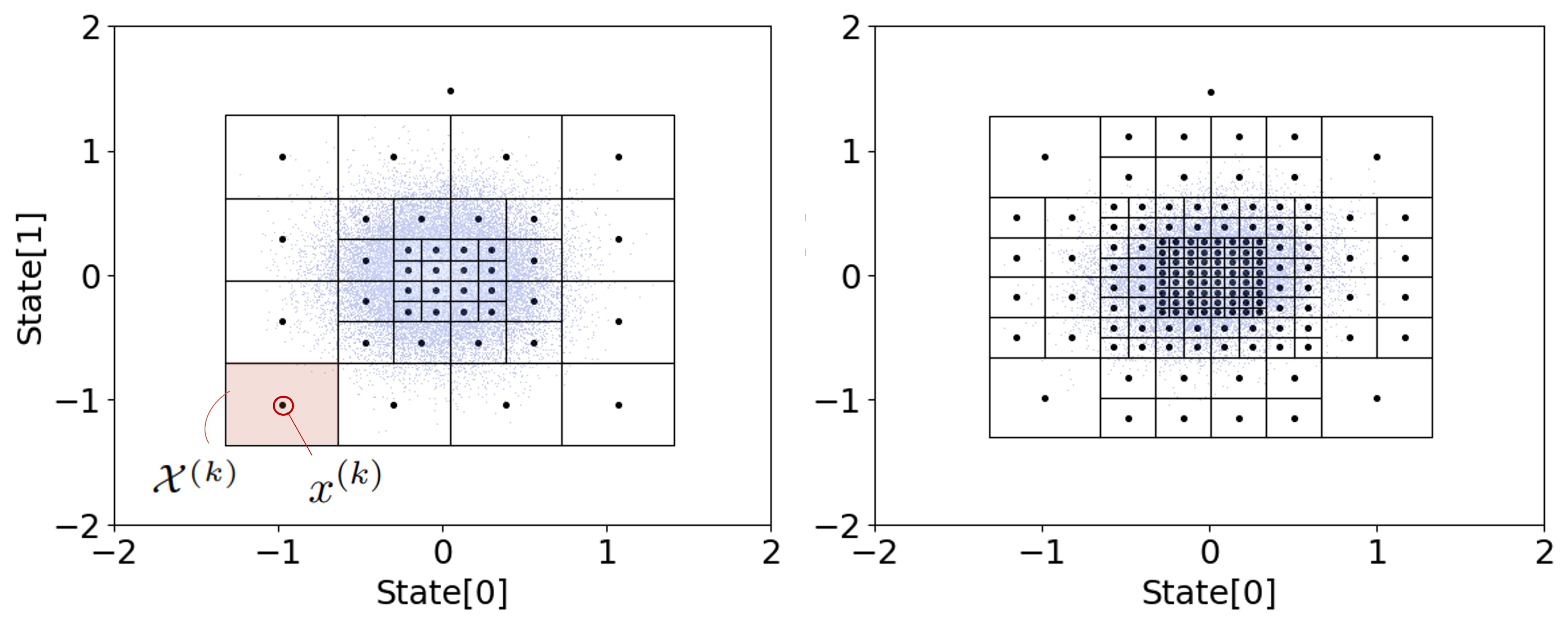
Figure 1: Example of a partition used to propagate the the distribution of the System presented in Example 1 with $\varepsilon\sim\mathcal{N}(0,0.1I)$. The initial grid (left) is refined (right) with a contribution threshold of $\gamma=1\times 10^{-3}$. We see that the algorithm decided to cut all regions except for the corners.

V EXPERIMENTAL RESULTS

For our experiments we consider the following benchmarks:

• A 2-D linear system with bimodal initial distribution with dynamics given by $g(x_{t},\varepsilon_{t})=Ax_{t}+\varepsilon_{t}$, where $A=\begin{bmatrix}0.84&0.10\\ 0.05&0.72\end{bmatrix}$ and $\varepsilon_{t}\sim\mathcal{N}([0,0]^{T},0.03I)$. The initial distribution is a mixture of two Gaussian distributions, that is, $x_{0}\sim 0.5\times\mathcal{N}([6,10]^{T},0.005I)+0.5\times\mathcal{N}([8,10]^{T},0.005I)$.

• A 2-D linear system with dynamics equal to the previous one, but with noise and initial condition following a uniform distribution. Specifically we set $\varepsilon_{t}\sim\mathcal{U}([-0.3,0.3])\times\mathcal{U}([-0.3,0.3])$, that is, a uniform distribution for each component of the noise between $[-0.3,0.3]$. For the initial distribution we assume $x_{0}\sim\mathcal{U}([-0.1,0.1])\times\mathcal{U}([-0.1,0.1])$.

• An unstable polynomial system $g(x_{t},\varepsilon_{t})=f(x_{t})+\varepsilon_{t}$ where $f(x)=[f_{1}(x),f_{2}(x)]^{T}$ with

  $$f_{1}(x) =x_{1}+1.25hx_{2}$$

  $$f_{2}(x) =1.4x_{2}+0.3h(0.25x_{1}^{2}-0.4x_{1}x_{2}+0.25x_{2}^{2})$$

  for $h=0.05$, $\varepsilon_{t}\sim\mathcal{N}([0,0]^{T},\sigma^{2}I)$, where $\sigma\in\{1,0.1,0.001,0.0001\}$ and $x_{0}\sim\mathcal{N}([1,1]^{T},0.002I)$.

• A 3D Dubins car model with constant velocity from [17], with $v=5$, $h=0.3$, and $u=1/0.5$, with $x_{0}\sim\mathcal{N}([0,0,0]^{T},[0.005,0.005,0.001]])$, and $\varepsilon_{t}\sim\mathcal{N}([0,0,0]^{T},[0.06,0.06,0.01])$.

In Algorithm 1, we set $p_{\text{thr}}=0.01$ ($0.001$ for Dubins) to build the initial grid, and for the refinement in Algorithm 2 we choose $\gamma$ ranging from $10^{-6}$ to $10^{-7}$ depending on the case. All experiments were run on an Intel Core i7-1365U CPU with 16GB of RAM. Step 8 of Algorithm 1 was parallelized on 10 cores (given that this step is the bottleneck in terms of computational complexity).

V-A Tightness of the Bounds

We start our analysis from Table I, where we study the efficacy of Algorithm 1 to build a GMM approximation for the polynomial system benchmark. The table shows that unless the variance of the noise, and consequently of the one-step transition kernel, becomes very small (below $10^{-2}$) even a GMM of relatively few mixtures (order of $100$) can obtain relatively tight TV bounds and be employed to solve Problem 1. However, when the variance of the noise becomes small and the noise distribution becomes closer to a delta Dirac, as already discussed right below Corollary 1, obtaining tight TV bounds become harder. Nevertheless, as illustrated in Figure 3, we should stress that, even if obtaining tight TV bounds in this setting becomes more challenging, the distribution obtained with our framework is still empirically very close to the true one even with mixtures of relatively small size.

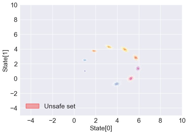
(a) True distribution

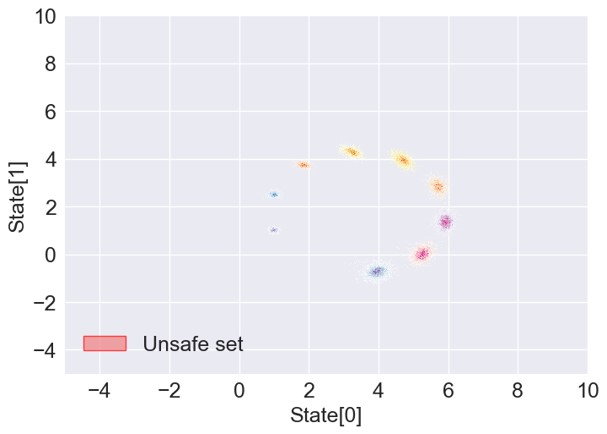
(b) Mixture approximation

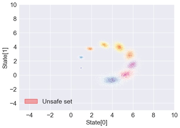
(a) True distribution

(b) Mixture approximation

Figure 3: Upper row considers the Dubins car setting with low noise variance (i.e. $10^{-3}$ for the positions $x_{1}$ and $x_{2}$, and $10^{-4}$ for the steering angle $x_{3}$), while the lower row considers a higher variance noise ($10^{-2}$, and $2\times 10^{-3}$, respectively). The mixtures are generated with only one refinement (see Algorithm 2) with $\gamma=10^{-6}$, resulting in mixtures of size 2500-3000. True distribution means Monte Carlo sampling from the system, while the plots on the right are generated by sampling our mixture distributions.

In Table II we report an empirical evaluation of our approach for all the four benchmarks. For all cases, we consider $5$ refinement steps and compare the mixture model obtained from Algorithm 1 with the standard approach in [1] (called equidistant grid, which we will sometimes refer to uniform grid), where each distribution in the mixture is uniformly spaced in a region containing most of the probability mass of the system and obtained via samples. We consider a time horizon of $T=10$ for the bimodal case, $T=7$ for the polynomial, and $T=5$ for Dubins car and uniform settings. In all cases we can see how Algorithm 2 substantially outperform the approach mentioned in [1] by obtaining much better bounds for an equivalent number of regions. In the Dubins car, for instance, we were not able to obtain informative bounds (e.g. $\ll 1$) for a reasonable number of regions, while Algorithm 2 allowed for bounds between $3\%$ (first time step) to $20\%$ (last).

Noise variance $\sigma^{2}$	$1$		$10^{-1}$		$10^{-2}$		$10^{-3}$
# refinements	TV	GMM size	TV	GMM size	TV	GMM size	TV	GMM size
Initial grid	0.020	121	0.061	124	0.205	115	0.471	127
1	0.011	485	0.031	497	0.107	461	0.279	509
2	0.006	1,937	0.016	1,982	0.054	1,841	0.151	2,033
3	0.003	7,667	0.008	7,868	0.027	7,331	0.078	8,108
4	0.002	26,288	0.005	30,824	0.014	28,997	0.039	32,213
5	0.002	31,070	0.003	59,660	0.007	112,994	0.020	127,220

TABLE I: TV bounds for a 1-time step propagation of the polynomial system for the same initial distribution $x_{0}$ for various values of variance $\sigma^{2}$. In each row we show an iteration of the refinement algorithm and report both the resulting TV bound and the size of the approximating GMM.

	Bimodal		Polynomial		Uniform		Dubins
Grid method	Alg 2	Equid	Alg 2	Equid	Alg 2	Equid	Alg 2	Equid
$\text{TV}_{1}$	0.004	0.007	0.004	0.006	0.004	0.003	0.028	0.99
$\text{TV}_{T}$	0.061	0.092	0.099	0.179	0.041	0.048	0.198	1.00
Avg TV	0.033	0.049	0.039	0.070	0.022	0.022	0.101	1.00

TABLE II: TV bounds for the first and last propagation steps (as well as for the average) for each system. The bounds are computed from grids generated by Algorithm 2 (Alg 2) with 5 refinements and by the uniform/equidistant grids (Equid) of equivalent size.

V-B Application to chance constrained certification

To highlight the usefulness of our approach, we show how it can be employed to quantify the probability that, at each time step, System (1) satisfies probabilistic constraints, a setting commonly occurring in in planning problems for stochastic systems [19, 20, 21]. In particular, for the bimodal system we consider the setting in Figure 4, where the goal is to quantify the probability that at each time step the system will enter the unsafe region in red (which we denote by $p_{\text{hit}}$. In Table III, we report both the empirical value obtained by simulating the specific system $10^{4}$ times and the upper bound of the hitting probability at each time step according to our framework (computed as the probability that the GMM approximation hits the obstacle + the TV bound at the particular time step computed according to Theorem 1). We observe that the upper bound for $p_{\text{hit}}$ is fairly close to the actual hitting probability of the system, due to two factors: i) the hitting probability estimated by our mixture is very close to the true value (analogous to what is shown e.g. in Figure 3), and ii) the TV bounds are reasonably close to zero (see also Table II).

	Bimodal
Time step	Actual hitting probabity $p_{\text{hit}}$	Upper bound $p_{\text{hit}}$
1	0.0	0.4
2	0.0	0.9
3	0.0	1.6
4	0.0	2.4
5	18.4	21.5
6	38.0	42.1
7	20.9	25.6
8	3.5	8.5
9	0.0	5.8
10	0.0	6.2

TABLE III: Actual $p_{\text{hit}}$ is the unsafe set hitting probability computed via Monte Carlo simulation of the actual system ($10^{4}$ samples), while the upper bound is given by the probability mass of the GMM inside the unsafe set + TV bound.

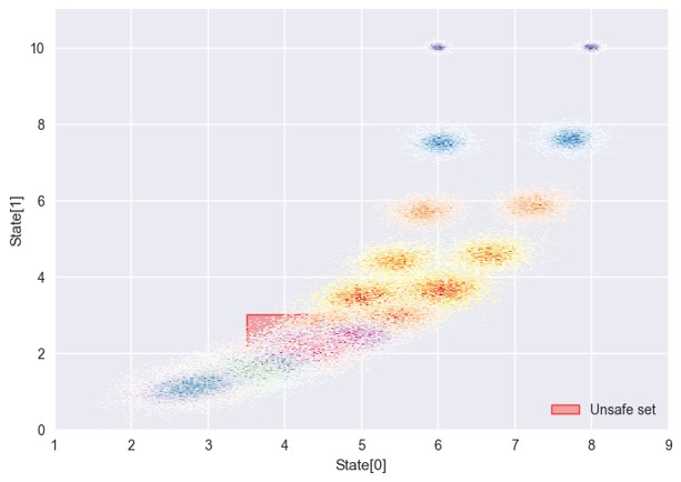
(a) True distribution

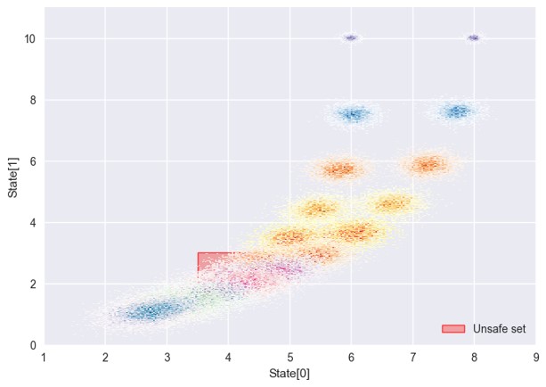
(b) Mixture approximation

Figure 4: Bimodal setting for which we present the hitting probability study. The left image shows a Monte Carlo simulation of the system, while the right displays samples from our mixture approximation. $p_{\text{hit}}$ is computed w.r.t. the red set.

VI PROOFS

VI-A Proof of Theorem 1

For the proof we introduce a new auxiliary distribution $\tilde{\mathbb{P}}_{x_{t}}$, whose density is defined as

$$\tilde{p}_{x_{t}}(y):=\int_{\mathbb{R}^{d}}p(y\mid x)\hat{p}_{x_{t-1}}(x)dx.$$

That is, $\tilde{\mathbb{P}}_{x_{t}}$ is the probability distributions given by the propagation of mixture $\hat{P}_{x_{t-1}}$ through the dynamics of the system. Then, the proof uses the fact that by the triangle inequality

TV $$\left(\mathbb{P}_{x_{t}},\hat{\mathbb{P}}_{x_{t}}\right)\leq\text{TV}\left(\mathbb{P}_{x_{t}},\tilde{\mathbb{P}}_{x_{t}}\right)+\text{TV}\left(\tilde{\mathbb{P}}_{x_{t}},\hat{\mathbb{P}}_{x_{t}}\right).$$

Consequently, to bound $\text{TV}\left(\mathbb{P}_{x_{t}},\hat{\mathbb{P}}_{x_{t}}\right)$ it is enough to bound $\text{TV}\left(\mathbb{P}_{x_{t}},\tilde{\mathbb{P}}_{x_{t}}\right)$ and $\text{TV}\left(\tilde{\mathbb{P}}_{x_{t}},\hat{\mathbb{P}}_{x_{t}}\right).$ We start from $\text{TV}\left(\tilde{\mathbb{P}}_{x_{t}},\hat{\mathbb{P}}_{x_{t}}\right)$. To do that we first note that for every $y\in\mathbb{R}^{d}$, the following holds:

$$|\tilde{p}_{x_{t}}(y) -\hat{p}_{x_{t}}(y)|$$

$$=\Bigl{|}\int_{\mathbb{R}^{d}}p(y\mid x)\hat{p}_{x_{t-1}}(x)dx-\sum_{k=1}^{K_{t-1}}\omega^{(k)}_{t}p(y\mid x^{(k)}_{t-1})\Bigr{|}$$

$$=\Bigl{|}\sum_{k=1}^{K_{t-1}}\int_{\mathcal{X}^{(k)}_{t-1}}\big{(}p(y\mid x)-p(y\mid x^{(k)}_{t-1})\big{)}\hat{p}_{x_{t-1}}(x)dx\Bigr{|}$$

$$\leq\sum_{k=1}^{K_{t-1}}\int_{\mathcal{X}^{(k)}_{t-1}}\big{|}p(y\mid x)-p(y\mid x^{(k)}_{t-1})\big{|}\hat{p}_{x_{t-1}}(x)dx,$$

where the second line uses the definition of $\omega^{(k)}_{t}$ in Eqn (4), and the third the triangle inequality. From this it follows that

$$\begin{split}&\text{TV}\left(\tilde{\mathbb{P}}_{x_{t}},\hat{\mathbb{P}}_{x_{t}}\right)=\frac{1}{2}\int_{\mathbb{R}^{d}}\big{|}\tilde{p}_{x_{t}}(y)-\hat{p}_{x_{t}}(y)\big{|}dy\\ &\leq\frac{1}{2}\int_{\mathbb{R}^{d}}\left[\sum_{k=1}^{K_{t-1}}\int_{\mathcal{X}^{(k)}_{t-1}}\big{|}p(y\mid x)-p(y\mid x^{(k)}_{t-1})\big{|}\hat{p}_{x_{t-1}}(x)dx\right]dy\\ &=\sum_{k=1}^{K_{t-1}}\int_{\mathcal{X}^{(k)}_{t-1}}\underbrace{\left[\frac{1}{2}\int_{\mathbb{R}^{d}}|p(y\mid x)-p(y\mid x^{(k)}_{t-1})|dy\right]}_{s\big{(}x,x^{(k)}_{t-1}\big{)}}\hat{p}_{x_{t-1}}(x)dx\\ &\leq\sum_{k=1}^{K_{t-1}}\max_{x\in\mathcal{X}^{(k)}_{t-1}}s\big{(}x,x^{(k)}_{t-1}\big{)}\int_{\mathcal{X}^{(k)}_{t-1}}\hat{p}_{x_{t-1}}(x)dx\\ &=\sum_{k=1}^{K_{t-1}}\max_{x\in\mathcal{X}^{(k)}_{t-1}}s\big{(}x,x^{(k)}_{t-1}\big{)}\hat{\mathbb{P}}_{x_{t-1}}\big{(}\mathcal{X}^{(k)}_{t-1}\big{)}\end{split}$$

where the change order of integration in the third line is possible due to the application of Fubini’s theorem after the observation that the inner function is integrable on $\mathbb{R}^{d}\times\mathbb{R}^{d}$.

Now, to conclude, for the TV distance between $\mathbb{P}_{x_{t}}$ and $\tilde{\mathbb{P}}_{x_{t}}$ we have that

$$\begin{split}\text{TV}&\left(\mathbb{P}_{x_{t}},\tilde{\mathbb{P}}_{x_{t}}\right)\\ &=\frac{1}{2}\int_{\mathbb{R}^{d}}\big{|}p_{x_{t}}(y)-\tilde{p}_{x_{t}}(y)\big{|}dy\\ &=\frac{1}{2}\int_{\mathbb{R}^{d}}\big{|}\int_{\mathbb{R}^{d}}p(y\mid x)p_{x_{t-1}}(x)-\int_{\mathbb{R}^{d}}p(y\mid x)\hat{p}_{x_{t-1}}(x)dx\big{|}dy\\ &=\frac{1}{2}\int_{\mathbb{R}^{d}}\big{|}\int_{\mathbb{R}^{d}}p(y\mid x)(p_{x_{t-1}}(x)-\hat{p}_{x_{t-1}}(x))dx\big{|}dy\\ &\leq\frac{1}{2}\int_{\mathbb{R}^{d}}\int_{\mathbb{R}^{d}}p(y\mid x)\big{|}p_{x_{t-1}}(x)-\hat{p}_{x_{t-1}}(x)\big{|}dxdy\\ &=\frac{1}{2}\int_{\mathbb{R}^{d}}\underbrace{\left[\int_{\mathbb{R}^{d}}p(y\mid x)dy\right]}_{=1}\big{|}p_{x_{t-1}}(x)-\hat{p}_{x_{t-1}}(x)\big{|}dx\\ &=\frac{1}{2}\int_{\mathbb{R}^{d}}\big{|}p_{x_{t-1}}(x)-\hat{p}_{x_{t-1}}(x)\big{|}dx\\ &=\text{TV}\left(\mathbb{P}_{x_{t-1}},\hat{\mathbb{P}}_{x_{t-1}}\right)\end{split}$$

where the fourth line uses the trangle inequality, and the fifth consists of a change in the integration order applying Fubini’s theorem.

VI-B Proof of Corollary 1

From the definition of total variation we have that

$$s\big{(}x,x^{(k)}_{t-1}\big{)}=\text{TV}\big{(}\mathcal{N}(f(x),\Sigma_{\varepsilon}),\mathcal{N}(f(x^{(k)}_{t-1}),\Sigma_{\varepsilon})\big{)}.$$

It then follows from [15] (or Theorem 1 in [22]), that

$$\begin{split}s&\big{(}x,x^{(k)}_{t-1}\big{)}\\ &=\mathbb{P}\left(\mathcal{N}(0,1)\in\left[-\sqrt{2}h\big{(}x,x^{(k)}_{t-1}\big{)},\sqrt{2}h\big{(}x,x^{(k)}_{t-1}\big{)}\right]\right)\\ &=\Phi\left(\sqrt{2}h\big{(}x,x^{(k)}_{t-1}\big{)}\right)-\Phi\left(-\sqrt{2}h\big{(}x,x^{(k)}_{t-1}\big{)}\right)\\ &=2\Phi\left(\sqrt{2}h\big{(}x,x^{(k)}_{t-1}\big{)}\right)-1=\text{erf}\left(h\big{(}x,x^{(k)}_{t-1}\big{)}\right)\end{split}$$

VI-C Proof of Theorem 2

Proof.

From Theorem 1 we have that

$$\text{TV}\left(\mathbb{P}_{s},\hat{\mathbb{P}}_{s}\right)\leq\sum_{t=1}^{s}\sum_{k=1}^{K_{t-1}}\max_{x\in\mathcal{X}^{(k)}_{t-1}}s\big{(}x,x^{(k)}_{t-1}\big{)}\hat{\mathbb{P}}_{x_{t-1}}\big{(}\mathcal{X}^{(k)}_{t-1}\big{)}.$$

Consequently, it is enough to prove that for any $\bar{\epsilon}>0$, for any $t$, there exists a partition of $\mathbb{R}^{d}=\{\mathcal{X}^{(1)},...,\mathcal{X}^{(K+1)}\}$ in $K+1$ sets such that

$$\sum_{k=1}^{K+1}\max_{x\in\mathcal{X}^{(k)}}s\big{(}x,x^{(k)}\big{)}\hat{\mathbb{P}}_{x_{t-1}}\big{(}\mathcal{X}^{(k)}\big{)}\leq\bar{\epsilon}.$$ (9)

In fact, we can then conclude by taking $\bar{\epsilon}<\frac{\epsilon}{t}.$ In order to do that, we first consider a hypercube $\mathcal{S}$ of diameter $r$ w.r.t. the infinity norm containing at least $1-\frac{\bar{\epsilon}}{2}$ probability mass of $\hat{\mathbb{P}}_{x_{t-1}}$, which is guaranteed to exist as $\hat{\mathbb{P}}_{x_{t-1}}$ is almost surely bounded by assumption. We then select $\mathcal{X}^{(K+1)}=\mathbb{R}^{d}\setminus\mathcal{S}$ and let $\{\mathcal{X}^{(1)},...,\mathcal{X}^{(K)}\}$ be a uniform partition of $\mathcal{S}$ in $K$ hypercubic regions each of diameter $\frac{r}{\sqrt[d]{K}}$. What is left to show is that there exists $\bar{K}$ such that for any $K\geq\bar{K}$

$$\sum_{k=1}^{K}\max_{x\in\mathcal{X}^{(k)}}s\big{(}x,x^{(k)}\big{)}\hat{\mathbb{P}}_{x_{t-1}}\big{(}\mathcal{X}^{(k)}\big{)}\leq\frac{\bar{\epsilon}}{2}.$$ (10)

Now, note that:

$$\sum_{k=1}^{K} \max_{x\in\mathcal{X}^{(k)}}s\big{(}x,x^{(k)}\big{)}\hat{\mathbb{P}}_{x_{t-1}}\big{(}\mathcal{X}^{(k)}\big{)}$$

$$\leq\max_{x\in\mathcal{X}^{(k)}}\max_{\bar{x}:\|x-\bar{x}\|_{\infty}\leq\frac{r}{\sqrt[d]{K}}}s\big{(}x,\bar{x}\big{)}\sum_{k=1}^{K}\hat{\mathbb{P}}_{x_{t-1}}\big{(}\mathcal{X}^{(k)}\big{)}$$

$$\leq\max_{x\in\mathcal{X}^{(k)}}\max_{\bar{x}:\|x-\bar{x}\|_{\infty}=\frac{r}{\sqrt[d]{K}}}s\big{(}x,\bar{x}\big{)}\cdot 1.$$

To conclude it is enough to note that, for any $x\in\mathcal{X}^{(k)}$, if $p(y\mid\bar{x})\rightarrow p(y\mid x)$ when $K\rightarrow\infty$ for every $y$ a.s., then it holds that

$$\lim_{K\to\infty}\left(\max_{\bar{x}:\|x-\bar{x}\|_{\infty}\leq\frac{r}{\sqrt[d]{K}}}s\big{(}x,\bar{x}\big{)}\right)=0,$$

since $\lim_{K\to\infty}s\big{(}x,\bar{x}\big{)}=0$ due to Scheffe’s Lemma [23] (Lemma 13.3). ∎

VII CONCLUSION

We introduced a framework to approximate the distribution of a non-linear stochastic dynamical system over time with a mixtures of distributions. By deriving bounds for the Total Variation (TV) distance, we showed that the for each time step, the resulting approximating mixture distribution is guaranteed to be $\delta-$close to the distribution of the system. On a set of experiments we showed the efficacy of our framework. In our view, there are several opportunities for improvement of the current framework, such as i) mixture compression (reducing the number of components in the approximating mixture with formal guarantees) to decrease the computational complexity, ii) bound tightening (in Theorem 1, we are working on ways to improve the bound without resorting to the maximization), and iii) extension of the formal guarantees to other metrics on probability distributions, such as the Wasserstein distance.

VIII ACKNOWLEDGEMENTS

L.L. and E.F. are partially supported by the NWO (grant OCENW.M.22.056).

References

- [1] D. Landgraf, A. Völz, F. Berkel, K. Schmidt, T. Specker, and K. Graichen, “Probabilistic prediction methods for nonlinear systems with application to stochastic model predictive control,” Annual Reviews in Control, vol. 56, p. 100905, 2023.
- [2] È. Pairet, J. D. Hernández, M. Carreras, Y. Petillot, and M. Lahijanian, “Online mapping and motion planning under uncertainty for safe navigation in unknown environments,” IEEE Transactions on Automation Science and Engineering, vol. 19, no. 4, pp. 3356–3378, 2021.
- [3] A. Girard, C. Rasmussen, J. Q. Candela, and R. Murray-Smith, “Gaussian process priors with uncertain inputs application to multiple-step ahead time series forecasting,” Advances in neural information processing systems, vol. 15, 2002.
- [4] G. Einicke, Smoothing, filtering and prediction: Estimating the past, present and future. BoD–Books on Demand, 2012.
- [5] T. S. Schei, “A finite-difference method for linearization in nonlinear estimation algorithms,” Automatica, vol. 33, no. 11, pp. 2053–2058, 1997.
- [6] J. Duník, S. K. Biswas, A. G. Dempster, T. Pany, and P. Closas, “State estimation methods in navigation: Overview and application,” IEEE Aerospace and Electronic Systems Magazine, vol. 35, no. 12, pp. 16–31, 2020.
- [7] K. Ito and K. Xiong, “Gaussian filters for nonlinear filtering problems,” IEEE transactions on automatic control, vol. 45, no. 5, pp. 910–927, 2000.
- [8] J. S. Lui and R. Chen, “Sequential monte carlo methods for dynamic systems,” Journal of the American Statistical Association, vol. 93, no. 443, p. 1032, 1998.
- [9] M. S. Arulampalam, S. Maskell, N. Gordon, and T. Clapp, “A tutorial on particle filters for online nonlinear/non-gaussian bayesian tracking,” IEEE Transactions on signal processing, vol. 50, no. 2, pp. 174–188, 2002.
- [10] K. Polymenakos, L. Laurenti, A. Patane, J.-P. Calliess, L. Cardelli, M. Kwiatkowska, A. Abate, and S. Roberts, “Safety guarantees for iterative predictions with gaussian processes,” in 2020 59th IEEE Conference on Decision and Control (CDC). IEEE, 2020, pp. 3187–3193.
- [11] A. Jasour, A. Wang, and B. C. Williams, “Moment-based exact uncertainty propagation through nonlinear stochastic autonomous systems,” arXiv preprint arXiv:2101.12490, 2021.
- [12] F. Weissel, M. F. Huber, and U. D. Hanebeck, “Stochastic nonlinear model predictive control based on gaussian mixture approximations,” in Informatics in Control, Automation and Robotics: Selected Papers from the International Conference on Informatics in Control, Automation and Robotics 2007. Springer, 2009, pp. 239–252.
- [13] G. Terejanu, P. Singla, T. Singh, and P. D. Scott, “Uncertainty propagation for nonlinear dynamic systems using gaussian mixture models,” Journal of guidance, control, and dynamics, vol. 31, no. 6, pp. 1623–1633, 2008.
- [14] A. L. Gibbs and F. E. Su, “On choosing and bounding probability metrics,” International statistical review, vol. 70, no. 3, pp. 419–435, 2002.
- [15] L. Devroye, A. Mehrabian, and T. Reddad, “The total variation distance between high-dimensional gaussians with the same mean,” arXiv preprint arXiv:1810.08693, 2018.
- [16] A. B. Tsybakov, “Introduction to nonparametric estimation,” Springer Series in Statistics, 2009.
- [17] F. B. Mathiesen, S. C. Calvert, and L. Laurenti, “Safety certification for stochastic systems via neural barrier functions,” IEEE Control Systems Letters, vol. 7, pp. 973–978, 2022.
- [18] M. Šimandl, J. Královec, and T. Söderström, “Advanced point-mass method for nonlinear state estimation,” Automatica, vol. 42, no. 7, pp. 1133–1145, 2006.
- [19] S. Adams, M. Lahijanian, and L. Laurenti, “Formal control synthesis for stochastic neural network dynamic models,” IEEE Control Systems Letters, vol. 6, pp. 2858–2863, 2022.
- [20] T. Brüdigam, M. Olbrich, D. Wollherr, and M. Leibold, “Stochastic model predictive control with a safety guarantee for automated driving,” IEEE Transactions on Intelligent Vehicles, vol. 8, no. 1, pp. 22–36, 2021.
- [21] Q. H. Ho, Z. N. Sunberg, and M. Lahijanian, “Gaussian belief trees for chance constrained asymptotically optimal motion planning,” in 2022 International Conference on Robotics and Automation (ICRA). IEEE, 2022, pp. 11 029–11 035.
- [22] S. Barsov and V. V. Ulyanov, “Estimates of the proximity of gaussian measures,” in Sov. Math., Dokl, vol. 34, 1987, pp. 462–466.
- [23] B. K. Driver, “Math 280 (probability theory) lecture notes,” Lecture notes, University of California, San Diego, Department of Mathematics, vol. 112, pp. 92 093–0112, 2007.