Twin Auto-Encoder Model for Learning Separable Representation in Cyberattack Detection

Abstract

Representation Learning (RL) plays a pivotal role in the success of many problems including cyberattack detection. Most of the RL methods for cyberattack detection are based on the latent vector of Auto-Encoder (AE) models. An AE transforms raw data into a new latent representation that better exposes the underlying characteristics of the input data. Thus, it is very useful for identifying cyberattacks. However, due to the heterogeneity and sophistication of cyberattacks, the representation of AEs is often entangled/mixed resulting in the difficulty for downstream attack detection models. To tackle this problem, we propose a novel model called Twin Auto-Encoder (TAE). TAE deterministically transforms the latent representation into a more distinguishable representation namely the separable representation and then reconstruct the separable representation at the output. The output of TAE called the reconstruction representation is input to downstream models to detect cyberattacks. We extensively evaluate the effectiveness of TAE using a wide range of bench-marking datasets. Experiment results show the superior accuracy of TAE over state-of-the-art RL models and well-known machine learning algorithms. Moreover, TAE also outperforms state-of-the-art models on some sophisticated and challenging attacks. We then investigate various characteristics of TAE to further demonstrate its superiority.

I Introduction

Cyberattack detection systems (CDSs) are essential components in protecting information systems from cyberattacks in the digital age [1, 2]. CDSs are designed to detect and identify various malicious cyber activities such as unauthorized access, destruction, and malicious codes [3]. Machine Learning (ML) has played a key role in the success of CDSs [4] by effectively learning the pattern of network traffic in the training data and using the distilled knowledge to classify the new incoming data. Amongst ML algorithms, Representation Learning (RL) methods have shown their effectiveness in building a robust CDS. Specifically, RL algorithms transform the input data into a more abstract representation that then facilitates the downstream attack detection tasks [5]. For that, RL has recently attracted paramount interest from both research and industry communities with various applications, including in cybersecurity [6].

Most RL models for cyberattack detection rely on the bottleneck layers of an Auto-Encoder (AE) to map the input data into a latent vector at the bottleneck layer. However, there are two persistent challenges hindering the development of an effective AE for CDSs. The first challenge is the diversity and complexity of cyberattacks. Today, various cyberattacks and malicious software tools are generated and spread every day. For example, there are thousands of new vulnerabilities and malicious codes reported by Microsoft and Kaspersky every year [7], [8]. These lead to the heterogeneity in datasets for training AE models. In other words, the training datasets are often highly dimensional, extremely skewed, and feature-correlated [9]. For example, the IoT dataset [10] is highly dimensional and feature-correlated [11] while the NSLKDD [12] is known to be highly skewed due to the very low rate of R2L (Remote to Local User) and U2R (User to Root) attacks. Moreover, the cyberattack datasets also contain a wide range of different attack types with a large number of variants, for example, the C$\&$C Mirai attack in the IoT dataset has more than 1500 variants [10]. When attempting to transform these heterogeneous datasets into a more compact representation at the bottleneck layer, AE models often mix/entangle them together. Subsequently, it can be very challenging for the downstream detection model to discriminate between the normal and the attack samples based on the latent representation of the AE.

The second challenge is the sophistication of various types of cyberattacks. Cyberattacks always endeavor to conceal them-self to avoid being flagged by detection systems. For instance, the Okiru botnet worn in the IoT dataset uses an encrypted communication channel to hide the traffic between infected devices and the command and control server, making it very challenging to inspect the payload to identify malicious activity. Moreover, attackers and hackers often purposely mimic the behavior of normal users. The TCP-land and the Slowloris attacks in the Cloud dataset attempt to mimic the user behavior by consuming a very low amount of resources on the server. Thus, the data pattern generated by the attacks is usually analogous to the data pattern of normal users. When mapping these sophisticated data into a tight vector at the latent space, AE models often entangle the normal and the attack representation. This makes the mission of detecting cyberattacks even more challenging.

Addressing the two above challenges has been the main focus of recent research on developing AE models for cyberattack detection [13, 14, 15]. The previous research [13, 14, 15] often attempts to separate normal and malicious samples in the latent space by adding regularizer terms to the loss function. However, the quality of the latent representation is significantly impacted by how the regularizer terms are designed/selected. In reality, these regularizer terms are often heuristically designed for each specific scenario. Moreover, the regularizer terms in AE also make the AE more difficult to train since it is often harder to reconstruct the input at the output from the representation with the regularizer compared to the representation without the regularizer.

In this paper, we propose a novel method to train a more robust AE for cyberattack detection. Specifically, this paper proposes a novel deep learning architecture based on AE, referred to as Twin Auto-Encoder (TAE). TAE consists of three subnetworks: an encoder, a hermaphrodite, and a decoder. The encoder projects the input data into the latent representation and then deterministically transforms the latent representation into a new and more distinguishable representation namely the separable representation. The hermaphrodite connects the encoder to the decoder and the decoder learns to reconstruct the separable representation at the output. The output of TAE called the reconstruction representation is finally used for downstream detection model. To our best knowledge, our method is the first research that attempts to separate the latent representation of the AE by transforming it into a new vector. The experiments are performed on a wide range of datasets for cybersecurity including seven IoT botnet datasets [10], two network IDS datasets [12], [16], three malware datasets [17] and one cloud DDoS datset [18]. The results show the superior performance of the TAE over three state-of-the-art models, including Convolutional Sparse Auto-Encoder combined with Convolutional Neural Network (CSAEC)  [19], Multi-distribution Auto-Encoder (MAE) [15] and Xgboost  [20]. Moreover, TAE is also superior to MAE and Xgboost in detecting some sophisticated and currently challenging attacks. Our major contributions are as follows:

• We propose a new method to transform the latent vector of an Auto-Encoder into a separable vector that is more distinguishable compared to the latent vector.

• We propose a novel neural network architecture, called Twin Auto-Encoder (TAE) that learns to reconstruct the separable vector at the output. The output of TAE called the reconstruction representation will be used as the input for downstream attack detection models.

• We conduct extensive experiments using various cybersecurity datasets (including some currently challenging attacks) to evaluate the effectiveness of TAE. The experiments demonstrate that the performances of TAE are better than those of several state-of-the-art methods, i.e., CSAEC, MAE, and Xgboost. We investigate various characteristics of TAE to further demonstrate its superiority.

The remainder of this paper is organized as follows. Section II discusses related works and Section III provides relevant background information. In Section IV, we describe our proposed architecture and model. Section V presents the experimental settings. The experimental results and discussion are presented in Section VI. Section VII presents the characteristics of TAE. We discuss the assumption and limitations of the proposed solution in Section VIII. Finally, in Section IX, we conclude the paper and highlight future research directions.

II Related work

AEs have been popular deep learning models for representation learning in cyberattack detection. In this section, we will briefly review recent research on applying AEs to identifying attacks in cyberspace.

Most of the previous researches learn an useful representation for detecting network attacks by training AE models in unsupervised mode. The authors in [21, 22] used AE as a non-linear transformation to discover unknown data structures in network traffic. They compared the representation of AE with that of Principal Component Analysis (PCA). Shone et al. [23] proposed a non-symmetric Deep Auto-Encoder (NDAE) that only uses an encoder for both encoded and decoded tasks. This architecture can extract data from the latent space to enhance the performance of the Random Forest (RF) classifier applied to cyberattack detection. Al et al.  [24] introduced self-taught learning based on combining Sparse Auto-Encoder with Support Vector Machine (SAE–SVM). Both NDAE and SAE-SVM were shown to yield higher accuracy in cyberattack detection, compared with their previous works. However, it is unclear whether the improvement comes from the latent representation or the advantage of RF and SVM.

Recently, Wu et al. proposed an innovative framework for feature selection, called Fractal Auto-Encoder (FAE) [25]. The architecture of FAE is extended from the AE by adding a one-to-one score layer and a small sub-neural network, making FAE achieve state-of-the-art performances on many datasets. Sparse Auto-Encoder (SAE) combined with kernel was used in [26] for dimensionality reduction purposes. The SAE used a regularized term to constrain the average active function value of the layers. The kernel method is used to map the input data into higher dimensional space before it is put into the SAE. In addition, the genetic algorithm was used to optimize the loss function of the SAE. The SAE model showed promising performance in detecting attacks in IoT systems. Although AE is a well-known neural network for representation learning, the latent representation of AE can be extremely irregular [27] due to the complexity of cyber-security data. Cybersecurity data is known to be highly dimensional, imbalanced, correlated [28], [29]. Thus, the performance of classifiers using the latent representation of AE as their input data can be modest.

More recently, researchers have leveraged label information to facilitate AE models to learn more distinguishable representation. Vu et al. [15] introduced Multi-distribution AE (MAE) and Multi-distribution Variational Auto-Encoder (MVAE) for learning latent representation. MAE and MVAE attempt to project benign/malicious data into tightly separated regions by adding a penalized component in the loss function. Although the efficiency of the proposed approach has been proven in binary datasets, the process of projecting data may not be effective with multi-class datasets. Luo et al. [19] proposed a Convolutional Sparse Auto-Encoder (CSAE), which leverages the structure of the convolutional AE to heuristically separate the feature maps for representation learning. The encoder of the CSAE is used as a pre-trained model for representation learning. After training, a softmax layer is added to the encoder to obtain a new network, and this network is trained in a supervised mode. This configuration is referred to as CSAEC [30]. Overall, the above methods usually add regularizer terms to the loss function of AE to constrain and separate the representation at the bottleneck layers. However, the regularizer terms in AE often make the AE more difficult to train as previously discussed.

In this paper, we introduce a novel method to transform the latent representation of AE into a more separable presentation. Moreover, an innovative neural network architecture (TAE) is designed to reconstruct the separable presentation. This model facilitates the performance of downstream attack detection in various cybersecurity datasets.

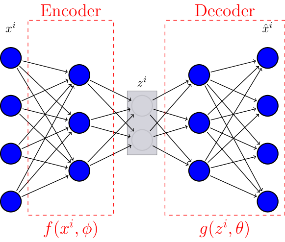
Figure 1: Auto-Encoder (AE) model.

III Background

In this section, we present the background of Auto-Encoder which is the basis of our proposed model.

Auto-Encoder (AE) is a popular representation learning paradigm that maps inputs to its representation [31]. More specifically, the AE is a neural network that attempts to reconstruct its input at the output using an unsupervised learning technique. An AE has two parts, an encoder and a decoder. Assume that $\textbf{W}^{e}$, $\textbf{b}^{e}$, $\textbf{W}^{d}$, and $\textbf{b}^{d}$ are the weight matrix and biases of the encoder and decoder, respectively. Let ${\phi}$ = (${\textbf{W}^{e}}$, ${\textbf{b}^{e}}$) be the parameter sets of the encoder function ${f_{\phi}}$, while ${\theta}$ = (${\textbf{W}^{d}}$, ${\textbf{b}^{d}}$) denotes the parameter sets of the decoder function ${g_{\theta}}$. Assume that a dataset X = $\{\textbf{x}^{1},\textbf{x}^{2},..,\textbf{x}^{n}\}$ is used for training the AE model, we can define $\textbf{z}^{i}=f_{\phi}(\textbf{x}^{i})$ as the feature-vector or the latent representation from $\textbf{x}^{i}$. The decoder function $g_{\theta}(\textbf{z}^{i})$ attempts to map the feature vector back into the input vector, producing a reconstruction $\hat{\textbf{x}}^{i}=g_{\theta}(\textbf{z}^{i})$. The common forms of the encoder and decoder are affine transformations as follows:

$$f_{\phi}(\textbf{x}^{i})=a_{f}(\textbf{W}^{e}\textbf{x}^{i}+\textbf{b}^{e}),$$ (1)

$$g_{\theta}(\textbf{z}^{i})=a_{g}(\textbf{W}^{d}\textbf{z}^{i}+\textbf{b}^{d}),$$ (2)

where $a_{f}$ and $a_{g}$ are active functions of the encoder and decoder, respectively.

The popular reconstruction error or loss function of the AE is the Mean-Squared-Error (MSE) function [32]:

$$\ell_{\mbox{AE}}(\textbf{x},\phi,\theta)=\frac{1}{n}\sum_{i=1}^{n}\left(\textbf{x}^{i}-\hat{\textbf{x}}^{i}\right)^{2}\cdot$$ (3)

The latent representation of the encoder is also referred to as a bottleneck which is used as an input for the following models. A good latent representation means that the classifiers achieve higher accuracy compared to those using the original datasets.

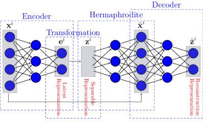
Figure 2: Twin Auto-Encoder (TAE) architecture.

IV Twin Auto-Encoder

This section presents a novel neural network architecture, namely Twin Auto-Encoder (TAE). TAE aims to learn a separable representation using the following two steps. First, the latent representation is transformed into a new separable representation using a transformation operator. Second, the twin structure is used to reconstruct the separable representation at the output. The detailed components of TAE are presented below.

IV-A Architecture of TAE

The TAE has three subnetworks, i.e., an encoder, a hermaphrodite, and a decoder, as illustrated in Fig. 2. The encoder maps an input sample $\textbf{x}^{i}$ into a latent vector $\textbf{e}^{i}$. After that, the latent vector $\textbf{e}^{i}$ is transformed into the separable representation $\textbf{z}^{i}$ using a transformation vector $\vec{\textbf{v}}$, as follows:

$$\textbf{z}^{i}=\textbf{e}^{i}+\vec{\textbf{v}},$$ (4)

where $\vec{\textbf{v}}$ (presented in detailed in Subsection IV-B) is the vector to transform from $\textbf{e}^{i}$ to $\textbf{z}^{i}$. Empirically, we found that the latent vectors, i.e., $\textbf{e}^{i}$, of different classes are often overlapped (see Subsection VII-A for the details). Thus, TAE aims to transform $\textbf{e}^{i}$ to $\textbf{z}^{i}$ to make $\textbf{z}^{i}$ more separable than $\textbf{e}^{i}$. The details of the transformation from $\textbf{e}^{i}$ to $\textbf{z}^{i}$ will be presented in Subsection IV-B.

The hermaphrodite connects the encoder and decoder thus it plays both decoding and encoding roles. On the decoding role, it reconstructs the input $\textbf{x}^{i}$ at $\hat{\textbf{x}}^{i}$ using the separable vector $\textbf{z}^{i}$. On the encoding role, the hermaphrodite maps the separable vector $\textbf{z}^{i}$ into a new space $\hat{\textbf{x}}^{i}$.

The third subnetwork in TAE is the decoder. The decoder attempts to reconstruct the separable representation i.e., $\textbf{z}^{i}$ at the output, i.e., $\hat{\textbf{x}}^{i}$. The output of TAE, i.e., $\hat{\textbf{x}}^{i}$, is called the reconstruction representation in the sense that it is reconstructed from the separable representation $\textbf{z}^{i}$. The reconstruction representation will be used as the final representation of TAE for the next detection models. During the inference or the testing time, the new data sample is input directly to the decoder to generate the reconstruction representation $\hat{\textbf{x}}^{i}$ and $\hat{\textbf{x}}^{i}$ is used for detecting cyberattacks .

Since $\textbf{z}^{i}$ is more distinguishable than $\textbf{e}^{i}$ (using the transformation operator in Subsection IV-B) and $\hat{\textbf{x}}^{i}$ is reconstructed from $\textbf{z}^{i}$, the reconstruction representation $\hat{\textbf{x}}^{i}$ can be more distinguishable than the latent representation $\textbf{e}^{i}$. Subsequently, this model, i.e., TAE is expected to facilitate the performance of the downstream attack detection approaches.

IV-B Transformation Operator

Input:

Dataset $\textbf{X}={\{\textbf{x}^{i,c}\}_{i=1}^{n}}$ where ${x}^{i,c}$ is $i^{th}$ samples in class $c$, $C$ is the set of all classes, $n_{c}$ is the number of samples in class $c\in C$, $|C|$ is the number of classes.

Output: $\bm{\mu}^{c}$, $\bm{\hat{\mu}}^{c}$, $\textbf{z}^{i,c}$

Step 1: Apply PCA to reduce the dimension of input data.

$\textbf{x}_{r}\leftarrow PCA(X)$

Step 2: Calculate mean $\bm{\mu}^{c}$ and center mean $\bm{\overline{\mu}}^{c}$.

foreach $c$ in $C$ do

       $\bm{\mu}^{c}\leftarrow\frac{1}{n_{c}}\sum_{i=1}^{n^{c}}(\textbf{x}^{i,c}_{r})$

end foreach

$\bm{\overline{\mu}}\leftarrow\frac{1}{|C|}\sum_{c=1}^{|C|}(\bm{\mu}^{c})$

Step 3: Calculate the transformed mean $\bm{\hat{\mu}}^{c}$ of $\bm{\mu}^{c}$ for each class $c$.

$\bm{\hat{\mu}}^{c}\leftarrow S^{c}\times{\textbf{t}}^{c}$

Step 4: Transform $\textbf{e}^{i,c}$ to a new representation $\textbf{z}^{i,c}$.

foreach $\textbf{x}^{i,c}$ in X do

       $\textbf{z}^{i,c}\leftarrow\textbf{e}^{i,c}+\vec{\textbf{V}}(\bm{\mu}^{c},\bm{\hat{\mu}}^{c})$

end foreach

Algorithm 1 Transforming the latent representation to separable representation

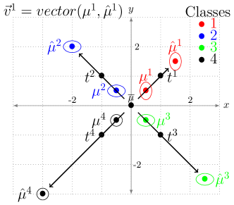
Figure 3: Transformation operator in TAE.

TABLE I: Calculating in TAE’s transformation operator.

Step 2
$\bm{\mu}^{i}$	$\bm{\mu}^{1}$	$\bm{\mu}^{2}$	$\bm{\mu}^{3}$	$\bm{\mu}^{4}$
$\bm{\mu}^{i}_{1}$	0.5	-0.5	0.5	-0.5
$\bm{\mu}^{i}_{2}$	0.5	0.5	-0.5	-0.5
$\bm{\overline{\mu}}=[0,0]$
Step 3
$\textbf{t}^{i}$	$\textbf{t}^{1}$	$\textbf{t}^{2}$	$\textbf{t}^{3}$	$\textbf{t}^{4}$
$\textbf{t}^{i}_{1}$	1	-1	1	-1
$\textbf{t}^{i}_{2}$	1	1	-1	-1
$S^{c}$	1.5	2	2.5	3
$\bm{\hat{\mu}}^{i}=S^{c}\times\textbf{t}^{i}$	$\bm{\hat{\mu}}^{1}$	$\bm{\hat{\mu}}^{2}$	$\bm{\hat{\mu}}^{3}$	$\bm{\hat{\mu}}^{4}$
$\bm{\hat{\mu}}^{i}_{1}$	1.5	-2	2.5	-3
$\bm{\hat{\mu}}^{i}_{2}$	1.5	2	-2.5	-3
Step 4
$\vec{\textbf{v}}^{i}=\bm{\hat{\mu}}^{i}-\bm{\mu}^{i}$	$\textbf{v}^{1}$	$\textbf{v}^{2}$	$\textbf{v}^{3}$	$\textbf{v}^{4}$
$\textbf{v}^{i}_{1}$	1	-1.5	2	-2.5
$\textbf{v}^{i}_{2}$	1	1.5	-2	-2.5

The important component in TAE is the operator to transform the latent representation $\textbf{e}^{i}$ into the separable presentation $\textbf{z}^{i}$. There are several potential approaches to design this operator. One possible solution is to transform the latent representation of different classes into different corners of a hyper-cube. Another is to uniformly spread the representation of different classes in a super sphere. In this paper, we propose a simple yet effective approach to transform the latent representation into a separable representation based on data samples in each class.

Our approach is based on transforming the center/mean of data samples in each class to different directions. Specifically, we calculate the mean of the whole dataset (called $\bm{\overline{\mu}}$) and then transform the mean of each class to different directions from the $\bm{\overline{\mu}}$. Algorithm 1 presents the four steps to transform $\textbf{e}^{i}$ to $\textbf{z}^{i}$ in detail.

• The first step is to reduce the dimension of the original dataset $X$ to the dimension of the latent vector $\textbf{e}^{i}$ using use the PCA [33] method.

• The second step calculates a mean $\bm{\mu}^{c}$ of each class $c$ and the mean $\bm{\overline{\mu}}$ of the means of all classes.

• The third step calculates the new mean, i.e., the mean after transforming, $\bm{\hat{\mu}}^{c}$, of each class $c$ by Equation $\bm{\hat{\mu}}^{c}=S^{c}\times\textbf{t}^{c}$, where $\textbf{t}^{c}$ is the direction to transform from $\bm{\mu}^{c}$ to $\bm{\hat{\mu}}^{c}$, and $S^{c}$ is the scale of the transformation .

• The fourth step is to transform the latent vector $\textbf{e}^{i,c}$ of class $c$ to a new vector $\textbf{z}^{i,c}$ following the direction of vector $\vec{\textbf{v}}^{c}$ that connects the old mean $\bm{\mu}^{c}$ to the new mean $\bm{\hat{\mu}}^{c}$, i.e., $\vec{\textbf{v}}^{c}=\vec{\textbf{V}}(\bm{\mu}^{c},\bm{\hat{\mu}}^{c})$.

Fig. 3 illustrates an example of transforming data samples in the two-dimensional latent space. A simulation training dataset has four classes with the means in the latent space $\bm{\mu}^{1}$, $\bm{\mu}^{2}$, $\bm{\mu}^{3}$, and $\bm{\mu}^{4}$, respectively. The center mean $\bm{\overline{\mu}}$ of the whole data samples in the training dataset is calculated in Step 2 in Table I. In Step 3, $\textbf{t}^{1}$, $\textbf{t}^{2}$, $\textbf{t}^{3}$ and $\textbf{t}^{4}$ are determined and used to calculate $\bm{\hat{\mu}}^{1}$, $\bm{\hat{\mu}}^{2}$, $\bm{\hat{\mu}}^{3}$ and $\bm{\hat{\mu}}^{4}$, respectively. Finally, vectors, i.e., $\textbf{v}^{1}$, $\textbf{v}^{2}$, $\textbf{v}^{3}$, and $\textbf{v}^{4}$, are calculated in Step 4, and they are used to transform latent vectors into the separable vectors. It can be seen from Fig. 3 that, although $\bm{\mu}^{1}$, $\bm{\mu}^{2}$, $\bm{\mu}^{3}$, and $\bm{\mu}^{4}$ are relatively close together, the new means, i.e., $\bm{\hat{\mu}}^{1}$, $\bm{\hat{\mu}}^{2}$, $\bm{\hat{\mu}}^{3}$ and $\bm{\hat{\mu}}^{4}$ are transformed to more separated positions.

IV-C Loss Function of TAE

TAE is trained in the supervised mode using the label information in the datasets. The loss function of TAE for a dataset $X={\{\textbf{x}^{i}\}_{i=1}^{n}}$ with the labels $Y={\{{\textbf{y}}^{i}\}_{i=1}^{n}}$, includes three terms as follows:

$$\ell_{\mbox{TAE}}=\frac{1}{n}\sum_{i=1}^{n}\big{[}(\textbf{x}^{i}-\hat{\textbf{x}}^{i})^{2}+(\textbf{z}^{i}-\hat{\textbf{z}}^{i})^{2}+(\textbf{e}^{i}-\bm{{\mu}}^{c})^{2}],$$ (5)

where $\textbf{x}^{i}$ is the $i^{th}$ data sample and $\hat{\textbf{x}}$ is the representation at the output layer of the hermaphrodite. $\textbf{e}^{i}$ is the representation of $\textbf{x}^{i}$ in the latent space, $\textbf{z}^{i}$ is the separable representation transformed from $\textbf{e}^{i}$ and $\hat{\textbf{z}}^{i}$ is the reconstruction representation, i.e. the output of TAE. Finally, $\bm{{\mu}}^{c}$ the mean of data samples in class $c$ calculated in Step 2 of Algorithm 1).

The first term in Equation (5) is the reconstruction error between $\textbf{x}^{i}$ and $\hat{\textbf{x}}$. The next term is also reconstruction errors between $\textbf{z}^{i}$ and $\hat{\textbf{z}}^{i}$. The third term aims to shrink the latent vector $\textbf{e}^{i}$ of TAE into its mean $\bm{\mu}^{c}$ of each class. This term prevents the latent representation $\textbf{z}^{i}$ of different classes from being overlapped.

IV-D Training TAE Model

We use the ADAM optimization algorithm [34] and the mini-batch method [35] to train the TAE model. Moreover, both $\textbf{x}^{i}$ and $\hat{\textbf{x}}^{i}$ are used as the input to the decoder in the training process. This is to facilitate TAE reconstructing the separable representation well during the inference .

V Experimental settings

This section presents the settings in the experiments. We first discuss the performance metrics used to measure the performance of the tested models. The datasets and the hyper-parameters settings are presented after that.

TABLE II: Datasets information.

Datasets	ID	No. Train	No. Valid	No. Test	No. Classes	No. Features
DanG [10]	IoT1	179434	76901	109863	6	115
EcoG [10]	IoT2	158631	67986	97126	6	115
PhiG [10]	IoT3	239099	102472	146392	6	115
737G [10]	IoT4	192200	82372	117678	6	115
838G [10]	IoT5	199698	85586	122270	6	115
EcoMG [10]	IoT6	409574	175533	250769	11	115
838MG [10]	IoT7	410071	175746	251074	11	115
NSLKDD [12]	NSL	88181	37792	22544	5	41
UNSW-NB15 [16]	UNSW	57632	24700	175341	10	42
IoT Malware 1 [17]	Mal1	57544	14387	8888	2	32
IoT Malware 2 [17]	Mal2	6498	1625	2603	2	32
IoT Malware 3 [17]	Mal3	10183	2546	53624	2	32
Cloud IDS [18]	Cloud	1239381	517915	887113	7	24

TABLE III: Neural network settings for MAE and MVAE.

Datasets	Input	$h1$	$z$	$h2$	$\hat{x}$
IoTs	115	50	10	50	115
IDSs	41, 42	30	6	30	41, 42
Malware	32	20	6	20	32
Cloud	24	15	5	15	24

TABLE IV: Neural network settings for TAE.

Datasets	Input	$h1$	$z$	$h2$	$\hat{x}$	$h3$	$\hat{z}$
IoTs	115	50	10	50	115	50	10
IDSs	41, 42	30	6	30	41, 42	30	6
Malware	32	20	6	20	32	20	6
Cloud	24	15	5	15	24	15	5

TABLE V: Grid search settings for machine learning models.

LR $C$={0.1, 0.5, 1.0, 5.0, 10.0} SVM LinearSVC: $C$={0.1, 0.2, 0.5, 1.0, 5.0, 10.0} SVC: $decision\_function\_shape={ovo}$ DT $max\_depth$={5, 10, 20, 50, 100} RF $n\_estimators$={5, 10, 20, 50, 100, 150} Xgb $min\_child\_weight$={5,10}, $gamma$={0.5, 1.5}, $subsample$={1.0, 0.9}

TABLE VI: Grid search settings for TAE.

$S$ $S$={0.0001, 0.01, 0.1, 0.2, 0.5, 1.0}; $S$={5, 10, 20, 40, 80} $D_{z}$ $D_{z}$={1, 2, 5, 10, 15, 20, 30, 40}; Active function Relu, Tanh

V-A Performance Metrics

We use four popular metrics, i.e., ${Accuracy}$, $F\mbox{-}score$ [36], Miss Detection Rate (MDR), and False Alarm Rate (FAR), to evaluate the performance in the experiments [23].

The accuracy metric is calculated as follows:

$${Accuracy}=\frac{\emph{TP}+\emph{TN}}{\emph{TP}+\emph{TN}+\emph{FP}+\emph{FN}}\cdot$$ (6)

where TP is True Positive, FP is False Positive, TN is True Negative and FN is False Negative.

The $F\emph{-}score$ is the harmonic mean of the precision and the recall, which is an effective metric for imbalanced datasets:

$${F\emph{-}score}=2\times\frac{{Precision}\times{Recall}}{{Precision}+{Recall}}\cdot$$ (7)

where Precision is the ratio of the number of correct detection to the number of incorrect detection and Recall is the ratio of the number of correct detection to the number of false detection.

The Miss Detection Rate (MDR) [15] is a ratio of the not detected positive samples to a total of real positive samples:

$$\emph{MDR}=\frac{\emph{FN}}{\emph{FN}+\emph{TP}}\cdot$$ (8)

The False Alarm Rate (FAR) is the ratio of the number of false alarms of negative samples to the total number of real negative samples:

$$\emph{FAR}=\frac{\emph{FP}}{\emph{FP}+\emph{TN}}\cdot$$ (9)

The values of both scores MDR and FAR are equal $0$ when the number of miss detections of positive samples and the number of false alarms of negative samples are equal $0$.

V-B Datasets

We use a wide range of datasets in cybersecurity to evaluate the effectiveness of TAE. The tested datasets include the IoT botnet attacks datasets, the network IDS datasets, the cloud DDoS attack dataset, and the malware datasets. The number of training, validation, and testing samples of each dataset are presented in Table II. The number of classes, the number of features, and the shorthand (ID) of each dataset are also shown in this Table.

The IoT botnet datasets [10] include seven different datasets. These seven datasets are Danmini Doorbell (Dan), Ecobee Thermostat (Eco), Philips B120N10 Baby Monitor (Phi), Provision PT 737E Security Camera (737), and Provision PT 838 Security Camera (838) [10]. The datasets consist of two types of attacks, i.e., Gafgyt and Mirai attacks. We perform two scenarios on these multiclass datasets. The first scenario includes the normal traffic and five types of the Gafgyt attacks that form the six classes classification problem, whilst the second scenario consists of the normal traffic, five types of the Mirai attacks, and five types of the Gafgyt attacks forming the 11 classes problem. The dataset name is shorthanded by the name of the dataset and the type of attacks. For instance, EcoG means the Ecobee dataset and the Gafgyt attack, while EcoMG is the Ecobee dataset with both Mirai and Gafgyt attacks.

The IDS datasets consist of the NSLKDD (NSL)[12] and the UNSW-NB15 (UNSW) [16] dataset. The NSL dataset was proposed to surpass the inherent issues of the KDD Cup 99 dataset. The data in the NSL includes the benign traffic and four types of attacks, i.e., DoS, R2L, Probe, and U2L. Among the four types of attacks, R2L and U2L are two sophisticated and rare attacks that are very challenging to be detected by machine learning algorithms [37]. The UNSW dataset has benign traffic and nine types of attacks. This dataset has 42 features that are aggregated from the traffic features. Both NSL and UNSW datasets are imbalanced datasets. This is because the number of samples of R2L and U2R attacks in NSL and Worms, Backdoor, and Shellcode attacks in UNSW are significantly lower than those of others.

The malware datasets are generated by Avast AIC laboratory to collect 20 malware families on IoT systems [17]. There are three binary malware datasets, e.g., Mal1, Mal2, and Mal3. Each data sample has 32 features. The training sets include benign samples and typical malware families, e.g., DDoS and Part-of-Horizontal-Port-Scan while the testing sets consist of benign samples and more sophisticated malware classes, e.g., C&C-attack, Okiru, C&C-heartbeat, C&C-Mirai, and C&C-PortScan. This means that some malware in the testing sets is not available in the training set. Thus, it is difficult for ML models to detect this unknown malware in the testing set.

The cloud IDS datasets are DDoS attacks on the cloud environment. They are published by Kumar et al. [18] by stimulating the cloud environment and using an open-source platform to launch 15 normal VMs, 1 target VM, and 3 malicious VMs. The extracted datasets contain 24 time-based traffic flow features. The cloud IDS datasets are also divided into training and testing sets with a rate of 70:30.

V-C Hyper-parameters Setting

This subsection presents the hyper-parameter settings for tested methods in the experiments. The tested methods include MVAE and MAE [15], CSAEC [19] [38]. In addition, we also compare TAE with popular machine learning models including Multi-Layer Perceptron (MLP) [39], Support Vector Machine (SVM), Decision Tree (DT), Random Forest (RF), One-dimensional Convolutional Neural Network (1D-CNN), Multi-Layer Perceptron (MLP) and the state-of-the-art Xgboost (Xgb) [20].

The experiments are implemented using two frameworks: TensorFlow and Scikit-learn [40]. All datasets are normalized using Min-Max normalization [41]. We also use grid search to tune the hyper-parameters for each machine learning model, as shown in Table V. The other parameters for machine learning models are the default values in Scikit-learn. The configuration for 1D-CNN is taken from [42] where 16 convolution filters, 3 kernel sizes, and 2 time steps in the convolution layer are used. We use the leaky Relu function in the convolution layers. The numbers of features inputting to 1D-CNN (after padding) of IoT, NSL, UNSW, Cloud, and Malware datasets are 116, 44, 44, 24, and 32, respectively. For the representation learning methods, the final representation is extracted and used as the input to the Decision Tree (DT) model, and the performance of DT is reported in the experiments .

For all neural network models, i.e., MAE, MVAE, TAE, only one hidden layer with Relu activation is used in their subnetworks (the encoder, hermaphrodite, and decoder). The optimization algorithm to train these models is ADAM [34]. The learning rate $\alpha$ is set at $10^{-4}$, the number of epochs is 5000 and the batch size is set at 100. We also use the validation set to early stop during the training process. 30% of the training set is used for the validation set, whilst the remaining 70% is used for training the models. If the difference value of the loss function between 10 epochs is lower than a $threshold=1$, we stop the training process. The weights and biases of the neural networks are initialized using the Glorot method [43]. The numbers of neurons in the layers of MAE and MVAE are given in Table III, and the parameters for TAE are given in Table IV. In these tables, $d_{x}$ is the size of the original data and $d_{z}$ is the size of the latent representation. For MAE and MVAE, $|h_{1}|$, $|h_{2}|$ are the numbers of neurons in the layer of the encoder and decoder, respectively. For TAE, $|h_{1}|$, $|h_{2}|$, $|h_{3}|$ are the neurons of the encoder, hermaphrodite, and decoder. For each dataset, the number of neurons in the bottleneck layer is tuned by a list of $d_{z}$, $2\times d_{z}$, and $3\times d_{z}$. $d_{z}$ is configured by the rule $d_{z}\approx\sqrt{d_{x}}$ in [44, 15, 45], where $d_{x}$ is the dimension of the input data.

MAE and MVAE models are only investigated on binary datasets in [15]. In this paper, we extend the approaches in  [15] for multi-classes problems by setting the value of $\mu^{c}_{j}$ from $2$ to $n+2$, where $n$ is the number of classes. For CSAE, the same architecture in [38] is built using 1D convolution. After training CSAE in an unsupervised learning manner, we add a softmax layer to the encoder of CSAE, and the CSAE is trained in a supervised learning method. After that, the softmax layer is removed and this configuration is referred to as CSAEC [30]. Finally, for the TAE model, we also tune two hyper-parameters, i.e. the scale of the transformation operator $S$ in Algorithm 1 and the dimensionality of the latent space $D_{z}$, as shown in Table VI.

TABLE VII: Performance of TAE compared to SCAEC, MVAE, and MAE.

		IoTs							IDSs		Cloud	Malware
Measures	Methods	IoT1	IoT2	IoT3	IoT4	IoT5	IoT6	IoT7	NSL	UNSW	Cloud	Mal1	Mal2	Mal3
	SCAEC	0.923	0.914	0.941	0.933	0.928	0.882	0.929	0.843	0.734	0.980	0.512	0.889	0.920
	MVAE	0.688	0.608	0.751	0.654	0.713	0.536	0.747	0.829	0.681	0.867	0.514	0.687	0.929
	MAE	0.921	0.913	0.943	0.922	0.931	0.757	0.933	0.841	0.662	0.952	0.414	0.917	0.921
Accuracy	TAE	0.931	0.933	0.985	0.949	0.993	0.959	0.975	0.873	0.747	0.987	0.517	0.914	0.955
	SCAEC	0.895	0.887	0.919	0.915	0.899	0.886	0.923	0.798	0.692	0.980	0.432	0.887	0.928
	MVAE	0.642	0.528	0.666	0.536	0.702	0.617	0.713	0.779	0.623	0.819	0.435	0.683	0.935
	MAE	0.893	0.885	0.922	0.893	0.908	0.750	0.934	0.793	0.637	0.951	0.248	0.917	0.929
F-score	TAE	0.916	0.922	0.985	0.944	0.993	0.949	0.970	0.844	0.695	0.987	0.439	0.912	0.958
	SCAEC	0.015	0.017	0.008	0.012	0.012	0.015	0.006	0.150	0.079	0.034	0.339	0.153	0.064
	MVAE	0.112	0.158	0.060	0.111	0.083	0.056	0.032	0.147	0.094	0.534	0.337	0.363	0.101
	MAE	0.015	0.017	0.008	0.015	0.013	0.039	0.008	0.146	0.090	0.109	0.407	0.108	0.039
FAR	TAE	0.013	0.013	0.002	0.009	0.001	0.003	0.002	0.117	0.073	0.027	0.335	0.124	0.056
	SCAEC	0.077	0.086	0.059	0.067	0.072	0.118	0.071	0.157	0.266	0.020	0.488	0.111	0.080
	MVAE	0.312	0.392	0.249	0.346	0.287	0.367	0.253	0.171	0.319	0.133	0.486	0.313	0.071
	MAE	0.079	0.087	0.057	0.078	0.075	0.243	0.084	0.159	0.338	0.048	0.586	0.083	0.079
MDR	TAE	0.069	0.067	0.015	0.051	0.007	0.041	0.025	0.127	0.263	0.013	0.483	0.086	0.045

TABLE VIII: Performance of TAE compared to popular machine learning models.

		IoTs							IDSs		Cloud	Malware
Measures	Methods	IoT1	IoT2	IoT3	IoT4	IoT5	IoT6	IoT7	NSL	UNSW	Cloud	Mal1	Mal2	Mal3
	Xgb	0.923	0.910	0.941	0.921	0.928	0.941	0.959	0.872	0.762	0.985	0.419	0.607	0.921
	SVM	0.670	0.612	0.751	0.655	0.708	0.837	0.856	0.844	0.672	0.890	0.409	0.720	0.939
	DT	0.672	0.654	0.753	0.656	0.740	0.844	0.867	0.866	0.743	0.977	0.414	0.544	0.918
	RF	0.672	0.613	0.752	0.656	0.709	0.850	0.858	0.871	0.757	0.983	0.416	0.777	0.921
	1D-CNN	0.635	0.613	0.752	0.654	0.709	0.820	0.846	0.839	0.703	0.980	0.474	0.674	0.911
	MLP	0.706	0.739	0.810	0.733	0.780	0.724	0.856	0.861	0.722	0.926	0.414	0.719	0.954
Accuracy	TAE	0.931	0.933	0.985	0.949	0.993	0.959	0.975	0.873	0.747	0.987	0.517	0.914	0.955
	Xgb	0.894	0.879	0.918	0.891	0.900	0.929	0.945	0.830	0.733	0.985	0.259	0.608	0.929
	SVM	0.553	0.475	0.662	0.535	0.603	0.784	0.805	0.794	0.606	0.842	0.238	0.670	0.944
	DT	0.557	0.547	0.665	0.536	0.658	0.799	0.824	0.828	0.720	0.977	0.250	0.545	0.926
	RF	0.557	0.477	0.664	0.536	0.604	0.797	0.807	0.827	0.727	0.982	0.252	0.751	0.929
	1D-CNN	0.515	0.477	0.663	0.534	0.605	0.768	0.796	0.788	0.646	0.979	0.366	0.635	0.920
	MLP	0.605	0.651	0.744	0.645	0.703	0.635	0.815	0.822	0.671	0.913	0.248	0.670	0.956
F-score	TAE	0.916	0.922	0.985	0.944	0.993	0.949	0.970	0.844	0.695	0.987	0.439	0.912	0.958
	Xgb	0.015	0.018	0.008	0.015	0.012	0.005	0.003	0.120	0.064	0.035	0.404	0.342	0.050
	SVM	0.117	0.159	0.061	0.111	0.088	0.019	0.018	0.148	0.120	0.528	0.410	0.427	0.023
	DT	0.117	0.151	0.060	0.111	0.083	0.019	0.017	0.118	0.069	0.039	0.407	0.491	0.039
	RF	0.117	0.159	0.060	0.111	0.088	0.019	0.018	0.124	0.068	0.043	0.406	0.340	0.046
	1D-CNN	0.117	0.159	0.059	0.111	0.088	0.022	0.020	0.144	0.101	0.037	0.365	0.454	0.073
	MLP	0.140	0.104	0.053	0.096	0.076	0.048	0.021	0.133	0.093	0.339	0.407	0.427	0.089
FAR	TAE	0.013	0.013	0.002	0.009	0.001	0.003	0.002	0.117	0.073	0.027	0.335	0.124	0.056
	Xgb	0.076	0.094	0.059	0.079	0.072	0.046	0.041	0.128	0.238	0.015	0.581	0.393	0.079
	SVM	0.328	0.388	0.249	0.345	0.292	0.163	0.144	0.156	0.328	0.110	0.591	0.280	0.061
	DT	0.328	0.346	0.247	0.344	0.260	0.156	0.133	0.134	0.257	0.023	0.586	0.456	0.082
	RF	0.328	0.387	0.247	0.344	0.291	0.150	0.142	0.129	0.243	0.017	0.584	0.223	0.079
	1D-CNN	0.328	0.388	0.275	0.345	0.292	0.201	0.150	0.161	0.297	0.020	0.526	0.326	0.089
	MLP	0.294	0.261	0.190	0.267	0.220	0.276	0.144	0.139	0.278	0.074	0.586	0.281	0.046
MDR	TAE	0.069	0.067	0.015	0.051	0.007	0.041	0.025	0.127	0.263	0.013	0.483	0.086	0.045

VI PERFORMANCE ANALYSIS

This section evaluates the performance of TAE and compares it with the state-of-the-art Auto-Encoders and deep learning models for cyberattack detection. Moreover, popular machine learning models are also compared with the performance of TAE. The main experimental results are shown in Table VII and Table VIII.

VI-A Accuracy of Detection Models

Table VII presents the performance of TAE compared to the other RL methods on the tested datasets. In this table, the best results on each dataset for each performance metric are printed in boldface. Apparently, TAE achieves the best accuracy in all configurations except on the Mal2 dataset . For example on the IoT2 dataset, the accuracy of TAE is 0.933 while the accuracy of SCAEC, MVAE, and MAE are only 0.914, 0.608, and 0.913, respectively. The accuracy of TAE on the IDS, Cloud, and Malware datasets is also very convincing. For instance, the accuracy of TAE on Mal3 is 0.955 compared to that of SCAEC MVAE and MAE are 0.920, 0.925, and 0.921, respectively. Considering $F\emph{-}score$ metric, the table shows that the $F\emph{-}score$ of TAE is always higher than that of the others. On the EcoG dataset, the $F\emph{-}score$ of TAE is 0.922 compared to 0.887, 0.528, and 0.885 of SCAEC, MVAE, and MAE, respectively. Amongst the four tested methods, the table shows that MVAE achieves the worst performance. The reason is that the latent representation of MVAE is nondeterministic due to the random sampling process to generate the latent representation. Thus, the latent representation of MVAE is not as stable as that of the others. Similar results are also observed with two metrics FAR and MDR, i.e., the values of TAE is smallest on all tested problems except Mal2.

Table VIII presents the performance of TAE compared to six popular machine learning models, i.e., SVM, DT, RF, 1D-CNN, MLP, and Xgb, on the tested datasets. There are two interesting results in this table. First, the performance of TAE is often much better than the others except the Xgb model. For example, on the IoT1 dataset, the accuracy of TAE is 0.931 while the accuracy of SVM, DT, RF, 1D-CNN, and MLP are only 0.670, 0.672, 0.672, 0.635, and 0.706, respectively. This result shows that the original representation of data of the tested problems is difficult for conventional machine learning methods. However, by transforming from the original representation to the separable representation and then reconstructing the separable representation by the reconstruction representation of TAE, the representation of data is much easier for the machine learning models. Second, only the model that performs closely to TAE is Xgb. This is not surprising since Xgb is one of the best machine learning models introduced recently. However, the table also shows that the performance of TAE is still better than that of the state-of-the-art model, i.e., Xgb. Moreover, the complexity of TAE is much less than that of Xbg (shown in the next section). Thus, TAE is more applicable in cyberattack detection than Xgb.

Overall, the above results show the superior performance of the proposed model, i.e., TAE over the other representation learning and machine learning algorithms on a wide range of cybersecurity problems. TAE is trained in the supervised mode, and its performance is usually better than that of the state-of-the-art representation models, i.e., MAE, and SCAEC. TAE also shows superior performance over well-known machine learning models using the original datasets, i.e., SVM, DT, RF, 1D-CNN, and MLP. In addition, the results of TAE are almost higher than the advanced ensemble learning method (Xgb).

TABLE IX: Confusion matrix of TAE, MAE, and Xgb on the NSL dataset.

Metthods	Classes	Normal	DoS	U2R	R2L	Probe
	Normal	9475	56	5	23	152
	DoS	150	5557	0	0	34
	U2R	23	2	10	0	2
	R2L	1689	7	22	475	6
TAE	Probe	223	2	0	0	881
	Normal	9441	93	4	14	159
	DoS	301	5333	1	11	95
	U2R	25	7	1	2	2
	R2L	1986	109	3	79	22
MAE	Probe	253	7	1	0	845
	Normal	9428	81	1	0	201
	DoS	12	5716	0	0	13
	U2R	31	0	4	2	0
	R2L	2037	0	1	135	26
Xgb	Probe	1	0	0	0	1105

TABLE X: Confusion matrix of TAE, MAE, and Xgb on the Cloud dataset.

Methods	Classes	$l_{1}$	$l_{2}$	$l_{3}$	$l_{4}$	$l_{5}$	$l_{6}$	$l_{7}$
	normal traffic ($l_{1}$)	1151	0	0	5	0	0	0
	Dns-flood ($l_{2}$)	0	6	0	0	0	0	5
	Ping-of-death ($l_{3}$)	0	0	18	0	0	0	0
	Slowloris ($l_{4}$)	7	0	0	138	0	0	0
	Tcp-land-attack ($l_{5}$)	0	0	0	0	11	0	0
	TCP-syn-flood ($l_{6}$)	0	0	0	0	0	19	0
TAE	Udp-flood ($l_{7}$)	0	1	0	0	0	0	13
	normal traffic ($l_{1}$)	1144	0	0	12	0	0	0
	Dns-flood ($l_{2}$)	0	5	0	0	1	1	4
	Ping-of-death ($l_{3}$)	0	1	12	0	2	3	0
	Slowloris ($l_{4}$)	28	0	0	117	0	0	0
	Tcp-land-attack ($l_{5}$)	0	0	0	0	8	2	1
	TCP-syn-flood ($l_{6}$)	0	1	1	0	3	13	1
MAE	Udp-flood ($l_{7}$)	0	3	0	0	0	2	9
	normal traffic ($l_{1}$)	1153	0	0	3	0	0	0
	Dns-flood ($l_{2}$)	0	6	0	0	0	0	5
	Ping-of-death ($l_{3}$)	0	0	18	0	0	0	0
	Slowloris ($l_{4}$)	9	0	0	136	0	0	0
	Tcp-land-attack ($l_{5}$)	0	0	0	0	11	0	0
	Tcp-syn-flood ($l_{6}$)	0	0	0	0	0	19	0
Xgb	Udp-flood ($l_{7}$)	0	3	0	0	0	0	11

TABLE XI: Confusion matrix of TAE, MAE, and Xgb on the Mal3 dataset.

Methods	Classes	Mal3
		Normal	Attacks
TAE	Normal	5586	344
	Attacks	2059	45635
MAE	Normal	5725	205
	Attacks	4013	43681
Xgb	Normal	5677	253
	Attacks	3986	43708

VI-B Detecting Sophisticated Attacks

This section analyses the ability of TAE to detect sophisticated, challenging, and unknown attacks. Specifically, the capability of TAE to detect the R2L and U2R attacks in the NSL dataset, the Ping-of-dead, Slowloris, and Tcp-land attacks in the Cloud dataset, and various unknown attacks in the Mal3 dataset are investigated. We also compare the accuracy of TAE with one state-of-the-art RL method, i.e., MAE, and one state-of-the-art machine learning method, i.e., Xgb.

R2L and U2R are two sophisticated attacks in the NSL dataset that are difficult for conventional machine learning models [46]. U2R attacks involve exploiting vulnerabilities in the system to gain superuser or root privileges. These attacks often produce subtle and limited changes in system behavior, which can be difficult to distinguish from normal system activities. R2L attacks typically occur when an attacker tries to gain unauthorized access to a remote system, such as through exploiting vulnerabilities or using brute force attacks on login credentials. These attacks often involve relatively low network traffic, making them less conspicuous and very hard to detect.

The confusion metric of the tested methods on the NSL dataset is shown in Table IX. It can be observed from Table IX that while MAE and Xgb are difficult to detect these two attacks, the ability to detect them of TAE is much better. Specifically, TAE is able to detect 10 out of 37 U2R attack samples while these values for MAE and Xgb are only 1 and 4. For R2L attacks, TAE correctly detects 475 out of 2199 while MAE and Xgb are able to detect only 79 and 135, respectively. For the false alarm, the table shows that the false alarm of TAE is often much smaller than MAE and it is only slightly higher than that of Xgb. Overall, the result in this table shows that the DT classifier trained on the representation of TAE is able to detect rare and sophisticated attacks much better than MAE and Xgb, although, the false alarm of TAE is slightly higher than Xgb.

Ping-of-dead, Slowloris, and Tcp-land attacks are three shuttle attacks on the Cloud dataset [18]. Ping-of-death attacks exploit vulnerabilities in network protocols like ICMP (Internet Control Message Protocol). However, ICMP is a fundamental part of the Internet’s infrastructure, and it is used for many legitimate services such as network diagnostics, troubleshooting, and connectivity checks. Thus, distinguishing between legitimate and malicious ICMP packets is a difficult task. TCP-land and Slowloris attacks typically involve sending a relatively small number of packets to the target, often just a few packets per second. This low attack volume can blend with other legitimate network traffic, making it harder to spot anomalous behavior.

The confusion metric of the tested methods on the Cloud dataset is shown in Table X in which the results on the Ping-of-dead, Slowloris, and Tcp-land attacks are highlighted. It can be seen that the performance of TAE is considerably higher than the performance of MAE on these attacks. For example, on the Slowloris attack, TAE correctly identifies 138 out of 145 samples while MAE is only correct on 117 out of 145 samples. Similar results are also observed with the two other attacks, i.e., Ping-of-dead, Slowloris, and Tcp-land attacks. Comparing TAE and Xgb, the table shows that they are mostly equal except for the Slowloris attack where TAE is slightly better than Xgb. Moreover, TAE is less complex than Xgb as shown in the next section. Thus, it is more applicable than Xgb in the cybersecurity domain.

The last set of experiments in this subsection is to analyze the performance of TAE, MAE, and Xgb on Mal3 datasets. The training set of Mal3 contains the normal traffic and only one type of attack (DDoS attack) while its testing set contains many types of unknown attacks such as C&C-Heart-Beat-Attack, C&C-Heart-Beat-File-Download, C&C-Part-Of-A-Horizontal-Port-Scan, Okiru, Part-Of-A-Horizontal-Port-Scan-Attack [17]. The confusion metrics of these methods on Mal3 are presented in Table XI.

It can be seen that TAE is capable of detecting attacks much better than both MAE and Xgb. Specifically, TAE correctly detected 45635 out of 47694 compared to the value of MAE and Xgb is only 43681 and 43708. Although the false positive of TAE is slightly higher than the value of MAE and Xgb (344 vs 205 and 253), the false positive rate of TAE is still relatively low (344/45635 = 0.75%). This result evidences the ability of TAE to identify unknown attacks in malware datasets.

VII TAE ANALYSIS

This section analyses TAE to understand its characteristics. We first analyze the simulation visualization and the representation quality. After that, the effectiveness of the separable representation and the latent representation is compared. Next, the influence of hyper-parameters on the performance of the TAE model is discussed. Finally, we visualize the loss function of TAE and analyze the complexity of the TAE model. Due to the limited space, each experiment is conducted on only a subset of all datasets.

TAE Train
	4a. Original data	4b. Latent vector($\textbf{e}^{i}$)	4c. Reconstruction vector ($y$)
TAE Test
	4d. Original data	4e. Latent vector($\textbf{e}^{i}$)	4f. Reconstruction vector ($y$)

Figure 4: Simulation of data representation on the IoT3 dataset.

VII-A Representation Visualization

This subsection analyses various representations of TAE by visualizing them in the 2D space. Fig. 4 presents the distribution of the different vectors (representation) of TAE on the IoT3 dataset. To facilitate the representation, the dimension of the latent vector is set at 2. Figs. 4a, 4b and 4c show simulation on the training data while Figs. 4d, 4e and 4f show the simulation on the testing data. Fig. 4a and Fig. 4d show original data reduced into two dimensions by PCA, respectively. The latent representation of TAE on the training/testing datasets is shown in Fig. 4b and Fig. 4e, respectively, while Fig. 4c and Fig. 4f are of reconstruction representation ($\textbf{y}^{i}$) on training/testing datasets.

It can be seen that the original data samples in the training/testing datasets (Fig. 4a and Fig. 4f) are overlapped. In the latent space, the data samples are still mixed. This shows that using the latent vector for the downstream tasks may not be effective. Conversely, most data samples in the reconstruction representation of TAE are well separated (Fig. 4e and Fig. 4h). For example, data samples from Benign and UDP in the original datasets are overlapped together on both training/testing datasets, while they are much more separated in both Fig. 4e and Fig. 4h. In addition, as observed in Fig. 4b and Fig. 4g, most of the data samples in the reconstruction representation are shrunk in a small region. This makes it easier to classify the data samples of different classes.

VII-B Representation Quality

TABLE XII: Representation quality the original data the reconstruction representation.

Data	Between-class		Within-class		Representation quality
	Orig	TAE	Orig	TAE	Orig	TAE
IoT1	1.1	2.9	1.6E-3	2.1E-3	7.0E+02	1.4E+03
IoT2	1.2	4.1	1.9E-3	704E-6	6.5E+02	5.8E+03
IoT3	1.1	3.8	2.1E-3	25E-6	5.5E+02	1.5E+05
IoT4	1.2	3.3	2.9E-3	1.4E-3	4.0E+02	2.4E+03
IoT5	1.2	3.7	4.0E-3	61E-6	2.9E+02	6.0E+04
IoT6	4.1	5.2	13.8E-3	1.6E-3	3.0E+02	3.4E+03
IoT7	3.2	6.0	9.8E-3	1.6E-3	3.3E+02	3.8E+03

To further explain the superior performance of the TAE, we follow the idea from [47] to evaluate the quality of the reconstruction representation in TAE. Specifically, we use two measures to quantify the representation quality, i.e., the average distance between means of classes, $d_{Bet}$, and the average distance between data samples with their mean $d_{Wit}$. Moreover, we also introduce a new harmonic measure called the representation-quality that is calculated as $representation\mbox{-}quality=\frac{d_{Bet}}{d_{Wit}}$. A good representation is the one that samples $\textbf{x}^{i,c}$ of class $c$ is closer to its mean $\mu^{c}$, whilst the distance between means of classes are as the largest. In other words, if the value of $representation\mbox{-}quality$ is greater, the better the representation is.

Table XII presents the representation quality of the original data (Orig) $\textbf{x}^{i}$ and the reconstruction representation $\hat{\textbf{z}}^{i}$ in TAE on the IoT datasets. It is clear that the value of $represenation\mbox{-}quality$ obtained by the reconstruction representation in TAE is much greater than that obtained by the original data. This provides more pieces of evidence to explain the better performance obtained by the reconstruction representation of TAE compared to the original data.

VII-C Reconstruction Representation vs Latent Representation

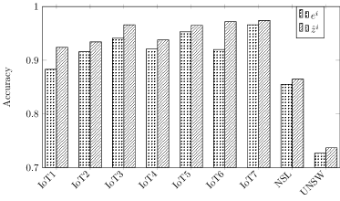
Figure 5: Performance of DT using the latent representation($\textbf{e}^{i}$) and the reconstruction representation (${\hat{\textbf{z}}}^{i}$).

To extensively investigate the effectiveness of the reconstruction representation over the latent representation, we conduct one more experiment to compare the accuracy of the detection model (Decision Tree) using the latent representation $\textbf{e}^{i}$ and the reconstruction representation $\hat{\textbf{z}}^{i}$. The results are shown in Fig. 5. Apparently, the accuracy obtained by $\textbf{y}^{i}$ is significantly higher than that obtained by $\textbf{e}^{i}$ over nine datasets. This is because data samples of $\textbf{e}^{i}$ of different classes are projected into small regions of means $\bm{\mu}^{c}$, as observed in Equation (5). Thus, the data samples of different classes are often overlapped as shown in Fig. 4. In contrast, the data samples of $\hat{\textbf{z}}^{i}$ of different classes are moved to separated regions of $\bm{\hat{\mu}}^{c}$, as observed in Fig. 3.

Overall, this figure shows the ability of TAE to transform the overlapped latent representation into a new distinguishable representation. Therefore, TAE facilitates conventional machine learning in detecting cyberattacks.

VII-D TAE’s Hyper-parameters

This subsection analyses the impact of two important hyper-parameters on TAE’s performance. The examined hyper-parameters include the scale of the transformation operator, $S$, and the dimension of the latent vector $D_{z}$.

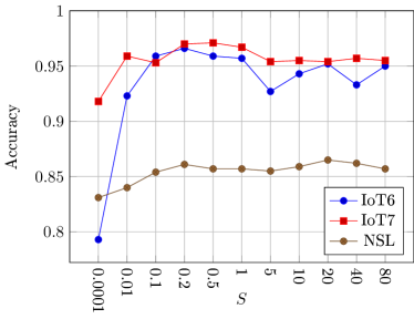
Figure 6: Influence of the scale of the transformation operator $S$.

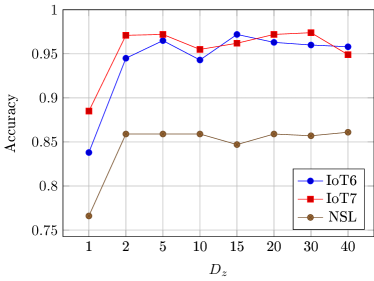
Figure 7: Influence of the size of the latent representation $D_{z}$.

For the scale of the transformation operator, $S$, we vary its value from 0.0001 to 80 and set the dimension of the latent representation $D_{z}$ at 10. The accuracy of the DT model based on TAE representation on three datasets,i.e. IoT6, IoT7, and NSL, with different values of $S$ are shown in Fig. 6. It is obvious that when the value of $S$ is too small, the accuracy of the DT model decreases. This is because when $S$ is small, the mean $\bm{\hat{\mu}}^{c}$, i.e., the mean after applying the transformation operator, of different classes is not separated (Fig. 3). For example, the accuracy obtained by DT on the IoT6 dataset is lower than 0.8 when the value of $S$ is 0.0001, which is significantly smaller than its value at 0.95 when $S$ is set to 10. When $S$ increases the accuracy of DT also increases. However, the accuracy of DT is mostly stable when $S>0.1$. This result shows that the effectiveness of TAE is not sensitive to the selection of $S$. Thus, we can set this hyper-parameter at any value greater than 0.1 to achieve the good performance of the downstream models.

The influence of the dimension of the latent vector $D_{z}$ is investigated in Fig. 7. The accuracy of the DT classifier declines when the value of $D_{z}$ is too small. For example, the accuracy of the DT classifier on NSL is lower than 0.8 when $D_{z}=1$ in comparison with the average of 0.86. The reason is that the useful information in the original data will be lost when the size of the dimension of the latent vector is too small. Moreover, the value of $D_{z}$ is not able to be greater than the dimension in the original data due to the application of PCA in Algorithm 1.

VII-E The Loss Function of TAE

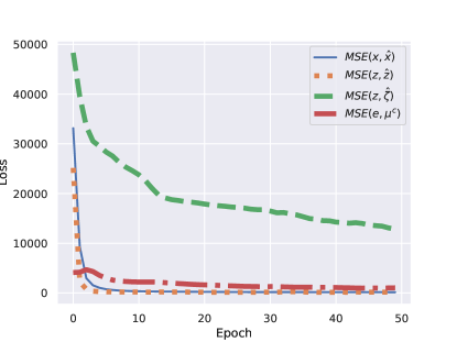
Figure 8: TAE’s loss function.

One of the questions in the training process of TAE is whether we can reconstruct the separable vector $\textbf{z}^{i}$ at the output of TAE. In other words, we would like to investigate whether the reconstruction vector is close to the separable vector. To answer this question, we conducted one more experiment to analyze the four components in the loss function of TAE. The experiment is executed on the ToT4 dataset. Fig. 8 shows the process of the four components in the loss function of TAE over 50 epochs. It is clear that the four components in the loss of TAE decrease during the training process. Among the four components, the value of the MSE score between latent space $\textbf{z}^{i}$ and its reconstruction $\hat{\textbf{z}}^{i}$ is by far greater than those of the three remaining components. This means that the loss function between $\textbf{z}^{i}$ and $\hat{\textbf{z}}^{i}$ is much harder to train. This is understandable since $\hat{\textbf{z}}^{i}$ is constructed by putting the input vector $\textbf{x}^{i}$ to the input of the TAE’s decoder and it is more difficult to force $\hat{\textbf{z}}^{i}$ close to $\textbf{z}^{i}$ compared to $\textbf{z}^{i}$ and $\hat{\textbf{z}}^{i}$. However, the figure also shows that the training process can make $\hat{\textbf{z}}^{i}$ closer to $\textbf{z}^{i}$ (although difficult) and thus in the testing phase, we can reconstruct $\textbf{z}^{i}$ by inputting the data sample to the input of the decoder of the TAE model.

VII-F Model Complexity

The last set of experiments in this section is the model complexity. We measure the mode size, i.e., the volume space the model occupies on the hard disk, in KB, and the inference time (the testing time) of TAE and compare this value with the value of MAE and Xgb. Table XIII shows these results.

TABLE XIII: Inference time and model size of TAE, MAE, and Xgb.

Metrics	Xgb	MAE	TAE
Model size (KB)	549	172	482
Avg time (seconds)	1.540E-05	1.040E-06	1.042E-06

The table shows that Xgb is the most complicated model among the three tested models. This is not surprising since Xgb is an ensemble model that aggregates a large number of decision trees. The table also shows that MAE is the simplest model and TAE is the second simplest model. For the inference time, the results in this table show that the inference time of Xgb is the highest. This is consistent with its complexity. For MEA and TAE, their inference time is mostly equal. This is because only the encoder of MEA and the decoder of TAE are used for inference and the structure of these subnetworks, i.e. the encoder of MAE and the decoder of TAE, are mostly the same.

Overall, the results in this subsection show that the model complexity of TAE is much less than that of Xgb, especially in terms of inference time. Thus, TAE is more applicable than Xgb in the domain of cybersecurity where the demand for quickly identifying attacks is critical.

VIII Assumption and Limitations

TAE was proposed based on the assumption that the diversity and sophistication of cyberattacks result in the entangle of the latent representation of AE models. Thus, TAE is more beneficial for problems where many types of different and sophisticated attacks persist. For some types of problems like binary problems or problems where the latent representation of AE models is not entangled the advantage of TAE may not be highlighted. Another situation where TAE may not be better than MAE is when the latent representation of AE can be separated by using regularized techniques.

One potential limitation of the current version of TAE is the design of the operator to transform the latent representation into the separable representation. First, this operator depends on two hyper-parameters, i.e., the direction of transformation $t$, and the scale transformation $S$. Thus, it is very important to select the appropriate values for these hyper-parameters. Second, the data samples of different classes in the separable representation may not be well discriminated if their means line in the same direction from the overall mean $\hat{\mu}$. Therefore, the transformation operator that better distinguishes the data samples in the separable space may further improve the performance of TAE.

IX Conclusions

In this paper, we proposed a novel neural network architecture called Twin Auto-Encoder (TAE) To address the challenges in detecting cyberattacks poised by their complexity and sophistication. The novelty of TAE is the transformation of the latent representation into the separable representation and the twin architecture to reconstruct the separable representation to create the reconstruction representation at the output of TAE. The reconstruction representation is then used for the downstream cyberattack detection task.

We have evaluated the performance of the proposed models using extensive experiments on a wide range of datasets including the IoT attack datasets, the network IDS datasets, the cloud DDoS dataset, and the malware datasets. The effectiveness of TAE was investigated using a popular machine learning classifier, i.e., Decision Tree (DT). Overall, the results show the superior performance of the TAE model over the state-of-the-art representation models, i.e., MAE and CSAEC. In addition, the results of TAE are also higher than those of the state-of-the-art ensemble learning method Xgb. Moreover, TAE is also better than MAE and Xgb in detecting some sophisticated and currently challenging attacks including the rare attacks in NSLKDD, the low-rate DDoS attacks in the IoT dataset, and the unknown attacks in the malware datasets. The simulation and analysis results then clearly demonstrated the superior performance of TAE.

In the future, one can extend our work in different directions. First, it is very potential to design new methods to transform the latent representation into the separable representation to boost the performance of the detection task. Second, the loss function of TAE needs to trade-off between its components. It will be better to find an approach to automatically select good values for each dataset. Last but not least, the proposed models in this article only examined the cybersecurity datasets. Therefore, it is interesting to extend this model to other fields such as computer vision and natural language processing.

References

- [1] S. Tu, M. Waqas, A. Badshah, M. Yin, and G. Abbas, “Network intrusion detection system (nids) based on pseudo-siamese stacked autoencoders in fog computing,” IEEE Transactions on Services Computing, pp. 1–12, Sept. 2023.
- [2] G. Kumar, R. Saha, M. Conti, R. Thomas, T. Devgun, and J. J. C. Rodrigues, “Adaptive intrusion detection in edge computing using cerebellar model articulation controller and spline fit,” IEEE Transactions on Services Computing, vol. 16, no. 2, pp. 900–912, May 2022.
- [3] A. L. Buczak and E. Guven, “A survey of data mining and machine learning methods for cyber security intrusion detection,” IEEE Communications Surveys & Tutorials, vol. 18, no. 2, pp. 1153–1176, Oct. 2015.
- [4] O. Y. Al-Jarrah, O. Alhussein, P. D. Yoo, S. Muhaidat, K. Taha, and K. Kim, “Data randomization and cluster-based partitioning for botnet intrusion detection,” IEEE Transactions on Cybernetics, vol. 46, no. 8, pp. 1796–1806, Aug. 2015.
- [5] I. Goodfellow, Y. Bengio, and A. Courville, Deep Learning. The MIT Press, 2016.
- [6] Y. Bengio, A. Courville, and P. Vincent, “Representation learning: A review and new perspectives,” IEEE Transactions on Pattern Analysis and Machine Intelligence, vol. 35, no. 8, pp. 1798–1828, Mar. 2013.
- [7] P. Huff, K. McClanahan, T. Le, and Q. Li, “A recommender system for tracking vulnerabilities,” in The 16th International Conference on Availability, Reliability and Security, Vienna, Austria, 2021, pp. 1–7.
- [8] S. Li, Y. Li, W. Han, X. Du, M. Guizani, and Z. Tian, “Malicious mining code detection based on ensemble learning in cloud computing environment,” Simulation Modelling Practice and Theory, vol. 113, p. 102391, Dec. 2021.
- [9] W. L. Costa, A. L. Portela, and R. L. Gomes, “Features-aware ddos detection in heterogeneous smart environments based on fog and cloud computing,” International Journal of Communication Networks and Information Security, vol. 13, no. 3, pp. 491–498, Dec. 2021.
- [10] Y. Meidan, M. Bohadana, Y. Mathov, Y. Mirsky, A. Shabtai, D. Breitenbacher, and Y. Elovici, “N-baiot—network-based detection of iot botnet attacks using deep autoencoders,” IEEE Pervasive Computing, vol. 17, no. 3, pp. 12–22, Mar. 2018.
- [11] V. Rey, P. M. S. Sánchez, A. H. Celdrán, and G. Bovet, “Federated learning for malware detection in iot devices,” Computer Networks, vol. 204, no. 1, p. 108693, Feb. 2022.
- [12] M. Tavallaee, E. Bagheri, W. Lu, and A. A. Ghorbani, “A detailed analysis of the kdd cup 99 data set,” in 2009 IEEE Symposium on Computational Intelligence for Security and Defense Applications, Ottawa, ON, Canada, 2009, pp. 1–6.
- [13] M. Al-Qatf, Y. Lasheng, M. Al-Habib, and K. Al-Sabahi, “Deep learning approach combining sparse autoencoder with svm for network intrusion detection,” IEEE Access, vol. 6, no. 1, pp. 52 843–52 856, Sept. 2018.
- [14] H. Wu and M. Flierl, “Vector quantization-based regularization for autoencoders,” in Proceedings of the AAAI Conference on Artificial Intelligence, vol. 34, no. 04, Palo Alto, California USA, 2020, pp. 6380–6387.
- [15] L. Vu, V. L. Cao, Q. U. Nguyen, D. N. Nguyen, D. T. Hoang, and E. Dutkiewicz, “Learning latent representation for iot anomaly detection,” IEEE Transactions on Cybernetics, vol. Early Access, no. 1, pp. 1–14, Sept. 2020.
- [16] N. Moustafa and J. Slay, “Unsw-nb15: a comprehensive data set for network intrusion detection systems (unsw-nb15 network data set),” in 2015 Military Communications and Information Systems Conference (MilCIS), Canberra, ACT, Australia, 2015, pp. 1–6.
- [17] S. Garcia, A. Parmisano, and M. J. Erquiaga, “Iot-23: A labeled dataset with malicious and benign iot network traffic,” Stratosphere Lab., Praha, Czech Republic, Tech. Rep, 2020.
- [18] R. Kumar, S. P. Lal, and A. Sharma, “Detecting denial of service attacks in the cloud,” in 2016 IEEE 14th Intl Conf on Dependable, Autonomic and Secure Computing, 14th Intl Conf on Pervasive Intelligence and Computing, 2nd Intl Conf on Big Data Intelligence and Computing and Cyber Science and Technology Congress (DASC/PiCom/DataCom/CyberSciTech). Auckland, New Zealand: IEEE, 2016, pp. 309–316.
- [19] W. Luo, J. Li, J. Yang, W. Xu, and J. Zhang, “Convolutional sparse autoencoders for image classification,” IEEE Transactions on Neural Networks and Learning Systems, vol. 29, no. 7, pp. 3289–3294, Jul. 2018.
- [20] T. Chen and C. Guestrin, “Xgboost: A scalable tree boosting system,” in Proceedings of the 22nd ACM SIGKDD International Conference on Knowledge Discovery and Data Mining, San Francisco California USA, 2016, pp. 785–794.
- [21] P. Vincent, H. Larochelle, I. Lajoie, Y. Bengio, and P.-A. Manzagol, “Stacked denoising autoencoders: Learning useful representations in a deep network with a local denoising criterion,” Journal of Machine Learning Research, vol. 11, no. 12, pp. 3371–3408, Dec. 2010.
- [22] G. E. Hinton and R. R. Salakhutdinov, “Reducing the dimensionality of data with neural networks,” Science, vol. 313, no. 5786, pp. 504–507, Jul. 2006.
- [23] N. Shone, T. N. Ngoc, V. D. Phai, and Q. Shi, “A deep learning approach to network intrusion detection,” IEEE Transactions on Emerging Topics in Computational Intelligence, vol. 2, no. 1, pp. 41–50, Feb. 2018.
- [24] M. Al-Qatf, Y. Lasheng, M. Al-Habib, and K. Al-Sabahi, “Deep learning approach combining sparse autoencoder with svm for network intrusion detection,” IEEE Access, vol. 6, pp. 52 843–52 856, Sept. 2018.
- [25] X. Wu and Q. Cheng, “Fractal autoencoders for feature selection,” in Proceedings of the AAAI Conference on Artificial Intelligence, vol. 35, no. 12, Vancouver, Canada, 2021, pp. 10 370–10 378.
- [26] X. Han, Y. Liu, Z. Zhang, X. Lü, and Y. Li, “Sparse auto-encoder combined with kernel for network attack detection,” Computer Communications, vol. 173, pp. 14–20, May 2021.
- [27] A. Glushkovsky, “Ai discovering a coordinate system of chemical elements: dual representation by variational autoencoders,” arXiv preprint arXiv:2011.12090, 2020.
- [28] A. Khraisat, I. Gondal, P. Vamplew, and J. Kamruzzaman, “Survey of intrusion detection systems: techniques, datasets and challenges,” Cybersecurity, vol. 2, no. 1, pp. 1–22, Jul. 2019.
- [29] M. A. Ferrag, L. Maglaras, S. Moschoyiannis, and H. Janicke, “Deep learning for cyber security intrusion detection: Approaches, datasets, and comparative study,” Journal of Information Security and Applications, vol. 50, no. 1, p. 102419, 2020.
- [30] A. V. Phan, P. N. Chau, M. Le Nguyen, and L. T. Bui, “Automatically classifying source code using tree-based approaches,” Data & Knowledge Engineering, vol. 114, pp. 12–25, Mar. 2018.
- [31] D. P. Kingma and M. Welling, “An introduction to variational autoencoders,” Foundations and Trends® in Machine Learning, vol. 12, no. 4, p. 307–392, Nov. 2019.
- [32] Y. Lu, “The level weighted structural similarity loss: A step away from mse,” in Proceedings of the AAAI Conference on Artificial Intelligence, vol. 33, no. 01, Honolulu, Hawaii, USA, 2019, pp. 9989–9990.
- [33] W. Zuo, D. Zhang, and K. Wang, “Bidirectional pca with assembled matrix distance metric for image recognition,” IEEE Transactions on Systems, Man, and Cybernetics, Part B (Cybernetics), vol. 36, no. 4, pp. 863–872, Aug. 2006.
- [34] D. P. Kingma and J. Ba, “Adam: A method for stochastic optimization,” in ICLR (Poster), 2015.
- [35] M. Li, T. Zhang, Y. Chen, and A. J. Smola, “Efficient mini-batch training for stochastic optimization,” in Proceedings of the 20th ACM SIGKDD International Conference on Knowledge Discovery and Data Mining, New York, United States, Aug. 2014, pp. 661–670.
- [36] M. Sokolova, N. Japkowicz, and S. Szpakowicz, “Beyond accuracy, f-score and roc: a family of discriminant measures for performance evaluation,” in Australasian joint conference on artificial intelligence. Springer, 2006, pp. 1015–1021.
- [37] Y. Yu and N. Bian, “An intrusion detection method using few-shot learning,” IEEE Access, vol. 8, pp. 49 730–49 740, Mar. 2020.
- [38] J. Park, J. Lee, and D. Sim, “Low-complexity cnn with 1d and 2d filters for super-resolution,” Journal of Real-Time Image Processing, vol. 17, no. 6, pp. 2065–2076, Jun. 2020.
- [39] Y. Yin, J. Jang-Jaccard, W. Xu, A. Singh, J. Zhu, F. Sabrina, and J. Kwak, “Igrf-rfe: a hybrid feature selection method for mlp-based network intrusion detection on unsw-nb15 dataset,” Journal of Big Data, vol. 10, no. 1, pp. 1–26, Feb. 2023.
- [40] F. Pedregosa, G. Varoquaux, A. Gramfort, V. Michel, B. Thirion, O. Grisel, M. Blondel, P. Prettenhofer, R. Weiss, V. Dubourg et al., “Scikit-learn: Machine learning in python,” Journal of Machine Learning Research, vol. 12, pp. 2825–2830, Feb. 2011.
- [41] A. Jain, K. Nandakumar, and A. Ross, “Score normalization in multimodal biometric systems,” Pattern Recognition, vol. 38, no. 12, pp. 2270–2285, Dec. 2005.
- [42] M. Azizjon, A. Jumabek, and W. Kim, “1d cnn based network intrusion detection with normalization on imbalanced data,” in 2020 International Conference on Artificial Intelligence in Information and Communication (ICAIIC). Fukuoka, Japan: IEEE, 2020, pp. 218–224.
- [43] X. Glorot and Y. Bengio, “Understanding the difficulty of training deep feedforward neural networks,” in Proceedings of the Thirteenth International Conference on Artificial Intelligence and Statistics. Chia Laguna Resort, Sardinia, Italy: JMLR Workshop and Conference Proceedings, 2010, pp. 249–256.
- [44] P. V. Dinh, N. Q. Uy, D. N. Nguyen, D. T. Hoang, S. P. Bao, and E. Dutkiewicz, “Twin variational auto-encoder for representation learning in iot intrusion detection,” in 2022 IEEE Wireless Communications and Networking Conference (WCNC). Austin, TX, USA: IEEE, 2022, pp. 848–853.
- [45] V. L. Cao, M. Nicolau, and J. McDermott, “Learning neural representations for network anomaly detection,” IEEE Transactions on Cybernetics, vol. 49, no. 8, pp. 3074–3087, Jun. 2019.
- [46] C. Xiang, P. C. Yong, and L. S. Meng, “Design of multiple-level hybrid classifier for intrusion detection system using bayesian clustering and decision trees,” Pattern Recognition Letters, vol. 29, no. 7, pp. 918–924, May 2008.
- [47] P. Xanthopoulos, P. M. Pardalos, T. B. Trafalis, P. Xanthopoulos, P. M. Pardalos, and T. B. Trafalis, “Linear discriminant analysis,” Robust Data Mining, pp. 27–33, Jan. 2013.