Single-token vs Two-token Blockchain Tokenomics

Abstract

We consider long-term equilibria that arise in the tokenomics design of proof-of-stake (PoS) blockchain systems that comprise of users and validators, both striving to maximize their own utilities. Validators are system maintainers who get rewarded with tokens for performing the work necessary for the system to function properly, while users compete and pay with such tokens for getting a desired system service level.

We study how the system service provision and suitable rewards schemes together can lead to equilibria with desirable characteristics (1) viability: the system keeps parties engaged, (2) decentralization: multiple validators are participating, (3) stability: the price path of the underlying token used to transact with the system does not change widely over time, and (4) feasibility: the mechanism is easy to implement as a smart contract, i.e., it does not require fiat reserves on-chain for buy back of tokens or to perform bookkeeping of exponentially growing token holdings. Furthermore, we consider both the common single-token PoS model and a less widely used two-token approach (that roughly, utilizes one token for the users to pay the transaction fees and a different token for the validators to participate in the PoS protocol and get rewarded). Our approach demonstrates, for the first time to our knowledge, concrete advantages of the two-token approach in terms of the ability of the mechanism to reach equilibrium.

1 Introduction

Designing tokenomics policies with good properties is pivotal to ensuring the success of blockchain systems in the long term. Blockchains create value by offering services in a fully decentralized manner, wherein users pay fees to access these services, while the functioning and security of the system is guaranteed by a set of nodes or validators who receive rewards for performing the necessary computations required by the protocol. These payments are issued in the system’s native token. The token’s value or price, denoted in standard (fiat) currency, crucially determines the actual costs for users and the compensation for validators. A drop or fluctuation in the token’s price can make the system less attractive for both types of parties. While the system cannot directly control its token price in the market, it can implement various monetary policies (such as token minting, adjusting the total supply or transaction fees, change the validator rewards mechanisms, and others) to achieve a long-term equilibrium with the desired price without compromising the system’s viability and decentralization.

This motivates the study of tokenomics designs achieving the following important desiderata:

1. Viability. The system that keeps all involved parties actively engaged: validators to guarantee the protocol being alive and securely running, and the users to guarantee enough fees are collected at all time.

2. Decentralization. A set of validators each equally engaged in the protocol, receiving adequate rewards, while also having significant stake in the system operation (e.g. in the case of proof-of-stake (PoS) systems, validators “staking” high enough amount of tokens).

3. Stability. Reasonably stable token prices, meaning that the price of the token required to issue transactions over time does not change or does not become inflationary (decreasing prices).

4. Feasibility. The tokenomics policy should be feasible to implement on-chain algorithmically. In particular, this means that the policy avoids using features that are incompatible or difficult to implement in the form of smart contracts, integrate into the accounting model or they are antithetical to blockchain decentralization. For example, the policy should minimize the use of off-chain entities that need to be consulted on-chain as “oracles” or the use of techniques such as buy-backs which require the use of fiat reserves to facilitate them. Furthermore, all the numerical quantities that are accounted in the ledger (e.g., the number of tokens held by a validator) should not grow exponentially over time.

The conditions under which there is a tokenomics policy achieving all these requirements is a fundamental question which we address in this work.

1.1 Main contributions

We explore tokenomics policies in the PoS setting, i.e., the setting where validators have to acquire tokens and stake them in order to receive rewards and perform the necessary system maintenance to further the system’s operation. We put forth a model where a set of $m$ users and $n$ validators engage with the system in discrete time steps. At each time step, users and validators buy or sell tokens in order to accommodate their objectives that include issuing transactions and staking tokens to provide the service.

We give both boundary conditions and actual policies (mechanisms) that implement equilibria with all desired features: viability, decentralization, stability, and feasibility. Specifically, the resulting mechanism only needs to adjust the total rewards allocated to the validators in the next round, though it does so in a somewhat counterintuitive way:

If the demand for tokens drops, instead of buying back tokens, the mechanism increases the rewards allocated to validators.

This idea steams from our analysis of equilibria that maintain a given price path (e.g., stable prices):

• Prices and equilibria. We show that, in all equilibria implementing certain desired price paths, at every epoch or round (i) users spend a constant fraction of the total value of the offered service, and (ii) validators stake a constant fraction of the total rewards offered by the system (Theorem 1).

The main catch here is that these two quantities are not necessarily related to each other, and the system can actually adjust the rewards in order to match changes in the value of the service, and keep the desired prices without performing token buy backs. If, at any point in time, the value of the service level decreases, users will buy fewer tokens, thereby reducing demand and potentially necessitating token buybacks. Rather than engaging in token buybacks, the system can opt to increase the rewards allocated to validators. As validators compete for the rewards, they react by staking more tokens, which they must acquire from the market. This action effectively restores the demand for tokens to align with the supply and avoids buybacks.

• Single Token Equilibria. We provide a mechanism which adjusts the rewards at every round based on the current rewards and the next round service value using a single token for accounting. In order for this mechanism to work, and keep the token rewards and staked holdings under control for feasibility, the mechanism needs to have some global information about the service value time series (e.g., a lower bound, cf. Theorem 2 and Corollary 2).

Intuitively, the mechanism strives to use the largest possible rewards (so to guarantee decentralization and security – a good margin for the validators profit), while not exceeding at any point in time the value which triggers an uncontrolled growth in the rewards and in the staked amounts of tokens (Section 3.3.1). In other words, the mechanism provides the highest possible rewards (i.e., decentralization and security guarantee) while satisfying the other three desiderata (viable system, stable prices, no buy backs). In Section 3.4 we describe in detail the implementation of our mechanism for the case of stable prices. This implementation includes the strategies for users and validators, showing that all information needed is the next round service level offered by the system (despite their simplicity, these strategies still constitute an equilibrium in the underlining repeated game, i.e., when more complex time-dependent strategies are in principle possible).

The above results apply to a single token setting which is the most common in PoS systems (e.g., Ethereum and Cardano operate in this way among the top cryptocurrencies). We next explore the setting of two token PoS in which one token is used to get the service and another token is used for staking (and governance). While less popular, this type of setup has been adopted in the Neo cryptocurrency and can be implemented in other systems as well (e.g., in the Cosmos SDK). To investigate the potential of these mechanisms, we introduce a natural variant of our model with two tokens. In order to maintain feasibility and avoid buy backs, while maintaining desirable prices, we identify the necessary conditions that equilibria (mechanism) must guarantee in terms of rewards:

• Double Token Equilibira. The two token mechanism is presented in Section 4.3. The main advantage of the resulting rewards formula is that it is simpler than in the single token setting and the mechanism does not need to know “global information” about the service value time series — merely a one step lookahead suffices (cf. Theorem 4). As a result, the mechanism achieves our objectives with less information about the service value time series.

Intuitively, the advantage of “decoupling” the users from the validators, using different tokens, allows to better react and absorb shocks and fluctuations in the value of the service while maintaining the price of the users’ token stable and keeping all our feasibility desiderata. The price of the token used for staking increase “gradually”, while the amount of staked tokens remains constant, without scarifying incentive compatibility. Hence, the security of the protocol is preserved (the value of the staked tokens increases). This should be compared and contrasted with the single-token mechanism, which either (i) needs to know a global property of the service level time series, or in any case, be informed well in advance about a sudden drop in service value in order to be able to gradually decrease the rewards (as it can only adjust the rewards according to a certain “decreasing curve”), or (ii) it should proactively keep rewards well below the possible value (thus achieving a suboptimal security level for the protocol).

Related work. In the single-token setting, our results build on the model of Häfner (2023). Compared to that prior work, our results accommodate a more general class of equilibria with respect to their features, that facilitate stable prices without the requirement to employ buy backs. To the best of our knowledge, ours is the first analytical model for such systems to study their equilibria and related token price paths achieving all four desiderata. Prior work includes the effects of tokens regarding user adoption and equilibrium section Bakos and Halaburda (2019, 2022); Sockin and Xiong (2023); Li and Mann (2018), or using token supply and buyback to promote optimal growth and service provision Cong et al. (2021, 2022). Different aspects of the monetary characteristics of tokens have been studied in Schilling and Uhlig (2019); Pagnotta (2022); Prat et al. (2021), while Kiayias et al. (2023) considered token burning. Typically the users receive the most modelling attention, but Chitra (2021) expand on the strategy space of validators and their alternative uses for tokens. While all previous work has focused on the single token design, Dimitri (2023) has considered a two-token model.

2 Model description and notation (single token)

Notation (single token model)

• $m$ = number of users (fixed and constant over time) • $n$ = number of validators (fixed and constant over time) • $\mathbb{TK}_{p}$ = token holding of a generic player $p$ (user or validator) • $\mathbb{PRICE}$ = price of the token • $f^{(t)}$ the value of a generic quantity $f$ at time $t$ • $f^{(\delta,\infty)}$ = discounted version of quantity $f^{(t)}$, that is, $f^{(\delta,\infty)}=\sum_{t=0}^{\infty}\delta^{t}f^{(t)}$ • $f^{(\delta,\infty|t)}$ = generalization of the previous definition in which we start at $t$ and discount accordingly, that is, $f^{(\delta,\infty|t)}=\sum_{\tau=t}^{\infty}\delta^{\tau-t}f^{(\tau)}=f^{(t)}+\delta f^{(\delta,\infty|t+1)}$ • $s_{j}^{(t)}$ = validator $j$’s selling strategy at time $t$ (negative values are possible, i.e., buying) • $b_{i}^{(t)}$ = user $i$’s buying strategy at time $t$ (negative values are possible, i.e., selling) • $u_{i}^{(t)}$ = amount of tokens that user $i$ pays for the service at time $t$ • $v$ = cost incurred by each validator (identical for all validators and all $t$ as in Häfner (2023)) • $R^{(t)}$ is the total reward for validators at time $t$, which is further distributed to each validator according to a reward sharing scheme $r(\cdot)$, meaning that validator $j$ receives an amount of tokens equal to $\displaystyle R_{j}^{(t)}:=R^{(t)}\cdot r(\mathbb{TK}_{j}^{(t)},\mathbb{TK}_{-j}^{(t)})$ (1) where $\mathbb{TK}_{-j}^{(t)}$ are the token holding of all validators but $j$. • $S^{(t)}$ is the service level at time $t$, which is further assigned to each users according to some scheme $s(\cdot)$, meaning that each user $i$ receives a service level $\displaystyle S_{i}^{(t)}:=S^{(t)}\cdot s(u_{i}^{(t)},u_{-i}^{(t)})$ (2) where $u_{-i}^{(t)}$ are the used tokens of all users but $i$. • $g(n)$ = generic non-decreasing decentralization factor, where $n$ is the number of validators • $U_{i}^{(t)}$ = instantaneous utility of user $i$, given by $\displaystyle U_{i}^{(t)}=S_{i}^{(t)}\cdot g(n)-b_{i}^{(t)}\cdot\mathbb{PRICE}^{(t)}$ (3) • $V_{j}^{(t)}$ = instantaneous utility of validator $j$, given by $\displaystyle V_{j}^{(t)}=s_{j}^{(t)}\cdot\mathbb{PRICE}^{(t)}-v$ (4)

Figure 1: Notation and symbols.

In order to describe the model in detail, we introduce some notation in Figure 1. We have a repeated game with discount factor $\delta$ where each round $t$ consists of the following two subrounds, where players first interact with the system (pay & stake with tokens) and then they interact with the “market” (buy or sell tokens):

Subround I (pay & stake):

Each user $i$ and each validator $j$ has $\mathbb{TK}_{i}^{(t)}$ and $\mathbb{TK}_{j}^{(t)}$ tokens, respectively. Then:

1. Each validator $j$ performs some work, incurs a cost $v$, and receives an amount $R_{j}^{(t)}$ of additional tokens according to (1).

2. Each user $i$ uses some of her currently available tokens to pay for the service, and receives the corresponding service level according to (2).

Subround II (buy or sell):

Each user $i$ and each validator $j$ has $\mathbb{TK}_{i}^{(t)}-u_{i}^{(t)}$ and $\mathbb{TK}_{j}^{(t)}+R_{j}^{(t)}$ tokens, respectively. Both type of players (users and validators) can buy any amount of new tokens or sell (part or all of the tokens they currently have) at the current market price. In detail:

1. Each validator $j$ sells $s_{j}^{(t)}$ tokens to the market and receives $s_{j}^{(t)}\cdot\mathbb{PRICE}^{(t)}$ units of money in return. Note that we have a validator’s selling constraint

   $$s_{j}^{(t)}\leq\mathbb{TK}_{j}^{(t)}+R_{j}^{(t)}\ .$$ (5)

   Any negative $s_{j}^{(t)}$ is allowed meaning that $j$ is actually buying tokens from the market at the current price.

2. Each user $i$ buys $b_{i}^{(t)}$ additional tokens from the market and pays $b_{i}^{(t)}\cdot\mathbb{PRICE}^{(t)}$ units of money for that. Any negative $b_{i}^{(t)}$ is allowed, meaning that $i$ is selling tokens to the market at the current price. Note that we have a users’s selling constraint

   $$-b_{i}^{(t)}\leq\mathbb{TK}_{i}^{(t)}-u_{i}^{(t)}\ .$$ (6)

At the end of subround II of step $t$ we get the token holdings for the next step, $t+1$, for each user $i$ and each validator $j$, respectively

$$\mathbb{TK}_{i}^{(t+1)}=\mathbb{TK}_{i}^{(t)}-u_{i}^{(t)}+b_{i}^{(t)}\stackrel{{\scriptstyle\eqref{eq:usr-sell-constraint}}}{{\geq}}0 \mathbb{TK}_{j}^{(t+1)}=\mathbb{TK}_{j}^{(t)}+R_{j}^{(t)}-s_{j}^{(t)}\stackrel{{\scriptstyle\eqref{eq:val-sell-constraint}}}{{\geq}}0\ .$$ (7)

Each user $i$ and each validator $j$ aims at maximizing her own discounted utility, respectively

$$U_{i}^{(\delta,\infty)} \stackrel{{\scriptstyle\eqref{eq:usr-utility-istant}}}{{=}}\sum_{t=0}^{\infty}\delta^{t}\cdot[S_{i}^{(t)}\cdot g(n)-b_{i}^{(t)}\cdot\mathbb{PRICE}^{(t)}]\,$$ (8)

$$V_{j}^{(\delta,\infty)} \stackrel{{\scriptstyle\eqref{eq:val-utility-istant}}}{{=}}\sum_{t=0}^{\infty}\delta^{t}\cdot[s_{j}^{(t)}\cdot\mathbb{PRICE}^{(t)}-v]$$ (9)

subject to their respective selling constraints in (6) and in (5).

Definition 1 (symmetric equilibrium).

Consider a system policy given by (1) and (2), and a triple of users’ strategies, validators’ strategies, and prices

$$(u_{i}^{(t)},b_{i}^{(t)}) s_{j}^{(t)} \mathbb{PRICE}^{(t)}$$ (10)

such that the corresponding selling constraints (6) and (5) are satisfied. We say that such a triple is an equilibrium if

1. Strategy $s_{j}^{(t)}$ maximizes the discounted utility (9) of validator $j$, given all other strategies, for each validator $j$;

2. Strategy $(u_{i}^{(t)},b_{i}^{(t)})$ maximizes the discounted utility (8) of user $i$, given all other strategies, for each user $i$;

3. The resulting two sequences of token holdings (7) are strictly positive, that is, $\mathbb{TK}_{i}^{(t)}>0$ and $\mathbb{TK}_{j}^{(t)}>0$.

Moreover, we say that such an equilibrium is symmetric if the token holdings of all users are the same, and similarly, if all token holdings of all validators are the same, correspond to sequences of strictly positive token holdings

$$\mathbb{TK}_{i}^{(t)}=\mathbb{TK}_{U}^{(t)}>0 \mathbb{TK}_{j}^{(t)}=\mathbb{TK}_{V}^{(t)}>0\ .$$ (11)

for all users $i$ and for all validators $j$ and for all $t$.

Remark 1.

The condition that tokens holding must be strictly positive at all time steps is identical to the definition of equilibrium in Häfner (2023). In particular, it implies that the selling/buying strategies at such an equilibrium satisfy the selling constraints (6) and (5) with a strict inequality.

Remark 2.

The results in Häfner (2023) mostly focus on equilibria that have two additional conditions, namely, validators hold a constant fraction of all tokens (constant staking),

$$\frac{n\mathbb{TK}_{V}^{(t)}}{m\mathbb{TK}_{U}^{(t)}+n\mathbb{TK}_{V}^{(t)}}=\rho>0$$ (12)

and the reward is also a fraction of all current tokens (constant inflation from validation)

$$\frac{R^{(t)}}{m\mathbb{TK}_{U}^{(t)}+n\mathbb{TK}_{V}^{(t)}}=I>0$$ (13)

Lemma 1.

(Häfner, 2023, Lemma 1) For the following special case of reward sharing and service schemes,

$$S_{i}^{(t)}=S^{(t)}\cdot\left(\frac{u_{i}^{(t)}}{\sum_{k}u_{k}^{(t)}}\right) R_{j}^{(t)}=R^{(t)}\cdot\left(\frac{\mathbb{TK}_{j}^{(t)}}{\sum_{v}\mathbb{TK}_{v}^{(t)}}\right)$$ (14)

where $k$ and $v$ range over all users and all validators, respectively, the following holds. In any symmetric equilibrium

$$\mathbb{PRICE}^{(t-1)}=\mathbb{PRICE}^{(t)}\cdot\delta\cdot\left(1+\frac{I}{\rho}\cdot\frac{n-1}{n}\right)$$ (15)

In the next section we generalize the price analysis above to a more general class of reward and service sharing schemes, and without imposing the constant staking and constant inflation from validation conditions in Remark 2.

In order to establish the existence of equilibria, we need a few (technical) assumptions that are also satisfied in the setting by Häfner (2023). The first one below is about the service level, and another is on the rewards and service sharing functions.

Assumption 1 (service levels).

The service level $S^{(t)}$ is upper bounded by some (arbitrarily large) constant independent of $t$.

The value of the constant in Assumption 1 does not affect the results and bounds in any way, and is only needed to establish the existence of equilibria. Other than this, we make no other assumptions, and allow $S^{(t)}$ to increase or decrease arbitrarily within this range. Häfner (2023) considers a setting where $S^{(t)}$ can be chosen by the system, though the system incurs some quadratic time-dependent cost, and the equilibria maximizing the profit of the system in this setting will set $S^{(t)}$ so to satisfy Assumption 1. Our results apply to a more general setting, including the cases where $S^{(t)}$ is some exogenous quantity that the system cannot directly control, but can only react to it by changing other parameters, e.g., the rewards $R^{(t)}$.

3 Single token mechanisms

3.1 Analysis of price path

In this section we generalize the result in Lemma 1. Consider the following family of service allocation and rewards:

$$S_{i}^{(t)}=S^{(t)}\cdot s\left(\frac{u_{i}^{(t)}}{\sum_{k}u_{k}^{(t)}}\right) R_{j}^{(t)}=R^{(t)}\cdot r\left(\frac{\mathbb{TK}_{j}^{(t)}}{\sum_{v}\mathbb{TK}_{v}^{(t)}}\right)$$ (16)

where $s(\cdot)$ and $r(\cdot)$ are arbitrary differentiable functions in $(0,1)$, and where the indexes $k$ and $v$ in the summations range over all users and all validators, respectively. In the following, we denote by $r^{\prime}(\cdot)$ and $s^{\prime}(\cdot)$ the first derivatives of $r(\cdot)$ and $s(\cdot)$, respectively. We make the following assumption about $r(\cdot)$ and $s(\cdot)$.

Assumption 2.

We assume that the functions $r(\cdot)$ and $s(\cdot)$ in (16) are both concave. Moreover, for the number $m\geq 2$ and $n\geq 2$ of users and validators under consideration, they never allocate more than the total rewards or service available, $r(1/n)\leq 1/n$ and $s(1/m)\leq 1/m$, and the first derivatives satisfy $r^{\prime}(1/n)>0$ and $s^{\prime}(1/m)>0$.

The proof of this result follows the same arguments in Häfner (2023).

Lemma 2.

In any symmetric equilibrium, it holds that

$$\mathbb{PRICE}^{(t-1)}=\mathbb{PRICE}^{(t)}\cdot\delta\cdot\mathcal{R}^{(t)}\ . \mathcal{R}^{(t)}=1+\frac{R^{(t)}}{n\mathbb{TK}_{V}^{(t)}}\cdot\frac{n-1}{n}\cdot r^{\prime}(\frac{1}{n})\ .$$ (17)

Moreover

$$\mathbb{PRICE}^{(t-1)}=\delta\cdot\begin{cases}\mathcal{S}^{(t)}&\text{if }u_{i}^{(t)}=\mathbb{TK}_{U}^{(t)}\\ \mathbb{PRICE}^{(t)}&\text{if }u_{i}^{(t)}<\mathbb{TK}_{U}^{(t)}\end{cases}\ , \mathcal{S}^{(t)}=\frac{S^{(t)}}{m\mathbb{TK}_{U}^{(t)}}\cdot g(n)\cdot\frac{m-1}{m}\cdot s^{\prime}(\frac{1}{m})\ .$$ (18)

Hence, if $\mathcal{R}^{(t)}\neq 1$, then $u_{i}^{(t)}=\mathbb{TK}_{U}^{(t)}$ and $b_{i}^{(t)}=\mathbb{TK}_{U}^{(t+1)}$ for all users $i$, and the following identity must hold:

$$\mathbb{PRICE}^{(t)}\mathcal{R}^{(t)}=\mathcal{S}^{(t)}$$ (19)

We next provide an example of a possible reward sharing function $r(\cdot)$ other than the one in (14). We do not claim that this alternative $r(\cdot)$ provides any particular improvement, but simply point out that changing $r(\cdot)$, and similarly $s(\cdot)$, does affect the equilibria as described by Lemma 2. Appendix B describes another example of $r(\cdot)$.

Example 1.

For any parameter $\ell>1$, the following reward sharing function $r(x)=x-x^{\ell}$ satisfies $r(1/n)=1/n-1/n^{\ell}>0$, meaning that for smaller number of validators a smaller fraction of the total allocated rewards is actually distributed. Since $r^{\prime}(1/n)=1-\ell/n^{\ell-1}$, we have $r^{\prime}(1/n)>0$ for sufficiently large $n$.

Remark 3.

Assumption 2 implies that $\mathcal{R}^{(t)}>1$ whenever $R^{(t)}>0$, thus implying that the largest possible price growth must satisfy $\mathbb{PRICE}^{(t)}<\mathbb{PRICE}^{(t-1)}/\delta=(1+r)\cdot\mathbb{PRICE}^{(t-1)}$ where $\delta=1/(1+r)$ and $r$ is the risk-free rate. Intuitively, the return rate for just holding the token cannot beat the risk-free rate, as one might expect when looking for equilibria that keep all users and validators engaged (viability). Whether blockchains can achieve return rates competitive with the inflation is studied in Félez-Viñas et al. (2021) in relation to policies adopted by some of the current blockchains, though without providing analytical results.

3.2 Generic symmetric equilibria

In the following we focus on the interesting case of prices having a constant multiplicative growth, that is, for all $t\geq 1$

$$\mathbb{PRICE}^{(t)}=\frac{1}{\gamma}\cdot\mathbb{PRICE}^{(t-1)} \gamma\neq\delta,\ \gamma>0\ .$$ (20)

Note that stable prices satisfy the above condition with $\gamma=1$, while $\gamma>1$ and $\gamma<1$ corresponds to decreasing and increasing prices, respectively.

We next define a class of generic symmetric equilibria which, as we prove below, captures all symmetric equilibria whose prices follow the above path (20).

Definition 2 (generic symmetric equilibrium).

A symmetric equilibrium is generic if the following conditions hold for all $t\geq 1$:

1. The monetary amount of tokens that users hold (and use) is proportional to the service level offered by the system. That is, the service to fees ratio is constant,

   $$Ser2Fees^{(t)}:=\frac{S^{(t)}}{m\mathbb{TK}_{U}^{(t)}\cdot\mathbb{PRICE}^{(t)}}=Ser2Fees\ .$$ (21)

2. The amount of tokens staked by validators is proportional to the rewards offered by the system. That is, the rewards to stake ratio is constant,

   $$Rew2Stake^{(t)}:=\frac{R^{(t)}}{n\mathbb{TK}_{V}^{(t)}}=Rew2Stake\ .$$ (22)

3. The prices satisfy

   $$\mathbb{PRICE}^{(t-1)}= \delta\cdot\mathbb{PRICE}^{(t)}\cdot(1+Rew2Stake\cdot\kappa_{R})$$ (23)

   $$= \delta\cdot\mathbb{PRICE}^{(t)}\cdot Ser2Fees\cdot\kappa_{S}$$ (24)

   where constants $\kappa_{R}$ and $\kappa_{S}$ depend only on the number of users $m$, the number of validators $n$, the rewards sharing scheme, and on the service fee scheme.

4. Each user $i$ starts round $t$ with the same token holding $\mathbb{TK}_{U}^{(t)}$, uses all its token current holding for the service ($u_{i}^{(t)}=\mathbb{TK}_{U}^{(t)}$), and buys new tokens needed for the next round accordingly ($b_{i}^{(t)}=\mathbb{TK}_{U}^{(t+1)}$).

Note that generic symmetric equilibria provide additional structure to the definition of symmetric equilibria. The following theorem says that we can restrict to generic symmetric equilibria without loss of generality as long as we want prices with a multiplicative growth (20), e.g., stable prices.

Theorem 1.

Any symmetric equilibrium for the reward and service fee schemes in (16) whose prices satisfy (20) is a generic symmetric equilibrium with constants

$$\kappa_{R}=\frac{n-1}{n}\cdot r^{\prime}(1/n) \kappa_{S}=g(n)\cdot\frac{m-1}{m}\cdot s^{\prime}(1/n)\ .$$ and (25)

This in particular holds true for the case of stable prices.

Note that stable prices require the following specific constants in the two ratios involving the tokens:

$$Ser2Fees=1/(\delta\kappa_{S}) Rew2Stake=(1-\delta)/(\delta\kappa_{R})$$ (26)

thus implying that it must hold $\kappa_{R}>0$ and $\kappa_{S}>0$.

Corollary 1.

Any generic symmetric equilibrium (and thus any symmetric equilibrium for the reward and service fee schemes in (16)) with stable prices must have the following token holdings:

$$\mathbb{TK}_{U}^{(t)}=\frac{S^{(t)}}{m}\cdot\delta\cdot\kappa_{S}>0 \mathbb{TK}_{V}^{(t)}=\frac{R^{(t)}}{n}\cdot\frac{\delta}{1-\delta}\cdot\kappa_{R}>0$$ and (27)

for any nonnegative $S^{(t)}$ and $R^{(t)}$.

3.3 No buy back condition and its implications

Like in the original model by Häfner (2023), in the model considered so far the system is allowed to buy or to sell the additional tokens required during each subround II to match demand with supply. In this section, we refine the concept of equilibrium, by requiring that the system does not have to buy back tokens (and perhaps does not sell tokens either if demand and suppy match at equilibrium).

Definition 3 (no buy back).

We say that a symmetric equilibrium satisfies the no buy back condition if no additional tokens are bought at any round by the system, that is, $mb_{U}^{(t)}\geq ns_{V}^{(t)}$ for all $t$.

Intuitively speaking, the following theorem says that increasing the rewards at the next round does help for the no buy back condition. The intuitive, though perhaps surprising, reason is that this will make rewards more attractive for the validators who then stake more tokens (and thus sell less on the market).

Theorem 2.

In any generic symmetric equilibrium, the no buy back condition holds at round $t$ if and only if the rewards satisfy the following condition

$$R^{(t+1)}\geq R^{(t)}\cdot(1+a)-b\cdot S^{(t+1)}\cdot(\delta\mathcal{R})^{t+1}$$ (28)

where

$$a=Rew2Stake\cdot n\cdot r(1/n)\ , b=\frac{Rew2Stake}{Ser2Fees}\cdot\frac{1}{\mathbb{PRICE}^{(0)}}\ , \mathcal{R}=1+Rew2Stake\cdot\kappa_{R}\ .$$ (29)

Proof.

Let us first observe that the total amount of tokens bought by the users (demand) is

$$mb_{U}^{(t)}=m\mathbb{TK}_{U}^{(t+1)}=\frac{S^{(t+1)}}{\mathbb{PRICE}^{(t+1)}\cdot Ser2Fees}=\frac{S^{(t+1)}\cdot(\delta\mathcal{R})^{t+1}}{\mathbb{PRICE}^{(0)}\cdot Ser2Fees}$$

where $\mathcal{R}=1+Rew2Stake\cdot\kappa_{R}$. The total amount of tokens sold by the validators (supply) is

$$ns_{V}^{(t)} =n\left(\mathbb{TK}_{V}^{(t)}-\mathbb{TK}_{V}^{(t+1)}+R^{(t)}\cdot r(1/n)\right)=\frac{R^{(t)}}{Rew2Stake}-\frac{R^{(t+1)}}{Rew2Stake}+R^{(t)}\cdot n\cdot r(1/n)\ .$$

Hence, the no buy back condition $mb_{U}^{(t)}\geq ns_{V}^{(t)}$ is equivalent to

$$\frac{R^{(t)}}{Rew2Stake}-\frac{R^{(t+1)}}{Rew2Stake}+R^{(t)}\cdot n\cdot r(1/n)\leq\frac{S^{(t+1)}\cdot(\delta\mathcal{R})^{t+1}}{\mathbb{PRICE}^{(0)}\cdot Ser2Fees}$$

that is

$$R^{(t)}-R^{(t+1)}+R^{(t)}\cdot n\cdot r(1/n)\cdot Rew2Stake\leq\frac{Rew2Stake}{\mathbb{PRICE}^{(0)}\cdot Ser2Fees}\cdot S^{(t+1)}\cdot(\delta\mathcal{R})^{t+1}\ .$$

By rearranging the terms, the theorem follows. ∎

The above theorem provides a recursive (algorithmic) formula for the rewards, which leads to our mechanism described in Section 3.4 below. The same theorem also implies the following bound on the growth of the rewards necessary to guarantee the no buy back.

Corollary 2.

The minimal rewards satisfying the no buy back condition tightly are equal to

$$R_{single}^{(t+1)}=(1+a)^{t}\cdot\left(R^{(0)}-b\sum_{\tau=1}^{t}S^{(\tau)}{}\cdot\left(\frac{\delta\mathcal{R}}{1+a}\right)^{\tau}\right)\ , t\geq 1$$ (30)

for any initial reward $R^{(0)}$, and for constants $a$, $b$, and $\mathcal{R}$ as in Theorem 2.

3.3.1 Main dilemma: Uncontrolled growth of rewards

The bound in Corollary 2 suggests that an exponential growth of the rewards over time is necessary if the system starts with a too high initial reward or the service level is too low.

In the following experiment, we consider constant service level and rewards that are set to the minimal value necessary in order to have no buy back (Theorem 2), and also impose the rewards to not be below some minimum value (set to 0.1 for the sake of exposition). For the sake of simplicity, we consider the rewards and cost sharing schemes in (14) and $g(n)=1$, and observe the following:

• Sufficiently high service level can avoid rewards explosion (Figure 2 compares two different service levels under the same conditions). The necessary increase in the service level max simply be not possible due to inherent technological limitations.

• Sufficiently small initial rewards also avoid the rewards explosion (Figure 3 compares two initial rewards under the same conditions). Rewards however cannot be arbitrarily small since they must cover the costs of validators and be competitive against other source of investments.

• A higher risk free rate may also trigger an exponential growth (Figure 4 shows that for smaller $\delta$ we need a smaller initial reward, or a larger service level, to avoid this explosion).

• Allowing the token price to decrease does avoid the rewards explosion that instead occur with stable prices, once we consider the rewards in money (Figure 5). Decreasing prices are however not desirable, and perhaps one may want increasing prices, which turn out to make the monetary reward explosion even more severe.

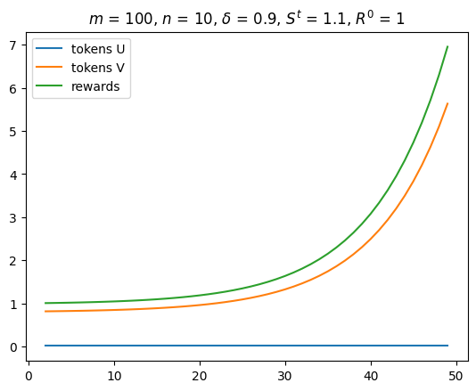
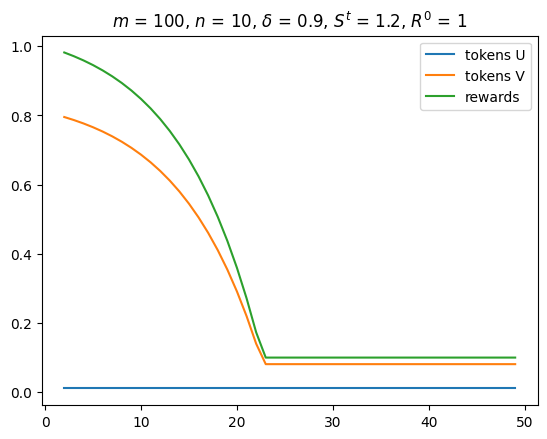
Figure 2: The effect of service level on rewards growth when no buy back condition: a small service level (left) can trigger an exponential increase in both rewards and validators staked amounts, while a slightly bigger service level (right) can remove this growth.

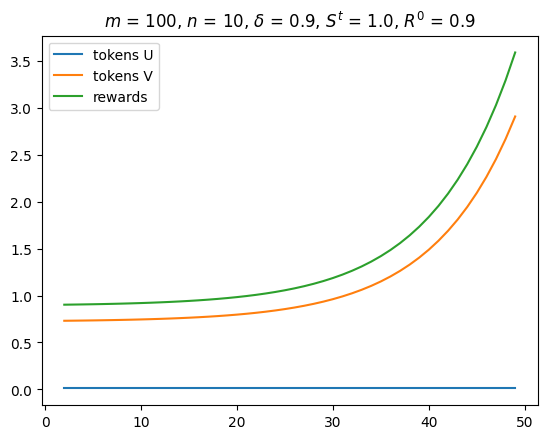
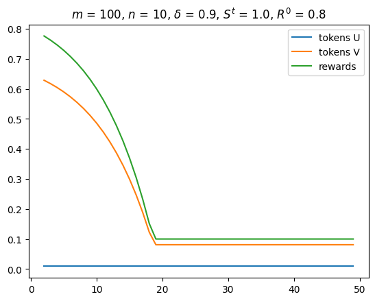
Figure 3: A too high initial rewards (left) causes an exponential growth, as opposed to a smaller initial rewards (right) leading to stable rewards and staked tokens (note the different scale of the y-axis in the two plots). In both cases, we fix a minimum value of $0.1$ for the rewards, which is the flat part of the green line in the right plot.

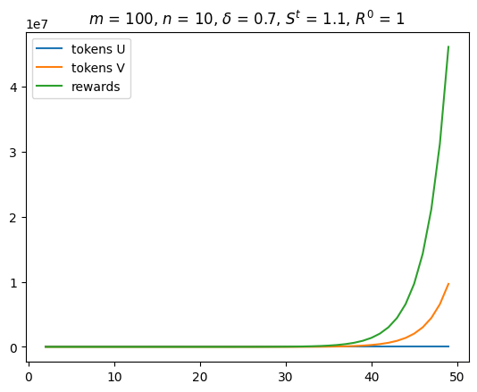
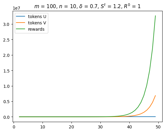
Figure 4: The effect of risk free rate ($\delta$) on rewards growth when no buy back condition: a smaller $\delta$ might trigger an exponential increase in both rewards and validators staked amounts (compare the right picture with the corresponding in Figure 2).

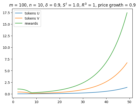
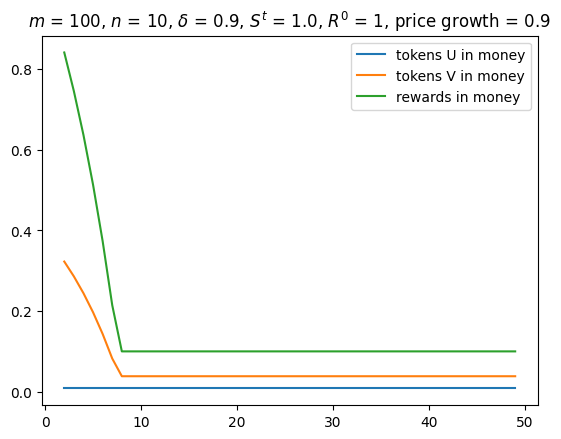
Figure 5: The effect of non-stable prices on rewards and validators staked tokens. We set decreasing prices according to the price growth parameter $\delta\mathcal{R}=0.9$. Though the rewards and staked tokens increase exponentially (left) their value expressed in money – rewards and staked tokens market cap – does not (right).

3.4 Policy that accommodates and implements the stable price equilibrium

In this section, we consider the fundamental question of how one can compute and implement an equilibrium with stable prices satisfying the no buy back condition. Stable prices require to keep a precise amount of tokens of users (on one side) and of tokens of validators (on the other side) given by Corollary 1. The no buy back condition requires the system to set the rewards so to satisfy the condition in Theorem 2. For the sake of exposition, we next describe an implementation for the reward and service fee schemes in (16).

Given parameters and constraints.

1. The risk free rate $r$ and thus the discount factor $\delta=1/(1+r)$.

2. The total number $m$ of users and the total number $n$ of validators (both constant over time).

3. There is no need for the system to buy back tokens (Definition 3).

System parameters.

The system design depends on essentially two parameters:

1. Total amount of service $S^{(t)}$ which is divided among the users at each step $t$.

2. Total amount of rewards $R^{(t)}$ which is distributed to the validators at each step $t$.

Assumption.

By the beginning of Subround II (buy or sell) of a current round $t$, each user knows the next total amount of service $S^{(t+1)}$ available in the next round, and each validator knows the total rewards $R^{(t+1)}$ available in the next round.

Suggested equilibrium description and properties.

At each round $t\geq 0$,

1. Users strategies:

   1. Start with $\mathbb{TK}_{U}^{(t)}=\frac{S^{(t)}}{m}\cdot\delta\cdot\kappa_{S}$ tokens, where $\kappa_{S}=g(n)\cdot\frac{m-1}{m}\cdot s^{\prime}(1/m)$.

   2. Spend all these tokens to get $S^{(t)}\cdot s(1/m)$ units of service.

   3. Given the service level $S^{(t+1)}$ of next round, buy $b_{U}^{(t)}=\mathbb{TK}_{U}^{(t+1)}$ tokens required for the next round according to Item 1a.

2. Validators strategies:

   1. Start with $\mathbb{TK}_{V}^{(t)}=\frac{R^{(t)}}{n}\cdot\frac{\delta}{1-\delta}\cdot\kappa_{R}$ tokens, where $\kappa_{R}=\frac{n-1}{n}\cdot r^{\prime}(1/n)$.

   2. Stake all these tokens to get $R^{(t)}\cdot r(1/n)$ new tokens as reward.

   3. Given the rewards $R^{(t+1)}$ of next round, sell this amount of tokens (if negative, buy tokens):

      $$s_{V}^{(t)}=\left(R^{(t)}-R^{(t+1)}\right)\cdot\frac{\delta}{1-\delta}\cdot\kappa_{R}+R^{(t)}\cdot r(1/n)$$ (31)

      which yields the required $\mathbb{TK}_{V}^{(t+1)}$ tokens for next round $t+1$ according to Item 2a.

3. System actions:

   1. Set the next service level $S^{(t+1)}$ and the next total rewards $R^{(t+1)}$ so that

      $$m\cdot S^{(t+1)}\cdot\delta\cdot\kappa_{S}\geq n\cdot\left(R^{(t)}-R^{(t+1)}\right)\cdot\frac{\delta}{1-\delta}\cdot\kappa_{R}+n\cdot R^{(t)}\cdot r(1/n)$$ (32)

      which guarantees the no buy back condition, that is, $m\cdot b_{U}^{(t)}\geq n\cdot s_{V}^{(t)}$.

   2. Announce the next service level $S^{(t+1)}$ and the next rewards $R^{(t+1)}$ before the token buy or sell (Subround II) begins.

   3. Sell the required amount of tokens, $m\mathbb{TK}_{U}^{(t+1)}-ns_{V}^{(t)}$, to match demand during Subround II.

4. Prices: all tokens are exchanged at a stable price $\mathbb{PRICE}^{(t)}=1$.

4 A two-token model

In this section, we consider a natural variant of the previous (single-token) model to the case in which we have two tokens, token $\mathbf{A}$ and $\mathbf{B}$, whose use and purpose is as follows:

• token $\mathbf{B}$ is used by the users to pay and get the service, and

• token $\mathbf{A}$ is used by the validators for staking to get rewarded with more tokens (of both types).

A number of existing systems follow a similar two-token scheme (see Figure 6 for some examples) and a model based on the similar assumptions has been recently given by Dimitri (2023). Both tokens can be exchanged in the spot market as before, and thus we have a price for each token (see Figure 7 for some additional notation for the two-token model). The corresponding utilities are naturally given by

$$U_{i}^{(\delta,\infty)}=\sum_{t=0}^{\infty}\delta^{t}\cdot U_{i}^{(t)}\ , U_{i}^{(t)}= S_{i}^{(t)}\cdot g(n)-{b_{i}}_{\mathbf{A}}^{(t)}\cdot{\mathbb{PRICE}}_{\mathbf{A}}^{(t)}-{b_{i}}_{\mathbf{B}}^{(t)}\cdot{\mathbb{PRICE}}_{\mathbf{B}}^{(t)}\ .$$ (33)

$$V_{j}^{(\delta,\infty)}=\sum_{t=0}^{\infty}\delta^{t}\cdot V_{j}^{(t)}\ , V_{j}^{(t)}= {s_{j}}_{\mathbf{A}}^{(t)}\cdot{\mathbb{PRICE}}_{\mathbf{A}}^{(t)}+{s_{j}}_{\mathbf{B}}^{(t)}\cdot{\mathbb{PRICE}}_{\mathbf{B}}^{(t)}-v\ .$$ (34)

System	token $\mathbf{A}$	purpose	token $\mathbf{B}$	purpose	reference
DFINITY	ICP	staking & rewards	Cycle	computation (service)	(Team, 2022)
NEO	NEO	staking	GAS	pay transactions	(neo.org, )
Axie Infinity	AXS	governance and staking	SLP	play (breeding Axie)	(Axi, 2021)

Figure 6: Examples of two-token systems.

• $R^{(t)}=({R}_{\mathbf{A}}^{(t)},{R}_{\mathbf{B}}^{(t)})$ is the reward at time $t$ • $s^{(t)}_{j}=({s_{j}}_{\mathbf{A}}^{(t)},{s_{j}}_{\mathbf{B}}^{(t)})$ is the selling strategy of validator $j$ • $b^{(t)}_{i}=({b_{i}}_{\mathbf{A}}^{(t)},{b_{i}}_{\mathbf{B}}^{(t)})$ is the buying strategy of user $i$ • $u_{i}^{(t)}$ is the amount of token $\mathbf{A}$ used by user $i$ to pay for the service • $\mathbb{TK}_{p}^{(t)}=(\mathbf{A}_{p}^{(t)},\mathbf{B}_{p}^{(t)})$ are the token holdings of a generic player $p$ (a user or a validator) • $\mathbb{PRICE}^{(t)}=({\mathbb{PRICE}}_{\mathbf{A}}^{(t)},{\mathbb{PRICE}}_{\mathbf{B}}^{(t)})$ are the prices of the two tokens

Figure 7: Notation for the two-token model.

For the sake of exposition, we consider the simpler reward sharing and payment schemes (14) in Häfner (2023), where token $\mathbf{A}$ is used for staking, and each validator $j$ is rewarded with quantities $R_{\mathbf{A}j}^{(t)}$ and $R_{\mathbf{B}j}^{(t)}$ of tokens $\mathbf{A}$ and $\mathbf{B}$, respectively. Users service level depends on the amount of token $\mathbf{B}$ they use. Thus, we have

$$S_{i}^{(t)}=S^{(t)}\cdot\left(\frac{u_{i}^{(t)}}{\sum_{k}u_{k}^{(t)}}\right)\ , R_{\mathbf{A}j}^{(t)}={R}_{\mathbf{A}}^{(t)}\cdot\left(\frac{\mathbf{A}_{j}^{(t)}}{\sum_{v}\mathbf{A}_{v}^{(t)}}\right)\ , R_{\mathbf{B}j}^{(t)}={R}_{\mathbf{B}}^{(t)}\cdot\left(\frac{\mathbf{A}_{j}^{(t)}}{\sum_{v}\mathbf{A}_{v}^{(t)}}\right)\ .$$ (35)

The validators’ selling constraint for the single token (5) extends naturally into

$$\mathbf{A}_{j}^{(t+1)}=\mathbf{A}_{j}^{(t)}+R_{\mathbf{A}j}^{(t)}-{s_{j}}_{\mathbf{A}}^{(t)}\geq 0$$ (36)

$$\mathbf{B}_{j}^{(t+1)}=\mathbf{B}_{j}^{(t)}+R_{\mathbf{B}j}^{(t)}-{s_{j}}_{\mathbf{B}}^{(t)}\geq 0$$ (37)

Similarly, the users’ selling constraint for the single token (6) extends as follows:

$$\mathbf{A}_{i}^{(t+1)}=\mathbf{A}_{i}^{(t)}+{b_{i}}_{\mathbf{A}}\geq 0$$ (38)

$$\mathbf{B}_{i}^{(t+1)}=\mathbf{B}_{i}^{(t)}-u_{i}^{(t)}+{b_{i}}_{\mathbf{B}}\geq 0$$ (39)

where the asymmetry is due to the fact that only token $\mathbf{B}$ is used for getting the service, by paying $u_{i}^{(t)}$ tokens. We next generalize the condition of (symmetric) equilibrium (Definition 1 and Remark 1) by requiring a “minimal” set of selling constraints to be non-strict (see Remark 4 below).

Definition 4 (symmetric equilibrium two tokens).

Consider a system policy given by (35), and a triple of users’ strategies, validators’ strategies, and prices, $\{(u_{i}^{(t)},b_{i}^{(t)}),s_{j}^{(t)},\mathbb{PRICE}^{(t)}\}$, such that the corresponding selling constraints of users (38)-(39) and of validators (36)-(37) are satisfied. We say that such a triple is an equilibrium if, for every user $i$ and every validator $j$

1. $(u_{i}^{(t)},b_{i}^{(t)})$ maximizes the discounted utility (33) of user $i$, given all other strategies

2. $s_{j}^{(t)}$ maximizes the discounted utility (34) of validator $j$, given all other strategies

3. the selling constraint of token $\mathbf{B}$ are non-strict for user $i$ (resp., token $\mathbf{A}$ for validator $j$), and thus the corresponding token holdings are strictly positive, that is, $\mathbf{B}_{i}^{(t)}>0$ and $\mathbf{A}_{j}^{(t)}>0$

Moreover, we say that such an equilibrium is symmetric if the token holdings of all users are the same, and similarly, if all token holdings of all validators are the same. In particular, we have

$$\mathbf{B}_{i}^{(t)}=\mathbf{B}_{U}^{(t)}>0 \mathbf{A}_{j}^{(t)}=\mathbf{A}_{V}^{(t)}>0$$ (40)

for all users $i$ and for all validators $j$ and for all $t$.

Remark 4 (minimal strict selling constraints).

Note that in the definition above, each type of player – validator or user – has non-strict selling constraint only in its own “main purpose” token. This corresponds to the natural requirement of continuous participation in staking and in accessing and paying for the service. Furthermore, the price analysis below implies that equilibria with certain desired prices are impossible if some of the other selling constraints is also strict.

The proof of the next two lemmas is given in Section A.2. Next lemma is the generalization of Lemma 1 to two tokens, and it provides conditions in the prices based on the validators’ strategies.

Lemma 3 (validators part).

In the two-token model, the corresponding prices at any symmetric equilibrium must satisfy the following conditions. If the selling constraints of $\mathbf{B}$ are non-strict, then

$${\mathbb{PRICE}}_{\mathbf{B}}^{(t-1)} =\delta\cdot{\mathbb{PRICE}}_{\mathbf{B}}^{(t)}\ .$$ (41)

If the selling constraints of $\mathbf{A}$ are non-strict, then

$${\mathbb{PRICE}}_{\mathbf{A}}^{(t-1)} =\delta\cdot{\mathbb{PRICE}}_{\mathbf{A}}^{(t)}\cdot(1+{\mathcal{I}}_{\mathbf{A}}^{(t)})+\delta\cdot{\mathbb{PRICE}}_{\mathbf{B}}^{(t)}\cdot{\mathcal{I}}_{\mathbf{B}}^{(t)}\ ,$$ (42)

where

$${\mathcal{I}}_{\mathbf{A}}^{(t)}:=\frac{{R}_{\mathbf{A}}^{(t)}}{n\mathbf{A}^{(t)}_{V}}\frac{n-1}{n}\ , {\mathcal{I}}_{\mathbf{B}}^{(t)}:=\frac{{R}_{\mathbf{B}}^{(t)}}{n\mathbf{A}^{(t)}_{V}}\frac{n-1}{n}\ .$$ (43)

and $\mathbf{A}_{V}^{(t)}$ is the token holding (staking) of any validator at this equilibrium.

Note that in absence of token $\mathbf{B}$, we recover the result in Lemma 1 for a single token. In this case, only token $\mathbf{A}$ is used for staking and for rewards, and thus ${R}_{\mathbf{B}}^{(t)}=0={\mathcal{I}}_{\mathbf{B}}^{(t)}$. The two quantities in $\eqref{eq:two-token-inflations}$ have an intuitive meaning as they correspond to the total amount of tokens rewarded – in each of the two tokens – over the total amount of staked tokens – the latter comprise only tokens $\mathbf{A}$. Note that these two expressions in $\eqref{eq:two-token-inflations}$ are not symmetric in the two tokens, as the staking token $\mathbf{A}$ appears in both denominators.

We next consider how the users’ buying strategies relate to the prices.

Lemma 4 (users part).

In the two-token model, the corresponding prices at any symmetric equilibrium must satisfy the following conditions. If the buying constraints of $\mathbf{B}$ are non-strict, then

$${\mathbb{PRICE}}_{\mathbf{B}}^{(t-1)}=\delta\cdot\begin{cases}\mathcal{S}^{(t)}&\text{if }u_{i}^{(t)}=\mathbf{B}_{U}^{(t)}\\ {\mathbb{PRICE}}_{\mathbf{B}}^{(t)}&\text{if }u_{i}^{(t)}<\mathbf{B}_{U}^{(t)}\end{cases} \mathcal{S}^{(t)}=\frac{S^{(t)}}{m\mathbf{B}_{U}^{(t)}}\cdot g(n)\cdot\frac{m-1}{m}$$ (44)

Moreover, if the buying constraints of $\mathbf{A}$ are non-strict, then

$${\mathbb{PRICE}}_{\mathbf{A}}^{(t-1)} =\delta\cdot{\mathbb{PRICE}}_{\mathbf{A}}^{(t)}$$ (45)

4.1 Generic symmetric equilibria

The following class of generic equilibria captures equilibria in the two-token model where prices of token $\mathbf{B}$ satisfy (20), thus in particular the case in which we aim at stable prices for token $\mathbf{B}$ used by the user to get the service.

Definition 5 (generic symmetric equilibrium for two tokens).

A symmetric equilibrium for the two token model is generic if the following conditions hold for all $t\geq 1$:

1. The service to fees ratio is constant,

   $$Ser2Fees_{\mathbf{B}}^{(t)}:=\frac{S^{(t)}}{m\mathbf{B}_{U}^{(t)}\cdot{\mathbb{PRICE}}_{\mathbf{B}}^{(t)}}=Ser2Fees_{\mathbf{B}}\ .$$ (46)

2. The prices of $\mathbf{B}$ satisfy

   $${\mathbb{PRICE}}_{\mathbf{B}}^{(t-1)}= \delta\cdot{\mathbb{PRICE}}_{\mathbf{B}}^{(t)}\cdot Ser2Fees_{\mathbf{B}}\cdot\kappa_{S}$$ (47)

   where constant $\kappa_{S}$ depends only on the number of users $m$, the number of validators $n$, and on the service fee scheme.

3. Each user $i$ starts round $t$ with the same token holding $\mathbf{B}_{U}^{(t)}$, uses all its current holding tokens for the service ($u_{i}^{(t)}=\mathbf{B}_{U}^{(t)}$), and buys new tokens needed for the next round accordingly ($b_{i}^{(t)}=\mathbf{B}_{U}^{(t+1)}$).

4. For the following rewards to stake ratios,

   $$Rew_{\mathbf{A}}2Stake^{(t)}:=\frac{{R}_{\mathbf{A}}^{(t)}}{n\mathbf{A}_{V}^{(t)}} Rew_{\mathbf{B}}2Stake^{(t)}:=\frac{{R}_{\mathbf{B}}^{(t)}}{n\mathbf{A}_{V}^{(t)}}$$ (48)

   the prices of $\mathbf{A}$ satisfy

   $${\mathbb{PRICE}}_{\mathbf{A}}^{(t-1)} =\delta\cdot{\mathbb{PRICE}}_{\mathbf{A}}^{(t)}\cdot(1+Rew_{\mathbf{A}}2Stake^{(t)}\cdot\kappa_{R})+\delta\cdot{\mathbb{PRICE}}_{\mathbf{B}}^{(t)}\cdot Rew_{\mathbf{B}}2Stake^{(t)}\cdot\kappa_{R}\ ,$$ (49)

   where constant $\kappa_{R}$ depends only on the number of users $n$, and on the rewards sharing scheme.

Theorem 3.

Any symmetric equilibrium for the two-token model with the reward and service fee schemes in (35) and whose prices of token $\mathbf{B}$ satisfy (20) is a generic symmetric equilibrium. This in particular holds true for the case of stable prices for token $\mathbf{B}$.

4.2 No buy back in the two-token model

In this section, we study the implications of no buy back in the two-token model. As for the single token setting, we aim at equilibria where the system does not need to buy back tokens of either type.

Definition 6 (no buy back two tokens).

We say that a symmetric equilibrium in the two-token model satisfies the no buy back condition if no additional tokens (of either type) are bought at any round by the system, that is, $m{b_{i}}_{\mathbf{B}}^{(t)}\geq n{s_{j}}_{\mathbf{B}}^{(t)}$ and $m{b_{i}}_{\mathbf{A}}^{(t)}\geq n{s_{j}}_{\mathbf{A}}^{(t)}$.

Theorem 4.

In any generic symmetric equilibrium, there is a maximum monetary reward for validators in terms of tokens $\mathbf{B}$ that can be awarded without violating the no buy back condition. In particular, it must hold

$${R}_{\mathbf{B}}^{(t)}\cdot{\mathbb{PRICE}}_{\mathbf{B}}^{(t)}\leq\delta\cdot S^{(t+1)}\cdot\frac{\kappa_{S}}{n\cdot r(1/n)}\ .$$ (50)

This is because validators always sell all the newly rewarded $\mathbf{B}$ tokens and users buy (only) tokens of type $\mathbf{B}$, thus implying that validators keep all their tokens $\mathbf{A}$ and possibly buy new ones, $\mathbf{A}_{V}^{(t)}\geq\mathbf{A}_{V}^{(t-1)}$.

Proof.

We consider the two inequalities of the no buy back condition (Definition 6) separately.

1. For tokens of type $\mathbf{B}$, we observe that, for ${\mathbb{PRICE}}_{\mathbf{B}}^{(t-1)}\neq\delta\cdot{\mathbb{PRICE}}_{\mathbf{B}}^{(t)}$, the users buying strategies satisfy

   $$m{b_{i}}_{\mathbf{B}}^{(t)}=m\mathbf{B}_{U}^{(t+1)}=\frac{S^{(t+1)}}{Ser2Fees_{\mathbf{B}}^{(t+1)}\cdot{\mathbb{PRICE}}_{\mathbf{B}}^{(t+1)}}=S^{(t+1)}\cdot\frac{\delta}{{\mathbb{PRICE}}_{\mathbf{B}}^{(t)}}\cdot\kappa_{S}\ .$$ (51)

   Moreover, the validators’ selling strategies satisfy

   $${s_{j}}_{\mathbf{B}}^{(t)}={R}_{\mathbf{B}}^{(t)}\cdot r(1/n)\ ,$$ (52)

   since the validators selling constraint for tokens of type $\mathbf{B}$ must be strict, and thus $\mathbf{B}_{i}^{(t)}=0$ for all $t$. Therefore the no buy back condition for tokens of type $\mathbf{B}$ is equivalent to

   $$n\cdot{R}_{\mathbf{B}}^{(t)}\cdot r(1/n)\leq S^{(t+1)}\cdot\frac{\delta}{{\mathbb{PRICE}}_{\mathbf{B}}^{(t)}}\cdot\kappa_{S}\ .$$ (53)

2. We also require no buy back for the tokens of type $\mathbf{A}$, which means that ${s_{j}}_{\mathbf{A}}^{(t)}=0$ because users never hold (and thus never buy) tokens of type $\mathbf{A}$. Hence, $\mathbf{A}_{V}^{(t+1)}=\mathbf{A}_{V}^{(t)}+{R}_{\mathbf{A}}^{(t)}\cdot r(1/n)+{b_{j}}_{\mathbf{A}}^{(t)}$ with ${b_{j}}_{\mathbf{A}}^{(t)}\geq 0$.

This completes the proof. ∎

4.3 Stable price mechanism in two-token model

We next‘ describe a simple mechanism which implements stable prices for token $\mathbf{B}$, while the price of $\mathbf{A}$ is strictly decreasing:

1. In order to have stable prices for $\mathbf{B}$ and no buy back, we set ${R}_{\mathbf{B}}^{(t)}$ such that

   $${R}_{\mathbf{B}}^{(t)}\cdot{\mathbb{PRICE}}_{\mathbf{B}}^{(t)}=S^{(t+1)}\cdot L$$ (54)

   where $L$ is the constant given by Theorem 4 that makes the no buy back condition hold tightly. Furthermore, we set ${R}_{\mathbf{A}}^{(t)}=0$.

2. The buying strategies for token $\mathbf{A}$ are “no buy and no sell”, that is, $\mathbf{A}_{V}^{(t)}=\mathbf{A}_{V}^{(0)}$, for a suitable $\mathbf{A}_{V}^{(0)}$ specified below. From the equation of the prices (42), we obtain

   $${\mathbb{PRICE}}_{\mathbf{A}}^{(t-1)} =\delta\cdot{\mathbb{PRICE}}_{\mathbf{A}}^{(t)}\cdot(1+{\mathcal{I}}_{\mathbf{A}}^{(t)})+\delta\cdot{\mathbb{PRICE}}_{\mathbf{B}}^{(t)}\cdot{\mathcal{I}}_{\mathbf{B}}^{(t)}$$ (55)

   $$=\delta\cdot{\mathbb{PRICE}}_{\mathbf{A}}^{(t)}+\delta\cdot{\mathbb{PRICE}}_{\mathbf{B}}^{(t)}\cdot\frac{{R}_{\mathbf{B}}^{(t)}}{n\mathbf{A}^{(t)}_{V}}\frac{n-1}{n}$$ (56)

   $$=\delta\cdot{\mathbb{PRICE}}_{\mathbf{A}}^{(t)}+\delta\cdot S^{(t+1)}\cdot L\cdot\frac{1}{n\mathbf{A}_{V}^{(0)}}\frac{n-1}{n}$$ (57)

   and by rearranging the terms we get

   $${\mathbb{PRICE}}_{\mathbf{A}}^{(t)} =\frac{{\mathbb{PRICE}}_{\mathbf{A}}^{(t-1)}}{\delta}-S^{(t+1)}\cdot\frac{L}{\mathbf{A}_{V}^{(0)}}\frac{n-1}{n^{2}}\ ,$$ (58)

   which implies

   $${\mathbb{PRICE}}_{\mathbf{A}}^{(t)} <\frac{{\mathbb{PRICE}}_{\mathbf{A}}^{(0)}}{\delta^{t}}\ .$$ (59)

3. From the previous equation, the discounted utility of validators, if deviating by selling all tokens $\mathbf{A}$ at some step $\tau$, is at most

   $$\delta^{\tau}\cdot\mathbf{A}_{V}^{(0)}\cdot{\mathbb{PRICE}}_{\mathbf{A}}^{(\tau)}<\mathbf{A}_{V}^{(0)}\cdot{\mathbb{PRICE}}_{\mathbf{A}}^{(0)}$$ (60)

   while the discounted utility for the suggested strategies (equilibrium) equals

   $$\sum_{t=0}^{\infty}\delta^{t}\cdot({R}_{\mathbf{B}}^{(t)}\cdot{\mathbb{PRICE}}_{\mathbf{B}}^{(t)}-v)=\sum_{t=0}^{\infty}\delta^{t}\cdot(S^{(t+1)}\cdot L)-\frac{v}{1-\delta}\ .$$ (61)

4. In order to have feasible (nonnegative) prices, we need to set the initial payments and token holdings sufficiently high.

Theorem 5.

For any service level satisfying Assumption 1 and any reward and service sharing schemes satisfying Assumption 2, the strategies above are a symmetric equilibrium with stable prices for token $\mathbf{B}$ used by users for getting the service.

Proof.

We follow the same argument in (Häfner, 2023, Remark 2 (exhistence)) based on the following three conditions. First, the discounted utilities of all players (users and validators) assume finite values (as their instantaneous utilities are proportional to $S^{(t)}$). Second, these strategies are in some bounded interval $[\underline{\theta},\overline{\theta}]$. For the users this is obvious since they buy tokens proportionally to $S^{(t+1)}$. For the validators, they sell all ${R}_{\mathbf{B}}^{(t)}=O(S^{(t)})$ tokens $\mathbf{B}$, they never sell or buy tokens $\mathbf{A}$. Third, the utilities of the players are concave due to Assumption 2. ∎

4.3.1 Stable price mechanism implementation

At each round $t$, the system can infer infer $S^{(t+1)}$ from the total amount of tokens and the current price from (46). Moreover:

1. Users use (spend) $\mathbf{B}$ tokens proportionally to $S^{(t)}$ and buy new $\mathbf{B}$ tokens proportionally to $S^{(t+1)}$.

2. Validators’ rewards consist of only tokens $\mathbf{B}$ proportionally to the next round service level $S^{(t+1)}$.

3. Validators sell all these $\mathbf{B}$ that they get as rewards, and keep all $\mathbf{A}$ tokens they had from the beginning.

5 Conclusions and open questions

We investigate how the long-term equilibria between users, validators and token flows are different for blockchains with a single token (used for transaction fees and staking) and two separate tokens. While there are similarities, the two-token model affords additional flexibility that can handle a broader variation of service levels at equilibrium, with the added complexity of robustly keeping track of certain additional blockchain metrics. Specifically, to facilitate the implementation, a suitable proxy for the service level $S^{(t)}$ is essential. Using the fees as a proxy provides a good starting point, but additional work is needed to ensure that incentive compatibility from users and validators is maintained. In addition, it is possible that an oracle could provide additional valuable information, that does not necessarily exist on-chain (such as the volatility of the crypto markets). Would this substantially expand our design space and allow finer robust control, requiring only infrequent human intervention?

Appendix A Postponed Proofs

A.1 Proofs of Section 3

A.1.1 Proof of Lemma 2

In the following, we consider a generic symmetric equilibrium (Definition 1),

$$(u_{i}^{(t)},b_{i}^{(t)})=(u_{U}^{(t)},b_{U}^{(t)}) s_{j}^{(t)}=s_{V}^{(t)} \mathbb{PRICE}^{(t)}$$ (62)

for every user $i$ and every validator $j$, where the above strategies give the corresponding token holdings via (7). The proof follows the same steps as in (Häfner, 2023, Proof of Lemma 1).

1. Validators’ part. Denote by $\mathcal{V}_{j}^{t}$ the discounted utility of validator $j$ at equilibrium starting from step $t$. By the Principle of Optimality,

   $$\mathcal{V}_{j}^{t}=\max_{s_{j}^{(t)}}[\mathbb{PRICE}^{(t)}\cdot s_{j}^{(t)}-v]+\delta\mathcal{V}_{j}^{t+1}$$ (63)

   subject to the selling constraint (5). We next show that we must have

   $$\frac{\partial\mathcal{V}_{j}^{t}}{\partial s_{j}^{(t)}}=0 \Longrightarrow \mathbb{PRICE}^{(t)}=\delta\frac{\partial\mathcal{V}_{j}^{t+1}}{\partial\mathbb{TK}_{j}^{(t+1)}}$$ (64)

   The LHS uses (crucially) that in the equilibrium (Definition 1 and Remark 1) the selling constraint (5) is not binding (not strict), thus implying that the derivative must be zero at equilibrium. The RHS holds because

   $$\frac{\partial\mathcal{V}_{j}^{t}}{\partial s_{j}^{(t)}}=\mathbb{PRICE}^{(t)}+\delta\frac{\partial\mathcal{V}_{j}^{t+1}}{\partial s_{j}^{(t)}} \frac{\partial\mathcal{V}_{j}^{t+1}}{\partial s_{j}^{(t)}}=\frac{\partial\mathbb{TK}_{j}^{(t+1)}}{\partial s_{j}^{(t)}}\frac{\partial\mathcal{V}_{j}^{t+1}}{\partial\mathbb{TK}_{j}^{(t+1)}}\stackrel{{\scriptstyle\eqref{eq:token-holdings}}}{{=}}(-1)\frac{\partial\mathcal{V}_{j}^{t+1}}{\partial\mathbb{TK}_{j}^{(t+1)}}$$ and (65)

   Next observe that, since $s_{j}^{(t)}=\mathbb{TK}_{j}^{(t)}+R_{j}^{(t)}-\mathbb{TK}_{j}^{(t+1)}$, we also have

   $$\frac{\partial\mathcal{V}_{j}^{t}}{\partial\mathbb{TK}_{j}^{(t)}}=\mathbb{PRICE}^{(t)}\cdot\left(1+R^{(t)}\cdot\frac{(n-1)\mathbb{TK}_{V}^{(t)}}{(\mathbb{TK}_{j}^{(t)}+(n-1)\mathbb{TK}_{V}^{(t)})^{2}}\cdot r^{\prime}\left(\frac{\mathbb{TK}_{j}^{(t)}}{\mathbb{TK}_{j}^{(t)}+(n-1)\mathbb{TK}_{V}^{(t)}}\right)\right)$$ (66)

   Plugging this into (64), we obtain

   $$\mathbb{PRICE}^{(t-1)}=\delta\cdot\mathbb{PRICE}^{(t)}\cdot\left(1+\frac{R^{(t)}}{\mathbb{TK}_{V}^{(t)}}\cdot\frac{n-1}{n^{2}}\cdot r^{\prime}(\frac{1}{n})\right)$$ (67)

2. Users’ part. Denote by $\mathcal{U}_{i}^{t}$ the discounted utility of user $i$ at equilibrium starting from step $t$, By the Principle of Optimality,

   $$\mathcal{U}_{i}^{t}=\max_{(u_{i}^{(t)},b_{i}^{(t)})}[S^{(t)}\cdot g(n)\cdot s(u_{i}^{(t)},u_{-i}^{(t)})-\mathbb{PRICE}^{(t)}\cdot b_{i}^{(t)}]+\delta\mathcal{U}_{i}^{t+1}$$ (68)

   where $(u_{i}^{(t)},b_{i}^{(t)})$ satisfies the corresponding buying constraint (6), and $u_{-i}^{(t)}$ denotes the use strategies of all other users. We next show that we must have

   $$\frac{\partial\mathcal{U}_{i}^{t}}{\partial b_{i}^{(t)}}=0 \Longrightarrow \mathbb{PRICE}^{(t)}=\delta\frac{\partial\mathcal{U}_{i}^{t+1}}{\partial\mathbb{TK}_{i}^{(t+1)}}$$ (69)

   The LHS uses (crucially) that in the equilibrium (Definition 1 and Remark 1) the buying constraint (6) is not binding (not strict), thus implying that the derivative must be zero at equilibrium. The RHS holds because

   $$\frac{\partial\mathcal{U}_{i}^{t}}{\partial b_{i}^{(t)}}=-\mathbb{PRICE}^{(t)}+\delta\frac{\partial\mathcal{U}_{i}^{t+1}}{\partial b_{i}^{(t)}} \frac{\partial\mathcal{U}_{i}^{t+1}}{\partial b_{i}^{(t)}}=\frac{\partial\mathbb{TK}_{i}^{(t+1)}}{\partial b_{i}^{(t)}}\frac{\partial\mathcal{U}_{i}^{t+1}}{\partial\mathbb{TK}_{i}^{(t+1)}}\stackrel{{\scriptstyle\eqref{eq:token-holdings}}}{{=}}(+1)\frac{\partial\mathcal{U}_{i}^{t+1}}{\partial\mathbb{TK}_{i}^{(t+1)}}$$ and (70)

   We next show that

   $$\frac{\partial\mathcal{U}_{i}^{t}}{\partial\mathbb{TK}_{i}^{(t)}}=\begin{cases}S^{(t)}\cdot g(n)\cdot\frac{(m-1)\mathbb{TK}_{U}^{(t)}}{(\mathbb{TK}_{i}^{t}+(m-1)\mathbb{TK}_{U}^{(t)})^{2}}\cdot s^{\prime}(\frac{\mathbb{TK}_{i}^{t}}{\mathbb{TK}_{i}^{t}+(m-1)\mathbb{TK}_{U}^{(t)}})&\text{if at equilibrium }u_{i}^{(t)}=\mathbb{TK}_{U}^{(t)}\\ \mathbb{PRICE}^{(t)}&\text{if at equilibrium }u_{i}^{(t)}<\mathbb{TK}_{U}^{(t)}\end{cases}$$ (71)

   thus implying

   $$\mathbb{PRICE}^{(t-1)}=\delta\cdot\begin{cases}\frac{S^{(t)}}{\mathbb{TK}_{U}^{(t)}}\cdot g(n)\cdot\frac{m-1}{m^{2}}\cdot s^{\prime}(\frac{1}{m})&\text{if at equilibrium }u_{i}^{(t)}=\mathbb{TK}_{U}^{(t)}\\ \mathbb{PRICE}^{(t)}&\text{if at equilibrium }u_{i}^{(t)}<\mathbb{TK}_{U}^{(t)}\end{cases}$$ (72)

   We distinguish the two cases in (71). If at equilibrium $u_{i}^{(t)}=\mathbb{TK}_{U}^{(t)}$, then $b_{i}^{(t)}=\mathbb{TK}_{i}^{(t+1)}$ and

   $$\mathcal{U}_{i}^{t}=[S^{(t)}\cdot g(n)\cdot s(\mathbb{TK}_{i}^{(t)},\mathbb{TK}_{-iU}^{(t)})-\mathbb{PRICE}^{(t)}\cdot\mathbb{TK}_{i}^{(t+1)}]+\delta\mathcal{U}_{i}^{t+1}$$ (73)

   where $\mathbb{TK}_{-iU}^{(t)}$ denotes the token holdings at equilibrium of all but user $i$ at step $t$. The above equation implies that the corresponding derivative satisfies

   $$\frac{\partial\mathcal{U}_{i}^{t}}{\partial\mathbb{TK}_{i}^{(t)}}=S^{(t)}\cdot g(n)\cdot\frac{m-1}{m^{2}}\cdot s^{\prime}(\frac{1}{m})$$ (74)

   If at equilibrium $u_{i}^{(t)}<\mathbb{TK}_{U}^{(t)}$, then $b_{i}^{(t)}=\mathbb{TK}_{i}^{(t+1)}-\mathbb{TK}_{i}^{(t)}+u_{i}^{(t)}$ and

   $$\mathcal{U}_{i}^{t}=[S^{(t)}\cdot g(n)\cdot s(u_{i}^{(t)},u_{-iU}^{(t)})-\mathbb{PRICE}^{(t)}\cdot b_{i}^{(t)}]+\delta\mathcal{U}_{i}^{t+1}$$ (75)

   thus implying that the corresponding derivative satisfies

   $$\frac{\partial\mathcal{U}_{i}^{t}}{\partial\mathbb{TK}_{i}^{(t)}}=-\mathbb{PRICE}^{(t)}\cdot\frac{\partial b_{i}^{(t)}}{\partial\mathbb{TK}_{i}^{(t)}}=-\mathbb{PRICE}^{(t)}\cdot(-1)=\mathbb{PRICE}^{(t)}$$ (76)

   as in this case the optimal $u_{i}^{(t)}<\mathbb{TK}_{U}^{(t)}=\mathbb{TK}_{i}^{(t)}$ is not affected by $\mathbb{TK}_{i}^{(t)}$.

A.1.2 Proof of Theorem 1

Condition (20) on the prices and Lemma 2 imply $\delta\mathcal{R}^{(t)}=\gamma$. The result follows from the definition of $\mathcal{R}^{(t)}$ and $\mathcal{S}^{(t)}$ and from identity (19) from Lemma 2 (second part).

A.2 Proofs of Section 4

A.2.1 Proof of Lemma 3

By adapting the analysis in Häfner (2023), the discounted utility at equilibrium of validator $j$ starting from step $t$ satisfies

$$\mathcal{V}_{j}^{(t)}=\max_{s_{j}^{(t)}}[{\mathbb{PRICE}}_{\mathbf{A}}^{(t)}\cdot{s_{j}}_{\mathbf{A}}^{(t)}+{\mathbb{PRICE}}_{\mathbf{B}}^{(t)}\cdot{s_{j}}_{\mathbf{B}}^{(t)}-v]+\delta\mathcal{V}_{j}^{(t+1)}$$ (77)

where in a symmetric equilibrium the selling constraints (36) and (37) for validator $j$ become

$$\mathbf{A}_{j}^{(t+1)}=\mathbf{A}_{j}^{(t)}+{R}_{\mathbf{A}}^{(t)}\frac{\mathbf{A}_{j}^{(t)}}{\mathbf{A}_{j}^{(t)}+(n-1)\mathbf{A}_{V}^{(t)}}-{s_{j}}_{\mathbf{A}}^{(t)}\geq 0$$ (78)

$$\mathbf{B}_{j}^{(t+1)}=\mathbf{B}_{j}^{(t)}+{R}_{\mathbf{B}}^{(t)}\frac{\mathbf{A}_{j}^{(t)}}{\mathbf{A}_{j}^{(t)}+(n-1)\mathbf{A}_{V}^{(t)}}-{s_{j}}_{\mathbf{B}}^{(t)}\geq 0$$ (79)

(Note that the two expressions above are not symmetric as token $\mathbf{A}$ is the only one used for staking – the fraction term is identical.) We next show that, under the optimal selling policy at equilibrium $s_{j}^{(t)}$ we must have

$$\frac{\partial\mathcal{V}_{j}^{(t)}}{\partial{s_{j}}_{\mathbf{A}}^{(t)}}=0 \Longleftrightarrow {\mathbb{PRICE}}_{\mathbf{A}}^{(t)}=\delta\frac{\partial\mathcal{V}_{j}^{(t+1)}}{\partial\mathbf{A}_{j}^{(t+1)}}$$ (80)

The LHS uses (crucially) that in the equilibrium (Definition 1 and Remark 1) the selling constraint (78) is not binding (not strict), thus implying that the derivative must be zero. The equivalence with the RHS is because

$$\frac{\partial\mathcal{V}_{j}^{(t)}}{\partial{s_{j}}_{\mathbf{A}}^{(t)}}={\mathbb{PRICE}}_{\mathbf{A}}^{(t)}+\delta\frac{\partial\mathcal{V}_{j}^{(t+1)}}{\partial{s_{j}}_{\mathbf{A}}^{(t)}} \frac{\partial\mathcal{V}_{j}^{(t+1)}}{\partial{s_{j}}_{\mathbf{A}}^{(t)}}=\frac{\partial\mathbf{A}_{j}^{(t+1)}}{\partial{s_{j}}_{\mathbf{A}}^{(t)}}\frac{\partial\mathcal{V}_{j}^{(t+1)}}{\partial\mathbf{A}_{j}^{(t+1)}}=(-1)\frac{\partial\mathcal{V}_{j}^{(t+1)}}{\partial\mathbf{A}_{j}^{(t+1)}}$$ and (81)

where $\frac{\partial\mathbf{A}_{j}^{(t+1)}}{\partial{s_{j}}_{\mathbf{A}}^{(t)}}=-1$ uses (again) that the selling constraint (78) is not binding (not strict). The exact same proof applies to the other token $\mathbf{B}$, using the corresponding selling constraint (79) to obtain

$$\frac{\partial\mathcal{V}_{j}^{(t)}}{\partial{s_{j}}_{\mathbf{B}}^{(t)}}=0 \Longleftrightarrow {\mathbb{PRICE}}_{\mathbf{B}}^{(t)}=\delta\frac{\partial\mathcal{V}_{j}^{(t+1)}}{\partial\mathbf{B}_{j}^{(t+1)}}$$ (82)

Next observe that

$$\mathcal{V}_{j}^{(t)}= {\mathbb{PRICE}}_{\mathbf{A}}^{(t)}{s_{j}}_{\mathbf{A}}^{(t)}+{\mathbb{PRICE}}_{\mathbf{B}}^{(t)}{s_{j}}_{\mathbf{B}}^{(t)}-v+\delta\mathcal{V}_{j}^{*t+1}$$ (83)

$$= {\mathbb{PRICE}}_{\mathbf{A}}^{(t)}\left[\mathbf{A}_{j}^{(t)}+{R}_{\mathbf{A}}^{(t)}\frac{\mathbf{A}_{j}^{(t)}}{\mathbf{A}_{j}^{(t)}+(n-1)\mathbf{A}_{V}^{(t)}}-\mathbf{A}_{j}^{(t+1)}\right]+$$ (84)

$${\mathbb{PRICE}}_{\mathbf{B}}^{(t)}\left[\mathbf{B}_{j}^{(t)}+{R}_{\mathbf{B}}^{(t)}\frac{\mathbf{A}_{j}^{(t)}}{\mathbf{A}_{j}^{(t)}+(n-1)\mathbf{A}_{V}^{(t)}}-\mathbf{B}_{j}^{(t+1)}\right]-v+\delta\mathcal{V}_{j}^{(t+1)}$$ (85)

thus implying

$$\frac{\partial\mathcal{V}_{j}^{(t)}}{\partial\mathbf{A}_{j}^{(t)}}= {\mathbb{PRICE}}_{\mathbf{A}}^{(t)}\left[1+{R}_{\mathbf{A}}^{(t)}\frac{(n-1)\mathbf{A}_{V}^{(t)}}{(\mathbf{A}_{j}^{(t)}+(n-1)\mathbf{A}_{V}^{(t)})^{2}}\right]+{\mathbb{PRICE}}_{\mathbf{B}}^{(t)}\left[{R}_{\mathbf{B}}^{(t)}\frac{(n-1)\mathbf{A}_{V}^{(t)}}{(\mathbf{A}_{j}^{(t)}+(n-1)\mathbf{A}_{V}^{(t)})^{2}}\right]$$ (86)

$$\frac{\partial\mathcal{V}_{j}^{(t)}}{\partial\mathbf{B}_{j}^{(t)}}= {\mathbb{PRICE}}_{\mathbf{B}}^{(t)}$$ (87)

Plugging these into (80) and (82), we obtain

$${\mathbb{PRICE}}_{\mathbf{A}}^{(t-1)}= \delta{\mathbb{PRICE}}_{\mathbf{A}}^{(t)}\left[1+\frac{{R}_{\mathbf{A}}^{(t)}}{\mathbf{A}^{(t)}_{V}}\frac{n-1}{n^{2}}\right]+\delta{\mathbb{PRICE}}_{\mathbf{B}}^{(t)}\left[\frac{{R}_{\mathbf{B}}^{(t)}}{\mathbf{A}_{V}^{(t)}}\frac{n-1}{n^{2}}\right]$$ (88)

$${\mathbb{PRICE}}_{\mathbf{B}}^{(t-1)}= \delta{\mathbb{PRICE}}_{\mathbf{B}}^{(t)}$$ (89)

which proves Lemma 3.

A.2.2 Proof of Lemma 4

The proof is identical to the one for the single token in Section A.1, users part. The equation for $\mathbf{B}$ comes from the same analysis of the single token. As for token $\mathbf{A}$, we observe that since token $\mathbf{A}$ does not affect the amount of service to $i$, we have $\frac{\partial\mathcal{U}_{i}^{(t)}}{\partial\mathbf{A}{{}_{i}}^{(t)}}={\mathbb{PRICE}}_{\mathbf{A}}^{(t)}$ for all $t$. The usual optimality conditions of strategy ${b_{i}}_{\mathbf{A}}$ also yields ${\mathbb{PRICE}}_{\mathbf{A}}^{(t)}=\delta\frac{\partial\mathcal{U}_{i}^{(t+1)}}{\partial{b_{j}}_{\mathbf{A}}^{(t)}}$. The latter quantity, by the previous equation with $t+1$ in place of $t$, equals $\delta{\mathbb{PRICE}}_{\mathbf{A}}^{(t+1)}$.

Appendix B An example of an alternative rewards scheme

Consider the following “soft cap” function based on the sigmoid (logistic) function $\sigma(x)=\frac{\mathrm{e}^{x}}{1+\mathrm{e}^{x}}$,

$$softcap(x,\tau,T):=1-\sigma(T\cdot(x-\tau))=\frac{1}{\mathrm{e}^{T\cdot(x-\tau)}+1}$$ (90)

Our reward function uses this soft cap, which intuitively aims at capping each validator’s stake to a fraction $1/n$ of the total stake:

$$r(x):=2x\cdot softcap(x,1/n,T)=\frac{2x}{\mathrm{e}^{T\cdot(x-\frac{1}{n})}+1}$$ (91)

In this case,

$$r^{\prime}(x)=-\dfrac{2\left(\left(Tx-1\right)\mathrm{e}^{T\cdot\left(x-\frac{1}{n}\right)}-1\right)}{\left(\mathrm{e}^{T\cdot\left(x-\frac{1}{n}\right)}+1\right)^{2}}\ , r^{\prime}(1/n)=1-T/2n\ .$$ (92)

Hence the condition $r^{\prime}(1/n)>0$ required in Assumption 2 is satisfied for all $n>T/2$, meaning that the designer can set $T$ in order to be satisfied for the number $n$ of validators.

References

• Axi (2021) Axie infinity whitepaper, 2021. URL https://whitepaper.axieinfinity.com/axs. NEO & GAS.
• Bakos and Halaburda (2019) Yannis Bakos and Hanna Halaburda. The role of cryptographic tokens and ICOs in fostering platform adoption. CESifo Working Paper, 2019. URL https://ideas.repec.org/p/ces/ceswps/_7752.html.
• Bakos and Halaburda (2022) Yannis Bakos and Hanna Halaburda. Overcoming the coordination problem in new marketplaces via cryptographic tokens. Information Systems Research, 33(4):1368–1385, 2022.
• Chitra (2021) Tarun Chitra. Competitive Equilibria Between Staking and On-chain Lending. Cryptoeconomic Systems, 0(1), 2021. https://cryptoeconomicsystems.pubpub.org/pub/chitra-staking-lending-equilibria.
• Cong et al. (2021) Lin William Cong, Ye Li, and Neng Wang. Tokenomics: Dynamic adoption and valuation. The Review of Financial Studies, 34(3):1105–1155, 2021.
• Cong et al. (2022) Lin William Cong, Ye Li, and Neng Wang. Token-based platform finance. Journal of Financial Economics, 144(3):972–991, 2022.
• Dimitri (2023) Nicola Dimitri. The economic value of dual-token blockchains. Mathematics, 11(17):3757, 2023. URL https://doi.org/10.3390/math11173757.
• Félez-Viñas et al. (2021) Ester Félez-Viñas, Sean Foley, Jonathan R Karlsen, and Jiri Svec. Better than bitcoin? can cryptocurrencies beat inflation? Available at SSNR, 2021. URL https://dx.doi.org/10.2139/ssrn.3970810.
• Häfner (2023) Samuel Häfner. Optimal decentralization and service provision on a blockchain platform with market frictions, September 2023. URL https://papers.ssrn.com/sol3/papers.cfm?abstract_id=3954773.
• Kiayias et al. (2023) Aggelos Kiayias, Philip Lazos, and Jan Christoph Schlegel. Would Friedman Burn your Tokens? arXiv preprint arXiv:2306.17025, 2023.
• Li and Mann (2018) Jiasun Li and William Mann. Digital tokens and platform building. 2018. URL http://dx.doi.org/10.2139/ssrn.3088726.
• (12) neo.org. URL https://neo.org/neogas#tokens. NEO & GAS.
• Pagnotta (2022) Emiliano S Pagnotta. Decentralizing money: Bitcoin prices and blockchain security. The Review of Financial Studies, 35(2):866–907, 2022.
• Prat et al. (2021) Julien Prat, Vincent Danos, and Stefania Marcassa. Fundamental Pricing of Utility Tokens. Working Papers hal-03096267, HAL, 2021. URL https://ideas.repec.org/p/hal/wpaper/hal-03096267.html.
• Schilling and Uhlig (2019) Linda Schilling and Harald Uhlig. Some simple bitcoin economics. Journal of Monetary Economics, 106:16–26, 2019.
• Sockin and Xiong (2023) Michael Sockin and Wei Xiong. A model of cryptocurrencies. Management Science, 69(11), 2023.
• Team (2022) The DFINITY Team. The internet computer for geeks. Cryptology ePrint Archive, Paper 2022/087, 2022. URL https://eprint.iacr.org/2022/087.