Can the NANOGrav observations constrain the geometry of the universe?

Abstract

The theory of inflation provides an elegant explanation for the nearly flat universe observed today, which represents one of the pillars of the standard cosmological model. However, recent studies have reported some deviations from a flat geometry, arguing that a closed universe would be instead favored by observations. Given its central role played in the cosmological context, this paper revisits the issue of spatial curvature in light of the stochastic gravitational wave background signal recently detected by the NANOGrav collaboration. For this purpose, we investigate the primordial gravitational waves generated during inflation and their propagation in the post-inflationary universe. We propose a new parametrization of the gravitational wave power spectrum, taking into account spatial curvature, the tensor-to-scalar ratio and the spectral index of tensor perturbations. Therefore, we compare the theoretical predictions with NANOGrav data to possibly constrain the geometry of the universe. We find that the choice of the priors has a significant effect on the computed posterior distributions. In particular, using flat uniform priors results in $\Omega_{\mathcal{K},0}=0.00\pm 0.67$ at the 68% confidence level. On the other hand, imposing a Planck prior, we obtain $\Omega_{\mathcal{K},0}=-0.05\pm 0.17$ at the 68% confidence level. This result aligns with the analysis of the cosmic microwave background radiation, and no deviations from a flat universe are found.

I Introduction

The inclusion of the cosmological constant ($\Lambda$) into Einstein’s equations of general relativity (GR) offers the simplest way to explain the current acceleration of the universe suggested by observations over the last two decades Carroll et al. (1992); Riess et al. (1998); Perlmutter et al. (1999); Peebles and Ratra (2003). The cosmic speed-up can be ascribed, more generally, to a mysterious fluid with negative pressure, known as dark energy, which propels the late-time dynamics Copeland et al. (2006); Frieman et al. (2008); Weinberg et al. (2013). Additionally, the total matter content in the universe is constituted of only a small fraction of baryons, while the main part is dominated by hypothetical dark matter particles that do not interact with the electromagnetic field Bond and Efstathiou (1984); Persic and Salucci (1992); D’Agostino et al. (2023a). On the other hand, the formation of cosmic structures arises from primordial quantum fluctuations that were stretched beyond the horizon during inflation Guth (1981). Subsequently, these fluctuations re-entered the horizon as density perturbations, giving rise to all the structures present in the universe Mukhanov et al. (1992). The inflationary mechanism is responsible for the nearly vanishing curvature, isotropy and homogeneity on large scales observed today Linde (1982). Overall, such a picture of the universe goes under the name of $\Lambda$-Cold Dark Matter $(\Lambda$CDM) scenario, which stands out as the standard model of cosmology Hinshaw et al. (2013); Aghanim et al. (2020).

Whilst the $\Lambda$CDM model has proven successful in explaining most observations theoretical limitations regarding the nature of the dark components cast doubt on its confirmation as the ultimate picture of the cosmos. Indeed, the debated origin of $\Lambda$, interpreted as the vacuum energy density, leads to the well-known fine-tuning problem Weinberg (1989); Padmanabhan (2003); D’Agostino et al. (2022). At the same time, recent tensions among cosmic data have questioned the validity of the standard paradigm to thoroughly describe the evolution of the universe Di Valentino et al. (2021); Riess et al. (2022); Perivolaropoulos and Skara (2022); D’Agostino and Nunes (2023). All this has motivated through the years the search for possible alternatives. Several examples, among the others, include dynamically evolving scalar fields Ratra and Peebles (1988); Caldwell et al. (1998); Tsujikawa (2013), unified dark models Kamenshchik et al. (2001); Scherrer (2004); Capozziello et al. (2018, 2019a); D’Agostino and Luongo (2022), or holographic dark energy Li (2004); D’Agostino (2019). Alternatively, it is possible to explain the universe’s acceleration using higher-order curvature invariants Sotiriou and Faraoni (2010); De Felice and Tsujikawa (2010); Clifton et al. (2012); Nojiri et al. (2017); D’Agostino and Nunes (2019); Capozziello et al. (2019b); Bajardi and D’Agostino (2023), non-local modifications of gravity Deser and Woodard (2007); Maggiore and Mancarella (2014); Capozziello et al. (2022); Capozziello and D’Agostino (2023), or even by considering different geometric structures of spacetime, e.g., based on torsion Bengochea and Ferraro (2009); Linder (2010); D’Agostino and Luongo (2018); Akrami et al. (2021) or non-metricity Beltrán Jiménez et al. (2020); Atayde and Frusciante (2021); Capozziello and D’Agostino (2022); D’Agostino and Nunes (2022).

Furthermore, the characteristic vanishing curvature of the standard cosmological paradigm has been put into question due to some inconsistencies that recently emerged between the cosmic microwave background (CMB) data and baryon acoustic oscillation (BAO) measurements Park and Ratra (2019); Handley (2021); O’Dwyer et al. (2020). These inconsistencies might be traced back to the assumption of a flat $\Lambda$CDM model as the fiducial cosmology. In fact, when the flatness condition is relaxed, the combined analysis of BAO and CMB data would indicate evidence for a closed universe at the $2\sigma$ confidence level (CL) Glanville et al. (2022).

The presence of non-zero curvature manifests its influence not only at the background but also at linear perturbations, inducing modifications to transfer functions and power spectra of scalar and tensor perturbations generated in the inflationary era Lewis et al. (2000); D’Agostino et al. (2023b). Moreover, deviations from a flat geometry would change the duration of inflation itself, potentially offering a consistent description of the CMB large-scale amplitudes Efstathiou (2003); Lasenby and Doran (2005). For these reasons, constraining the geometry of the universe becomes a fundamental task of modern cosmology.

To address this issue, in the present study, we analyze the effects of spatial curvature on the stochastic gravitational wave background (GWB). The latter represents a crucial prediction for the theory of inflation and allows for probing energy scales beyond the standard achievable in experiments of particle physics. Specifically, we focus on the recent detection of a nHz GWB signal by the North American Nanohertz Observatory for Gravitational Waves (NANOGrav), based on the 15-year Pulsar Timing Array (PTA) data Agazie et al. (2023a). Albeit the measured GWB amplitude and spectrum are compatible with the astrophysical signal from a supermassive black-hole binary (SMBHB) population, nevertheless alternative astrophysical or cosmological sources cannot be fully discarded. Ref. Afzal et al. (2023) showed that several cosmological models are actually able to reproduce the observed GWB signal. In particular, the latter could be suitably interpreted within the framework of inflation, domain walls, scalar-induced GWs and first-order phase transition scenarios. These seem to be statistically favored with respect to the standard SMBHB interpretation, although conclusive evidence for new physics is still premature.

This paper is organized as follows. In Sec. II, we overview the solutions of the Friedmann equations in different cosmic eras, for different spatial geometries, and we analyze tensor perturbations describing the propagation of primordial GWs. In Sec. III, we discuss the evolution of transfer functions in the post-inflationary universe, and we derive the power spectrum and energy density of primordial GWs. In Sec. IV, we describe the methodology we employ to analyze the NANOGrav data. In Sec. V, we present the constraints on the curvature density parameter and discuss our results in light of previous findings in the literature. In Sec. VI, we conclude with the summary of our main findings and the final remarks.

In this work, we use units such that $c=\hbar=8\pi G=1$, and the metric signature $(-,\,+,\,+,\,+)$.

II Theoretical setup

We start by considering the Einstein field equations

$$R_{\mu\nu}-\dfrac{R}{2}g_{\mu\nu}+\Lambda g_{\mu\nu}=T_{\mu\nu}\,,$$ (1)

where $R_{\mu\nu}$ and $R$ are the Ricci tensor and scalar, respectively, $g_{\mu\nu}$ is the metric tensor, and $T_{\mu\nu}$ is the energy-momentum tensor of matter fields.

According to the cosmological principle, the background dynamics of a homogeneous and isotropic Universe can be described by using the Friedmann-Lemaître-Robertson-Walker (FLRW) metric:

$$ds^{2}=a(\tau)^{2}\left(-d\tau^{2}+\gamma_{ij}dx^{i}dx^{j}\right),$$ (2)

where $a(\tau)$ is the scale factor as a function of the conformal time, $\tau$. Here, $\gamma_{ij}$ is the metric of the spatial hypersurface:

$$\gamma_{ij}dx^{i}dx^{j}=\dfrac{dr^{2}}{1-\mathcal{K}r^{2}}+r^{2}\left(d\theta^{2}+\sin^{2}\theta\,d\phi^{2}\right),$$ (3)

where $\mathcal{K}$ is the curvature parameter that describes the geometry of the 3D space, with $\mathcal{K}=0$ corresponding to a flat (Euclidean) universe, while $\mathcal{K}>0$ and $\mathcal{K}<0$ to closed (spherical) and open (hyperbolic) universes, respectively. If we assume that the matter content of the universe is in the form of a perfect fluid of density $\rho$ and pressure $p$, we can write

$$T_{\mu\nu}=\rho\left(1+w\right)u_{\mu}u_{\nu}+pg_{\mu\nu}\,,$$ (4)

where $w\equiv p/\rho$ is the barotropic equation of state parameter, and $u_{\mu}$ is the fluid four-velocity. Under the given assumptions, we obtain the Friedmann equations

$$\mathcal{H}^{2} =\dfrac{1}{3}\left(\rho+\Lambda\right)a^{2}-\mathcal{K}\,,$$ (5)

$$\mathcal{H}^{\prime}+\mathcal{H}^{2} =\dfrac{1}{6}\left(\rho-3p\right)a^{2}+\dfrac{2\Lambda}{3}a^{2}-\mathcal{K}\,,$$ (6)

where $\mathcal{H}\equiv a^{\prime}/a$ is the conformal Hubble parameter, with the prime denoting the derivative with respect to $\tau$. Additionally, the conservation of the energy-momentum tensor results in the continuity equation

$$\rho^{\prime}+3\mathcal{H}(1+w)\rho=0\,.$$ (7)

The latter can be combined with Eqs. (5) and (6) to obtain the solutions of the scale factor in a given cosmological model.

In particular, a de Sitter inflationary universe, for which $w=-1$, admits the following solution D’Agostino et al. (2023b):

$$a_{\inf}(\tau)= -\dfrac{\sqrt{|\mathcal{K}|}}{\mathcal{H}_{\Lambda}\sinh\left(\tau\sqrt{|\mathcal{K}|}\right)}\,,\hskip 8.5359pt \mathcal{K}<0$$  , (8)

$$a_{\inf}(\tau)= -\dfrac{1}{\mathcal{H}_{\Lambda}\tau}\,,\hskip 8.5359pt \mathcal{K}=0$$  , (9)

$$a_{\inf}(\tau)= -\dfrac{\sqrt{\mathcal{K}}}{\mathcal{H}_{\Lambda}\sin\left(\tau\sqrt{\mathcal{K}}\right)}\,,\hskip 8.5359pt \mathcal{K}>0$$  . (10)

where $\mathcal{H}_{\Lambda}\equiv\sqrt{\Lambda/3}$. In the radiation-dominated (RD) epoch, $w=1/3$ and $\Lambda=0$, we get

$$a_{\text{RD}}(\tau)\propto \sinh\left(\tau\sqrt{|\mathcal{K}|}\right)\,,\hskip 8.5359pt \mathcal{K}<0$$  , (11)

$$a_{\text{RD}}(\tau)\propto \tau\,,\hskip 8.5359pt \mathcal{K}=0$$  , (12)

$$a_{\text{RD}}(\tau)\propto \sin\left(\tau\sqrt{\mathcal{K}}\right)\,,\hskip 8.5359pt \mathcal{K}>0$$  . (13)

Additionally, in the matter-dominated (MD) epoch, $w=0$ and $\Lambda=0$, one finds

$$a_{\text{MD}}(\tau)\propto \cosh\left(\tau\sqrt{|\mathcal{K}|}\right)-1,\hskip 8.5359pt \mathcal{K}<0$$  , (14)

$$a_{\text{MD}}(\tau)\propto \tau^{2}\,,\hskip 8.5359pt \mathcal{K}=0$$  , (15)

$$a_{\text{MD}}(\tau)\propto 1-\cos\left(\tau\sqrt{\mathcal{K}}\right),\hskip 8.5359pt \mathcal{K}>0\,.$$ (16)

II.1 Tensor perturbations

To study the primordial power spectrum of GWs, we consider linear perturbations around the FLRW metric:

$$ds^{2}=a(\tau)^{2}\left[-d\tau^{2}+(\gamma_{ij}+h_{ij})dx^{i}dx^{j}\right].$$ (17)

Here, $h_{ij}$ are small tensor perturbations satisfying $h_{i}^{i}=\mathscr{D}_{i}h_{j}^{i}=0$, where $\mathscr{D}_{i}$ indicates the $\gamma_{ij}$-compatible covariant derivative. Within this framework, the GW evolution is governed by Mukhanov et al. (1992)

$$h^{\prime\prime}_{ij}+2\mathcal{H}h^{\prime}_{ij}+2\mathcal{K}h_{ij}=\mathscr{D}^{2}h_{ij}\,,$$ (18)

where $\mathscr{D}^{2}\equiv\gamma^{ij}\mathscr{D}_{i}\mathscr{D}_{j}$. The above equation could be solved through the expansion

$$h_{ij}(\tau)=\sum_{s}\sum_{nlm}h_{\mathscr{k}\ell m}^{(s)}(\tau)\,Q_{ij}^{\mathscr{k}\ell m(s)}(r,\theta,\phi)\,,$$ (19)

with $Q^{\mathscr{k}\ell m(s)}_{ij}$ being tensor harmonics defined as

$$\mathscr{D}^{2}Q^{\mathscr{k}\ell m(s)}_{ij}=-(\mathscr{k}^{2}-3\mathcal{K})Q^{\mathscr{k}lm(s)}_{ij}\,.$$ (20)

Here, we have introduced the curved-space wavenumber, $\mathscr{k}=\sqrt{k^{2}+3\mathcal{K}}$, which reduces to the flat Fourier eigenmode, $k$, in the limit $\mathcal{K}\rightarrow 0$. The completeness of the tensor harmonic spectrum requires $\mathscr{k}/\sqrt{\mathcal{K}}=3,4,5,\ldots$ , $2\leq\ell\leq\mathscr{k}-1$ and $-\ell\leq m\leq\ell$, for $\mathcal{K}>0$, while $\mathscr{k}\geq 0$, $\ell\geq 2$ and $-\ell\leq m\leq\ell$, for $\mathcal{K}\leq 0$ . Furthermore, $s$ refers to the parity of harmonics (see Refs. Abbott and Schaefer (1986); Hu et al. (1998); Akama and Kobayashi (2019) for details).

Therefore, the GW evolution in a spatially curved universe is obtained by solving the master equation D’Agostino et al. (2023b)

$$\sigma_{\mathscr{k}}^{\prime\prime}+\left(\mathscr{k}^{2}-\mathcal{K}-\dfrac{a^{\prime\prime}}{a}\right)\sigma_{\mathscr{k}}=0\,,$$ (21)

where the eigenmodes $\sigma_{\mathscr{k}}(\tau)\equiv a(\tau)h_{\mathscr{k}}(\tau)$ are subjected to the normalization

$$\sigma_{\mathscr{k}}\sigma_{\mathscr{k}}^{*\prime}-\sigma_{\mathscr{k}}^{\prime}\sigma_{\mathscr{k}}^{*}=i\,.$$ (22)

Notice that we have dropped the indexes $\{n,l,m,s\}$ for the sake of brevity. As shown in Ref. D’Agostino et al. (2023b), the solutions of Eq. (21) are

$$\sigma_{\mathscr{k}}(\tau)=e^{-i\mathscr{k}\tau} \dfrac{\mathscr{k}-i\sqrt{|\mathcal{K}|}\coth\left(\tau\sqrt{|\mathcal{K}|}\right)}{\sqrt{2\mathscr{k}\left(\mathscr{k}^{2}+|\mathcal{K}|\right)}}\,,\ \mathcal{K}<0\,,$$ (23)

$$\sigma_{\mathscr{k}}(\tau)=e^{-i\mathscr{k}\tau} \frac{1}{\sqrt{2\mathscr{k}}}\left(1-\dfrac{i}{\mathscr{k}\tau}\right),\hskip 44.10185pt\mathcal{\mathcal{K}}=0\,,$$ (24)

$$\sigma_{\mathscr{k}}(\tau)=e^{-i\mathscr{k}\tau} \dfrac{\mathscr{k}-i\sqrt{\mathcal{K}}\cot\left(\tau\sqrt{\mathcal{K}}\right)}{\sqrt{2\mathscr{k}(\mathscr{k}^{2}-\mathcal{K})}}\,,\hskip 22.76228pt\mathcal{\mathcal{K}}>0\,.$$ (25)

It is straightforward to verify that the open and closed cases reduce to the flat solution in the limit for $\mathcal{K}\rightarrow 0$.

III Primordial Gravitational Waves

The primordial power spectrum is provided by tensor perturbations generated during the inflationary epoch. In general, one may write the solution of tensor perturbations, at a given time, as Watanabe and Komatsu (2006); Saikawa and Shirai (2018); Bernal and Hajkarim (2019)

$$h_{\mathscr{k}}(\tau)\equiv h_{\mathscr{k},\text{inf}}(\tau)\,\mathscr{T}_{\mathscr{k}}(\tau)\,,$$ (26)

where $h_{\mathscr{k},\text{inf}}$ is the amplitude of GWs that left the horizon during inflation, while $\mathscr{T}_{\mathscr{k}}$ is the transfer function describing the evolution of GWs after inflation, such that $\mathscr{T}_{\mathscr{k}}\rightarrow 1$ for $\mathscr{k}\ll\mathcal{H}$. Specifically, the transfer function is obtained by solving the equation

$$\mathscr{T}_{\mathscr{k}}^{\prime\prime}(\tau)+2\mathcal{H}\mathscr{T}_{\mathscr{k}}^{\prime}(\tau)+\left(\mathscr{k}^{2}-\mathcal{K}\right)\mathscr{T}_{\mathscr{k}}(\tau)=0\,,$$ (27)

together with the boundary conditions $\mathscr{T}_{\mathscr{k}}(0)=1$ and $\mathscr{T}_{\mathscr{k}}^{\prime}(0)=0$. Eq. (27) describes the radiation (matter) epoch for $\tau<\tau_{\text{eq}}\,(\tau>\tau_{\text{eq}})$ or, equivalently, $\mathscr{k}<\mathscr{k}_{\text{eq}}\,(\mathscr{k}>\mathscr{k}_{\text{eq}})$, where $\tau_{\text{eq}}$ is the matter-radiation equivalence time.

The full derivation of the transfer functions in the different cosmological epochs, for different spatial geometries, is given in Ref. D’Agostino et al. (2023b). Specifically, one can show that the transfer function in the RD epoch is given by

$$\mathscr{T}_{\text{RD}}= \frac{\sqrt{|\mathcal{K}|}\sin(\mathscr{k}\tau)}{\mathscr{k}\sinh\left(\tau\sqrt{|\mathcal{K}|}\right)}\,,\quad\mathcal{K}<0\,,$$ (28)

$$\mathscr{T}_{\text{RD}}= \dfrac{\sin(\mathscr{k}\tau)}{\mathscr{k}\tau}\,,\hskip 46.94687pt\mathcal{K}=0\,,$$ (29)

$$\mathscr{T}_{\text{RD}}= \frac{\sqrt{\mathcal{K}}\sin(\mathscr{k}\tau)}{\mathscr{k}\sin\left(\tau\sqrt{\mathcal{K}}\right)}\,,\hskip 24.18501pt\mathcal{K}>0\,.$$ (30)

Moreover, in the MD epoch, we find

$$\mathscr{T}_{\text{MD}}= \frac{3|\mathcal{K}|^{3/2}\sin(\mathscr{k}\tau)\coth\left(\frac{\tau\sqrt{|\mathcal{K}|}}{2}\right)-6\mathscr{k}|\mathcal{K}|\cos(\mathscr{k}\tau)}{\mathscr{k}\left(4\mathscr{k}^{2}+|\mathcal{K}|\right)\left[\cosh\left(\tau\sqrt{|\mathcal{K}|}\right)-1\right]}\,,$$ (31)

$$\mathscr{T}_{\text{MD}}= \frac{3}{(\mathscr{k}\tau)^{3}}\left[\sin(\mathscr{k}\tau)-\mathscr{k}\tau\cos(\mathscr{k}\tau)\right]\,,$$ (32)

$$\mathscr{T}_{\text{MD}}= \frac{6\mathscr{k}\mathcal{K}\cos(\mathscr{k}\tau)-3\mathcal{K}^{3/2}\sin(\mathscr{k}\tau)\cot\left(\frac{\tau\sqrt{\mathcal{K}}}{2}\right)}{\mathscr{k}\left(4\mathscr{k}^{2}-\mathcal{K}\right)\left[\cos\left(\tau\sqrt{\mathcal{K}}\right)-1\right]}\,,$$ (33)

for an open, flat and closed universe, respectively. The matching between the RD and MD epochs is obtained by considering radiation modes smoothly propagating into the matter era (see Ref. D’Agostino et al. (2023b) for the details).

Let us now consider the energy density of GWs Watanabe and Komatsu (2006):

$$\rho_{\text{GW}}(\tau)=\dfrac{\langle h_{ij}^{\prime}(\tau)h^{ij\prime}(\tau)\rangle}{4a(\tau)^{2}}\,,$$ (34)

where $\langle\ldots\rangle$ indicates the spatial average over different wavelengths. Assuming primordial GWs to be unpolarized and using Eq. (26), one finds

$$\rho_{\text{GW}}(\tau)=\dfrac{1}{2a(\tau)^{2}}\int d\ln\mathscr{k}\,\mathcal{P}_{T}(\mathscr{k})\,|\mathscr{T}^{\prime}_{\mathscr{k}}(\tau)|^{2}\,,$$ (35)

where the primordial power spectrum is defined by

$$\mathcal{P}_{T}(\mathscr{k})\equiv\dfrac{\mathscr{k}^{3}}{\pi^{2}}|h_{\mathscr{k},\text{inf}}|^{2}\,.$$ (36)

Therefore, the GW spectral density can be written as

$$\Omega_{\text{GW}}(\tau)\equiv\dfrac{1}{\rho_{\text{cr}}(\tau)}\dfrac{d\rho_{\text{GW}}(\tau)}{d\ln\mathscr{k}}=\dfrac{\mathcal{P}_{T}(\mathscr{k})}{12\mathcal{H}(\tau)^{2}}\left|\mathscr{T}_{\mathscr{k}}^{\prime}(\tau)\right|^{2}\,,$$ (37)

where $\rho_{\text{cr}}(\tau)\equiv 3\mathcal{H}(\tau)^{2}a(\tau)^{-2}$ is the critical density of the universe. In particular, for a spatially curved de Sitter universe, we find D’Agostino et al. (2023b)

$$\mathcal{P}_{T}(\mathscr{k})=\mathcal{P}_{T,\text{flat}}\,\frac{\mathscr{k}^{4}}{\mathscr{k}^{4}-\mathcal{K}^{2}}\,,$$ (38)

where $\mathcal{P}_{T,\text{flat}}=\left(\mathcal{H}_{\Lambda}/\pi\right)^{2}$ is the primordial power spectrum for a flat geometry. This can be parametrized by adopting the typical power-law form Ade et al. (2014)

$$\mathcal{P}_{T,\text{flat}}(\mathscr{k})=rA_{S}\left(\frac{\mathscr{k}}{\mathscr{k}_{0}}\right)^{n_{T}}\,,$$ (39)

where $r\equiv A_{T}/A_{S}$ is the tensor-to-scalar ratio that measures the GW signal amplitude over the magnitude of scalar density fluctuations driving the formation of cosmic structures. Also, $n_{T}$ is the spectral index of tensor perturbations, and $\mathscr{k}_{0}=0.05\ \text{Mpc}^{-1}$ is the pivot scale. The latter has been used in the most recent Planck-CMB analyses to place limits on $r$ Aghanim et al. (2020); Akrami et al. (2020).

The parametric form given in Eq. (39) takes into account deviations from the scale-invariant predictions of perfect de Sitter inflation, as they occur in the standard slow-roll scenario Liddle and Lyth (2000). In fact, inflation is expected to end and, thus, spacetime has to deviate from the ideal de Sitter model that is characterized by eternal inflation. The combination of Eqs. (38) and (39) yields a general parametrization of the primordial power spectrum that includes the effects of non-vanishing curvature:

$$\mathcal{P}_{T}(\mathscr{k})=rA_{S}\left(\frac{\mathscr{k}}{\mathscr{k}_{0}}\right)^{n_{T}}\frac{\mathscr{k}^{4}}{\mathscr{k}^{4}-\mathcal{K}^{2}}\,.$$ (40)

Furthermore, we consider the effective degrees of freedom of relativistic species in the primordial plasma, so that we can write the energy density and the entropy density as, respectively, Kolb and Turner (1990)

$$\rho_{\text{rad}}=\dfrac{\pi^{2}}{30}g_{\text{eff},\rho}T^{4}\,,\quad s=\dfrac{2\pi^{2}}{45}g_{\text{eff},s}T^{3}\,,$$ (41)

where

$$g_{\text{eff},\rho} =\sum_{i=\rm bosons}g_{i}\left(\dfrac{T_{i}}{T}\right)^{4}+\dfrac{7}{8}\sum_{i=\rm fermions}g_{i}\left(\dfrac{T_{i}}{T}\right)^{4}\,,$$ (42)

$$g_{\text{eff},s} =\sum_{i=\rm bosons}g_{i}\left(\dfrac{T_{i}}{T}\right)^{3}+\dfrac{7}{8}\sum_{i=\rm fermions}g_{i}\left(\dfrac{T_{i}}{T}\right)^{3}\,.$$ (43)

The amplitude of GWs we observe today could be studied by analyzing the modes that entered the horizon in the RD epoch. Thus, the WKB approximation proves suitable for describing the transfer function after the modes reenter the horizon. Within such approximation, one has Saikawa and Shirai (2018)

$$\mathscr{T}^{\prime}(\tau)^{2}\approx\dfrac{\mathcal{H}_{\star}^{2}\,a_{\star}^{2}}{2a(\tau)^{2}}\,,$$ (44)

where $\mathcal{H}_{\star}\equiv\mathcal{H}(\tau_{\star})=\mathscr{k}$, and $a_{\star}$ is the scale factor at the time of horizon crossing, $\tau_{\star}$. Therefore, Eq. (37) yields

$$\Omega_{\text{GW}}(\tau)=\dfrac{\mathcal{P}_{T}}{24}\left[\dfrac{\mathcal{H}_{\star}\,a_{\star}}{\mathcal{H}(\tau)a(\tau)}\right]^{2}\,.$$ (45)

At the time of horizon crossing, the first Friedmann equation reads

$$\left(\frac{\mathcal{H}_{\star}}{\mathcal{H}_{0}}\right)^{2}=\frac{\Omega_{\gamma,0}}{2a_{\star}^{2}}g_{\text{eff},\rho\star}\left(\frac{g_{\text{eff},s0}}{g_{\text{eff},s\star}}\right)^{4/3}+\Omega_{\mathcal{K},0}\,,$$ (46)

with $g_{\text{eff},\rho\star}\equiv g_{\text{eff},\rho}(T_{\star})$, where $T_{\star}$ is the universe’s temperature at horizon crossing, whereas $g_{\text{eff},s0}\equiv g_{\text{eff},s}(T_{0})$, with $T_{0}$ being the current temperature of the CMB. Moreover, $\Omega_{\gamma,0}\equiv\frac{\pi^{2}}{45}\frac{T_{0}^{4}}{\mathcal{H}_{0}^{2}}$ and $\Omega_{\mathcal{K},0}\equiv-\frac{\mathcal{K}}{\mathcal{H}_{0}^{2}}$ are the present fraction densities of photons and curvature, respectively. Hence, the relic energy density of primordial GWs is finally given by

$$\Omega_{\text{GW},0}(\mathscr{k})=\mathscr{G}\,\mathcal{P}_{T}(\mathscr{k})\,,$$ (47)

where we have defined

$$\mathscr{G}\equiv\left(\frac{g_{\text{eff},s0}}{g_{\text{eff},s\star}}\right)^{\frac{2}{3}}\left[\frac{\Omega_{\gamma,0}}{48}g_{\text{eff},\rho\star}\left(\frac{g_{\text{eff},s0}}{g_{\text{eff},s\star}}\right)^{\frac{2}{3}}+\frac{\Omega_{\mathcal{K},0}}{24}\left(\dfrac{T_{\gamma,0}}{T_{\star}}\right)^{2}\right].$$ (48)

III.1 Reheating

According to the standard reheating scenario, after the inflationary epoch, the universe undergoes a phase characterized by oscillations of the inflaton field, followed by the RD epoch. The modifications in the spectral shape induced by the radiation-matter equivalence and the reheating phase are taken into account as Nakayama et al. (2008)

$$\Omega_{\text{GW},0}=\mathscr{G}\,\mathcal{P}_{T}\,\mathscr{T}_{\text{int}}^{2}\,\mathscr{T}_{\text{rh}}^{2}\,,$$ (49)

where $\mathscr{T}_{\text{int}}$ is the transfer function in the intermediate regime between the RD and MD epochs, for different spatial geometries, as given in Ref. D’Agostino et al. (2023b). Moreover, $\mathscr{T}_{\text{rh}}$ is the transfer function in the reheating phase that is well approximated by the following fitting formula Kuroyanagi et al. (2021); Afzal et al. (2023):

$$\mathscr{T}_{\text{rh}}^{2}\simeq\Theta(\mathscr{k}-\mathscr{k}_{\text{end}})\left(1-0.22\,x_{\text{rh}}^{3/2}+0.65\,x_{\text{rh}}^{2}\right)^{-1}\,.$$ (50)

Here, the Heaviside function $\Theta$ is introduced to specify the GWB spectrum endpoint, namely at $\mathscr{k}=\mathscr{k}_{\text{end}}$, when inflation ends and reheating takes place:

$$\mathscr{k}_{\text{end}}=\left[\frac{\pi^{2}g_{\text{eff}}^{\text{(rh)}}}{90}\right]^{1/2}\left[\dfrac{g_{\text{eff},s0}}{g^{\text{(rh)}}_{\text{eff},s}}\right]^{1/3}T_{0}\,(T_{\text{rh}}H_{\text{end}})^{1/3}\,,$$ (51)

where $H_{\text{end}}$ is the Hubble rate at the end of inflation, while $g_{\text{eff}}^{\text{(rh)}}\equiv g_{\text{eff}}(T_{\text{rh}})$, $g_{\text{eff},s}^{\text{(rh)}}\equiv g_{\text{eff},s}(T_{\text{rh}})$ and $T_{\text{rh}}$ is the reheating temperature, right before the universe enters the RD epoch. Additionally, $x_{\text{rh}}\equiv\mathscr{k}/\mathscr{k}_{\text{rh}}$, with $\mathscr{k}_{\text{rh}}$ being the typical wavenumber at the end of reheating:

$$\mathscr{k}_{\text{rh}}=\left[\frac{\pi^{2}g_{\text{eff}}^{\text{(rh)}}}{90}\right]^{1/2}\left[\dfrac{g_{\text{eff},s0}}{g^{\text{(rh)}}_{\text{eff},s}}\right]^{1/3}T_{\text{rh}}T_{0}\,.$$ (52)

IV Methodology

The NANOGrav 15-year dataset includes the pulse time of arrivals (TOAs) of 68-millisecond pulsars. With a timing baseline of 3 years, 67 of these pulsars remain viable for processing Agazie et al. (2023b); Afzal et al. (2023). Specifically, in the present analysis, we use the pulsar timing residuals ($\bm{\delta t}$) to acquire information from the primordial power spectrum. The timing residuals represent the discrepancy between the observed TOAs and those predicted by the pulsar timing model. In particular, as described in Ref. Afzal et al. (2023), the timing residuals can be modeled as

$$\bm{\delta t=n+M\epsilon+Fa}\,.$$ (53)

Here, $\bm{n}$ represents the contribution of the white noise, which is assumed to be a normal random variable with zero mean. The covariance matrix of the white noise, for a given receiver/back-end combination $I$, is

$$\langle n_{i}n_{j}\rangle=\mathcal{F}_{I}^{2}\left[\sigma^{2}_{i,S/N}+\mathcal{Q}^{2}_{I}\right]+\mathcal{J}_{I}^{2}\mathcal{U}_{ij}\,,$$ (54)

where $i$ and $j$ label the TOAs and $\sigma^{2}_{i,S/N}$ is the TOA uncertainty relative to the $i$-th observation. Moreover, $\mathcal{F}_{I}$, $\mathcal{Q}_{I}$ and $\mathcal{J}_{I}$ are the extra factor, quadrature and correlation parameters, respectively, while $\mathcal{U}$ is a block-diagonal matrix with unitarity values for TOAs that belong to the same observing time, and null values for all the other elements Agazie et al. (2023b).

The $\bm{M\epsilon}$ term in Eq. (53) measures the departures from the initial best-fit values of the $m$ timing-ephemeris parameters Vallisneri et al. (2020). Specifically, $\bm{M}$ is a $m\times N_{\text{TOA}}$ matrix including the partial derivatives of the TOAs over each $m$ parameter, calculated at the best-fit value, whereas the vector $\bm{\epsilon}$ contains the offsets to the best-fit values.

Finally, the $\bm{Fa}$ term is a combination of the pulsar-intrinsic red noise and the stochastic GWB signal. In particular, $\bm{F}$ is the design matrix accounting for the Fourier basis of frequencies $i/T_{\text{obs}}$, where $i$ indexes the harmonics of the basis and $T_{\text{obs}}$ is the timeline baseline. In our analysis, we use $30$ frequencies to model the pulsar-intrinsic red noise and $14$ frequencies for the GWB. Indeed, observations show that the evidence for a GWB comes from the first $14$ frequency bins Agazie et al. (2023a). Moreover, the vector ${\bm{a}}$ includes the coefficients of the Fourier expansion that are taken as normally distributed random variables with zero mean and covariance matrix with coefficients

$$[\phi]_{(ai)(bj)}=\delta_{ij}\left(\Gamma_{ab}\Phi_{i}+\delta_{ab}\varphi_{a,i}\right),$$ (55)

such that $\langle\bm{aa^{\text{T}}}\rangle=\bm{\phi}$. Here, $a$ and $b$ label the pulsars, $i$ and $j$ index the frequency harmonics, while $\Gamma_{ab}$ measures correlations between pulsars $a$ and $b$, as a function of their sky angular separation Hellings and Downs (1983). Additionally, the term $\Phi_{i}$ parametrizes the contribution to the timing residual of the given GWB model. In particular, we focus on the GWB originating from an astrophysical source, such as an SMBHB population, and from a cosmological source, such as primordial GWs induced by inflation. The GW spectrum from SMBHB is studied and tested in Agazie et al. (2023c), where tensions between the NANOGrav dataset and the prediction of SMBHB models arise. Hence, we can test models that describe the GW spectrum generated during the inflation to fit the data better than the conventional SMBHB signal. Finally, the coefficients $\varphi_{a}$ in Eq. (55) describe the pulsar-intrinsic red noise as

$$\varphi_{a}(f)=\frac{A_{a}^{2}}{12\pi^{2}}\frac{1}{T_{\text{obs}}}\left(\frac{f}{1\,\text{yr}^{-1}}\right)^{-\gamma_{a}}\text{yr}^{3}\,,$$ (56)

such that $\varphi_{a,i}\equiv\varphi_{a}(i/T_{\text{obs}})$, with $i$ running over all frequencies. Here, $A_{a}$ and $\gamma_{a}$ are the red noise amplitude and spectral index, respectively, and the frequency $f$ is related to the wavenumber through the relation $f=\mathscr{k}/2\pi\,.$

Thus, we marginalize over all possible noise realization, namely over all possible values of $\bm{a}$ and $\bm{\epsilon}$. Doing so, the marginalized likelihood will depend only on the red noise parameter set, $\bm{\theta}$, and the model-dependent parameters encoded in $\Phi_{i}$. Therefore, the likelihood function reads

$$\mathcal{L}(\bm{\delta t}|\bm{\theta})=\frac{\exp{\left[-\frac{1}{2}\bm{\delta t}^{\text{T}}\bm{C}^{-1}\bm{\delta t}\right]}}{\sqrt{|2\pi\bm{C}}|}\,.$$ (57)

Here, ${\bm{C}=\bm{N}+\bm{TBT}^{\text{T}}}$, where $\bm{N}$ is the white noise covariance matrix, and $\bm{T}=[\bm{M},\bm{F}]$ is a block matrix. Moreover, $\bm{B}=\text{diag}(\bm{\infty},\bm{\phi})$, with $\bm{\infty}$ being the diagonal infinity matrix that is related to the flat prior assumption on the $\bm{\epsilon}$ parameters. To speed up the calculations, as pointed out in Ref. Lamb et al. (2023), we can fit directly our GWB model to the free spectrum of the PTA data. In particular, the free spectrum is given by the posterior distributions on $\Phi_{i}$ at each sampling frequency, $p(\Phi_{i}|\bm{\delta t})$. Hence, Eq. (57) becomes

$$\mathcal{L}(\bm{\delta t}|\bm{\theta})=\prod_{i=1}^{14}\left.\frac{p(\Phi_{i}|\bm{\delta t})}{p(\Phi_{i})}\right|_{\Phi_{i}=\Phi_{\text{GWB}}\left(i/T_{\text{obs}},\bm{\theta}\right)}\,,$$ (58)

where $p(\Phi_{i})$ is the prior probability for $\Phi_{i}$, while $\Phi_{\text{GWB}}\left(i/T_{\text{obs}},\bm{\theta}\right)$ is the GWB spectrum depending on the model parameters.

V Results and discussion

We perform a Bayesian analysis by means of the Python package PTArcade Mitridate et al. (2023), which integrates new physics into the PTA data analysis package ceffyl Lamb et al. (2023). Specifically, PTArcade samples the posterior distribution through the Markov chain Monte Carlo (MCMC) algorithm implemented in the PTMCMCSampler package Ellis and van Haasteren (2017).

In our numerical procedure, we shall keep the $\Omega_{\mathcal{K},0}$ parameter independent from the Hubble constant, which we fix to the latest estimate of the Planck collaboration Aghanim et al. (2020), $h=0.67$, where $h\equiv\mathcal{H}_{0}$/(100 km s^-1 Mpc${}^{-1})$. We thus label as $\mathcal{K}$-GW the spatially curved GWB described by Eq. (49). The parameters $r$ and $n_{T}$ are treated as independent variables throughout the numerical sampling. In particular, we set uniform priors both on $\log_{10}(r)$, i.e., $\mathcal{U}(-40,0)$, and on $n_{T}$, i.e., $\mathcal{U}(0,6)$. Furthermore, from Eq. (52), we can estimate the frequency at reheating phase: $f_{\text{rh}}\sim 30\ \text{nHz}\ (T_{\text{rh}}/1\,\text{GeV})$. Hence, we impose a uniform prior on $\log_{10}(T_{\text{rh}}/1\,\text{GeV})$, namely $\mathcal{U}(-3,3)$. Finally, we sample $\Omega_{\mathcal{K},0}$ uniformly in the range $[-1,1$].

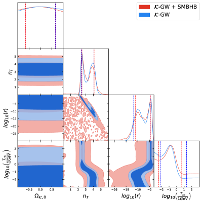
Figure 1: Marginalized 68% and 95% CL contours, and posterior distributions, for the free parameters of the $\mathcal{K}$-GW and $\mathcal{K}$-GW + SMBHB models. The dashed lines enclose the $1\sigma$ regions.

In Fig. 1, we show the $1\sigma$-$2\sigma$ contour plots and the posterior distributions for the $\mathcal{K}$-GW spectrum and the combined spectrum originating from inflation plus the SMBHB signal. We can see that the behaviors of $\log_{10}(r)$, $n_{T}$ and $\log_{10}(T_{\text{rh}}/1\,\text{GeV})$ are analogous to those emerged from the analysis of NANOGrav Afzal et al. (2023). Specifically, we note a strong covariance between the $n_{T}$ and $\log_{10}(r)$, and a bimodal distribution for both the marginalized posteriors. These features remain unchanged for the $\mathcal{K}$-GW and $\mathcal{K}$-GW + SMBHB spectra, respectively. In the 2D contour plots of the pairs $\{\log_{10}(T_{\text{rh}}/1\,\text{GeV}),n_{T}\}$ and $\{\log_{10}(T_{\text{rh}}/1\,\text{GeV}),\log_{10}(r)\}$, the bimodality induces a reflection symmetry with respect to the points $(-0.6,3.25)$ and $(-0.6,-6)$ in the $\{\log_{10}(T_{\text{rh}}/1\,\text{GeV}),n_{T}\}$ and $\{\log_{10}(T_{\text{rh}}/1\,\text{GeV}),\log_{10}(r)\}$ planes, respectively. In analogy with the analysis made in Ref. Agazie et al. (2023b), we highlight two regimes: $T\ll 1$ GeV and $T\gg 1$ GeV. In the first one, the reheating frequency $f_{\text{rh}}$ is below the PTA frequencies and the GW spectrum in the observed band is composed of tensor modes that re-entered the horizon during reheating after inflation. The second regime is characterized by a $f_{\text{rh}}$ greater than the frequencies in the PTA band. In this case, the GW spectrum comprises tensor modes that re-entered the horizon during the radiation era. Our results indicate that the spatial curvature parameter is constrained to $\Omega_{\mathcal{K},0}=0.00\pm 0.67$ at the 68% confidence level (CL).

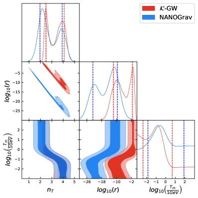
Figure 2: Comparison between the 68% and 95% CL results of our analysis and those of the NANOGrav collaboration Agazie et al. (2023b).

In Fig. 2, we compare the results on the common parameters of the $\mathcal{K}$-GW scenario and the cosmic inflation spectrum considered by NANOGrav, i.e., $\log_{10}(r)$, $n_{T}$ and $\log_{10}(T_{\text{rh}}/1\,\text{GeV})$. A common feature of both models is the bimodal distributions for $\log_{10}(r)$ and $n_{T}$, leading to two different regimes for $T_{\text{rh}}$. Nevertheless, we notice that the posterior distribution of $\log_{10}(r)$ in our model is shifted with respect to the NANOGrav findings, resulting in a factor of $\sim 10^{11}$ discrepancy for the most likely values of $r$. However, both estimates agree with the Planck constraint, namely $r<0.06$ Akrami et al. (2020). Moreover, the NANOGrav collaboration constrains the value of the strain amplitude to $2.4^{+0.7}_{-0.6}\times 10^{-15}$ at a reference frequency of 1 yr^-1 Agazie et al. (2023a). This bound induces a limit on the spectral index $n_{T}$. Specifically, when $T\ll 1$ GeV we recover the peak at $n_{T}=4$ in the posterior distribution, in analogy with the NANOGrav analysis Afzal et al. (2023). On the other hand, when $T\gg 1$ GeV, we find a peak at $n_{T}=2.5$, while the NANOGrav posterior shows a peak at $n_{T}=2$ Afzal et al. (2023).

Furthermore, we analyze the case when a Gaussian prior is imposed on $\Omega_{\mathcal{K},0}$. In particular, for the mean and the variance of the Gaussian distribution, we consider the best-fit and the 99% CL values obtained by Planck, i.e., $-0.06$ and $0.18$, respectively Akrami et al. (2020). In Fig. 3, we thus compare the results for the $\mathcal{K}$-GW spectrum in the case of uniform and Gaussian priors on $\Omega_{\mathcal{K},0}$. We note that the values of $\log_{10}(r)$, $n_{T}$ and $\log_{10}(T_{\text{rh}}/1\,\text{GeV})$ are quite independent from the prior on $\Omega_{\mathcal{K},0}$, as the corresponding 1D posterior distributions and the 2D contours overlap. On the other hand, such analysis allows us to improve the accuracy on $\Omega_{\mathcal{K},0}$ by a factor $\sim 4$: $\Omega_{\mathcal{K},0}=-0.05\pm 0.17$ (68% CL). The latter shows the significant role played by the priors in the present analysis.

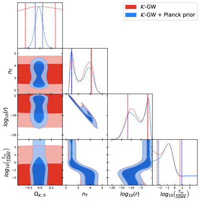
Figure 3: Comparison between the 68% and 95% CL results obtained by assuming a uniform (red) and a Gaussian (blue) prior on $\Omega_{\mathcal{K},0}$. The latter is based on the constraint given by the Planck collaboration Akrami et al. (2020).

V.1 Consistency checks

Here, we conduct two consistency checks to validate our study and ensure the absence of possible numerical artifacts in our analysis.

We first examine the impact of our $h$ assumption. In the main analysis, we set $h=0.67$, in agreement with the Planck result Akrami et al. (2020). On the other hand, one may consider the direct measurement of the Hubble constant based on local Cepheids Riess et al. (2022). In this case, we can assume $h=0.73$ and compare the posterior distributions obtained with the two different values of the Hubble constant (see Fig. 4). We notice that the choice of $\mathcal{H}_{0}$ does not actually affect our results.

The second check consists of fixing $\Omega_{\mathcal{K},0}=0$ in the $\mathcal{K}$-GW model. As shown in Fig. 5, the contours and the posterior distributions fully overlap with the NANOGrav results that were obtained in the case of vanishing spatial curvature. Once again, this confirms the goodness of our analysis and, therefore, validates the new findings related to the non-flat universe scenario.

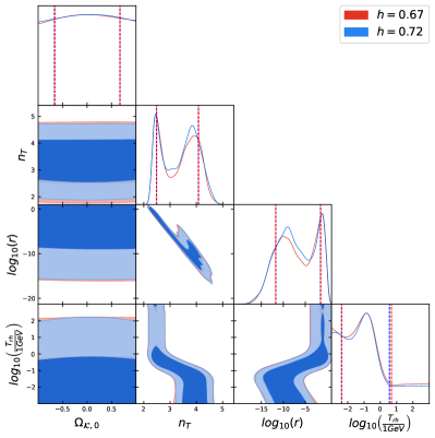
Figure 4: Marginalized 68% and 95% CL contours, and posterior distributions, for the free parameters of the $\mathcal{K}$-GW model under different assumptions for $h$.

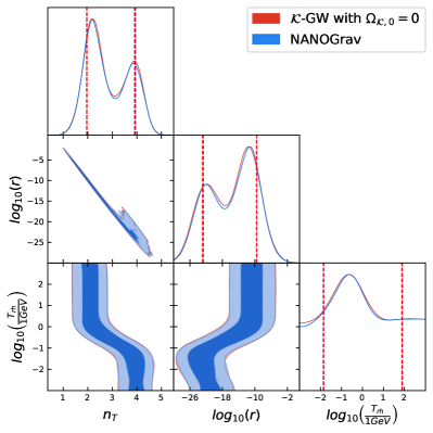
Figure 5: Comparison between the 68% and 95% CL predictions of the $\mathcal{K}$-GW model with $\Omega_{\mathcal{K},0}=0$ and the results of the NANOGrav collaboration Agazie et al. (2023b).

VI Final remarks

In this study, we investigated primordial GWs that originated during inflation and their propagation in the subsequent radiation and matter epochs. Specifically, we considered the solutions to the Friedmann equations for an isotropic and homogeneous background universe with non-vanishing spatial curvature. Then, we introduced linear tensor perturbations around the FLRW metric to account for the GW evolution under different universe’s geometry. With the help of transfer functions and suitable initial conditions, we obtained the energy density and the power spectrum of primordial GWs.

Therefore, we proposed a new parametrization of the tensor power spectrum that includes a correction factor due to the presence of non-zero spatial curvature, in addition to the tensor-to-scalar ratio and the spectral index typical of the standard flat scenario. We then expressed the relic GW energy density in terms of effective degrees of freedom contributing to the entropy and density of relativistic particles. Moreover, we considered the modifications in the spectral shape induced by the radiation-matter equivalence and the reheating phase.

Given the above theoretical scenario, we revisited the constraints on spatial curvature in light of the recent observations of a stochastic GWB. For this purpose, we employed the NANOGrav 15-year dataset release and performed a Bayesian analysis of the newly proposed parametrization of the tensor power spectrum. In particular, assuming uniform flat priors on the free parameters of the models, we found $\Omega_{\mathcal{K},0}=0.00\pm 0.67$ (68% CL). Therefore, to effectively constrain the geometry of the universe, we assumed a $3\sigma$ Planck prior on $\Omega_{\mathcal{K},0}$. In doing so, we obtained $\Omega_{\mathcal{K},0}=-0.05\pm 0.17$ (68% CL). Furthermore, we found bimodal distributions for both $\log_{10}r$ and $n_{T}$, whose behaviors are analogous to those obtained by the NANOGrav collaboration. However, our posterior on $\log_{10}r$ is shifted with respect to the NANOGrav results by several orders of magnitude. Nevertheless, our results on $r$ are in agreement with the Planck-CMB limits.

Finally, we carried out some consistency checks to validate our results. First, we investigated the impact of the Hubble constant value on the final numerical outcomes. Specifically, we showed that the same conclusions can be achieved by either assuming the Planck value or the local estimate for $\mathcal{H}_{0}$. Then, we examined potential numerical artifacts by analyzing our GWB model under the assumption of vanishing curvature. In doing so, we replicated the NANOGrav results, thereby confirming the validity of the new findings associated with the non-flat universe scenario.

In the context of recent debates on possible evidence of non-zero curvature, the present study provides further support for a flat universe, in agreement with the standard predictions of the CMB anisotropies. In conclusion, it is important to note that our findings are derived from a simplified power-law form of the tensor power spectrum. Exploring more sophisticated cases would be interesting to validate the current results. Additionally, while at present the NANOGrav observations alone seem to have a marginal impact on constraining spatial curvature, future releases of PTA data in the coming years may enhance the accuracy of all background parameters.