Fourier Transform-based Estimators for Data Sketches

Abstract

In this paper we consider the problem of estimating the $f$-moment ($\sum_{v\in[n]}(f(\mathbf{x}(v))-f(0))$) of a dynamic vector $\mathbf{x}\in\mathbb{G}^{n}$ over some abelian group $(\mathbb{G},+)$, where the $\|f\|_{\infty}$ norm is bounded. We propose a simple sketch and new estimation framework based on the Fourier transform of $f$. I.e., we decompose $f$ into a linear combination of homomorphisms $f_{1},f_{2},\ldots$ from $(\mathbb{G},+)$ to $(\mathbb{C},\times)$, estimate the $f_{k}$-moment for each $f_{k}$, and synthesize them to obtain an estimate of the $f$-moment. Our estimators are asymptotically unbiased and have variance asymptotic to $\|\mathbf{x}\|_{0}^{2}(\|f\|_{\infty}^{2}m^{-1}+\|\hat{f}\|_{1}^{2}m^{-2})$, where the size of the sketch is $O(m\log n\log|\mathbb{G}|)$ bits.

When $\mathbb{G}=\mathbb{Z}$ this problem can also be solved using off-the-shelf $\ell_{0}$-samplers with space $O(m\log^{2}n)$ bits, which does not obviously generalize to finite groups. As a concrete benchmark, we extend [26]’s singleton-detector-based sampler to work over $\mathbb{G}$ using $O(m\log n\log|\mathbb{G}|\log(m\log n))$ bits.

We give some experimental evidence that the Fourier-based estimation framework is significantly more accurate than sampling-based approaches at the same memory footprint.

1 Introduction

We consider the problem of maintaining a linear sketch of a dynamic vector $\textbf{x}\in\mathbb{G}^{n}$, initially $0^{n}$, where $\mathbb{G}$ is an additive abelian group and 0 its identity element. It is subject to coordinate updates:

$$\mathsf{Update}(v,y):\text{Set $\mathbf{x}(v)\leftarrow\mathbf{x}(v)+y$, where $v\in[n],y\in\mathbb{G}$.}$$

Our ambition is to sketch $\mathbf{x}$ so as to facilitate the estimation of any $f$-moment, with finite $\|f\|_{\infty}$, defined as

$$\sum_{v\in[n]}(f(\mathbf{x}(v))-f(0)),\text{ where $f:\mathbb{G}\to\mathbb{C}$.}$$

We can rewrite the $f$-moment as $\lambda(\mathbb{E}f(\mathbf{x}(I))-f(0))$, where $\lambda=|\operatorname{supp}(\mathbf{x})|=\|\mathbf{x}\|_{0}=|\{v\mid\mathbf{x}(v)\neq 0\}|$ is the support size of $\mathbf{x}$ and $I$ is a uniform random index drawn from $\operatorname{supp}(\mathbf{x})$. With a generic abelian group $\mathbb{G}$, this definition considerably generalizes the $f$-moment estimation problem classically defined in the turnstile model (the case $\mathbb{G}=\mathbb{Z}$). The motivation for this generalization are discussed in Section 1.4.

When $\|f\|_{\infty}$ is bounded, a “universal” solution is to take a sample $S$ from $\operatorname{supp}(\mathbf{x})$ and estimate $\mathbb{E}f(\mathbf{x}(I))$ by taking the empirical mean of $\{f(\mathbf{x}(v))\}_{v\in S}$; $\lambda$ can be estimated separately. This scheme is unbiased and has variance $O(\lambda^{2}\|f\|_{\infty}^{2}/|S|)$. To determine a comparison baseline, we briefly discuss how such a sample set $S$ can be constructed.

• It is tempting to use the classic methods like reservoir sampling [45] and $k$-min sampling [11], which can sample an index uniformly from the support over a stream with $O(\log n+\log|\mathbb{G}|)$ bits: $O(\log n)$ to store the index and hash value and $O(\log|\mathbb{G}|)$ to aggregate the updates. However, since we are considering general group-valued updates, an $\mathsf{Update}(v,y)$ can be undone by another $\mathsf{Update}(v,-y)$. The incremental-setting samplers [45, 11] cannot be used.

• In the turnstile model with $\mathbb{G}=\mathbb{Z}$, the sample set $S$ can be obtained with $\ell_{0}$-samplers; see the survey of Cormode and Firmani [18]. An $\ell_{0}$-sampler returns a pair $(u,\mathbf{x}(u))$, where $u\in[n]$ is drawn uniformly at random from the support $\operatorname{supp}(\mathbf{x})$. When $\mathbf{x}$ is integer-valued with each component $\mathbf{x}(u)$ in $[-n,n]$, both $u,\mathbf{x}(u)$ require $O(\log n)$ bits, leading to $O(\log^{2}n)$ bits of space for the $\ell_{0}$ sampler [18]. However, there is no obvious way to generalize the $\ell_{0}$-samplers to work over finite groups.

• For an arbitrary group $\mathbb{G}$ we can use a generalization of the singleton-detection method in [26], which is weaker than an $\ell_{0}$-sampler in that we only learn $\mathbf{x}(u)$ ($\log|\mathbb{G}|$ bits), $u$ uniformly random from $\operatorname{supp}(\mathbf{x})$, rather than also learn the index $u$ ($\log n$ bits). The data structure works as follows. We sample index sets $\mathcal{I}_{k}\subset[n]$, $k\in[\log n]$ with probability $2^{-k}$ and choose a certain hash function $H:[n]\times\mathbb{G}\to\mathbb{G}^{O(r)}$ that outputs a vector of $\mathbb{G}$-valued variables. The data structure stores an array $\operatorname{DetectionBucket}$, initially all zero, and implements $\mathsf{Update}(v,y)$ as follows. For each $k\in[\log n]$, if $v\in\mathcal{I}_{k}$, set

  $$\operatorname{DetectionBucket}[k]\leftarrow\operatorname{DetectionBucket}[k]+H(v,y),$$

  where ‘$+$’ is component-wise addition in $\mathbb{G}$.

  Theorem 1.1.

  Let the set of indices hashed to $\operatorname{DetectionBucket}[k]$ be ${\mathcal{I}}_{k}^{\prime}=\mathcal{I}_{k}\cap\operatorname{supp}(\mathbf{x})$. There is $H$ such that $\operatorname{DetectionBucket}[k]$ can be interpreted with the following guarantees. If $|\mathcal{I}_{k}^{\prime}|=1$, it reports $\mathtt{singleton}$ with probability 1, as well as its $\mathbb{G}$-value. If $|\mathcal{I}_{k}^{\prime}|\neq 1$, it reports $\mathtt{not}\text{-}\mathtt{singleton}$ with probability at least $1-2^{-\Omega(r)}$ and falsely reports $\mathtt{singleton}$ with an arbitrary $\mathbb{G}$-value with probability at most $2^{-\Omega(r)}$. More precisely:

  • When $|\mathbb{G}|$ is odd, there is $H:[n]\times\mathbb{G}\to\mathbb{G}^{2r}$ such that the false-positive probability is at most $(3/4)^{r}$.

  • When $|\mathbb{G}|$ is even, there is $H:[n]\times\mathbb{G}\to\mathbb{G}^{3r}$ such that the false-positive probability is at most $(8/9)^{r}$.

  See the Appendix A for proof.

With the discussion above, to achieve variance $O(\lambda^{2}\|f\|_{\infty}^{2}/m)$ for the $f$-moment estimation problem over $\mathbb{G}$, the sampling-based solution needs either $O(m\log^{2}n)$ bits for large groups (e.g., $\mathbb{G}=\mathbb{Z}$) using $\ell_{0}$-samplers, or $O(m\log n\log|\mathbb{G}|\log(\delta^{-1}\log n)))$ bits using Theorem A.1, which introduces a bias of $O(\delta\lambda\|f\|_{\infty})$ due to false positives. To preserve the asymptotic variance, we need to set $\delta<1/\sqrt{m}$, so the actual size is $O(m\log n\log|\mathbb{G}|\log(m\log n))$ bits. The sampling-based solution is wasteful and unsatisfactory, since, by design, all of the data stored in bucket locations that do not isolate a singleton are ignored, while the overhead dedicated to singleton-detection is a significant factor $\Theta(\log(m\log n))$.

In this paper we take a totally different approach to estimating $f$-moments over a generic abelian group $\mathbb{G}$, without any $\ell_{0}$ sampling or singleton detection. All the data stored in the sketch contributes to the estimation. We give a satisfactory answer to the question: how should a bucket be interpreted, given that an unknown number of indices have been hashed to it?

1.1 Insight and Overview

Without the singleton-detection part, one may simply store the $\mathbb{G}$-valued array $\operatorname{Bucket}$, initially all zero. Upon $\mathsf{Update}(v,y)$, for each $k\in[\log n]$,

$$\operatorname{Bucket}[k]\leftarrow\operatorname{Bucket}[k]+y\cdot\mathbbm{1}\left[{v\in\mathcal{I}_{k}}\right].$$

By construction, a plain $\operatorname{Bucket}[k]$ stores the $\mathbb{G}$-valued variable $X$ obtained by taking a sample $\mathcal{I}_{k}\subseteq[n]$ with probability $p=2^{-k}$ and summing: $X=\sum_{v\in\mathcal{I}_{k}}\mathbf{x}(v)$. When $k$ and $\lambda=\|x\|_{0}$ are large, $|\mathcal{I}_{k}|\sim\operatorname{Poisson}(p\lambda)$ tends to a Poisson distribution. For simplicity, we we shall assume that $|\mathcal{I}_{k}|\sim\operatorname{Poisson}(p\lambda)$ is selected, then $|\mathcal{I}_{k}|$ indices $\{I_{j}\}_{1\leq j\leq|\mathcal{I}_{k}|}$ are selected uniformly at random from $\operatorname{supp}(\mathbf{x})$ with replacement, so $X$ is precisely

$$X=\sum_{j=1}^{\mathrm{Poisson}(p\lambda)}\mathbf{x}(I_{j}).$$

The goal is to estimate the $f$-moment $\lambda(\mathbb{E}f(\mathbf{x}(I))-f(0))$ from the observation $X$. We begin with the trivial but important observation that when $f$ is linear, $X$ betrays lots of useful information about $\mathbb{E}f(\mathbf{x}(I))$. In particular,

$$\mathbb{E}f(X)=\mathbb{E}f\left(\sum_{j=1}^{\mathrm{Poisson}(p\lambda)}\mathbf{x}(I_{j})\right) =\mathbb{E}\sum_{j=1}^{\mathrm{Poisson}(p\lambda)}f\left(\mathbf{x}(I_{j})\right) f \star$$ from the linearity of ()

$$=p\lambda\mathbb{E}f(\mathbf{x}(I)).$$ linearity of expectation

Thus $f(X)/p$ is an unbiased estimator for $\lambda\mathbb{E}f(\mathbf{x}(I))$.

The key insight.

In the example above it is not important that $f$ is linear per se, but that it is a homomorphism (allowing the step $(\star)$), in this case from $(\mathbb{G},+)$ to $(\mathbb{C},+)$. Moreover, other homomorphisms are equally useful. For example, suppose that $f$ is instead a homomorphism from $(\mathbb{G},+)$ to $(\mathbb{C},\times)$, the multiplicative group of complex numbers, i.e., for any $x,y\in\mathbb{G}$, $f(x+y)=f(x)f(y)$. We can still infer information about $\mathbb{E}f(\mathbf{x}(I))$ from $f(X)$, even when $X$ is the sum of an unknown number of coordinates of $\mathbf{x}$, since $f(X)$ is just the product of $f(\mathbf{x}(I_{j}))$s. We compute $\mathbb{E}f(X)$ as follows.

$$\mathbb{E}f(X) =\mathbb{E}f\left(\sum_{j=1}^{\mathrm{Poisson}(p\lambda)}\mathbf{x}({I_{j}})\right)$$

$$=\mathbb{E}\prod_{j=1}^{\mathrm{Poisson}(p\lambda)}f\left(\mathbf{x}({I_{j}})\right) f:(\mathbb{G},+)\to(\mathbb{C},\times) \star\star$$ Since is a homomorphism ()

$$=e^{-p\lambda}\sum_{k=0}^{\infty}\frac{(p\lambda)^{k}}{k!}\mathbb{E}\prod_{j=1}^{k}f(\mathbf{x}({I_{j}})) \mathrm{Poisson}(p\lambda)$$ Definition of

$$=e^{-p\lambda}\sum_{k=0}^{\infty}\frac{(p\lambda)^{k}}{k!}(\mathbb{E}f(\mathbf{x}({I})))^{k} \mathbf{x}({I_{j}})$$ Since the s are i.i.d.

$$=e^{p\lambda(\mathbb{E}f(\mathbf{x}({I}))-1)} \text{Taylor expansion of $\exp(p\lambda\mathbb{E}f(\mathbf{x}(I)))$}.$$

Step ($\star\star$) allows us to extract useful information from $f(X)$ and convert it to an unbiased estimator of $\lambda(\mathbb{E}f(\mathbf{x}({I}))-1)$; see Section 4.

Now suppose that $f$ is some function that can be decomposed into a linear combination of homomorphisms $f_{1},f_{2},f_{3},\ldots$ from $(\mathbb{G},+)$ to $(\mathbb{C},\times)$. We can compute an estimation $\tilde{f}_{j}$ of the $f_{j}$-moment $\lambda(\mathbb{E}f_{j}(\mathbf{x}(I))-f_{j}(0))$ separately for each $j$ and thereby obtain an estimate $\tilde{f}$ of the $f$-moment $\lambda(\mathbb{E}f(\mathbf{x}(I))-f(0))$. See Figure 1 for a visualization of the estimation process. There is a perfect tool to decompose functions into a linear combination of homomorphisms, namely the Fourier transform.

Figure 1: Diagram of the $f$-moment estimation process. Decompose $f$ as $f_{1}+\ldots+f_{k}$ where $f_{j}$s are homomorphisms. For $j=1,\ldots,k$, compute $\tilde{f}_{j}$ that estimates the $f_{j}$-moment of $\mathbf{x}$, namely $\lambda(\mathbb{E}f_{j}(\mathbf{x}(I))-f_{j}(0))$. Then $\tilde{f}=\tilde{f}_{1}+\ldots+\tilde{f}_{k}$ is the estimator for the $f$-moment $\lambda(\mathbb{E}f(\mathbf{x}(I))-f(0))$.

1.2 Related Work

A recent paper by Chen, Indyk, and Woodruff [10] considers a similar problem, but in the incremental setting. Here sampling is straightforward; the main contribution is reducing the space per sample below $O(\log n)$ bits.

Our new framework is also relevant to the pursuit of universal sketches. Nelson [37] posed the general question of designing a single universal sketch for an integer vector $\mathbf{x}\in[-M,M]^{n}$ such that for any $f$ in some class $\mathscr{F}$, $f(\mathbf{x})$ could be $(\epsilon,\delta)$-approximated. Nelson’s question was answered in part by Braverman and Chestnut [6], who gave a universal sketch for all negative moments. Braverman and Ostrovsky [8] characterized which monotonically increasing functions $f$ with $f(0)=0$ have $\operatorname{poly}(\log n,\epsilon^{-1})$-space sketches to estimate $f$-moments of $\mathbf{x}\in\mathbb{N}^{n}$. Braverman, Chestnut, Woodruff, and Yang [7] further classified nearly all functions $f$—monotone or not—according to whether the $f$-moment of $\mathbf{x}\in\mathbb{Z}^{n}$, defined as $\sum_{v\in[n]}f(|\mathbf{x}(v)|)$, can be estimated from a space-efficient sketch.

We are not aware of any prior work on data sketches that use estimators based on Fourier transforms. Ganguly [25] and Kane, Nelson, Porat, and Woodruff [31] estimate $p$th momemts using random complex roots of unity, generalizing the way random signs are used in the AMS sketch [1] or Count-sketch [9]. However, we are not aware of any Fourier-theoretic interpretation of these sketches. Fourier analysis (on boolean functions) has been used to prove lower bounds on various sketching problems in graph streams [27, 44, 33, 34, 29, 30].

See Cormode and Firmani [18] for a survey of the literature [4, 19, 28, 36, 41] on $\ell_{0}$-samplers.

1.3 Model and Norms

We assume the random oracle model, i.e., the data structure has access to uniformly random hash functions. In this model the norm is to design estimators that are (asymptotically) unbiased; efficiency is measured by the tradeoff between the space of the sketch of the variance of the estimates. This is in contrast to the more common model in data sketching where random bits are freely available; all hash functions are explicit and contribute to the space bound. The data structure typically provides an $(\epsilon,\delta)$-accuracy guarantee, meaning the estimate is correct up to a $1\pm\epsilon$ factor with probability $1-\delta$. Space bounds are normally expressed in big-Oh notation, which often hides a non-trivial leading constant factor that is independent of the parameters, e.g., $\epsilon,\delta,n,\|\mathbf{x}\|_{0}$.

The one problem where both the random oracle and common model have a large body of work is the distinct elements/cardinality estimation problem. All of the practically influential sketches (HyperLogLog [21], PCSA [23], $k$-Min [12], non-mergeable sketches based on the Martingale transform [13, 43, 40], and recent variants of these [38, 17, 16, 42, 20, 35, 46]) are analyzed in the random oracle model. Sketches designed in the common model [2, 3, 32, 5] have significant leading constant factors. As our aim is to achieve reasonably practical algorithms with rigorous and precise guarantees, we work within the random oracle model and its associated norms.

1.4 New Results

Theorem 1.2.

Let $\mathbb{G}$ be any locally compact abelian group. Fix an accuracy parameter $m$. There is a linear sketch of a vector $\mathbf{x}\in\mathbb{G}^{n}$ occupying $O(m\ln n\log_{2}|\mathbb{G}|)$ bits, such that given any regular $f:\mathbb{G}\to\mathbb{C}$, we can estimate the $f$-moment $\sum_{v\in[n]}(f(\mathbf{x}(v))-f(0))$ with the following guarantees.

• The estimate is asymptotically unbiased. Its bias is $\lambda\|\hat{f}\|_{1}O(m^{-1})$, where $\lambda=\|\mathbf{x}\|_{0}$ and $\hat{f}$ is the Fourier transform of $f$.

• The variance of the estimate is $\lambda^{2}\left[\|f\|_{\infty}^{2}O(m^{-1})+\|\hat{f}\|_{1}^{2}O(m^{-2})\right]$.

Remark 1.

The update time for the sketch is $O(m\log n)$ and the time to estimate an $f$-moment is $O(m\log n\cdot|G|)$. When $\lambda>\operatorname{poly}(m)$ the update time can be reduced to $O(1)$; see Section 6. Even when $|\mathbb{G}|$ is infinite (say $\mathbb{Z}$), one usually has an upper bound on the magnitude of $\mathbf{x}$’s coordinates, so $\mathbf{x}$ is effectively in a (large) finite group.

Theorem 1.2 can be applied to a variety of situations. We give a couple of informal examples here, and give further detailed examples in Section 7.

Small groups: $\mathbb{Z}_{p}$.

We can think of sketching $\mathbf{x}\in\mathbb{Z}^{n}$ but doing the Fourier transform-based estimation in $\mathbb{G}=\mathbb{Z}_{p}$, or actually sketching $\mathbf{x}\in\mathbb{Z}_{p}^{n}$. The benefit of the former approach is flexibility: we can specify $p$ and $f:\mathbb{Z}_{p}\to\mathbb{C}$ at query time. The benefit of the latter approach is efficiency since we only need $O(m\ln n\log_{2}p)$ bits.

• Consider a system where users iteratively perform a sequence of transactions, each requiring $p$ distinct steps. Let $\mathbf{x}(u)$ be the number of steps taken by user $u$. To query the number of users in the middle of a transaction, we can estimate the $f$-moment with $f(j)=\mathbbm{1}\left[{j\not\equiv 0\pmod{p}}\right]$.

• Many real world data sets follow a power law distribution, and as a consequence are heavy tailed. For example, suppose $[n]$ is the space of Amazon products and $\mathbf{x}(v)$ the number of reviews for product $v$. Let us posit that at most 1% of the reviewed products have more than 127 reviews. If we are interested in the number of products with between 1 and 4 reviews, we can apply our framework with $\mathbb{G}=\mathbb{Z}_{128}$ and estimate the $f$-moment with $f(j)=\mathbbm{1}\left[{j\in[1,4]\pmod{128}}\right]$. The 1% of products with at least 128 reviews can perturb the estimate by 1% (pessimistically) or $\approx(4/128)$% (optimistically), if they are uniform modulo 128.

Product Groups.

Queries over multiple streams can be regarded as a higher order $f$-moment estimation, as mentioned in [7], where they reduce multiple integer streams to a single one via base-$b$ expansion. Our framework can handle queries on multiple streams natively, because if $\mathbb{G}$ is an LCA group, the direct product $\mathbb{G}^{k}$ is also an LCA group and we may execute the framework directly on the product stream.

• Suppose $\mathbf{x}_{1}(v)$ and $\mathbf{x}_{5}(v)$ are the number of 1-star and 5-star reviews for product $v$, and we wish to count the number of “controversial” products, with at least ten 1-star and ten 5-star reviews. We can form a sketch of the product stream $\mathbf{x}^{\prime}=((\mathbf{x}_{1}(v),\mathbf{x}_{5}(v)))_{v\in[n]}\in(\mathbb{Z}^{2})^{n}$ and apply the framework to $\mathbf{x}^{\prime}$ and $f:\mathbb{Z}\times\mathbb{Z}\to\mathbb{C}$, where $f(x,y)=\mathbbm{1}\left[{x\geq 10}\right]\mathbbm{1}\left[{y\geq 10}\right]$. The number of controversial products is equal to the $f$-moment, which can be estimated in our Fourier framework using the 2D Fourier transform.

• In principle the Fourier framework can be used to estimate the moment of any bounded function over any set of streams. For example, suppose a product has ten attributes and we want to estimate the number of products have at least five attributes that are greater than 100. This can be estimated by the Fourier estimator with $\mathbb{G}=\mathbb{Z}^{10}$ and $f:\mathbb{Z}^{10}\to\mathbb{C}$, $f(x_{1},x_{2},\ldots,x_{10})=\mathbbm{1}\left[{|\{k:x_{k}\geq 100\}|\geq 5}\right]$. This illustrates the expressive power of the framework. However, one should confirm that the variance is reasonable; in this case the variance is asymptotic to $\lambda^{2}\left[\|f\|_{\infty}^{2}O(m^{-1})+\|\hat{f}\|_{1}^{2}O(m^{-2})\right]$, where $\|f\|_{\infty}=1$ for any indicator function $f$ but $\|\hat{f}\|_{1}$ may be larger, depending on the structure of $f$; $\lambda$ is the support size of the product stream, i.e. the number of elements with at least one non-zero attribute. Thus, the estimator is only informative if the answer is reasonably large relative to $\lambda\left[O(m^{-1/2})+\|\hat{f}\|_{1}O(m^{-1})\right]$.

1.5 Organization

In Section 2 we review facts about groups, characters, and the Fourier transform. In Section 3 we present an abstract sketch called the Poisson tower. In Section 4 we first construct asymptotically unbiased estimators of the $\gamma$-moments, for any character $\gamma$, based on which we build the generic $f$-moment estimator. In Section 5 we analyze the variance of the $f$-moment estimator.

The abstract Poisson tower is an infinite-length vector. In Section 6 we define a natural truncation of the Poisson tower occupying $O(m\ln n\log_{2}|\mathbb{G}|)$ bits that has negligibly larger bias and variance. We also present a depoissonized version of the sketch (the binomial tower) that has fast $O(1)$ update time and negligibly larger bias/variance when $\lambda=\|\mathbf{x}\|_{0}=\Omega(\operatorname{poly}(m))$.

Section 7 illustrates a few applications of the Fourier transform-based estimators in various settings. Section 8 empirically compares the sampling-based method and the new Fourier-based method. We make some concluding remarks in Section 9.

Appendix A generalizes [26]’s singleton-detection to $\mathbb{G}$. Appendix B proves some useful mathematical lemmas. Appendix C and Appendix D give the full proofs of the theorems from Section 6.

2 Preliminaries: Groups, Characters, Fourier Transform

notation	definition	name
$\mathbb{Z}_{p}$	$(\mathbb{Z}/p\mathbb{Z},+)$	cyclic group of order $p$
$\mathbb{Z}$	$(\mathbb{Z},+)$	additive integer group
$\mathbb{R}$	$(\mathbb{R},+)$	additive real group
$\mathbb{T}$	$(\mathbb{R}/\mathbb{Z},+)$	unit circle

Table 1: Notations for common groups

As demonstrated in Section 1.4, a wide range of groups can be useful in practice. To concisely prove general results that apply to all groups of interest, we use the theory of Fourier analysis for locally compact abelian (LCA) groups (for reference, see for example [24]), which covers all the common choices of $\mathbb{G}$: $\mathbb{R},\mathbb{Z},\mathbb{T},\mathbb{Z}_{p},\mathbb{R}^{k},\mathbb{Z}^{k},\mathbb{T}^{k},\mathbb{Z}_{p}^{k}$. The notations are clarified in Table 1.

2.1 Fourier Transforms on LCA Groups

We start with the fundamental notion of character.

Definition 1 (character).

Let $(\mathbb{G},+)$ be an LCA group. A character $\gamma$ is a continuous function from $\mathbb{G}$ to $\mathbb{C}$ such that for any $x,y\in\mathbb{G}$, $\gamma(x+y)=\gamma(x)\gamma(y)$ and $|\gamma(x)|=1$.

Theorem 2.1 (Pontryagin duality, [24]).

Let $\mathbbold{\Gamma}$ be the set of characters of $\mathbb{G}$. $\mathbbold{\Gamma}$ is an LCA group with point-wise multiplication and the topology of local uniform convergence on compact sets. The character group of $\mathbb{G}$’s character group $\mathbbold{\Gamma}$ (i.e., the double dual of $\mathbb{G}$) is isomorphic to $\mathbb{G}$.

To emphasize this symmetry, we use the convention of using “$+$” as the operator in the group $\mathbbold{\Gamma}$ and writing $\gamma(x)$ as $\boldsymbol{(}{x},{\gamma}\boldsymbol{)}$ where $x\in\mathbb{G}$ and $\gamma\in\mathbbold{\Gamma}$. Thus for $\gamma,\gamma^{\prime}\in\mathbbold{\Gamma}$ and $x\in\mathbb{G}$, $\boldsymbol{(}{x},{\gamma+\gamma^{\prime}}\boldsymbol{)}=(\gamma+\gamma^{\prime})(x)=\gamma(x)\gamma^{\prime}(x)=\boldsymbol{(}{x},{\gamma}\boldsymbol{)}\boldsymbol{(}{x},{\gamma^{\prime}}\boldsymbol{)}$. Some common $(\mathbb{G},\mathbbold{\Gamma})$ pairs are listed as below.

• The character group of $\mathbb{Z}_{p}$ is $\mathbb{Z}_{p}$, where for $x\in\mathbb{Z}_{p}$ and $\gamma\in\mathbb{Z}_{p}$, $\boldsymbol{(}{x},{\gamma}\boldsymbol{)}=e^{2\pi x\gamma i/p}$.

• The character group of $\mathbb{Z}$ is $\mathbb{T}$, where for $x\in\mathbb{Z}$ and $\gamma\in\mathbb{T}$, $\boldsymbol{(}{x},{\gamma}\boldsymbol{)}=e^{2\pi x\gamma i}$.

• The character group of $\mathbb{R}$ is $\mathbb{R}$, where for $x\in\mathbb{R}$ and $\gamma\in\mathbb{R}$, $\boldsymbol{(}{x},{\gamma}\boldsymbol{)}=e^{2\pi x\gamma i}$.

• Let $\mathbb{G}_{1}$ and $\mathbb{G}_{2}$ be two LCA groups. The product group $\mathbb{G}_{1}\times\mathbb{G}_{2}$ is the set $\{(x,y):x\in\mathbb{G}_{1},y\in\mathbb{G}_{2}\}$ with entry-wise addition. Note that $\mathbb{G}_{1}\times\mathbb{G}_{2}$ is also an LCA group. The character group of $\mathbb{G}_{1}\times\mathbb{G}_{2}$ is $\mathbbold{\Gamma}_{1}\times\mathbbold{\Gamma}_{2}$ where for $x_{1}\in\mathbb{G}_{1},x_{2}\in\mathbb{G}_{2},\gamma_{1}\in\mathbbold{\Gamma}_{1},\gamma_{2}\in\mathbbold{\Gamma}_{2}$, $\boldsymbol{(}{(x_{1},x_{2})},{(\gamma_{1},\gamma_{2})}\boldsymbol{)}=\boldsymbol{(}{x_{1}},{\gamma_{1}}\boldsymbol{)}\boldsymbol{(}{x_{2}},{\gamma_{2}}\boldsymbol{)}$.

We list a few properties of characters that are used frequently later.

Proposition 1.

Let $x,y\in\mathbb{G}$ and $\gamma,\gamma^{\prime}\in\mathbbold{\Gamma}$. The following statements are true.

• $\boldsymbol{(}{x+y},{\gamma}\boldsymbol{)}=\boldsymbol{(}{x},{\gamma}\boldsymbol{)}\boldsymbol{(}{y},{\gamma}\boldsymbol{)}$.

• $\boldsymbol{(}{x},{\gamma+\gamma^{\prime}}\boldsymbol{)}=\boldsymbol{(}{x},{\gamma}\boldsymbol{)}\boldsymbol{(}{x},{\gamma^{\prime}}\boldsymbol{)}$.

• $|\boldsymbol{(}{x},{\gamma}\boldsymbol{)}|=1$.

• $\boldsymbol{(}{0},{\gamma}\boldsymbol{)}=\boldsymbol{(}{x},{0}\boldsymbol{)}=1$.

• $\boldsymbol{(}{-x},{\gamma}\boldsymbol{)}=\boldsymbol{(}{x},{-\gamma}\boldsymbol{)}=\overline{\boldsymbol{(}{x},{\gamma}\boldsymbol{)}}$, the complex conjugate of $\boldsymbol{(}{x},{\gamma}\boldsymbol{)}$.

The next important notion is the Haar measure.

Theorem 2.2 (Haar measure of LCA groups).

For any LCA group $\mathbb{G}$, there exists a unique (non-trivial) measure $\mu_{\mathbb{G}}$ (up to a multiplicative scalar) of $\mathbb{G}$ such that for any $x\in\mathbb{G}$ and measurable set $E\subset\mathbb{G}$,

$$\mu_{\mathbb{G}}(x+E)=\mu_{\mathbb{G}}(E),\mbox{ where $x+E$ is the translation of $E$ by $x$.}$$

For discrete groups, the Haar measure is just the counting measure. For $\mathbb{R}$ or $\mathbb{R}^{k}$, the Haar measure is just the usual Lebesgue measure. From now on, we will integrate over LCA groups with the Haar measure by default. Now we are ready to define the Fourier transform.

Definition 2 (Fourier transform).

Let $(\mathbb{G},+)$ be an LCA group. Let $f:\mathbb{G}\to\mathbb{C}$ such that $\int_{\mathbb{G}}|f|\,d\mu_{\mathbb{G}}<\infty$. We define the Fourier transform of $f$, $\hat{f}:\mathbbold{\Gamma}\to\mathbb{C}$ as follows. For any $\gamma\in\mathbbold{\Gamma}$,

$$\hat{f}(\gamma)=\int_{\mathbb{G}}f(x)\overline{\boldsymbol{(}{x},{\gamma}\boldsymbol{)}}\,d\mu_{\mathbb{G}}(x).$$

Definition 3 (regular functions).

A function $f:\mathbb{G}\to\mathbb{C}$ is regular if

• It is continuous and integrable, i.e., $\int_{\mathbb{G}}|f|\,d\mu_{\mathbb{G}}<\infty$,

• Its Fourier transform is integrable, i.e., $\int{\Gamma}|\hat{f}|\,d\mu{\Gamma}<\infty$.

Remark 2.

When $\mathbb{G}$ is finite, every function $f:\mathbb{G}\to\mathbb{C}$ is regular.

Theorem 2.3 (inverse Fourier transform, [24]).

Let $(\mathbb{G},+)$ be an LCA group. Then for any regular function $f$ and any $x\in\mathbb{G}$,

$$f(x)=\int{\Gamma}\hat{f}(\gamma)\boldsymbol{(}{x},{\gamma}\boldsymbol{)}\,d\mu{\Gamma}(\gamma),$$

with a proper normalization of the Haar measures $\mu_{\mathbb{G}}$ and $\mu{\Gamma}$.

Remark 3.

Neither our estimator nor its analysis depend on one specific normalization. It is only important to have them normalized, i.e., the inverse Fourier transform of the Fourier transform of a function $f$ goes back to $f$, instead of a multiple of $f$. In this work, we stick to the following conventions.

• Discrete Fourier Transform $(\mathbb{Z}_{p},\mathbb{Z}_{p})$. $\hat{f}(\gamma)=\sum_{x=0}^{p-1}f(x)e^{-2\pi x\gamma i/p}$; $f(x)=\frac{1}{p}\sum_{\gamma=0}^{p-1}\hat{f}(\gamma)e^{2\pi x\gamma i/p}$.

• Fourier Series $(\mathbb{Z},\mathbb{T})$. $\hat{f}(\gamma)=\sum_{x=-\infty}^{\infty}f(x)e^{-2\pi x\gamma i}$; $f(x)=\int_{-1/2}^{1/2}\hat{f}(\gamma)e^{2\pi x\gamma i}\,d\gamma$.

• Fourier Transform $(\mathbb{R},\mathbb{R})$. $\hat{f}(\gamma)=\int_{-\infty}^{\infty}f(x)e^{-2\pi x\gamma i}\,dx$; $f(x)=\int_{-\infty}^{\infty}\hat{f}(\gamma)e^{2\pi x\gamma i}\,d\gamma$.

2.2 Norms, Variance, and Covariance

Recall that for $\mathbf{x}\in\mathbb{G}^{n}$, $\|\mathbf{x}\|_{0}=\sum_{j=1}^{n}\mathbbm{1}\left[{\mathbf{x}(j)\neq 0}\right]$ is the number of non-zeros in $\mathbf{x}$. For function $f:\mathbb{G}\to\mathbb{C}$, where $\mathbb{G}$ is an LCA group, we define

$$\|f\|_{1} =\int_{\mathbb{G}}|f(x)|\,d\mu_{\mathbb{G}}(x) \|f\|_{\infty} =\sup_{x\in\mathbb{G}}|f(x)|.$$

Lemma 2.4.

If $f$ is regular, then $\|f\|_{\infty}\leq\|\hat{f}\|_{1}$.

Proof.

By the inverse Fourier transform (Theorem 2.3) and $|(x,\gamma)|=1$, we have, for any $x\in\mathbb{G}$,

$$\hskip 22.76228pt|f(x)|=\left|\int{\Gamma}\hat{f}(\gamma)\boldsymbol{(}{x},{\gamma}\boldsymbol{)}\,d\mu{\Gamma}(\gamma)\right| \leq\int{\Gamma}|\hat{f}(\gamma)||\boldsymbol{(}{x},{\gamma}\boldsymbol{)}|\,d\mu{\Gamma}(\gamma)=\int{\Gamma}|\hat{f}(\gamma)|\,d\mu{\Gamma}(\gamma)=\|\hat{f}\|_{1}.\hskip 22.76228pt\qed$$

The variance and covariance of complex random variables $X,Y$ are defined to be

$$\mathbb{V}X =\mathbb{E}\left((X-\mathbb{E}X)\overline{(X-\mathbb{E}X)}\right), \mathrm{Cov}(X,Y) =\mathbb{E}\left((X-\mathbb{E}X)\overline{(Y-\mathbb{E}Y)}\right).$$

3 The Poisson Tower Sketch

We first describe an abstract sketch, the Poisson tower. It is parameterized by a single integer $m$, which controls the variance of the estimates, and consists of an infinite vector $(X_{j})_{j\in\mathbb{Z}}$ of $\mathbb{G}$-valued cells, initialized as $0^{\mathbb{Z}}$. We think of cell $j$ having size $e^{-j/m}$. Each coordinate of the vector $\mathbf{x}(v)$ contributes a $Z_{v,j}\sim\operatorname{Poisson}(e^{-j/m})$ number of copies to cell $j$, where the $(Z_{v,j})_{v,j}$ random variables are independent, and assigned by the random oracle. In other words, $\mathsf{Update}(v,y)$ is implemented as follows.

$\mathsf{Update}(v,y)$:

For each $j\in\mathbb{Z}$, set $X_{j}\leftarrow X_{j}+Z_{v,j}y$, where $Z_{v,j}$s are independent $\mathrm{Poisson}(e^{-j/m})$ random variables.

Let $\mathbf{x}\in\mathbb{G}^{n}$ be the final vector after all updates. It is clear that

$$X_{j}=\sum_{v=1}^{n}Z_{v,j}\mathbf{x}(v).$$ (1)

We first design and analyze an estimator for the infinite sketch $(X_{j})_{j\in\mathbb{Z}}$, then consider a finite truncated version of the sketch with $O(m\ln n)$ cells. (When $j\gg m\ln n$, $X_{j}$ is usually 0, and when $j\ll m\ln\|\mathbf{x}\|_{0}-\Theta(m\ln m)$, $X_{j}$ contains little useful information.) The error introduced by truncation is negligible; it is analyzed in Section 6.1. We also analyze a further simplification in Section 6.2, where each coordinate $\mathbf{x}(v)$ only influences a single (random) cell $X_{j}$, so $\mathsf{Update}(v,y)$ takes $O(1)$ update time.

Theorem 3.1.

Let $(X_{j})_{j\in\mathbb{Z}}$ be a Poisson tower. Let $I$ be a uniformly random index from $\operatorname{supp}(\mathbf{x})$. Then $X_{j}\sim\sum_{r=1}^{\mathrm{Poisson}(\|\mathbf{x}\|_{0}e^{-j/m})}{\mathbf{x}({I_{r}})}$, where the $I_{r}$s are i.i.d. copies of $I$. In addition, $(X_{j})_{j\in\mathbb{Z}}$ are mutually independent.

Proof.

By Eq. 1, all $X_{j}$s are independent since all $Z_{v,j}$s are independent. Now we fix a $j\in\mathbb{Z}$. By a property of the Poisson distribution, if one independently draws a coordinate from $\|x\|_{0}$ non-zero coordinates, with replacement, $\mathrm{Poisson}(e^{-j/m}\|x\|_{0})$ number of times, then each non-zero coordinate is drawn $\mathrm{Poisson}(e^{-j/m})$ number of times and the number of times the coordinate gets drawn are mutually independent. Thus, since $0$ entries do not contribute to the sum,

$${\hskip 62.59596pt}\sum_{r=1}^{\mathrm{Poisson}(\|\mathbf{x}\|_{0}e^{-j/m})}{\mathbf{x}({I_{r}})} \sim\sum_{v\in[n];\mathbf{x}(v)\neq 0}Z_{v,j}\mathbf{x}(v)=\sum_{v\in[n]}Z_{v,j}\mathbf{x}(v)=X_{j}.\hskip 62.59596pt\qed$$

With this characterization theorem, to estimate the $f$-moment of $\mathbf{x}$ from the Poisson tower sketch, it suffices to solve the following estimation problem.

Problem 1 (Poisson tower estimation).

The problem has parameters $(R,\mathbb{G},m,\lambda,f)$, where $\mathbb{G}$ is a LCA group, $R$ is a $\mathbb{G}$-valued non-zero random variable with probability measure $\mu_{R}$, $m\in\mathbb{N}$, $\lambda\in\mathbb{R}^{+}$, and $f$ is a regular function over $\mathbb{G}$.

Input:

Observe an infinite $\mathbb{G}$-vector $(X_{j})_{j\in\mathbb{Z}}$, where $X_{j}$s are independent and for each index $j$, $X_{j}\sim\sum_{r=1}^{\mathrm{Poisson}(\lambda e^{-j/m})}R_{j,r}$, where $R_{j,r}$s are i.i.d. copies of $R$.

Output:

Estimate the $f$-moment $\lambda(\mathbb{E}f(R)-f(0))$.

Remark 4.

For the Poisson tower estimation problem, we will construct an estimator that works for for a generic non-zero random variable $R$, which is more than enough to estimate the $f$-moment of stream. Indeed, given a dynamic vector $\mathbf{x}\in\mathbb{G}^{n}$, just set $R=\mathbf{x}(I)$ (i.e., $R$ is a random non-zero coordinate in the vector $\mathbf{x}$) and the estimator will estimate $\lambda(\mathbb{E}f(\mathbf{x}(I))-f(0))=\sum_{v\in[n]}(f(\mathbf{x}(v))-f(0))$, which is precisely the $f$-moment of the stream.

In Section 4 we construct estimators for the Poisson tower estimation problem following the steps described in Fig. 1.

4 Construction of the Unbiased Estimators

The first step is to construct an unbiased estimator for characters. Fix any character $\gamma\in\mathbbold{\Gamma}$ in the character group of $\mathbb{G}$. The goal is to construct an unbiased estimator for the $\gamma$-moment:

$$\lambda(\mathbb{E}\boldsymbol{(}{R},{\gamma}\boldsymbol{)}-\boldsymbol{(}{0},{\gamma}\boldsymbol{)}) =\lambda(\mathbb{E}\boldsymbol{(}{R},{\gamma}\boldsymbol{)}-1).$$

Theorem 4.1.

For any $\gamma$ in the character group $\mathbbold{\Gamma}$, $\mathbb{E}\boldsymbol{(}{X_{j}},{\gamma}\boldsymbol{)}=\exp\left(e^{-j/m}\lambda(\mathbb{E}\boldsymbol{(}{R},{\gamma}\boldsymbol{)}-1)\right)$.

Proof.

By definition, the character is a homomorphism from $(\mathbb{G},+)$ to $(\mathbb{C},\times)$. Thus the computation around ($\star\star$) in Section 1.1 gives

$${\hskip 59.75095pt}\mathbb{E}\boldsymbol{(}{X_{j}},{\gamma}\boldsymbol{)}=\mathbb{E}\boldsymbol{(}{\underbrace{\sum_{v=1}^{\mathrm{Poisson}(\lambda e^{-j/m})}R_{j,v}}_{X_{j}}},{\;\gamma}\boldsymbol{)}=\exp\left(\lambda e^{-j/m}(\mathbb{E}\boldsymbol{(}{R},{\gamma}\boldsymbol{)}-1)\right).\hskip 59.75095pt\qed$$

We see the expectation of $\boldsymbol{(}{X_{j}},{\gamma}\boldsymbol{)}$ leaks information about the target $\lambda(\mathbb{E}\boldsymbol{(}{R},{\gamma}\boldsymbol{)}-1)$. Thus the next step is to aggregate the information from this whole bilaterally infinite vector $(X_{j})_{j\in\mathbb{Z}}$.

4.1 $(-1/3)$-Aggregation

Recall that $X_{j}$ is the value stored at cell $j$, which has “size” $e^{-j/m}$. Following an idea from the recent cardinality estimators of [46], we will aggregate all the cells weighted by the $\tau$th power of its size, i.e., $e^{-\tau j/m}$.

Definition 4 ($(-1/3)$-aggregation).

For any $\gamma\in\mathbbold{\Gamma}$, define

$$U_{\gamma}=\sum_{k=-\infty}^{\infty}(\boldsymbol{(}{X_{k}},{\gamma}\boldsymbol{)}-1)e^{\frac{1}{3}k/m}.$$

Remark 5.

We briefly explain the intuition for choosing the statistic $U_{\gamma}$. By Theorem 4.1, we know $\boldsymbol{(}{X_{k}},{\gamma}\boldsymbol{)}$ is an informative statistic of $\lambda(\mathbb{E}\boldsymbol{(}{R},{\gamma}\boldsymbol{)}-1)$ which is exactly the $\gamma$-moment. A naive $\tau$-GRA [46] style aggregation gives $U^{\prime}=\sum_{k=-\infty}^{\infty}\boldsymbol{(}{X_{k}},{\gamma}\boldsymbol{)}e^{-\tau k/m}$. However $U^{\prime}$ does not absolutely converge for any $\tau\in\mathbb{R}$ because $\boldsymbol{(}{X_{k}},{\gamma}\boldsymbol{)}\to 1$ as $k\to\infty$ and goes to random noise as $k\to-\infty$. To fix this, we replace $\boldsymbol{(}{X_{k}},{\gamma}\boldsymbol{)}$ by $(\boldsymbol{(}{X_{k}},{\gamma}\boldsymbol{)}-1)$ so that $(\boldsymbol{(}{X_{k}},{\gamma}\boldsymbol{)}-1)\to 0$ as $k\to\infty$. Now for $\sum_{k=-\infty}^{\infty}(\boldsymbol{(}{X_{k}},{\gamma}\boldsymbol{)}-1)e^{-\tau k/m}$ to converge, we have to pick a negative $\tau$ to suppress the random noise as $k\to-\infty$. However, given $\tau$ is negative, $e^{-\tau k/m}$ grows exponentially as $k\to\infty$, which has to be suppressed by $(\boldsymbol{(}{X_{k}},{\gamma}\boldsymbol{)}-1)$. As we see later, to keep the first and second moments of $U_{\gamma}$ bounded, we must have $\tau\in(-1/2,0)$ Furthermore, it is algorithmically convenient for $\tau$ to be the reciprocal of an integer. Therefore, we choose $\tau=-1/3$.

As a sanity check, we show that the statistic $U_{\gamma}$ is finite.

Theorem 4.2.

$U_{\gamma}$ converges absolutely almost surely. Furthermore, $\sup_{\gamma\in\mathbbold{\Gamma}}|U_{\gamma}|$ is finite almost surely.

Proof.

Note that since $\boldsymbol{(}{0},{\gamma}\boldsymbol{)}=1$,

$$\sum_{k=-\infty}^{\infty}|\boldsymbol{(}{X_{k}},{\gamma}\boldsymbol{)}-1|e^{\frac{1}{3}k/m} \leq\sum_{k=-\infty}^{\infty}2\cdot\mathbbm{1}\left[{X_{k}\neq 0}\right]e^{\frac{1}{3}k/m}=A+B,$$

where

$$A=\sum_{k=-\infty}^{0}2\cdot\mathbbm{1}\left[{X_{k}\neq 0}\right]e^{\frac{1}{3}k/m}\quad\quad\text{ and }\quad\quad B=\sum_{k=1}^{\infty}2\cdot\mathbbm{1}\left[{X_{k}\neq 0}\right]e^{\frac{1}{3}k/m}.$$

$A$ is finite since $\sum_{k=-\infty}^{0}|2\cdot\mathbbm{1}\left[{X_{k}\neq 0}\right]e^{\frac{1}{3}k/m}|\leq\sum_{k=-\infty}^{0}2e^{\frac{1}{3}k/m}<\infty.$ We now prove there are only finitely many non-zero terms in $B$ a.s. (almost surely). $X_{k}$ is the sum of $Z$ number of i.i.d. copies of $R$s, where $Z\sim\mathrm{Poisson}(\lambda e^{-k/m})$. Thus $X_{k}\neq 0$ implies $Z>0$. Then we have $\mathbb{P}(X_{k}\neq 0)\leq\mathbb{P}(Z>0)=1-e^{-\lambda e^{-k/m}}<\lambda e^{-k/m}$. Thus $\sum_{k=1}^{\infty}\mathbb{P}(X_{k}\neq 0)\leq\sum_{k=1}^{\infty}\lambda e^{-k/m}<\infty.$ By Borel-Cantelli lemma, we conclude that only finitely many $X_{k}$s with $k\geq 1$ are non-zero a.s. Hence $B$ is a finite sum a.s. Now we know $A+B$ is finite a.s., which implies $U_{\gamma}$ converges absolutely a.s. Finally, note that $A$ and $B$ do not depend on $\gamma$. Thus a.s., we have for every $\gamma\in\mathbbold{\Gamma}$, $|U_{\gamma}|\leq A+B<\infty$. Thus $\sup_{\gamma\in\mathbbold{\Gamma}}|U_{\gamma}|$ is finite a.s. ∎

Next we are going to compute the mean of the $(-1/3)$-aggregation, i.e., $\mathbb{E}U_{\gamma}$.

4.2 Asymptotic Mean of $U_{\gamma}$

The mean of $U_{\gamma}$ is expressed in terms of the Gamma function $\Gamma$ (Fig. 2). This is not to be confused with the character group $\mathbbold{\Gamma}$, which is never treated as a function. In fact, the Pontryagin pair, usually denoted as $(G,\Gamma)$, is intentionally lifted bold $(\mathbb{G},\mathbbold{\Gamma})$ to avoid the symbol conflict with the Gamma function $\Gamma$.

Figure 2: Gamma function $\Gamma(x)$ over $(-1,0)\cup(0,1)$

Lemma 4.3.

For any $\gamma\in\mathbbold{\Gamma}$,

$$m^{-1}\mathbb{E}U_{\gamma}=(-\lambda(\mathbb{E}\boldsymbol{(}{R},{\gamma}\boldsymbol{)}-1))^{1/3}\Gamma(-1/3)+\lambda^{1/3}O(m^{-1}),$$

as $m\to\infty$, where the constant in $O(m^{-1})$ does not depend on $\gamma$.

Proof.

Note that by Lemma C.1(1), $\mathbb{E}\sum_{k=-\infty}^{\infty}|\boldsymbol{(}{X_{k}},{\gamma}\boldsymbol{)}-1|e^{\frac{1}{3}k/m}<\infty$. We may exchange the summation and expectation.

$$m^{-1}\mathbb{E}U_{\gamma} =m^{-1}\sum_{k=-\infty}^{\infty}\mathbb{E}(\boldsymbol{(}{X_{k}},{\gamma}\boldsymbol{)}-1)e^{\frac{1}{3}k/m}$$

By Theorem 4.1, $$\mathbb{E}\boldsymbol{(}{X_{k}},{\gamma}\boldsymbol{)}=\exp\left(e^{-k/m}\lambda(\mathbb{E}\boldsymbol{(}{R},{\gamma}\boldsymbol{)}-1)\right)$$

$$=m^{-1}\sum_{k=-\infty}^{\infty}\left(\exp\left(e^{-k/m}\lambda(\mathbb{E}\boldsymbol{(}{R},{\gamma}\boldsymbol{)}-1)\right)-1\right)e^{\frac{1}{3}k/m}$$

$$=m^{-1}\sum_{k=-\infty}^{\infty}\eta_{1}(k/m;-\lambda(\mathbb{E}\boldsymbol{(}{R},{\gamma}\boldsymbol{)}-1),0,1/3),$$

where $\eta_{1}=(x;a,b,c)=(e^{-ae^{-x}}-e^{-be^{-x}})e^{cx}$ is defined in Lemma B.2. Let $h(s)=\eta_{1}(s;-\lambda(\mathbb{E}\boldsymbol{(}{R},{\gamma}\boldsymbol{)}-1),0,1/3)$. By Lemma B.1, our sum is well-approximated by an integral:

$$\left|m^{-1}\sum_{k=-\infty}^{\infty}h(k/m)-\int_{-\infty}^{\infty}h(s)\,ds\right| \leq m^{-1}\int_{-\infty}^{\infty}|h^{\prime}(s)|\,ds$$

By Lemma B.2(5), where $$a=-\lambda(\mathbb{E}\boldsymbol{(}{R},{\gamma}\boldsymbol{)}-1),b=0,c=1/3$$, this is bounded by

$$\leq m^{-1}\left(2\left(1+\frac{c}{1-c}\right)|b-a|^{c}+(|a|^{c}+|b|^{c})\Gamma(1-c)\right)$$

$$=m^{-1}(3+\Gamma(2/3))|\lambda(\mathbb{E}\boldsymbol{(}{R},{\gamma}\boldsymbol{)}-1)|^{1/3}.$$

Note that $$|\mathbb{E}\boldsymbol{(}{R},{\gamma}\boldsymbol{)}-1|\leq 2$$. Continuing,

$$\leq m^{-1}(3+\Gamma(2/3))2^{1/3}\lambda^{1/3}<6\lambda^{1/3}m^{-1}.$$

Finally, by Lemma B.2(1), we know

$$\int_{-\infty}^{\infty}h(s)\,ds =(-\lambda(\mathbb{E}\boldsymbol{(}{R},{\gamma}\boldsymbol{)}-1))^{1/3}\Gamma(-1/3).$$

Thus we can bound the bias of our estimate by

$$\hskip 79.6678pt\left|m^{-1}\mathbb{E}U_{\gamma}-(-\lambda(\mathbb{E}\boldsymbol{(}{R},{\gamma}\boldsymbol{)}-1))^{1/3}\Gamma(-1/3)\right| \leq 6\lambda^{1/3}m^{-1}.\hskip 79.6678pt\qed$$

Now we are ready to construct an asymptotically unbiased estimator for $\lambda(\mathbb{E}\boldsymbol{(}{R},{\gamma}\boldsymbol{)}-1)$.

4.3 Unbiased Estimators of $\gamma$-moments via Triple Poisson Tower

When $m$ is large, $m^{-1}\mathbb{E}U_{\gamma}$ tends to $(-\lambda(\mathbb{E}\boldsymbol{(}{R},{\gamma}\boldsymbol{)}-1))^{1/3}\Gamma(-1/3)$. Thus, $\Gamma(-1/3)^{-1}m^{-1}U_{\gamma}$ is an asymptotically unbiased estimator for $(-\lambda(\mathbb{E}\boldsymbol{(}{R},{\gamma}\boldsymbol{)}-1))^{1/3}$. The final trick is to store three independent copies of the Poisson tower (triple Poisson tower) and obtain three i.i.d. copies of $U_{\gamma}$, denoted as $U_{\gamma}^{(1)}$,$U_{\gamma}^{(2)}$ and $U_{\gamma}^{(3)}$. Define $V_{\gamma}$ as

$$V_{\gamma}=U_{\gamma}^{(1)}U_{\gamma}^{(2)}U_{\gamma}^{(3)}.$$

Then, by Lemma 4.3, we have

$$\lim_{m\to\infty}m^{-3}\mathbb{E}V_{\gamma}=\lim_{m\to\infty}\left(m^{-1}\mathbb{E}U_{\gamma}\right)^{3}=\lambda(\mathbb{E}\boldsymbol{(}{R},{\gamma}\boldsymbol{)}-1)|\Gamma(-1/3)|^{3}.$$ (2)

Therefore $|\Gamma(-1/3)|^{-3}m^{-3}V_{\gamma}$ is an asymptotically unbiased estimator of $\lambda(\mathbb{E}\boldsymbol{(}{R},{\gamma}\boldsymbol{)}-1)$, i.e., the $\gamma$-moment.

So far we have completed the first step in Fig. 1, the construction of an unbiased estimator for the $\gamma$-moment for any character $\gamma$. Now we must assemble an $f$-moment estimator from the $\gamma$-moment estimates.

4.4 Unbiased Estimators of $f$-moments via Fourier Inverse Transform

As planned, we decompose $f$ into linear combinations of characters via the Fourier transform. Let $f$ be a regular function, then for any $x\in\mathbb{G}$,

$$f(x)=\int{\Gamma}\hat{f}(\gamma)\boldsymbol{(}{x},{\gamma}\boldsymbol{)}\,d\mu{\Gamma}(\gamma),$$

by Theorem 2.3, where for any $\gamma\in\mathbbold{\Gamma}$,

$$\hat{f}(\gamma)=\int_{\mathbb{G}}f(x)\overline{\boldsymbol{(}{x},{\gamma}\boldsymbol{)}}\,d\mu_{\mathbb{G}}(x).$$

We can therefore compute the $f$-moment from the $\gamma$-moments.

Lemma 4.4.

If $f$ is regular, then $\lambda(\mathbb{E}f(R)-f(0))=\int{\Gamma}\hat{f}(\gamma)\lambda(\mathbb{E}\boldsymbol{(}{R},{\gamma}\boldsymbol{)}-1)\,d\mu{\Gamma}(\gamma).$

Proof.

By the inverse Fourier transform,

$$\hskip 99.58464pt\lambda(\mathbb{E}f(R)-f(0)) =\lambda\left(\mathbb{E}\int{\Gamma}\hat{f}(\gamma)\boldsymbol{(}{R},{\gamma}\boldsymbol{)}\,d\mu{\Gamma}(\gamma)-\int{\Gamma}\hat{f}(\gamma)\boldsymbol{(}{0},{\gamma}\boldsymbol{)}\,d\mu{\Gamma}(\gamma)\right).$$

Since $$f \|\hat{f}\|_{1}<\infty \boldsymbol{(}{0},{\gamma}\boldsymbol{)}=1 \gamma\in\mathbbold{\Gamma}$$ is regular, we have . Thus we can exchange the expectation and the integration. Since for any ,

$$=\int{\Gamma}\hat{f}(\gamma)\lambda(\mathbb{E}\boldsymbol{(}{R},{\gamma}\boldsymbol{)}-1)\,d\mu{\Gamma}(\gamma),\hskip 99.58464pt\qed$$

We already know $-\Gamma(-1/3)^{-3}m^{-3}V_{\gamma}$ is an asymptotically unbiased estimator of $\lambda(\mathbb{E}\boldsymbol{(}{R},{\gamma}\boldsymbol{)}-1)$. Thus, we finally arrive at an asymptotically unbiased estimator for the $f$-moment.

Theorem 4.5 (Poisson tower estimator).

Let $X=(X_{k}^{(j)})_{k\in\mathbb{Z},j=1,2,3}$ be a triple Poisson tower. For any regular function $f:\mathbb{G}\to\mathbb{C}$ and parameter $m\in\mathbb{N}$, define the estimator

$$\phi_{f,m}(X) =\int{\Gamma}\hat{f}(\gamma)\frac{V_{\gamma}}{m^{3}|\Gamma(-1/3)|^{3}}\,d\mu{\Gamma}(\gamma)$$

$$=\int{\Gamma}\hat{f}(\gamma)\frac{\prod_{j=1}^{3}\left(\sum_{k=-\infty}^{\infty}(\boldsymbol{(}{X_{k}^{(j)}},{\gamma}\boldsymbol{)}-1)e^{\frac{1}{3}k/m}\right)}{m^{3}|\Gamma(-1/3)|^{3}}\,d\mu{\Gamma}(\gamma).$$

Then

• $\phi_{f,m}\left(X\right)$ is finite almost surely, and

• $\phi_{f,m}\left(X\right)$ is an asymptotically unbiased estimator for $\lambda(\mathbb{E}f(R)-f(0))$, i.e. the $f$-moment.

Specifically, for any $\lambda>0$ and any $\mathbb{G}$-valued random variable $R$,

$$\mathbb{E}\phi_{f,m}(X)=\lambda(\mathbb{E}f(R)-f(0))+\lambda\|\hat{f}\|_{1}O(m^{-1}).$$

Proof.

By Theorem 4.2, $\sup_{\gamma\in\mathbbold{\Gamma}}|U_{\gamma}|$ is finite almost surely and so is $\sup_{\gamma\in\mathbbold{\Gamma}}|V_{\gamma}|$. Thus $\phi_{f,m}$ is finite almost surely since $\|\hat{f}\|_{1}<\infty$. Noting that $\Gamma(-1/3)<0$ (see Fig. 2), we have

$$\hskip 56.9055pt\mathbb{E}\phi_{f,m}(X) =-\mathbb{E}\int{\Gamma}\hat{f}(\gamma)\frac{{V_{\gamma}}}{m^{3}\Gamma(-1/3)^{3}}\,d\mu{\Gamma}(\gamma)$$

Since $$\|\hat{f}\|_{1}<\infty \sup_{\gamma\in\mathbbold{\Gamma}}\mathbb{E}|V_{\gamma}|<\infty$$ and (by Lemma C.2(1)), we may exchange expectation and integration.

$$=-\int{\Gamma}\hat{f}(\gamma)\frac{\mathbb{E}{V_{\gamma}}}{m^{3}\Gamma(-1/3)^{3}}\,d\mu{\Gamma}(\gamma)\;=\;-\int{\Gamma}\hat{f}(\gamma)\frac{{(m^{-1}\mathbb{E}U_{\gamma})^{3}}}{\Gamma(-1/3)^{3}}\,d\mu{\Gamma}(\gamma)$$

By Lemma 4.3, we know $$m^{-1}\mathbb{E}U_{\gamma}=(-\lambda(\mathbb{E}\boldsymbol{(}{R},{\gamma}\boldsymbol{)}-1))^{1/3}\Gamma(-1/3)+\lambda^{1/3}O(1/m) \|\hat{f}\|_{1}$$. Note that is finite.

$$=-\int{\Gamma}\hat{f}(\gamma){(-\lambda(\mathbb{E}\boldsymbol{(}{R},{\gamma}\boldsymbol{)}-1)+\lambda\cdot O(m^{-1}))}\,d\mu{\Gamma}(\gamma)$$

$$=\int{\Gamma}\hat{f}(\gamma)\lambda(\mathbb{E}\boldsymbol{(}{R},{\gamma}\boldsymbol{)}-1)\,d\mu{\Gamma}(\gamma)+\lambda\|\hat{f}\|_{1}O(m^{-1})$$

Finally, by Lemma 4.4, this is equal to

$$=\lambda(\mathbb{E}f(R)-f(0))+\lambda\|\hat{f}\|_{1}O(m^{-1}).\hskip 162.18062pt\qed$$

5 Variance Analysis

The Poisson tower estimator in Theorem 4.5 does not obviously have small variance, since every $\gamma$-moment is estimated using the same sketch. In this section, we first compute a formula for the variance by carefully tracking the covariances between the estimated $\gamma$-moments.

5.1 Variance Computation

Let $X=(X_{k}^{(j)})_{k\in\mathbb{Z},j=1,2,3}$ be a triple Poisson tower. For any $\gamma\in\mathbbold{\Gamma}$, define $\widehat{\mu_{R}}(\gamma)=\mathbb{E}\boldsymbol{(}{R},{-\gamma}\boldsymbol{)}$. Note that $|\widehat{\mu_{R}}(\gamma)|\leq\mathbb{E}|\boldsymbol{(}{R},{-\gamma}\boldsymbol{)}|=1$.

Since $\|\hat{f}\|_{1}<\infty$ and $\sup_{\gamma,\gamma^{\prime}\in\mathbbold{\Gamma}}\mathbb{E}|V_{\gamma}||V_{\gamma^{\prime}}|<\infty$, by Fubini’s theorem, we may exchange the expectation and integration and have

$$\mathbb{V}\phi_{f,m}(X) =\int{\Gamma}\int{\Gamma}\hat{f}(\gamma)\overline{\hat{f}(\gamma^{\prime})}\mathrm{Cov}\left(\frac{V_{\gamma}}{m^{3}\Gamma(-1/3)^{3}},\frac{V_{\gamma^{\prime}}}{m^{3}\Gamma(-1/3)^{3}}\right)\,d\mu{\Gamma}(\gamma)d\mu{\Gamma}(\gamma^{\prime})$$

$$=\frac{1}{m^{6}\Gamma(-1/3)^{6}}\int{\Gamma}\int{\Gamma}\hat{f}(\gamma)\overline{\hat{f}(\gamma^{\prime})}\mathrm{Cov}\left(V_{\gamma},V_{\gamma^{\prime}}\right)\,d\mu{\Gamma}(\gamma)d\mu{\Gamma}(\gamma^{\prime})$$ (3)

To compute Eq. 3, we first compute the covariance of $U_{\gamma},U_{\gamma^{\prime}}$ in Lemma 5.1, then compute the covariance of $V_{\gamma},V_{\gamma^{\prime}}$ in Lemma 5.2.

Lemma 5.1.

For any $\gamma,\gamma^{\prime}\in\mathbbold{\Gamma}$,

$$m^{-1}\mathrm{Cov}(U_{\gamma},U_{\gamma^{\prime}}) =\lambda^{2/3}\Gamma(-2/3)\left[\left(1-\widehat{\mu_{R}}(-\gamma+\gamma^{\prime})\right)^{2/3}-\left(2-\widehat{\mu_{R}}(-\gamma)-\widehat{\mu_{R}}(\gamma^{\prime})\right)^{2/3}\right]$$

$$\hskip 28.45274pt+\lambda^{2/3}O(m^{-1})$$

where the constant in $O(m^{-1})$ doesn’t depend on $\gamma,\gamma^{\prime}$.

Proof.

By definition of $U_{\gamma}$,

$$m^{-1}\mathrm{Cov}(U_{\gamma},U_{\gamma^{\prime}}) =m^{-1}\mathrm{Cov}\left(\sum_{k=-\infty}^{\infty}(\boldsymbol{(}{X_{k}},{\gamma}\boldsymbol{)}-1)e^{\frac{1}{3}k/m},\sum_{k=-\infty}^{\infty}(\boldsymbol{(}{X_{k}},{\gamma^{\prime}}\boldsymbol{)}-1)e^{\frac{1}{3}k/m}\right)$$

Since the $$\{X_{k}\} \mathbb{E}|U_{\gamma}||U_{\gamma^{\prime}}|<\infty$$ are independent and (by Lemma C.2(9)), we have

$$=m^{-1}\sum_{k=-\infty}^{\infty}e^{\frac{2}{3}k/m}\mathrm{Cov}\left(\boldsymbol{(}{X_{k}},{\gamma}\boldsymbol{)},\boldsymbol{(}{X_{k}},{\gamma^{\prime}}\boldsymbol{)}\right),$$

Recall that $$\overline{\boldsymbol{(}{x},{\gamma}\boldsymbol{)}}=\boldsymbol{(}{x},{-\gamma}\boldsymbol{)} \boldsymbol{(}{x},{\gamma}\boldsymbol{)}\boldsymbol{(}{x},{\gamma^{\prime}}\boldsymbol{)}=\boldsymbol{(}{x},{\gamma+\gamma^{\prime}}\boldsymbol{)} x\in\mathbb{G} \gamma,\gamma^{\prime}\in\mathbbold{\Gamma}$$ and for any and .

$$=m^{-1}\sum_{k=-\infty}^{\infty}e^{\frac{2}{3}k/m}\left(\mathbb{E}(\boldsymbol{(}{X_{k}},{\gamma}\boldsymbol{)}\boldsymbol{(}{X_{k}},{-\gamma^{\prime}}\boldsymbol{)})-\mathbb{E}\boldsymbol{(}{X_{k}},{\gamma}\boldsymbol{)}\mathbb{E}\boldsymbol{(}{X_{k}},{-\gamma^{\prime}}\boldsymbol{)}\right)$$

$$=m^{-1}\sum_{k=-\infty}^{\infty}e^{\frac{2}{3}k/m}\left(\mathbb{E}\boldsymbol{(}{X_{k}},{\gamma-\gamma^{\prime}}\boldsymbol{)}-\mathbb{E}\boldsymbol{(}{X_{k}},{\gamma}\boldsymbol{)}\mathbb{E}\boldsymbol{(}{X_{k}},{-\gamma^{\prime}}\boldsymbol{)}\right),$$

By Theorem 4.1, we know $$\mathbb{E}\boldsymbol{(}{X_{k}},{\gamma}\boldsymbol{)}=e^{\lambda e^{-k/m}(\widehat{\mu_{R}}(-\gamma)-1)}$$.

$$=m^{-1}\sum_{k=-\infty}^{\infty}e^{\frac{2}{3}k/m}(e^{\lambda e^{-k/m}(\widehat{\mu_{R}}(-\gamma+\gamma^{\prime})-1)}-e^{\lambda e^{-k/m}(\widehat{\mu_{R}}(-\gamma)+\widehat{\mu_{R}}(\gamma^{\prime})-2)})$$

$$=m^{-1}\sum_{k=-\infty}^{\infty}\eta_{1}(k/m;a,b,c),$$

where $\eta_{1}(x;a,b,c)=(e^{-ae^{-x}}-e^{-be^{-x}})e^{cx}$ is defined in Lemma B.2 with

$$a =\lambda(1-\widehat{\mu_{R}}(-\gamma+\gamma^{\prime})),$$

$$b =\lambda(2-\widehat{\mu_{R}}(-\gamma)-\widehat{\mu_{R}}(\gamma^{\prime})),$$

$$c =2/3.$$

Recall that $|\widehat{\mu_{R}}|\leq 1$. The preconditions of Lemma B.2 hold, namely $\mathfrak{Re}(a)\geq 0,\mathfrak{Re}(b)\geq 0$ and $c\in(0,1)$. Lemma B.2(6) lets us bound the error of approximating the sum by an integral.

$$\left|\int_{-\infty}^{\infty}\eta_{1}(x;a,b,c)\,dx-\frac{1}{m}\sum_{k=-\infty}^{\infty}\eta_{1}(k/m;a,b,c)\right|$$

$$\leq m^{-1}\left(2\left(1+\frac{c}{1-c}\right)|b-a|^{c}+(|a|^{c}+|b|^{c})\Gamma(1-c)\right)$$

$$=m^{-1}\left(6\cdot|\lambda(1-\widehat{\mu_{R}}(-\gamma)-\widehat{\mu_{R}}(\gamma^{\prime})+\widehat{\mu_{R}}(-\gamma+\gamma^{\prime}))|^{2/3}\right.$$

$$\hskip 42.67912pt\left.+\,(|\lambda(1-\widehat{\mu_{R}}(-\gamma+\gamma^{\prime}))|^{2/3}+|\lambda(2-\widehat{\mu_{R}}(-\gamma)-\widehat{\mu_{R}}(\gamma^{\prime}))|^{2/3})\Gamma(1/3)\right)$$

$$\leq\lambda^{2/3}m^{-1}(6\cdot 4^{2/3}+(2^{2/3}+4^{2/3}))\Gamma(1/3)\;=\;\lambda^{2/3}O(m^{-1}),$$

since $|\widehat{\mu_{R}}|\leq 1$. Finally, by Lemma B.2(1),

$$\hskip 14.22636pt\int_{-\infty}^{\infty}\eta_{1}(x;a,b,c)\,dx =(a^{c}-b^{c})\Gamma(-c)$$

$$=\left[(\lambda(1-\widehat{\mu_{R}}(-\gamma+\gamma^{\prime})))^{2/3}-(\lambda(2-\widehat{\mu_{R}}(-\gamma)-\widehat{\mu_{R}}(\gamma^{\prime})))^{2/3}\right]\Gamma(-2/3)$$

$$=\lambda^{2/3}\Gamma(-2/3)\left[(1-\widehat{\mu_{R}}(-\gamma+\gamma^{\prime}))^{2/3}-(2-\widehat{\mu_{R}}(-\gamma)-\widehat{\mu_{R}}(\gamma^{\prime}))^{2/3}\right].\hskip 14.22636pt\qed$$

Lemma 5.2.

For any $\gamma,\gamma^{\prime}\in\mathbbold{\Gamma}$,

$$m^{-6}\mathrm{Cov}(V_{\gamma},V_{\gamma^{\prime}}) =3m^{-1}\lambda^{2}\Gamma(-2/3)\Gamma(-1/3)^{4}$$

$$\quad\quad\times\left[\left(1-\widehat{\mu_{R}}(-\gamma+\gamma^{\prime})\right)^{2/3}-\left(2-\widehat{\mu_{R}}(-\gamma)-\widehat{\mu_{R}}(\gamma^{\prime})\right)^{2/3}\right]$$

$$\quad\quad\times\left(1-\widehat{\mu_{R}}(-\gamma)\right)^{2/3}\left(1-\widehat{\mu_{R}}(\gamma^{\prime})\right)^{2/3}$$

$$\quad+\lambda^{2}O(m^{-2})$$

where the constant in $O(m^{-2})$ does not depend on $\gamma,\gamma^{\prime}$.

Proof.

$$m^{-6}\mathrm{Cov}(V_{\gamma},V_{\gamma^{\prime}})$$

$$=m^{-6}\mathbb{E}(V_{\gamma}V_{\gamma^{\prime}})-m^{-6}\mathbb{E}(V_{\gamma})\mathbb{E}(V_{\gamma^{\prime}})$$

Note that $$V_{\gamma}=U_{\gamma}^{(1)}U_{\gamma}^{(2)}U_{\gamma}^{(3)} U_{\gamma}^{(j)} U_{\gamma}$$ where s are i.i.d. copies of . Continuing,

$$=m^{-6}(\mathbb{E}(U_{\gamma}\overline{U_{\gamma^{\prime}}}))^{3}-m^{-6}(\mathbb{E}U_{\gamma})^{3}(\mathbb{E}\overline{U_{\gamma^{\prime}}})^{3}$$

Using the identity $$\mathbb{E}(U_{\gamma}\overline{U_{\gamma^{\prime}}})=\mathrm{Cov}(U_{\gamma},U_{\gamma^{\prime}})+\mathbb{E}(U_{\gamma})\mathbb{E}(\overline{U_{\gamma^{\prime}}})$$,

$$=m^{-6}\mathrm{Cov}(U_{\gamma},U_{\gamma^{\prime}})^{3}+3m^{-6}\mathrm{Cov}(U_{\gamma},U_{\gamma^{\prime}})^{2}(\mathbb{E}U_{\gamma})(\mathbb{E}\overline{U_{\gamma^{\prime}}})$$

$$+3m^{-6}\mathrm{Cov}(U_{\gamma},U_{\gamma^{\prime}})(\mathbb{E}U_{\gamma})^{2}(\mathbb{E}\overline{U_{\gamma^{\prime}}})^{2}$$

By Lemma 4.3 and Lemma 5.1, we have the crude estimates $$\mathrm{Cov}(U_{\gamma},U_{\gamma^{\prime}})=\lambda^{2/3}O(m) \mathbb{E}U_{\gamma}=\lambda^{1/3}O(m) \lambda^{2}O(m^{-3}) \lambda^{2}O(m^{-2})$$ and . It follows that the first two terms are , respectively and the last term dominates. Lemma 4.3 and Lemma 5.1 also give a precise estimate of the last term.

$$=3m^{-1}\lambda^{2}\Gamma(-2/3)((1-\widehat{\mu_{R}}(-\gamma+\gamma^{\prime}))^{2/3}-(2-\widehat{\mu_{R}}(-\gamma)-\widehat{\mu_{R}}(\gamma^{\prime}))^{2/3})$$

$$\hskip 28.45274pt\times((1-\widehat{\mu_{R}}(-\gamma))^{1/3}\Gamma(-1/3))^{2}((1-\widehat{\mu_{R}}(\gamma^{\prime}))^{1/3}\Gamma(-1/3))^{2}+\lambda^{2}O(m^{-2}).\hskip 39.83368pt\qed$$

Theorem 5.3.

For any regular function $f$, the variance of the estimator $\phi_{f,m}(X)$ is

$$\mathbb{V}\phi_{f,m}(X) =3m^{-1}\lambda^{2}(-\Gamma(-2/3))\Gamma(-1/3)^{-2}\alpha_{f,R}+\lambda^{2}\|\hat{f}\|_{1}^{2}O(m^{-2}),$$

where $\alpha_{f,R}$ is the variance factor defined as

$$\alpha_{f,R} =-\int{\Gamma}\int{\Gamma}\hat{f}(\gamma)\overline{\hat{f}(\gamma^{\prime})}\left[\left(1-\widehat{\mu_{R}}(-\gamma+\gamma^{\prime})\right)^{2/3}-\left(2-\widehat{\mu_{R}}(-\gamma)-\widehat{\mu_{R}}(\gamma^{\prime})\right)^{2/3}\right]$$

$$\quad\quad\quad\quad\quad\times\left(1-\widehat{\mu_{R}}(-\gamma)\right)^{2/3}\left(1-\widehat{\mu_{R}}(\gamma^{\prime})\right)^{2/3}\,d\mu_{\Gamma}(\gamma)d\mu_{\Gamma}(\gamma^{\prime}).$$

Remark 6.

The relative variance $\lambda^{-2}\mathbb{V}\phi_{f,m}(X)$ does not depend on $\lambda$. For any given function $f$ and random variable $R$ (recall that $R$ is a random non-zero coordinate of $\mathbf{x}$), the asymptotic relative variance of the estimator can be computed precisely by this theorem as $m\to\infty$.

Proof.

The theorem follows from the variance expression of Eq. 3 and the approximation of Lemma 5.2. ∎

Trivially we can bound $\alpha_{f,R}$ by $C\|\hat{f}\|_{1}^{2}$ but is there a better upper bound? Next we are going to show that $\alpha_{f,R}$ can be bounded by $O(\|f\|_{\infty}^{2})$, which is a better bound since $\|f\|_{\infty}\leq\|\hat{f}\|_{1}$ by Lemma 2.4. As the following example illustrates, for simple functions $\|\hat{f}\|_{1}$ can be much larger than $\|f\|_{\infty}$.

Example 1 (Dirichlet kernel).

Let $\mathbb{G}=\mathbb{Z}$ and $\mathbbold{\Gamma}=\mathbb{T}$, where $\mathbb{T}$ is identified by $[-1/2,1/2]$. Define $f(x)=\mathbbm{1}\left[{|x|\leq N}\right]$ for all $x\in\mathbb{Z}$. Then for $\gamma\in\mathbb{T}$, $\hat{f}(\gamma)=\sum_{k=-N}^{N}e^{2\pi\gamma ki}=\frac{\sin((N+1/2)2\pi\gamma)}{\sin(\pi\gamma)}$. Here $\hat{f}$ is the Dirichlet kernel, usually denoted as $D_{N}$. It is known that

$$\int_{-1/2}^{1/2}|D_{N}(s)|\,ds\geq C\log N,$$

for some constant $C>0$. Thus we have $\|\hat{f}\|_{1}=\Omega(\log N)$ while $\|f\|_{\infty}=1$ by construction. See Fig. 3.

(a) $f(x)$

(b) $\hat{f}(\gamma)$

Figure 3: Function $f(x)=\mathbbm{1}\left[{|x|\leq N}\right]$ has maximum $1$, i.e. $\|f\|_{\infty}=1$. On the other hand its Fourier transform has shaded area $\|\hat{f}\|_{1}=\Theta(\log N)$.

5.2 Variance Upper Bound

Our next goal is to show that $\alpha_{f,R}=O(\|f\|_{\infty}^{2})$. To that end, we begin by recalling the following useful fact.

Lemma 5.4.

For $x\in\mathbb{C}$ with $|x|\leq 1$,

$$(1-x)^{2/3}=\sum_{n=0}^{\infty}{2/3\choose n}(-1)^{n}x^{n},\quad\text{ where }\quad{2/3\choose n} =\frac{(2/3)(2/3-1)\ldots(2/3-n+1)}{n!}.$$

The series converges absolutely. Specifically, for $x$ with $|x|\leq 1$,

$$\sum_{n=0}^{\infty}\left|{2/3\choose n}(-1)^{n}x^{n}\right| \leq\sum_{k=0}^{\infty}\left|{2/3\choose n}\right|=2<\infty.$$

See Fig. 4 for a visualization of the fractional binomial coefficient ${2/3\choose n}$.

Figure 4: The fractional binomial ${2/3\choose n}$ for $n=0,1,\ldots,15$.

Lemma 5.5 (variance factor identity).

Let $R_{i},Y_{i},Z_{i}$s all be i.i.d. copies of $R$. Define $\Phi$ as

$$\Phi(k,r,s) =\mathbb{E}\left(f\left(\sum_{i=1}^{k}R_{i}+\sum_{i=1}^{r}Y_{i}\right)\overline{f\left(\sum_{i=1}^{k}R_{i}+\sum_{i=1}^{s}Z_{i}\right)}\right).$$

Then

$$\alpha_{f,R} =-\sum_{k=0}^{\infty}\sum_{r=0}^{\infty}\sum_{s=0}^{\infty}{2/3\choose k}{2/3\choose r}{2/3\choose s}(-1)^{k+r+s}$$

$$\quad\quad\quad\quad\quad\quad\quad\quad\times\left(\Phi(k,r,s)-2^{2/3}\sum_{j=0}^{k}2^{-k}{k\choose j}\Phi(0,r+j,s+k-j)\right).$$

Remark 7.

This identity is conceptually interesting as it relates the variance of our Poisson tower estimator and the variance of the prior art based on using an $\ell_{0}$-sampler to take i.i.d. samples from $\operatorname{supp}(\mathbf{x})$. Suppose we sample $R_{1},R_{2},\ldots,R_{m}$ copies of $R$, i.e., $R_{k}=f(\mathbf{x}(I_{k}))$ with the $\{I_{k}\}$ being independent uniform samples from $\operatorname{supp}(\mathbf{x})$. Then the sample average $\frac{1}{m}\sum_{k=1}^{m}f(R_{k})$ has variance $\frac{1}{m}\mathbb{V}(f(R))$, where

$$\mathbb{V}(f(R)) =\mathbb{E}(f(R)\overline{f(R)})-\mathbb{E}(f(R))\mathbb{E}(\overline{f(R)})=\mathbb{E}(f(R_{1})\overline{f(R_{1})})-\mathbb{E}(f(Y_{1})\overline{f(Z_{1})})$$

$$=\Phi(1,0,0)-\Phi(0,1,1),$$

which is a linear combination of $\Phi$ values. On the other hand, by the identity we know the variance of the Poisson tower estimation is proportional to $\alpha_{f,R}$, which is also a linear combination of $\Phi$ values.

Proof.

By definition of $\alpha_{f,R}$, we have

$$-\alpha_{f,R} =\int{\Gamma}\int{\Gamma}\hat{f}(\gamma)\overline{\hat{f}(\gamma^{\prime})}\left[\left(1-\widehat{\mu_{R}}(-\gamma+\gamma^{\prime})\right)^{2/3}-\left(2-\widehat{\mu_{R}}(-\gamma)-\widehat{\mu_{R}}(\gamma^{\prime})\right)^{2/3}\right]$$

$$\quad\quad\quad\quad\times\left(1-\widehat{\mu_{R}}(-\gamma)\right)^{2/3}\left(1-\widehat{\mu_{R}}(\gamma^{\prime})\right)^{2/3}\,d\mu_{\Gamma}(\gamma)d\mu_{\Gamma}(\gamma^{\prime})$$

$$=\int{\Gamma}\int{\Gamma}\hat{f}(\gamma)\overline{\hat{f}(\gamma^{\prime})}\left(1-\widehat{\mu_{R}}(-\gamma+\gamma^{\prime})\right)^{2/3}\left(1-\widehat{\mu_{R}}(-\gamma)\right)^{2/3}\left(1-\widehat{\mu_{R}}(\gamma^{\prime})\right)^{2/3}\,d\mu_{\Gamma}(\gamma)d\mu_{\Gamma}(\gamma^{\prime})$$

$$\quad-\int{\Gamma}\int{\Gamma}\hat{f}(\gamma)\overline{\hat{f}(\gamma^{\prime})}\left(2-\widehat{\mu_{R}}(-\gamma)-\widehat{\mu_{R}}(\gamma^{\prime})\right)^{\text{$\frac{2}{3}$}}\left(1-\widehat{\mu_{R}}(-\gamma)\right)^{\text{$\frac{2}{3}$}}\left(1-\widehat{\mu_{R}}(\gamma^{\prime})\right)^{\text{$\frac{2}{3}$}}\,d\mu_{\Gamma}(\gamma)d\mu_{\Gamma}(\gamma^{\prime})$$ (4)

Note that $|\widehat{\mu_{R}}|\leq 1$. We use the series expansion in Lemma 5.4.

$$(1-\widehat{\mu_{R}}(-\gamma+\gamma^{\prime}))^{2/3}(1-\widehat{\mu_{R}}(-\gamma))^{2/3}(1-\widehat{\mu_{R}}(\gamma^{\prime}))^{2/3}$$

$$=\sum_{k=0}^{\infty}{2/3\choose k}(-1)^{k}\widehat{\mu_{R}}(-\gamma+\gamma^{\prime})^{k}\sum_{r=0}^{\infty}{2/3\choose r}(-1)^{r}\widehat{\mu_{R}}(-\gamma)^{r}\sum_{s=0}^{\infty}{2/3\choose s}(-1)^{s}\widehat{\mu_{R}}(\gamma^{\prime})^{s}$$

$$=\sum_{k=0}^{\infty}\sum_{r=0}^{\infty}\sum_{s=0}^{\infty}{2/3\choose k}{2/3\choose r}{2/3\choose s}(-1)^{k+r+s}\widehat{\mu_{R}}(-\gamma+\gamma^{\prime})^{k}\widehat{\mu_{R}}(-\gamma)^{r}\widehat{\mu_{R}}(\gamma^{\prime})^{s}.$$

By Lemma 5.4, we know,

$$\sum_{k=0}^{\infty}\sum_{r=0}^{\infty}\sum_{s=0}^{\infty}\left|{2/3\choose k}{2/3\choose r}{2/3\choose s}\right| \leq\sum_{k=0}^{\infty}\sum_{r=0}^{\infty}\sum_{s=0}^{\infty}\left|{2/3\choose k}\right|\left|{2/3\choose r}\right|\left|{2/3\choose s}\right|$$

$$=\left(\sum_{s=0}^{\infty}\left|{2/3\choose k}\right|\right)^{3}=8<\infty.$$

Taking the Fourier transform of $f$, we can express $\Phi$ as follows.

$$\Phi(k,r,s) =\mathbb{E}\left(f\left(\sum_{i=1}^{k}R_{i}+\sum_{i=1}^{r}Y_{i}\right)\overline{f\left(\sum_{i=1}^{k}R_{i}+\sum_{i=1}^{s}Z_{i}\right)}\right)$$

$$=\mathbb{E}\int{\Gamma}\int{\Gamma}\hat{f}(\gamma)\left(\sum_{i=1}^{k}R_{i}+\sum_{i=1}^{r}Y_{i},\gamma\right)\overline{\hat{f}(\gamma^{\prime})\left(\sum_{i=1}^{k}R_{i}+\sum_{i=1}^{s}Z_{i},\gamma^{\prime}\right)}\,d\mu_{\Gamma}(\gamma)d\mu_{\Gamma}(\gamma^{\prime})$$

Recall that $$\overline{\boldsymbol{(}{x},{\gamma^{\prime}}\boldsymbol{)}}=\boldsymbol{(}{x},{-\gamma^{\prime}}\boldsymbol{)},\boldsymbol{(}{x+y},{\gamma}\boldsymbol{)}=\boldsymbol{(}{x},{\gamma}\boldsymbol{)}\boldsymbol{(}{y},{\gamma}\boldsymbol{)} \boldsymbol{(}{x},{\gamma}\boldsymbol{)}\boldsymbol{(}{x},{\gamma^{\prime}}\boldsymbol{)}=\boldsymbol{(}{x},{\gamma+\gamma^{\prime}}\boldsymbol{)} x,y,\in\mathbb{G} \gamma,\gamma^{\prime}\in\mathbbold{\Gamma}$$ and for any and .

$$=\mathbb{E}\int{\Gamma}\int{\Gamma}\hat{f}(\gamma)\overline{\hat{f}(\gamma^{\prime})}\prod_{i=1}^{k}\boldsymbol{(}{R_{i}},{\gamma-\gamma^{\prime}}\boldsymbol{)}\prod_{i=1}^{r}\boldsymbol{(}{Y_{i}},{\gamma}\boldsymbol{)}\prod_{i=1}^{s}\boldsymbol{(}{Z_{i}},{-\gamma^{\prime}}\boldsymbol{)}\,d\mu_{\Gamma}(\gamma)d\mu_{\Gamma}(\gamma^{\prime})$$

Since the $$R_{i},Y_{i},Z_{i} R$$s are all i.i.d. copies of , we have

$$=\int{\Gamma}\int{\Gamma}\hat{f}(\gamma)\overline{\hat{f}(\gamma^{\prime})}\widehat{\mu_{R}}(-\gamma+\gamma^{\prime})^{k}\widehat{\mu_{R}}(-\gamma)^{r}\widehat{\mu_{R}}(\gamma^{\prime})^{s}\,d\mu_{\Gamma}(\gamma)d\mu_{\Gamma}(\gamma^{\prime}).$$

We now turn to analyzing the first term of $\alpha_{f,R}$ in Eq. 4.

$$\int{\Gamma}\int{\Gamma}\hat{f}(\gamma)\overline{\hat{f}(\gamma^{\prime})}(1-\widehat{\mu_{R}}(-\gamma+\gamma^{\prime}))^{2/3}(1-\widehat{\mu_{R}}(-\gamma))^{2/3}(1-\widehat{\mu_{R}}(\gamma^{\prime}))^{2/3}\,d\mu_{\Gamma}(\gamma)d\mu_{\Gamma}(\gamma^{\prime})$$

$$=\int{\Gamma}\int{\Gamma}\hat{f}(\gamma)\overline{\hat{f}(\gamma^{\prime})}\sum_{k=0}^{\infty}\sum_{r=0}^{\infty}\sum_{s=0}^{\infty}{2/3\choose k}{2/3\choose r}{2/3\choose s}(-1)^{k+r+s}$$

$$\qquad\qquad\qquad\qquad\qquad\qquad\qquad\times\widehat{\mu_{R}}(-\gamma+\gamma^{\prime})^{k}\widehat{\mu_{R}}(-\gamma)^{r}\widehat{\mu_{R}}(\gamma^{\prime})^{s}\,d\mu_{\Gamma}(\gamma)d\mu_{\Gamma}(\gamma^{\prime})$$

Note that $$\|\hat{f}\|_{1}<\infty \sum_{k=0}^{\infty}\sum_{r=0}^{\infty}\sum_{s=0}^{\infty}\left|{2/3\choose k}{2/3\choose r}{2/3\choose s}\right|=8<\infty$$ and , so by Fubini’s theorem,

$$=\sum_{k=0}^{\infty}\sum_{r=0}^{\infty}\sum_{s=0}^{\infty}{2/3\choose k}{2/3\choose r}{2/3\choose s}(-1)^{k+r+s}\int{\Gamma}\int{\Gamma}\hat{f}(\gamma)\overline{\hat{f}(\gamma^{\prime})}$$

$$\qquad\qquad\qquad\qquad\qquad\qquad\qquad\qquad\qquad\qquad\times\widehat{\mu_{R}}(-\gamma+\gamma^{\prime})^{k}\widehat{\mu_{R}}(-\gamma)^{r}\widehat{\mu_{R}}(\gamma^{\prime})^{s}\,d\mu_{\Gamma}(\gamma)d\mu_{\Gamma}(\gamma^{\prime})$$

$$=\sum_{k=0}^{\infty}\sum_{r=0}^{\infty}\sum_{s=0}^{\infty}{2/3\choose k}{2/3\choose r}{2/3\choose s}(-1)^{k+r+s}\Phi(k,r,s).$$

By similar arguments, we analyze the second term of $\alpha_{f,R}$ in Eq. 4.

$$\int{\Gamma}\int{\Gamma}\hat{f}(\gamma)\overline{\hat{f}(\gamma^{\prime})}(2-\widehat{\mu_{R}}(-\gamma)-\widehat{\mu_{R}}(\gamma^{\prime}))^{2/3}(1-\widehat{\mu_{R}}(-\gamma))^{2/3}(1-\widehat{\mu_{R}}(\gamma^{\prime}))^{2/3}\,d\mu_{\Gamma}(\gamma)d\mu_{\Gamma}(\gamma^{\prime})$$

$$=\int{\Gamma}\int{\Gamma}\hat{f}(\gamma)\overline{\hat{f}(\gamma^{\prime})}2^{2/3}\left(1-\frac{\widehat{\mu_{R}}(-\gamma)+\widehat{\mu_{R}}(\gamma^{\prime})}{2}\right)^{2/3}(1-\widehat{\mu_{R}}(-\gamma))^{2/3}$$

$$\qquad\qquad\qquad\qquad\qquad\qquad\qquad\qquad\times(1-\widehat{\mu_{R}}(\gamma^{\prime}))^{2/3}\,d\mu_{\Gamma}(\gamma)d\mu_{\Gamma}(\gamma^{\prime})$$

$$=\int{\Gamma}\int{\Gamma}\hat{f}(\gamma)\overline{\hat{f}(\gamma^{\prime})}2^{2/3}\sum_{k=0}^{\infty}\sum_{r=0}^{\infty}\sum_{s=0}^{\infty}{2/3\choose k}{2/3\choose r}{2/3\choose s}(-1)^{k+r+s}$$

$$\qquad\qquad\qquad\qquad\qquad\qquad\qquad\qquad\times\left(\frac{\widehat{\mu_{R}}(-\gamma)+\widehat{\mu_{R}}(\gamma^{\prime})}{2}\right)^{k}\widehat{\mu_{R}}(-\gamma)^{r}\widehat{\mu_{R}}(\gamma^{\prime})^{s}\,d\mu_{\Gamma}(\gamma)d\mu_{\Gamma}(\gamma^{\prime})$$

Recalling the binomial theorem, $$(x+y)^{k}=\sum_{j=0}^{k}{k\choose j}x^{j}y^{k-j}$$,

$$=\int{\Gamma}\int{\Gamma}\hat{f}(\gamma)\overline{\hat{f}(\gamma^{\prime})}2^{2/3}\sum_{k=0}^{\infty}\sum_{r=0}^{\infty}\sum_{s=0}^{\infty}{2/3\choose k}{2/3\choose r}{2/3\choose s}(-1)^{k+r+s}\sum_{j=0}^{k}2^{-k}{k\choose j}$$

$$\qquad\qquad\qquad\qquad\qquad\qquad\qquad\qquad\times\widehat{\mu_{R}}(-\gamma)^{j}\widehat{\mu_{R}}(\gamma^{\prime})^{k-j}\widehat{\mu_{R}}(-\gamma)^{r}\widehat{\mu_{R}}(\gamma^{\prime})^{s}\,d\mu_{\Gamma}(\gamma)d\mu_{\Gamma}(\gamma^{\prime})$$

$$=2^{2/3}\sum_{k=0}^{\infty}\sum_{r=0}^{\infty}\sum_{s=0}^{\infty}{2/3\choose k}{2/3\choose r}{2/3\choose s}(-1)^{k+r+s}\sum_{j=0}^{k}2^{-k}{k\choose j}\Phi(0,r+j,s+k-j).$$

Combining both terms we get the identity. ∎

Corollary 1.

$|\alpha_{f,R}|\leq 8(1+2^{2/3})\|f\|_{\infty}^{2}$.

Proof.

Note that by construction $|\Phi|\leq\|f\|_{\infty}^{2}$. By Lemma 5.5, we have

$$\hskip 36.41948pt|\alpha_{f,R}| \leq\sum_{k=0}^{\infty}\sum_{r=0}^{\infty}\sum_{s=0}^{\infty}\left|{2/3\choose k}{2/3\choose r}{2/3\choose s}(-1)^{k+r+s}\right|$$

$$\qquad\qquad\qquad\qquad\times\left|\Phi(k,r,s)-2^{2/3}\sum_{j=0}^{k}2^{-k}{k\choose j}\Phi(0,r+j,s+k-j)\right|$$

$$\leq 8(1+2^{2/3})\|f\|_{\infty}^{2}.\hskip 284.52756pt\qed$$

Theorem 5.6 (variance bound).

For any regular function $f$, the variance of estimator $\phi_{f,m}$ is

$$\mathbb{V}\phi_{f,m}(X) \leq\lambda^{2}\|f\|_{\infty}^{2}O(m^{-1})+\lambda^{2}\|\hat{f}\|_{1}^{2}O(m^{-2}).$$

Proof.

Follows from Theorem 5.3 and Corollary 1. ∎

6 Implementation

In this section we consider more practical variants of the abstract Poisson tower sketch. In Section 6.1 we show that, as one would expect, an $O(m\ln n)$-size version of the sketch behaves just like the infinite sketch, up to a negligible difference in bias and variance. In Section 6.2 we depoissonize the abstract sketch. Each update now only writes to one cell of the sketch, and the number of coordinates of $\mathbf{x}$ contributing to any cell becomes binomial rather than Poisson. The depoissonized sketch has essentially the same guarantees for $\lambda=\Omega(\operatorname{poly}(m))$.

6.1 An $O(m\ln n)$ Space Sketch via Truncation

We first analyzed the abstract, infinite Poisson tower sketch $(X_{k})_{k\in\mathbb{Z}}$ for convenience, and now consider a finite truncation $(X_{k})_{a\leq k<b}$. One should imagine setting $b\approx m\ln n+O(m\log m)$, as $X_{k}$ is likely 0 when $k>b$ since $\lambda=\|\mathbf{x}\|_{0}\leq n$, and setting $a\approx-\Omega(m\ln m)$, since $X_{k}$ contains close to zero information when $k<a$, even if $\lambda=O(1)$.

Define the $(a,b)$-truncated $(-1/3)$-aggregation as

$$U_{\gamma;a,b}=\sum_{k=a}^{b-1}(\boldsymbol{(}{X_{k}},{\gamma}\boldsymbol{)}-1)e^{\frac{1}{3}k/m}.$$

By Theorem 4.1, $\mathbb{E}\boldsymbol{(}{X_{k}},{\gamma}\boldsymbol{)}=\exp(e^{-k/m}\lambda(\mathbb{E}\boldsymbol{(}{R},{\gamma}\boldsymbol{)}-1))$. When $\gamma=0$, both $U_{0;a,b}$ and $U_{0}$ are zeros. When $\gamma\neq 0$, we have $\mathfrak{Re}(\mathbb{E}\boldsymbol{(}{R},{\gamma}\boldsymbol{)})<1$, and therefore $\mathbb{E}\boldsymbol{(}{X_{k}},{\gamma}\boldsymbol{)}$ goes to $0$ as $k\to-\infty$ and goes to $1$ as $k\to\infty$. We thus approximate $U_{\gamma}$ by the truncated $U_{\gamma;a,b}$ as follows.

$$U_{\gamma} =\underbrace{\sum_{k=-\infty}^{a-1}(\boldsymbol{(}{X_{k}},{\gamma}\boldsymbol{)}-1)e^{\frac{1}{3}k/m}}_{\approx\sum_{k=-\infty}^{a-1}(0-1)e^{\frac{1}{3}k/m}}+U_{\gamma;a,b}+\underbrace{\sum_{k=b}^{\infty}(\boldsymbol{(}{X_{k}},{\gamma}\boldsymbol{)}-1)e^{\frac{1}{3}k/m}}_{\approx\sum_{k=b}^{\infty}(1-1)e^{\frac{1}{3}k/m}}$$

$$\approx-\sum_{k=-\infty}^{a-1}e^{\frac{1}{3}k/m}+U_{\gamma;a,b}+0$$

$$=U_{\gamma;a,b}-e^{\frac{1}{3}(a-1)/m}\frac{1}{1-e^{-1/(3m)}}.$$

We now plug this approximation into the Poisson tower estimator and get the $(a,b)$-truncated estimator.

$$\phi_{f,m;a,b}(X) =\int_{\Gamma}\hat{f}(\gamma)\frac{\prod_{j=1}^{3}\left(\sum_{k=a}^{b-1}((X_{k}^{(j)},\gamma)-1)e^{\frac{1}{3}k/m}-e^{\frac{1}{3}(a-1)/m}\frac{1}{1-e^{-1/(3m)}}\right)}{m^{3}|\Gamma(-1/3)|^{3}}\,d\mu_{\Gamma}(\gamma).$$

Theorem 6.1 (truncated estimator).

Let $f$ be a regular function and $X=(X_{k}^{(j)})_{k=a,\ldots,b-1,j=1,2,3}$ be a triple Poisson tower with parameter $m$. If $a\leq m(\ln\lambda-6\ln m)$ and $b\geq m(\ln\lambda+3\ln m)$, then

1. $\mathbb{E}\phi_{f,m;a,b}(X)=\mathbb{E}\phi_{f,m}(X)+\lambda\|\hat{f}\|_{1}O(m^{-2})$.

2. $\mathbb{V}\phi_{f,m;a,b}(X)=\mathbb{V}\phi_{f,m}(X)+\lambda^{2}\|\hat{f}\|_{1}^{2}O(m^{-2})$.

See Appendix C for the full proof.

6.2 $O(1)$ Update Time via Depoissonization

Upon $\mathsf{Update}(v,y)$ with element $v\in[n]$ and value $y\in G$, the truncated Poisson tower needs to iterate over each cell $k=a,\ldots,b-1$ and update $X_{k}\leftarrow X_{k}+Z_{v,k}y$. Thus the update time is $O(m\ln n)$. However, when $\lambda=\Omega(\operatorname{poly}(m))$ is large enough, the update time can be made to $O(1)$.

Triple Binomial Tower Sketch.

Let $m\in\mathbb{N}$ be a parameter. Let $a<b$ be two numbers such that

$$\sigma=\sum_{k=a}^{b-1}e^{-k/m}<1.$$

The triple binomial tower sketch stores $3(b-a)$ $G$-valued registers $(r_{k,j})_{k=a,\ldots,b-1,j=1,2,3}$, initially being all 0. Three perfect hash functions $H_{j}:[n]\to\{a,\ldots,b-1\}\cup\{\texttt{noop}\}$, $j=1,2,3$, are provided by a random oracle. $(H_{j}(v))_{v\in[n]}$ are i.i.d. random variables such that for $j\in\{1,2,3\}$ and $k\in\{a,\ldots,b-1\}$,

$$\mathbb{P}(H_{j}(v)=k) =e^{-k/m}$$

$$\mathbb{P}(H_{j}(v)=\texttt{noop}) =1-\sigma.$$

$\mathsf{Update}(v,y)$, $v\in[n]$ and $y\in G$, is executed as follows.

$\mathsf{Update}(v,y)$ :

For each $j\in\{1,2,3\}$, if $H_{j}(v)\neq\texttt{noop}$, set $r_{H_{j}(v),j}\leftarrow r_{H(v),j}+y$.

Now we use the truncated estimator for the triple binomial tower.

$$\phi_{f,m;a,b}(r) =\int_{\Gamma}\hat{f}(\gamma)\frac{\prod_{j=1}^{3}\left(\sum_{k=a}^{b-1}(\boldsymbol{(}{r_{k,j}},{\gamma}\boldsymbol{)}-1)e^{\frac{1}{3}k/m}-e^{\frac{1}{3}(a-1)/m}\frac{1}{1-e^{-1/(3m)}}\right)}{m^{3}|\Gamma(-1/3)|^{3}}\,d\mu_{\Gamma}(\gamma).$$

This sketch is called a binomial tower since now every register is a sum of a number of elements that is binomially distributed.

Theorem 6.2 (depoissonization).

Fix any vector $\mathbf{x}\in G^{n}$ and parameter $m>0$. The registers in the triple binomial tower form a random process $\tilde{X}=(\tilde{X}_{k}^{(j)})_{k=a,\ldots,b-1,j=1,2,3}$ where $\tilde{X}_{k}^{(j)}$ is the value in $r_{k,j}$. Let $X=(X_{k}^{(j)})_{k=a,\ldots,b-1,j=1,2,3}$ be the triple Poisson tower parametrized with the same vector $\mathbf{x}\in G^{n}$ and parameter $m$.

For any regular $f$, $a\leq m(\ln\lambda-6\ln m)$, $b\geq m(\ln\lambda+3\ln m)$, and $\lambda=\Omega(m^{13})$:

$$\mathbb{E}\phi_{f,m;a,b}(\tilde{X}) =\mathbb{E}\phi_{f,m;a,b}(X)+\lambda\|\hat{f}\|_{1}O(m^{-2}),$$

$$\mathbb{V}\phi_{f,m;a,b}(\tilde{X}) =\mathbb{V}\phi_{f,m;a,b}(X)+\lambda^{2}\|\hat{f}\|_{1}^{2}O(m^{-2}).$$

See Appendix D for the full proof.

7 Applications

We will use the abstract Poisson tower in this section for simplicity. The abstract estimator can be well-approximated by a truncated and/or depoissonized version via Theorems 6.1 and 6.2. For different applications, we will compute $\|f\|_{\infty}$ and $\|\hat{f}\|_{1}$ to apply the mean and variance theorems, Theorems 4.5 and 5.6.

Since our framework works best for functions $f$ with small $\|f\|_{\infty}$, we mainly look at indicator functions, i.e. let $x\in\mathbb{G}$ and $E\subset\mathbb{G}$,

$$f_{E}(x)=\mathbbm{1}\left[{x\in E}\right].$$

The $f_{E}$-moment estimator gives an unbiased estimation of the number of elements $u$ with $x_{u}\in E$. In other words, this framework is good at counting things in a specified range.

7.1 Modulo Distribution and Support Size Estimation

In the Fourier framework, the support size modulo $p$ and the $p$-modulo distribution are estimated with the same formula.

Theorem 7.1 (modulo estimator).

In the turnstile model where $\mathbb{G}=\mathbb{Z}$, let $X=(X_{k}^{(j)})_{k\in\mathbb{Z},j=1,2,3}$ be the triple Poisson tower with parameter $m$. For any $p\in\mathbb{Z}_{+}$ and $j\in[0,p-1]$, define the $(j,p)$-modulo estimator $\psi_{j,p}$ as

$$\psi_{j,p}=\frac{1}{p}\sum_{\gamma=0}^{p-1}e^{-2\pi\gamma ji/p}\frac{\prod_{j=1}^{3}\left(\sum_{k=-\infty}^{\infty}(e^{2\pi X_{k}^{(j)}\gamma i/p}-1)e^{\frac{1}{3}k/m}\right)}{m^{3}|\Gamma(-1/3)|^{3}}.$$ (5)

When $j\neq 0$, the modulo estimator $\psi_{j,p}$ estimates the number of elements with value $j$ modulo $p$. When $j=0$, $(-\psi_{0,p})$ estimates the number of elements with non-zero value modulo $p$. Letting $\xi=|\{v:\mathbf{x}(v)\neq 0\mod p\}|$, the expectation and variance of $\psi_{j,p}$ are:

$$\mathbb{E}\psi_{j,p} =\begin{cases}-|\{v:\mathbf{x}(v)\neq 0\mod p\}|+\xi\cdot O(m^{-1}),&\text{ if $j=0$,}\\ |\{v:\mathbf{x}(v)=j\mod p\}|+\xi\cdot O(m^{-1}),&\text{ if $j\neq 0$,}\end{cases}$$

$$\mathbb{V}\psi_{j,p} =\xi^{2}\cdot O(m^{-1}).$$ (6)

Remark 8.

See Section 8.1 for empirical comparisons between the modulo estimator and the sampling-based estimator.

Proof.

For $p\in\mathbb{Z}_{+}$ and $j\in[0,p-1]$, define $f_{j,p}:\mathbb{Z}_{p}\to\mathbb{C}$ such that for any $x\in\mathbb{Z}_{p}$,

$$f_{j,p}(x)=\mathbbm{1}\left[{x=j}\right].$$

Invoke the Fourier framework with $\mathbb{G}=\mathbb{Z}_{p}$. Then $R=\mathbf{x}(I)\mod p$ where $I$ is a random index over $\{v:\mathbf{x}(v)\neq 0\mod p\}$. The support size is now $\lambda=|\{v:\mathbf{x}(v)\neq 0\mod p\}|$. Note that $R\neq 0\mod p$ by construction and thus $\mathbb{E}f_{0,p}(R)=\mathbb{E}\mathbbm{1}\left[{R=0}\right]=0$ and $f_{0,p}(0)=1$. For $j\neq 0$, $\lambda\mathbb{E}f_{j,p}(R)=|\{v:\mathbf{x}(v)=j\mod p\}|$ and $f_{j,p}(0)=0$. Then the $f_{j,p}$-moment is

$$\lambda(\mathbb{E}f_{j,p}(R)-f_{j,p}(0)) =\begin{cases}-\lambda,&j=0,\\ |\{v:\mathbf{x}(v)=j\mod p\}|,&j\neq 0.\end{cases}$$

Clearly we have $\|f_{j,p}\|_{\infty}=1$. It remains to check the size of $\|\widehat{f_{j,p}}\|_{1}$. For any $\gamma\in[0,p-1]$,

$$\widehat{f_{j,p}}(\gamma) =\sum_{x=0}^{p-1}f_{j,p}(x)e^{-2\pi x\gamma i/p}=e^{-2\pi j\gamma i/p}.$$

Thus,

$$\|\widehat{f_{j,p}}\|_{1}=\frac{1}{p}\sum_{\gamma=0}^{p-1}|e^{-2\pi j\gamma i/p}|=1.$$

We finish the proof by applying Theorem 4.5 and 5.6. ∎

The modulo support size has one important application- $L_{0}$-estimation in the turnstile model. Indeed, in 2010 Kane, Nelson, and Woodruff [32] developed a turnstile support size estimator by randomly projecting each element to a finite field $\mathbb{Z}_{P}$ where $P$ is a large random prime. However, Theorem 7.1 suggests that the random projection step is not necessary (at least in the random oracle model): the support size over a $\mathbb{Z}$-stream can be estimated directly with $-\psi_{0,M}$, assuming $\mathbf{x}\subset[-M,M]^{n}$. The resulting estimator has relative bias $O(m^{-1})$ and relative error $O(m^{-1/2})$ regardless of $M$.

7.2 Union Estimation

As we mentioned in Section 1.4, the Fourier framework handles queries over multiple streams (relational queries) natively, because we may invoke the Fourier framework over the product stream with the product state space. We now consider a concrete example: estimation of set unions.

Theorem 7.2 (union estimator).

Let $\mathbb{G}=\mathbb{Z}_{p}$. Let $[n]$ be the universe of elements and $\mathbf{x}_{1},\mathbf{x}_{2}\in\mathbb{Z}_{p}^{n}$ be two streams where $\mathbf{x}_{1}(v),\mathbf{x}_{2}(v)$ are two attributes of the element $v$. Let $(X_{k;1}^{(j)})_{k\in\mathbb{Z},j=1,2,3}$ and $(X_{k;2}^{(j)})_{k\in\mathbb{Z},j=1,2,3}$ be the triple Poisson towers with parameter $m$ for $\mathbf{x}_{1}$ and $\mathbf{x}_{2}$ respectively. Define the union estimator $\psi_{\cup}$ as

$$\psi_{\cup}\left(\left(X_{k;1}^{(j)},X_{k;2}^{(j)}\right)_{k\in\mathbb{Z},j=1,2,3}\right) =-\frac{1}{p^{2}}\sum_{\gamma_{1}=0}^{p-1}\sum_{\gamma_{2}=0}^{p-1}\frac{\prod_{j=1}^{3}\left(\sum_{k=-\infty}^{\infty}\left(e^{2\pi\left(X_{k;1}^{(j)}\gamma_{1}+X_{k;2}^{(j)}\gamma_{2}\right)i/p}-1\right)e^{\frac{1}{3}k/m}\right)}{m^{3}|\Gamma(-1/3)|^{3}}.$$

$\psi_{\cup}$ estimates the number of elements with at least one non-zero attribute, i.e., the size of the union. Precisely, we have

$$\mathbb{E}\psi_{\cup}\left(\left(X_{k;1}^{(j)},X_{k;2}^{(j)}\right)_{k\in\mathbb{Z},j=1,2,3}\right) =|\{v:\mathbf{x}_{1}(v)\neq 0\lor\mathbf{x}_{2}(v)\neq 0\}|\cdot(1+O(m^{-1})),$$

$$\mathbb{V}\psi_{\cup}\left(\left(X_{k;1}^{(j)},X_{k;2}^{(j)}\right)_{k\in\mathbb{Z},j=1,2,3}\right) =\left|\{v:\mathbf{x}_{1}(v)\neq 0\lor\mathbf{x}_{2}(v)\neq 0\}\right|^{2}\cdot O(m^{-1}).$$

Remark 9.

In the incremental setting, it is usually straightforward to estimate the union of two streams, by merging the two sketches (see e.g., HyperLogLog [22]). Correspondingly, it is tempted to merge two invertible sketches by taking the sum. However, in general, with the presence of negative frequencies in the invertible model, the union of two streams is not the coordinate-wise sum. For example, an element $u$ has value $1$ in the first stream and $-1$ in the second stream is considered present in the union, which will be canceled to zero if the two streams are summed. Nevertheless, as this theorem suggests, in the invertible model, there is an equally natural way to merge two sketches, i.e., by taking the direct product.

Remark 10.

To our knowledge, except for the straightforward sampling-based approach, no union estimation algorithm is proposed before in the turnstile model.

Proof.

We define the product stream $\mathbf{x}^{\prime}=((\mathbf{x}_{1}(v),\mathbf{x}_{2}(v)))_{v\in[n]}$ and the product space be $\mathbb{G}=\mathbb{Z}_{p}\times\mathbb{Z}_{p}$. We invoke the Fourier framework for the product stream with function $f_{\cup}:\mathbb{Z}_{p}\times\mathbb{Z}_{p}\to\mathbb{C}$,

$$f_{\cup}(x,y)=-\mathbbm{1}\left[{x=0\land y=0}\right].$$

The additive identity in $\mathbb{Z}_{p}\times\mathbb{Z}_{p}$ is $(0,0)$ and thus $\operatorname{supp}({\mathbf{x}^{\prime}})=\{v:\mathbf{x}_{1}(v)\neq 0\lor\mathbf{x}_{2}(v)\neq 0\}$. Therefore, the support size $\lambda=\|\mathbf{x}^{\prime}\|_{0}$ is exactly the union size, the quantity we want to estimate. Since $R$ is a random non-zero element from $\mathbf{x}^{\prime}$, we know $\mathbb{E}f(R)=0$. Then the $f_{\cup}$-moment is just

$$\lambda(\mathbb{E}f(R)-f(0,0)) =\lambda(0-(-1))=\lambda.$$

We compute the Fourier transform. For $\gamma_{1},\gamma_{2}\in\mathbb{Z}_{p}$,

$$\widehat{f_{\cup}}(\gamma_{1},\gamma_{2}) =\sum_{x=0}^{p-1}\sum_{y=0}^{p-1}f_{\cup}(x,y)e^{-2\pi(\gamma_{1}x+\gamma_{2}y)i/p}$$

$$=-\sum_{x=0}^{p-1}\sum_{y=0}^{p-1}\mathbbm{1}\left[{x=0\land y=0}\right]e^{-2\pi(\gamma_{1}x+\gamma_{2}y)i/p}$$

$$=-1.$$

Note that for $(x,y)\in\mathbb{G}$ and $(\gamma_{1},\gamma_{2})\in\Gamma$, we have the character

$$\boldsymbol{(}{(x,y)},{(\gamma_{1},\gamma_{2})}\boldsymbol{)}=e^{2\pi\left(X_{k;1}^{(j)}\gamma_{1}+X_{k;2}^{(j)}\gamma_{2}\right)i/p}.$$

Thus the Fourier estimator is exactly $\psi_{\cup}$. Finally we have $\|f_{\cup}\|_{\infty}=1$ and

$$\|\widehat{f_{\cup}}\|_{1}=\frac{1}{p^{2}}\sum_{\gamma_{1}=0}^{p-1}\sum_{\gamma_{2}=0}^{p-1}|-1|=1.$$

The mean and variance are then given by Theorem 4.5 and 5.6. ∎

7.3 Estimation in the Incremental Setting

We only considered homomorphisms $\gamma$ with $|\gamma(x)|=1$ for any $x\in\mathbb{G}$. These are the only homomorphisms from $(\mathbb{G},+)$ to $(\mathbb{C},\times)$ when the group $\mathbb{G}$ is finite. However, in the incremental setting, we may as well use homomorphisms $\{g_{\alpha}:\mathbb{R}_{+}\to\mathbb{C}\}_{\alpha\in\mathbb{R}_{+}}$ where $g_{\alpha}(x)=e^{-\alpha x}$. Now let $f:\mathbb{R}_{+}\to\mathbb{C}$ be a function that can be decomposed into $g_{\alpha}$-moments, i.e.,

$$f(x)-f(0) =\int_{0}^{\infty}(e^{-\alpha x}-1)a(\alpha)\,d\alpha,$$

for some non-negative function $a(t)$. Such functions are called “soft sublinear concave functions” by Cohen [14], which can be efficiently estimated and even sampled [15], based on min sketches. Perhaps quite surprisingly, we naturally arrive at the same set of functions by extending our homomorphism framework developed here to the $g_{\alpha}$s.

Let $(X_{j})_{j\in\mathbb{Z}}$ be a Poisson tower where $X_{j}\sim\sum_{r=1}^{\mathrm{Poisson}(\|\mathbf{x}_{0}e^{-j/m}\|)}R_{r}$. Recall that $R_{r}=\mathbf{x}(I_{r})$ and $I_{r}$s are i.i.d. random indices over $\operatorname{supp}(\mathbf{x})$. Consider the homomorphism $g_{\alpha}$. By the computation around $(\star\star)$ in Section 1.1,

$$\mathbb{E}g_{\alpha}(X_{j}) =\exp(\lambda e^{-j/m}(\mathbb{E}g_{\alpha}(R)-1)).$$

We assume $\alpha>0$ and $\operatorname{supp}(\mathbf{x})$ is nonempty. Thus $g_{\alpha}(X_{j})=e^{-\alpha X_{j}}$ will goes to zero doubly exponentially as $j\to-\infty$. This is much easier to deal with than the Fourier case, where the character $e^{-\gamma X_{j}i}$ in fact rotates doubly exponentially fast as $j\to-\infty$. As a result, we may apply a HyperLogLog-like estimation. Consider the weighted remaining area.

$$W_{\alpha} =\sum_{j\in\mathbb{Z}}e^{-\alpha X_{j}}e^{-j/m},$$

which clearly converges almost surely and $\mathbb{E}W_{\alpha}<\infty$. By Fubini, we have

$$m^{-1}\mathbb{E}W_{\alpha} =m^{-1}\sum_{j\in\mathbb{Z}}\mathbb{E}e^{-\alpha X_{j}}e^{-j/m}=m^{-1}\sum_{j\in\mathbb{Z}}e^{\lambda e^{-j/m}(\mathbb{E}e^{-\alpha R}-1)}e^{-j/m}=\frac{1+O(m^{-1})}{\lambda(\mathbb{E}e^{-\alpha R}-1)},$$

by a slight extension of Lemma B.2. We may define the insertion-only estimator $\zeta_{f,m}$ as

$$\zeta_{f,m} =\int_{0}^{\infty}\frac{m}{W_{\alpha}}a(\alpha)\,d\alpha,$$

which estimates the $f$-moment in the incremental setting. This HyperLogLog-looking estimator may be of interest in practice, whose analysis is left to the future.

8 Experiments

8.1 Modulo Distribution and Support Size Estimation

In this section we compare the performance of the Poisson tower against the sampling and singleton-detection-based method of Theorem A.1, using the same memory footprint. We fix $\mathbb{G}=\mathbb{Z}_{7}$, and consider three vectors $\mathbf{x}_{1},\mathbf{x}_{2},\mathbf{x}_{3}\in(\mathbb{Z}_{7})^{n}$ each with support size $\lambda_{0}=|\{v\mid\mathbf{x}(v)\neq 0\}|=$ 10,000. For $j\neq 0$, define $\lambda_{j}=|\{v\mid\mathbf{x}(v)=j\}|$. The first vector $\mathbf{x}_{1}$ has $\lambda_{1},\ldots,\lambda_{6}=\text{10,000}/6$, the second $\mathbf{x}_{2}$ has $\lambda_{1},\lambda_{3},\lambda_{4}=\text{10,000}/3$, and in the third $\mathbf{x}_{3}$ has $\lambda_{3}=$10,000. We fix $m=128$ in the triple Poisson tower and allocate $3m\ln(2^{32})$ $\mathbb{G}$-valued cells to it. The singleton-detection-based scheme is parameterized by $r$ (see Theorem A.1), which controls the false-positive rate. For $|\mathbb{G}|$ odd, it uses space $2r\cdot m^{\prime}\ln(2^{32})$, so $m^{\prime}=3m/2r$. In other words, each Poisson tower uses cells with sampling rates $e^{-k/m}$, $k\leq m\ln(2^{32})$ while the benchmark uses cells with sampling rates $e^{-k/m^{\prime}}$, $k\leq m^{\prime}\ln(2^{32})$, each of which holds the $2r$-word singleton-detector data structure. The Poisson tower estimates $\lambda_{0}=\|x\|_{0}$ natively. We used the recent near-optimal $\tau^{*}$-GRA estimator of [46] to estimate $\lambda_{0}$ in the sampling-based sketches. In particular, given the set $A$ of indices whose corresponding cells are zero, the $\tau^{*}$-GRA estimator is

$$\widehat{\lambda_{0}} =\left(\frac{\sum_{k\in A}e^{-\tau^{*}k/m}}{m\Gamma(\tau^{*})}\right)^{-1/\tau^{*}},$$ (7)

where $\tau^{*}=0.34355$ [46]. The estimation schemes and experiment setup are specified in Table 2 and Table 3

estimation scheme	$\lambda_{0}$	$\lambda_{j},j\neq 0$	note
sampling-based	$\widehat{\lambda_{0}}$	$\widehat{\lambda_{0}}\frac{\text{\# $j$ samples}}{\text{\# samples}}$	Eq. 7
Fourier-based	$-\psi_{0,7}$	$\psi_{j,7}$	Theorem 7.1

Table 2: Estimators used for Fig. 5.

Fig. 5 gives the results of both singleton-detection-based methods and the triple Poisson tower. Each algorithm estimated $\lambda_{0},\ldots,\lambda_{6}$ on each of the three vectors. Rows correspond to algorithms, columns to $\mathbf{x}_{1},\mathbf{x}_{2},\mathbf{x}_{3}$. The results of 40 independent trials are shown.

scheme	cardinality estimator	singleton-detector	$m$	cells per level
singleton-based	${\tau^{*}}$-GRA with empty-oracle	singleton-oracle	384	1
singleton-based	${\tau^{*}}$-GRA	fingerprint with $r=2$	96	4
singleton-based	${\tau^{*}}$-GRA	fingerprint with $r=3$	64	6
singleton-based	${\tau^{*}}$-GRA	fingerprint with $r=4$	48	8
singleton-based	${\tau^{*}}$-GRA	fingerprint with $r=5$	39	10
singleton-based	${\tau^{*}}$-GRA	fingerprint with $r=6$	32	12
Fourier-based	Theorem 7.1		128	3

Table 3: Experiment setup for Fig. 5. The sampling levels are truncated to $\{e^{-j/m}\}_{j\in[0,22m)}$. Note that $e^{-22}\approx 2^{-32}$ and thus the subsampled cells roughly corresponds to a uniformly offsetted ([39, 46]) 32-bit PCSA with $m$ subsketches, which suffices to sketch over about one million elements. All schemes are designed to have a same number of cells, using about 384 cells with subsampling rate between $e^{-s}$ to $e^{-s-1}$ for $s=0,\ldots,21$. Note that a fingerprint with parameter $r$ takes $2r$ cells per level (see Fig. 8) and the triple Poisson tower for the Fourier-based scheme uses three independent cells per level. For comparison, the sketch on the first row assumes both an empty-oracle and a singleton-oracle, which removes all false-positives (false zeros for ${\tau^{*}}$-GRA and false singletons for occurrence estimation.). The two oracles force the sampling scheme to be unbiased.

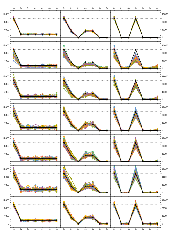
Figure 5: The three columns correspond to the three $\mathbf{x}$ vectors. The ground truth is marked by solid black lines. The bottom row is a triple Poisson tower with $m=128$, 3 cells per level. The first row is an ideal (and unrealistic) sampling-based sketch with $m^{\prime}=3\cdot 128=384$ that can magically do singleton-detection for free (the false-zeros that affect the support size estimation are also corrected for free). Rows 2,…,6 use Theorem A.1’s singleton-detector with $r=2,\ldots,6$ respectively, and $m^{\prime}=(3\cdot 128)/2r$.

We discuss a few interesting phenomena in Fig. 5.

• Observe rows 1–6. Row 1 is an unrealistic idealized sketch that gets singleton-detection for free. The errors shown in row 1 are solely due to sampling errors. As expected, there is a clear trade-off between bias and variance for the singleton-detection based estimators, rows 2–6 with $r=2,\ldots,6$. When the fingerprint width $r$ increases, the false-positive rate decreases and so the bias decreases. On the other hand, since the total space is unchanged, the sampling parameter $m^{\prime}$ decreases, and thus variance increases.

• The Fourier based estimator (bottom row) is unbiased and has smaller variance than the singleton-detection based estimators.

• Singleton-detection based estimators always return non-negative estimates of occurrences by design. On the other hand, the Fourier estimator does return negative estimates (see the estimation for $\lambda_{6}$ on $\mathbf{x}_{3}$, bottom right), which may seem strange at first sight, since occurrences are non-negative. This is a natural consequence of being an unbiased estimator of $\lambda_{6}=0$. One may trade bias for variance by reporting the biased estimate $\max\{0,\hat{\lambda}_{j}\}$.

• Note that the additive structure of the input matters. In the third column, $100\%$ of $\mathbf{x}_{3}$’s support is 3s, which causes the singleton-detector to report false positives of 6 more often than 5. A collision of two 3s will look like a 6 (mod 7) with probability $2^{-r}$, whereas it takes a collision of four 3s to look like a 5 (mod 7), which occurs with probability $2^{-3r}$.

  In general, one should expect the variance at each value to be related to the group structure of the input. If all the values are in a subgroup, then all the cells in the tower are also in the subgroup. Both sampling-based and Fourier based methods will only have non-zero estimates within that subgroup.

(a) Singleton-based with oracles

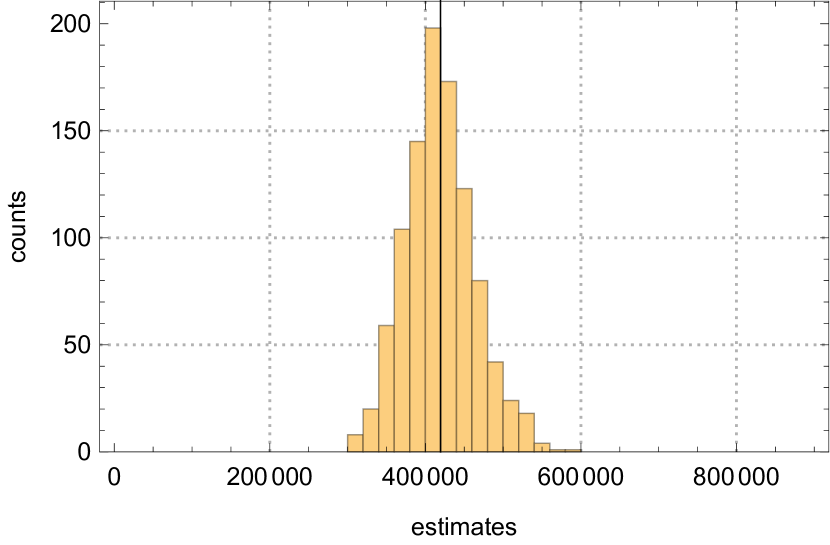
(b) Fourier-based

Figure 6: Histograms of 1000 sample runs of estimation of the $L_{2}$-moments over $\mathbb{Z}_{128}$. The corresponding $f:\mathbb{Z}_{128}\to\mathbb{C}$ is defined as $f(x)=x^{2}$, where $\mathbb{Z}_{128}$ is identified by $\{-63,\ldots,0,\ldots,64\}\subset\mathbb{Z}$. See Fig. 7 for a visualization of this function. The solid vertical line marks the correct answer. The singleton-based estimation uses $m=768$ with both empty-oracle and singleton-oracle. The Fourier-based estimation (Theorem 4.5) uses $m=256$ since it has three cells per level (note that $256\times 3=768$).

Figure 7: $x^{2}$ over $\mathbb{Z}_{128}$ corresponds to a periodic function over reals.

8.2 Unbounded Functions

Both the sampling framework and Fourier framework are still applicable when $\|f\|_{\infty}$ is large or unbounded, which degrades the variance guarantee. We find that for a toy $L_{2}$ estimation problem with $f(x)=x^{2}$, the Fourier estimator is substantially better than the sampling framework, and outperforms the pessimistic guarantee of Theorem 1.2.

Consider an input vector consisting of many small values and a few large ones:

$$\mathbf{x}=(\underbrace{1,\ldots,1}_{9900},\underbrace{64,\ldots,64}_{100}).$$

The one hundred 64s contribute $97.64\%$ of the $L_{2}$-mass while only taking $1\%$ of the $L_{0}$-mass. The singleton-detection-based scheme has high variance as the number of sampled 64s is highly variable. On the other hand, the Fourier-based scheme behaves more robustly. See Fig. 6 for a side-by-side comparison.

9 Conclusion

We introduced a general and versatile estimation framework based on Fourier transforms over any locally compact abelian group. Relational queries involving multiple streams can be answered by estimating the $f$-moment over a product group, for suitable $f$. The estimators resulting from this framework are practically superior, see Section 8.

Though the new framework shaves at most an $O(\log m+\log\log n)$ factor in terms of space complexity, we do consider this to be a major conceptual contribution to data sketches. Generic $f$-moment estimation methods developed so far in the invertible model heavily rely on evaluating the function $f$ on samples over the support, e.g., unweighted samples discussed in Section 1 or heavy-hitters in e.g., [7]. The Fourier framework attacks the problem in the dual direction: It relies on estimating the harmonic components of the $f$-moment over the whole support. The advantage of the latter is that one does not need auxiliary data structures to detect singletons/heavy hitters. We believe this work is just the starting point of the investigation of this dual direction, which will be further optimized, simplified, and generalized to other streaming estimation problems.

Appendix A Singleton-Detection over $\mathbb{G}$

0	3	3	0	0	0
3	0	0	3	3	3

(a) Likely to be a singleton with value 3.

0	3	5	0	2	2
5	2	0	5	3	3

(b) Collision happens for sure.

Figure 8: Bi-splitters, a $\mathbb{G}$-version of the singleton-detector of Ganguly, Garofalakis, and Rastogi [26]. Every value is added to exactly one slot per column. This data structure cannot handle even-ordered groups. To see this, note that if $\mathbb{G}=\mathbb{Z}_{2}$, any odd-sized collision looks like a singleton- a 1 and a 0 in every column. Thus for even-sized groups, we need to consider tri-splitters, i.e., using three rows.

Theorem A.1.

Let the set of indices hashed to $\operatorname{DetectionBucket}[k]$ be ${\mathcal{I}}_{k}^{\prime}=\mathcal{I}_{k}\cap\operatorname{supp}(\mathbf{x})$. There is $H$ such that $\operatorname{DetectionBucket}[k]$ can be interpreted with the following guarantees. If $|\mathcal{I}_{k}^{\prime}|=1$, it reports $\mathtt{singleton}$ with probability 1, as well as its $\mathbb{G}$-value. If $|\mathcal{I}_{k}^{\prime}|\neq 1$, it reports $\mathtt{not}\text{-}\mathtt{singleton}$ with probability at least $1-2^{-\Omega(r)}$ and falsely reports $\mathtt{singleton}$ with an arbitrary $\mathbb{G}$-value with probability at most $2^{-\Omega(r)}$. More precisely:

• When $|\mathbb{G}|$ is odd, there is $H:[n]\times\mathbb{G}\to\mathbb{G}^{2r}$ such that the false-positive probability is at most $(3/4)^{r}$.

• When $|\mathbb{G}|$ is even, there is $H:[n]\times\mathbb{G}\to\mathbb{G}^{3r}$ such that the false-positive probability is at most $(8/9)^{r}$.

Proof.

The scheme is visualized in Fig. 8. We analyze a single column since the columns are i.i.d. copies of each other. Let $S$ be a set sampled from $\operatorname{supp}(x)$ with an unknown size. Let $H_{b}:[n]\to\{0,1\}$ be a random partition of the universe $[n]$. A bi-splitter of $S$ is a pair $w=(\sum_{v\in S}\mathbbm{1}\left[{H_{b}(v)=0}\right]\mathbf{x}(v),\sum_{v\in S}\mathbbm{1}\left[{H_{b}(v)=1}\right]\mathbf{x}(v))$. Note that if $|S|=0$ then $w=(0,0)$. If $S=\{v\}$, $w$ is $(\mathbf{x}(v),0)$ or $(0,\mathbf{x}(v))$ with equal probabilities. For any $x\in\mathbb{G}$ with $x\neq 0$, the bi-splitter reports singleton with value $x$ if and only if $w=(x,0)$ or $w=(0,x)$. It is clear that if $S=\{v\}$ is indeed a singleton, the bi-splitter will report singleton with the correct value $\mathbf{x}(v)$ with certainty. On the other hand, when $|S|\geq 2$, the bi-splitter may falsely report singleton since non-zero values can accidentally add up to zero in groups. We now bound the false-positive probability.

Lemma A.2.

Let $\mathbb{G}$ be an odd-ordered finite abelian group. Let $x,y\in\mathbb{G}$ and $a,b\in\mathbb{G}\setminus\{0\}$. Consider the four pairs $w_{1}=(x+a+b,y),w_{2}=(x+a,y+b),w_{3}=(x+b,y+a),w_{4}=(x,y+a+b)$. Then there exists $j\in\{1,2,3,4\}$ such that $w_{j}$ does not report $\mathtt{singleton}$.

Proof.

We prove this by contradiction. Assume all $w_{j}$s report singleton.

• If $y=0$, then for $w_{2},w_{3}$ to report singleton, we need $x+b=x+a=0$, since $a,b\neq 0$. This implies $a=b=-x$. Thus we have $w_{1}=(-x,0),w_{2}=(0,-x),w_{3}=(0,-x),w_{4}=(x,-x-x)$. For $w_{4}$ to report singleton, we need exactly one of $x$ and $-x-x$ to be non-zero. Therefore, we must have $x\neq 0$ and $x+x=0$.

• If $y\neq 0$, then for $w_{1}$ to report singleton, we must have $x+a+b=0$. Thus we have $w_{1}=(0,y),w_{2}=(-b,y+b),w_{3}=(-a,y+a),w_{4}=(-a-b,y+a+b)$. However, since $a,b\neq 0$, for $w_{2},w_{3}$ to report singleton, we must have $y+b=y+a=0$, which implies $a=b=-y$. Inserting back and we have $w_{1}=(0,y),w_{2}=(y,0),w_{3}=(y,0),w_{4}=(-y-y,-y)$. Thus we must have $y+y=0$.

Thus necessarily there is an element $z\neq 0$ but $z+z=0$. However, this means $\{0,z\}$ is a subgroup of $\mathbb{G}$ and by Lagrange’s theorem we must have 2 divides $|\mathbb{G}|$. This contradicts the assumption that $\mathbb{G}$ is odd-ordered. ∎

The lemma leads to the following bound.

Corollary 2.

For any odd-ordered abelian group $\mathbb{G}$, if $|S|\geq 2$, the bi-splitter reports $\mathtt{singleton}$ with probability at most $3/4$.

Proof.

Since $|S|\geq 2$, pick any $\{u,v\}\in S$ and let $S^{\prime}=S\setminus\{u,v\}$. Let $(x,y)$ be the bi-splitter of $S^{\prime}$ and $\mathbf{x}(u)=a$, $\mathbf{x}(u)=b$. Then the bi-splitter of $S$ is $(x+a+b,y),(x+a,y+b),(x+b,y+a),(x,y+a+b)$ with equal probabilities. By Lemma A.2, at least one of the four will not report singleton. Thus the probaility that it reports singleton is at most 3/4. ∎

To handle even-ordered abelian groups, we may use a tri-splitter. Let $H_{t}:[n]\to\{0,1,2\}$ and the tri-splitter is a tuple $w=(\sum_{v\in S}\mathbbm{1}\left[{H_{t}(v)=0}\right]\mathbf{x}(v),\sum_{v\in S}\mathbbm{1}\left[{H_{t}(v)=1}\right]\mathbf{x}(v),\sum_{v\in S}\mathbbm{1}\left[{H_{t}(v)=2}\right]\mathbf{x}(v))$. A tri-splitter $w$ will report singleton with a nonzero value $x$ if and only if $w$ is $(x,0,0)$, $(0,x,0)$, or $(0,0,x)$.

Lemma A.3.

Let $\mathbb{G}$ be any finite abelian group. Let $x,y,z\in\mathbb{G}$ and $a,b\in\mathbb{G}\setminus\{0\}$. Consider the five tuples $w_{1}=(x+a,y+b,z),w_{2}=(x+b,y+a,z),w_{3}=(x,y,z+a+b),w_{4}=(x,y+a,z+b),w_{5}=(x+a,y,z+b)$. Then there exists $j\in\{1,2,3,4,5\}$ such that $w_{j}$ does not report $\mathtt{singleton}$.

Proof.

We prove this by contradiction. Assume all $w_{j}$s report singleton.

• If $z\neq 0$, then for $w_{1},w_{2}$ to report singleton, we must have $x=y=-a=-b\neq 0$. However, this implies $w_{3}=(-a,-b,z+a+b)$ where $a,b\neq 0$. Contradiction.

• If $z=0$, then for $w_{4}$ to report singleton, we need have $x=0$ and $y=-a$. But this implies $w_{5}=(a,-a,b)$ where $a,b\neq 0$. Contradiction.

∎

Corollary 3.

For any even-ordered abelian group $\mathbb{G}$, if $|S|\geq 2$, the tri-splitter reports $\mathtt{singleton}$ with probability at most $8/9$.

Proof.

Similar to the proof of Corollary 2. ∎

Finally we conclude the proof by noting that both splitters can be repeated $r$ times independently to reduce the bounds of false-positive probability to $(3/4)^{r}$ and $(8/9)^{r}$. ∎

Appendix B Mathematical Lemmas

Lemma B.1.

Let $h:\mathbb{R}\to\mathbb{C}$ be a differentiable function. If both $h$ and $h^{\prime}$ are (Lebesgure) integrable, then

$$\left|\int_{-\infty}^{\infty}h(s)\,ds-\frac{1}{m}\sum_{k=-\infty}^{\infty}h(k/m)\right|\leq m^{-1}\int_{-\infty}^{\infty}|h^{\prime}(s)|\,ds.$$

Proof.

We bound the difference

$$\left|\int_{-\infty}^{\infty}h(s)\,ds-\frac{1}{m}\sum_{k=-\infty}^{\infty}h(k/m)\right| =\left|\sum_{k=-\infty}^{\infty}\left(\int_{0}^{1/m}h(k/m+s)\,ds-\frac{1}{m}h(k/m)\right)\right|$$

$$\leq\sum_{k=-\infty}^{\infty}\left|\int_{0}^{1/m}h(k/m+s)\,ds-\frac{1}{m}h(k/m)\right|.$$

Note that

$$\left|\int_{0}^{1/m}h(k/m+s)\,ds-\frac{1}{m}h(k/m)\right| =\left|\int_{0}^{1/m}\int_{0}^{s}h^{\prime}(k/m+t)\,dtds\right|$$

$$\leq\int_{0}^{1/m}\int_{0}^{s}|h^{\prime}(k/m+t)|\,dtds$$

$$\leq\int_{0}^{1/m}\int_{0}^{1/m}|h^{\prime}(k/m+t)|\,dtds$$

$$=\frac{1}{m}\int_{0}^{1/m}|h^{\prime}(k/m+t)|\,dt.$$

Thus

$$\left|\int_{-\infty}^{\infty}h(s)\,ds-\frac{1}{m}\sum_{j=-\infty}^{\infty}h(j/m)\right| \leq\sum_{k=-\infty}^{\infty}\frac{1}{m}\int_{0}^{1/m}|h^{\prime}(k/m+t)|\,dt$$

$$=\frac{1}{m}\int_{-\infty}^{\infty}|h^{\prime}(t)|\,dt.$$

∎

Lemma B.2.

Let $a,b\in\mathbb{C}$ and $c\in\mathbb{R}$. Define

$$\eta_{1}(x;a,b,c) =(e^{-ae^{-x}}-e^{-be^{-x}})e^{cx}, \eta_{2}(x;a,c) =ae^{-x}e^{-ae^{-x}}e^{cx}.$$

If $\mathfrak{Re}(a)\geq 0$, $\mathfrak{Re}(b)\geq 0$ and $c\in(0,1)$, then

1. $\int_{-\infty}^{\infty}\eta_{1}(x;a,b,c)\,dx=(a^{c}-b^{c})\Gamma(-c),$ where $\Gamma(\cdot)$ here denotes the Gamma function (Fig. 2);

2. $\eta_{1}^{\prime}(x;a,b,c)=c\eta_{1}(x;a,b,c)+\eta_{2}(x;a,c)-\eta_{2}(x;b,c)$;

3. $\int_{-\infty}^{\infty}|\eta_{1}(x;a,b,c)|\,dx\leq 2\left(\frac{1}{c}+\frac{1}{1-c}\right)|b-a|^{c}$.

4. $\int_{-\infty}^{\infty}|\eta_{2}(x;a,c)|\,dx\leq|a|^{c}\Gamma(1-c)$.

5. $\int_{-\infty}^{\infty}|\eta_{1}^{\prime}(x;a,b,c)|\,dx\leq 2\left(1+\frac{c}{1-c}\right)|b-a|^{c}+(|a|^{c}+|b|^{c})\Gamma(1-c)$.

6. $$\left|\int_{-\infty}^{\infty}\eta_{1}(x;a,b,c)\,dx-\frac{1}{m}\sum_{k=-\infty}^{\infty}\eta_{1}(k/m;a,b,c)\right|$$

   $${\hskip 113.81102pt}\leq m^{-1}\left(2\left(1+\frac{c}{1-c}\right)|b-a|^{c}+(|a|^{c}+|b|^{c})\Gamma(1-c)\right).$$

Proof.

Part 1. Integral by parts.

$$\int_{-\infty}^{\infty}(e^{-ae^{-x}}-e^{-be^{-x}})e^{cx}\,dx$$

$$=\left.(e^{-ae^{-x}}-e^{-be^{-x}})c^{-1}e^{cx}\right|_{-\infty}^{\infty}-\int_{-\infty}^{\infty}(ae^{-x}e^{-ae^{-x}}-be^{-x}e^{-be^{-x}})c^{-1}e^{cx}\,dx$$

Since $$\mathfrak{Re}(a)\geq 0 \mathfrak{Re}(b)\geq 0 c\in(0,1) \left.(e^{-ae^{-x}}-e^{-be^{-x}})c^{-1}e^{cx}\right|_{-\infty}^{\infty}=0$$, and , ,

$$=-c^{-1}\int_{-\infty}^{\infty}ae^{-(1-c)x}e^{-ae^{-x}}\,dx+c^{-1}\int_{-\infty}^{\infty}be^{-(1-c)x}e^{-be^{-x}}\,dx.$$

Set $z=ae^{-x}$ and we have

$$c^{-1}\int_{-\infty}^{\infty}ae^{-(1-c)x}e^{-ae^{-x}}\,dx =c^{-1}\int_{0}^{\infty}a^{c}z^{-c}e^{-z}\,dz$$

$$=a^{c}\frac{\Gamma(1-c)}{c}=a^{c}(-\Gamma(-c)).$$ (8)

Thus

$$\int_{-\infty}^{\infty}(e^{-ae^{-x}}-e^{-be^{-x}})e^{cx}\,dx =-a^{c}(-\Gamma(-c))+b^{c}(-\Gamma(-c))=(a^{c}-b^{c})\Gamma(-c).$$

Part 2.

$$\eta_{1}^{\prime}(x;a,b,c) =(e^{-ae^{-x}}-e^{-be^{-x}})ce^{cx}+(ae^{-x}e^{-ae^{-x}}-be^{-x}e^{-be^{-x}})e^{cx}$$

$$=c\eta_{1}(x;a,b,c)+\eta_{2}(x;a,c)-\eta_{2}(x;b,c).$$

Part 3. Define the path $\phi(t)=(1-t)a+tb$ and $g_{x}(r)=e^{-re^{-x}}$. By the path integral,

$$\left|e^{-ae^{-x}}-e^{-be^{-x}}\right| =|g_{x}(a)-g_{x}(b)|=\left|\int_{0}^{1}g_{x}^{\prime}(\phi(t))\phi^{\prime}(t)\,dt\right|$$

$$=\left|\int_{0}^{1}e^{-\phi(t)e^{-x}}(-e^{-x})(b-a)\,dt\right|\leq|b-a|e^{-x}\int_{0}^{1}|e^{-\phi(t)e^{-x}}|\,dt$$

We assumed $$\mathfrak{Re}(a),\mathfrak{Re}(b)\geq 0 \mathfrak{Re}(\phi(t))\geq 0 t\in[0,1] |e^{-\phi(t)e^{-x}}|<1$$ and thus for any , which implies . We then have

$$\left|e^{-ae^{-x}}-e^{-be^{-x}}\right| \leq|b-a|e^{-x}.$$

On the other hand, since $\mathfrak{Re}(a),\mathfrak{Re}(b)\geq 0$, we have $\left|e^{-ae^{-x}}\right|,\left|e^{-be^{-x}}\right|\leq 1$ and thus

$$\left|e^{-ae^{-x}}-e^{-be^{-x}}\right| \leq\left|e^{-ae^{-x}}\right|+\left|e^{-ae^{-x}}\right|\leq 2.$$

We conclude that for any $q\in\mathbb{R}$

$$\int_{-\infty}^{\infty}\left|(e^{-ae^{-x}}-e^{-be^{-x}})e^{cx}\right|\,dx =\int_{-\infty}^{q}\left|e^{-ae^{-x}}-e^{-be^{-x}}\right|e^{cx}\,dx+\int_{q}^{\infty}\left|e^{-ae^{-x}}-e^{-be^{-x}}\right|e^{cx}\,dx$$

$$\leq\int_{-\infty}^{q}2e^{cx}\,dx+\int_{q}^{\infty}|b-a|e^{-x}e^{cx}\,dx$$

$$=2\frac{e^{cq}}{c}+|b-a|\frac{e^{(c-1)q}}{1-c},$$

since $$c\in(0,1) q=\log|b-a|$$. Now set and we have

$$\int_{-\infty}^{\infty}\left|(e^{-ae^{-x}}-e^{-be^{-x}})e^{cx}\right|\,dx \leq 2\left(\frac{1}{c}+\frac{1}{1-c}\right)|b-a|^{c}.$$

Part 4.

$$\int_{-\infty}^{\infty}\left|ae^{-x}e^{-ae^{-x}}e^{cx}\right|\,dx =|a|\int_{-\infty}^{\infty}e^{-x}e^{-\mathfrak{Re}({a})e^{-x}}e^{cx}\,dx$$

by Eq. 8, since $$\mathfrak{Re}({a})\geq 0$$

$$=|a|\frac{1}{\mathfrak{Re}(a)}(\mathfrak{Re}(a))^{c}\Gamma(1-c)$$

$$\leq|a|^{c}\Gamma(1-c).$$

Part 5. Follows from 2, 3, and 4.

Part 6. Follows from 5 and Lemma B.1. ∎

Appendix C Proof of Theorem 6.1 — Truncated Poisson Tower Sketch

Let us recall Theorem 6.1.

See 6.1

We first prove two technical lemmas. Fix $a,b\in\mathbb{R}$, $m\geq 2$.

Lemma C.1.

Define $\tau_{1},\tau_{2},\tau_{3}$ as

• $\tau_{1}=16m\lambda^{1/3}$,

• $\tau_{2}=e^{\frac{1}{3}(a-1)/m}\frac{1}{1-e^{-1/(3m)}}$,

• $\tau_{3}=4m\lambda e^{-\frac{2}{3}b/m}$.

Then for any $\gamma\in\mathbbold{\Gamma}$,

1. $\mathbb{E}\sum_{k=-\infty}^{\infty}|{\boldsymbol{(}{X_{k}},{\gamma}\boldsymbol{)}}-1|e^{\frac{1}{3}k/m}\leq\tau_{1}$.

2. $\sum_{k=-\infty}^{a-1}|{\boldsymbol{(}{X_{k}},{\gamma}\boldsymbol{)}}|e^{\frac{1}{3}k/m}=\tau_{2}\leq 4me^{\frac{1}{3}(a-1)/m}$.

3. $\mathbb{E}\sum_{k=b}^{\infty}|{\boldsymbol{(}{X_{k}},{\gamma}\boldsymbol{)}}-1|e^{\frac{1}{3}k/m}\leq\tau_{3}$.

Proof.

Part 1. Note that $|{\boldsymbol{(}{X_{k}},{\gamma}\boldsymbol{)}}-1|\leq 2$ and $|{\boldsymbol{(}{X_{k}},{\gamma}\boldsymbol{)}}-1|=0$ if $X_{k}=0$.

$$\mathbb{E}\sum_{k=-\infty}^{\infty}|{\boldsymbol{(}{X_{k}},{\gamma}\boldsymbol{)}}-1|e^{\frac{1}{3}k/m}$$

$$\leq\mathbb{E}\sum_{k=-\infty}^{\infty}2\cdot\mathbbm{1}\left[{X_{k}\neq 0}\right]e^{\frac{1}{3}k/m}$$

Since the $$\{X_{k}\} \mathbb{P}(X_{k}\neq 0)=1-e^{-\lambda e^{-k/m}}$$ are independent and ,

$$\leq\sum_{k=-\infty}^{\infty}2\cdot(1-e^{-\lambda e^{-k/m}})e^{\frac{1}{3}k/m}$$

$$=2\sum_{k=-\infty}^{\infty}\eta_{1}(k/m;a,b,c)$$

where $$a=0,b=\lambda,c=1/3$$. By Lemma B.2(6),

$$\leq 2m\int_{-\infty}^{\infty}\eta_{1}(x;a,b,c)\,dx+2\left|m\int_{-\infty}^{\infty}\eta_{1}(x;a,b,c)\,dx-\sum_{k=-\infty}^{\infty}\eta_{1}(k/m;a,b,c)\right|$$

$$=2m(a^{c}-b^{c})\Gamma(-c)+2\left(2\left(1+\frac{c}{1-c}\right)|b-a|^{c}+(|a|^{c}+|b|^{c})\Gamma(1-c)\right)$$

$$=2m\lambda^{1/3}(-\Gamma(-1/3))+2\lambda^{1/3}(3+\Gamma(2/3))$$

when $$m\geq 2$$,

$$\leq 16m\lambda^{1/3}=\tau_{1}.$$

Part 2. Remember that for all $\gamma$, $|{\boldsymbol{(}{X_{k}},{\gamma}\boldsymbol{)}}|=1$.

$$\sum_{k=-\infty}^{a-1}|{\boldsymbol{(}{X_{k}},{\gamma}\boldsymbol{)}}|e^{\frac{1}{3}k/m} =\sum_{k=-\infty}^{a-1}e^{\frac{1}{3}k/m}=e^{\frac{1}{3}(a-1)/m}\frac{1}{1-e^{-1/(3m)}}=\tau_{2}\leq 4me^{\frac{1}{3}(a-1)/m}.$$

The last inequality follows from $e^{-1/(3m)}\leq 1-\frac{1}{4m}$, which holds when $m\geq 2$.

Part 3. Observe that $|{\boldsymbol{(}{X_{k}},{\gamma}\boldsymbol{)}}-1|\leq 2$ and $|{\boldsymbol{(}{X_{k}},{\gamma}\boldsymbol{)}}-1|=0$ if $X_{k}=0$.

$$\mathbb{E}\sum_{k=b}^{\infty}|{\boldsymbol{(}{X_{k}},{\gamma}\boldsymbol{)}}-1|e^{\frac{1}{3}k/m} \leq\mathbb{E}\sum_{k=b}^{\infty}2\cdot\mathbbm{1}\left[{X_{k}\neq 0}\right]e^{\frac{1}{3}k/m}$$

Since the $$\{X_{k}\} \mathbb{P}(X_{k}\neq 0)=1-e^{-\lambda e^{-k/m}}$$ are independent and ,

$$\leq\sum_{k=b}^{\infty}2\cdot(1-e^{-\lambda e^{-k/m}})e^{\frac{1}{3}k/m}$$

Note that $$e^{-\lambda e^{-k/m}}\geq 1-\lambda e^{-k/m}$$. Continuing,

$$\leq 2\sum_{k=b}^{\infty}\lambda e^{-k/m}e^{\frac{1}{3}k/m}$$

$$=2\lambda e^{-\frac{2}{3}b/m}\frac{1}{1-e^{-2/(3m)}}\;\leq\;4m\lambda e^{-\frac{2}{3}b/m}\;=\;\tau_{3}.$$

The last inequality follows from $e^{-2/(3m)}\leq 1-\frac{1}{2m}$ when $m\geq 2$. ∎

Lemma C.2.

For $\gamma\in\mathbbold{\Gamma}$, define $A_{\gamma},B_{\gamma}$, and $C_{\gamma}$ as:

$$A_{\gamma} =U_{\gamma}, B_{\gamma} =U_{\gamma;-\infty,a}+\tau_{2}, C_{\gamma} =U_{\gamma;b,\infty}.$$

The following statements are true. For any $\gamma,\gamma^{\prime}\in\mathbbold{\Gamma}$,

1. $\mathbb{E}|A_{\gamma}|\leq\tau_{1}$.

2. $|B_{\gamma}|\leq\tau_{2}$.

3. $\mathbb{E}|C_{\gamma}|\leq\tau_{3}$.

4. $\mathbb{E}|A_{\gamma}||B_{\gamma^{\prime}}|\leq\tau_{1}\tau_{2}$.

5. $\mathbb{E}|B_{\gamma}||C_{\gamma^{\prime}}|\leq\tau_{2}\tau_{3}$.

6. $|B_{\gamma}||B_{\gamma^{\prime}}|\leq\tau_{2}^{2}$.

7. $\mathbb{E}|C_{\gamma}||C_{\gamma^{\prime}}|\leq\tau_{3}^{2}+16m\lambda e^{-\frac{1}{3}b/m}$.

8. $\mathbb{E}|A_{\gamma}||C_{\gamma^{\prime}}|\leq\tau_{1}\tau_{3}+16m\lambda e^{-\frac{1}{3}b/m}$.

9. $\mathbb{E}|A_{\gamma}||A_{\gamma^{\prime}}|\leq\tau_{1}^{2}+36m\lambda^{2/3}$.

Proof.

Part 1. By Lemma C.1(1),

$$\mathbb{E}|A_{\gamma}|=\mathbb{E}|U_{\gamma}| \leq\mathbb{E}\sum_{k=-\infty}^{\infty}|{\boldsymbol{(}{X_{k}},{\gamma}\boldsymbol{)}}-1|e^{\frac{1}{3}k/m}\leq\tau_{1}.$$

Part 2. Note that $\sum_{k=-\infty}^{a-1}e^{\frac{1}{3}k/m}=e^{\frac{1}{3}(a-1)/m}\frac{1}{1-e^{-1/(3m)}}.$ By Lemma C.1(2),

$$\left|U_{\gamma;-\infty,a}+e^{\frac{1}{3}(a-1)/m}\frac{1}{1-e^{-1/(3m)}}\right| =\left|\sum_{k=-\infty}^{a-1}({\boldsymbol{(}{X_{k}},{\gamma}\boldsymbol{)}}-1)e^{\frac{1}{3}k/m}+\sum_{k=-\infty}^{a-1}e^{\frac{1}{3}k/m}\right|$$

$$=\left|\sum_{k=-\infty}^{a-1}{\boldsymbol{(}{X_{k}},{\gamma}\boldsymbol{)}}e^{\frac{1}{3}k/m}\right|\leq\tau_{2}.$$

Part 3. By Lemma C.1(3),

$$\mathbb{E}|U_{\gamma;b,\infty}| \leq\mathbb{E}\sum_{k=b}^{\infty}|{\boldsymbol{(}{X_{k}},{\gamma}\boldsymbol{)}}-1|e^{\frac{1}{3}k/m}\leq\tau_{3}.$$

Part 4. Follows from parts 1 and 2.

Part 5. Follows from parts 2 and 3.

Part 6. Follows from part 2.

Part 7. Recall that $X_{j},X_{k}$ are independent for $j\neq k$.

$$\mathbb{E}|C_{\gamma}||C_{\gamma^{\prime}}|=\mathbb{E}|U_{\gamma;b,\infty}U_{\gamma^{\prime};b,\infty}| =\mathbb{E}\left|\sum_{k=b}^{\infty}\sum_{j=b}^{\infty}({\boldsymbol{(}{X_{k}},{\gamma}\boldsymbol{)}}-1)({\boldsymbol{(}{X_{j}},{\gamma^{\prime}}\boldsymbol{)}}-1)e^{\frac{k+j}{3m}}\right|$$

$$\leq\sum_{k=b}^{\infty}\sum_{j=b}^{\infty}\mathbb{E}\left|({\boldsymbol{(}{X_{k}},{\gamma}\boldsymbol{)}}-1)({\boldsymbol{(}{X_{j}},{\gamma^{\prime}}\boldsymbol{)}}-1)\right|e^{\frac{k+j}{3m}}$$

$$\leq\tau_{3}^{2}+\sum_{k=b}^{\infty}\mathbb{E}\left|({\boldsymbol{(}{X_{k}},{\gamma}\boldsymbol{)}}-1)({\boldsymbol{(}{X_{k}},{\gamma^{\prime}}\boldsymbol{)}}-1)\right|e^{\frac{2k}{3m}},$$

where by Lemma C.1(3) we know $\tau_{3}$ upper bounds $\mathbb{E}\sum_{k=b}^{\infty}|{\boldsymbol{(}{X_{k}},{\gamma}\boldsymbol{)}}-1|e^{\frac{1}{3}k/m}$. Note that $|{\boldsymbol{(}{X_{k}},{\gamma}\boldsymbol{)}}-1|\leq 2$ and $|{\boldsymbol{(}{X_{k}},{\gamma}\boldsymbol{)}}-1|=0$ if $X_{k}=0$. We also have

$$\sum_{k=b}^{\infty}\mathbb{E}\left|({\boldsymbol{(}{X_{k}},{\gamma}\boldsymbol{)}}-1)({\boldsymbol{(}{X_{k}},{\gamma^{\prime}}\boldsymbol{)}}-1)\right|e^{\frac{2k}{3m}} \leq 4\sum_{k=b}^{\infty}\mathbbm{1}\left[{X_{k}\neq 0}\right]e^{\frac{2k}{3m}}$$

$$=4\sum_{k=b}^{\infty}(1-e^{-\lambda e^{-k/m}})e^{\frac{2}{3}k/m}$$

$$\leq 4\sum_{k=b}^{\infty}\lambda e^{-k/m}\cdot e^{\frac{2}{3}k/m}$$

$$=4\lambda e^{-\frac{1}{3}b/m}\frac{1}{1-e^{-1/(3m)}}\;\leq\;16m\lambda e^{-\frac{1}{3}b/m}.$$

The last inequality follows from $e^{-1/(3m)}\leq 1-\frac{1}{4m}$ which holds when $m\geq 2$. We conclude that

$$\mathbb{E}|U_{\gamma;b,\infty}U_{\gamma^{\prime};b,\infty}| \leq\tau_{3}^{2}+16m\lambda e^{-\frac{1}{3}b/m}.$$

Part 8. Applying parts 1 and 3, we have

$$\mathbb{E}|A\gamma||C_{\gamma^{\prime}}|=\mathbb{E}|U_{\gamma}U_{\gamma^{\prime};b,\infty}| =\mathbb{E}\left|\sum_{k=-\infty}^{\infty}\sum_{j=b}^{\infty}({\boldsymbol{(}{X_{k}},{\gamma}\boldsymbol{)}}-1)({\boldsymbol{(}{X_{j}},{\gamma^{\prime}}\boldsymbol{)}}-1)e^{\frac{k+j}{3m}}\right|$$

$$\leq\sum_{k=-\infty}^{\infty}\sum_{j=b}^{\infty}\mathbb{E}\left|({\boldsymbol{(}{X_{k}},{\gamma}\boldsymbol{)}}-1)({\boldsymbol{(}{X_{j}},{\gamma^{\prime}}\boldsymbol{)}}-1)\right|e^{\frac{k+j}{3m}}$$

$$\leq\tau_{1}\tau_{3}+\sum_{k=b}^{\infty}\mathbb{E}\left|({\boldsymbol{(}{X_{k}},{\gamma}\boldsymbol{)}}-1)({\boldsymbol{(}{X_{k}},{\gamma^{\prime}}\boldsymbol{)}}-1)\right|e^{\frac{2k}{3m}},$$

where by Lemma C.1 we know $$\tau_{1} \mathbb{E}\sum_{k=-\infty}^{\infty}|{\boldsymbol{(}{X_{k}},{\gamma}\boldsymbol{)}}-1|e^{\frac{1}{3}k/m} \tau_{3} \mathbb{E}\sum_{k=b}^{\infty}|{\boldsymbol{(}{X_{k}},{\gamma}\boldsymbol{)}}-1|e^{\frac{1}{3}k/m}$$ upper bounds and upper bounds . From the proof of part 7, we know this is

$$\leq\tau_{1}\tau_{3}+16m\lambda e^{-\frac{1}{3}b/m}.$$

Part 9. Applying part 1,

$$\mathbb{E}|A_{\gamma}||A_{\gamma^{\prime}}|=\mathbb{E}|U_{\gamma}U_{\gamma^{\prime}}| =\mathbb{E}\left|\sum_{k=-\infty}^{\infty}\sum_{j=-\infty}^{\infty}({\boldsymbol{(}{X_{k}},{\gamma}\boldsymbol{)}}-1)({\boldsymbol{(}{X_{j}},{\gamma^{\prime}}\boldsymbol{)}}-1)e^{\frac{k+j}{3m}}\right|$$

$$\leq\sum_{k=-\infty}^{\infty}\sum_{j=-\infty}^{\infty}\mathbb{E}\left|({\boldsymbol{(}{X_{k}},{\gamma}\boldsymbol{)}}-1)({\boldsymbol{(}{X_{j}},{\gamma^{\prime}}\boldsymbol{)}}-1)\right|e^{\frac{k+j}{3m}}$$

$$\leq\tau_{1}^{2}+\sum_{k=-\infty}^{\infty}\mathbb{E}\left|({\boldsymbol{(}{X_{k}},{\gamma}\boldsymbol{)}}-1)({\boldsymbol{(}{X_{k}},{\gamma^{\prime}}\boldsymbol{)}}-1)\right|e^{\frac{2k}{3m}}$$

where by Lemma C.1 we know $$\tau_{1} \mathbb{E}\sum_{k=-\infty}^{\infty}|{\boldsymbol{(}{X_{k}},{\gamma}\boldsymbol{)}}-1|e^{\frac{1}{3}k/m}$$ upper bounds .

$$\leq\tau_{1}^{2}+2\sum_{k=-\infty}^{\infty}\mathbb{E}\left|({\boldsymbol{(}{X_{k}},{\gamma^{\prime}}\boldsymbol{)}}-1)\right|e^{\frac{2k}{3m}}.$$

Similar to the proof of Lemma C.1(1), we have

$$\mathbb{E}\sum_{k=-\infty}^{\infty}|{\boldsymbol{(}{X_{k}},{\gamma}\boldsymbol{)}}-1|e^{\frac{2}{3}k/m}$$

$$\leq 2m(a^{c}-b^{c})\Gamma(-c)+2\left(2\left(1+\frac{c}{1-c}\right)|b-a|^{c}+(|a|^{c}+|b|^{c})\Gamma(1-c)\right)$$

where $$a=0,b=\lambda,c=2/3$$

$$=2m\lambda^{2/3}(-\Gamma(-2/3))+2\lambda^{2/3}(6+\Gamma(1/3))\;\leq\;18m\lambda^{2/3}.$$

Where the last inequality holds when $m\geq 2$. We conclude that $\mathbb{E}|U_{\gamma}U_{\gamma^{\prime}}|\leq\tau_{1}^{2}+36m\lambda^{2/3}$. ∎

We are now in a position to prove Theorem 6.1.

Proof of Theorem 6.1.

Part 1: bias. Note that $U_{\gamma}=A_{\gamma}$ and $U_{\gamma;a,b}-\tau_{2}=A_{\gamma}-B_{\gamma}-C_{\gamma}$.

$$|\mathbb{E}\phi_{f,m}(X)-\mathbb{E}\phi_{f,m;a,b}(X)| \leq\mathbb{E}|\phi_{f,m}(X)-\phi_{f,m;a,b}(X)|$$

$$=\mathbb{E}\left|\int{\Gamma}\hat{f}(\gamma)\frac{\prod_{j=1}^{3}A_{\gamma}^{(j)}-\prod_{j=1}^{3}(A_{\gamma}^{(j)}-B_{\gamma}^{(j)}-C_{\gamma}^{(j)})}{m^{3}\Gamma(-1/3)^{3}}\,d\mu_{\mathbbold{\Gamma}}(\gamma)\right|$$

$$\leq\int{\Gamma}|\hat{f}(\gamma)|\frac{\mathbb{E}\left|\prod_{j=1}^{3}A_{\gamma}^{(j)}-\prod_{j=1}^{3}(A_{\gamma}^{(j)}-B_{\gamma}^{(j)}-C_{\gamma}^{(j)})\right|}{m^{3}|\Gamma(-1/3)|^{3}}\,d\mu{\Gamma}\gamma.$$

By the independence of the three copies,

$$\mathbb{E}\left|\prod_{j=1}^{3}A_{\gamma}^{(j)}-\prod_{j=1}^{3}(A_{\gamma}^{(j)}-B_{\gamma}^{(j)}-C_{\gamma}^{(j)})\right|$$

$$\leq 3(\mathbb{E}|A_{\gamma}|)^{2}(\mathbb{E}|B_{\gamma}|+\mathbb{E}|C_{\gamma}|)+3(\mathbb{E}|A_{\gamma}|)(\mathbb{E}|B_{\gamma}|+\mathbb{E}|C_{\gamma}|)^{2}+(\mathbb{E}|B_{\gamma}|+\mathbb{E}|C_{\gamma}|)^{3}.$$

Since we assumed $a\leq m(\ln\lambda-6\ln m)$ and $b\geq m(\ln\lambda+3\ln m)$, by Lemma C.2 we have

$$\mathbb{E}|A_{\gamma}| \leq\tau_{1}=16m\lambda^{1/3},$$

$$\mathbb{E}|B_{\gamma}| \leq\tau_{2}\leq 4me^{\frac{1}{3}a/m}\leq 4m^{-1}\lambda^{1/3},$$

$$\mathbb{E}|C_{\gamma}| \leq\tau_{3}=4m\lambda e^{-\frac{2}{3}b/m}\leq 4m^{-1}\lambda^{1/3}.$$

Thus we have

$$\mathbb{E}\left|\prod_{j=1}^{3}A_{\gamma}^{(j)}-\prod_{j=1}^{3}(A_{\gamma}^{(j)}-B_{\gamma}^{(j)}-C_{\gamma}^{(j)})\right| =O(m^{2}\lambda^{2/3}\cdot m^{-1}\lambda^{1/3})=\lambda\cdot O(m).$$

We conclude that

$$|\mathbb{E}\phi_{f,m}(X)-\mathbb{E}\phi_{f,m;a,b}(X)| \leq\int{\Gamma}|\hat{f}(\gamma)|\frac{\lambda\cdot O(m)}{m^{3}|\Gamma(-1/3)|^{3}}\,d\mu{\Gamma}\gamma$$

$$=\lambda\|\hat{f}\|_{1}O(m^{-2}).$$

Part 2: variance.

$$\mathbb{E}\left|\phi_{f,m}(X)\overline{\phi_{f,m}(X)}-\phi_{f,m;a,b}(X)\overline{\phi_{f,m;a,b}(X)}\right|$$

$$\leq\mathbb{E}\left|\int{\Gamma}\int{\Gamma}\hat{f}(\gamma)\overline{\hat{f}(\gamma)}\frac{\prod_{j=1}^{3}A_{\gamma}^{(j)}\overline{A_{\gamma^{\prime}}^{(j)}}-\prod_{j=1}^{3}(A_{\gamma}^{(j)}-B_{\gamma}^{(j)}-C_{\gamma}^{(j)})\overline{(A_{\gamma^{\prime}}^{(j)}-B_{\gamma^{\prime}}^{(j)}-C_{\gamma^{\prime}}^{(j)})}}{m^{6}\Gamma(-1/3)^{6}}\,d\mu_{\mathbbold{\Gamma}}(\gamma)d\mu_{\mathbbold{\Gamma}}(\gamma^{\prime})\right|$$

$$\leq\int{\Gamma}\int{\Gamma}|\hat{f}(\gamma)||\overline{\hat{f}(\gamma)}|\frac{\mathbb{E}\left|\prod_{j=1}^{3}A_{\gamma}^{(j)}\overline{A_{\gamma^{\prime}}^{(j)}}-\prod_{j=1}^{3}(A_{\gamma}^{(j)}-B_{\gamma}^{(j)}-C_{\gamma}^{(j)})\overline{(A_{\gamma^{\prime}}^{(j)}-B_{\gamma^{\prime}}^{(j)}-C_{\gamma^{\prime}}^{(j)})}\right|}{m^{6}|\Gamma(-1/3)|^{6}}\,d\mu_{\mathbbold{\Gamma}}(\gamma)d\mu_{\mathbbold{\Gamma}}(\gamma^{\prime}),$$

We expand the product $\prod_{j=1}^{3}(A_{\gamma}^{(j)}-B_{\gamma}^{(j)}-C_{\gamma}^{(j)})\overline{(A_{\gamma^{\prime}}^{(j)}-B_{\gamma^{\prime}}^{(j)}-C_{\gamma^{\prime}}^{(j)})}$ and cancel the term $\prod_{j=1}^{3}A_{\gamma}^{(j)}\overline{A_{\gamma^{\prime}}^{(j)}}$. By the independence of the three copies, we have

$$\mathbb{E}\left|\prod_{j=1}^{3}A_{\gamma}^{(j)}\overline{A_{\gamma^{\prime}}^{(j)}}-\prod_{j=1}^{3}(A_{\gamma}^{(j)}-B_{\gamma}^{(j)}-C_{\gamma}^{(j)})\overline{(A_{\gamma^{\prime}}^{(j)}-B_{\gamma^{\prime}}^{(j)}-C_{\gamma^{\prime}}^{(j)})}\right|$$

$$\leq(z_{AA}+z_{BB}+z_{CC}+2z_{AB}+2z_{BC}+2z_{CA})^{3}-z_{AA}^{3}$$

where $z_{AA},z_{BB},z_{CC},z_{AB},z_{BC},z_{CA}$ are the upper bounds from Lemma C.2. Since we assumed $a\leq m(\ln\lambda-6\ln m)$ and $b\geq m(\ln\lambda+3\ln m)$, we have

$$\mathbb{E}|A_{\gamma}||A_{\gamma^{\prime}}| \leq z_{AA}=\tau_{1}^{2}+36m\lambda^{2/3}=\lambda^{2/3}O(m^{2}),$$

$$\mathbb{E}|B_{\gamma}||B_{\gamma^{\prime}}| \leq z_{BB}=\tau_{2}^{2}=\lambda^{2/3}O(m^{-2}),$$

$$\mathbb{E}|C_{\gamma}||C_{\gamma^{\prime}}| \leq z_{CC}=\tau_{3}^{2}+16m\lambda e^{-\frac{1}{3}b/m}=\lambda^{2/3}O(1),$$

$$\mathbb{E}|A_{\gamma}||B_{\gamma^{\prime}}| \leq z_{AB}=\tau_{1}\tau_{2}=\lambda^{2/3}O(1),$$

$$\mathbb{E}|B_{\gamma}||C_{\gamma^{\prime}}| \leq z_{BC}=\tau_{2}\tau_{3}=\lambda^{2/3}O(m^{-2}),$$

$$\mathbb{E}|C_{\gamma}||A_{\gamma^{\prime}}| \leq z_{CA}=\tau_{1}\tau_{3}+16m\lambda e^{-\frac{1}{3}b/m}=\lambda^{2/3}O(1).$$

Thus we have

$$(z_{AA}+z_{BB}+z_{CC}+2z_{AB}+2z_{BC}+2z_{CA})^{3}-z_{AA}^{3}=\lambda^{2}O(m^{4}),$$

and therefore

$$\mathbb{E}\left|\phi_{f,m}(X)\overline{\phi_{f,m}(X)}-\phi_{f,m;a,b}(X)\overline{\phi_{f,m;a,b}(X)}\right| \leq\lambda^{2}\|\hat{f}\|_{1}^{2}O(m^{-2}).$$

We conclude that

$$|\mathbb{V}(\phi_{f,m;a,b}(X))-\mathbb{V}(\phi_{f,m;}(X))| \leq\left|\mathbb{E}\phi_{f,m;a,b}(X)\overline{\phi_{f,m;a,b}(X)}-(\mathbb{E}\phi_{f,m;a,b}(X))\overline{(\mathbb{E}\phi_{f,m;a,b}(X))}\right.$$

$$\quad\quad\left.{}-\mathbb{E}\phi_{f,m}(X)\overline{\phi_{f,m}(X)}+(\mathbb{E}\phi_{f,m}(X))\overline{(\mathbb{E}\phi_{f,m}(X))}\right|$$

Note that for two complex numbers $$w_{1},w_{2} |w_{1}\overline{w_{1}}-w_{2}\overline{w_{2}}|\leq|w_{1}-w_{2}|(|w_{1}|+|w_{2}|)$$,

$$\leq\mathbb{E}\left|\phi_{f,m}(X)\overline{\phi_{f,m}(X)}-\phi_{f,m;a,b}(X)\overline{\phi_{f,m;a,b}(X)}\right|$$

$$\quad\quad{}+\mathbb{E}|\phi_{f,m}(X)-\phi_{f,m;a,b}(X)|(|\mathbb{E}\phi_{f,m}(X)|+|\mathbb{E}\phi_{f,m;a,b}(X)|)$$

$$=\lambda^{2}\|\hat{f}\|_{1}^{2}O(m^{-2})+\lambda\|\hat{f}\|_{1}O(m^{-2})(\lambda|\mathbb{E}f(R)|+\lambda\|\hat{f}\|_{1}O(m^{-1}))$$

where $$|\mathbb{E}f(R)|\leq\|f\|_{\infty} \|f\|_{\infty}\leq\|\hat{f}\|_{1}$$ and, by Lemma 2.4, . In conclusion, this is

$$=\lambda^{2}\|\hat{f}\|_{1}^{2}O(m^{-2}).\hskip 204.85974pt\qed$$

Appendix D Proof of Theorem 6.2 — Depoissonization

Let use recall Theorem 6.2.

See 6.2

In the analysis of truncated estimator, we implicitly used a natural coupling between the Poisson tower $(X_{k})_{k=-\infty}^{\infty}$ and the truncated Poisson tower $(X_{k})_{k=a}^{b-1}$, where both share the same outcomes in the overlapping indices. For the analysis of depoissonization, we need to construct an explicit coupling $(X_{k},\tilde{X}_{k})_{k=a}^{b-1}$ where $X_{k}$s are from the Poisson tower while $\tilde{X}_{k}$s are from the binomial tower.

Lemma D.1 (coupling).

Fix a state vector $\mathbf{x}$. There exists a random process $(W_{\gamma},Z_{\gamma},K_{k},M_{k,j})_{\gamma\in\mathbbold{\Gamma},k\in[\lambda],j\in\mathbb{Z}_{+}}$ such that

$$(W_{\gamma})_{\gamma\in\mathbbold{\Gamma}} \sim\left(\sum_{k=a}^{b-1}(\boldsymbol{(}{X_{k}},{\gamma}\boldsymbol{)}-1)e^{\frac{1}{3}k/m}-e^{\frac{1}{3}(a-1)/m}\frac{1}{1-e^{-1/(3m)}}\right)_{\gamma\in\mathbbold{\Gamma}}$$

$$(W_{\gamma}+Z_{\gamma})_{\gamma\in\mathbbold{\Gamma}} \sim\left(\sum_{k=a}^{b-1}(\boldsymbol{(}{\tilde{X_{k}}},{\gamma}\boldsymbol{)}-1)e^{\frac{1}{3}k/m}-e^{\frac{1}{3}(a-1)/m}\frac{1}{1-e^{-1/(3m)}}\right)_{\gamma\in\mathbbold{\Gamma}}$$

and for any $\gamma$

$$|Z_{\gamma}| \leq 2\sigma_{2}+2\sum_{k=1}^{\lambda}\left(\mathbbm{1}\left[{K_{k}\geq 2}\right]\sum_{j=1}^{K_{k}-1}e^{\frac{1}{3}M_{j,k}/m}+\mathbbm{1}\left[{K_{k}=-1}\right]e^{\frac{1}{3}M_{1,k}/m}\right)$$

$$|W_{\gamma}| \leq 2\sigma_{2}+2\sum_{k=1}^{\lambda}\sum_{j=1}^{K_{k}}e^{\frac{1}{3}M_{j,k}/m}$$

where the $\{K_{k}\}$ are i.i.d. copies of $K$ and the $\{M_{j,k}\}$ are i.i.d copies of $M$, defined as follows.

$$\mathbb{P}(K=-1) =e^{-\sigma_{1}}-(1-\sigma_{1})$$

$$\mathbb{P}(K=0) =1-\sigma_{1}$$

$$\mathbb{P}(K=k) =e^{-\sigma_{1}}\frac{\sigma_{1}^{k}}{k!},\quad\forall k\geq 1.$$

$$\mathbb{P}(M=r) =\frac{e^{-r/m}}{\sigma_{1}},\quad\forall r\in\{t,\ldots,b-1\},$$

where $t=m(\ln\lambda-6\ln m)$ and

$$\sigma_{1} =\sum_{k=t}^{\infty}e^{-k/m}=O(m)e^{-t/m}=\lambda^{-1}O(m^{7}),$$

$$\sigma_{2} =\sum_{k=\infty}^{t-1}e^{\frac{1}{3}k/m}\leq O(m)e^{\frac{1}{3}t/m}=\lambda^{1/3}O(m^{-1}).$$

Proof.

Figure 9: Coupling between Bernoulli and Poisson random variables with the same mean.

Without loss of generality, assume $\mathbf{x}=\{x_{1},x_{2},\ldots,x_{\lambda},0,0,\ldots\}$ where $x_{1},\ldots,x_{\lambda}$ are the only non-zeros and $\lambda$ is the support size.

Initialize two vectors $(y_{k})_{k=a,\ldots,b-1}$ and $(z_{k})_{k=a,\ldots,b-1}$ with zeros. We are going to update the two vectors through the following process and the final state of $(y_{k})_{k=a,\ldots,b-1}$ will distribute as $(\tilde{X}_{k})_{k=a,\ldots,b-1}$ and the final state of $(z_{k})_{k=a,\ldots,b-1}$ will distribute as $(X_{k})_{k=a,\ldots,b-1}$.

Generation of shared randomness.

Generate the variables $K_{k}$ and $M_{j,k}$ for all $k\in[\lambda]$ and $j\in\mathbb{Z}_{+}$, where $K_{k}$s are i.i.d. copies of $K$ and $M_{j,k}$s are i.i.d. copies of $M$. The distribution of $K$ and $M$ are defined in the theorem statement.

Generation of $(y_{k})_{k=a,\ldots,b-1}$.

• For $k=1,\ldots,\lambda$,

  • If $K_{k}=0$,

    • Randomly sample $L_{k}$ over $\{a,\ldots,t-1\}$ where $\mathbb{P}(L_{k}=w)\propto e^{-w/m}$.

    • $y_{L_{k}}\leftarrow y_{L_{k}}+x_{k}$

  • If $K_{k}\neq 0$,

    • $y_{M_{1,k}}\leftarrow y_{M_{1,k}}+x_{k}$

Generation of $(z_{k})_{k=a,\ldots,b-1}$.

• Randomly sample $(z_{k})_{k=a,\ldots,t-1}$ according to the distribution of $(X_{k})_{k=a,\ldots,t-1}$.

• For $k=1,\ldots,\lambda$,

  • If $K_{k}\geq 1$, for $j=1,\ldots,K_{k}$,

    • $z_{M_{j,k}}\leftarrow z_{M_{j,k}}+x_{k}$.

It is clear by construction that at the end of the procedures, $(y_{k})_{k=a,\ldots,b-1}$ distributes as $(\tilde{X}_{k})_{k=a,\ldots,b-1}$ and $(z_{k})_{k=a,\ldots,b-1}$ distributes as $(X_{k})_{k=a,\ldots,b-1}$. In the same time, they are coupled in the way their cells between $t$ to $b-1$ look almost the same.

Now for any $\gamma\in\mathbbold{\Gamma}$,

$$W_{\gamma} =\sum_{k=a}^{b-1}(\boldsymbol{(}{z_{k}},{\gamma}\boldsymbol{)}-1)e^{\frac{1}{3}k/m}-e^{\frac{1}{3}(a-1)/m}\frac{1}{1-e^{-1/(3m)}},$$

$$Z_{\gamma} =\sum_{k=a}^{b-1}(\boldsymbol{(}{y_{k}},{\gamma}\boldsymbol{)}-1)e^{\frac{1}{3}k/m}-e^{\frac{1}{3}(a-1)/m}\frac{1}{1-e^{-1/(3m)}}-W_{\gamma}$$

$$=\sum_{k=a}^{b-1}(\boldsymbol{(}{y_{k}},{\gamma}\boldsymbol{)}-\boldsymbol{(}{z_{k}},{\gamma}\boldsymbol{)})e^{\frac{1}{3}k/m}.$$

Then

$$\mathbb{E}|W_{\gamma}| \leq 2\sum_{k=-\infty}^{t-1}e^{\frac{1}{3}k/m}+2\sum_{k=t}^{b-1}\mathbbm{1}\left[{z_{k}\neq 0}\right]e^{\frac{1}{3}k/m}.$$

A cell is non-zero only if it is hit by at least one element, thus

$$\leq 2\sum_{k=-\infty}^{t-1}e^{\frac{1}{3}k/m}+2\sum_{k=1}^{\lambda}\sum_{j=1}^{K_{k}}e^{\frac{1}{3}M_{j,k}/m}.$$

The difference $Z_{\lambda}$ can be bound similarly. First, for all cells from $a$ to $t-1$, we bound the difference $\sum_{k=a}^{t-1}|\boldsymbol{(}{y_{k}},{\gamma}\boldsymbol{)}-\boldsymbol{(}{z_{k}},{\gamma}\boldsymbol{)}|e^{\frac{1}{3}k/m}$ by $2\sigma_{2}$.

Then we focus on cells from $t$ to $b-1$. We bound the difference $\sum_{k=t}^{b-1}|\boldsymbol{(}{y_{k}},{\gamma}\boldsymbol{)}-\boldsymbol{(}{z_{k}},{\gamma}\boldsymbol{)}|e^{\frac{1}{3}k/m}$ by $2\sum_{j=t}^{b-1}\mathbbm{1}\left[{y_{j}\neq z_{j}}\right]e^{\frac{1}{3}j/m}$. Now we track $\sum_{j=t}^{b-1}\mathbbm{1}\left[{y_{j}\neq z_{j}}\right]e^{\frac{1}{3}j/m}$, step by step. Initially, they are the same since they are all zeros. For each element $k$,

• if $K_{k}=0$, the cells from $t$ to $b-1$ won’t be changed in both $y$ and $z$;

• if $K_{k}=1$, exactly one cell, the cell $M_{1,k}$, is incremented by $x_{k}$ in both $y$ and $z$, introducing no difference;

• if $K_{k}=-1$, the cell $M_{1,k}$, is incremented by $x_{k}$ in both $y$ but not in $z$, introducing at most a difference of size $e^{\frac{1}{3}M_{1,k}/3}$;

• if $K_{k}\geq 2$, the cells $M_{j,k}$, for $j=2,\ldots,K_{k}$ are incremented by $x_{k}$ in $z$ but not in $y$, introducing at most a difference of size $\sum_{j=2}^{K_{k}}e^{\frac{1}{3}M_{j,k}/3}$.

Thus,

$$\mathbb{E}|Z_{\gamma}| \leq 2\sigma_{2}+2\sum_{k=1}^{\lambda}\left(\mathbbm{1}\left[{K_{k}\geq 2}\right]\sum_{j=1}^{K_{k}-1}e^{\frac{1}{3}M_{j,k}/m}+\mathbbm{1}\left[{K_{k}=-1}\right]e^{\frac{1}{3}M_{1,k}/m}\right).$$

∎

Lemma D.2.

The following statements are true. If $\lambda=\Omega(m^{13})$, then for any $\gamma,\gamma^{\prime}\in\mathbbold{\Gamma}$,

1. $\mathbb{E}|W_{\gamma}|=\lambda^{1/3}O(m)$.

2. $\mathbb{E}|W_{\gamma}||W_{\gamma^{\prime}}|=\lambda^{2/3}O(m^{2})$.

3. $\mathbb{E}|Z_{\gamma}|=\lambda^{1/3}O(m^{-1})$.

4. $\mathbb{E}|W_{\gamma}||Z_{\gamma^{\prime}}|=\lambda^{2/3}O(1)$.

5. $\mathbb{E}|Z_{\gamma}||Z_{\gamma^{\prime}}|=\lambda^{2/3}O(m^{-2})$.

Proof.

Since $\lambda=\Omega(m^{13})$, we can assume $\sigma_{1}=\lambda^{-1}O(m^{7})\leq 1$. Recall $t=m(\ln\lambda-6\ln m)$. Compute

$$\mathbb{E}e^{\frac{1}{3}M/m} =\sum_{r=t}^{b-1}\frac{e^{-r/m}}{\sigma_{1}}e^{\frac{1}{3}r/m}=O(1)\frac{e^{-\frac{2}{3}t/m}-e^{-\frac{2}{3}b/m}}{e^{-t/m}-e^{-b/m}}=\lambda^{1/3}O(m^{-2})$$ (9)

$$\mathbb{E}e^{\frac{2}{3}M/m} =\sum_{r=t}^{b-1}\frac{e^{-r/m}}{\sigma_{1}}e^{\frac{2}{3}r/m}=O(1)\frac{e^{-\frac{1}{3}t/m}-e^{-\frac{1}{3}b/m}}{e^{-t/m}-e^{-b/m}}=\lambda^{2/3}O(m^{-4})\$$ (10)

Part 1. Follows from Lemma C.2.

Part 2. Follows from Lemma C.2.

Part 3.

$$\mathbb{E}|Z_{\gamma}| \leq 2\sigma_{2}+2\mathbb{E}\sum_{k=1}^{\lambda}\left(\mathbbm{1}\left[{K_{k}\geq 2}\right]\sum_{j=1}^{K_{k}-1}e^{\frac{1}{3}M_{j,k}/m}+\mathbbm{1}\left[{K_{k}=-1}\right]e^{\frac{1}{3}M_{1,k}/m}\right)$$

$$=\lambda^{1/3}O(m^{-1})+2\lambda\sum_{k=2}^{\infty}\mathbb{P}(K=k)(k-1)\mathbb{E}e^{\frac{1}{3}M/m}+2\lambda\mathbb{P}(K=-1)\mathbb{E}e^{\frac{1}{3}M/m},$$

where $$\sum_{k=2}^{\infty}\mathbb{P}(K=k)(k-1)=\mathbb{E}(K-1;K\geq 2)=\sigma_{1}-1+e^{-\sigma_{1}}=O(\sigma_{1}^{2}) \mathbb{P}(K=-1)=\sigma_{1}-1+e^{-\sigma_{1}}=O(\sigma_{1}^{2}) \mathbb{E}e^{\frac{1}{3}M/m}=\lambda^{1/3}O(m^{-2}).$$ and . By Eq. 9, we know

$$=\lambda^{1/3}O(m^{-1})+\lambda\cdot\lambda^{1/3}O(m^{-2})O(\sigma_{1}^{2})$$

recall $$\sigma_{1}=\lambda^{-1}(m^{7})$$

$$=\lambda^{1/3}O(m^{-1})+\lambda^{1/3}\frac{O(m^{12})}{\lambda}$$

which, since we assumed $$\lambda=\Omega(m^{13})$$, is

$$=\lambda^{1/3}O(m^{-1}).$$

Part 4.

$$\mathbb{E}|W_{\gamma}||Z_{\gamma^{\prime}}|$$

$$\leq\mathbb{E}|W_{\gamma}|\mathbb{E}|Z_{\gamma^{\prime}}|+4\mathbb{E}\sum_{k=1}^{\lambda}\left(\mathbbm{1}\left[{K_{k}\geq 2}\right]\sum_{j=1}^{K_{k}-1}e^{\frac{1}{3}M_{j,k}/m}+\mathbbm{1}\left[{K_{k}=-1}\right]e^{\frac{1}{3}M_{1,k}/m}\right)\sum_{j=1}^{K_{k}}e^{\frac{1}{3}M_{j,k}/m}$$

$$=\lambda^{2/3}O(1)+4\lambda\mathbb{E}\sum_{j=1}^{K-1}e^{\frac{1}{3}M_{j,k}/m}\sum_{j=1}^{K}e^{\frac{1}{3}M_{j,k}/m}$$

$$=\lambda^{2/3}O(1)+4\lambda\mathbb{E}(\sum_{j=1}^{K-1}e^{\frac{1}{3}M_{j}/m})^{2}+4\lambda\mathbb{E}(K-1;K\geq 2)(\mathbb{E}e^{\frac{1}{3}M/m})^{2}.$$

We estimate

$$\mathbb{E}(\sum_{j=1}^{K-1}e^{\frac{1}{3}M_{j}/m})^{2} \leq\left(\mathbb{E}\sum_{j=1}^{K-1}e^{\frac{1}{3}M_{j,k}/m}\right)^{2}+\mathbb{E}\sum_{j=1}^{K-1}e^{\frac{2}{3}M_{j,k}/m}$$

$$=(\mathbb{E}(K-1;K\geq 2)(\mathbb{E}e^{\frac{1}{3}M/m}))^{2}+\mathbb{E}(K-1;K\geq 2)(\mathbb{E}e^{\frac{2}{3}M/m})$$

We have shown that $$\mathbb{E}(K-1;K\geq 2)=O(\sigma_{1}^{2}) \mathbb{E}e^{\frac{1}{3}M/m}=\lambda^{1/3}O(m^{-2}) \mathbb{E}e^{\frac{2}{3}M/m}=\lambda^{2/3}O(m^{-4})$$, and .

$$=\sigma_{1}^{4}\lambda^{2/3}O(m^{-4})+\sigma_{1}^{2}\lambda^{2/3}O(m^{-4})$$

$$=\sigma_{1}^{2}\lambda^{2/3}O(m^{-4}),$$

since $\sigma_{1}<1$. Thus,

$$\mathbb{E}|W_{\gamma}||Z_{\gamma^{\prime}}| =\lambda^{2/3}O(1)+\lambda\sigma_{1}^{2}\lambda^{2/3}O(m^{-4})+\lambda\sigma_{1}^{2}\lambda^{2/3}O(m^{-4})$$

$$=\lambda^{2/3}O(1)+\lambda^{2/3}\frac{O(m^{-10})}{\lambda}$$

and since we assumed $$\lambda=\Omega(m^{13})$$,

$$=\lambda^{2/3}O(1).$$

Part 5.

$$\mathbb{E}|Z_{\gamma}||Z_{\gamma^{\prime}}|$$

$$\leq\mathbb{E}|Z_{\gamma}|\mathbb{E}|Z_{\gamma^{\prime}}|+4\mathbb{E}\sum_{k=1}^{\lambda}\left(\mathbbm{1}\left[{K_{k}\geq 2}\right]\sum_{j=1}^{K_{k}-1}e^{\frac{1}{3}M_{j,k}/m}+\mathbbm{1}\left[{K_{k}=-1}\right]e^{\frac{1}{3}M_{1,k}/m}\right)^{2}$$

$$=\lambda^{2/3}O(m^{-2})+4\lambda\mathbb{E}\left(\mathbbm{1}\left[{K\geq 2}\right]\sum_{j=1}^{K-1}e^{\frac{1}{3}M_{j}/m}+\mathbbm{1}\left[{K=-1}\right]e^{\frac{1}{3}M_{1}/m}\right)^{2}$$

$$=\lambda^{2/3}O(m^{-2})+4\lambda\mathbb{P}(K=-1)\mathbb{E}e^{\frac{2}{3}M/m}+4\lambda\mathbb{E}(\sum_{j=1}^{K-1}e^{\frac{1}{3}M_{j}/m})^{2}$$

We have shown that $$\mathbb{P}(K=-1)=O(\sigma_{1}^{2}) \mathbb{E}e^{\frac{1}{3}M/m}=\lambda^{1/3}O(m^{-2}) \mathbb{E}(\sum_{j=1}^{K-1}e^{\frac{1}{3}M_{j}/m})^{2}=\sigma_{1}^{2}\lambda^{2/3}O(m^{-4})$$, and .

$$=\lambda^{2/3}O(m^{-2})+\lambda\sigma_{1}^{2}\lambda^{2/3}O(m^{-4})+\lambda\sigma_{1}^{2}\lambda^{2/3}O(m^{-4})$$

$$=\lambda^{2/3}O(m^{-2})+\lambda^{2/3}\frac{O(m^{10})}{\lambda}$$

and since $$\lambda=\Omega(m^{13})$$,

$$=\lambda^{2/3}O(m^{-2}).$$

∎

Proof of Theorem 6.2.

We use the coupling in Lemma D.1 to generate $(X,\tilde{X})$.

$$|\mathbb{E}\phi_{f,m;a,b}(\tilde{X})-\mathbb{E}\phi_{f,m;a,b}(X)| \leq\mathbb{E}|\phi_{f,m;a,b}(\tilde{X})-\phi_{f,m;a,b}(X)|$$

$$\leq\int{\Gamma}|\hat{f}(\gamma)|\frac{\mathbb{E}\left|\prod_{j=1}^{3}(W_{\gamma}^{(j)}+Z_{\gamma}^{(j)})-\prod_{j=1}^{3}W_{\gamma}^{(j)})\right|}{m^{3}|\Gamma(-1/3)|^{3}}\,d\mu_{\Gamma}(\gamma)$$

by the independence of the three copies

$$\leq\int{\Gamma}|\hat{f}(\gamma)|\frac{3(\mathbb{E}|W_{\gamma}|)^{2}\mathbb{E}|Z_{\gamma}|+3\mathbb{E}|W_{\gamma}|(\mathbb{E}|Z_{\gamma}|)^{2}+(\mathbb{E}|Z_{\gamma}|)^{3}}{m^{3}|\Gamma(-1/3)|^{3}}\,d\mu_{\Gamma}(\gamma)$$

by Lemma D.2

$$\leq\int{\Gamma}|\hat{f}(\gamma)|\frac{\lambda\cdot O(m)}{m^{3}|\Gamma(-1/3)|^{3}}\,d\mu_{\Gamma}(\gamma)$$

$$=\lambda\|\hat{f}\|_{1}O(m^{-2}).$$

Then we bound the second moment.

$$\mathbb{E}\left|\phi_{f,m;a,b}(\tilde{X})\overline{\phi_{f,m;a,b}(\tilde{X})}-\phi_{f,m;a,b}(X)\overline{\phi_{f,m;a,b}(X)}\right|$$

$$\leq\int{\Gamma}\int{\Gamma}|\hat{f}(\gamma)||\overline{\hat{f}(\gamma)}|\frac{\mathbb{E}\left|\prod_{j=1}^{3}(W_{\gamma}^{(j)}+Z_{\gamma}^{(j)})\overline{(W_{\gamma^{\prime}}^{(j)}+Z_{\gamma^{\prime}}^{(j)})}-\prod_{j=1}^{3}W_{\gamma}^{(j)}\overline{W_{\gamma^{\prime}}^{(j)}}\right|}{m^{6}|\Gamma(-1/3)|^{6}}\,d\mu_{\mathbbold{\Gamma}}(\gamma)d\mu_{\mathbbold{\Gamma}}(\gamma^{\prime}),$$

We expand the product $\prod_{j=1}^{3}(W_{\gamma}^{(j)}+Z_{\gamma}^{(j)})\overline{(W_{\gamma^{\prime}}^{(j)}+Z_{\gamma^{\prime}}^{(j)})}$ and cancel the term $\prod_{j=1}^{3}W_{\gamma}^{(j)}\overline{W_{\gamma^{\prime}}^{(j)}}$. By the independence of the three copies, we have

$$\mathbb{E}\left|\prod_{j=1}^{3}(W_{\gamma}^{(j)}+Z_{\gamma}^{(j)})\overline{(W_{\gamma^{\prime}}^{(j)}+Z_{\gamma^{\prime}}^{(j)})}-\prod_{j=1}^{3}W_{\gamma}^{(j)}\overline{W_{\gamma^{\prime}}^{(j)}}\right|$$

$$\leq(z_{WW}+z_{ZZ}+2z_{WZ})^{3}-z_{WW}^{3},$$

where $z_{WW},z_{ZZ},z_{WZ}$ are the upper bounds in Lemma D.2. Since we assumed $a\leq m(\ln\lambda-6\ln m)$, $b\geq m(\ln\lambda+3\ln m)$ and $\lambda=\Omega(m^{13})$, we have

$$\mathbb{E}|W_{\gamma}||W_{\gamma^{\prime}}| \leq z_{AA}=\lambda^{2/3}O(m^{2}),$$

$$\mathbb{E}|Z_{\gamma}||Z_{\gamma^{\prime}}| \leq z_{BB}=\lambda^{2/3}O(m^{-2}),$$

$$\mathbb{E}|W_{\gamma}||Z_{\gamma^{\prime}}| \leq z_{CC}=\lambda^{2/3}O(1).$$

Thus we have

$$(z_{WW}+z_{ZZ}+2z_{WZ})^{3}-z_{WW}^{3}=\lambda^{2}O(m^{4}).$$

Thus

$$\mathbb{E}\left|\phi_{f,m;a,b}(\tilde{X})\overline{\phi_{f,m}(X)}-\phi_{f,m;a,b}(X)\overline{\phi_{f,m;a,b}(X)}\right| \leq\lambda^{2}\|\hat{f}\|_{1}^{2}O(m^{-2}).$$

We conclude that

$$|\mathbb{V}(\phi_{f,m;a,b}(X))-\mathbb{V}(\phi_{f,m;a,b}(\tilde{X}))|$$

$$\leq\left|\mathbb{E}\phi_{f,m;a,b}(X)\overline{\phi_{f,m;a,b}(X)}-(\mathbb{E}\phi_{f,m;a,b}(X))\overline{(\mathbb{E}\phi_{f,m;a,b}(X))}\right.$$

$$\quad\quad\left.{}-\mathbb{E}\phi_{f,m;a,b}(\tilde{X})\overline{\phi_{f,m;a,b}(\tilde{X})}+(\mathbb{E}\phi_{f,m;a,b}(\tilde{X}))\overline{(\mathbb{E}\phi_{f,m;a,b}(\tilde{X}))}\right|$$

Note that for two complex numbers $$w_{1},w_{2} |w_{1}\overline{w_{1}}-w_{2}\overline{w_{2}}|\leq|w_{1}-w_{2}|(|w_{1}|+|w_{2}|)$$, .

$$\leq\mathbb{E}\left|\phi_{f,m;a,b}(\tilde{X})\overline{\phi_{f,m;a,b}(\tilde{X})}-\phi_{f,m;a,b}(X)\overline{\phi_{f,m;a,b}(X)}\right|$$

$$\quad+\mathbb{E}|\phi_{f,m;a,b}(\tilde{X})-\phi_{f,m;a,b}(X)|(|\mathbb{E}\phi_{f,m;a,b}(\tilde{X})|+|\mathbb{E}\phi_{f,m;a,b}(X)|)$$

$$=\lambda^{2}\|\hat{f}\|_{1}^{2}O(m^{-2})+\lambda\|\hat{f}\|_{1}O(m^{-2})(\lambda|\mathbb{E}f(R)|+\lambda\|\hat{f}\|_{1}O(m^{-1}))$$

where $$|\mathbb{E}f(R)|\leq\|f\|_{\infty} \|f\|_{\infty}\leq\|\hat{f}\|_{1}$$ and, by Lemma 2.4, . In conclusion,

$$=\lambda^{2}\|\hat{f}\|_{1}^{2}O(m^{-2}).\hskip 227.62204pt\qed$$

References

• [1] Noga Alon, Yossi Matias, and Mario Szegedy. The space complexity of approximating the frequency moments. J. Comput. Syst. Sci., 58(1):137–147, 1999.
• [2] Ziv Bar-Yossef, T. S. Jayram, Ravi Kumar, D. Sivakumar, and Luca Trevisan. Counting distinct elements in a data stream. In Proceedings 6th International Workshop on Randomization and Approximation Techniques (RANDOM), volume 2483 of Lecture Notes in Computer Science, pages 1–10, 2002.
• [3] Ziv Bar-Yossef, Ravi Kumar, and D. Sivakumar. Reductions in streaming algorithms, with an application to counting triangles in graphs. In Proceedings 13th Annual ACM-SIAM Symposium on Discrete Algorithms (SODA), pages 623–632, 2002.
• [4] Neta Barkay, Ely Porat, and Bar Shalem. Efficient sampling of non-strict turnstile data streams. In Proceedings 19th International Symposium on Fundamentals of Computation Theory (FCT), volume 8070 of Lecture Notes in Computer Science, pages 48–59. Springer, 2013.
• [5] Jarosław Błasiok. Optimal streaming and tracking distinct elements with high probability. ACM Trans. Algorithms, 16(1):3:1–3:28, 2020.
• [6] Vladimir Braverman and Stephen R. Chestnut. Universal sketches for the frequency negative moments and other decreasing streaming sums. In Proceedings of 18th International Workshop on Approximation, Randomization, and Combinatorial Optimization (APPROX-RANDOM), volume 40 of LIPIcs, pages 591–605. Schloss Dagstuhl - Leibniz-Zentrum für Informatik, 2015.
• [7] Vladimir Braverman, Stephen R. Chestnut, David P. Woodruff, and Lin F. Yang. Streaming space complexity of nearly all functions of one variable on frequency vectors. In Proceedings of the 35th ACM Symposium on Principles of Database Systems (PODS), pages 261–276, 2016.
• [8] Vladimir Braverman and Rafail Ostrovsky. Zero-one frequency laws. In Proceedings of the 42nd ACM symposium on Theory of Computing (STOC), pages 281–290, 2010.
• [9] Moses Charikar, Kevin C. Chen, and Martin Farach-Colton. Finding frequent items in data streams. Theor. Comput. Sci., 312(1):3–15, 2004.
• [10] Justin Y Chen, Piotr Indyk, and David P Woodruff. Space-optimal profile estimation in data streams with applications to symmetric functions. arXiv preprint arXiv:2311.17868, 2023.
• [11] Edith Cohen. Size-estimation framework with applications to transitive closure and reachability. Journal of Computer and System Sciences, 55(3):441–453, 1997.
• [12] Edith Cohen. Size-estimation framework with applications to transitive closure and reachability. J. Comput. Syst. Sci., 55(3):441–453, 1997.
• [13] Edith Cohen. All-distances sketches, revisited: HIP estimators for massive graphs analysis. IEEE Trans. Knowl. Data Eng., 27(9):2320–2334, 2015.
• [14] Edith Cohen. Hyperloglog hyperextended: Sketches for concave sublinear frequency statistics. In Proceedings of the 23rd ACM SIGKDD International Conference on Knowledge Discovery and Data Mining, pages 105–114, 2017.
• [15] Edith Cohen and Ofir Geri. Sampling sketches for concave sublinear functions of frequencies. Advances in Neural Information Processing Systems, 32, 2019.
• [16] Edith Cohen and Haim Kaplan. Tighter estimation using bottom $k$ sketches. Proc. VLDB Endow., 1(1):213–224, 2008.
• [17] Reuven Cohen, Liran Katzir, and Aviv Yehezkel. A minimal variance estimator for the cardinality of big data set intersection. In Proceedings of the 23rd ACM International Conference on Knowledge Discovery and Data Mining (KDD), pages 95–103, 2017.
• [18] Graham Cormode and Donatella Firmani. A unifying framework for $\ell_{0}$-sampling algorithms. Distributed Parallel Databases, 32(3):315–335, 2014.
• [19] David Eppstein and Michael T. Goodrich. Space-efficient straggler identification in round-trip data streams via Newton’s identities and invertible Bloom filters. In Proceedings 10th International Workshop of Algorithms and Data Structures (WADS), volume 4619 of Lecture Notes in Computer Science, pages 637–648. Springer, 2007.
• [20] Otmar Ertl. UltraLogLog: A practical and more space-efficient alternative to HyperLogLog for approximate distinct counting. CoRR, abs/2308.16862, 2023.
• [21] Philippe Flajolet, Éric Fusy, Olivier Gandouet, and Frédéric Meunier. HyperLogLog: the analysis of a near-optimal cardinality estimation algorithm. In Proceedings of the 18th International Meeting on Probabilistic, Combinatorial, and Asymptotic Methods for the Analysis of Algorithms (AofA), pages 127–146, 2007.
• [22] Philippe Flajolet, Éric Fusy, Olivier Gandouet, and Frédéric Meunier. Hyperloglog: the analysis of a near-optimal cardinality estimation algorithm. 2007.
• [23] Philippe Flajolet and G. Nigel Martin. Probabilistic counting algorithms for data base applications. J. Comput. Syst. Sci., 31(2):182–209, 1985.
• [24] Gerald B. Folland. A course in abstract harmonic analysis, volume 29. CRC press, 2016.
• [25] Sumit Ganguly. Estimating frequency moments of data streams using random linear combinations. In Proceedings 7th International Workshop on Approximation Algorithms for Combinatorial Optimization Problems and 8th International Workshop on Randomization and Computation (APPROX-RANDOM), volume 3122 of Lecture Notes in Computer Science, pages 369–380. Springer, 2004.
• [26] Sumit Ganguly, Minos Garofalakis, and Rajeev Rastogi. Processing set expressions over continuous update streams. In Proceedings of the 2003 ACM SIGMOD international conference on Management of data, pages 265–276, 2003.
• [27] Dmitry Gavinsky, Julia Kempe, Iordanis Kerenidis, Ran Raz, and Ronald de Wolf. Exponential separation for one-way quantum communication complexity, with applications to cryptography. SIAM J. Comput., 38(5):1695–1708, 2008.
• [28] Hossein Jowhari, Mert Saglam, and Gábor Tardos. Tight bounds for $l_{p}$ samplers, finding duplicates in streams, and related problems. In Proceedings of the 30th ACM Symposium on Principles of Database Systems (PODS), pages 49–58, 2011.
• [29] John Kallaugher, Michael Kapralov, and Eric Price. The sketching complexity of graph and hypergraph counting. In Proceedings of the 59th Annual IEEE Symposium on Foundations of Computer Science (FOCS), pages 556–567, 2018.
• [30] John Kallaugher and Ojas Parekh. The quantum and classical streaming complexity of quantum and classical max-cut. In Proceedings 63rd IEEE Annual Symposium on Foundations of Computer Science (FOCS), pages 498–506, 2022.
• [31] Daniel M. Kane, Jelani Nelson, Ely Porat, and David P. Woodruff. Fast moment estimation in data streams in optimal space. In Proceedings of the 43rd ACM Symposium on Theory of Computing (STOC), pages 745–754, 2011.
• [32] Daniel M. Kane, Jelani Nelson, and David P. Woodruff. An optimal algorithm for the distinct elements problem. In Proceedings 29th ACM Symposium on Principles of Database Systems (PODS), pages 41–52, 2010.
• [33] Michael Kapralov, Sanjeev Khanna, Madhu Sudan, and Ameya Velingker. $(1-\omega(1))$-approximation to MAX-CUT requires linear space. In Proceedings of the 28th Annual ACM-SIAM Symposium on Discrete Algorithms (SODA), pages 1703–1722, 2017.
• [34] Michael Kapralov and Dmitry Krachun. An optimal space lower bound for approximating MAX-CUT. In Proceedings of the 51st Annual ACM Symposium on Theory of Computing (STOC), pages 277–288, 2019.
• [35] Aleksander Łukasiewicz and Przemysław Uznański. Cardinality estimation using Gumbel distribution. In Proceedings 30th European Symposium on Algorithms (ESA), pages 76:1–76:13, 2022.
• [36] Morteza Monemizadeh and David P. Woodruff. 1-pass relative-error $l_{p}$-sampling with applications. In Proceedings of the 21st Annual ACM-SIAM Symposium on Discrete Algorithms (SODA), pages 1143–1160, 2010.
• [37] Jelani Nelson. Problem 30: Universal sketching. IITK Workshop on Algorithms for Processing Massive Data Sets, 2009.
• [38] Seth Pettie and Dingyu Wang. Information theoretic limits of cardinality estimation: Fisher meets Shannon. In Proceedings 53rd Annual ACM Symposium on Theory of Computing (STOC), pages 556–569, 2021.
• [39] Seth Pettie and Dingyu Wang. Information theoretic limits of cardinality estimation: Fisher meets shannon. In Proceedings of the 53rd Annual ACM SIGACT Symposium on Theory of Computing, pages 556–569, 2021.
• [40] Seth Pettie, Dingyu Wang, and Longhui Yin. Non-mergeable sketching for cardinality estimation. In Proceedings 48th International Colloquium on Automata, Languages, and Programming (ICALP), volume 198 of LIPIcs, pages 104:1–104:20. Schloss Dagstuhl - Leibniz-Zentrum für Informatik, 2021.
• [41] Eric Price. Efficient sketches for the set query problem. In Proceedings of the 22nd Annual ACM-SIAM Symposium on Discrete Algorithms (SODA), pages 41–56, 2011.
• [42] The Apache Foundation. Apache DataSketches: A software library of stochastic streaming algorithms. 2019.
• [43] Daniel Ting. Streamed approximate counting of distinct elements: beating optimal batch methods. In Proceedings 20th ACM Conference on Knowledge Discovery and Data Mining (KDD), pages 442–451, 2014.
• [44] Elad Verbin and Wei Yu. The streaming complexity of cycle counting, sorting by reversals, and other problems. In Proceedings of the 22nd Annual ACM-SIAM Symposium on Discrete Algorithms (SODA), pages 11–25, 2011.
• [45] Jeffrey S Vitter. Random sampling with a reservoir. ACM Transactions on Mathematical Software (TOMS), 11(1):37–57, 1985.
• [46] Dingyu Wang and Seth Pettie. Better cardinality estimators for HyperLogLog, PCSA, and beyond. In Proceedings of the 42nd ACM Symposium on Principles of Database Systems (PODS), pages 317–327, 2023.