Neural Plasticity-Inspired Foundation Model for Observing the Earth Crossing Modalities

Abstract

The development of foundation models has revolutionized our ability to interpret the Earth’s surface using satellite observational data. Traditional models have been siloed, tailored to specific sensors or data types like optical, radar, and hyperspectral, each with its own unique characteristics. This specialization hinders the potential for a holistic analysis that could benefit from the combined strengths of these diverse data sources. Our novel approach introduces the Dynamic One-For-All (DOFA) model, leveraging the concept of neural plasticity in brain science to integrate various data modalities into a single framework adaptively. This dynamic hypernetwork, adjusting to different wavelengths, enables a single versatile Transformer jointly trained on data from five sensors to excel across 12 distinct Earth observation tasks, including sensors never seen during pretraining. DOFA’s innovative design offers a promising leap towards more accurate, efficient, and unified Earth observation analysis, showcasing remarkable adaptability and performance in harnessing the potential of multimodal Earth observation data.

Introduction

Earth observation (EO) through satellite remote sensing rapidly enables deeper modeling and understanding of the Earth system ^{1, 2, 3}. This pursuit is supported by the increasing deployment of satellites and sensors, each designed to capture distinct aspects of the Earth’s surface at varied spatial, spectral, and temporal resolutions. The advancement in observational technologies has unleashed a deluge of data surpassing hundreds of petabytes across the atmosphere, ocean, land, and cryosphere, offering unprecedented insights into various physical and biological processes. The data from diverse missions like Landsat ⁴, Sentinels ⁵, MODIS ⁶, EnMAP ⁷, Gaofen ⁸, and NAIP ⁹, presents a rich yet complex mosaic of the Earth’s surface. Interpreting the multifaceted EO data through artificial intelligence can unlock remarkable possibilities for understanding complex environmental processes, from climate monitoring to disaster response and sustainable development ^{10, 11, 12}. Traditional deep learning models utilize these large-scale, annotated data to train task-specific models ². However, this paradigm necessitates substantial human efforts in dataset collection and annotation, alongside significant computational resources for model training and evaluation. In response to these challenges, foundation models (FMs) ¹³, generally trained on broad data, have gained traction and popularity. The essential advantage of such models is their ability to be adapted for specific downstream tasks with relatively fewer annotated data points, benefiting from the general feature representations learned from massive unlabelled data.

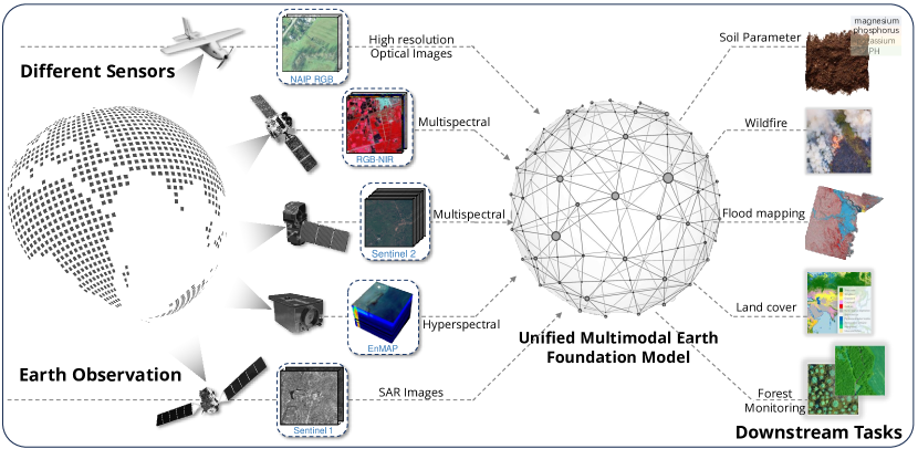
Figure 1: Overarching concept of multimodal foundation models. EO data consists of multiple modalities captured from different satellite sensors, such as NAIP, Gaofen, Sentinels, and EnMAP. The primary purpose of this work is to develop versatile foundation models capable of adaptively processing a wide array of EO data. This foundation model can be efficiently fine-tuned for diverse real-world downstream tasks, achieving specialized performance with minimal training samples and computational cost, thereby enhancing many EO applications.

One of the key challenges in developing EO foundation models is how to cope with multi-sensor data. Earlier methods were typically designed to specialize in a single data source or a specific range of spatial and spectral resolutions. For example, existing pretrained models like GFM ¹⁴, Scale-MAE ¹⁵, and Cross-scale-MAE ¹⁶ are pretrained for optical data. FG-MAE ¹⁷ and SatMAE ¹⁸ are developed for multi-spectral Sentinel-2 data, while SSL4EO-L ¹⁹ is designed for image data from Landsat. CROMA ²⁰ designs two unimodal encoders to encode multi-spectral and synthetic aperture radar (SAR) data. A cross-modal radar-optical transformer is utilized to learn unified deep representations. DeCUR ²¹ is a bimodal self-supervised model that decouples the unique and common representations between two different modalities. SpectralGPT ²² is a foundation model tailored for hyperspectral remote sensing data. It designs a 3D masking strategy, a spatial-spectral mixed encoder, and a decoder to preserve spectral characteristics for data reconstruction. Additionally, Satlas ²³ comprises a large-scale dataset from various sensors, with individual pretrained models provided for each sensor.

Current FMs for processing EO data often fall short of harnessing the full spectrum of information available, as they tend to focus narrowly on a single sensor modality or use distinct vision encoders for each type of sensor data. This strategy, while functional, does not tap into the vast potential offered by the optimum fusion of complementary information provided by multmodal data. Moreover, a critical limitation of these existing approaches is their lack of flexibility when adapting to diverse downstream tasks, which deviates from the original intent of designing FMs. In this regard, both the development of separate FMs and the extraction of multi-sensor features using separate visual encoders fail to account for this inter-sensor relationship, leading to the following limitations:

• The learned multimodal representation may not effectively capture such an inter-sensor relationship.

• The performance of foundation models will degrade when downstream tasks require the utilization of data from unseen sensors with varying numbers of spectral bands and spatial resolutions or different wavelength regimes.

• The development of individual, customized foundation models requires considerably more computing resources and human efforts.

• The increasing number of specialized foundation models makes it difficult to select the most appropriate one for a specific downstream task.

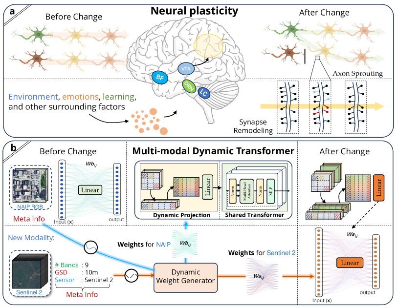
Figure 2: Motivation and main architecture of DOFA. Neuroplasticity ^{24, 25, 26} is an important brain mechanism for adjusting to new experiences or environmental shifts. Inspired by this concept, we design DOFA to emulate this mechanism for processing multimodal EO data. (a) Illustration of axon sprouting and synapse remodeling. These two types of neuroplasticity represent the brain’s capability to adapt its structure and function to learned information, experience, or injury. (b) Illustration of the core idea of DOFA. Similar to the principles of neuroplasticity observed in the human brain, DOFA is designed to adaptively alter its network weights in response to novel data modalities.

We aim to address these limitations and develop versatile FMs capable of adaptively processing this wide array of EO data, as illustrated in Fig. 1. Specifically, we propose to build an adaptive foundation model to overcome the inefficiencies and complexities of employing separate vision encoders for each data type. To this end, we draw inspiration from the concept of neuroplasticity in neuroscience ^{24, 25, 26, 27, 28}. Neuroplasticity embodies the dynamic ability of the brain to reorganize and adapt its neural connections in response to varying stimuli, experiences, and environmental changes. As shown in Fig. 2 (a), axon sprouting ²⁹ and synapse remodeling ³⁰ are two different types of neuroplasticity. It is an essential brain mechanism for adjusting to new experiences or environmental shifts ³¹. Drawing inspiration from this concept, we propose a Dynamic One-For-All model (DOFA), designed to emulate a dynamic mechanism for processing multimodal EO data. As shown in Fig. 2 (b), DOFA is designed to adaptively alter its network weights in response to novel data modalities ³².

DOFA employs an innovative approach utilizing wavelength as a unifying parameter across various EO modalities to achieve a more cohesive multimodal representation. At its core, the model integrates a hypernetwork ³³ that dynamically generates network weights based on the central wavelengths of each spectral band. This dynamic weight generator adjusts network weights to align with the specific modality of the input data, facilitating a customized network for each modality. Additionally, DOFA integrates a shared vision backbone, acting as a universal feature learning module for all heterogeneous data modalities. This framework enhances the model’s capacity to learn shared representations across diverse modalities. DOFA is trained using a masked image modeling strategy, and a distillation loss is included to further optimize its performance. This strategy facilitates quicker model convergence to reduce computational costs and enhances model performance by leveraging powerful representations from models pretrained on the ImageNet dataset ³⁴.

In the evaluation phase, we thoroughly test DOFA on diverse real-world tasks, showing that it surpasses current leading foundation models in most downstream (12 out of 13) datasets. This performance, achieved with a singular network using identical pretraining, underscores DOFA’s superior handling of multimodal EO data. DOFA mirrors the dynamic learning of the human brain for continuous model improvement from diverse data sources, making it highly adaptable for remote sensing’s broad data spectrum. The experimental results showcase DOFA’s versatility and effectiveness and confirm DOFA as a novel foundation model for analyzing complex remote sensing data. Although DOFA is proposed for analyzing EO data, its methodology can be widely applied to other domains where multimodal data is the mainstream such as medical image analysis, robotics, and climate modeling.

Results

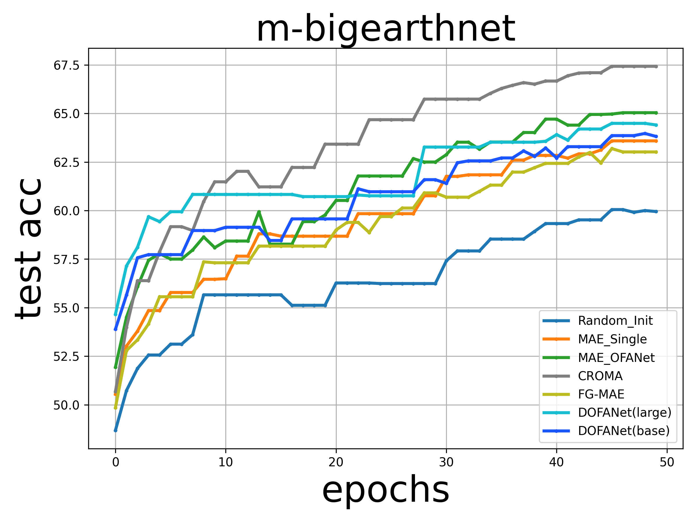
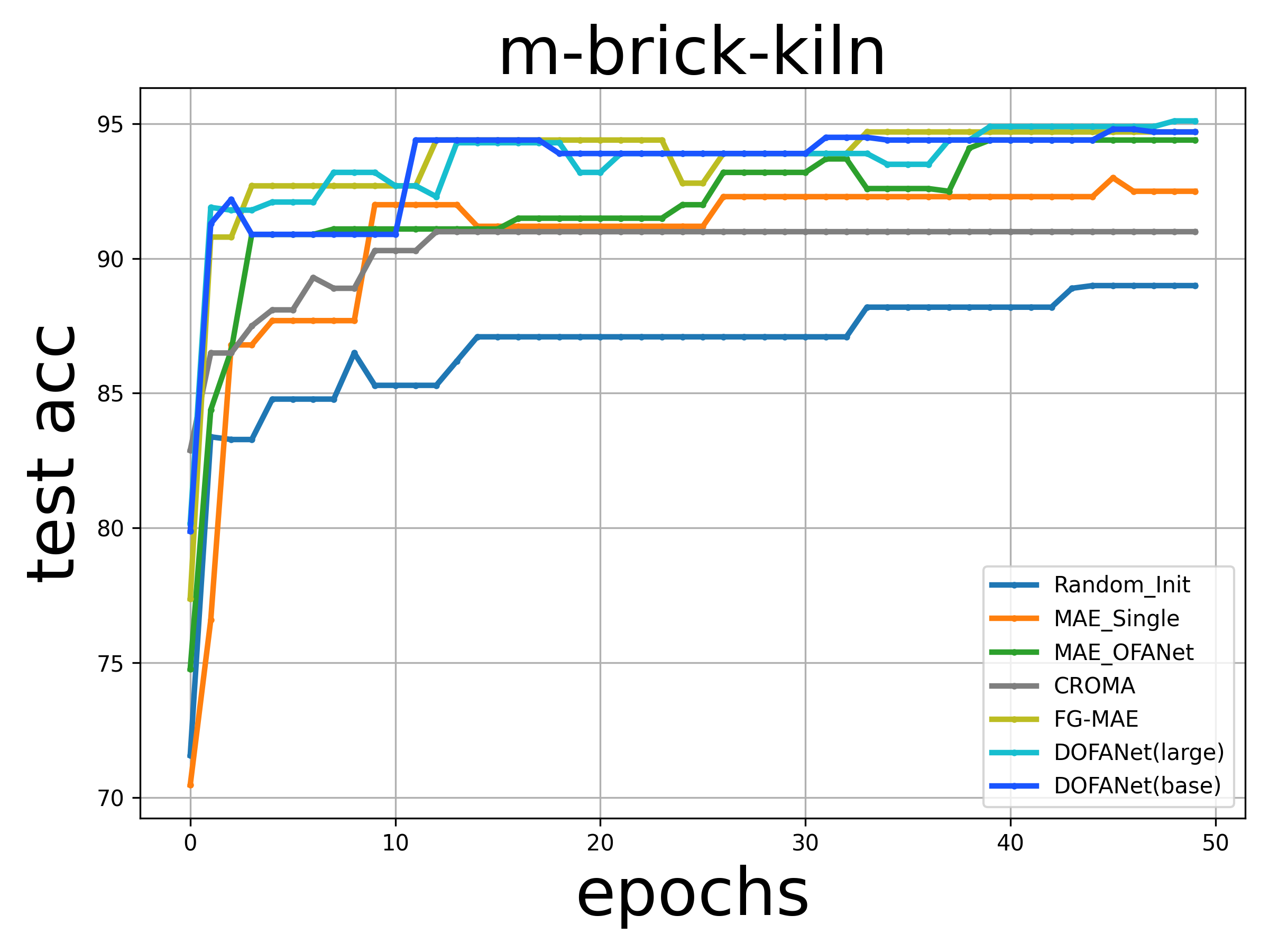
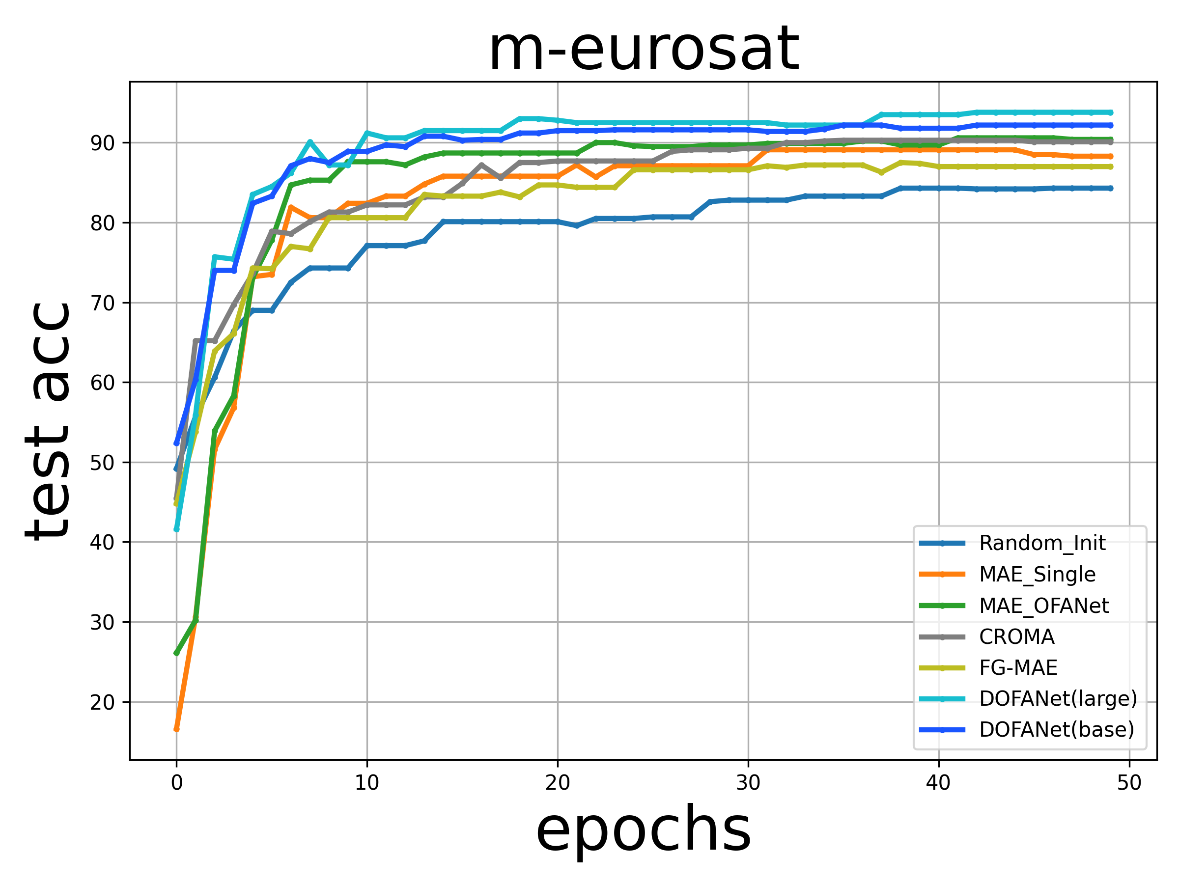
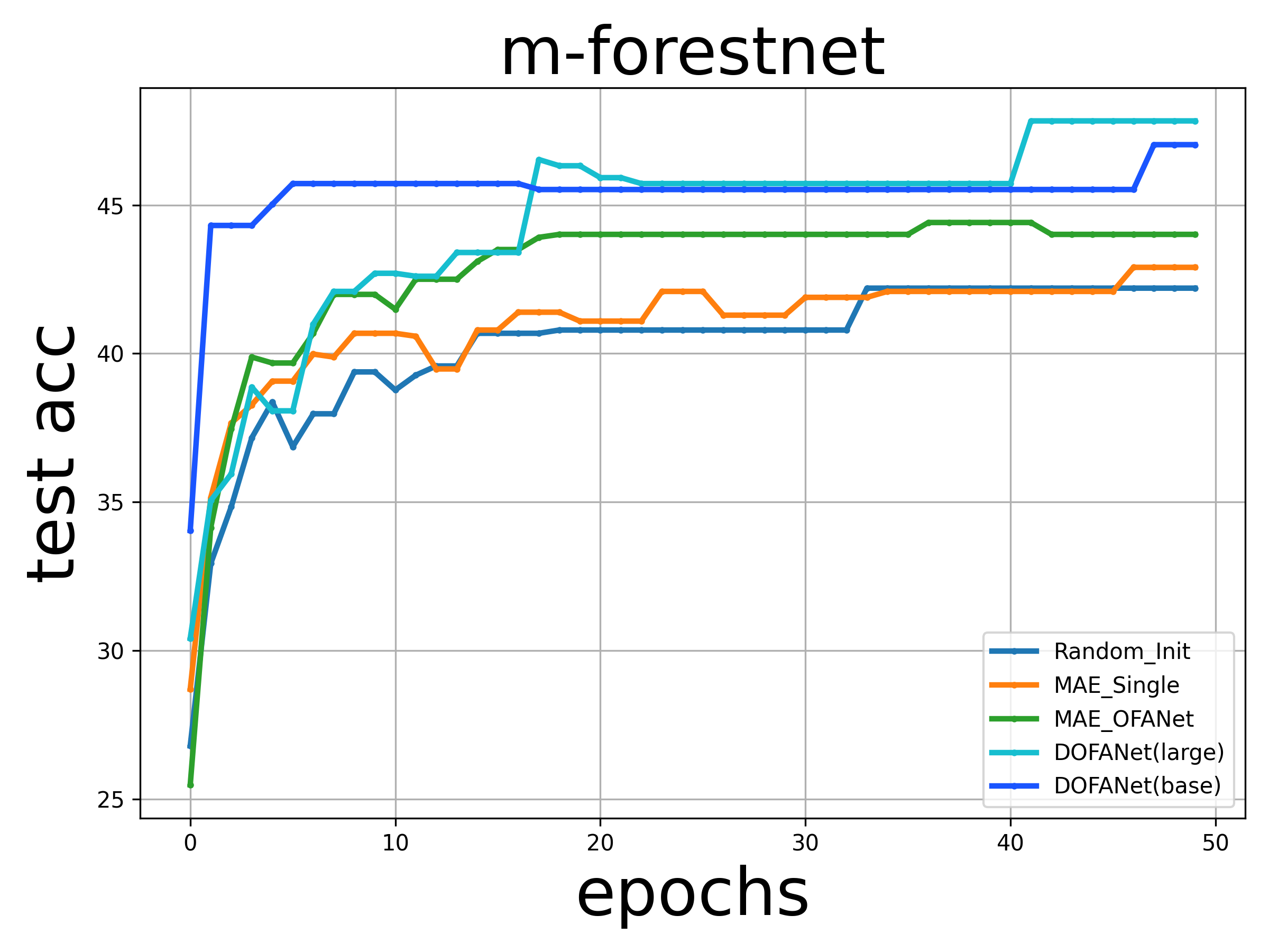
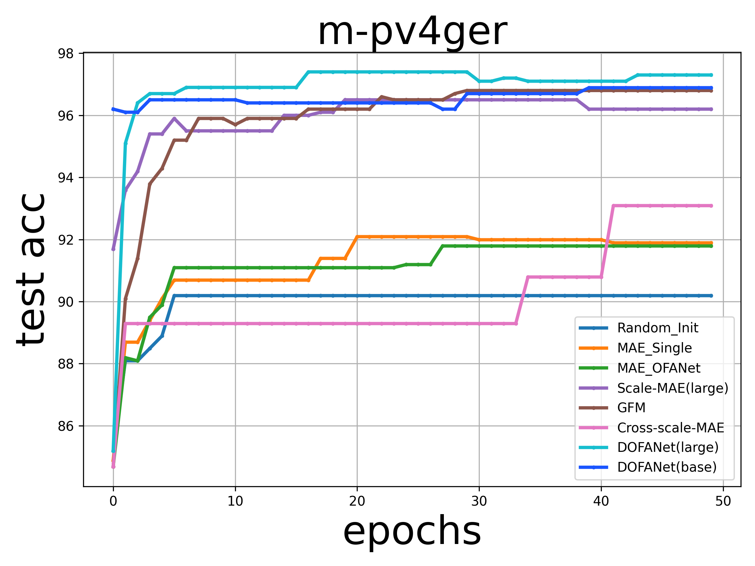
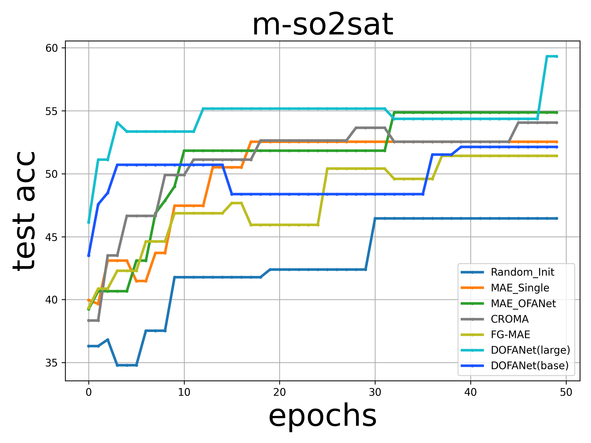
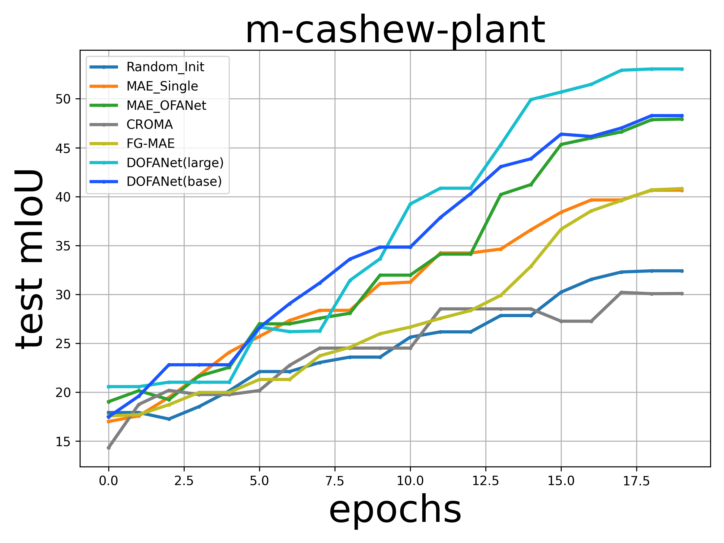
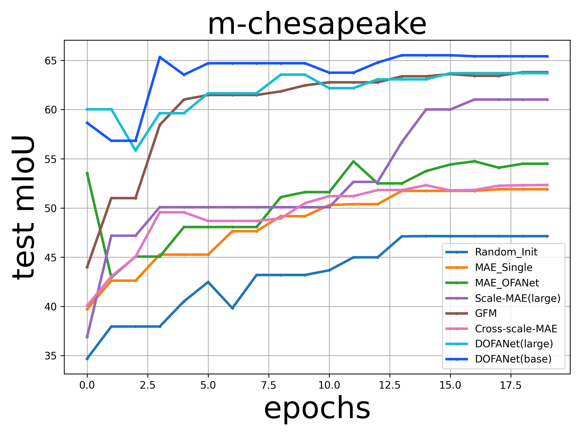
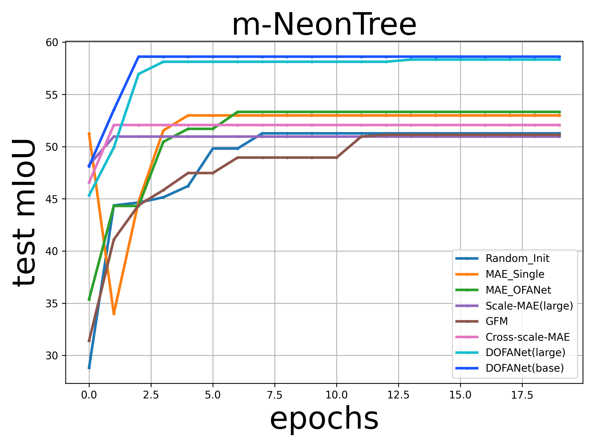
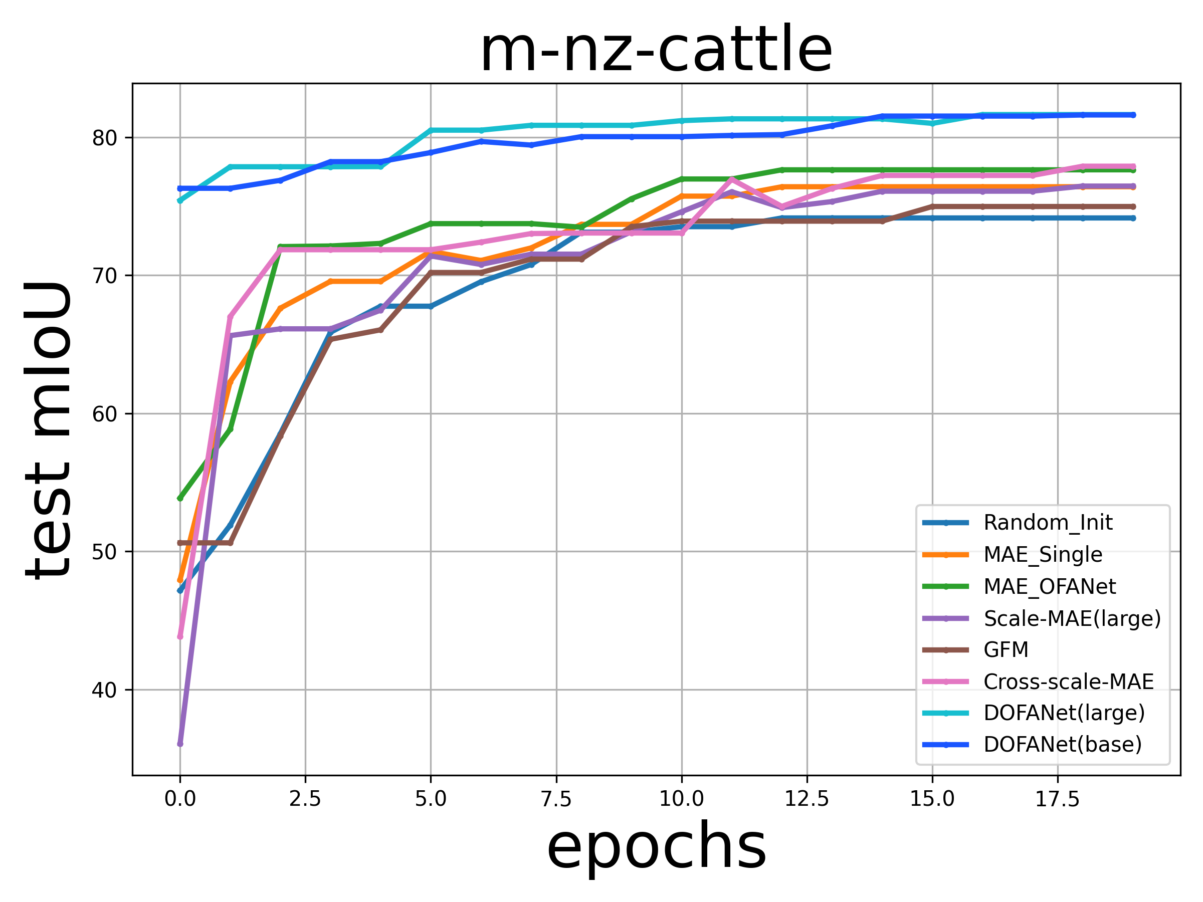
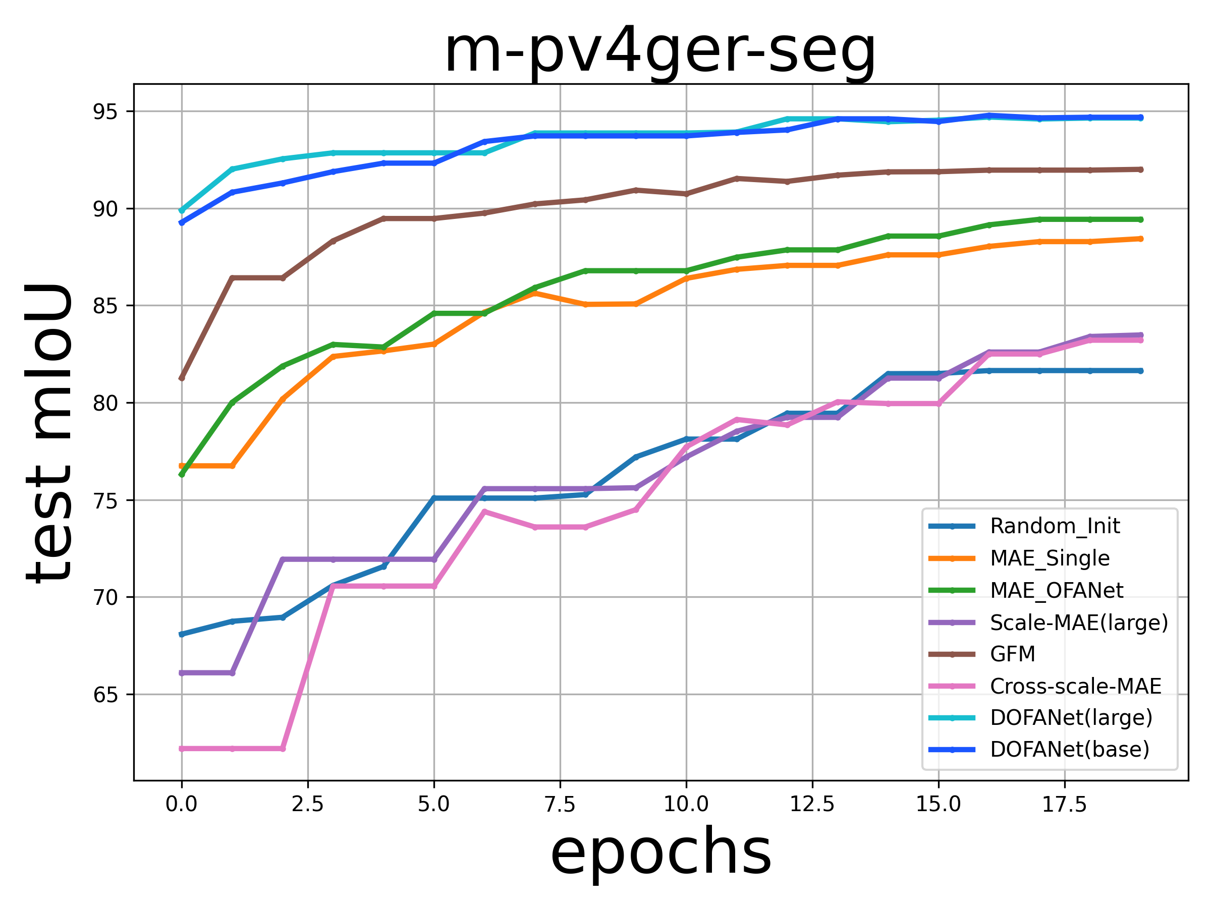
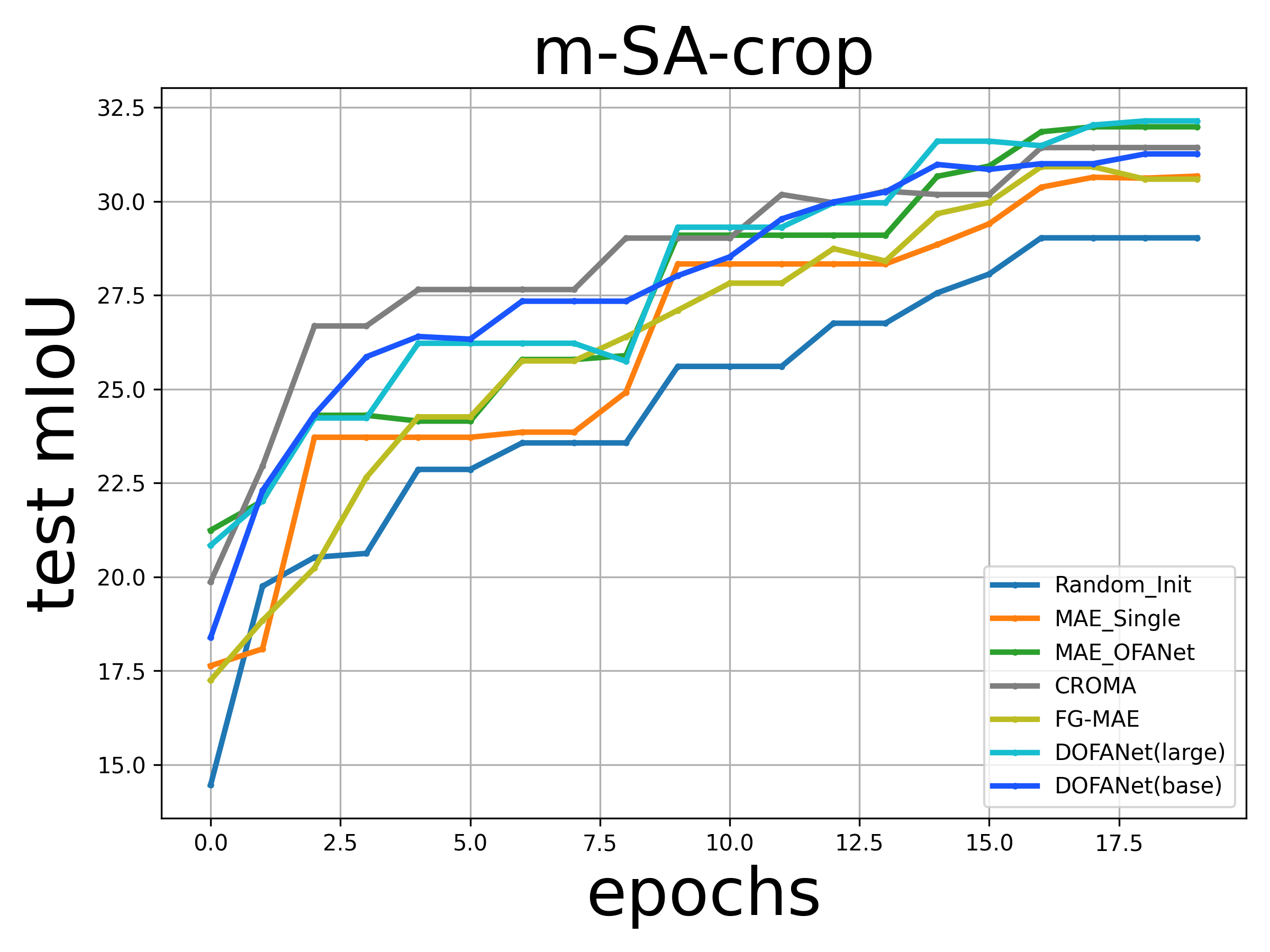
Figure 3: Visualization of accuracy curves for various foundation models. All results are for fine-tuning experiments on the GEO-Bench dataset. (rows 1 and 2) Top-1 accuracy for classification datasets. (rows 3 and 4) Mean intersection over union (mIoU) for segmentation datasets. It can be seen that DOFA converges faster and achieves better performance than other models on most datasets.

An effective unified multimodal foundation model would offer pretrained weights well characterizing the underlying training data, and lead to excellent performances on a wide range of downstream tasks and datasets (see details in Supplementary Materials C) compared to existing state-of-the-art (SOTA) foundation models after fine-tuning, and outperform individual FMs trained on a single modality. To comprehensively analyze the model performance, we organized our experiments as follows:

• We showcase the performance of using fully-supervised training with ImageNet pretrained weights on the GEO-Bench ³⁵ datasets. This comparison highlights the energy efficiency of foundation models when achieving comparable or superior performance to fully supervised models.

• To demonstrate the value of using pretrained weights, we provide linear probing results from the ViT model initialized with random weights.

• We present results from models trained exclusively on a single data modality to highlight the benefits of leveraging multiple data modalities.

• We compare DOFA with existing SOTA foundation models that provide pretrained model weights, including Scale-MAE ¹⁵, GFM ¹⁴, Cross-Scale MAE ¹⁶, CROMA ²⁰, FG-MAE ¹⁷, and OFA-Net ³⁶.

• We conduct full fine-tuning and linear probing experiments on the RESISC-45 dataset to compare with existing SOTA foundation models.

Note that for linear probing all models are trained for 50 epochs with only one linear layer trainable in the transfer learning setting. For the fine-tuning experiments, all parameters of the models are trained with sufficient epochs until convergence. Supplementary Materials A, B, and D provide more detailed information about the compared models and DOFA implementation.

Table 1: Linear probing results on six classification tasks. All models are trained for 50 epochs. The reported numbers are top-1 overall accuracy (OA). Missing values are due to the inability of the model to adapt to this domain.

Method	Backbone	m-bigearthnet	m-forestnet	m-brick-kiln	m-pv4ger	m-so2sat	m-eurosat
Fully Trained	ViT-S	66.0	53.8	98.1	97.6	57.5	97.3
Fully Trained	SwinV2-T	70.0	58.0	98.7	98.0	56.1	97.4
Fully Trained	ConvNext-B	69.1	56.8	98.9	98.0	58.1	97.7
rand. init.	ViT-B	52.9	41.5	84.5	91.3	38.3	85.7
MAE_Single 37	ViT-B	63.6	-	88.9	92.2	50.0	89.0
OFA-Net 36	ViT-B	65.0	-	94.7	93.2	49.4	91.9
SatMAE 18	ViT-B	62.1	-	93.9	-	46.9	86.4
Scale-MAE 15	ViT-L	-	-	-	96.9	-	-
GFM 14	Swin-B	-	-	-	96.8	-	-
Cross-Scale MAE 16	ViT-B	-	-	-	93.1	-	-
FG-MAE 17	ViT-B	63.0	-	94.7	-	51.4	87.0
CROMA 20	ViT-B	67.4	-	91.0	-	49.2	90.1
DOFA	ViT-B	63.8	45.3	94.7	96.9	52.1	92.2
DOFA	ViT-L	64.4	47.4	95.1	97.3	59.3	93.8

Table 2: Fine-tuning results on six segmentation tasks. All models are trained with a frozen backbone for 20 epochs. Reported numbers are mean intersection over union (mIoU). Missing values are due to the inability of the model to adapt to this domain.

Method	Backbone	m-pv4ger-seg	m-nz-cattle	m-NeonTree	m-cashew-plant	m-SA-crop	m-chesapeake
DeepLabv3	ResNet101	93.4	67.6	53.9	48.6	30.4	62.1
U-Net	ResNet101	94.1	80.5	56.6	46.6	29.9	70.8
rand. init.	ViT-B	81.7	74.1	51.7	32.4	29.0	47.1
MAE_Single 37	ViT-B	88.4	76.4	53.0	40.7	30.7	51.9
OFA-Net 36	ViT-B	89.4	77.6	53.3	47.9	31.9	54.5
Scale-MAE 15	ViT-L	83.5	76.5	51.0	-	-	61.0
GFM 14	Swin-B	92.0	75.0	51.1	-	-	63.8
Cross-Scale MAE 16	ViT-B	83.2	77.9	52.1	-	-	52.3
CROMA 20	ViT-B	-	-	-	30.1	31.4	-
FG-MAE 17	ViT-B	-	-	-	40.8	30.6	-
DOFA	ViT-B	94.7	81.6	58.6	48.3	31.3	65.4
DOFA	ViT-L	95.0	81.7	59.1	53.8	32.1	66.3

DOFA masters in arbitrary classification tasks

The results on six classification downstream tasks are presented in Table 1. “Fully Trained” denotes the models using ImageNet pretrained weights for transfer learning and fully training the model on each dataset individually. We report the results of three different backbones on the GEO-Bench dataset, including ViT-S ³⁸, SwinV2-T ³⁹, and ConvNext-B ⁴⁰.

Although these models can perform better than self-supervised learning models in the linear probing setting, they require significantly higher cost, time, and energy training expenses. Moreover, adapting each distinct network architecture to various datasets demands substantial efforts in hyper-parameter tuning. In contrast, pretrained weights can save training costs and time. Merely 50 epochs of linear probing with pretrained weights can yield performance comparable to fully trained models, highlighting the advantage of EO foundation models.

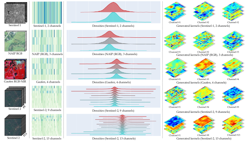
Figure 4: Visualization of the dynamic weight generator. From left to right: examples of input images, learned embeddings for different central wavelengths, the histogram distributions of the generated weights, and some examples of the generated kernel weights.

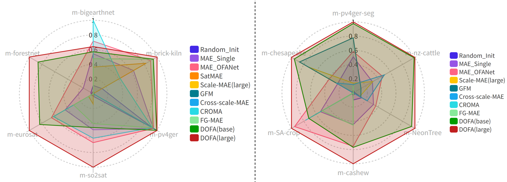
Figure 5: Performance of different foundation models on GEO-Bench. DOFA, a single unified foundation model, can outperform most of the specifically trained SOTA foundation models on both (a) classification datasets and (b) segmentation datasets. These results demonstrate the effectiveness and versatility of DOFA. For clarity in the radar chart, min-max normalization has been applied.

We compare seven different SOTA self-supervised models. We can see that the data from other datasets has diverse spectral bands. Aside from the proposed DOFA, no existing model is universally adaptable for all downstream tasks in the transfer learning setting. For example, the “m-forest” dataset contains images from Landsat 8, which differs from all the data modalities used to train the compared models. However, in this case, the proposed DOFA can still be used for linear probing, even though it has never seen Landsat imagery during pre-training. This demonstrates that individually developed foundation models for a single modality have limitations when applied to real-world EO applications. DOFA is flexible enough to apply to all EO data modalities.

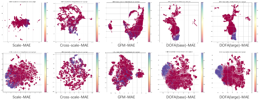
(a) m-pv4ger dataset.

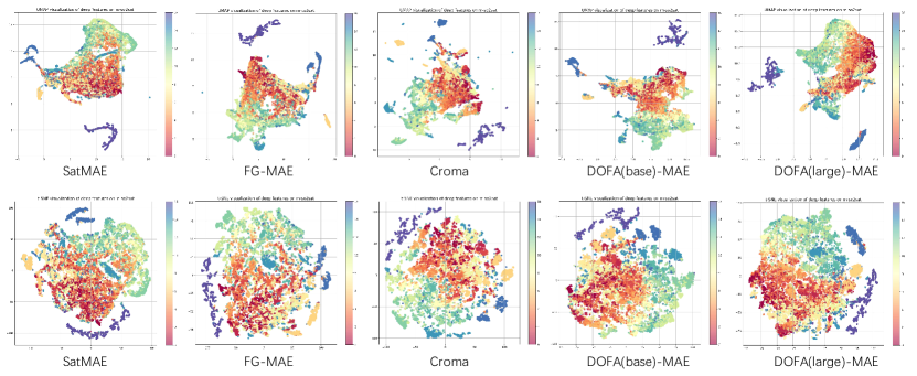
(b) m-so2sat dataset.

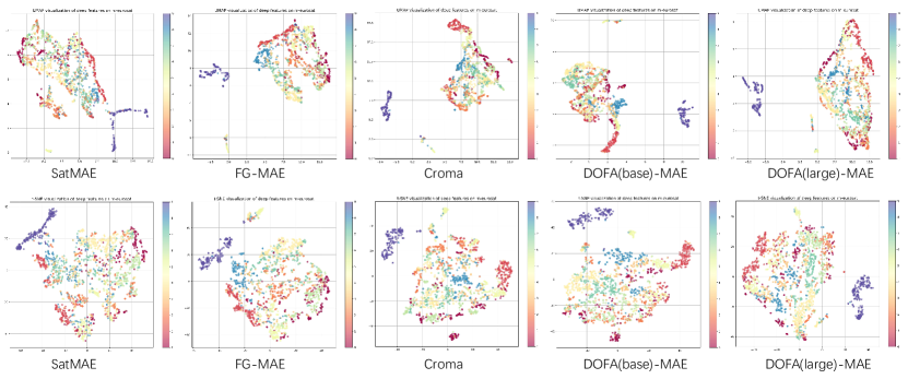
(c) m-eurosat dataset.

Figure 6: Visualization of learned embeddings. (row1) UMAP and (row 2) t-SNE plots of the feature representations from various foundation models across multiple datasets. Enhanced separability signifies more effective representations.

Regarding performance, DOFA obtains the best results on all datasets except the “m-bigearthnet” dataset. DOFA uses a single pretrained model without switching to different pretrained weights or network architectures. This indicates that DOFA effectively transfers to different downstream tasks, even for new sensors (Landsat 8). This comparison with fully supervised training results highlights that foundation models, with minimal and energy-efficient fine-tuning, can achieve comparable or superior performance to that of extensively supervised trained models. On the “m-bigearthnet” dataset, although the performance is not the best, it is still competitive compared with other SOTA models. Notably, on the “m-so2sat” dataset, DOFA with ViT-Large backbone achieves a top-1 overall accuracy of 59.3%, even higher than the fully trained models. The comparison results reveal that DOFA, designed to serve a general purpose, is a promising EO foundation model that can be effective in various downstream tasks.

We visualize the accuracy curves of different SOTA models in Fig. 3 for the classification and segmentation datasets. These figures show that the proposed DOFA converges faster than other models and achieves better performance on the majority of datasets. We visualize the learned embeddings of various wavelengths and the generated kernels for different sensors in Fig. 4 for a better understanding of DOFA. We randomly select and plot six $16\times 16$ kernel weights for input images with more than four channels. The figures indicate that DOFA can generate weights for different sensors dynamically and effectively.

DOFA outperforms single-source models for segmentation tasks

The results on six segmentation tasks are displayed in Table 2. For the segmentation tasks, we compare two types of models. One is a fully-trained model using the ResNet101 backbone and pretrained weights on ImageNet. The other type is each model pretrained using self-supervised methods. For these models, we freeze the weights of their backbone and only fine-tune the segmentation head. To ensure a fair comparison, UPerNet ⁴¹ is used for all these models as the segmentation head. The results show that DOFA performs even better than the fully trained DeepLabv3 and U-Net models. Note that DOFA models only train the segmentation head for 20 epochs, which is fast and energy-efficient. Compared with other foundation models, the results of DOFA with ViT-Base and ViT-Large backbones show clear superiority, especially on the “m-NeonTree” and the “m-nz-cattle” datasets. The performance across six segmentation tasks further validates DOFA’s versatility as an EO foundation model, which can support both classification and segmentation downstream tasks.

Similarly, we visualize the accuracy curves of different models in Fig. 3 for these six segmentation datasets. Observations indicate that DOFA achieves superior accuracy and faster convergence than other SOTA models. To concisely illustrate the comparative performance of these models across various datasets, we employ a radar chart. Fig. 5 (a) reveals that DOFA models achieve impressive performance across all six datasets, highlighting the model’s versatility and efficiency. Similarly, Fig. 5 (b) shows that DOFA demonstrates robust applicability across diverse downstream tasks.

Table 3: Classification results on the RESISC-45 dataset.

Methods	Backbone	Frozen	Finetune
Scale-MAE	Vit-Large	89.6	95.7
SatMAE	Vit-Large	88.3	94.8
ConvMAE	ConvVit-Large	81.2	95.0
Vanilla MAE	Vit-Large	88.9	93.3
DOFA	Vit-Base	91.3	93.8
DOFA	Vit-Large	91.9	96.1

In addition to the datasets in GEO-Bench, we compare DOFA with existing foundation models on the RESISC-45 dataset ⁴² and present the results in Table 3. The linear probing (frozen) and fully fine-tuned settings are used for performance comparison. The results are shown in Table 3. For fully fine-tuning the RESISC-45 dataset, we train both models (ViT-Base and ViT-Large) for 100 epochs with a base learning rate of 4$e$-3 and a weight decay of 5$e$-3. Note that the learning rate on the backbone is multiplied by 0.1. We set the learning rate to 0.1 for the liner probing setting and the weight decay to 0.05. When the backbone is frozen, DOFA (ViT-Large) can achieve a top-1 overall accuracy of 91.9%, significantly better than other models. For the fully fine-tuning results, DOFA also outperforms existing models, demonstrating its effectiveness.

DOFA optimizes separability in latent space

We visualize the pretrained representations of different models using two types of dimensionality reduction techniques used to represent high-dimensional data, UMAP ⁴³ and t-SNE ⁴⁴. Specifically, the extracted features of the pretrained models on downstream dataset m-pv4ger, m-so2sat, and m-eurosat are shown in Fig. 6(a), 6(b), and 6(c), respectively. Different colors represent different semantic categories. On these three datasets, the learned features of both versions of DOFA are clustered better than those of other compared models. These figures further validate the effectiveness of the proposed DOFA as a unified EO foundation model.

Discussion and conclusions

In this work, we present a multimodal foundation model, inspired by neural plasticity. This innovative “dynamic one-for-all” framework is adept at handling an extensive variety of data types, modalities, and spatial resolutions. Emulating the human brain’s adaptability, it processes diverse data modalities with unprecedented versatility and efficiency. The proposed DOFA successfully demonstrates the enhanced utility and effectiveness of foundation models for diverse downstream tasks. This achievement underscores the potential of our dynamic model to revolutionize the way we interpret and analyze Earth’s spatial data.

While we have achieved significant milestones, challenges persist in refining the model’s performance across different data modalities, particularly through the advancement of multimodal pre-training techniques. The future presents expansive opportunities for DOFA, aiming to extend its applications across a wider spectrum of data types and tasks, and to incorporate more varied data modalities such as LiDAR point clouds and textual data. Future iterations of DOFA will prioritize integrating diverse data modalities including time-series data to enhance the understanding of Earth’s dynamics. This unified approach aims at revolutionizing applications in Earth system modeling, as well as weather and climate analysis, by providing a comprehensive view of environmental processes.

Methods

Here, we provide detailed information about the proposed DOFA model and a more detailed presentation of the training method.

Mathematical formalism

Given an input image $\mathbf{X}\in\mathbb{R}^{C\times H\times W}$, where $H$, $W$, and $C$ represent the height, width, and number of channels, respectively, the image is first divided into a patch sequence. Each patch has a fixed spatial size $P\times P$ with $C$ channels, and thus the image is converted into $N=\frac{HW}{P^{2}}$ patches. Each patch is flattened into a vector and linearly transformed into a $D$-dimensional embedding. This transformation is represented by a trainable embedding matrix $\mathbf{E}\in\mathbb{R}^{P^{2}C\times D}$.

Formally, the patch embedding can be described as:

$$\mathbf{X}=[\mathbf{X}_{p_{1}};\mathbf{X}_{p_{2}};\ldots;\mathbf{X}_{p_{N}}],\quad\mathbf{X}_{p_{i}}\in\mathbb{R}^{P^{2}C},$$ (1)

where $\mathbf{X}_{p_{i}}$ is the flattened vector of the $i$-th patch. Next, the flattened vectors are linearly projected into $D-$dimensional embeddings with a learnable embedding matrix:

$$\mathbf{Z_{0}}=[\mathbf{X}_{p_{1}}\mathbf{E};\mathbf{X}_{p_{2}}\mathbf{E};\ldots;\mathbf{X}_{p_{N}}\mathbf{E}],\quad\mathbf{Z_{0}}\in\mathbb{R}^{N\times D},$$ (2)

where $\mathbf{Z}_{0}$ represents the sequence of patch embeddings. Note that this process can be implemented utilizing a single convolution layer with a $P\times P$ kernel, $C$ input channels, and $D$ output channels. Class token $\mathbf{X}_{\text{cls}}$, an additional learnable embedding, is prepended to the sequence. Finally, position embeddings are added to retain positional information.

$$\mathbf{Z^{\prime}}=[\mathbf{X}_{\text{cls}};\mathbf{Z_{0}}]+\mathbf{E_{\text{pos}}},\quad\mathbf{Z^{\prime}}\in\mathbb{R}^{(N+1)\times D},$$ (3)

Here, $\mathbf{E_{pos}}$ denotes the position embeddings, and the resulting $\mathbf{Z^{\prime}}$ serves as the input to the subsequent layers of the ViT architecture.

Architecture overview

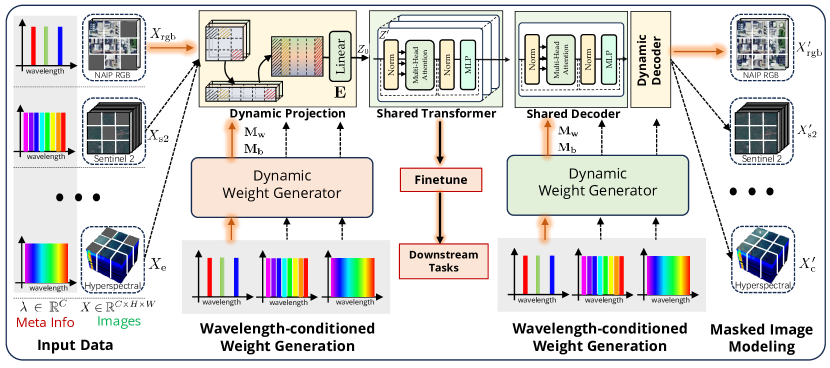
Figure 7: Overall architecture design. DOFA builds on the principles of masked image modeling, introducing a significant advancement by processing input images with any number of channels. This is enabled through the designed hypernetwork-based dynamic weight generator, which adapts to the spectral wavelength of each channel. By embedding images with varying channel numbers into a unified feature space, the model leverages shared Transformer blocks to learn modality-shared representations. This architecture enables the model to learn versatile multimodal representations and handle diverse data modalities within a single framework.

The patch embedding layer transforms the input image into a sequence of embeddings that the self-attention mechanism of the Transformer can process. A straightforward way to handle the input data from different modalities is to utilize multiple patch embedding layers to convert data with different spectral wavelengths into embeddings with the same dimension ³⁶. Suppose that the input image $\mathbf{X}$ of dimensions $\mathbb{R}^{C\times H\times W}$ can originate from various data modalities. Initially, images from different sources are standardized to height $H$ and width $W$. Specifically, we consider five distinct modalities: Sentinel 1 data ($\mathbf{X}_{\text{s1}}$) with 2 SAR channels ($\mathbb{R}^{2\times H\times W}$), Sentinel 2 data ($\mathbf{X}_{\text{s2}}$) with nine multispectral channels ($\mathbb{R}^{9\times H\times W}$), Gaofen data ($\mathbf{X}_{\text{g}}$) with four multispectral channels ($\mathbb{R}^{4\times H\times W}$), NAIP imagery ($\mathbf{X}_{\text{rgb}}$) with 3 RGB channels ($\mathbb{R}^{3\times H\times W}$), and EnMAP data ($\mathbf{X}_{\text{e}}$) with 202 available hyperspectral channels ($\mathbb{R}^{202\times H\times W}$). Note that, for the sake of simplicity, we omit the batch size for the denotation of tensors. OFA-Net ³⁶ proposes a simple and straightforward way to use individual patch embedding layers for each data modality. However, although practical, this method is not flexible enough when the number of bands of downstream tasks changes.

In this context, inspired by the brain’s neuroplasticity, we propose a dynamic architecture to flexibly adapt the model to different modalities and handle variations in the number of spectral bands, as illustrated in Fig. 7. The whole architecture follows the design of masked image modeling (MIM) ³⁷. The main difference from traditional masked autoencoders (MAE) lies in DOFA’s capacity to process input images with various channels. This flexibility is achieved through a hypernetwork-based dynamic weight generator, a critical component of the model’s design. The dynamic weight generator takes inputs from the spectral wavelength associated with each image channel and predicts the patch embedding matrix $\mathbf{E}$ for different data modalities dynamically to learn specific representations for each modality. The latent representations are then passed through a series of shared Transformer blocks for learning generalizable multimodal representations. These blocks apply self-attention mechanisms to capture the complex interactions between different image parts.

Parallel to the dynamic weight generation for the encoder part of the network, the dynamic decoder is responsible for reconstructing the output image from the encoded latent space. Similarly, the dynamic decoder utilizes another set of dynamically generated weights to ensure that the reconstructed image matches the number of spectral bands of the target modality. We employ a MIM strategy to train this self-supervised architecture. The input images are masked randomly, and the model learns to reconstruct these missing parts. As the parameters in DOFA are learned across different modalities, this process helps learn robust multimodal representations beneficial for various EO tasks. After the pertaining process, the model can be finetuned for specific downstream tasks with fewer learnable parameters and training costs to tailor the model to specific EO applications without extensive retraining. The model can be transferred to various EO applications by integrating dynamic weight generation and decoding, from high-resolution optical imaging to multispectral and hyperspectral sensing.

Wavelength-conditioned dynamic patch embedding

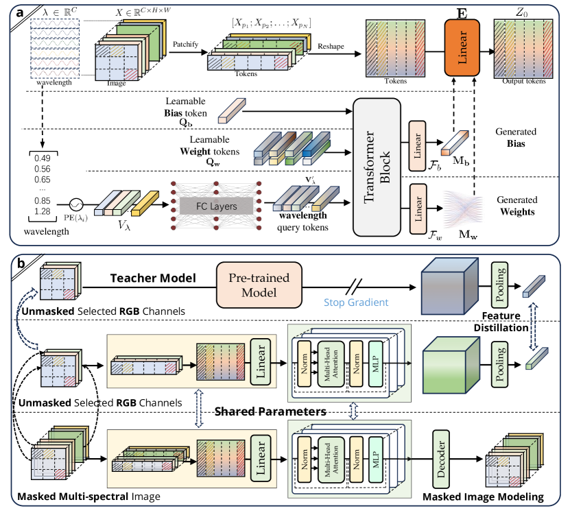
Figure 8: Dynamic weight generator and continual training framework. (a) The central wavelengths of each band are first transformed into high-dimensional features for an input image. Subsequently, a Transformer encoder layer and two fully-connected layers derive the dynamic weights and biases tailored to each wavelength. Finally, these dynamically generated weights and biases are employed in the convolution operation to create a patch embedding. (b) Continual pretraining process. There are two loss terms: one distillation and one reconstruction loss.

To manage the diversity of spectral bands across different modalities, we project the data into a latent space with uniform feature dimensionality using the dynamic patch embedding layer $\mathcal{F}_{\text{dpe}}$. As described in Mathematical formalism, we denote the input image as $\mathbf{X}\in\mathbb{R}^{C\times H\times W}$. Fig. 8 (a) illustrates the detailed steps used to compute the dynamic weights given the wavelength information of each channel. Each channel of the input image has a corresponding central wavelength. The wavelengths of an input image with $C$ channels can be represented by $\mathbf{\lambda}\in\mathbb{R}^{C}$. To convert the wavelengths to a higher-dimensional feature space, we encode the wavelengths $\lambda$ using a 1D sine-cosine positional encoding:

$$\mathbf{V_{\lambda}}=\text{PE}(\mathbf{\lambda})\in\mathbb{R}^{C\times D_{\lambda}},$$ (4)

The positional encoding $\text{PE}(\lambda_{i})$ for wavelength $\lambda_{i}$ in channel $i$ is given by:

$$\text{PE}(\lambda_{i},2k) =\sin\left(\frac{\lambda_{i}}{10000^{2k/D_{\lambda}}}\right),$$ (5)

$$\text{PE}(\lambda_{i},2k+1) =\cos\left(\frac{\lambda_{i}}{10000^{2k/D_{\lambda}}}\right),$$

where $k=0,\ldots,\frac{D_{\lambda}}{2}-1$. This process embeds each wavelength into a $D_{\lambda}$-dimensional feature vector. The positionally encoded wavelengths $\mathbf{V}_{\lambda}$ are further transformed through two fully-connected layers with residual connections:

$$\mathbf{\mathbf{V^{\prime}}_{\lambda}}=\text{ReLU}(\mathcal{F}_{2}(\text{ReLU}(\mathcal{F}_{1}(\mathbf{V}_{\lambda}))))+\mathbf{V}_{\lambda},$$ (6)

where $\mathcal{F}_{1}$ and $\mathcal{F}_{2}$ represent the fully-connected layers, and ReLU denotes the Rectified Linear Unit activation function ⁴⁵.

Next, we employ a Transformer encoder ⁴⁶ layer with four attention heads to generate the dynamic weights and bias for each wavelength. Specifically, the embedding $\mathbf{V^{\prime}_{\lambda}}$, $N_{w}$ learnable query tokens $\mathbf{Q_{w}}$, and one learnable bias query token $\mathbf{Q_{b}}$ are concatenated together to form the input to the Transformer encoder:

$$\mathbf{V^{\prime\prime}}=\text{TransformerEncoder}(\text{Concat}(\mathbf{V^{\prime}}_{\lambda},\mathbf{Q_{w}},\mathbf{Q_{b}})).$$ (7)

We subsequently extract the embeddings $\mathbf{V^{\prime\prime}}_{w}$ that correspond to the weight query tokens $Q_{w}$ from $\mathbf{V^{\prime\prime}}$, as well as the embeddings $\mathbf{V^{\prime\prime}}_{b}$ associated with the bias query tokens $\mathbf{Q_{b}}$ from $\mathbf{V^{\prime\prime}}$. Then, two fully-connected layers are utilized to generate the dynamic weights and biases:

$$\mathbf{M_{w}} =\mathcal{F}_{w}(\mathbf{V^{\prime\prime}}_{w}+\mathbf{V^{\prime}}_{\lambda})\in\mathbb{R}^{C\times P^{2}D},$$ (8)

$$\mathbf{M_{b}} =\mathcal{F}_{b}(\mathbf{V^{\prime\prime}}_{b})\in\mathbb{R}^{C\times D},$$

where $\mathcal{F}_{w}$ and $\mathcal{F}_{b}$ denote the fully-connected layers for weight and bias generation, respectively. As introduced in Section Mathematical formalism, the patch embedding layer can be implemented efficiently using a convolution layer. Thus, we reshape the generated weights into the convolution kernel as:

$$\mathbf{K_{\text{conv}}}=\text{Reshape}(\mathbf{M_{w}},[D,C,P,P]),$$ (9)

The convolution operation for patch embedding is then performed using the dynamically generated weights $\mathbf{K_{\text{conv}}}$ and biases $\mathbf{M_{b}}$:

$$\text{PatchEmbedding}:=\text{Conv}(\mathbf{X},\mathbf{K_{\text{conv}}},\mathbf{M_{b}}),$$ (10)

where $\mathbf{X}$ is the input image, and Conv denotes the convolution operation.

Utilizing this approach, the patch embedding layer achieves independence from the number of spectral bands of the input images. The weights for these layers are dynamically generated based on the central wavelength of each channel in a compositional manner. This mechanism enables the model to learn modality-specific representations dynamically, thereby enhancing its adaptability and performance across various data domains.

For the wavelength-conditioned dynamic decoder, we use different parameters to generate dynamic weights and biases. The computation process is similar to the dynamic patch embedding layer described before. In the vanilla masked autoencoder, the final layer of the decoder is usually implemented as a fully-connected layer to convert features from latent space into pixel space. For the dynamic decoder layer, we follow the same process with the dynamic patch embedding to generate the dynamic weights. The only difference is that a fully-connected layer is used in the decoder rather than the convolution layer in the patch embedding layer.

Continual pretraining

The self-supervised loss formulation is pivotal for training our multimodal EO foundation model. The model leverages the MIM paradigm to circumvent the necessity for spatially aligned multimodal datasets, which are challenging to construct. To reduce the computational cost of self-supervised training on extensive datasets, we design a continual pretraining strategy inspired by Mendieta et al. ¹⁴ incorporating a distillation loss and a weight initialization strategy. This method effectively utilizes knowledge from expansive, supervised, pretrained models, reducing the computational burden and associated CO₂ emissions.

Given the disparities in spectral resolution between these datasets, using ImageNet pretrained weights for continual pretraining is challenging. Instead, we design a proxy-based distillation method that extracts optical data as a proxy to ensure representation similarity between the teacher and student networks. As illustrated in Fig. 8 (b), for multi-channel input data with more than three channels, we extract the RGB channels to form a 3-channel input $X_{p}\in\mathbb{R}^{3\times H\times W}$. We randomly select one channel for Sentinel-1 data with only two bands and duplicate it to a synthetic three-channel image. This input $X_{p}$ is then fed into an ImageNet-pretrained teacher model to get teacher features $F_{t}$. Concurrently, the dynamic encoder in DOFA is also used to encode $X_{p}$ into student features $F_{s}$. Throughout this procedure, the teacher model’s weights remain frozen to preserve structured representations and reduce the computational load during optimization.

We also follow a continual pretraining strategy for initializing the dynamic weight generator. First, we pretrain the generator to mimic the teacher model’s patch embedding layer weights. We then use the pretrained weights to initialize the dynamic embedding layer.

The training loss comprises two distinct components. One is the MIM reconstruction loss, which forces the model to predict $X^{\prime}\in\mathbb{R}^{C\times H\times W}$ for reconstructing various data modalities from the full-channel inputs $X$. The other one is the feature distillation loss, which employs the cosine similarity between the teacher and student feature representations to guide the learning process of the student model. Suppose that the encoded feature of the full channel input is $F$; then the composite loss function can be formulated as follows:

$$\mathcal{L}=\frac{1}{N}\sum_{i=1}^{N}\|X_{i}-X^{\prime}_{i}\|^{2}-\frac{\mathcal{F}_{P}(F_{si})\cdot F_{ti}}{\|\mathcal{F}_{p}(F_{si})\|_{2}\cdot\|F_{ti}\|_{2}},$$ (11)

where $\mathcal{F}_{P}$ is a linear projection layer. By employing this bifurcated loss function, our model’s training is supervised from two distinct perspectives. First, it leverages the complete spectral information present in the input to learn cross-modal features via image reconstruction. Second, it distills knowledge from extensively pretrained models into diverse data modalities using a single, shared dynamic model. This approach enables efficient and robust feature learning and is adept at handling the complexities of various modalities.

Data availability

The curated datasets and pre-trained model weights will be available at https://github.com/ShadowXZT/DOFA-pytorch and https://huggingface.co/XShadow/DOFA.

Code availability

Code is available at https://github.com/zhu-xlab/DOFA.

Supplementary materials

A. Related methods

Recently, foundation models ¹³ have showcased remarkable success in transferring to a broad range of downstream tasks within a unified paradigm. These transfer learning techniques include fine-tuning, zero-shot ⁴⁷, or few-shot ^{48, 49} learning, as well as instruction tuning ⁵⁰. Notable examples of foundation models encompass large language models like LLaMA ⁵¹, GPT-3 ⁵², and ChatGPT ⁵³, alongside prominent visual models such as CLIP ⁵⁴, BLIP ⁵⁵, Stable Diffusion ⁵⁶, and SAM ⁵⁷. One of the critical factors that contribute to the success of foundation models is self-supervised learning, with typical methods including BYOL ⁵⁸, DINO ⁵⁹, and MAEs ³⁷. These methods harness techniques like contrastive learning ⁶⁰ and next token prediction to enable the exploration of large-scale data without human annotation.

Real-world data are characterized by diverse modalities, including but not limited to images, videos, text, audio, depth information, and point clouds. The capacity of foundation models to effectively handle this variety in downstream tasks hinges on their ability to process multimodal data. In this context, visual-language foundation models have emerged as a preceding and significant area of research. These models are adept at developing a universal representation that seamlessly merges visual and language modalities. Their work encompasses a broad spectrum of visual-language understanding ⁵⁴ tasks, addressing different levels of granularity and facilitating various cross-modal reasoning applications like image-text retrieval ⁶¹ and image referring ⁶². Additionally, they extensively explore a wide range of text-based visual generation ⁵⁶ tasks.

A critical research question in developing multimodal foundation models is how to achieve a unified representation for various input modalities and output formats. Approaches capable of achieving such a representation are often referred to as a unified framework ^{63, 64}. A notable example is the Meta-Transformer ⁶⁵, which firstly employs a data-to-sequence tokenizer to convert data from 12 different modalities into a shared embedding space and later trains a shared encoder to generate the unified multimodal representation.

In EO, the necessity of a unified multimodal foundation model becomes increasingly significant. In contrast to natural scene images, EO data typically manifests diverse characteristics. It can be captured by various sensors such as Landsat, Sentinel, MODIS, EnMAP, and NAIP, featuring varying numbers of spectral bands, spatial resolutions, and temporal repeat periods. Despite these differences, the data from these sources often exhibit distinct yet related characteristics. For instance, optical, multispectral, and hyperspectral images may share similar attributes in bands with similar wavelengths. EO data with similar ground sampling distance (GSD) may exhibit higher similarity. This underscores the imperative for a more sophisticated approach to multimodal representation learning for EO data.

Early efforts in developing EO foundation models were devoted to generating effective embeddings for data from a single modality. Examples include SeCo ⁶⁶ and CaCo ⁶⁷, which leverage temporal information from acquired images to learn temporal-sensitive and temporal-invariant feature representations. GFM ¹⁴ devises a continual pretraining paradigm that leverages ImageNet pretrained features to accelerate model convergence on EO data. Cha et al. ⁶⁸ explore the impact of scaling up the number of parameters in foundation models, specifically on Google Earth images. Another line of research addresses the adaptability of feature representations across EO data with different GSD. RingMo ⁶⁹ introduces a patch-incomplete mask strategy during the masked image modeling phase, preventing the oversight of small objects within a single patch. Scale-MAE ¹⁵ takes a different approach by substituting the positional encoding within ViT ³⁸ with a GSD positional encoding, incorporating GSD information into the representation learning process. USat ⁷⁰ adopts a strategy of encoding a higher number of patches for bands with lower GSD and a lower number of patches for bands with higher GSD. Another significant research question is how to achieve a unified representation for different modalities, such as RGB, multispectral, hyperspectral, and radar data. In this regard, SSL4EO-S12 ⁷¹ integrates the features from multispectral and SAR modalities using an early fusion strategy.

SatMAE ¹⁸ suggests grouping subsets of spectral bands and adding a spectral encoding to each spectral group. CROMA ²⁰ first develops two unimodal encoders to encode multispectral and SAR data individually. Subsequently, it utilizes a cross-modal radar-optical transformer that leverages cross-attention to extract the unified representation. DeCUR ²¹ is a bi-modal self-supervised foundation model that decouples the unique and common representations between the two modalities. SpectralGPT ²² is a foundation model meticulously tailored for hyperspectral remote sensing data. It designs a 3D masking strategy, an encoder for learning representations from spatial-spectral mixed tokens, and a decoder with multi-target reconstruction to preserve spectral characteristics. Beyond these, efforts have also been directed towards encoding the geo-locational information into the feature representation. Notable examples include GASSL ⁷², GeoCLIP ⁷³, SatCLIP ⁷⁴, SkySense ⁷⁵ and Tile2Vec ⁷⁶. However, existing models cannot process data from a wide variety of EO sensors and cannot handle situations where the number of spectral bands changes in downstream tasks. DOFA overcomes this by employing a dynamic weight generator to encode spectral bands into dynamic weights for deep representation learning.

B. Models

More detailed information about the compared models is provided as follows:

1. rand. init. denotes the ViT model that is randomly initialized without using any pretrained weights.

2. MAE_Single denotes the vanilla MAE ³⁷ model that is trained on the five individual modalities (as shown in Fig. S1).

3. OFA-Net ³⁶ is trained on the five modalities using different patch embedding layers. A shared Transformer backbone learns common representations from the multimodal EO data. OFANet is pretrained on a subset (50,000 samples) of the curated multimodal dataset for 100 epochs.

4. SatMAE ¹⁸ proposes to group channels into subsets and add a spectral encoding to each spectral group. Specifically, we use the weights pretrained for 200 epochs on the fMoW ⁷⁷ dataset. The model processes Sentinel-2 data with ten bands, which are split into three groups (0, 1, 2, 6), (3, 4, 5, 7), (8, 9).

5. Scale-MAE ¹⁵ contributes by introducing a scale-aware positional encoding strategy and a multi-scale decoder-based MAE framework. This method significantly enhances self-supervised learning performance. Scale-MAE is pretrained on the fMoW-RGB ⁷⁷ dataset with a ViT-Large backbone for 800 epochs. We use the provided pretrained weights for the transfer learning experiments.

6. GFM ¹⁴ proposes a continual pretraining method for training remote sensing foundation models. For GFM, a SWin-Base backbone is pretrained on the curated GeoPile dataset (600k images) for 100 epochs. We use the provided pretrained weights for the transfer learning experiments.

7. Cross-Scale MAE ¹⁶ designs a cross-scale MAE by enforcing cross-scale information consistency at both structural and semantic levels. A ViT-Base backbone is pretrained for 400 epochs on the fMoW-RGB ⁷⁷ dataset. We use the provided pretrained weights for the transfer learning experiments.

8. CROMA ²⁰ combines contrastive and reconstruction self-supervised objectives to learn rich unimodal and multimodal representations. A ViT-base backbone is pretrained for 300 epochs on the SSL4EO-S12 ⁷⁸ dataset. We use the provided pretrained weights for the transfer learning experiments.

9. FG-MAE ¹⁷ proposes to reconstruct a combination of Histograms of Oriented Gradients (HOG) and Normalized Difference Indices (NDI) features for multispectral images and HOG for SAR images instead of raw pixels. FG-MAE is pretrained on the SSL4EO-S12 ⁷¹ dataset for 100 epochs with the ViT-base backbone.

C. Datasets

Pre-training Datasets

During the self-supervised learning phase, we pretrain our model on large-scale data collected from five distinct modalities. These modalities encompass RGB aerial images from the National Agriculture Imagery Program (NAIP), multispectral (RGB + infrared) images from Gaofen-2, multispectral images from Sentinel-2, SAR images (VV and VH polarization) from Sentinel-1, and hyperspectral images from EnMAP.

As shown in Fig. S1, we have constructed an extensive multimodal dataset to underpin the development of unified foundation models for Earth vision. This dataset is composed of five distinct modalities, each offering unique spectral and spatial data characteristics:

Sentinel-1

The Sentinel-1 subset includes 4,642,353 samples of Synthetic Aperture Radar (SAR) imagery, with a spatial resolution of about $5\times 20$ m. For Sentinel-1 data, we use the data collected in the SatalasPretrain dataset ²³. Each image captures two bands (vv and vh) and is $512\times 512$ pixels, providing dense global coverage.

Sentinel-2

We use the Sentinel-2 data collected and processed by Bastani et al. ²³. The Sentinel-2 subset comprises 977,774 multispectral imagery samples, each with a spectral range of nine bands, from 0.49 to 2.15 µm, maintaining a spatial resolution of 10 m with each image sized at $512\times 512$ pixels for dense global coverage.

Gaofen

To include images from the Gaofen satellite, we use the dataset collected by Tong et al. ⁷⁹. This dataset mainly covers different cities in China. We crop 117,450 image patches of $512\times 512$ pixel resolution from the dataset. In this dataset, each image includes four bands encompassing RGB and NIR wavelengths with a spatial resolution of around 4 m.

NAIP

For high-resolution optical images, we use the dataset collected and processed by Bastani et al. ²³. This dataset includes 2,332,351 high-resolution aerial images from the National Agriculture Imagery Program (NAIP), covering the USA with a fine spatial resolution of approximately 1 m and consisting of RGB images across three bands with a size of $512\times 512$ pixels.

EnMAP

The multimodal dataset for pretraining is further enriched with 11,483 hyperspectral image samples from EnMAP. We use the hyperspectral dataset published by Fuchs and Demir ⁸⁰. The hyperspectral images have a spatial resolution of 30 m and capture a wide spectral range with 224 bands, each sized at $128\times 128$ pixels.

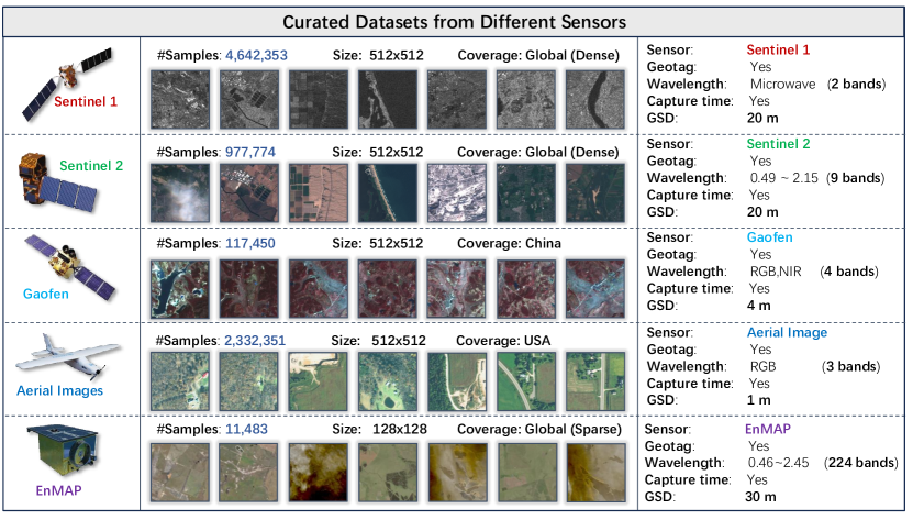
Figure S1: This figure shows the curated multimodal dataset. Five data modalities with different spatial resolutions and spectral bands are included, including the data from Sentinel 1, Sentinel 2, Gaofen, aerial images, and the EnMAP mission.

Downstream task datasets

We evaluate the pretrained models on 12 downstream tasks organized in GEO-Bench ³⁵. These datasets cover various applications and data modalities in EO, including six classification tasks and six segmentation tasks. In addition, we also compare DOFA with existing state-of-the-art models on the RESISC-45 dataset to evaluate the effectiveness of our model.

Classification datasets

m-bigearthnet is a multi-label land cover land use classification dataset covering Europe. The dataset contains 22,000 Sentinel-2 images with patch size 120$\times$120 pixels. Each image belongs to one or more categories from 43 classes.

m-so2sat is a local climate zone classification dataset. The dataset contains 21,964 Sentinel-1 and Sentinel-2 image pairs, covering 42 cities around the globe. Each image has a patch size of 32$\times$32 and belongs to one of 17 types of local climate zones.

m-brick-kiln is a binary scene classification dataset to detect brick kilns, a highly polluting informal industry common in Bangladesh. It contains 17,061 Sentinel-2 images, each with a patch size of 64$\times$64.

m-forestnet is a dataset for classifying the drivers of primary forest loss in Indonesia. The dataset contains 8,446 Landsat-8 images of size 332$\times$332, distributed into 12 classes.

m-eurosat is an EU-wide land cover land use classification dataset. It contains 4,000 Sentinel-2 images with a size of 64$\times$64 and includes ten land cover land use classes.

m-pv4ger is a dataset for detecting solar panels. It has both classification and segmentation versions. The classification version is a binary classification task with 13,812 high-resolution RGB images of size 320$\times$320 pixels and resolution 0.1 m.

Segmentation tasks

m-pv4ger-seg is the segmentation version of the m-pv4ger dataset for solar panel detection. It contains 3,806 high-resolution RGB images with size 320$\times$320 pixels.

m-chesapeake-landcover is a high-resolution land cover mapping dataset covering the contiguous US with seven land cover classes. The dataset contains 5,000 RGB-NIR images with 1 m resolution and 256$\times$256 pixels patch size.

m-cashew-plantation is a cashew mapping dataset covering a 120 km² area in Benin to characterize the expansion of cashew plantations. It contains 1,800 Sentinel-2 images with patch size 256$\times$256 pixels.

m-SA-crop-type is a dataset for crop type segmentation from Sentinel-2 images. It contains 5,000 256$\times$256 pixels images covering an area in Brandenburg, Germany, and an area in Western Cape, South Africa.

m-nz-cattle is a binary cow detection dataset from high-resolution aerial images. It contains 655 0.1 m resolution RGB images, each with size 500$\times$500.

m-NeonTree is a dataset for canopy crown detection and delineation in co-registered airborne RGB, LiDAR, and hyperspectral images. It contains 457 multimodal image pairs with size 400$\times$400 and resolution 0.1 m.

D. Training

Pretraining

In the proposed DOFA, we use the central wavelengths of each spectral band as input to the dynamic weight generator. We convert the wavelength values uniformly to micrometer units µm for each spectral band. For SAR images from Sentinel-1, the wavelength is uniquely larger than other bands, and therefore the µm unit is not reasonable. We thus set the $\lambda$ to 3.75 to distinguish it from different bands.

UPerNet ⁴¹ is used as the segmentation head for the segmentation-related downstream tasks. For all the models except the GFM with Swin Transformer, we transform the features into a feature pyramid with channels 512 and four different scales: (4, 2, 1, 0.5). Then the UPerNet segmentation head is used to output the segmentation results. More architecture details can be found in the code implementation.

We pretrain vision transformers (base and large) with patch size 16 on the collected multimodal pretraining dataset. We initiated pretraining for the baseline “MAE_Single” model using a subset of 50,000 images. For each of the five modalities, we randomly choose 10,000 samples. The DOFA models are pretrained progressively. Initially, we pretrained the DOFA models on the subset containing 50,000 images for 100 epochs. Subsequently, we further pretrained the models on an expanded set of 410,000 images over 20 epochs. During this phase, we select 100,000 samples from each of the Sentinel-1, Sentinel-2, Gaofen, and NAIP modalities. For hyperspectral images, we choose 10,000 samples from EnMAP data. Finally, we conduct a single epoch on the entire curated dataset to complete the training. We randomly crop and resize each image to 224$\times$224 as the input size to the ViT encoders. We normalize the images based on each modality’s mean and standard deviation. For the teacher models, we use the models of ViT-Base and ViT-Large pretrained on the ImageNet21K ⁸¹.

We adopt the masked image modeling design of MAE ³⁷ for self-supervised pretraining, which includes a regular ViT encoder and a lightweight ViT decoder. Only the encoder is transferred to downstream tasks. The masking ratio is set to 75%. We pretrain ViTs with a batch size of 128 for 100 epochs. We use the AdamW optimizer ⁸² with a weight decay of 0.05 and an initial learning rate of 1.5$e$-4. The learning rate is warmed up for 20 epochs and then decayed with a cosine schedule.

Transfer learning

We use the data loading tool of GEO-Bench ³⁵ to load the downstream datasets. We freeze the transferred encoder and train a linear classifier for classification tasks. Similarly, we freeze the encoder and train a UPerNet ⁴¹ decoder for segmentation tasks. For all the models except the GFM with Swin Transformer, we transform the features into a feature pyramid with channels 512 and four different scales: (4, 2, 1, 0.5). Then the UPerNet segmentation head is used to output the segmentation results. More architecture details can be found in the code implementation.

We follow the common practice of using RandomResizedCrop (scale 0.8 to 1.0) and RandomHorizontalFlip as data augmentations for classification tasks. The default crop size is 224$\times$224 for all datasets and baseline models except SatMAE ¹⁸ and CROMA ²⁰, of which the crop size is 96$\times$96 for SatMAE and 120$\times$120 for CROMA following the official setup to match their smaller patch size of 8. We use center crop, random rotation, and random horizontal and vertical flips for segmentation tasks. Images of each dataset are normalized based on the dataset’s mean and standard deviation.

We optimize cross-entropy loss for most datasets except m-bigearthnet, for which the MultiLabelSoftMarginLoss (or binary cross-entropy loss) is used. The LARS optimizer is utilized with cosine decay to train the last linear layer of each foundation model for 50 epochs. Considering the wide range of diversity among existing foundation models, we employ dataset-specific learning rates and batch sizes tailored to enhance the performance of classification tasks. We sweep over a grid search to pick the best learning rate from [0.5, 1.0, 10, 20] for each dataset. We use the AdamW optimizer, batch size 64, and an initial learning rate of 0.005 with cosine decay for 20 epochs for segmentation tasks. The learning rate is relatively stable across datasets for segmentation tasks.

E. Additional results

We visualize the accuracy curves of different SOTA models in Fig. S2 for the classification and segmentation datasets. These figures show that the proposed DOFA converges faster than other models on different datasets. A lower fine-tuning loss on downstream tasks suggests a higher adaptability of the foundation model to the specific dataset.

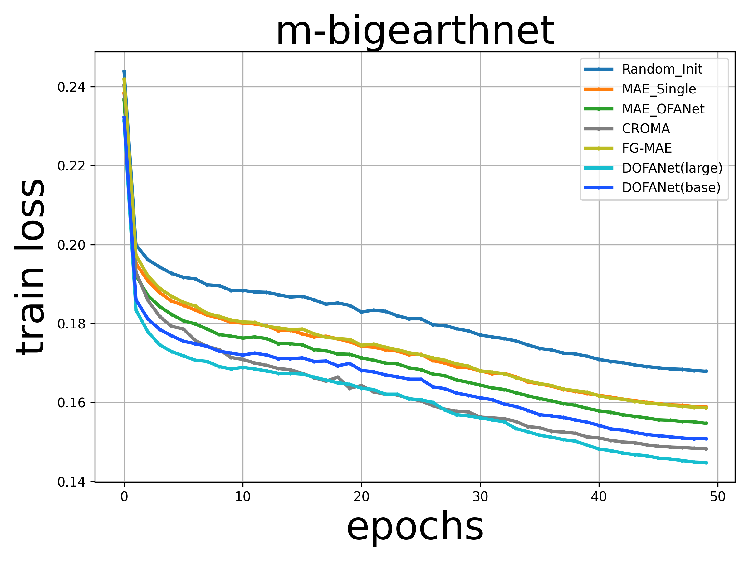
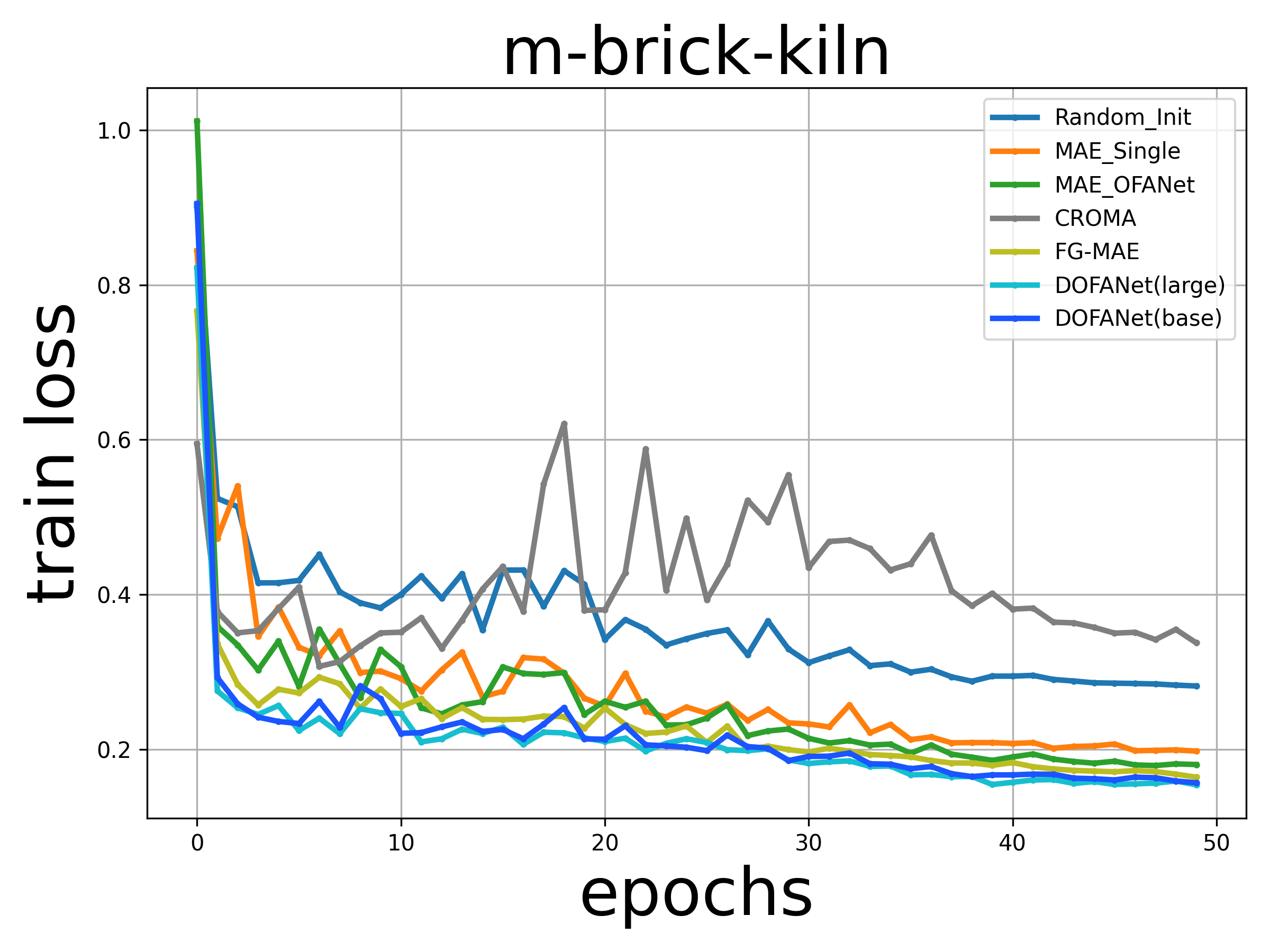
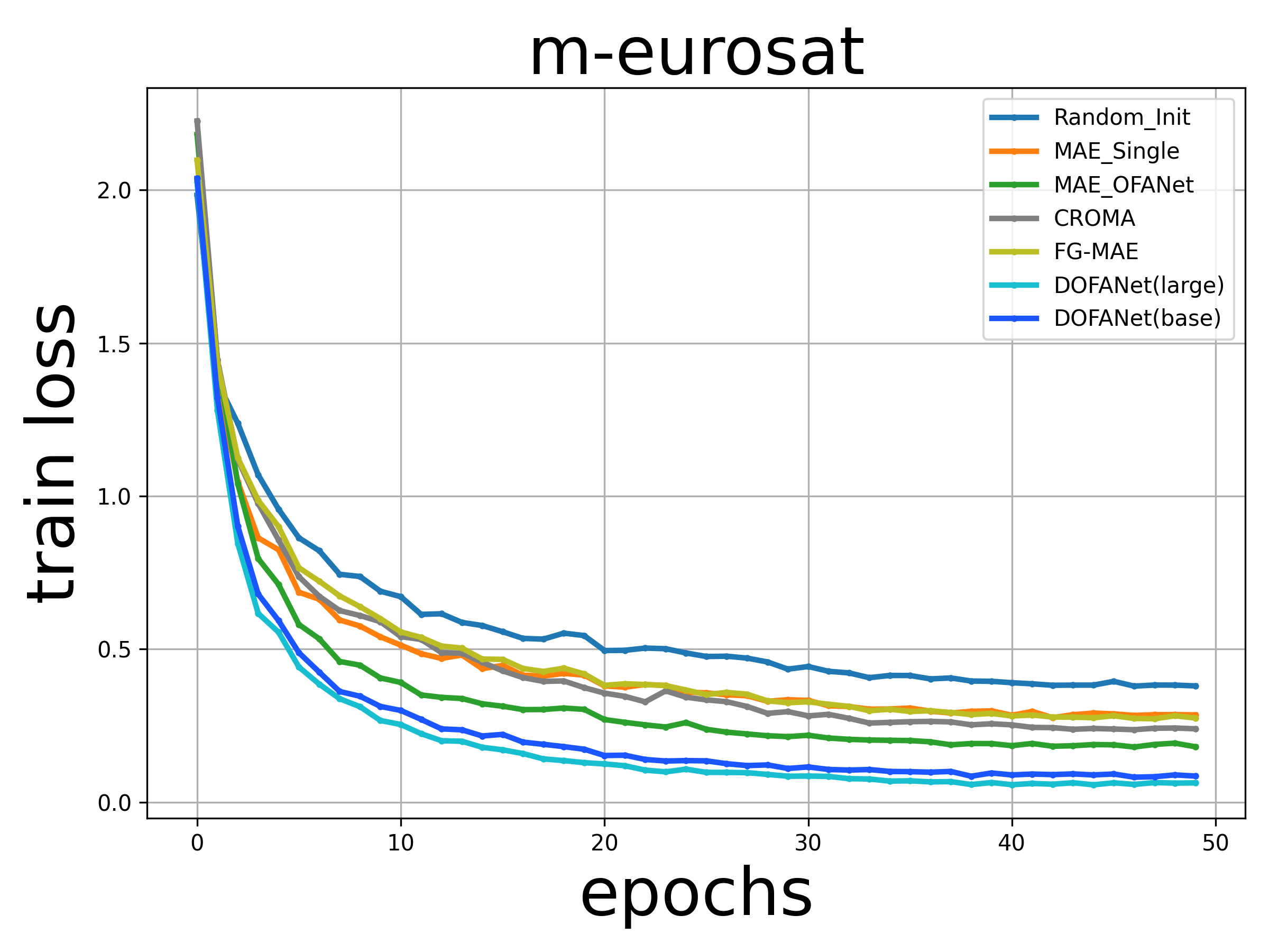
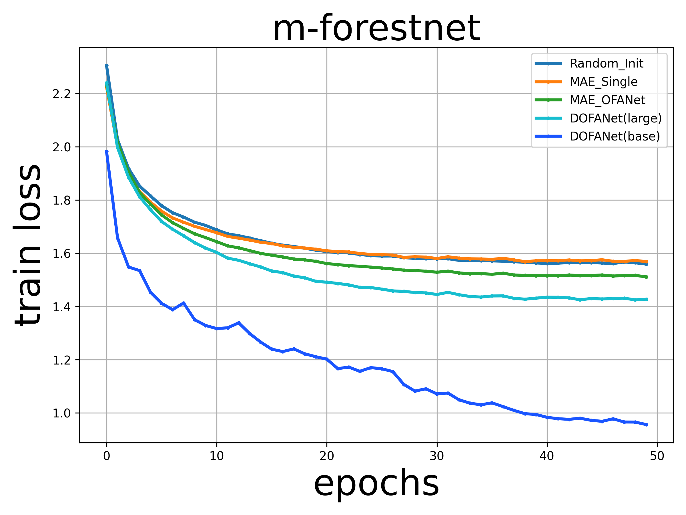
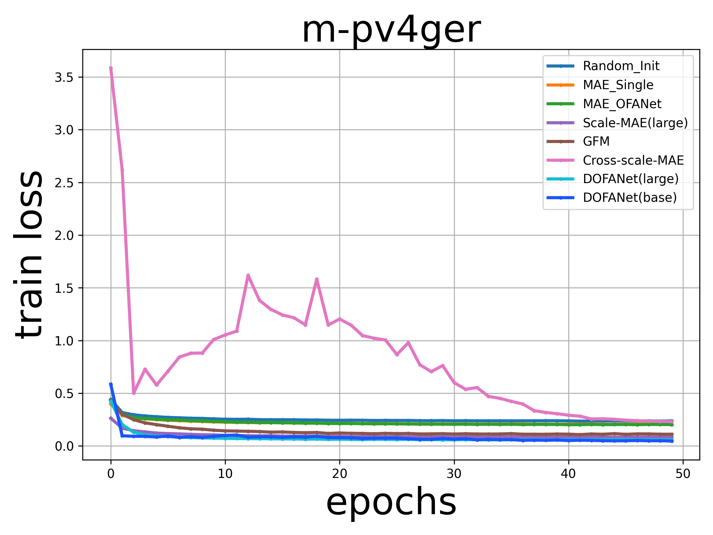
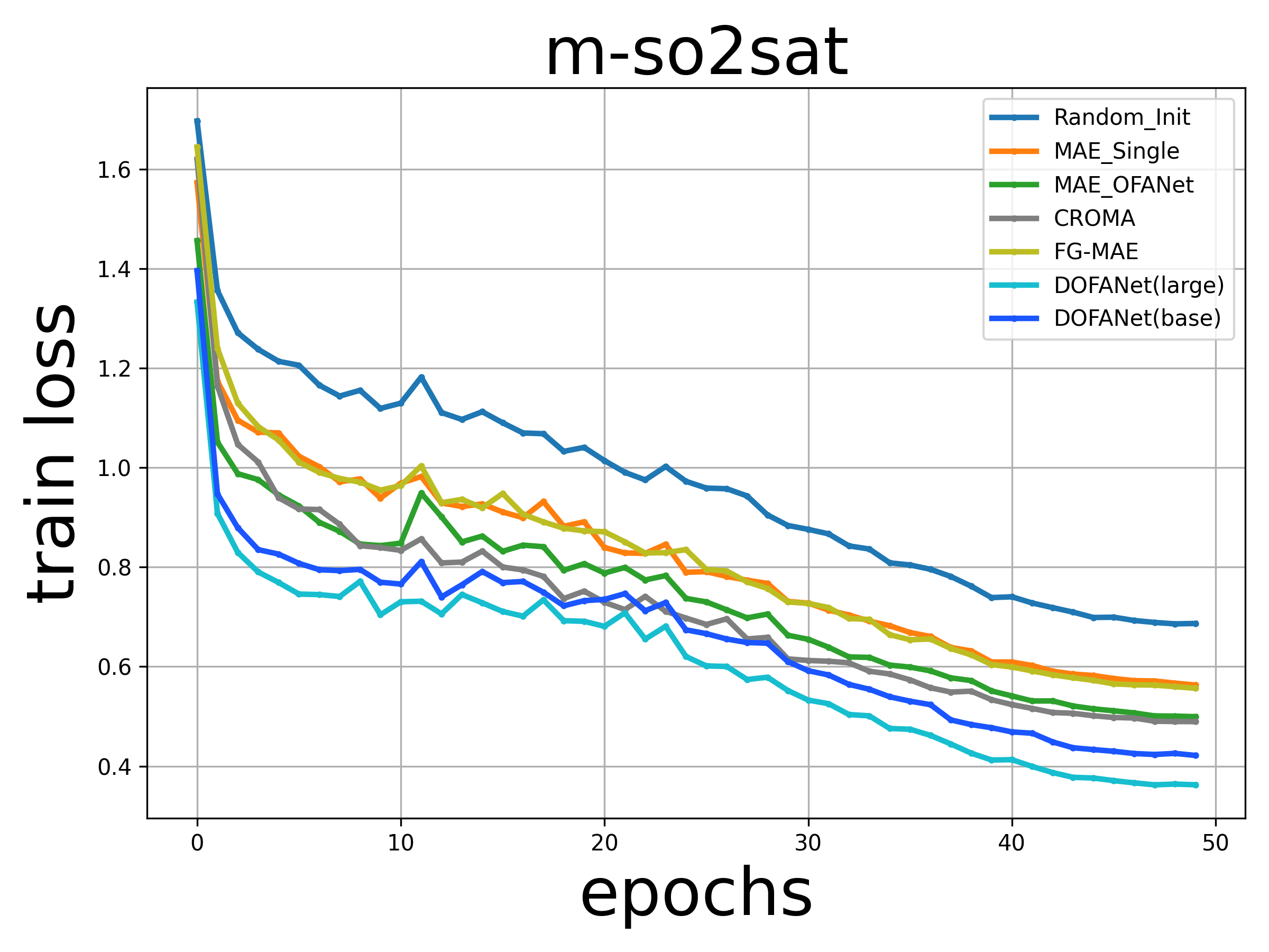
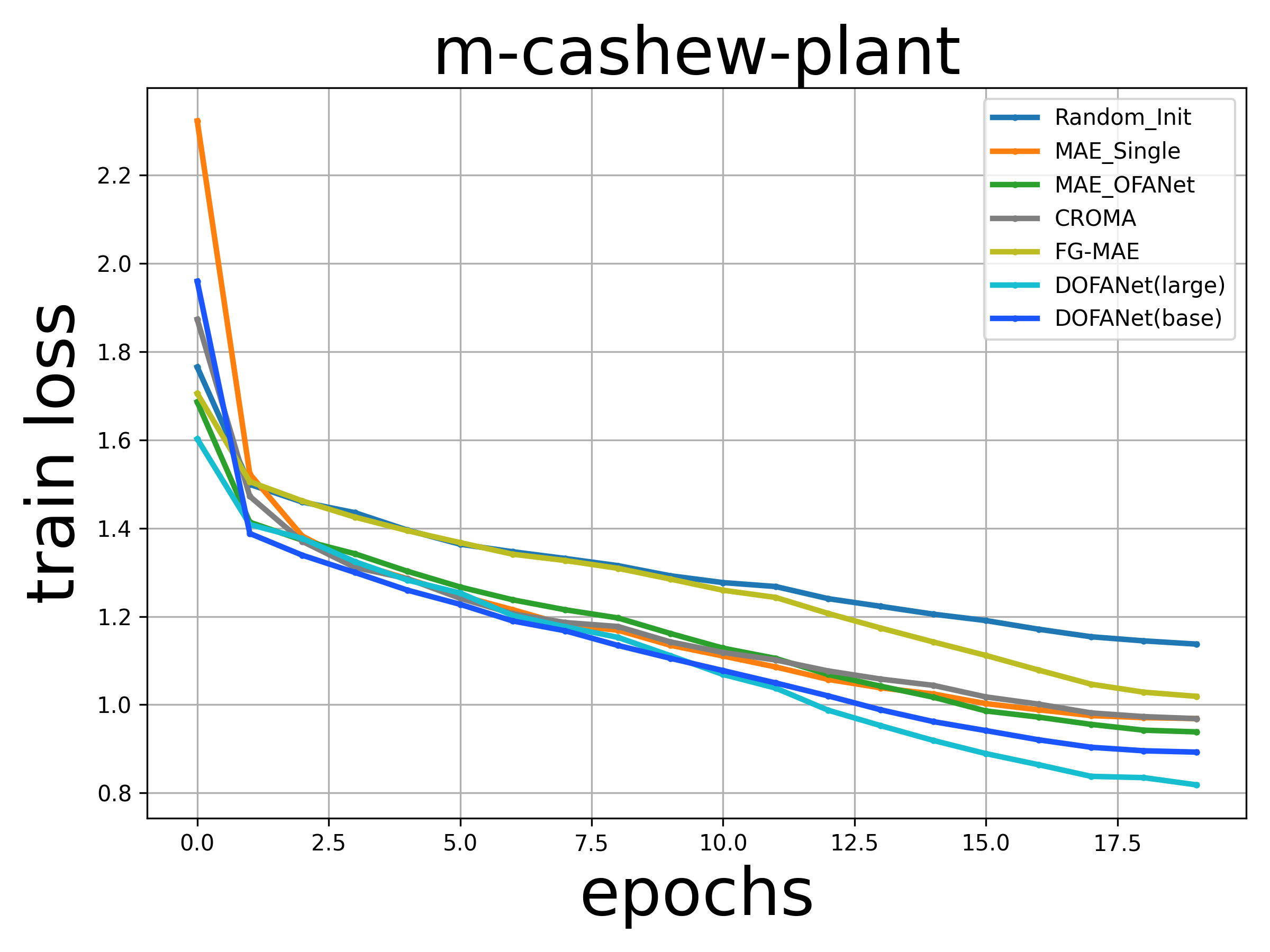
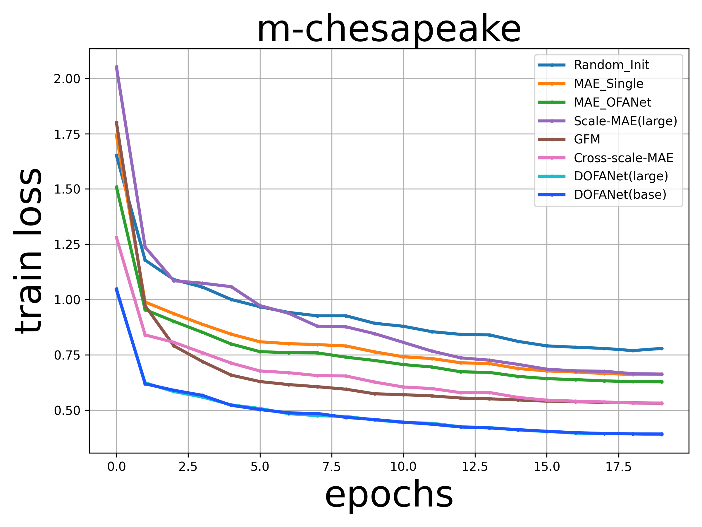
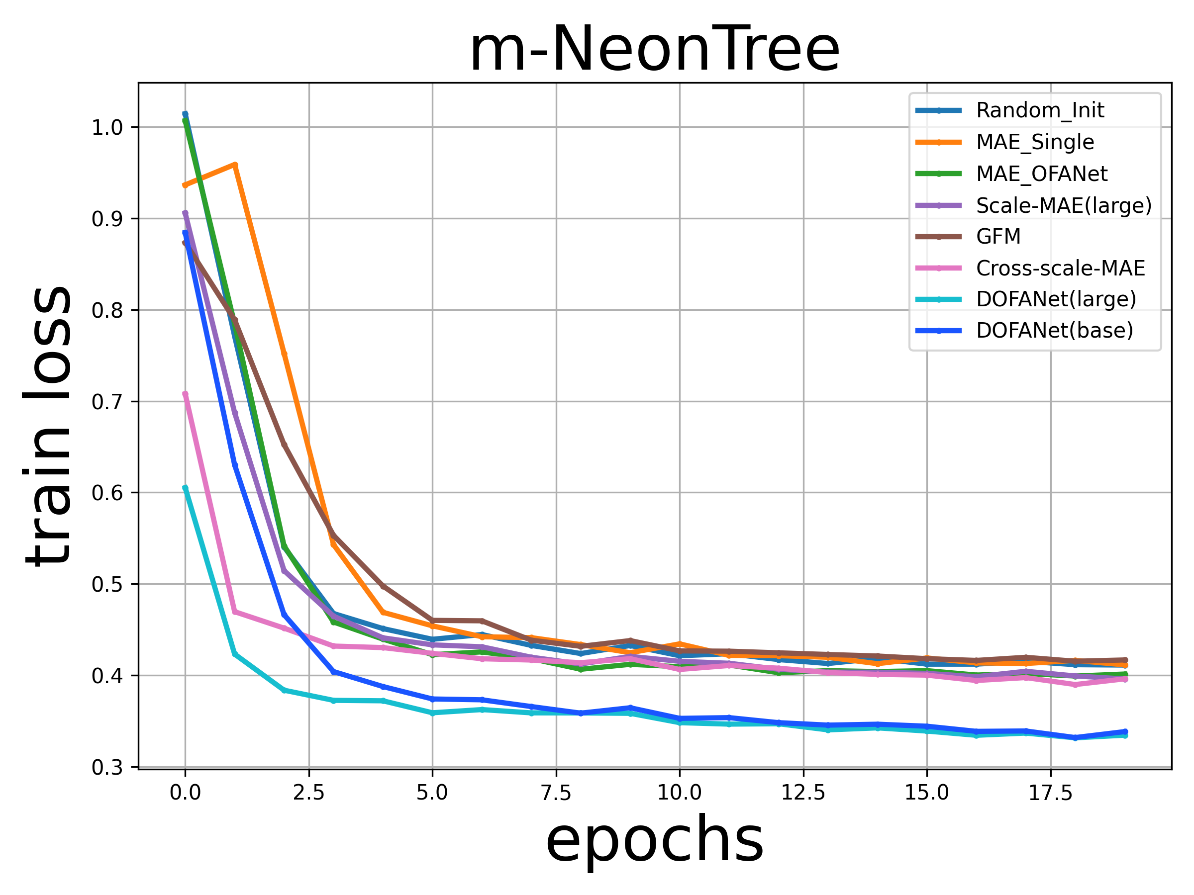
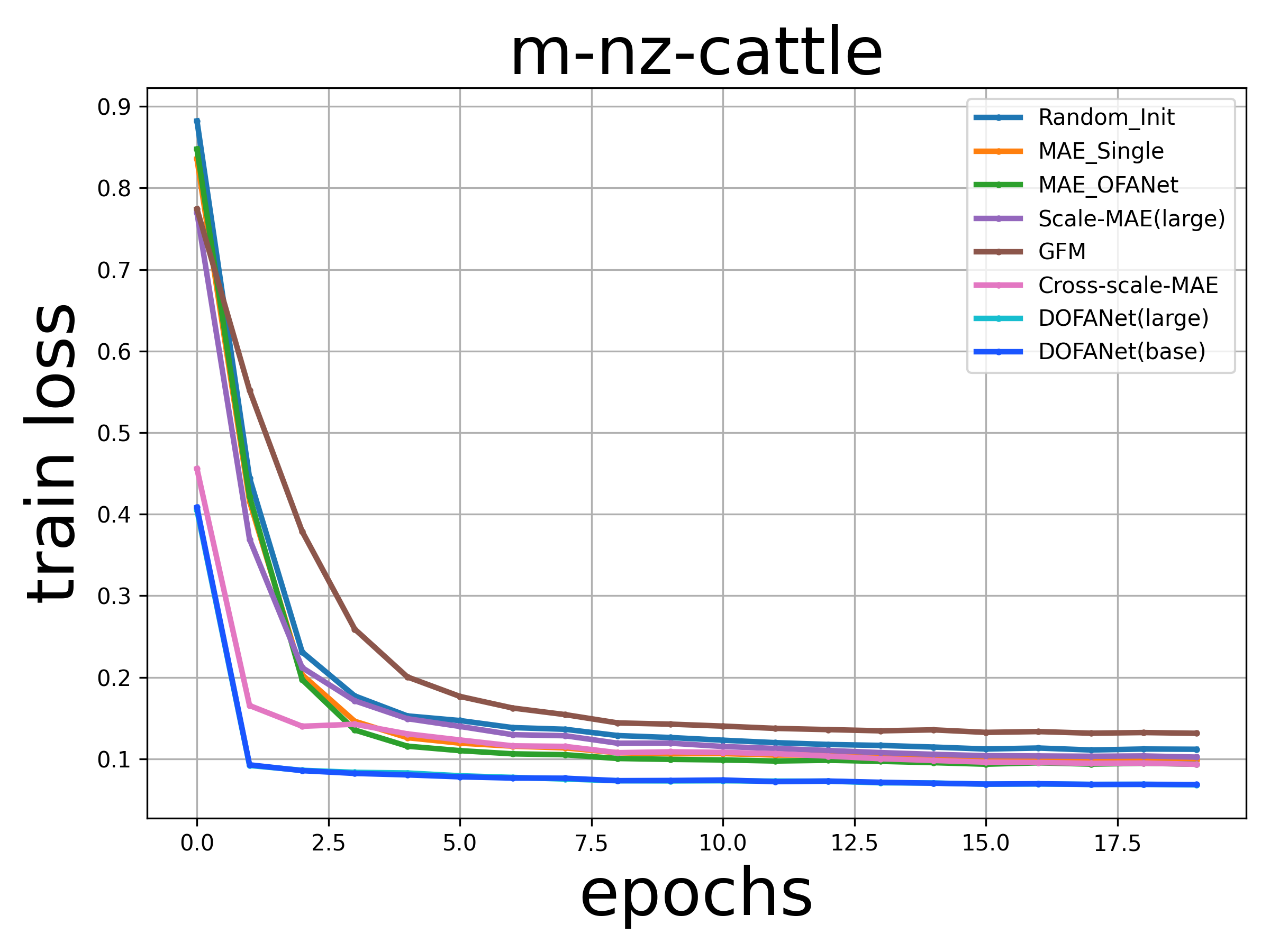
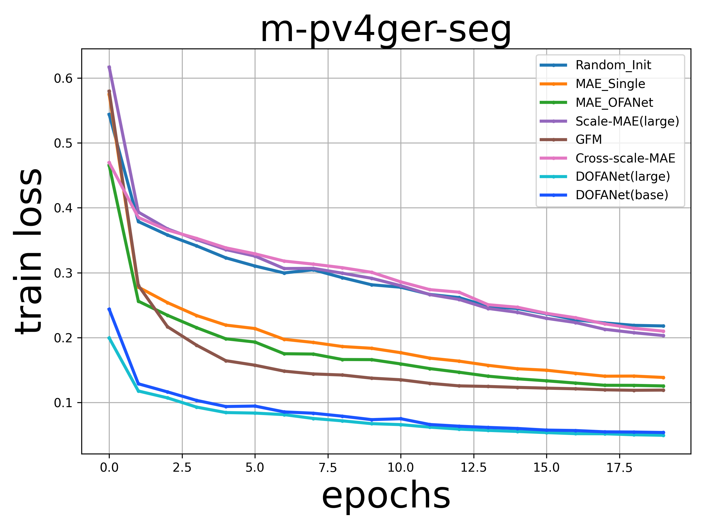
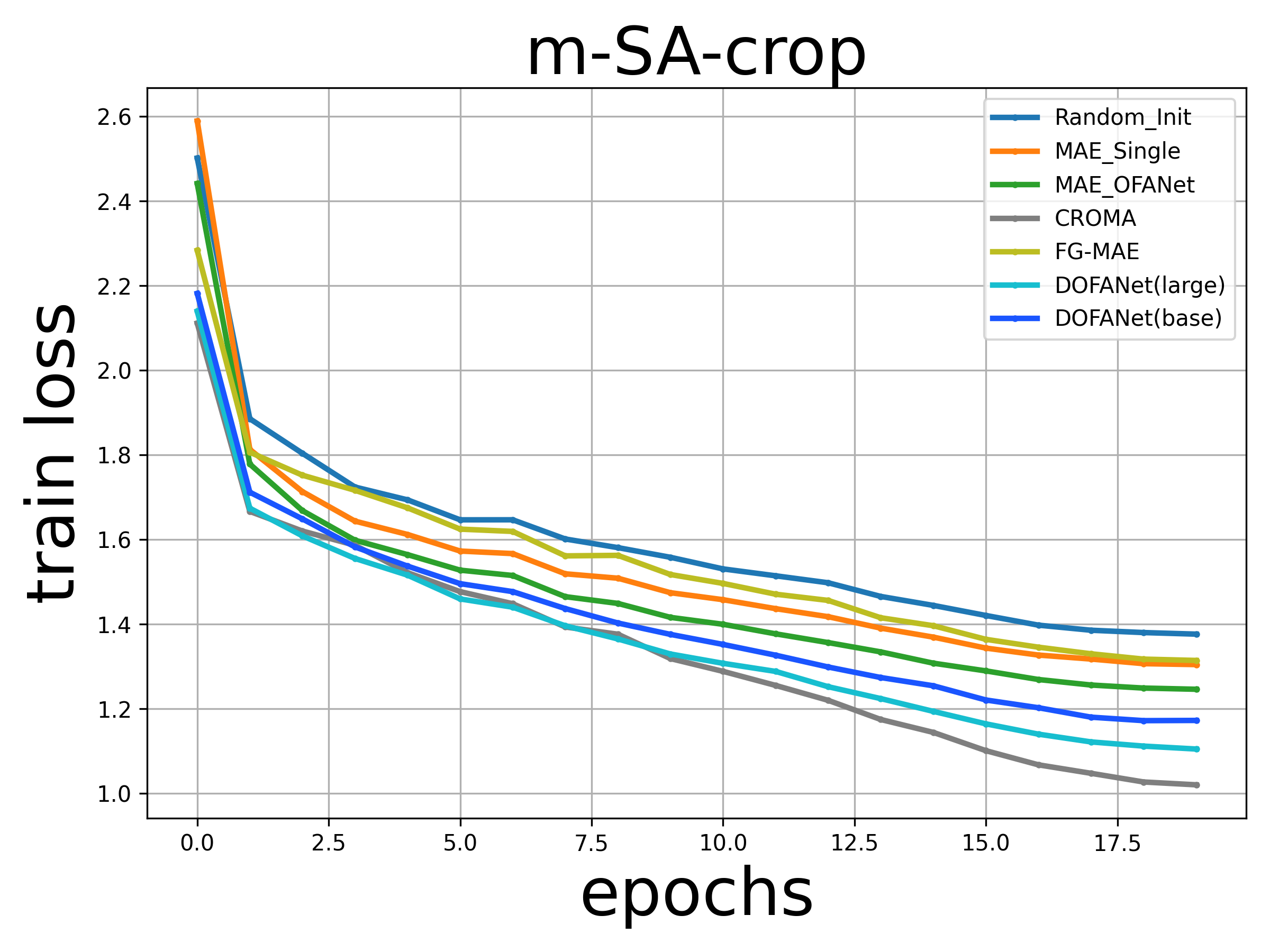
Figure S2: Visualization of the loss curves of different foundation models on the classification and segmentation datasets. It can be seen that the proposed DOFA converges faster than other models on these datasets.

F. Using the model and weights

The DOFA model and pre-trained weights are distributed via the TorchGeo library ⁸³. The pre-trained model can be easily instantiated using the following code.

⬇

import torch

from torchgeo.models import DOFABase16_Weights, dofa_base_patch16_224

# Example NAIP image (wavelengths in $\mu$m)

x = torch.rand(2, 4, 224, 224)

wavelengths = [0.48, 0.56, 0.64, 0.81]

# Use pre-trained model weights

model = dofa_base_patch16_224(weights=DOFABase16_Weights.DOFA_MAE)

# Make a prediction (model may need to be finetuned first)

y = model(x, wavelengths)

References

- \bibcommenthead
- Camps-Valls et al. 2011 Camps-Valls, G., Tuia, D., Gómez-Chova, L., Jiménez, S., Malo, J.: Remote sensing image processing (2011)
- Camps-Valls et al. 2021 Camps-Valls, G., Tuia, D., Zhu, X.X., Reichstein, M.: Deep learning for the Earth sciences: A comprehensive approach to remote sensing, climate science and geosciences (2021)
- Reichstein et al. 2019 Reichstein, M., Camps-Valls, G., Stevens, B., Jung, M., Denzler, J., Carvalhais, N., Prabhat: Deep learning and process understanding for data-driven Earth system science. Nature 566(7743), 195–204 (2019)
- Roy et al. 2014 Roy, D.P., Wulder, M.A., Loveland, T.R., Woodcock, C.E., Allen, R.G., Anderson, M.C., Helder, D., Irons, J.R., Johnson, D.M., Kennedy, R., et al.: Landsat-8: Science and product vision for terrestrial global change research. Remote Sensing of Environment 145, 154–172 (2014)
- Drusch et al. 2012 Drusch, M., Del Bello, U., Carlier, S., Colin, O., Fernandez, V., Gascon, F., Hoersch, B., Isola, C., Laberinti, P., Martimort, P., et al.: Sentinel-2: ESA’s optical high-resolution mission for GMES operational services. Remote Sensing of Environment 120, 25–36 (2012)
- Salomonson et al. 1989 Salomonson, V.V., Barnes, W., Maymon, P.W., Montgomery, H.E., Ostrow, H.: MODIS: Advanced facility instrument for studies of the Earth as a system. IEEE Transactions on Geoscience and Remote Sensing 27(2), 145–153 (1989)
- Guanter et al. 2015 Guanter, L., Kaufmann, H., Segl, K., Foerster, S., Rogass, C., Chabrillat, S., Kuester, T., Hollstein, A., Rossner, G., Chlebek, C., et al.: The EnMAP spaceborne imaging spectroscopy mission for Earth observation. Remote Sensing 7(7), 8830–8857 (2015)
- Huang et al. 2018 Huang, W., Sun, S., Jiang, H., Gao, C., Zong, X.: GF-2 satellite 1m/4m camera design and in-orbit commissioning. Chinese Journal of Electronics 27(6), 1316–1321 (2018)
- USDA Farm Service Agency (FSA) 2015 USDA Farm Service Agency (FSA): National Agriculture Imagery Program (NAIP). USDA Geospatial Data Gateway (2015)
- Zhu et al. 2017 Zhu, X.X., Tuia, D., Mou, L., Xia, G.-S., Zhang, L., Xu, F., Fraundorfer, F.: Deep learning in remote sensing: A comprehensive review and list of resources. IEEE Geoscience and Remote Sensing Magazine 5(4), 8–36 (2017)
- Schmitt et al. 2023 Schmitt, M., Ahmadi, S.A., Xu, Y., Taşkın, G., Verma, U., Sica, F., Hänsch, R.: There are no data like more data: Datasets for deep learning in Earth observation. IEEE Geoscience and Remote Sensing Magazine (2023)
- Xiong et al. 2022 Xiong, Z., Zhang, F., Wang, Y., Shi, Y., Zhu, X.X.: EarthNets: Empowering AI in Earth observation. arXiv preprint arXiv:2210.04936 (2022)
- Bommasani et al. 2021 Bommasani, R., Hudson, D.A., Adeli, E., Altman, R., Arora, S., Arx, S., Bernstein, M.S., Bohg, J., Bosselut, A., Brunskill, E., et al.: On the opportunities and risks of foundation models. arXiv preprint arXiv:2108.07258 (2021)
- Mendieta et al. 2023 Mendieta, M., Han, B., Shi, X., Zhu, Y., Chen, C.: Towards geospatial foundation models via continual pretraining. In: Proceedings of the IEEE/CVF International Conference on Computer Vision, pp. 16806–16816 (2023)
- Reed et al. 2023 Reed, C.J., Gupta, R., Li, S., Brockman, S., Funk, C., Clipp, B., Keutzer, K., Candido, S., Uyttendaele, M., Darrell, T.: Scale-MAE: A scale-aware masked autoencoder for multiscale geospatial representation learning. In: Proceedings of the IEEE/CVF International Conference on Computer Vision, pp. 4088–4099 (2023)
- Tang et al. 2024 Tang, M., Cozma, A., Georgiou, K., Qi, H.: Cross-Scale MAE: A tale of multiscale exploitation in remote sensing. Advances in Neural Information Processing Systems 36 (2024)
- Wang et al. 2023 Wang, Y., Hernández, H.H., Albrecht, C.M., Zhu, X.X.: Feature guided masked autoencoder for self-supervised learning in remote sensing. arXiv preprint arXiv:2310.18653 (2023)
- Cong et al. 2022 Cong, Y., Khanna, S., Meng, C., Liu, P., Rozi, E., He, Y., Burke, M., Lobell, D., Ermon, S.: SatMAE: Pre-training transformers for temporal and multi-spectral satellite imagery. Advances in Neural Information Processing Systems 35, 197–211 (2022)
- Stewart et al. 2024 Stewart, A., Lehmann, N., Corley, I., Wang, Y., Chang, Y.-C., Ait Ali Braham, N.A., Sehgal, S., Robinson, C., Banerjee, A.: SSL4EO-L: Datasets and foundation models for Landsat imagery. Advances in Neural Information Processing Systems 36 (2024)
- Fuller et al. 2023 Fuller, A., Millard, K., Green, J.R.: CROMA: Remote sensing representations with contrastive radar-optical masked autoencoders. arXiv preprint arXiv:2311.00566 (2023)
- Wang et al. 2023 Wang, Y., Albrecht, C.M., Braham, N.A.A., Liu, C., Xiong, Z., Zhu, X.X.: DeCUR: decoupling common & unique representations for multimodal self-supervision. arXiv preprint arXiv:2309.05300 (2023)
- Hong et al. 2024 Hong, D., Zhang, B., Li, X., Li, Y., Li, C., Yao, J., Yokoya, N., Li, H., Ghamisi, P., Jia, X., et al.: SpectralGPT: Spectral remote sensing foundation model. IEEE Transactions on Pattern Analysis and Machine Intelligence (2024)
- Bastani et al. 2023 Bastani, F., Wolters, P., Gupta, R., Ferdinando, J., Kembhavi, A.: SatlasPretrain: A large-scale dataset for remote sensing image understanding. In: Proceedings of the IEEE/CVF International Conference on Computer Vision, pp. 16772–16782 (2023)
- Hebb 2005 Hebb, D.O.: The organization of behavior: A neuropsychological theory (2005)
- Zucker and Regehr 2002 Zucker, R.S., Regehr, W.G.: Short-term synaptic plasticity. Annual Review of Physiology 64(1), 355–405 (2002)
- Dan and Poo 2004 Dan, Y., Poo, M.-m.: Spike timing-dependent plasticity of neural circuits. Neuron 44(1), 23–30 (2004)
- Pittenger and Duman 2008 Pittenger, C., Duman, R.S.: Stress, depression, and neuroplasticity: A convergence of mechanisms. Neuropsychopharmacology 33(1), 88–109 (2008)
- Dayan and Cohen 2011 Dayan, E., Cohen, L.G.: Neuroplasticity subserving motor skill learning. Neuron 72(3), 443–454 (2011)
- Buckmaster et al. 2002 Buckmaster, P.S., Zhang, G.F., Yamawaki, R.: Axon sprouting in a model of temporal lobe epilepsy creates a predominantly excitatory feedback circuit. Journal of Neuroscience 22(15), 6650–6658 (2002)
- Duman and Duman 2015 Duman, C.H., Duman, R.S.: Spine synapse remodeling in the pathophysiology and treatment of depression. Neuroscience Letters 601, 20–29 (2015)
- Lillicrap et al. 2020 Lillicrap, T.P., Santoro, A., Marris, L., Akerman, C.J., Hinton, G.: Backpropagation and the brain. Nature Reviews Neuroscience 21(6), 335–346 (2020)
- Zhang et al. 2023 Zhang, T., Cheng, X., Jia, S., Li, C.T., Poo, M.-m., Xu, B.: A brain-inspired algorithm that mitigates catastrophic forgetting of artificial and spiking neural networks with low computational cost. Science Advances 9(34), 2947 (2023)
- Ha et al. 2017 Ha, D., Dai, A.M., Le, Q.V.: Hypernetworks. In: ICLR 2017 (2017)
- Deng et al. 2009 Deng, J., Dong, W., Socher, R., Li, L.-J., Li, K., Fei-Fei, L.: ImageNet: A large-scale hierarchical image database. In: 2009 IEEE Conference on Computer Vision and Pattern Recognition, pp. 248–255 (2009). Ieee
- Lacoste et al. 2023 Lacoste, A., Lehmann, N., Rodriguez, P., Sherwin, E.D., Kerner, H., Lütjens, B., Irvin, J.A., Dao, D., Alemohammad, H., Drouin, A., et al.: GEO-Bench: Toward foundation models for Earth monitoring. arXiv preprint arXiv:2306.03831 (2023)
- Xiong et al. 2024 Xiong, Z., Wang, Y., Zhang, F., Zhu, X.X.: One for all: Toward unified foundation models for Earth vision. arXiv preprint arXiv:2401.07527 (2024)
- He et al. 2022 He, K., Chen, X., Xie, S., Li, Y., Dollár, P., Girshick, R.: Masked autoencoders are scalable vision learners. In: Proceedings of the IEEE/CVF Conference on Computer Vision and Pattern Recognition, pp. 16000–16009 (2022)
- Dosovitskiy et al. 2020 Dosovitskiy, A., Beyer, L., Kolesnikov, A., Weissenborn, D., Zhai, X., Unterthiner, T., Dehghani, M., Minderer, M., Heigold, G., Gelly, S., et al.: An image is worth 16x16 words: Transformers for image recognition at scale. arXiv preprint arXiv:2010.11929 (2020)
- Liu et al. 2021 Liu, Z., Lin, Y., Cao, Y., Hu, H., Wei, Y., Zhang, Z., Lin, S., Guo, B.: Swin transformer: Hierarchical vision transformer using shifted windows. In: Proceedings of the IEEE/CVF International Conference on Computer Vision, pp. 10012–10022 (2021)
- Liu et al. 2022 Liu, Z., Mao, H., Wu, C.-Y., Feichtenhofer, C., Darrell, T., Xie, S.: A ConvNet for the 2020s. In: Proceedings of the IEEE/CVF Conference on Computer Vision and Pattern Recognition, pp. 11976–11986 (2022)
- Xiao et al. 2018 Xiao, T., Liu, Y., Zhou, B., Jiang, Y., Sun, J.: Unified perceptual parsing for scene understanding. In: Proceedings of the European Conference on Computer Vision (ECCV), pp. 418–434 (2018)
- Cheng et al. 2017 Cheng, G., Han, J., Lu, X.: Remote sensing image scene classification: Benchmark and state of the art. Proceedings of the IEEE 105(10), 1865–1883 (2017)
- McInnes et al. 2018 McInnes, L., Healy, J., Melville, J.: UMAP: Uniform manifold approximation and projection for dimension reduction. arXiv preprint arXiv:1802.03426 (2018)
- Van der Maaten and Hinton 2008 Maaten, L., Hinton, G.: Visualizing data using t-SNE. Journal of Machine Learning Research 9(11) (2008)
- Agarap 2018 Agarap, A.F.: Deep learning using rectified linear units (ReLU). arXiv preprint arXiv:1803.08375 (2018)
- Vaswani et al. 2017 Vaswani, A., Shazeer, N., Parmar, N., Uszkoreit, J., Jones, L., Gomez, A.N., Kaiser, Ł., Polosukhin, I.: Attention is all you need. Advances in Neural Information Processing Systems 30 (2017)
- Zhang et al. 2017 Zhang, L., Xiang, T., Gong, S.: Learning a deep embedding model for zero-shot learning. In: Proceedings of the IEEE Conference on Computer Vision and Pattern Recognition, pp. 2021–2030 (2017)
- Sung et al. 2018 Sung, F., Yang, Y., Zhang, L., Xiang, T., Torr, P.H., Hospedales, T.M.: Learning to compare: Relation network for few-shot learning. In: Proceedings of the IEEE Conference on Computer Vision and Pattern Recognition, pp. 1199–1208 (2018)
- Xiong et al. 2022 Xiong, Z., Li, H., Zhu, X.X.: Doubly deformable aggregation of covariance matrices for few-shot segmentation. In: European Conference on Computer Vision, pp. 133–150 (2022). Springer
- Liu et al. 2024 Liu, H., Li, C., Wu, Q., Lee, Y.J.: Visual instruction tuning. Advances in Neural Information Processing Systems 36 (2024)
- Touvron et al. 2023 Touvron, H., Lavril, T., Izacard, G., Martinet, X., Lachaux, M.-A., Lacroix, T., Rozière, B., Goyal, N., Hambro, E., Azhar, F., et al.: LLaMA: Open and efficient foundation language models. arXiv preprint arXiv:2302.13971 (2023)
- Brown et al. 2020 Brown, T., Mann, B., Ryder, N., Subbiah, M., Kaplan, J.D., Dhariwal, P., Neelakantan, A., Shyam, P., Sastry, G., Askell, A., et al.: Language models are few-shot learners. Advances in Neural Information Processing Systems 33, 1877–1901 (2020)
- OpenAI 2023 OpenAI: ChatGPT (June 26 version) [large language model] (2023). https://chat.openai.com/chat
- Radford et al. 2021 Radford, A., Kim, J.W., Hallacy, C., Ramesh, A., Goh, G., Agarwal, S., Sastry, G., Askell, A., Mishkin, P., Clark, J., et al.: Learning transferable visual models from natural language supervision. In: International Conference on Machine Learning, pp. 8748–8763 (2021). PMLR
- Li et al. 2022 Li, J., Li, D., Xiong, C., Hoi, S.: BLIP: Bootstrapping language-image pre-training for unified vision-language understanding and generation. In: International Conference on Machine Learning, pp. 12888–12900 (2022). PMLR
- Rombach et al. 2021 Rombach, R., Blattmann, A., Lorenz, D., Esser, P., Ommer, B.: High-resolution image synthesis with latent diffusion models (2021)
- Kirillov et al. 2023 Kirillov, A., Mintun, E., Ravi, N., Mao, H., Rolland, C., Gustafson, L., Xiao, T., Whitehead, S., Berg, A.C., Lo, W.-Y., et al.: Segment anything. arXiv preprint arXiv:2304.02643 (2023)
- Grill et al. 2020 Grill, J.-B., Strub, F., Altché, F., Tallec, C., Richemond, P., Buchatskaya, E., Doersch, C., Avila Pires, B., Guo, Z., Gheshlaghi Azar, M., et al.: Bootstrap your own latent: A new approach to self-supervised learning. Advances in Neural Information Processing Systems 33, 21271–21284 (2020)
- Caron et al. 2021 Caron, M., Touvron, H., Misra, I., Jégou, H., Mairal, J., Bojanowski, P., Joulin, A.: Emerging properties in self-supervised vision transformers. In: Proceedings of the IEEE/CVF International Conference on Computer Vision, pp. 9650–9660 (2021)
- Chen et al. 2020 Chen, T., Kornblith, S., Norouzi, M., Hinton, G.: A simple framework for contrastive learning of visual representations. In: International Conference on Machine Learning, pp. 1597–1607 (2020). PMLR
- Frome et al. 2013 Frome, A., Corrado, G.S., Shlens, J., Bengio, S., Dean, J., Ranzato, M., Mikolov, T.: DeViSE: A deep visual-semantic embedding model. Advances in Neural Information Processing Systems 26 (2013)
- Ye et al. 2019 Ye, L., Rochan, M., Liu, Z., Wang, Y.: Cross-modal self-attention network for referring image segmentation. In: Proceedings of the IEEE/CVF Conference on Computer Vision and Pattern Recognition, pp. 10502–10511 (2019)
- Lu et al. 2022 Lu, J., Clark, C., Zellers, R., Mottaghi, R., Kembhavi, A.: Unified-IO: A unified model for vision, language, and multi-modal tasks. arXiv preprint arXiv:2206.08916 (2022)
- Zou et al. 2023 Zou, X., Dou, Z.-Y., Yang, J., Gan, Z., Li, L., Li, C., Dai, X., Behl, H., Wang, J., Yuan, L., et al.: Generalized decoding for pixel, image, and language. In: Proceedings of the IEEE/CVF Conference on Computer Vision and Pattern Recognition, pp. 15116–15127 (2023)
- Zhang et al. 2023 Zhang, Y., Gong, K., Zhang, K., Li, H., Qiao, Y., Ouyang, W., Yue, X.: Meta-transformer: A unified framework for multimodal learning. arXiv preprint arXiv:2307.10802 (2023)
- Manas et al. 2021 Manas, O., Lacoste, A., Giró-i-Nieto, X., Vazquez, D., Rodriguez, P.: Seasonal contrast: Unsupervised pre-training from uncurated remote sensing data. In: Proceedings of the IEEE/CVF International Conference on Computer Vision, pp. 9414–9423 (2021)
- Mall et al. 2023 Mall, U., Hariharan, B., Bala, K.: Change-aware sampling and contrastive learning for satellite images. In: Proceedings of the IEEE/CVF Conference on Computer Vision and Pattern Recognition, pp. 5261–5270 (2023)
- Cha et al. 2023 Cha, K., Seo, J., Lee, T.: A billion-scale foundation model for remote sensing images. arXiv preprint arXiv:2304.05215 (2023)
- Yao et al. 2023 Yao, F., Lu, W., Yang, H., Xu, L., Liu, C., Hu, L., Yu, H., Liu, N., Deng, C., Tang, D., et al.: RingMo-sense: Remote sensing foundation model for spatiotemporal prediction via spatiotemporal evolution disentangling. IEEE Transactions on Geoscience and Remote Sensing (2023)
- Irvin et al. 2023 Irvin, J., Tao, L., Zhou, J., Ma, Y., Nashold, L., Liu, B., Ng, A.Y.: USat: A unified self-supervised encoder for multi-sensor satellite imagery. arXiv preprint arXiv:2312.02199 (2023)
- Wang et al. 2023 Wang, Y., Braham, N.A.A., Xiong, Z., Liu, C., Albrecht, C.M., Zhu, X.X.: SSL4EO-S12: A large-scale multimodal, multitemporal dataset for self-supervised learning in Earth observation. IEEE Geoscience and Remote Sensing Magazine 11(3), 98–106 (2023)
- Ayush et al. 2021 Ayush, K., Uzkent, B., Meng, C., Tanmay, K., Burke, M., Lobell, D., Ermon, S.: Geography-aware self-supervised learning. In: Proceedings of the IEEE/CVF International Conference on Computer Vision, pp. 10181–10190 (2021)
- Cepeda et al. 2023 Cepeda, V.V., Nayak, G.K., Shah, M.: GeoCLIP: Clip-inspired alignment between locations and images for effective worldwide geo-localization. arXiv preprint arXiv:2309.16020 (2023)
- Klemmer et al. 2023 Klemmer, K., Rolf, E., Robinson, C., Mackey, L., Rußwurm, M.: SatCLIP: Global, general-purpose location embeddings with satellite imagery. arXiv preprint arXiv:2311.17179 (2023)
- Guo et al. 2023 Guo, X., Lao, J., Dang, B., Zhang, Y., Yu, L., Ru, L., Zhong, L., Huang, Z., Wu, K., Hu, D., et al.: SkySense: A multi-modal remote sensing foundation model towards universal interpretation for Earth observation imagery. arXiv preprint arXiv:2312.10115 (2023)
- Jean et al. 2019 Jean, N., Wang, S., Samar, A., Azzari, G., Lobell, D., Ermon, S.: Tile2Vec: Unsupervised representation learning for spatially distributed data. In: Proceedings of the AAAI Conference on Artificial Intelligence, vol. 33, pp. 3967–3974 (2019)
- Christie et al. 2018 Christie, G., Fendley, N., Wilson, J., Mukherjee, R.: Functional map of the world. In: Proceedings of the IEEE Conference on Computer Vision and Pattern Recognition, pp. 6172–6180 (2018)
- Wang et al. 2022 Wang, Y., Braham, N.A.A., Xiong, Z., Liu, C., Albrecht, C.M., Zhu, X.X.: SSL4EO-S12: A large-scale multi-modal, multi-temporal dataset for self-supervised learning in Earth observation. arXiv preprint arXiv:2211.07044 (2022)
- Tong et al. 2023 Tong, X.-Y., Xia, G.-S., Zhu, X.X.: Enabling country-scale land cover mapping with meter-resolution satellite imagery. ISPRS Journal of Photogrammetry and Remote Sensing 196, 178–196 (2023)
- Fuchs and Demir 2023 Fuchs, M.H.P., Demir, B.: HySpecNet-11k: A large-scale hyperspectral dataset for benchmarking learning-based hyperspectral image compression methods. arXiv preprint arXiv:2306.00385 (2023)
- Steiner et al. 2021 Steiner, A., Kolesnikov, A., Zhai, X., Wightman, R., Uszkoreit, J., Beyer, L.: How to train your ViT? data, augmentation, and regularization in vision transformers. arXiv preprint arXiv:2106.10270 (2021)
- Loshchilov and Hutter 2017 Loshchilov, I., Hutter, F.: Decoupled weight decay regularization. arXiv preprint arXiv:1711.05101 (2017)
- Stewart et al. 2022 Stewart, A.J., Robinson, C., Corley, I.A., Ortiz, A., Lavista Ferres, J.M., Banerjee, A.: TorchGeo: Deep learning with geospatial data. In: Proceedings of the 30th International Conference on Advances in Geographic Information Systems. SIGSPATIAL ’22, pp. 1–12. Association for Computing Machinery, Seattle, Washington (2022). https://doi.org/10.1145/3557915.3560953
Acknowledgments
The work of Z.X., F.Z., Y.W., F.Z., A.J.S., and X.X.Z is jointly supported by the German Federal Ministry of Education and Research (BMBF) in the framework of the international future AI lab “AI4EO – Artificial Intelligence for Earth Observation: Reasoning, Uncertainties, Ethics and Beyond” (grant number: 01DD20001), by German Federal Ministry for Economic Affairs and Climate Action in the framework of the “national center of excellence ML4Earth” (grant number: 50EE2201C), by the German Federal Ministry for the Environment, Nature Conservation, Nuclear Safety and Consumer Protection (BMUV) based on a resolution of the German Bundestag (grant number: 67KI32002B; Acronym: EKAPEx) and by Munich Center for Machine Learning. The work of Z. X., I.P., G.C.V., and X. X. Z is also funded by the European Commission through the project “ThinkingEarth—Copernicus Foundation Models for a Thinking Earth” under the Horizon 2020 Research and Innovation program (Grant Agreement No. 101130544). GCV was partly funded by the European Research Council (ERC) Synergy Grant “Understanding and Modeling the Earth System with Machine Learning” (USMILE) under the Horizon 2020 Research and Innovation program (Grant Agreement No. 855187).