Guided Decoding for Robot Motion Generation and Adaption

Abstract

We address motion generation for high-DoF robot arms in complex settings with obstacles, via points, etc. A significant advancement in this domain is achieved by integrating Learning from Demonstration (LfD) into the motion generation process. This integration facilitates rapid adaptation to new tasks and optimizes the utilization of accumulated expertise by allowing robots to learn and generalize from demonstrated trajectories.

We train a transformer architecture on a large dataset of simulated trajectories. This architecture, based on a conditional variational autoencoder transformer, learns essential motion generation skills and adapts these to meet auxiliary tasks and constraints. Our auto-regressive approach enables real-time integration of feedback from the physical system, enhancing the adaptability and efficiency of motion generation. We show that our model can generate motion from initial and target points, but also that it can adapt trajectories in navigating complex tasks, including obstacle avoidance, via points, and meeting velocity and acceleration constraints, across platforms.

I Introduction

Motion generation is a challenging topic for robot arms with high degrees of freedom (DoF). One main challenge is to generate smooth motion trajectories to solve a given task while ensuring the robot and its environment’s safety, and respecting the robot’s embodiment constraints. This problem is especially complex when the task involves auxiliary objectives beyond reaching a target point, such as avoiding obstacles, passing via specified points, or imposing velocity or acceleration constraints. Another particularly intriguing aspect of motion generation is the incorporation of learning from demonstration (LfD) within the same process. Allowing users or agents to present a guiding trajectory based on prior knowledge helps the rapid development of robotic applications. This capability is crucial for adapting to novel tasks and leveraging accumulated expertise effectively. Motion primitives offer a promising avenue for achieving this goal [1, 2, 3, 4]. By encapsulating fundamental motion behaviors into primitives, the robot can learn and generalize from demonstrations, promoting versatility and adaptability in complex tasks. Integrating learning from demonstration with the challenges of motion generation presents an exciting direction for advancing the capabilities of robot arms with high degrees of freedom.

In this work, we propose a framework for learning motion generation. We create a large dataset of robot motion trajectories with multiple simulated robots and train a transformer architecture to learn to generate motion based on given initial and target points. We design a Transformer conditional variational autoencoder. The trained generative model encapsulates basic motion generation skills based on the training data. We further propose an approach to efficiently adapt the generated motion to satisfy auxiliary tasks and constraints such as obstacle avoidance, via points and velocity constraints. The whole process is auto-regressive allowing for integrating feedback from the real system during motion generation. Our approach allows for generating motion based on an initial and target point only, or to imitate a full trajectory given by a user or external agent. Our experiments show the usability of our method for motion generation, under via point constraints, obstacles, and velocity and acceleration constraints. We also show the benefits of training with data collected using various robots. Additionally, we show the ability to imitate and adapt user-given trajectories to a given task.

II Methods

In this section, we present a Transformer-based autoencoder model in Sec. II-A to II-C, followed by an introduction to adaptation methods based on an autoregressive decoder in Section II-D and II-E (see Fig. 1).

II-A Inference model for the infilling task

We consider a dataset $\mathcal{D}=\{x^{(i)}\}^{N}_{i=1}$ of trajectories $x^{(i)}=\{x^{(i)}_{t}\}_{t=1}^{T}$ and our goal is to learn representations that can help us generate new trajectories given a starting point $x_{1}$ and an endpoint $x_{T}$. We propose to do this with the Conditional VAE [5] model

$$p_{\theta}(x_{2:T-1}|x_{1,T})=\int p_{\theta}(x_{2:T-1}|x_{1,T},z)\>p_{\theta}(z|x_{1,T})\,dz$$

where the latent variables $z$ are expected to encode latent features of paths with starting point $x_{1}$ and endpoint $x_{T}$. We learn this by minimizing the negative ELBO

$$L(\theta,\phi)= -\mathrm{E}_{\hat{p}(x_{1:T})}\mathrm{E}_{q_{\phi}(z;x_{1:T})}[\log p_{\theta}(x_{2:T-1}|x_{1,T},z)]$$

$$+\mathrm{E}_{\hat{p}(x_{1:T})}\mathrm{KL}[q_{\phi}(z;x_{1:T})\,\|\,p_{\theta}(z;x_{1,T})].$$

Here $p_{\theta}(z|x_{1,T})$ is the conditional prior model, $p_{\theta}(x_{2:T-2}|x_{1,T},z)$ is the decoder/generation model, and $q_{\phi}(z|\operatorname{x}_{1:T})$ is the encoder/recognition model. To generate a trajectory, we sample the latent of the decoder input $z\sim p_{\theta}(z|x_{1,T})$. We then sample with an auto-regressive decoder $p_{\theta}(x^{\prime}_{t+1}|x^{\prime}_{2:t},x_{1,T},z)$. The training process can be found in App. -A.

Either the prior or the autoregressive decoder is capable of generating diverse samples. To enhance adaptability and generalization, our model incorporates both for distinct purposes. With a fixed demonstration/posterior, we can adjust the trajectories from the decoder. Conversely, by specifying a starting and ending point, we can generate various trajectories using the prior.

II-B PerceiverIO encoder

We implement the encoder $q_{\phi}(\operatorname{z}|\operatorname{x}_{1:T})$ via a PerceiverIO model [6], that is, as multi-layered, attention-based neural architecture where each layer is composed of a cross-attention (CA) and as self-attention (SA) block as

$$h^{(l+1)}_{1:K} =\mathrm{RMLP}_{\theta}\circ\mathrm{RSA}_{\theta}(h_{1:K}^{(l)}),\quad l=1,\ldots,L$$

$$h^{(1)}_{1:K} =\mathrm{RMLP}_{\theta}\circ\mathrm{RCA}_{\theta}(h^{(0)}_{1:K},\tilde{x}_{1:T}).$$

The initial layer $h^{(0)}_{\theta}$ is a learned parameter, a part of $\theta$. The values $\tilde{x}_{t}=W_{\theta}x_{t}+\tau_{t}$ are embedding the data into the hidden space via a linear layer $W_{\theta}$ and a positional embedding $\tau_{t}$. RCA and RSA denote a residual (R) cross-attention and residual self-attention block defined as $\mathrm{RCA}(h,z)=\mathrm{LayerNorm}(h+\mathrm{CA}(h,z))$ and $\mathrm{RSA}(h)=\mathrm{LayerNorm}(h+\mathrm{SA}(h))$, respectively. The encoder is then defined as a diagonal multivariate Gaussian distribution $q_{\phi}(z|x_{1:T})=\mathcal{N}(z;\mu_{\theta}^{\mathrm{enc}}(h^{(L)}),\sigma_{\theta}^{\mathrm{enc}}(h^{(L)})^{2})$ with $\mu_{\theta}^{\mathrm{enc}}$ and $\sigma_{\theta}^{\mathrm{enc}}$ being simple MLPs. The latent variable $z$ is thus designed to encode the trajectory $x_{1:T},x_{t}\in\mathbb{R}^{d}$ to a shorter sequence of $K$ variables $z_{k}\in\mathbb{R}^{m}$. Note that the choice $K=1$ results in a single vector embedding of the trajectory $x_{1:T}$.

To implement the prior $p_{\theta}(z|x_{1,T})$ we use the same model having as input only the pair $\{x_{1},x_{T}\}$.

This type of Perceiver architecture is designed to reduce the quadratic ($T\times T$) computational complexity of a Transformer encoder model (self-attention layers) on $x_{1:T}$ by only cross-attending the sequence ($T\times K$) and performing less computationally demanding self-attentions ($K\times K$) on $z_{1:K}$. Generally, there is a large class of Perceiver models/blocks with learnable queries or latents that are used for transforming data between different modalities, for example, a Perceiver model with $K$ queries can be used as a head-block in a classification model with $K$ classes.

II-C Autoregressive decoder

Figure 1: Model overview. Each PerceiverIO module gets a trajectory, but for the prior it only contains the beginning and end points and a full trajectory for the posterior. During training, minimizing the KL divergence between the two makes the representation of the PerceiverIO module that only gets $x_{1}$ and $x_{T}$ generates the same latent distribution as the one getting the full trajectory; therefore, it learns interpolation. The latent state then is used by the autoregressive decoder to generate the next setpoint $x_{t+1}$. Dashed lines indicate components used exclusively during the post-training adaptation phase, not included in the initial training process.

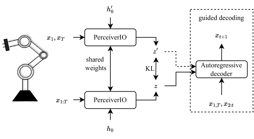
A natural choice for the decoder in the context of attention-based models is a conditional autoregressive model

$$p_{\theta}(x_{2:T-1}|x_{1,T},z)=\prod_{t=1}^{T-1}p_{\theta}(x_{t+1}|x_{2:t},x_{1,T},z).$$

Here, we again use an attention-based neural architecture, a standard transformer decoder [7] defined as

$$h^{(l)}_{1:T}=\mathrm{RMLP}^{(l+1)}_{\theta}\circ\mathrm{RCA}_{\theta}^{(l+1)}(\cdot,z)\circ\mathrm{RCSA}_{\theta}^{(l+1)}(h^{(l)}_{1:T})$$

with $h^{(0)}_{1:T}=\tilde{x}_{1:T}$ being the embeddings defined in the previous section. The value $h^{(L)}_{t}$ is then used to define the autoregressive model $p(x_{t+1}|x_{2:t},x_{1,T},z)=\mathcal{N}(x_{t+1};\mu_{\theta}^{\mathrm{dec}}(h^{(L)}_{t}),\sigma_{\theta}^{\mathrm{dec}}(h^{(L)}_{t})^{2})$. The additional “C” in the layer definition in $\mathrm{RCSA}$ denotes a casual attention model implemented via triangular attention masks. Unlike Transformers for text infilling [8, 9], we do not include segmentation embedding since the length and position of the start and end points in the model are already provided.

II-D Trajectory generator—Guided decoding

In addition to learning a conditional autoencoder model for trajectory generation we would also like to extend the model to be able to perform online trajectory adaptation, for example, add via-points and obstacle avoidance. To achieve this we do online (approximate) probabilistic inference using $p_{\theta}(x_{t+1}|x_{1:t},x_{T},z)$ without updating the model parameter $\theta$. The obvious choice is a Bayesian approach where the adaptation can be formulated as a Bayesian update of $p_{\theta}(x_{t+1}|x_{1:t},x_{T},z)$, via a likelihood $p(y_{t+1}|x_{t+1})$. Alternatively, the likelihood can also be used to implement constraints, for example, a Bayesian update with a likelihood function $\mathrm{I}_{[a,b]}(x)$ can implement trajectory boundaries.

For generic constraints we can formulate online trajectory adaptation as

$$\min_{q(x_{t+1})} \>\mathrm{KL}[q(x_{t+1})\,\|\,p_{\theta}(x_{t+1}|x_{1:t},x_{T},z)]$$ (1)

$$\mathrm{s.t.} \>\mathrm{E}_{q(x_{t+1})}[H(c(x_{t+1}))]\leq\alpha,$$ (2)

where $H(\cdot)$ is the Heaviside function, $c(\cdot)$ is a constraint function. The constraint in (2) expresses what proportion $0\leq\alpha\leq 1$ of the probability mass is allowed not to satisfy the constraint [10]. The KL objective is convex in $q$, the constraints are linear, and the optimal solution $(q^{\ast},\lambda^{\ast})$ satisfies

$$q^{\ast}(x_{t+1})\propto p_{\theta}(x_{t+1}|x_{1:t},x_{T},z)\times\exp\{-\lambda^{\ast}H(c(x_{t+1}))\}.$$

Solving this optimization, however, even for as Gaussian $q$ and a $c$ implementing a boundary constraint can be numerically demanding. For more general constraints such as obstacle avoidance, (2) can be analytically intractable. For this reason, in the following we will only exploit the form of $q^{\ast}(x_{t+1})$ to propose fast online trajectory adaptation methods. Various trajectory adaptations can be conveniently formulated either as (1) by choosing the appropriate constraint function $c(\cdot)$ or as a Bayesian update with the appropriate likelihood. These will be detailed in the following.

II-E Implementing specific constraints

II-E1 Obstacle avoidance with beam search

Beam search (BS) [11] is a classic heuristic in the field of natural language processing (autoregressive models). It is used to generate trajectories with high likelihood or other specific score values. The method recursively generates trajectories as follows. A set of $S$ trajectories $\{x_{2:t}^{(s)}\}$ are stored together with their scores, for example, the path likelihood $\log p(x_{2:t}^{(s)}|x_{1,T},z)$. For each trajectory $S$ new samples $x_{t+1}^{(s,r)}\sim p(x_{t+1}|x_{2:t}^{(s)},x_{1,T},z),r=1,\ldots,S$ are generated as candidates and the corresponding total scores are computed for the extended trajectories $(x^{(s)}_{2:t},x_{t+1}^{(s,r)})$ for all $(s,r)$ pairs. The overall top $S$ extended trajectories are selected for the next step. Inspired by the form of $q^{\ast}(x_{t+1})$, we define the score by adding $\tilde{s}(x_{t+1})=-\gamma\max(c(x_{t+1}),0)$ with $c(x)=\delta^{2}-\|\,x-x_{\mathrm{obstacle}}\,\|^{2}$ to the likelihood.

II-E2 Position, velocity and acceleration bounds

Simple position and velocity bounds in an interval $[a,b]$ can be implemented via a Bayesian update. In case of position bounds the posterior, $q(x_{t+1})\propto\mathrm{I}_{[a,b]}(x_{t+1})\>p_{\theta}(x_{t+1}|x_{1:t},x_{T},z)$ is a truncated Gaussian from which we can easily sample. In case of velocity bounds $[v_{\mathrm{min}},v_{\mathrm{max}}]$, we notice that $v_{t}=(x_{t+1}-x_{t})/{\Delta t}$ is Gaussian to which we can apply a Bayesian update via $\mathrm{I}_{[v_{\mathrm{min}},v_{\mathrm{max}}]}(v_{t})$. Due to the fact that the predictive distribution is a diagonal (independent) Gaussian, this results in a truncated Gaussian distribution on $v_{t+1}$ and subsequently on $x_{t+1}$. Acceleration bounds follow the same principle applied to $a_{t}=(\operatorname{x}_{t+1}-2x_{t}+x_{t-1})/{\Delta t^{2}}$.

II-E3 Via points through Brownian bridge

To add additional via-points to the autoregressive model $p_{\theta}(x_{t+1}|x_{1:t},x_{T},z)$, say, $x_{s}$ at an intermediate time $1<s<T$ we would have to compute the Bayesian posterior

$$p(x_{t+1} |x_{1:t},x_{s},x_{T},z)$$

$$\propto p(x_{s}|x_{t+1},x_{1:t},x_{T},z)\times p(x_{t+1}|x_{1:t},x_{T},z).$$

Since the likelihood term $p(x_{s}|x_{t+1},x_{1:t},x_{T},z)$ is intractable, we propose to approximate it with a Gaussian likelihood

$$p(x_{s}|x_{t+1},x_{1:t},x_{T},z)\approx\mathcal{N}(x_{s}|x_{t+1},(s-t-1)\>\sigma_{\mathrm{vp}}^{2}).$$

To have a stronger conditioning on the past $x_{1:t}$ we can alternatively use a Brownian-bridge approximation

$$\mathcal{N}\left(x_{t+1}|x_{t}+\frac{1}{s-t}(x_{s}-x_{t}),\sigma^{2}_{\mathrm{vp}}\frac{s-t-1}{s-t}\right).$$

Both of the above approximations lead to a Gaussian approximation of $p(x_{t+1}|x_{1:t},x_{s},x_{T},z)$.

II-E4 Constrained Beam Search for Brownian bridge

Drawing on the Constrained Beam Search (CBS) described by [12], we refine the approach by integrating a controller. This addition drives the generated trajectory towards the desired outcome, rather than substituting words.

We generate samples of $x_{t+1}$ for each sample $x_{t}$, using the Transformer decoder incorporating via point method, i.e., Brownian Bridge. We categorize the generated trajectories into three banks: Bank0 for trajectories that do not meet the constraint; Bank1 for trajectories that have applied the controller but still do not satisfy the constraint; and Bank2 for trajectories that satisfy the constraint. For the trajectory $x_{1:t}$ that satisfies the via-point constraint, we generate a single sample of $x_{t+1}$ using the Transformer decoder exclusively for Bank2. If $x_{1:t}$ fails to satisfy the constraint, we then generate one $x_{t+1}$ sample from the Transformer decoder with the controller. In this case, if $x_{t+1}$ satisfies the constraint, the sample is allocated to Bank2; otherwise, it goes to Bank1. Lastly, in cases where $x_{1:t}$ does not satisfy the constraint, we generate $N_{s}$ $x_{t+1}$ samples from the Transformer decoder only. Here, if $x_{t+1}$ satisfies, the sample is classified into Bank2; if not, into Bank0. Following this, we select the samples from each bank with the order of Bank2, Bank1, Bank0, iteratively based on the negative log-likelihood criterion until we have $N_{s}$ samples in total for $x_{t+1}$.

Previous work [12] has demonstrated that CBS outperforms BS during guided language generation, akin to via point task in robot trajectory generation. However, for tasks such as obstacle avoidance, only BS is applicable, since Bank0 and Bank1 cannot be defined.

III Related work

In robotics, movement primitives are used to specify behavior based on human-demonstrated trajectories. Dynamic movement primitives (DMP) take inspiration from dynamical systems to specify motion behavior [1, 2]. DMPs use human demonstrations to fit a forcing term that augments the attractor dynamics to match the demonstrated trajectories. DMPs allow motion adaptation, such as avoidance of obstacles, by adding additional terms such as repulsive fields to their driving equation [13, 14]. This process should be done carefully to avoid competing objectives. Furthermore, DMPs applied in latent space [15, 16] provide the capability to adjust motions within this latent space. Unlike these works which adapt the latent space incrementally, our approach is a sequence-to-sequence model. In our model, each trajectory is mapped to a distinct point in the latent space, affording greater flexibility in guiding the decoder’s output. Probabilistic movement primitives represent trajectory distributions, which simplifies the blending of multiple trajectories [3]. Adapting movement to auxiliary tasks is also possible within this framework [10, 17, 18]. Riemannian motion policies easily allow the combination of multiple behaviors in both the task and the configuration space [4]. However, this method lacks the advantages of probabilistic formulations.

IV Experiments

IV-A Data Collection

To train our models we collect a large dataset of robot motion trajectories in simulation. We use the NVIDIA IsaacSim simulator to generate a large amount of data in parallel. Our main experiments are based on data using the Franka Emika Panda robot. However, for the multi-robot experiment we also introduce motion data from different robots, namely Rethink Robotic’s Sawyer, Kuka’s LBR IIWA 7, Jaco and Kinova Gen3 from Kinova Robotics, and Universal Robot’s UR5e. We generate samples for each robot in 4096 environments in parallel and repeat this process for multiple episodes. At the beginning of each episode, we randomly sample starting and end-goal positions in the configuration space. We then use a proportional derivative controller to drive the robot to the goal position. To generate more diverse trajectories, we occasionally sample via points at the beginning of an episode and use these as target points for a short while at the beginning of the episode.

For the trajectory of the end-effector, we have $x\in\mathbb{R}^{3}$, while $x\in\mathbb{R}^{7}$ for joint space. The robots which have 6-DOF are padded zero to match this representation. Each sequence has a total length of $T=64$.

IV-B Distances to the original trajectories

Figure 2: Distances to the original trajectories for the Panda robot in Cartesian space.

Figure 3: Distances to the original trajectories for IIWA robot in joint space.

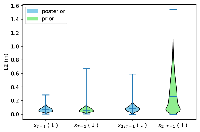
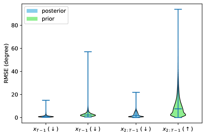
We split the dataset into 20,000 training, 2048 validation, and 2048 test samples. A single robot was trained and then evaluated on its performance. Fig. 2 and 3 illustrate the generalization from the prior and the reconstruction. Evaluation metrics include the Root Mean Square Error (RMSE) measured in degrees for joint movements, and an L2 Norm, measured in meters, for assessing the trajectories for the end-effector. Assuming endpoint distances are the same, a larger distance for trajectories from the prior distribution to the original demos is advantageous, as it demonstrates the diversity of the learned prior. Except that, lower distance values to the original samples indicate better performance, where the distance reflects the fidelity of the model’s output approximating the original trajectories. Rather than determining the endpoint distance, we calculate the distance at $x_{T-1}$, since the $x_{T}$ is given.

IV-C Generalization on an unknown robot

Figure 4: Distances to the original trajectories for the Panda robot in Cartesian space with multiple-robot training and single-robot training.

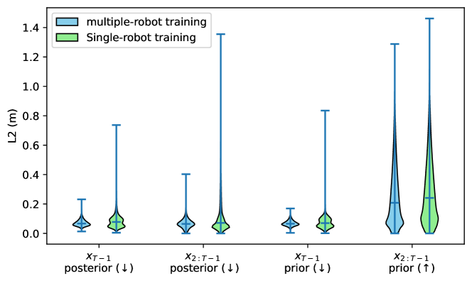
Scaling up models across various robots presents significant challenges but offers substantial benefits, as noted in [19]. To assess our model’s ability to generalize, we conducted an experiment involving different robots. In this experiment, the training dataset comprises IIWA, UR5e, and Sawyer robots operating in Cartesian space. The validation dataset uses the Jaco robot, while the Panda robot is the test dataset. For comparison of single-robot training, the training dataset was divided into three subsets, each corresponding to a specific robot, with the same validation and test datasets used across all experiments. The results from the single-robot training are aggregated for presentation. As illustrated in Fig. 4, training across multiple robots demonstrates superior generalization to an unknown robot.

IV-D Adaptation and generalization

The experiments are trained on a Panda robot. Our adaption and generalization are suitable for both samples from priors and posterior. To enhance visualization and compare with demonstrations, we present all results based on samples from posteriors, except for those in Sections IV-D2 and IV-D4 which also use samples from priors.

IV-D1 Via points

Figure 5: Brownian bridge for via point with (upper) and without (lower) CBS. Colors indicate the axes of the Cartesian coordinate.

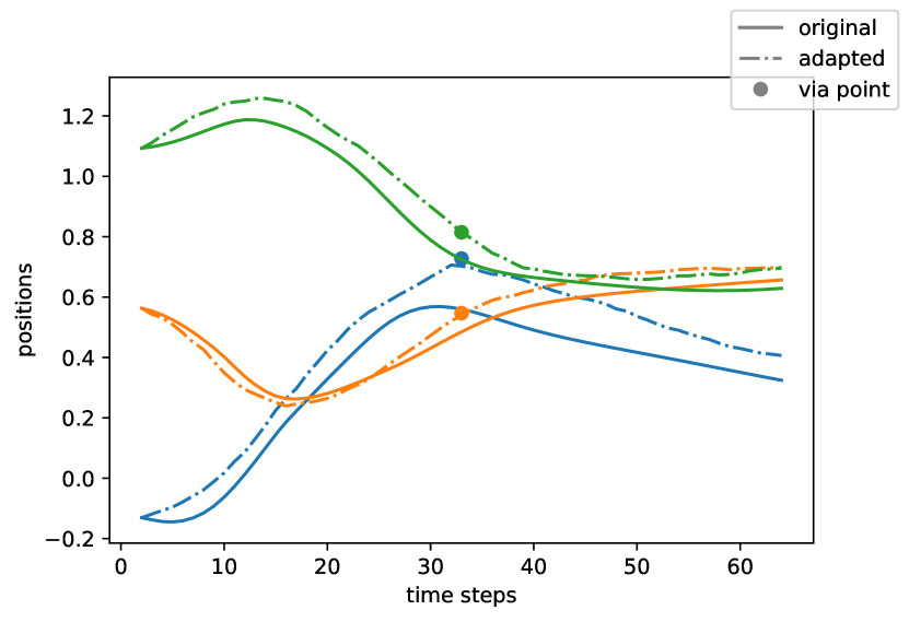
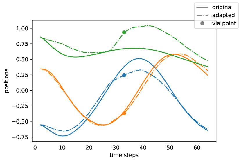
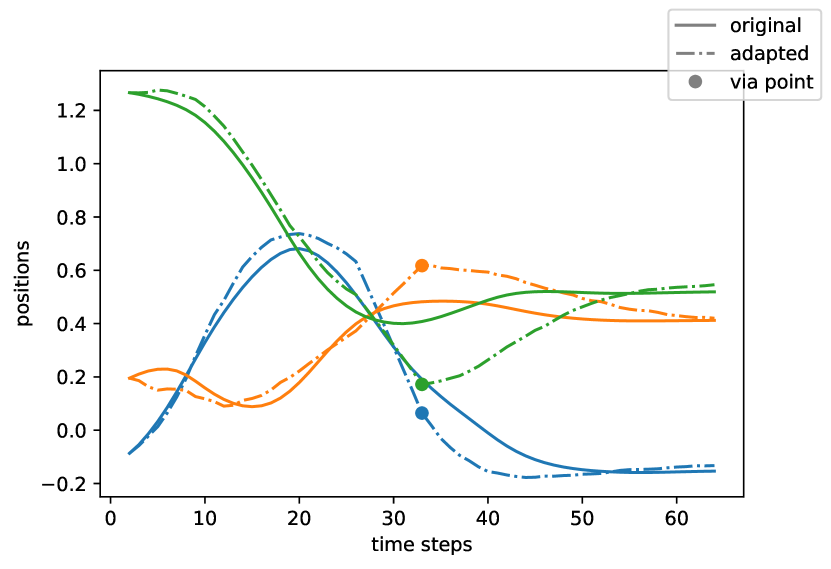
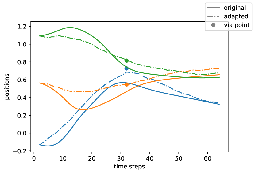
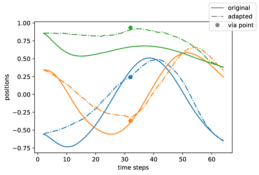
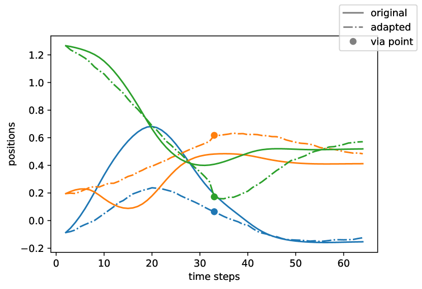
We adapted the movements for via point (see Fig. 5) using the Brownian bridge. We set the hyperparameter $\sigma_{\mathrm{vp}}$ in a similar range of the output $\sigma$ from the autoregressive decoder. The experiments show the comparisons between via points without and with CBS, where the beam search size is set to five. The findings indicate that when CBS is used, the trajectories appear more natural and closer to the original demos. On the contrary, as CBS is a historical search method, a Brownian bridge without CBS enables online trajectory generation.

IV-D2 Obstacle avoidance

Figure 6: Adaption for obstacle avoidance. (Upper) Obstacle avoidance with the samples from the posterior. (Lower) Obstacle avoidance with samples from the prior, where the original refers to the samples from the prior without adaptation of the decoder. All of them successfully avoid the obstacles, although the visualization is not perfect due to the viewpoint.

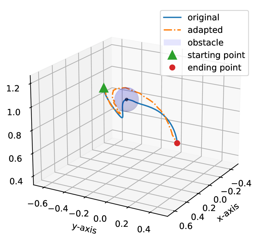
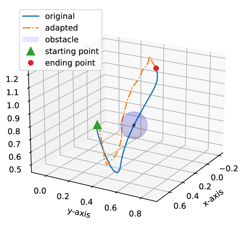
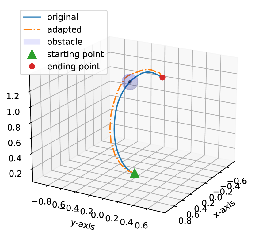
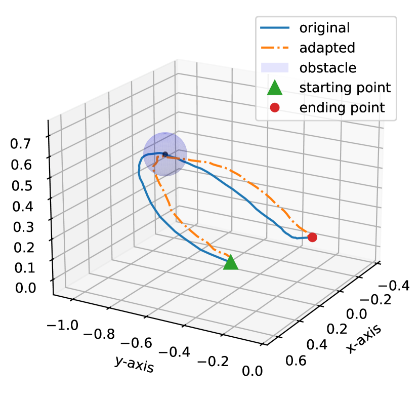
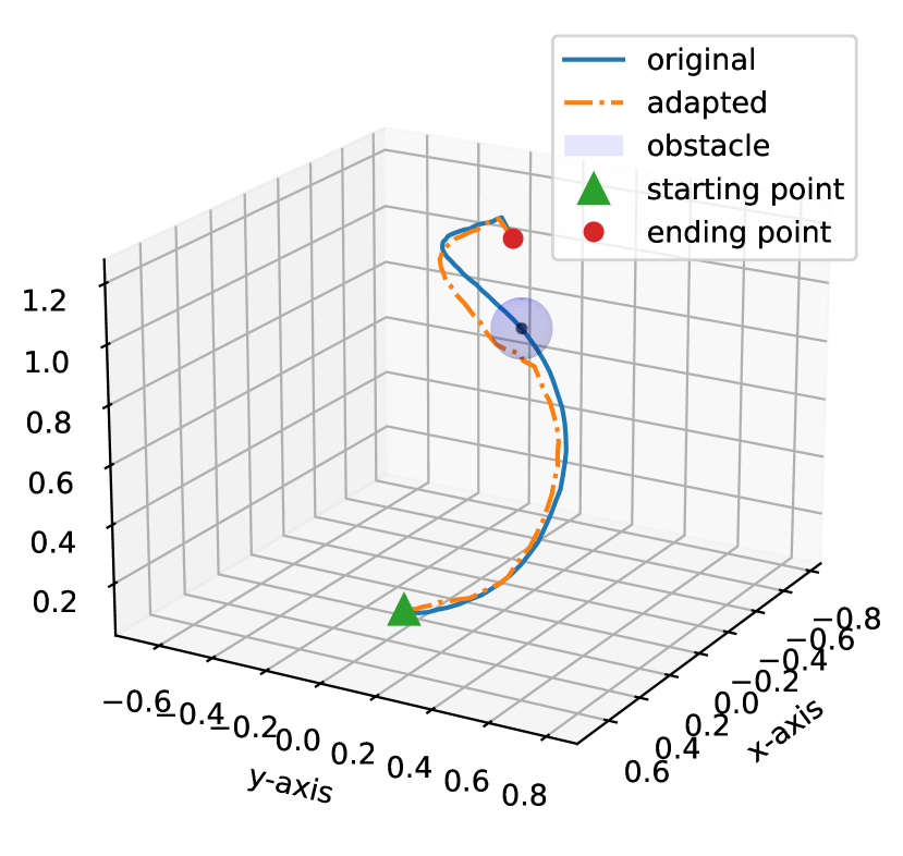
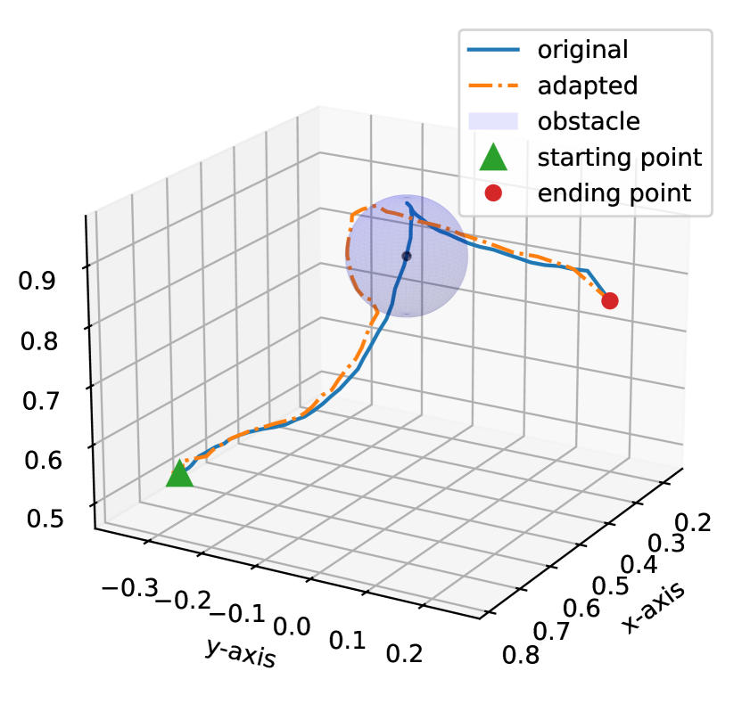
In the experiment, we used a beam search with a size of 25. The temperature of the output, which is the scale of the output STD, was set to two. Fig. 6 demonstrates how the adapted trajectories effectively navigate to avoid spherical obstacles for samples drawn from both the prior and posterior distributions.

IV-D3 Position bound

Figure 7: Motion adaptation for position boundary. Colors indicate the axes of the Cartesian coordinate.

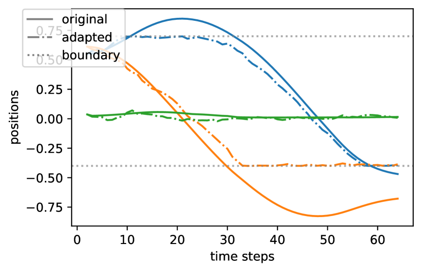
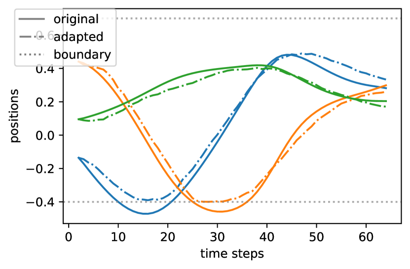
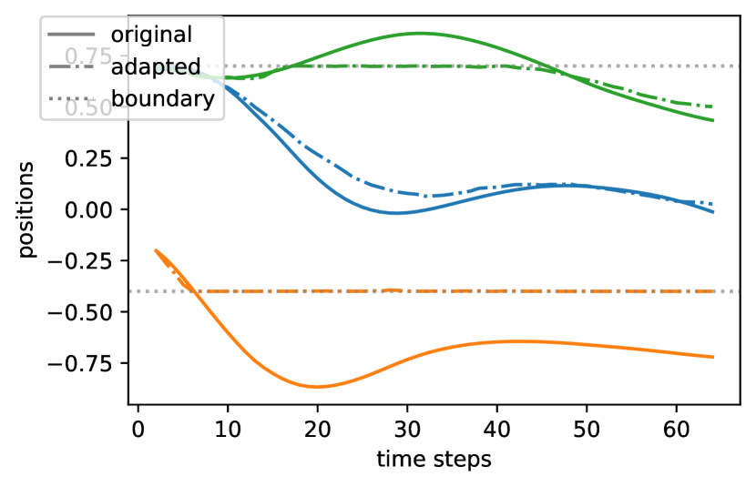
As depicted in Figure 7, the generated trajectories are supposed to follow the original demonstrations, with adaptations made to ensure compatibility within the cuboid boundaries.

IV-D4 Velocity and acceleration bound

Table I: Velocity and acceleration limits.

methods	samples	max values
velocity bound	prior	0.050
	posterior	0.050
	boundary	0.050
	original data	0.094
acceleration bound	prior	0.020
	posterior	0.020
	boundary	0.020
	original data	0.031

We have established boundaries for both velocity and acceleration, as detailed in Table LABEL:tab:v_a_limit. Although the table presents only a single boundary for each type of boundary, these boundaries can be set to arbitrary values.

V Conclusion

In this paper we introduce a novel Transformer-based auto-encoder framework for robot motion generation and adaptation, leveraging Learning from Demonstration (LfD). The latent space of the autoencoder can be viewed a motion representation similarly as in movement primitives. The conditioning of the trajectory generation on goal an motion representation is implemented through flexible cross-attention mechanisms. By using an autoregressive decoder and online (approximate) inference methods our approach generates trajectories that adapt to various task space constrains such as obstacle avoidance, via-points, and various position, velocity, and acceleration bounds. The experiments validated the framework’s robustness and adaptability across different robots and various trajectory constraints.

-A Training

Training VAEs and CVAEs can be challenging due to local minima, posterior collapse or over-regularization [20, 21, 22]. Sequence-to-sequence models with strong decoders are often prone to posterior collapse. The authors in [23] reduced the capability of the decoder using the hierarchical decoder. Alternatively, reformulating the objective or using specialized training strategies can also alleviate some optimization problems. The authors in [24] reformulate training as a constrained optimization problem where the reconstruction term $-\mathrm{E}_{\hat{p}(x_{1:T})}\mathrm{E}_{q_{\phi}(z;x_{1:T})}[\log p_{\theta}(x_{2:T-1}|x_{1,T},z)]$ term is constrained to achieve specific reconstruction accuracy. The authors in [25] train a hierarchical VAE model using a similar reformulation and use a scheduled pre-training of the reconstruction term. To attain a required reconstruction loss (powerful decoder) and to also avoid posterior collapse we formulate the optimization problem as

$$\min_{\theta,\phi} \>1$$

$$\mathrm{s.t.} \>\mathrm{E}_{\hat{p}(x_{1:T})}\mathrm{E}_{q_{\phi}(z;x_{1:T})}[-\log p_{\theta}(x_{2:T-1}|x_{1,T},z)]\leq\xi_{\mathrm{rec}}$$

$$\>\mathrm{E}_{\hat{p}(x_{1:T})}\mathrm{KL}[q_{\phi}(z;x_{1:T})\,\|\,p_{\theta}(z;x_{1,T})]\leq\xi_{\mathrm{kl}}.$$

The resulting Lagrangian will have two multipliers $\lambda_{\mathrm{rec}}$ and $\lambda_{\mathrm{kl}}$ that adaptively re-weight the reconstruction and the KL (regularization) terms. We use the exponential method of multipliers [26], that is, we apply the update $\lambda_{\mathrm{kl}}^{(k+1)}=\lambda_{\mathrm{kl}}^{(k)}\cdot\exp\{\eta(-\mathrm{E}_{\hat{p}(x_{1:T})}\mathrm{KL}[q_{\phi}(z;x_{1:T})\,\|\,p_{\theta}(z;x_{1,T})]+\xi_{\mathrm{kl}})\}$ and a corresponding one for $\lambda_{\mathrm{rec}}$.

-B Architecture and computation

The computational analyses of this research used an NVIDIA GeForce GTX 1080 Ti GPU, with PyTorch version 2.1.0 for implementation.

The model’s encoder depth was set to 3, with an embedding dimension of 16, and a latent vector length of 32. The decoder was configured with 8 heads and 10 layers. For optimization, the RAdam optimizer [27], was chosen, configured with beta values of 0.9 and 0.999, and a learning rate of 0.0005. Batch sizes were 256 for the data in Cartesian space and 128 for the joint space. Mixup [28] was used as a data augmentation for the joint space data.

References

- [1] S. Schaal, “Dynamic movement primitives-a framework for motor control in humans and humanoid robotics,” in Adaptive motion of animals and machines. Springer, 2006, pp. 261–280.
- [2] A. J. Ijspeert, J. Nakanishi, H. Hoffmann, P. Pastor, and S. Schaal, “Dynamical movement primitives: learning attractor models for motor behaviors,” Neural computation, vol. 25, no. 2, pp. 328–373, 2013.
- [3] A. Paraschos, C. Daniel, J. R. Peters, and G. Neumann, “Probabilistic movement primitives,” Advances in neural information processing systems, vol. 26, 2013.
- [4] N. D. Ratliff, J. Issac, D. Kappler, S. Birchfield, and D. Fox, “Riemannian motion policies,” arXiv preprint arXiv:1801.02854, 2018.
- [5] K. Sohn, H. Lee, and X. Yan, “Learning structured output representation using deep conditional generative models,” Advances in neural information processing systems, vol. 28, 2015.
- [6] A. Jaegle, F. Gimeno, A. Brock, O. Vinyals, A. Zisserman, and J. Carreira, “Perceiver: General perception with iterative attention,” in International conference on machine learning. PMLR, 2021, pp. 4651–4664.
- [7] A. Vaswani, N. Shazeer, N. Parmar, J. Uszkoreit, L. Jones, A. N. Gomez, Ł. Kaiser, and I. Polosukhin, “Attention is all you need,” Advances in neural information processing systems, vol. 30, 2017.
- [8] J. Devlin, M.-W. Chang, K. Lee, and K. Toutanova, “Bert: Pre-training of deep bidirectional transformers for language understanding,” arXiv preprint arXiv:1810.04805, 2018.
- [9] T. Wang and X. Wan, “T-cvae: Transformer-based conditioned variational autoencoder for story completion.” in IJCAI, 2019, pp. 5233–5239.
- [10] F. Frank, A. Paraschos, P. van der Smagt, and B. Cseke, “Constrained probabilistic movement primitives for robot trajectory adaptation,” IEEE Transactions on Robotics, vol. 38, no. 4, pp. 2276–2294, 2021.
- [11] P. Koehn, Statistical machine translation. Cambridge University Press, 2009.
- [12] M. Post and D. Vilar, “Fast lexically constrained decoding with dynamic beam allocation for neural machine translation,” arXiv preprint arXiv:1804.06609, 2018.
- [13] D.-H. Park, H. Hoffmann, P. Pastor, and S. Schaal, “Movement reproduction and obstacle avoidance with dynamic movement primitives and potential fields,” in Humanoids 2008-8th IEEE-RAS International Conference on Humanoid Robots. IEEE, 2008, pp. 91–98.
- [14] H. Hoffmann, P. Pastor, D.-H. Park, and S. Schaal, “Biologically-inspired dynamical systems for movement generation: Automatic real-time goal adaptation and obstacle avoidance,” in 2009 IEEE International Conference on Robotics and Automation, 2009, pp. 2587–2592.
- [15] N. Chen, J. Bayer, S. Urban, and P. Van Der Smagt, “Efficient movement representation by embedding dynamic movement primitives in deep autoencoders,” in 2015 IEEE-RAS 15th international conference on humanoid robots (Humanoids). IEEE, 2015, pp. 434–440.
- [16] N. Chen, M. Karl, and P. Van Der Smagt, “Dynamic movement primitives in latent space of time-dependent variational autoencoders,” in 2016 IEEE-RAS 16th international conference on humanoid robots (Humanoids). IEEE, 2016, pp. 629–636.
- [17] D. Koert, G. Maeda, R. Lioutikov, G. Neumann, and J. Peters, “Demonstration based trajectory optimization for generalizable robot motions,” in 2016 IEEE-RAS 16th International Conference on Humanoid Robots (Humanoids), 2016, pp. 515–522.
- [18] D. Koert, J. Pajarinen, A. Schotschneider, S. Trick, C. Rothkopf, and J. Peters, “Learning intention aware online adaptation of movement primitives,” IEEE Robotics and Automation Letters, vol. 4, no. 4, pp. 3719–3726, 2019.
- [19] A. Padalkar, A. Pooley, A. Jain, A. Bewley, A. Herzog, A. Irpan, A. Khazatsky, A. Rai, A. Singh, A. Brohan, et al., “Open x-embodiment: Robotic learning datasets and rt-x models,” arXiv preprint arXiv:2310.08864, 2023.
- [20] T. Sønderby, C. K.and Raiko, L. Maaløe, S. K. Sønderby, and O. Winther, “Ladder variational autoencoders,” NeurIPS, 2016.
- [21] S. R. Bowman, L. Vilnis, O. Vinyals, A. M. Dai, R. Jozefowicz, and S. Bengio, “Generating sentences from a continuous space,” arXiv preprint arXiv:1511.06349, 2015.
- [22] D. P. Kingma, T. Salimans, R. Jozefowicz, X. Chen, I. Sutskever, and M. Welling, “Improved variational inference with inverse autoregressive flow,” Advances in neural information processing systems, vol. 29, 2016.
- [23] A. Roberts, J. Engel, C. Raffel, C. Hawthorne, and D. Eck, “A hierarchical latent vector model for learning long-term structure in music,” in International conference on machine learning. PMLR, 2018, pp. 4364–4373.
- [24] D. J. Rezende and F. Viola, “Taming VAEs,” CoRR, 2018.
- [25] A. Klushyn, N. Chen, R. Kurle, B. Cseke, and P. van der Smagt, “Learning hierarchical priors in VAEs,” Advances in Neural Information processing Systems, vol. 32, 2019.
- [26] D. P. Bertsekas, Nonlinear Programming: Second Edition. Athena Scientific, 2003.
- [27] L. Liu, H. Jiang, P. He, W. Chen, X. Liu, J. Gao, and J. Han, “On the variance of the adaptive learning rate and beyond,” arXiv preprint arXiv:1908.03265, 2019.
- [28] H. Zhang, M. Cisse, Y. N. Dauphin, and D. Lopez-Paz, “mixup: Beyond empirical risk minimization,” arXiv preprint arXiv:1710.09412, 2017.