GCN-DevLSTM: Path Development for Skeleton-Based Action Recognition

Abstract

Skeleton-based action recognition (SAR) in videos is an important but challenging task in computer vision. The recent state-of-the-art models for SAR are primarily based on graph convolutional neural networks (GCNs), which are powerful in extracting the spatial information of skeleton data. However, it is yet clear that such GCN-based models can effectively capture the temporal dynamics of human action sequences. To this end, we propose the DevLSTM module, which exploits the path development – a principled and parsimonious representation for sequential data by leveraging the Lie group structure. The path development, originated from Rough path theory, can effectively capture the order of events in high-dimensional stream data with massive dimension reduction and consequently enhance the LSTM module substantially. Our proposed G-DevLSTM module can be conveniently plugged into the temporal graph, complementing existing advanced GCN-based models. Our empirical studies on the NTU60, NTU120 and Chalearn2013 datasets demonstrate that our proposed hybrid model significantly outperforms the current best-performing methods in SAR tasks. The code is available at https://github.com/DeepIntoStreams/GCN-DevLSTM.

1 Introduction

Action recognition has a wide range of applications in diverse fields such as human-computer interaction, performance assessment in athletics, virtual reality, and video monitoring Liu et al. (2019a). In comparison to video-based action recognition, skeleton-based action recognition (SAR) exhibits better robustness to the variety of light conditions and its efficiency in computation and storage Chen et al. (2021); Shi et al. (2019) while preserving data privacy. Skeleton data can be obtained either by localisation of 2D/3D human joints using the depth camera Liu et al. (2019a) or pose estimation algorithms from the videos Cao et al. (2017).

Despite extensive literature devoted to SAR, the challenge still remains open. The key step towards accurate SAR models lies in designing an effective spatio-temporal representation of the skeleton sequence. Previously, Recurrent Neural Network (RNN) was commonly used due to its strength in capturing the temporal dynamics. However, since STGCN Yan et al. (2018) was proposed to capture the spatio-temporal features, which contain spatial graph convolution and temporal convolution, graph convolutional networks (GCNs) have taken precedence. The majority of subsequent GCN-based approaches Chen et al. (2021); Shi et al. (2019, 2020); Cheng et al. (2020b, a); Song et al. (2020) have largely followed the STGCN framework, while they mainly focus on the improvement of the spatial graph convolution, with minimal emphasis on improving temporal modules. All of these methods rely on $K\times 1$ convolution operation to capture temporal features, where $K$ represents the kernel size of the convolutional operation in the temporal receptive field. However, whether convolution operation is most effective for capturing temporal dynamics is in question.

On the other hand, Rough path theory  Lyons (1998) originated as a branch of stochastic analysis to make sense of controlled differential equations driven by highly oscillatory paths. More recently, the applications of rough path theory in sequential data analysis are emerging. In particular, the path signature, as a fundamental object of Rough path theory, has successful applications in various domains ranging from finance to healthcare, demonstrating its capacity as a principled and efficient feature of time series. By embedding time series into the continuous path space, the signature offers a unified treatment to handle variable length and irregular sampling. Signature-based algorithms show promise across diverse fields, including SAR task Liao et al. (2021); Yang et al. (2022); Ahmad et al. (2019); Li et al. (2019a); Cheng et al. (2023). However, the path signature may face challenges such as the curse of dimensionality caused by high path dimension and lack of adaptability due to its deterministic nature Lou et al. (2022). To address these, Lou et al. Lou et al. (2022) propose the path development from rough path theory, as a trainable alternative to path signature. The path development enjoys the desirable properties of the signature while reducing feature dimension significantly.  Lou et al. (2022) shows that combining the path development under the appropriate Lie group with LSTM Hochreiter and Schmidhuber (1997) successfully alleviates the gradient vanishing issues of LSTMs, leading to significant enhancement across various sequential tasks.

This paper places a primary emphasis on enhancing the temporal module within our framework. While retaining the effectiveness of graph convolution for modelling spatial relationships among joints, we introduce a novel module, G-DevLSTM, for handling temporal relationships of the graph with the node feature as time series. More specifically, we adopt a topology-non-shared graph from CTRGCN Chen et al. (2021) where each channel has an adjacency matrix while in contrast to employing only convolutional operation in the temporal module, we also integrate path development and LSTM in our framework. This combination enables our temporal block to capture more discriminative temporal features, leading to model performance improvement. Experimental results on three commonly used datasets show that our approach outperforms other methods, demonstrating the effectiveness of our proposed temporal module.

We summarise our main contributions as follows:

• We design a novel and principled graph development (G-Dev) layer for analysing temporal graph data by extending the path development originally applied to vector-valued time series. As a generic network on graph data with time-varying node attributes, G-Dev exhibits efficacy and robustness to irregular sampling and missing data.

• We introduce the novel GCN-DevLSTM network for skeleton-based action recognition that effectively combines the G-Dev layer with LSTM to capture complex temporal dynamics.

• Experimental results demonstrate that our designed model outperforms other state-of-the-art models in SAR in terms of accuracy and robustness.

2 Related Work

2.1 Skeleton-based Action Recognition

SAR is a task where we need to consider both spatial and temporal relationships. Earlier methods normally use convolutional neural networks (CNNs) Chéron et al. (2015); Liu et al. (2017b) and RNN Du et al. (2015); Liu et al. (2017a) to address both spatial and temporal challenges without considering structural topology. STGCN Yan et al. (2018) is the first method to capture spatial and temporal relationships using GCN, taking the skeleton topology of the graph into consideration while this topology is not learnable, with only the spatial connection between adjacent joints being connected. As a result, some actions required to consider non-adjacent joints may perform poorly. Liu et al. (2020) addresses this by introducing a learnable adjacency matrix alongside the original manually defined one, enabling connections between non-neighboring joints. Yet, this approach maintains the same graph for all action inputs, which is not ideal, as different action classes may benefit from different graph topologies. To address this, Li et al. (2019b); Shi et al. (2019, 2020) propose adaptive graph convolutional network, allowing the topology to be learnable and data dependent while they still use the same topology for all channels. Cheng et al. (2020a); Chen et al. (2021) further propose non-shared topology which uses distinct topology for each channel. Current GCN-based methods put much effort into the enhancement of the graph, with limited attention to temporal design. Most GCN-based methods mainly rely on CNNs to capture temporal dynamics. Although studies such as Si et al. (2019); Zhao et al. (2019); Liao et al. (2021) utilise LSTM to capture temporal features while also using GCN to build spatial correlations, these models unfortunately experience a performance lag compared to those leveraging both GCN and CNN.

2.2 Path signature & Path Development

Path signature, introduced by Chen Chen (1958), is a representation of a piecewise regular path. This representation involves a collection of iterated integrals, which faithfully represent the original path. Lyons further broadens the scope from paths with bounded variation Hambly and Lyons (2010) to paths with finite p-variation for any $p\geq 1$ Boedihardjo et al. (2016). There are plenty of applications of path signature in various machine learning areas, containing handwritten recognition Xie et al. (2017), writer identification Yang et al. (2015), financial data analysis Lyons et al. (2014), time-series data generation Ni et al. (2021) and SAR Liao et al. (2021); Cheng et al. (2023); Yang et al. (2022); Ahmad et al. (2019); Li et al. (2019a). In the specific context of SAR, Ahmad et al. (2019) focuses on employing path signature solely for extracting spatial features while Yang et al. (2022); Li et al. (2019a) utilise path signature to obtain both temporal-spatial features. However, relying solely on path signature to capture spatial relationships may be suboptimal as it is not data adaptive and only considers local spatial correlations. Recognising the efficacy of GCN in modelling spatial relationships, Liao et al. (2021) leverages GCN to extract spatial features and employ path signature to capture temporal dynamics. Unfortunately, the network tends to overfit rapidly when increasing its depth due to the excessively large output dimension of the signature.

Trainable path development, as presented in the work Lou et al. (2022) is based on the development of a path à la Cartan Driver (1995), a significant mathematical tool in rough path theory, particularly for the examination of the inverse of the signature Lyons and Xu (2017) and the uniqueness of expected signature Hambly and Lyons (2010); Chevyrev and Lyons (2016). Chevyrev and Lyons (2016) demonstrates that given an appropriate Lie algebra, the path development has universal and characteristic properties, just like path signature, suggesting the potential of path development as a promising feature representation for sequential data. Moreover, path development has been successfully applied in PCF-GAN Lou et al. (2023) to generate high-quality time series data due to the favourable non-commutativity and group structure of the unitary feature.

This paper is built upon the path development. Instead of solely relying on CNN to capture temporal dynamics, we integrate path development with LSTM and propose a new temporal module to capture more discriminate temporal features.

3 G-Dev Layer: Development layer of a temporal graph

In this section, we start with a concise overview of the development of the path as the principled feature representation of $d$-dimensional time series. Subsequently, we proceed with introducing the path development layer proposed in Lou et al. (2022). For details of the path development, we refer readers to Lou et al. (2022). Building on this, we propose the G-Dev layer, a novel extension of the development layer applied to temporal graphs, wherein the features of nodes are represented by time series.

3.1 The development of a Path

Let $X\in V([0,T],\mathbb{R}^{d})$, where $V([0,T],\mathbb{R}^{d})$ represents the space of continuous paths of finite length in $\mathbb{R}^{d}$ defined on the time interval $[0,T]$. To fix the notations, let $G$ denote a finite-dimensional Lie group and its associate Lie algebra $\mathfrak{g}$. Examples of the matrix Lie algebra associated with the special orthogonal group (denoted by $\mathfrak{so}$) and special Euclidean group ($\mathfrak{se}$) are given as follows:

$$\mathfrak{gl}(m;\mathbb{F})=\{m\times m\text{ matrices over }\mathbb{F}\}\cong\mathbb{F}^{m\times m}\quad(\mathbb{F}=\mathbb{R}\text{ or }\mathbb{C})$$

$$\mathfrak{so}(m,\mathbb{R}):=\{A\in\mathfrak{gl}(m;\mathbb{R}):A^{T}+A=0\}$$

$$\mathfrak{se}(m)=\left\{\begin{bmatrix}\omega&v\\ 0&0\end{bmatrix}\mid\omega\in\mathfrak{so}(m,\mathbb{R}),\ v\in\mathbb{R}^{m}\right\}$$

Definition 3.1 (Path Development).

Let $M:\mathbb{R}^{d}\rightarrow\mathfrak{g}\subset\mathfrak{gl}(m)$ be a linear map. The path development of $X\in V([0,T],\mathbb{R}^{d})$ on $G$ under $M$ is the solution $Z_{T}\in G$ to the below equation

$$dZ_{t}=Z_{t}\cdot M(dX_{t})\quad\text{for all }t\in[0,T]\quad\text{with }Z_{0}=\text{Id}_{m},$$ (1)

where $\text{Id}_{m}$ is the identity matrix and $\cdot$ denotes the matrix multiplication.

Example 1 (Linear path).

Let $X\in V([0,T],\mathbb{R}^{d})$ be a linear path. For any linear map $M\in L(\mathbb{R}^{d},\mathfrak{g})$, the development of the path under $M$ admits the explicit formula and is simply

$$D_{M}(X)_{0,T}=\exp\left(M(X_{T}-X_{0})\right),$$ (2)

where $\exp$ is the matrix exponential.

Thanks to the multiplicative property of the path development (Lemma 2.4 in Lou et al. (2022)), the development of two paths $X\in V([0,s],\mathbb{R}^{d})$ and $Y\in V([s,t],\mathbb{R}^{d})$ under $M$ is the same as the development of the concatenation of these two path, in formula,

$$D_{M}(X*Y)=D_{M}(X)\cdot D_{M}(Y),$$ (3)

where $X*Y$ denotes the concatenation of $X$ and $Y$ and $\cdot$ is the matrix multiplication. Eq. (3) enables us to compute the development of any piecewise linear path explicitly.

The path development enjoys several desirable theoretical properties, which makes itself a principled and efficient representation of sequential data. We summarise the properties, which are directly relevant to action recognition as follows.

Invariance under Time-reparametrisation

Similar to the path signature, the path development is invariant under time reparametrisation. This property ensures that the development of a path remains unchanged irrespective of the speed at which the path is traversed. It is well suited to action recognition, as the prediction of actions should not depend on the speed of the actions or the frame rate. Time-reparametrisation invariance of path development may bring massive dimension reduction and enhance the robustness to variation in speed.

Uniqueness of the path development

Intuitively, the path development effectively capture the order of events in time series, leveraging the non-commutative nature of matrix multiplication. Changing the order of events may lead to different development in general, highlighting its capacity to capture the temporal dynamics of sequential data. It is proven in Chevyrev and Lyons (2016) the path development is a characteristic and universal feature of an un-parameterised path in $V_{1}([0,T],\mathbb{R}^{d})$ under the appropriate Lie group. In other words, transforming a path of finite length to its development map $M\mapsto\text{Dev}_{M}(X)$ can uniquely determine the path $X$ and yield no information loss.

3.2 Path Development Layer

Proposed in  Lou et al. (2022), the path development layer is a novel neural network inspired by the path development by exploiting the representation of the matrix Lie group. More specifically, this layer utilises the parameterised linear map $M\in L(\mathbb{R}^{d},\mathfrak{g})$ by its linear coefficients $\theta\in\mathfrak{g}^{d}$.

Definition 3.2 (Path development layer).

The path development layer, denoted by $D_{\theta}$, is defined as a mapping $\mathbb{R}^{d\times(N+1)}\rightarrow G$, which transforms any input time series $x=(x_{1},x_{2},...,x_{N})$ to the development $z_{N}\in G$ under the trainable linear map $M_{\theta}\in L(\mathbb{R}^{d},\mathfrak{g})$. Here for $n\in\{0,...,N-1\}$, we set

$$z_{n+1}=z_{n}\exp(M_{\theta}(x_{n+1}-x_{n})),z_{0}=Id_{m},$$ (4)

where $\theta\in\mathfrak{g}^{d}$ is the model parameter.

Eq. (4) is a direct consequence of Example 1 and the multiplicative property of the development (Eq. (3)). Moreover, Eq. (4) shows the recurrence as an analogy to that of the RNNs, albeit in a much simpler manner, as depicted in Figure 1 (lower panel). Similar to RNNs, the path development can cope with time series input of variable length.

Dimension reduction

The output of the path development has dimension $m^{2}$, where $m$ is the matrix size. Note that its dimension does not depend on the path dimension $d$ and time dimension $T$, resulting in the massive dimension reduction. This is in stark contrast to the signature feature of degree $k$, whose dimension $\left(\sum_{i=0}^{k}{d^{i}}=\frac{d^{k+1}-1}{d-1}\right)$ grows geometrically w.r.t $d$. Moreover, the path development is well suited to extract information from high-frequency time series or long time series without concern on the curse of dimensionality.

Robustness to irregular sampling

As the path development can be interpreted as a solution to the differential equation (Eq. (1), it is a continuous time series model. Similar to other continuous time models such as signature and Neural CDEs Kidger et al. (2020), the path development exhibits robustness in handling time series data with irregular sampling.

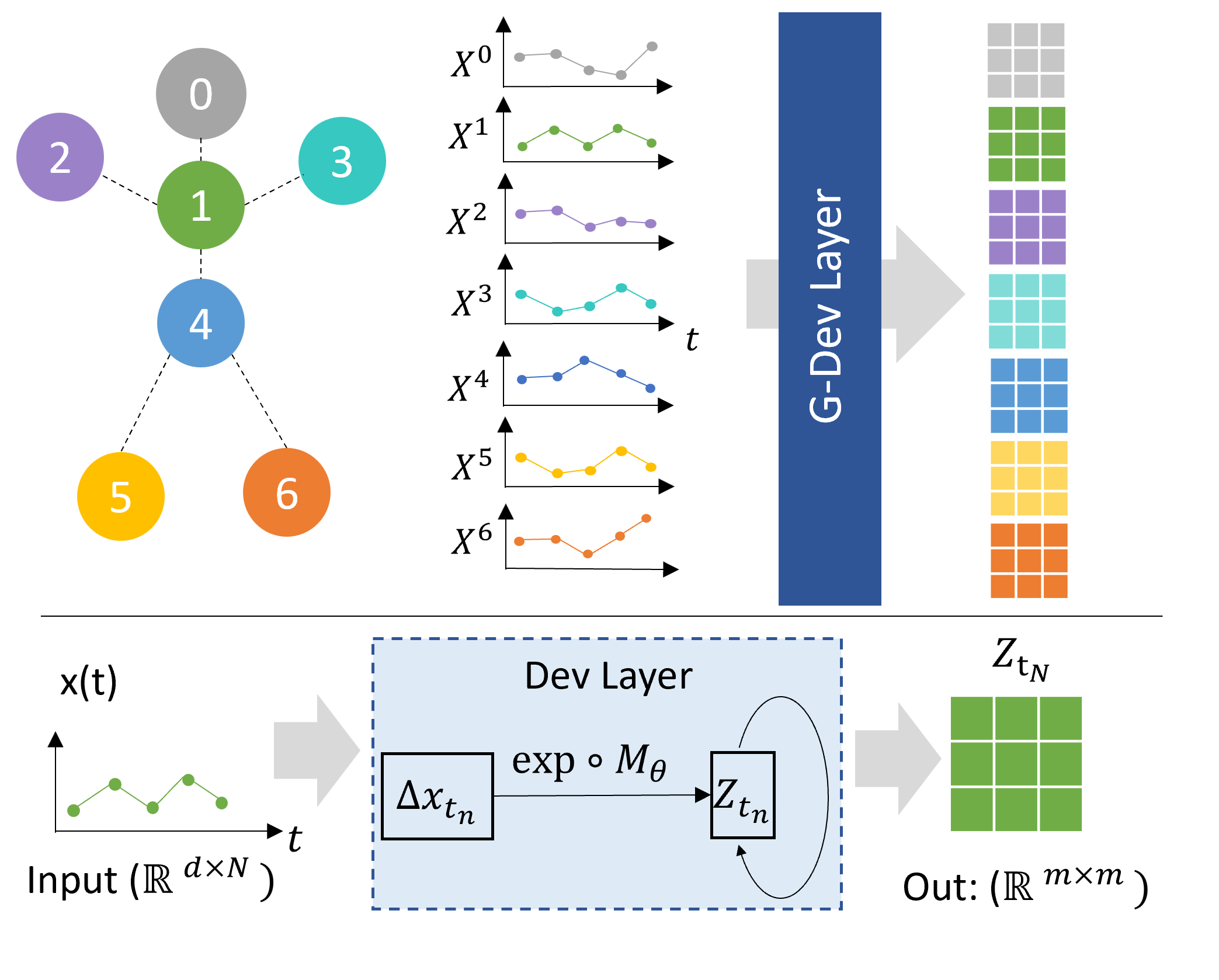
Figure 1: The work flow of G-Dev layer.

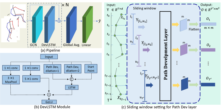
Figure 2: (a) The pipeline of our proposed approach consists of $N$ blocks, with each block containing a GCN module and a DevLSTM module. (b) The detail of the DevLSTM module of (a) is provided here. (c) The flowchart illustrates the sliding window setting for the path development layer in (b).

3.3 G-Dev Layer: Apply path development layer to a temporal graph

In this subsection, we propose the so-called G-Dev Layer, which serves as a generalisation of the development layer from the $d$-dimensional time series to the temporal graph. Throughout this paper, the temporal graph $\mathfrak{G}=(\mathcal{V},\mathcal{E},X)$ refers to the graph with each node associated with $d$-dimensional time series features. Here $\mathcal{V}:=\{v^{1},\cdots,v^{M}\}$ denotes the vertex set and $\mathcal{E}$ can be represented by the adjacent matrix $A\in\mathbb{R}^{m\times m}$. Let $X^{i}=(x_{t_{1}},\cdots,x_{t_{N_{i}}})\in\mathbb{R}^{d\times N_{i}}$ denote the features of the $i^{th}$ vertex, where $d$ and $N_{i}$ are the path and time dimension, respectively. The time dimension $N_{i}$ may vary across vertices $v_{i}$ for $i\in\{1,\cdots,M\}$. The feature sets $X=(X^{(1)},\cdots,X^{(M)})$ is obtained by stacking $X^{i}$ for all $i\in\{1,\cdots,M\}$. Clearly, the skeleton sequence is an example of temporal graph data.

The proposed G-Dev Layer is the transformation of the temporal graph by applying the development layer to the time-augmented transformation of each feature vector $X_{i}$ of the vertex $v_{i}$. The G-Dev layer is a trainable layer with model parameters $\theta\in\mathfrak{g}^{d}\subset\mathbb{R}^{m\times m\times d}$. As shown in Figure  1, at each vertex $V_{i}$, we apply the development transformation to its associated time series feature $X^{(i)}$, resulting in the matrix-valued output $Z_{t_{N}}\in G\subset\mathbb{R}^{m\times m}$.

4 GCN-DevLSTM Network for SAR

A skeleton sequence can be modelled by a temporal graph, where the vertex set corresponds to $M$ possible joints, with each $v^{i}\in\mathbb{R}^{2}$ or $\mathbb{R}^{3}$ indicating 2 or 3$D$ coordinates of the $i^{\text{th}}$ joint, respectively. The edge set $\mathcal{E}$ denotes the set of all the joint pairs connected by a bone. The feature of each vertex $V^{i}:=(V_{1}^{i},\cdots,V_{T}^{i})$ represents the trajectory of $i^{\text{th}}$ joint with $V_{t}^{(i)}$ being its location at time $t$.

We illustrate the pipeline of our method in Figure 2(a). As shown in Figure 2(a), we treat the GCN and the DevLSTM module as an integrated block. GCN module focuses on capturing spatial correlations among vertices, while DevLSTM module is designed to capture temporal dynamics of the temporal graph across video frames. Detailed explanations of the GCN and DevLSTM modules will be provided in the subsequent sections. Our network is designed to capture discriminative spatial-temporal features with $N$ such blocks, where $N$ is set to 9 in this paper. Additionally, within each block, we build a residual path that establishes a shortcut connection with the input, which can mitigate issues related to gradient vanishing and explosion, enhancing the training stability of the model.

Following these GCN-DevLSTM blocks, we employ global average pooling to effectively reduce both temporal and spatial dimensions to 1. After that, a linear function is applied to adjust the feature dimension to match the number of action classes, thereby facilitating the classification process. Cross-entropy loss is employed at the end to compare the predicted action class with the ground truth.

4.1 GCN Module

In the GCN module, we basically follow the structure of CTR-GC Chen et al. (2021). However, we depart from the use of three initial adjacency matrices representing self, inward, and outward correlations. Instead, we enhance the model by incorporating various hops of information to construct three adjacency matrices denoted as $A_{0}$, $A_{1}$, and $A_{2}$.

$A_{0}$ remains an identical (self) matrix. For $A_{1}$, the elements $a_{ij}$ are set to 1 if vertex i and vertex j are physically connected in the skeleton graph; otherwise $a_{ij}$ in $A_{1}$ is set to 0. $A_{1}$ captures the direct connections in the graph. To enrich spatial information, we introduce $A_{2}=A_{1}^{2}$, enabling a vertex to connect with its neighbour’s neighbour. $A_{2}$ allows us to extend our understanding beyond direct connections to include relationships involving two hops in the graph.

Following CTR-GC, we utilise a network to dynamically learn an adjacency matrix for each channel, adding it with $A_{k}$ for $k\in\{0,1,2\}$. This process can be expressed as:

$$A_{k}^{{}^{\prime}}(X)=A_{k}+\mathcal{F_{\theta}}(X)$$ (5)

where $A_{k}^{{}^{\prime}}$ represents the updated adjacency matrix, $A_{k}$ is the initial adjacency matrix for the $k$-th hop, and $\mathcal{F_{\theta}}(X)\in\mathbb{R}^{M\times M\times C}$ dynamically captures the spatial correlations of joints from the network, conditioned on the input data $X\in\mathbb{R}^{T\times M\times d}$, considering each channel of the output channels $C$. An overview of the CTR-GC is given in supplementary while details about the network of $\mathcal{F_{\theta}}(X)$ can be found in Chen et al. (2021).

After obtaining the input-conditioned adjacency matrix, the graph convolution is further performed as

$$Z_{t,c}=A_{k}^{{}^{\prime}}(X)_{c}\cdot(X_{t}\cdot W_{s})_{c}$$ (6)

where $Z\in\mathbb{R}^{T\times M\times C}$ is the output of GCN with the feature dimension $C$, and $W_{s}\in\mathbb{R}^{d\times C}$ denotes a feature transformation filter. We sum the outputs from three CTR-GC modules, each employing a distinct adjacency matrix. Subsequently, we apply batch normalisation and ReLU activation function to the summation result before sending it to the DevLSTM module.

4.2 DevLSTM Module

The core of our DevLSTM module is path development layer, where we employ a sliding-window-based strategy for processing time sequence data. Specifically, for each joint $V^{i}$, given time sequence data $Y\in\mathbb{R}^{T\times d}$, window (kernel) size $K$, dilation $D$, padding size $P$ and stride $S$, for $0\leq i\leq\frac{T-K-(K-1)(D-1)+2P}{S}-1$, we define each partition $Z_{i,D}\in Z$ as:

$$Z_{i,D}=[Y_{i\times S+p},Y_{i\times S+p+D},\dots,Y_{i\times S+p+(K-1)\cdot D}]$$ (7)

where $p$ is the offset to account for padding. To guarantee that we will not lose any information related to changes in the path, it is crucial to ensure a minimum one-point overlap between two consecutive time partitions.

We give an example in Figure 2(c) to clearly illustrate how we partition the given time sequence and process these partitions with path development layer. In the given example, the time sequence data $Y$ from a joint across time is segmented in a sliding-window way with the setting $K=4$, $D=1$, $S=2$, and at least one-point overlap is guaranteed. One shared path development layer then maps these partitions to the Lie group using Eq. 4 in a recurrent fashion. For each partition, we only retain the path development layer’s state at the final time point, ignoring the intermediate stages and the state will be further flattened from $m\times m$ to $1\times m^{2}$. We concatenate all flattened states from these partitions along the temporal dimension, thereby producing a new time sequence with the dimension $\mathbb{R}^{T{{}^{\prime}}\times m^{2}}$.

Inspired by the design of multi-scale tcn Liu et al. (2020), we also design a multi-scale network to capture temporal dynamics. We utilise $D=1$ and $D=2$ respectively to enable the path development layer to capture features at different time scales, enhancing the module’s ability to discern temporal patterns across different scales in the input sequence. Additionally, it’s worth noting that zero padding, a commonly employed technique in CNNs, may not be the most suitable choice for the path development layer from experimental results. In our approach, we opt for replicate padding.

Due to the translation invariance of the path development, we append the location of the starting points ($SP=Z_{D,0}$) to the output of the path development layer along the feature dimension over each sub-time interval. In formula, it can be expressed as

$$C_{i}=Concat(Dev_{\theta_{1}}(Z_{i,D=1}),Dev_{\theta_{2}}(Z_{i,D=2}),SP_{i})$$ (8)

where $C_{i}$ is the concatenation result at partition $i$, $Dev_{\theta_{1}}$ and $Dev_{\theta_{2}}$ are two distinct path development layers regarding to $D=1$ and $D=2$, respectively, and $SP_{i}$ is the first element of partition $i$. This step is crucial for uniquely determining a path, enhancing the effectiveness of the path development layer in capturing relevant temporal features.

Table 1: Experimental results on NTU-60 and NTU-120 dataset. The best results for each benchmark are bolded.

	Venue	NTU-60		NTU-120
		X-sub (%)	X-view (%)	X-sub (%)	X-view (%)
ST-GCN Yan et al. (2018)	AAAI’18	81.5	88.3	70.7	73.2
AGC-LSTM Si et al. (2019)	ICCV’19	89.2	95.0	-	-
Bayesian-LSTM Zhao et al. (2019)	ICCV’19	81.8	89.0	-	-
2S-AGCN  Shi et al. (2019)	CVPR’19	88.5	95.1	82.5	84.2
MS-AAGCN  Shi et al. (2020)	TIP’20	90.0	96.2	-	-
Shift-GCN  Cheng et al. (2020b)	CVPR’20	90.7	96.5	85.9	87.6
Logsig-RNN Liao et al. (2021)	BMVC’21	-	-	75.8	78.0
CTR-GCN(J) Chen et al. (2021)	ICCV’21	89.8	94.8	84.9	86.7
CTR-GCN(J+B) Chen et al. (2021)	ICCV’21	92.0	96.3	88.7	90.1
CTR-GCN Chen et al. (2021)	ICCV’21	92.4	96.8	88.9	90.6
EfficientGCN Song et al. (2022)	TPAMI’22	92.1	96.1	88.7	88.9
Ta-CNN Xu et al. (2022)	AAAI’22	90.4	94.8	85.4	86.8
FR-Head Zhou et al. (2023)	CVPR’23	92.8	96.8	89.5	90.9
Our method(J)		90.8	95.7	86.2	87.7
Our method(B)		91.1	95.2	87.0	88.6
Our method(D)		91.2	95.3	87.1	88.7
Our method(J+B)		92.4	96.4	89.0	90.4
Our method(J+B+JM+BM)		92.6	96.6	89.3	90.7
Our method(J+B+D+JM+BM)		92.9	96.6	89.7	91.2

The concatenated results $C=\{C_{0},C_{1},...,C_{N}\}$ where $N=\frac{T-K-(K-1)(D-1)+2P}{S}-1$, from two path development layers, along with their corresponding starting points, are subsequently fed into an LSTM network whose unit is crafted to selectively learn and store information over long sequences, enabling it to grasp long-term dependencies in data. There won’t be any changes to the temporal dimension before and after LSTM because all of LSTM’s hidden states at each time step will be utilised.

MaxPool and a convolutional layer with $5\times 1$ kernel size have consistently demonstrated superior performance within the temporal module of other GCN-based studies. Introducing both MaxPool and the $5\times 1$ convolutional operation to our DevLSTM temporal module has the potential to enhance model performance even further. We can reasonably design kernel size, padding, stride and dilation to ensure the output size of Maxpool, LSTM and $5\times 1$ convolution remain the same. As a result, we can sum up their outcomes to achieve improved overall performance.

5 Numerical Experiments

To validate the effectiveness of the proposed GCN-DevLSTM network, we carry out numerical experiments on the following popular benchmarking datasets for skeleton-based action and gesture recognition. (1) NTU RGB+D 60 (NTU-60) Shahroudy et al. (2016) consists of 56,880 action samples and 60 action classes, filmed by 40 people using three Kinect cameras in different camera views. 3D skeletal data in the dataset have different sequence lengths, with each owning 25 joints. (2) NTU RGB+D 120 (NTU-120) Liu et al. (2019b) extends upon NTU RGB+D 60, consisting of 114,480 samples and 120 action classes, filmed by 106 people in three camera views. We consider the Cross-subject (X-Sub) and Cross-view (X-View) evaluation benchmarks for both datasets as proposed by Shahroudy et al. (2016). (3) Chalearn2013 Escalera et al. (2013) is a public dataset for gesture recognition, consisting of 11,116 skeleton examples and 20 gesture categories, filmed by 27 people. We use only skeleton data from these datasets for our experiments.

Experiments are conducted using a single Nvidia A6000 graphics card, where a batch of 16 examples is fed to the network. Stochastic gradient descent optimiser Bottou (2012) is employed, with a Nesterov $\text{momentum}=0.9$ and a weight decay $=0.0003$. The training epoch is set to 65 and we apply the warm-up strategy He et al. (2016) to the first 5 epochs. The initial learning rate is 0.02 and a step learning rate decay is applied with a factor of 0.1 at epoch 35 and 55, respectively. Data processing on NTU datasets mainly follows the procedure in Chen et al. (2021), with the length of all input data sequences resizing to 64. We use $\mathfrak{se}$ Lie algebra in this paper, with a corresponding matrix size of $m=10$. A detailed network architecture can be found in the supplementary.

5.1 Dual graph

Since 2S-AGCN Shi et al. (2019) has demonstrated the effectiveness of combining predicted scores from different input data streams/representations, most of the recent approaches that we are set to compare adopt this technique for enhanced performance. The most commonly used data streams are joint (J), bone (B), joint motion (JM) and bone motion (BM) where details can be found in Shi et al. (2019, 2020). Apart from the above-mentioned data streams, we introduce a novel stream: the dual graph (D). In a dual graph, vertices represent bones, and edges establish connections between these bones. More details about dual graph can be checked at Supplementary Material. It’s clear from Table 1 that incorporating dual graph into the whole model, the overall accuracy can get further improved, especially on NTU-120 dataset, with 0.4$\%$ and 0.5$\%$ improvement on X-sub and X-view benchmarks respectively, stressing the importance of the introduced dual graph.

5.2 Comparison with state-of-the-art methods

We compare our approach with other state-of-the-art methods on both NTU-60 and NTU-120 datasets, as shown in Table 1. Since our GCN module is following CTR-GCN Chen et al. (2021) with the major difference lying in the temporal module, we show more results on CTR-GCN for a more comprehensive comparison. As we can see all of our results, no matter whether using only joint or using ensembled streams combining joint and bone, outperform CTR-GCN with a large margin on all benchmarks. Our method’s limited performance gain with extra joint or bone motion, compared to CTR-GCN, may stem from our path development layer exploiting position differences between consecutive time points. As a result, streams using joint and bone motion provide identical information at the beginning of the network, limiting their help. Our model, which integrates five data streams, achieves the best result compared to other state-of-the-art approaches across three benchmarks, with the exception of a close performance on the NTU60-Xview benchmark.

Table 2 shows the comparison results between our result and other state-of-the-art methods on Chalearn2013 dataset. We only employ the joint stream for fair comparison as other approaches only use the joint representation on Chalearn2013 dataset. It is evident that our method yields the best result again on the gesture dataset, further proving its superiority.

Table 2: Experimental results on Chalearn2013 dataset.

	Acc (%)
ST-LSTM + Trust Gate Liu et al. (2018)	92.00
Multi-path CNN Liao et al. (2019)	93.13
3s_net_TTM Li et al. (2019a)	92.08
GCN-Logsig-RNN Liao et al. (2021)	92.86
CTR-GCN Chen et al. (2021)	95.19
ST-PSM+L-PSM Cheng et al. (2023)	94.18
Our method	95.61

5.3 Comparison with signature-based models

Compared to the Logsig-RNN Liao et al. (2021), one of the recent signature-based action recognition methods (using the joint stream only), our model (J) outperforms 10.4% and 9.7% respectively on both benchmarks of NTU-120 dataset, and 2.75% on Chalearn2013 dataset. Compared to the latest signature-based action recognition approach Cheng et al. (2023), we still outperform 1.43% on Chalearn2013 dataset while unfortunately, they didn’t report their results on NTU dataset, leaving no way to compare. These results support the advantages of using path development that we claimed before, compared with path signature.

5.4 Comparison with MS-TCN

To demonstrate the flexible integration of our DevLSTM temporal module with various GCN modules in a plug-and-play fashion, we employ the adaptive graph convolution (AGC) graph in 2S-AGCN Shi et al. (2019) and a fixed graph without learnable parameters, respectively as an additional GCN module backbone in our network. In addition, we compare our DevLSTM with multi-scale temporal convolution network (MS-TCN) used in Chen et al. (2021) across the different GCN backbones. Table 3 illustrates that the proposed DevLSTM module consistently outperforms MS-TCN with different GCN backbones by a large margin, indicating that our designed temporal module is effective in enhancing various GCN backbones. An overview of adaptive graph convolution and fixed graph can be found in the supplementary material.

Table 3: Comparison between our DevLSTM module with MS-TCN across various GCN modules on NTU60 dataset.

GCN Module	Temporal module	X-sub	X-view
CTR-GC	MS-TCN (J)	90.3	94.9
	DevLSTM (J)	90.8	95.7
AGC	MS-TCN (J)	89.8	94.5
	DevLSTM (J)	90.6	95.6
Fixed graph	MS-TCN (J)	88.7	93.1
	DevLSTM (J)	89.5	94.5

5.5 Ablation studies

We further investigate the importance of each component in our temporal module. As evident from Table 4, the path development layer emerges as the primary contributor to the overall performance improvement since removing it causes the largest performance degradation, with other components also contributing to enhanced performance.

Table 4: Ablation studies of DevLSTM module on NTU-60 dataset.

Components	X-sub	X-view
with all components (J)	90.8	95.7
w/o 1$\times$ 1 conv & 5$\times$1 conv (J)	90.7	95.3
w/o 1$\times$ 1 conv & 3$\times$ 1 maxpool (J)	90.6	95.4
w/o path dev (J)	90.5	95.2

5.6 Robustness Analysis

We compare the robustness of our full model (GCN-DevLSTM), CTRGCN Chen et al. (2021) and our model without path development layer (GCN-LSTM) when missing frames happen. To this end, we create a new test dataset by randomly dropping a certain number of frames out of 64 frames and validate the model performance on this test dataset. Figure 3 illustrates that our full model with the path development layer consistently outperforms the other methods in terms of accuracy, regardless of the proportion of frames missing, proving its robustness to irregular sampling. More results are available in the supplementary material.

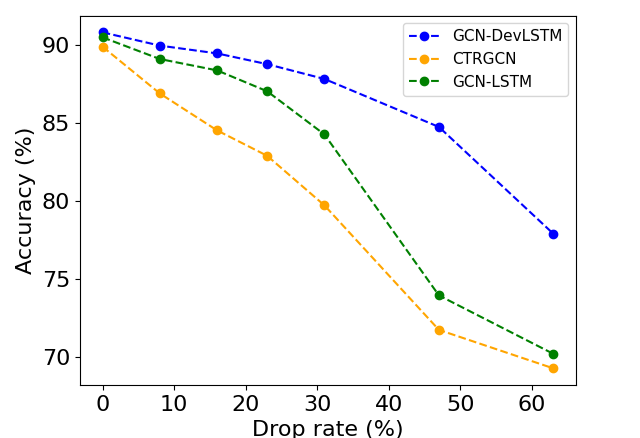
Figure 3: Robustness analysis against the dropping frames on NTU60-Xsub benchmark.

6 Conclusion

In summary, we propose a novel and general GCN-DevLSTM network for analysing temporal graph data by leveraging the path development layer. This approach not only offers flexibility when combined with various GCN modules but also significantly enhances performance by effectively capturing the temporal dependencies within data. The effectiveness of the proposed method is validated by the state-of-the-art results on both small gesture data and large action datasets in SAR. Moreover, it demonstrates superior robustness to missing data and variable frame rates.

Acknowledgements. LJ, WY and HN are supported by the EPSRC [grant number EP/S026347/1]. WY and HL are also supported by The Alan Turing Institute under the EPSRC grant EP/N510129/1.

7 Supplementary

7.1 Dual Graph Stream

Previous approaches Shi et al. [2019, 2020]; Chen et al. [2021]; Zhou et al. [2023] have commonly adopted a multi-stream architecture, including joint, bone, joint motion and bone motion, with each contributing to improved performance. Inspired by Li et al. [2019b] that leverages a dual graph as the model input, we also integrate a dual graph to enhance the performance of our model further. The definition of the dual graph is outlined below.

Given a pair of connected joints $V_{i}$ and joint $V_{j}$ in original skeleton graph representation, their bone $B_{ij}$ can be defined as follows:

$$B_{ij}=V_{i}-V_{j}$$ (9)

In the dual graph, these bones from the original skeleton graph serve as the joints, as depicted in Figure 4. Notably, the joint $V_{i-j}$ in the dual graph corresponds to the bone $B_{ij}$ in the original graph, and the edges connecting these joints of the dual graph represent bones. Specifically, when two joints in the dual graph share common elements, such as a pair of joints $V_{i-j}$ and $V_{k-j}$ both having the element $j$, an edge is established to connect these joints. This utilisation of a dual graph introduces a novel perspective, enhancing the overall performance of our model.

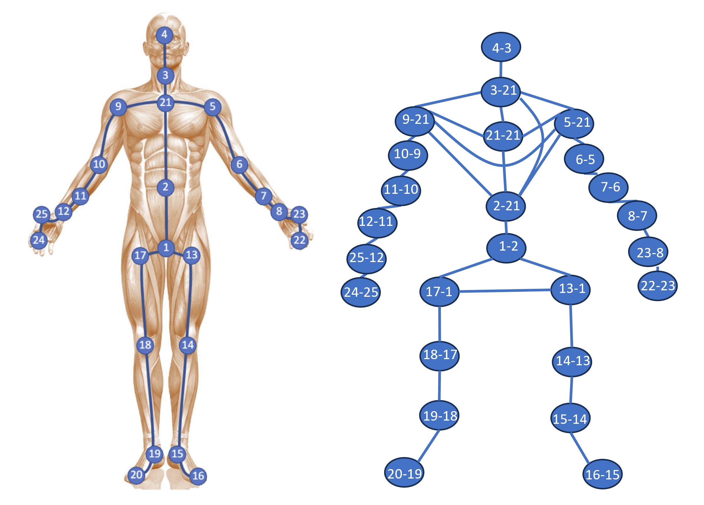
Figure 4: Dual Graph. Left side is the original skeleton representation in NTU dataset. The right side is its dual graph representation. Joint $V_{1-2}$ in the dual graph is the bone $B_{12}$ connecting joint $V_{1}$ and $V_{2}$ in original graph.

7.2 Detailed Network Architecture

Table 5 gives a detailed network architecture of our proposed approach. The entire network includes 9 blocks, in addition to a global average pooling layer and a linear layer. In the table, we report the output size of each block, including GCN and DevLSTM modules, as well as the output size of global average pooling layer and linear layer. In our configuration, $M$ is set to 2 on NTU dataset and 1 on Chalearn2013 dataset, representing the number of people in a video. $N$ is 19 on Chalearn2013 dataset and 25 on NTU-60 and NTU-120 datasets, representing the joint number. $T$ denotes the frame number. $T$ is 19 on Chalearn2013 dataset while on NTU60 and NTU120 datasets, we resize all videos with variable lengths to 64 frames. For the base channel size $C$, we set it as 64. Notably, the temporal dimension is reduced by half at blocks 5 and 8, respectively, by setting the $\text{stride}=2$ at the DevLSTM module. Last but not least, $N_{c}$ denotes the number of action classes, which is 120 on NTU-120 dataset and 20 on Chalearn2013 dataset, respectively.

Table 5: Detailed network architecture. $M$ denotes the number of people, $T$ denotes the frame number, $N$ denotes the number of joints, $C$ denotes the feature dimension and $N_{c}$ denotes the number of classes.

Blocks	Module Type	Output size
Block 1	GCN	$M\times T\times N\times C$
	DevLSTM	$M\times T\times N\times C$
Block 2	GCN	$M\times T\times N\times C$
	DevLSTM	$M\times T\times N\times C$
Block 3	GCN	$M\times T\times N\times C$
	DevLSTM	$M\times T\times N\times C$
Block 4	GCN	$M\times T\times N\times C$
	DevLSTM	$M\times T\times N\times C$
Block 5	GCN	$M\times T\times N\times 2C$
	DevLSTM	$M\times T/2\times N\times 2C$
Block 6	GCN	$M\times T/2\times N\times 2C$
	DevLSTM	$M\times T/2\times N\times 2C$
Block 7	GCN	$M\times T/2\times N\times 2C$
	DevLSTM	$M\times T/2\times N\times 2C$
Block 8	GCN	$M\times T/2\times N\times 4C$
	DevLSTM	$M\times T/4\times N\times 4C$
Block 9	GCN	$M\times T/4\times N\times 4C$
	DevLSTM	$M\times T/4\times N\times 4C$
Global Avg.	-	$1\times 1\times 1\times 4C$
Linear	-	$N_{c}$

7.3 GCN Module

In Figure 5, we present a flow chart illustrating three GCN backbones, serving as the GCN modules employed in this paper for a concise overview. However, we strongly recommend readers to read CTR-GCN Chen et al. [2021] and adaptive graph convolution Shi et al. [2019] for a deeper understanding.

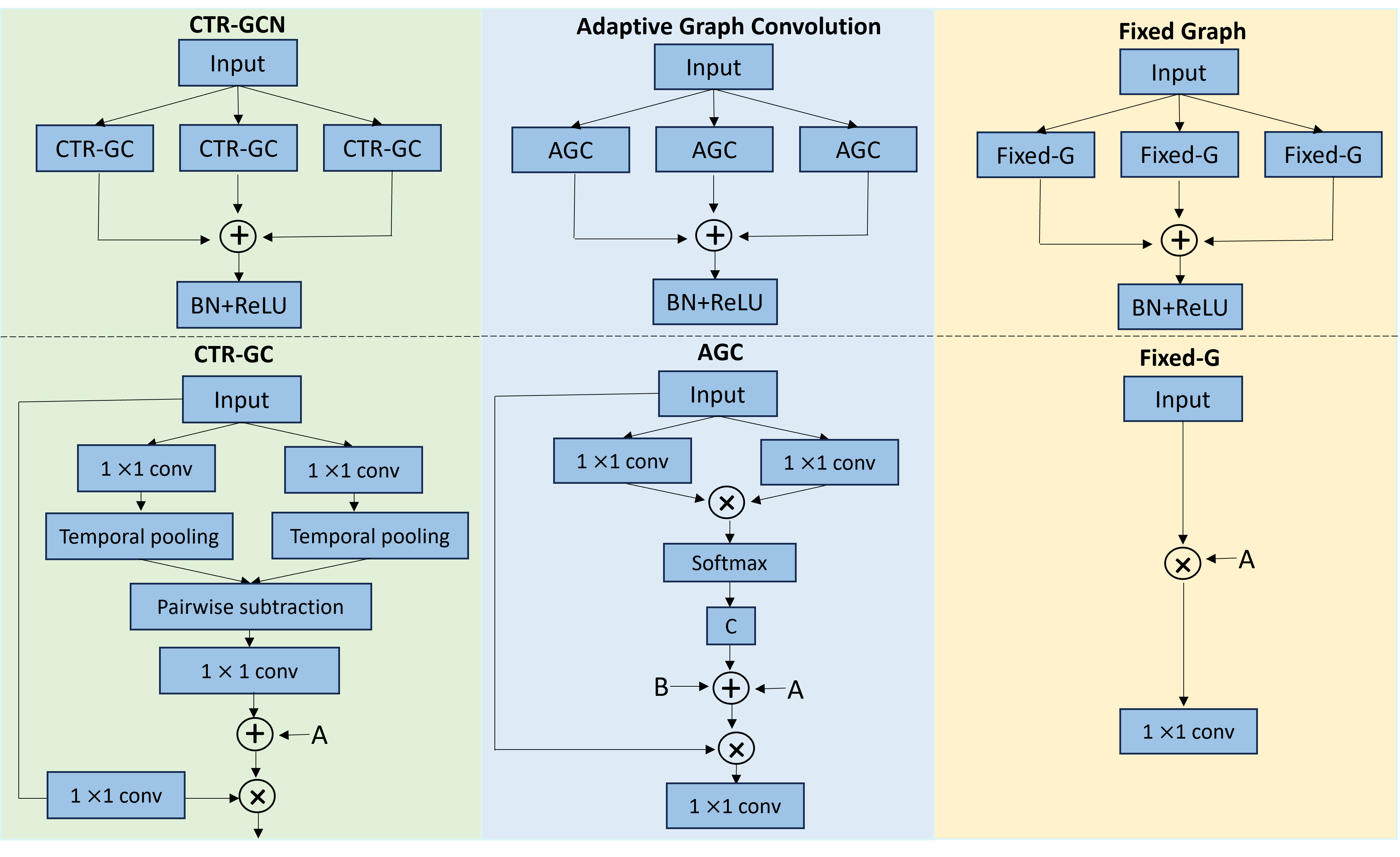
Figure 5: Three GCN Modules used in this paper. The leftmost is CTR-GC module; the middle one is Adaptive graph convolution module; the rightmost is fixed graph as there are no learnable parameters for altering adjacency matrix.

The left part of Figure 5 represents CTR-GC backbone while the middle part describes adaptive graph convolution backbone and the right side is a fixed graph that has no learnable parameters for adjacency matrix. CTR-GC and adaptive graph convolution share some similarities as they both utilise three sub-modules and learn the adjacency matrix from the input data. In contrast, CTR-GCN learn the adjacency matrix for each channel while the channels of adaptive graph convolution shares one same adjacency matrix. Besides, adaptive graph convolution utilise an extra fixed adjacency matrix $B$ representing the physical connection of the body when summing with the learnt adjacency matrix. Different with CTR-GC and adaptive graph convolution, the fixed graph is one of the easiest graphs as there are no learnable parameters for altering the adjacency matrix. As a result, the correlations between joints in the fixed graph are manually defined and remain same all the time.

7.4 Lie Group & Hidden Size Selection

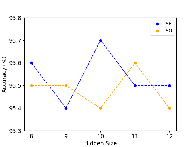
Figure 6: Evaluation across different hidden size in special euclidean (SE) and special orthogonal (SO) Lie group on NTU60-Xview benchmark with the joint stream.

Given that path development constitutes the essence of our methodology, the choice of a suitable Lie Group, along with its corresponding hidden size, significantly influences the ultimate performance of the model. Figure 6 illustrates that a larger hidden size does not necessarily ensure an enhancement in the model and the best result is obtained by utilising the special euclidean group with a hidden size of 10. Note that this result is obtained under the seed 1 and may vary on different seeds and tasks.

7.5 Ablation studies on the initial graph selection

We compare our proposed 3-hop graph representation with I-In-out representations Chen et al. [2021] within the graph module on NTU60 dataset. As we can see from Table 6, employing the 3-hop graph representation yields better performance compared to I-In-Out representations on X-view benchmark while maintaining equal performance on X-sub benchmark.

Table 6: Comparison between the graph using I-In-Out and our proposed 3-hop representation in the GCN module on NTU60 dataset.

Graph Representation	X-sub	X-view
3 Hops (J)	90.8	95.7
I-In-Out (J)	90.8	95.5

7.6 Robustness Analysis

We test the robustness of our approach against the missing frames on NTU60-Xsub benchmark. There are 64 valid frames at the initial stage. We then randomly drop a certain number of frames out of the 64 frames and will have the corresponding $\text{drop rate}=\text{drop frames}/64$. After that, we use linear interpolation based on the remaining frames to fill in the missing frames. We report the accuracy falling number when increasing drop frames/rates at Table 7. As we can see from Table 7, our full model (GCN-DevLSTM) with path development layer always has much less performance degradation compared to CTRGCN Chen et al. [2021] and our model without path development layer (GCN-LSTM). The accuracy rate of our full model only drops 6.07% at a dropping rate reaching 47% while CTR-GCN falls 18.18% and GCN-LSTM falls 16.56%. Our full model with a path development layer demonstrates powerful robustness, benefiting from its theory foundation.

Table 7: Robustness test on NTU60-Xsub benchmark. This table records the accuracy loss when the number of dropping frame increases.

Drop number/rate	GCN-DevLSTM	CTRGCN	GCN-LSTM
0 frames / 0%	0%	0%	0%
5 frames / 8%	-0.85%	-3.01%	-1.39%
10 frames / 16%	-1.35%	-5.38%	-2.12%
15 frames / 23%	-2.04%	-7.01%	-3.46%
20 frames / 31%	-2.99%	-10.19%	-6.23%
30 frames / 47%	-6.07%	-18.18%	-16.56%
40 frames / 63%	-12.93%	-20.65%	-20.31%

References

- Ahmad et al. [2019] Tasweer Ahmad, Lianwen Jin, Jialuo Feng, and Guozhi Tang. Human action recognition in unconstrained trimmed videos using residual attention network and joints path signature. IEEE Access, 7:121212–121222, 2019.
- Boedihardjo et al. [2016] Horatio Boedihardjo, Xi Geng, Terry Lyons, and Danyu Yang. The signature of a rough path: uniqueness. Advances in Mathematics, 293:720–737, 2016.
- Bottou [2012] Léon Bottou. Stochastic gradient descent tricks. In Neural Networks: Tricks of the Trade: Second Edition, pages 421–436. Springer, 2012.
- Cao et al. [2017] Zhe Cao, Tomas Simon, Shih-En Wei, and Yaser Sheikh. Realtime multi-person 2d pose estimation using part affinity fields. In IEEE Conference on Computer Vision and Pattern Recognition, pages 7291–7299, 2017.
- Chen et al. [2021] Yuxin Chen, Ziqi Zhang, Chunfeng Yuan, Bing Li, Ying Deng, and Weiming Hu. Channel-wise topology refinement graph convolution for skeleton-based action recognition. In IEEE International Conference on Computer Vision, pages 13359–13368, 2021.
- Chen [1958] Kuo-Tsai Chen. Integration of paths–a faithful representation of paths by noncommutative formal power series. Transactions of the American Mathematical Society, 89(2):395–407, 1958.
- Cheng et al. [2020a] Ke Cheng, Yifan Zhang, Congqi Cao, Lei Shi, Jian Cheng, and Hanqing Lu. Decoupling gcn with dropgraph module for skeleton-based action recognition. In European Conference on Computer Vision, pages 536–553, 2020.
- Cheng et al. [2020b] Ke Cheng, Yifan Zhang, Xiangyu He, Weihan Chen, Jian Cheng, and Hanqing Lu. Skeleton-based action recognition with shift graph convolutional network. In IEEE Conference on Computer Vision and Pattern Recognition, pages 183–192, 2020.
- Cheng et al. [2023] Jiale Cheng, Dongzi Shi, Chenyang Li, Yu Li, Hao Ni, Lianwen Jin, and Xin Zhang. Skeleton-based gesture recognition with learnable paths and signature features. IEEE Transactions on Multimedia, 2023.
- Chéron et al. [2015] Guilhem Chéron, Ivan Laptev, and Cordelia Schmid. P-cnn: Pose-based cnn features for action recognition. In IEEE International Conference on Computer Vision, pages 3218–3226, 2015.
- Chevyrev and Lyons [2016] Ilya Chevyrev and Terry J Lyons. Characteristic functions of measures on geometric rough paths. Annals of probability: An official journal of the Institute of Mathematical Statistics, 44(6):4049–4082, 2016.
- Driver [1995] BRUCE K Driver. A primer on riemannian geometry and stochastic analysis on path spaces. 1995.
- Du et al. [2015] Yong Du, Wei Wang, and Liang Wang. Hierarchical recurrent neural network for skeleton based action recognition. In IEEE Conference on Computer Vision and Pattern Recognition, pages 1110–1118, 2015.
- Escalera et al. [2013] Sergio Escalera, Jordi Gonzàlez, Xavier Baró, Miguel Reyes, Isabelle Guyon, Vassilis Athitsos, Hugo Escalante, Leonid Sigal, Antonis Argyros, Cristian Sminchisescu, et al. Chalearn multi-modal gesture recognition 2013: grand challenge and workshop summary. In 15th ACM on International conference on multimodal interaction, pages 365–368, 2013.
- Hambly and Lyons [2010] Ben Hambly and Terry Lyons. Uniqueness for the signature of a path of bounded variation and the reduced path group. Annals of Mathematics, pages 109–167, 2010.
- He et al. [2016] Kaiming He, Xiangyu Zhang, Shaoqing Ren, and Jian Sun. Deep residual learning for image recognition. In IEEE Conference on Computer Vision and Pattern Recognition, pages 770–778, 2016.
- Hochreiter and Schmidhuber [1997] Sepp Hochreiter and Jürgen Schmidhuber. Long short-term memory. Neural Comput., 9(8):1735–1780, 1997.
- Kidger et al. [2020] Patrick Kidger, James Morrill, James Foster, and Terry Lyons. Neural controlled differential equations for irregular time series. Advances in Neural Information Processing Systems, 33:6696–6707, 2020.
- Li et al. [2019a] Chenyang Li, Xin Zhang, Lufan Liao, Lianwen Jin, and Weixin Yang. Skeleton-based gesture recognition using several fully connected layers with path signature features and temporal transformer module. In AAAI Conference on Artificial Intelligence, volume 33, pages 8585–8593, 2019.
- Li et al. [2019b] Maosen Li, Siheng Chen, Xu Chen, Ya Zhang, Yanfeng Wang, and Qi Tian. Actional-structural graph convolutional networks for skeleton-based action recognition. In IEEE Conference on Computer Vision and Pattern Recognition, pages 3595–3603, 2019.
- Liao et al. [2019] Lufan Liao, Xin Zhang, and Chenyang Li. Multi-path convolutional neural network based on rectangular kernel with path signature features for gesture recognition. In IEEE Visual Communications and Image Processing (VCIP), pages 1–4. IEEE, 2019.
- Liao et al. [2021] Shujian Liao, Terry Lyons, Weixin Yang, Kevin Schlegel, and Hao Ni. Logsig-rnn: a novel network for robust and efficient skeleton-based action recognition. British Machine Vision Conference, 2021.
- Liu et al. [2017a] Jun Liu, Gang Wang, Ping Hu, Ling-Yu Duan, and Alex C Kot. Global context-aware attention lstm networks for 3d action recognition. In IEEE Conference on Computer Vision and Pattern Recognition, pages 1647–1656, 2017.
- Liu et al. [2017b] Mengyuan Liu, Hong Liu, and Chen Chen. Enhanced skeleton visualization for view invariant human action recognition. Pattern Recognition, 68:346–362, 2017.
- Liu et al. [2018] Jun Liu, Amir Shahroudy, Dong Xu, Alex C Kot, and Gang Wang. Skeleton-based action recognition using spatio-temporal lstm network with trust gates. IEEE Transactions on Pattern Analysis and Machine Intelligence, 40(12):3007–3021, 2018.
- Liu et al. [2019a] Bangli Liu, Haibin Cai, Zhaojie Ju, and Honghai Liu. Rgb-d sensing based human action and interaction analysis: A survey. Pattern Recognition, 94:1–12, 2019.
- Liu et al. [2019b] Jun Liu, Amir Shahroudy, Mauricio Perez, Gang Wang, Ling-Yu Duan, and Alex C Kot. Ntu rgb+d 120: A large-scale benchmark for 3d human activity understanding. IEEE Transactions on Pattern Analysis and Machine Intelligence, 42(10):2684–2701, 2019.
- Liu et al. [2020] Ziyu Liu, Hongwen Zhang, Zhenghao Chen, Zhiyong Wang, and Wanli Ouyang. Disentangling and unifying graph convolutions for skeleton-based action recognition. In IEEE Conference on Computer Vision and Pattern Recognition, pages 143–152, 2020.
- Lou et al. [2022] Hang Lou, Siran Li, and Hao Ni. Path development network with finite-dimensional lie group representation. arXiv preprint arXiv:2204.00740, 2022.
- Lou et al. [2023] Hang Lou, Siran Li, and Hao Ni. Pcf-gan: generating sequential data via the characteristic function of measures on the path space. arXiv preprint arXiv:2305.12511, 2023.
- Lyons and Xu [2017] Terry J Lyons and Weijun Xu. Hyperbolic development and inversion of signature. Journal of Functional Analysis, 272(7):2933–2955, 2017.
- Lyons et al. [2014] Terry Lyons, Hao Ni, and Harald Oberhauser. A feature set for streams and an application to high-frequency financial tick data. In 2014 International Conference on Big Data Science and Computing, pages 1–8, 2014.
- Lyons [1998] Terry J Lyons. Differential equations driven by rough signals. Revista Matemática Iberoamericana, 14(2):215–310, 1998.
- Ni et al. [2021] Hao Ni, Lukasz Szpruch, Marc Sabate-Vidales, Baoren Xiao, Magnus Wiese, and Shujian Liao. Sig-wasserstein gans for time series generation. In Second ACM International Conference on AI in Finance, pages 1–8, 2021.
- Shahroudy et al. [2016] Amir Shahroudy, Jun Liu, Tian-Tsong Ng, and Gang Wang. Ntu rgb+d: A large scale dataset for 3d human activity analysis. In IEEE Conference on Computer Vision and Pattern Recognition, pages 1010–1019, 2016.
- Shi et al. [2019] Lei Shi, Yifan Zhang, Jian Cheng, and Hanqing Lu. Two-stream adaptive graph convolutional networks for skeleton-based action recognition. In IEEE Conference on Computer Vision and Pattern Recognition, pages 12026–12035, 2019.
- Shi et al. [2020] Lei Shi, Yifan Zhang, Jian Cheng, and Hanqing Lu. Skeleton-based action recognition with multi-stream adaptive graph convolutional networks. IEEE Transactions on Image Processing, 29:9532–9545, 2020.
- Si et al. [2019] Chenyang Si, Wentao Chen, Wei Wang, Liang Wang, and Tieniu Tan. An attention enhanced graph convolutional lstm network for skeleton-based action recognition. In IEEE International Conference on Computer Vision, pages 1227–1236, 2019.
- Song et al. [2020] Yi-Fan Song, Zhang Zhang, Caifeng Shan, and Liang Wang. Stronger, faster and more explainable: A graph convolutional baseline for skeleton-based action recognition. In 28th ACM International Conference on Multimedia, pages 1625–1633, 2020.
- Song et al. [2022] Yi-Fan Song, Zhang Zhang, Caifeng Shan, and Liang Wang. Constructing stronger and faster baselines for skeleton-based action recognition. IEEE Transactions on Pattern Analysis and Machine Intelligence, 45(2):1474–1488, 2022.
- Xie et al. [2017] Zecheng Xie, Zenghui Sun, Lianwen Jin, Hao Ni, and Terry Lyons. Learning spatial-semantic context with fully convolutional recurrent network for online handwritten chinese text recognition. IEEE Transactions on Pattern Analysis and Machine Intelligence, 40(8):1903–1917, 2017.
- Xu et al. [2022] Kailin Xu, Fanfan Ye, Qiaoyong Zhong, and Di Xie. Topology-aware convolutional neural network for efficient skeleton-based action recognition. In AAAI Conference on Artificial Intelligence, volume 36, pages 2866–2874, 2022.
- Yan et al. [2018] Sijie Yan, Yuanjun Xiong, and Dahua Lin. Spatial temporal graph convolutional networks for skeleton-based action recognition. In AAAI Conference on Artificial Intelligence, volume 32, 2018.
- Yang et al. [2015] Weixin Yang, Lianwen Jin, and Manfei Liu. Chinese character-level writer identification using path signature feature, dropstroke and deep cnn. In 13th International Conference on Document Analysis and Recognition (ICDAR), pages 546–550. IEEE, 2015.
- Yang et al. [2022] Weixin Yang, Terry Lyons, Hao Ni, Cordelia Schmid, and Lianwen Jin. Developing the path signature methodology and its application to landmark-based human action recognition. In Stochastic Analysis, Filtering, and Stochastic Optimization: A Commemorative Volume to Honor Mark HA Davis’s Contributions, pages 431–464. Springer, 2022.
- Zhao et al. [2019] Rui Zhao, Kang Wang, Hui Su, and Qiang Ji. Bayesian graph convolution lstm for skeleton based action recognition. In IEEE International Conference on Computer Vision, pages 6882–6892, 2019.
- Zhou et al. [2023] Huanyu Zhou, Qingjie Liu, and Yunhong Wang. Learning discriminative representations for skeleton based action recognition. In IEEE Conference on Computer Vision and Pattern Recognition, pages 10608–10617, 2023.