Dipole-dipole interacting two-level emitters in a moderately intense laser field

Abstract

We investigate the resonance fluorescence features of a small ensemble of closely packed and moderately laser pumped two-level emitters at resonance. The mean distance between any two-level radiators is smaller than the corresponding emission wavelength, such that the dipole-dipole interactions are not negligible. We have found that under the secular approximation, the collective resonance fluorescence spectrum consists of $2N+1$ spectral lines, where $N$ is the number of emitters from the sample. The $2N$ lateral spectral-bands, symmetrically located around the generalized Rabi frequency with respect to the central line at the laser frequency, are distinguishable if the dipole-dipole coupling strength is larger than the collective spontaneous decay rate. This way, one can extract the radiators number within the ensemble via measuring of the spontaneously scattered collective resonance fluorescence spectrum. Contrary, if the dipole-dipole coupling is of the order of or smaller than the cooperative spontaneous decay rate, but still non-negligible, the spectrum turns into a Mollow-like fluorescence spectrum, where the two lateral spectral lines broadens, proportional to the dipole-dipole coupling strength, respectively.

I Introduction

Resonance fluorescence of two-level atoms was extensively studied in the scientific literature and significant results were already obtained and reported [1, 2, 3]. An important issue of this research topic is the well-known Mollow spectrum [4] and, probably, there is no need to justify its relevance. It was observed in a wide range of systems, like e.g. atomic beams [5], single molecules [6], quantum dots [7] or cold atoms [8], etc. [9, 10, 11, 12].

When many two-level emitters are considered in the resonance fluorescence phenomena, things can change depending on the mean inter-particle separations [13, 14, 15, 16, 17, 18, 19, 20, 21]. If the atomic ensemble is concentrated in a space volume with linear dimensions smaller than the photon emission wavelength, the collective resonance fluorescence spectrum may consists from multiple spectral lines with higher intensities and various spectral widths, depending on the atomic sizes and external coherent pumping strengths [22, 23, 24, 25, 26, 27, 28, 29, 30]. In this regard, recent experiments include measurements of fluorescence emission spectra of few strongly driven atoms using an optical nanofiber [31], agreeing well with the Mollow spectrum. In a dilute cloud of strongly driven two-level emitters, the Mollow triplet is affected by cooperativity too and exhibits asymmetrical behaviours which were experimentally demonstrated in [32]. Observations of broadening of the spectral line, a small redshift and a strong suppression of the scattered light, with respect to the non-interacting atomic case, in driven dipole-dipole interacting atoms was reported as well, in Ref. [33].

Motivated by recent advances in experimental research dealing with cooperative interactions among many two-level emitters, here we investigate the collective interaction of a small and closely packed ensemble of $N$ two-level emitters with an externally applied coherent laser wave. The inter-particle separations are less than the corresponding emission wavelength, therefore, the dipole-dipole interactions among the two-level radiators are included and can play a relevant role under specific conditions. Particularly, we focus on a situation when the Rabi frequency, arising due to the ensemble interaction with the resonantly applied coherent laser field, is larger than the collective spontaneous decay rate, respectively. On the other hand, it is being commensurable to the dipole-dipole interaction strength, but still bigger. Under these conditions, we have analytically calculated the collective resonance fluorescence spectrum, spontaneously scattered by the laser-driven dipole-dipole interacting two-level radiators, and have found that it consists of $2N+1$ spectral lines. Each of $N$ spectral side-bands are symmetrically generated, with respect to the central spectral line at the laser frequency, around the Rabi frequency, respectively. Furthermore, these spectral side-bands become distinguishable if the dipole-dipole coupling strength is larger than the collective spontaneous decay. In the opposite case, i.e. when the dipole-dipole coupling is similar to or less than the cooperative spontaneous decay rate, the fluorescence spectrum turns into a three-line Mollow-like spectrum, where the spectral widths of the lateral lines broadens, proportional to the dipole-dipole interaction coupling strength. As a possible application of the reported results, one can determine the emitters number by measuring the collective resonance fluorescence spectrum. Alternatively, one can extract the dipole-dipole coupling strength as well as the mean-distance among the closely spaced two-level radiators in a small laser-pumped ensemble, because the frequency interval among the $N$ lateral spectral lines is given by the scaled dipole-dipole coupling, which in turn is inversely proportional to the cubic mean inter-particle separations, respectively. Notice a recent experiment [34], where the laser-driven Dicke model was realized experimentally, and the earlier theoretically predicted non-equilibrium superradiant phase transition in free space, was successfully demonstrated. This makes our findings experimentally achievable in principle.

This paper is organized as follows. In Sec. II we describe the analytical approach and the system of interest, while in Sec. III we calculate the collective resonance fluorescence spectrum spontaneously scattered by laser-pumped two-level emitters. Sec. IV presents and analyses the obtained results. The article concludes with a summary given in Sec. V.

II Theoretical framework

The system of interest consists from an ensemble of externally coherently laser pumped and dipole-dipole interacting $N$ two-level emitters, within the Dicke limit [13]. The Hamiltonian describing this system in the dipole and rotating-wave approximations [14, 15, 16, 17, 18, 19, 20], in a frame rotating at the laser frequency $\omega_{L}$, is as follows:

$$H = \sum_{k}\hbar(\omega_{k}-\omega_{L})a^{\dagger}_{k}a_{k}+\hbar\Delta S_{z}+\hbar\Omega(S^{+}+S^{-})$$ (1)

$$- \hbar\tilde{\delta}S^{+}S^{-}+i\sum_{k}(\vec{g}_{k}\cdot\vec{d})(a^{\dagger}_{k}S^{-}-S^{+}a_{k}),$$

where $\Delta=\omega_{0}-\omega_{L}+\tilde{\delta}$, with $\omega_{0}$ being the emitters transition frequency. The free energies of the environmental electromagnetic field (EMF) vacuum modes and atomic subsystems are given by the first two terms in the Hamiltonian (1). The third and fifth components of the Hamiltonian (1) account for the laser as well as the EMF surrounding vacuum modes interactions with the two-level emitters, respectively. There $\Omega$ is the corresponding Rabi frequency due to the external applied coherent laser field, whereas $\vec{g}_{k}$=$\sqrt{2\pi\hbar\omega_{k}/V}\vec{e}_{p}$ is the coupling strength among the few-level atoms and the EMF vacuum modes. Here $\vec{e}_{p}$ is the photon polarization vector with $p\in\{1,2\}$ and $V$ is the quantization volume. The fourth term describes the dipole-dipole interaction among the two-level emitters, with $\tilde{\delta}=\delta/(N-1)$ being its magnitude. Notice that the Hamiltonian of many atoms is an additive function, i.e. it consists from a sum of individual Hamiltonians, describing separately each two-level emitter. From this reason, the dipole-dipole coupling strength $\delta$ was divided on $N-1$, because there are $N(N-1)$ terms describing the dipole-dipole interacting atoms. Additionally, we have assumed a closely packed atomic ensemble meaning that its linear dimension is much smaller than the photon emission wavelength, $\lambda$, while the dipole-dipole coupling is mainly being proportional to $\delta\sim d^{2}/r^{3}$ [17, 18, 19, 20], where $r$ is the mean distance among any atomic pair characterized by dipole $d$. Further, in the Hamiltonian (1), the collective atomic operators $S^{+}=\sum^{N}_{j=1}|e\rangle_{j}{}_{j}\langle g|$ and $S^{-}=[S^{+}]^{\dagger}$ obey the usual commutation relations for su(2) algebra, namely, $[S^{+},S^{-}]=2S_{z}$ and $[S_{z},S^{\pm}]=\pm S^{\pm}$, where $S_{z}=\sum^{N}_{j=1}(|e\rangle_{j}{}_{j}\langle e|-|g\rangle_{j}{}_{j}\langle g|)/2$ is the bare-state inversion operator. Here, $|e\rangle_{j}$ and $|g\rangle_{j}$ are the excited and ground state of the emitter $j$, respectively, while $a^{\dagger}_{k}$ and $a_{k}$ are the creation and the annihilation operators of the EMF vacuum reservoir which satisfy the standard bosonic commutation relations, i.e., $[a_{k},a^{\dagger}_{k^{\prime}}]=\delta_{kk^{\prime}}$, and $[a_{k},a_{k^{\prime}}]$ = $[a^{\dagger}_{k},a^{\dagger}_{k^{\prime}}]=0$ [14, 15, 16, 17, 18, 19, 20].

Under the action of the laser field, the system is conveniently described using the dressed-state formalism [2, 3]: $|e\rangle_{j}=\cos{\theta}|\tilde{e}\rangle_{j}-\sin{\theta}|\tilde{g}\rangle_{j}$ and $|g\rangle_{j}=\sin{\theta}|\tilde{e}\rangle_{j}+\cos{\theta}|\tilde{g}\rangle_{j}$ with $\cot{2\theta}=\Delta/2\Omega$. The system Hamiltonian (1) can be written then as $H=H_{0}+H_{I}$, where

$$H_{0} = \sum_{k}\hbar(\omega_{k}-\omega_{L})a^{\dagger}_{k}a_{k}+\hbar\bar{G}R_{z}-\hbar\bar{\delta}R^{+}R^{-},$$

$$H_{I} = i\sum_{k}(\vec{g}_{k}\cdot\vec{d})\bigl{\{}a^{\dagger}_{k}(\sin{2\theta}R_{z}/2+\cos^{2}{\theta}R^{-}$$ (2)

$$- \sin^{2}{\theta}R^{+})-H.c.\bigr{\}},$$

with $\bar{G}=G+\tilde{\delta}(\sin^{4}{\theta}-\sin^{2}{2\theta}/2)$, $G=\sqrt{\Omega^{2}+(\Delta/2)^{2}}$ and $\bar{\delta}=\tilde{\delta}(\cos^{4}{\theta}+\sin^{4}{\theta}-\sin^{2}{2\theta})$. Here, in the dipole-dipole part of the Hamiltonian, we have neglected fastly oscillating terms proportional to $e^{\pm ikGt}$, $\{k=2,4\}$, while supposing that $\Omega\gg\tilde{\delta}$, and have used the relation $R^{2}_{z}/4+(R^{+}R^{-}+R^{-}R^{+})/2=j(j+1)$, where $j=N/2$. The new quasispin operators $R^{+}=\sum^{N}_{j=1}|\tilde{e}\rangle_{j}{}_{j}\langle\tilde{g}|$, $R^{-}=[R^{+}]^{\dagger}$ and $R_{z}=\sum^{N}_{j=1}(|\tilde{e}\rangle_{j}{}_{j}\langle\tilde{e}|-|\tilde{g}\rangle_{j}{}_{j}\langle\tilde{g}|)$ operate in the dressed-state picture and obey the commutation relations: $[R^{+},R^{-}]=R_{z}$ and $[R_{z},R^{\pm}]=\pm 2R^{\pm}$. In the interaction picture, given by the unitary transformation $U(t)=\exp{(iH_{0}t/\hbar)}$, one arrives at the interaction Hamiltonian, $H_{i}(t)=U(t)H_{I}U^{-1}(t)$, that is

$$H_{i}(t)=i\sum_{k}(\vec{g}_{k}\cdot\vec{d})a^{\dagger}_{k}\bar{R}^{-}(t)e^{i(\omega_{k}-\omega_{L})t}+H.c.,$$ (3)

where

$$\bar{R}^{-}(t)=\sin{2\theta}R_{z}/2+\cos^{2}{\theta}e^{-i\hat{\omega}t}R^{-}-\sin^{2}{\theta}R^{+}e^{i\hat{\omega}t},$$

with $\hat{\omega}=2\bar{G}+\bar{\delta}R_{z}$ and $\bar{R}^{+}=[\bar{R}^{-}]^{\dagger}$.

The general form of the dressed master equation, in the interaction picture describing the atomic subsystem alone, is given by

$$\frac{d}{dt}\rho(t) + \frac{i}{\hbar}[H_{a},\rho(t)]=$$ (4)

$$- \frac{1}{\hbar^{2}}{\rm Tr_{f}}\biggl{\{}\int^{t}_{0}dt^{\prime}\bigl{[}H_{i}(t),[H_{i}(t^{\prime}),\rho(t^{\prime})]\bigr{]}\biggr{\}},$$

where $H_{a}=\hbar\bar{G}R_{z}-\hbar\bar{\delta}R^{+}R^{-}$, and the notation ${\rm Tr_{f}}\{\cdots\}$ means the trase over the vacuum EMF degrees of freedom. Substituting the Hamiltonian (3) in the above equation (4), after combersome but not difficult calculations, one arrives at the final master equation describing the atomic subsystem only

$$\frac{d}{dt}\rho(t)+\frac{i}{\hbar}[H_{a},\rho(t)]=-\frac{\Gamma_{0}}{8}\sin^{2}{2\theta}[R_{z},R_{z}\rho]$$ (5)

$$- \frac{1}{2}\cos^{4}{\theta}[R^{+},\hat{\Gamma}^{(+)}R^{-}\rho]-\frac{1}{2}\sin^{4}{\theta}[R^{-},R^{+}\hat{\Gamma}^{(-)}\rho]$$

$$+ H.c.,$$

where $\Gamma_{0}=\gamma(\omega_{L})$ and $\hat{\Gamma}^{(\pm)}=\gamma(\omega_{L}\pm\hat{\omega})$ are the spontaneous decay rates, i.e. $\gamma(\omega)=2d^{2}\omega^{3}/(3\hbar c^{3})$, at frequencies $\omega_{L}$ and $\omega_{L}\pm\hat{\omega}$, respectively. Note that we have performed the secular approximation when obtaining Eq. (5), that is, we neglected rapidly oscillating terms proportional to $e^{\pm i\bar{G}t}$, $\{k\in 2,4\}$, meaning generally that $2\bar{G}\gg\{N\gamma(\omega_{L}),\bar{\delta}\}$. One can observe that $\hat{\Gamma}^{(\pm)}\approx\Gamma_{0}\equiv\gamma$, since the eigenvalues of the dressed-state inversion operator vary within $\pm N$ and we consider that $\omega_{L}\gg 2\bar{G}\pm\bar{\delta}N$.

At resonance, when $\Delta=0$ or $\omega_{L}=\omega_{0}+\tilde{\delta}$, one has that $\theta=\pi/4$ and the master equation (5) possesses a steady-state solution

$$\rho_{s}=\frac{\hat{I}}{N+1},$$ (6)

where $\hat{I}$ is the unity operator [18, 22]. We shall use the steady state solution (6) in the next section, when calculating the resonance fluorescence spectrum of dipole-dipole interacting two-level atoms in a moderately intense and coherent laser field.

III The collective resonance fluorescence spectrum

In the far-zone limit, $R=|\vec{R}|\gg\lambda$, one can express the entire steady-state fluorescence spectrum via the collective atomic operators as

$$S(\nu)=\Phi(R){\rm Re}\biggl{\{}\int^{\infty}_{0}d\tau e^{i(\nu-\omega_{L})\tau}\langle S^{+}S^{-}(\tau)\rangle_{s}\biggr{\}},$$ (7)

where the subindex $s$ means steady-state. $\Phi(R)$ is a geometrical factor which we set equal to unity in the following, while $\nu$ is the detected photon frequency. In the dressed-state picture and at resonance, i.e. $\theta=\pi/4$, the fluorescence spectrum transforms as follows in the secular approximation

$$S(\nu) = {\rm Re}\int^{\infty}_{0}d\tau e^{i(\nu-\omega_{L})\tau}\biggl{\{}\langle R_{z}R_{z}(\tau)\rangle_{s}+\langle R^{+}R^{-}(\tau)\rangle_{s}$$ (8)

$$+ \langle R^{-}R^{+}(\tau)\rangle_{s}\biggr{\}}/4.$$

Now, using the master equation (5) one can obtain the time-dependences for the collective dressed-state atomic operators entering in the expression (8) for the resonance fluorescence spectrum, namely,

$$R_{z}(\tau) = R_{z}e^{-\gamma\tau/2},$$

$$R^{-}(\tau) = e^{-(i\hat{\omega}+3\gamma/4)\tau}R^{-},$$

$$R^{+}(\tau) = R^{+}e^{(i\hat{\omega}-3\gamma/4)\tau},$$ (9)

reminding that $\hat{\omega}=2\Omega-\tilde{\delta}(1+R_{z})/2$, if $\theta=\pi/4$. Inserting the time-solutions (9) in (8) and performing the integration, one arrives at the following exact expression for the steady-state collective resonance fluorescence spectrum

$$S(\nu) = \frac{1}{4}\biggl{\{}\sum_{\pm}\sum^{N}_{n=0}I^{(\pm)}_{n}\frac{3\gamma/4}{\bigl{(}3\gamma/4\bigr{)}^{2}+\bigl{(}\nu-\omega^{(\pm)}_{n}\bigr{)}^{2}}$$ (10)

$$+ I_{0}\frac{\gamma/2}{\bigl{(}\gamma/2\bigr{)}^{2}+\bigl{(}\nu-\omega_{L}\bigr{)}^{2}}\biggr{\}},$$

where the symbol $\sum_{\pm}$ indicates that both sets of spectral lines appearing with the plus sign and with the minus sign need to be incorporated in the sum. There, $I_{0}=N(N+2)/3$, $I^{(+)}_{n}=n(N-n+1)/\bigl{(}N+1\bigr{)}$, $I^{(-)}_{n}=(n+1)(N-1)/\bigl{(}N+1\bigr{)}$ and $\omega^{(\pm)}_{n}$ = $\omega_{L}\pm 2\Omega\mp\tilde{\delta}(2n-N\mp 1)/2$, respectively. Note that the collective resonance fluorescence spectrum, given by the expression (10), is valid under the secular approximation, i.e. $2\Omega\gg N\gamma$, as well as for $\delta/(2\Omega)<1$.

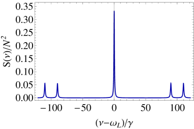
Figure 1: The scaled collective resonance fluorescence spectrum $S({\nu})/N^{2}$ as a function of $(\nu-\omega_{L})/\gamma$. Here $N=2$, $2\Omega/\gamma=100$, $\Delta/\gamma=0$, and $\delta/(2\Omega)=0.2$, respectively.

In order to calculate the corresponding collective dressed-state correlators entering in the expression for resonance fluorescence spectrum, after inserting (9) in (8), we considered an atomic coherent state $|n\rangle$, which is a symmetrized $N$-atom state with $N–n$ particles in the lower dressed state $|\tilde{g}\rangle$ and $n$ atoms excited to the upper dressed state $|\tilde{e}\rangle$. We can calculate then the steady-state expectation values of any atomic correlators of interest, for $\theta=\pi/4$, using the steady-state solution (6) of the maser equation (5) as well as the relations: $R^{+}|n\rangle=\sqrt{(N-n)(n+1)}|n+1\rangle$, $R^{-}|n\rangle=\sqrt{n(N-n+1)}|n-1\rangle$ and $R_{z}|n\rangle=(2n-N)|n\rangle$. Particularly, if the dipole-dipole interactions are ignored, i.e. $\delta/2\Omega\to 0$, then one obtains the well-known expression for the collective resonance fluorescence spectrum in this case, see e.g. [22, 23, 24],

$$S(\nu) = \frac{1}{4}\biggl{\{}\sum_{\pm}I^{(\pm)}\frac{3\gamma/4}{\bigl{(}3\gamma/4\bigr{)}^{2}+\bigl{(}\nu-\omega_{L}\mp 2\Omega\bigr{)}^{2}}$$ (11)

$$+ I_{0}\frac{\gamma/2}{\bigl{(}\gamma/2\bigr{)}^{2}+\bigl{(}\nu-\omega_{L}\bigr{)}^{2}}\biggr{\}},$$

where $I^{\pm}=N(N+2)/6$. Again here the symbol $\sum_{\pm}$ indicates that there are two spectral lines, one appearing with the plus sign and another one with the minus sign, respectively. The resonance fluorescence spectrum (11) turns into the famous single-atom Mollow spectrum [4], if one sets $N=1$, with the central- and side-bands spectral widths equal to $\gamma/2$ and $3\gamma/4$, respectively. Finally, in both cases, that is for the ratio $\delta/2\Omega\not=0$ but smaller than unity, or $\delta/2\Omega\to 0$, the collective resonance fluorescence spectra, i.e. the expressions (10) and (11), are proportional to the squared number of involved two-level emitters, i.e. $S(\nu)\propto N^{2}$.

In the following section, we shall discuss the collective resonance fluorescence spectrum, given by the expression (10), of a collection of closely packed and dipole-dipole interacting two-level emitters driven by a moderately intense and resonant coherent laser field.

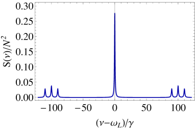
Figure 2: Same as in Fig. (1), but for $N=3$.

IV Results and Discussion

While for $\delta/2\Omega\to 0$ we have obtained that the collective resonance fluorescence spectrum consists from three-spectral lines, similar to the Mollow spectrum, things are different if $\delta/2\Omega\not=0$, so that $\delta/2\Omega<1$, as it is the case discussed here. Actually, additional spectral side-bands appear which are centered around $\omega_{L}\pm 2\Omega$. Evidently, this occurs due to the dipole-dipole interaction among the two-level emitters. In this context, Fig. (1) shows the resonance fluorescence spectrum for a two-atom system, in the Dicke limit, i.e. the space-interval between the two atoms is much smaller than the corresponding photon emission wavelength, but with the dipole-dipole interaction taken into account, respectively. The spectrum consists from symmetrically located five spectral lines at $\nu=\omega_{L}$ and $\nu-\omega_{L}=\pm 2\Omega\pm\delta/2$, see also [25, 26, 27, 28]. The frequency interval among the two spectral-lines, around $\nu-\omega_{L}=\pm 2\Omega$, equals the dipole-dipole coupling strength $\delta$. An explanation of the resonance fluorescence spectrum given in Fig. (1) can be done using the double-dressed state formalism: The laser-emitter dressed states $|\tilde{e}\rangle_{j}$ and $|\tilde{g}\rangle_{j}$ additionally split due to the dipole-dipole interaction leading to the collective two-atom dressed-states, see e.g. [35], which are responsible for the spontaneously emitted spectrum. On the other side, Fig. (2) depicts the fluorescence spectrum of resonantly driven $N=3$ two-level emitters, also for $\Delta/\gamma=0$ and within the Dicke-limit with dipole-dipole interaction being included, respectively. This time, the spectrum consists of seven spectral lines detected, correspondingly, at $\nu=\omega_{L}$, $\nu=\omega_{L}\pm 2\Omega$ and $\nu-\omega_{L}=\pm 2\Omega\pm\delta/2$. Again, here, the three-spectral lines around $\nu-\omega_{L}=\pm 2\Omega$ are localized within the dipole-dipole coupling strength $\delta$, see Fig. (2). In the same vein, a $N=7$ resonantly pumped two-level sample generates 15 spectral lines. The fluorescence spectrum is symmetrically located with respect to the central line at $\nu=\omega_{L}$, see Fig. (3). Each seven spectral side-bands are generated around $\nu-\omega_{L}=\pm 2\Omega$ in a frequency range equal to the dipole-dipole coupling $\delta$.

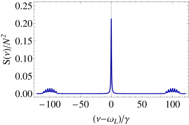
Figure 3: Same as in Fig. (1), but for $N=7$.

Generalizing, one can observe that the cooperative resonance fluorescence spectrum of a moderately laser driven small two-level ensemble, within the Dicke-limit with dipole-dipole interaction included, consists of $2N+1$ spectral lines. A central line at $\nu=\omega_{L}$, and $2N$ spectral lines symmetrically generated around the frequencies $\nu-\omega_{L}=\pm 2\Omega$, respectively. Remarkably here, one can extract the number of involved two-level emitters via detection of the collective resonance fluorescence spectrum, because both lateral side-bands consists from $N$ spectral lines. The frequency separation among these $N$ spectral lines, each generated on both sides of the spectrum with respect to the central line at $\nu=\omega_{L}$, is equal to $\delta/(N-1)$. These lines are distinguishable if $\delta/(N-1)\gg\gamma$ when $\Delta/\gamma=0$ or, equivalently, $\omega_{L}\equiv\omega_{0}+\tilde{\delta}$. Knowing the dipole-dipole coupling strength from the spectrum, one can extract the mean-distance among the closely spaced two-level radiators, because the dipole-dipole interaction scales inversely proportional to the cubic mean inter-particle separations, respectively, see also [36].

Larger atomic ensembles, with a fixed ratio of $2\Omega/N\gamma\gg 1$, lead to a three spectral-line Mollow spectrum, where the two lateral side-bands, generated at $\nu=\omega_{L}\pm 2\Omega$, broadens if $\delta/(N-1)\sim\gamma$ or less, see Fig. (4). Then the frequency bandwidth of the two lateral spectral lines, located at $\nu=\omega_{L}\pm 2\Omega$ in the Mollow like-spectrum, is close to the dipole-dipole coupling strength, $\delta$, as shown in Fig. (4). In order to fulfil the secular approximation, i.e. $2\Omega\gg N\gamma$, in Fig. (4), we took $2\Omega/\gamma=200$, meaning higher applied field intensities with respect to previous cases, where one has $2\Omega/\gamma=100$. Notice that the broadening of the lateral spectral line-widths of the Mollow spectrum, but in a regular sub-wavelength chain of laser pumped dipole-dipole interacting two-level atoms [37], was recently reported as well, in Ref. [38].

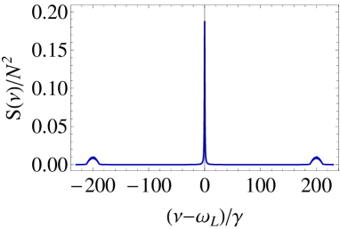
Figure 4: Same as in Fig. (1), but for $N=15$, $2\Omega/\gamma=200$, and $\delta/2\Omega=0.1$.

V Conclusions

We have investigated the collective steady-state quantum dynamics of an externally resonantly pumped two-level ensemble, concentrated in a small volume within the Dicke limit and secular approximation. However, the dipole-dipole interactions among the emitters are taken into account, while their coupling strength is considered to be of the order of the corresponding Rabi frequency, but still smaller. As a result, we have found that the collective resonance fluorescence spectrum consists of multiple spectral lines which are dependent on ensemble’s sizes. As a consequence, one can determine the number of involved emitters via measuring the spontaneously scattered resonance fluorescence spectrum. This is feasible since the number of the lateral spectral bands equals to the doubled number of two-level radiators within the laser-pumped sample. Actually, the lateral spectral lines are distinguishable if the dipole-dipole coupling is larger than the collective spontaneous decay rate. In the opposite case, the collective resonance fluorescence spectrum is formed from three lines, similar to the Mollow spectrum, whereas the lateral spectral lines broadens proportional to the dipole-dipole coupling strength, respectively. In both case, one can extract the dipole-dipole coupling strength as well as the mean-distance among the closely spaced laser-driven two-level emitters.

- [1] H. Walther, Resonance fluorescence of two-level atoms, Advances in Atomic, Molecular and Optical Physics 51, 239, (2005); and references therein.
- [2] C. Cohen-Tannoudji, Atoms in Electromagnetic Fields, (World Scientific, London, 1994).
- [3] M. O. Scully and M. S. Zubairy, Quantum Optics (Cambridge University Press, Cambridge, U.K., 1997).
- [4] B. R. Mollow, Power Spectrum of Light Scattered by Two-Level Systems, Phys. Rev. 188, 1969 (1969).
- [5] F. Y. Wu, R. E. Grove, and S. Ezekiel, Investigation of the Spectrum of Resonance Fluorescence Induced by a Monochromatic Field, Phys. Rev. Lett. 35, 1426 (1975).
- [6] G. Wrigge, I. Gerhardt, J. Hwang, G. Zumofen, and V. Sandoghdar, Efficient coupling of photons to a single molecule and the observation of its resonance fluorescence, Nature Physics 4, 60 (2008).
- [7] A. Ulhaq, S. Weiler, S. M. Ulrich, R. Robach, M. Setter, and P. Michler, Cascaded single-photon emission from the Mollow triplet sidebands of a quantum dot, Nature Photonics 6, 238 (2012).
- [8] L. O.-Gutiérrez, R. C. Teixeira, A. Eloy, D. Ferreira da Silva, R. Kaiser, R. Bachelard, and M. Fouché, Mollow triplet in cold atoms, New J. Phys. 21, 093019 (2019).
- [9] S. G. Rautian, and I. I. Sobel’man, Line shape and dispersion in the vicinity of an absorption band, as affected by induced transitions, Sov. Phys. JETP 14, 328 (1962).
- [10] J. Berney, M. T. Portella-Oberli, and B. Deveaud, Dressed excitons within an incoherent electron gas: Observation of a Mollow triplet and an Autler-Townes doublet, Phys. Rev. B 77, 121301(R) (2008).
- [11] O. Postavaru, Z. Harman, and C. H. Keitel, High-Precision Metrology of Highly Charged Ions via Relativistic Resonance Fluorescence, Phys. Rev. Lett. 106, 033001 (2011).
- [12] M. A. Antón, S. Maede-Razavi, F. Carreo, I. Thanopulos, and E. Paspalakis, Optical and microwave control of resonance fluorescence and squeezing spectra in a polar molecule, Phys. Rev. A 96, 063812 (2017).
- [13] R. H. Dicke, Coherence in Spontaneous Radiation Processes, Phys. Rev. 93, 99 (1954).
- [14] G. S. Agarwal, Quantum Statistical Theories of Spontaneous Emission and their Relation to Other Approaches (Springer, Berlin, 1974).
- [15] M. Gross, and S. Haroche, Superradiance: An essay on the theory of collective spontaneous emission, Phys. Rep. 93, 301 (1982).
- [16] A. V. Andreev, V. I. Emel’yanov, and Y. A. Il’inskii, Cooperative Effects in Optics: Superfluorescence and Phase Transitions (IOP, London, 1993).
- [17] J. Peng and G.-X. Li, Introduction to Modern Quantum Optics (World Scientific, Singapore, 1998).
- [18] R. R. Puri, Mathematical Methods of Quantum Optics (Springer, Berlin, 2001).
- [19] Z. Ficek and S. Swain, Quantum Interference and Coherence: Theory and Experiments (Springer, Berlin, 2005).
- [20] M. Kiffner, M. Macovei, J. Evers, and C. H. Keitel, Vacuum-induced processes in multilevel atoms, Progress in Optics 55, 85 (2010).
- [21] B. W. Adams, Ch. Buth, S. M. Cavaletto, J. Evers, Z. Harman, Ch. H. Keitel, A. Pálffy, A. Picon, R. Röhlsberger, Y. Rostovtsev, and K. Tamasaku, X-ray quantum optics, J. Mod. Opt. 60, 2 (2013).
- [22] G. S. Agarwal, L. M. Narducci, D. H. Feng, and R. Gilmore, Phys. Rev. Lett. 42, 1260 (1979).
- [23] G. Compagno, and F. Persico, Theory of collective resonance fluorescence in strong driving fields, Phys. Rev. A 25, 3138 (1982).
- [24] T. Quang, M. Kozierowski, and L. H. Lan, Collective resonance fluorescence in a squeezed vacuum, Phys. Rev. A 39, 644 (1989).
- [25] S. J. Kilin, Cooperative resonance fluorescence and atomic interactions, J. Phys. B: Atom. Molec. Phys. 13 2653 (1980).
- [26] H. S. Freedhoff, Collective atomic effects in resonance fluorescence: The ”scaling factor”, Phys. Rev. A 26, 684 (1982).
- [27] T. Weihan, and G. Min, Resonance fluorescence in a many-atom system, Phys. Rev. A 34, 4070 (1986).
- [28] A. Joshi, and R. R. Puri, The transient fluorescence spectrum of a strongly driven two-atom Dicke model including dipole interaction in a squeezed vacuum, Opt. Commun. 86, 469 (1991).
- [29] M. Macovei, J. Evers, and C. H. Keitel, Coherent manipulation of collective three-level systems, Phys. Rev. A 71, 033802 (2005).
- [30] R. Jones, R. Saint, and B. Olmos, Far-field resonance fluorescence from a dipole interacting laser-driven cold atomic gas, J. Phys. B: At. Mol. Opt. Phys. 50, 014004 (2017).
- [31] M. Das, A. Shirasaki, K. P. Nayak, M. Morinaga, Fam Le Kien, and K. Hakuta, Measurement of fluorescence emission spectrum of few strongly driven atoms using an optical nanofiber, Optics Express 18, 17154 (2010).
- [32] J. R. Ott, M. Wubs, P. Lodahl, N. A. Mortensen, and R. Kaiser, Cooperative fluorescence from a strongly driven dilute cloud of atoms, Phys. Rev. A 87, 061801(R) (2013).
- [33] J. Pellegrino, R. Bourgain, S. Jennewein, Y. R. P. Sortais, A. Browaeys, S. D. Jenkins, and J. Ruostekoski, Observation of Suppression of Light Scattering Induced by Dipole-Dipole Interactions in a Cold-Atom Ensemble, Phys. Rev. Lett. 113, 133602 (2014).
- [34] G. Ferioli, A. Glicenstein, I. Ferrier-Barbut, and A. Browaeys, A non-equilibrium superradiant phase transition in free space, Nature Physics 19, 1345 (2023).
- [35] M. Macovei, and C. H. Keitel, Laser Control of Collective Spontaneous Emission, Phys. Rev. Lett. 91, 123601 (2003).
- [36] J.-T. Chang, J. Evers, M. O. Scully, and M. S. Zubairy, Measurement of the separation between atoms beyond diffraction limit, Phys. Rev. A 73, 031803(R) (2006).
- [37] M. Reitz, C. Sommer, and C. Genes, Cooperative Quantum Phenomena in Light-Matter Platforms, Phys. Rev. X Quantum 3, 010201 (2022).
- [38] O. Scarlatella, and N. R. Cooper, Fate of the Mollow triplet in strongly-coupled atomic arrays, arXiv: 2403.03679v1 [cond-mat.quant-gas], (2024).