Forecasting the load of Parcel Pickup Points
using a Markov Jump Process

Abstract

The growth of e-commerce has resulted in a surge in parcel deliveries, increasing transportation costs and pollution issues. Alternatives to home delivery have emerged, such as the delivery to so-called parcel pick-up points (PUPs), which eliminates delivery failure due to customers not being at home. Nevertheless, parcels reaching overloaded PUPs may need to be redirected to alternative PUPs, sometimes far from the chosen ones, which may generate customer dissatisfaction. Consequently, predicting the PUP load is critical for a PUP management company to infer the availability of PUPs for future orders and better balance parcel flows between PUPs.

This paper proposes a new approach to forecasting the PUP load evolution using a Markov jump process that models the parcel life cycle. The latest known status of each parcel is considered to estimate its contribution to the future load of its target PUP. This approach can account for the variability of activity, the various parcel preparation delays by sellers, and the diversity of parcel carriers that may result in different delivery delays. Here, results are provided for predicting the load associated with parcels ordered from online retailers by customers (Business-to-Customer, B2C). The proposed approach is generic and can also be applied to other parcel flows to PUPs, such as second-hand products (Customer-to-Customer, C2C) sent via a PUP network.

1 Introduction

The recent surge in e-commerce, mostly from online retailers to consumers (Business to Customer, B2C) [1], has led to a substantial rise in parcel deliveries. This increase has implications for both transportation costs and environmental pollution. Furthermore, in case no one (neither customers, neighbors nor a concierge) is present to accept parcels, this results in failed delivery, necessitating multiple rescheduling attempts. In such situations, the distance covered by delivery services in increased substantially [2].

Alternative delivery services have been implemented, especially for the last-mile delivery, i.e., the delivery process between the last dispatch center of the carrier and the final customer. Customers can choose to have their parcels delivered at a post office, or at a pick-up point (PUP) close to their home or their workplace [3]. PUP Management Companies (PMCs) offer two types of PUPs [4]: i) automatic parcel lockers (APL) [5], usually installed within train stations, supermarkets, or ii) local shops (such as food stores or corner shops). This delivery service presents multiple advantages, including a wider range of opening hours compared to that of post offices for customers to pick up their parcels, as well as additional customer visits and income for local shops serving as PUPs [4]. Finally, it is also a sustainable solution for reducing transportation fees and limiting delivery failures compared to traditional home delivery [6]. Customers can also drop off parcels at these PUPs in case of product returns or when they sell new or used products to other customers (C2C service).

Managing a PUP network comes with several challenges. When the chosen PUP is overloaded, customers may find their parcels delivered at a different PUP, sometimes far from their intended pick-up location, leading to customer dissatisfaction. Local shops serving as PUPs may sometimes receive too many parcels for their storage capacity. The parcel management activity may then be detrimental to their primary activity, especially when some parcels have not been accepted and have been re-routed to an alternative PUP. Some other PUPs do not handle enough parcels to benefit from the PUP activity. These are the two main reasons for contract cancellation betwen PUPs and PMCs.

Consequently, the PMCs have to monitor and control the load of each PUP carefully in order to better balance parcel loads among neighboring ones. PUPs likely to be overloaded in the coming days will not be offered to customers during the ordering process. To achieve this, predicting the load of a given PUP several days in advance is essential for PMCs to manage their PUP network more effectively.

Our previous paper [7] describes forecasting approaches for the load associated with the Business-to-Customer (B2C) process by considering the load evolution as a time series. This approach makes it difficult to account for the variability of sellers and of carriers, which may introduce a large diversity of parcel preparation and delivery delays. In this work, we model the latency between statuses for each parcel rather than estimating the number of parcels in each status, as done in [7]. We assume that each parcel runs through a non-stationary Markov chain where the states represent the different statuses the parcel can take on. By doing so, we can deduce the probability distribution of the load at each instant, which is a critical information for PMC decisions regarding the availability of PUPs for future orders. The temporal variability of the activity (peaks during sales or before Christmas), as well as the diversity of sellers and carriers are then easier to take into account. Moreover, the adopted approach is generic and allows for different status flowcharts on the part of the PMCs, and provides a much larger modeling flexibility compared to [7]. We subsequently apply this approach to a specific scenario.

The remainder of the paper is organized as follows. Section 2 presents some related works. Section 3 details and formalizes the PUP load forecasting problem. Section 4 describes the load forecasting approach. The considered prediction approach is compared with alternative ones in terms of prediction accuracy in Section 6. Conclusions and perspectives are provided in Section 7.

Table 1 introduces the main notations used in this paper.

Notation	Variables
$\tau$	Parcel identifier
$\rho$	PUP identifier
$T$	Time sampling period
$k$	Time interval index
$H_{0}$	Necessary time to prepare the order for expedition
$H_{n}$	Holding time for a transition between two intermediate state
$\mathcal{R}$	The set of retailers
$\Gamma$	The set of available carriers
$\mathcal{S}$	The set of status
At time $k$
$w\left(k\right)$	the day of the week of the time interval $k$
$h$$\left(k\right)$	the hour of the day of time $k$
$\mathcal{P}_{k}$	set of parcel indexes with information available with any PUP as target
$\mathcal{P}_{k}^{\rho}$	set of parcel indexes with information available with PUP $\rho$ as target
$\mathbb{V}_{k}$	set of virtual parcel indexes (since not known at time $k$)
$\Lambda_{\tau}\left(k\right)$	variable indicating whether $\tau$ contributes to the load of PUP $\rho$
$L\left(k\right)$	number of parcels in target PUP
$O\left(k\right)$	number of orders that will be confirmed at time $k$
For parcel $\tau$
$R(\tau)$	bought from the retailer $R$
$C(\tau)$	carrier in charge of the delivery
$S_{k}\left(\tau\right)$	current status during time interval $k$
$T_{S_{k}}\left(\tau\right)$	first time interval at which status has switched to $S_{k}$
$H_{n}$	holding time in status $n$
Sets of identifiers of parcels expected to contribute to target PUP load at time $k+j$
$\mathcal{L}_{N}\left(k+j\mid k\right)$	parcels known to be delivered (status $N-1$) before time $k$, and expected to be still waiting to be picked-up at time $k+j$
$\mathcal{L}_{n}\left(k+j\mid k\right)$	parcels with known status $n-1$ before time $k$, and which expected to be delivered before time $k+j$
$\mathcal{L}_{0}\left(k+j\mid k\right)$	parcels containing products not yet ordered at time $k$, but which are expected to be waiting to be picked-up at time $k+j$

Table 1: Main notations

2 Related work

The development of last-mile delivery raises multiple difficulties [8, 9], such as customer desires for shorter delivery delays, seasonal peaks of parcels [10], optimal deployment of PUP locations [11], etc.

While the limited-capacity issue of APLs has been identified in [12], the load of PUPs has not been studied in detail, although this aspect needs to be controlled by the PMCs in order to limit delivery failures. The PUP parcel load prediction consists of the evaluation of the parcel preparation and transportation delays once a product has been ordered, and the prediction of the pick-up delay by the e-customer once the parcel has been delivered to the PUP.

Several works have proposed prediction approaches for e-commerce activity. In [13], statistical and computational intelligence methods are put at work using demand data of a furniture company. A multi-layer LSTM model is employed and compared to alternative techniques. A data mining approach is proposed [14] for online clothing sales forecasting. Seasons, sales, and holidays are identified as essential factors of demand in [15]. The time-series forecasting library Prophet [16] and support vector regression models [17] are combined in [18] to forecast time series demand in the manufacturing industry accounting for seasonality.

Regarding the delivery delay estimation, [19] proposes a real-time forecasting approach of the delivery time based on relevant operational features, including the time of order, the distribution center that will be used, the order, and the user. Concerning the pick-up delay, a statistical analysis in [20] shows that more than $60$ % of the parcels are collected less than 24 hours after delivery, and about $75$ % are collected in less than 48 hours, with considerable regional variations.

While the prediction of each of these aspects (amount of sales, delivery delays, and pick-up delays) have been studied separately, there is a gap in the literature as far as a combined analysis is concerned which forms the subject of this paper. Similar multi-faceted forecasting problems can also be identified for the load evaluation of an intermediate warehouse, where the duration between the delivery and the pick-up process has to be evaluated [21].

In this paper, we extensively use Markov models [22], frequently employed to describe systems with discrete state transitions, assuming (for first-order models) that the transition probabilities only depend on the current state of the system. Considering the life cycle of parcels, transition probabilities from a given state evolve with time. In our study, factors determining the state transition probabilities of a parcel at each time instant are primarily the current state, the day of the week, and the hour of the last transition. These characteristics are closer to a non-homogeneous (or non-stationary) Markov model, as described in [23], where the transition probabilities depend not only on the current state but also on the current time instant. Other particularities of our process are the transitions to one direction only, see Figure 1, and the maximum sojourn time of each parcel after delivery. Therefore we consider a non-stationary Markov model taking into account all these characteristics, which will be developed in Section 3.

3 Problem description

This section models the life-cycle of a parcel starting from its order confirmation on the website of an online retailer (classical or second-hand) and ending with its pickup by a customer in the target PUP. The transitions between the various parcel states are described by a Markov jump process. Finally, the PUP load forecasting problem is formalized.

3.1 Model of the life-cycle of a parcel

Time is sampled with a period of $T$ (typically one hour). Let $k\in\mathbb{N}$ be the index of the time interval $\left[kT,\left(k+1\right)T\right[$. The day of the week of the time interval $k$ is $w\left(k\right)\in\left[1,7\right]$, from Monday ($w\left(k\right)=1$) to Sunday ($w\left(k\right)=7$). The hour of the day at which the interval $\left[kT,\left(k+1\right)T\right[$ starts is $h\left(k\right)\in\left[0,24\right[$.

Consider a parcel with index $\tau$ bought from an online retailer $R\left(\tau\right)\in\mathcal{R},$ where $\mathcal{R}$ is the set of retailers. A carrier $C\left(\tau\right)\in\Gamma$ is in charge of the delivery of the parcel to some target PUP $\rho$, where $\Gamma$ is the set of available carriers. The evolution of the state of parcel $\tau$ is represented by the sequence of random pairs $\left\{\left(S_{k}\left(\tau\right),T_{S_{k}}\left(\tau\right)\right)\right\}_{k\in\mathbb{N}}$, where $S_{k}\left(\tau\right)\in\mathcal{S}=\left\{0\dots N\right\}$ indicates the status of the parcel $\tau$ in the time interval $k$ and

$$T_{S_{k}}\left(\tau\right)=\min\left\{\ell\,|\,S_{\ell}\left(\tau\right)=S_{k}\left(\tau\right)\right\}$$ (1)

represents the index of the time interval at which the parcel has switched to status $S_{k}\left(\tau\right)$. If $S_{k+1}=S_{k}$ then $T_{S_{k+1}}=T_{S_{k}}$. If $S_{k+1}\neq S_{k}$ then $T_{S_{k+1}}=k+1$. Consequently, there is a minimum delay of $T$ between consecutive transitions. When the order is confirmed, the parcel is in status $S=0$. Parcels with status $S=N-1$ have been delivered to the PUP. Finally, the status $S=N$ corresponds to a parcel picked-up by the customer or returned to the retailer. All intermediate statuses between $1$ and $N-2$ correspond to the product wrap-up, collection at the retailer warehouse, and processing at the intermediate logistic platforms of the carrier.

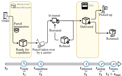
The transitions between these statuses are presented in Figure 1. We assume that the sequence of states of the parcel $\left\{\left(S_{k},T_{S_{k}}\right)\right\}_{k\in\mathbb{N}}$ satisfies the Markov property

$$\mathbb{P} \left(\left(s_{k+1},t_{s_{k+1}}\right)\mid\left(s_{k},t_{s_{k}}\right),\dots,\left(s_{1},t_{s_{1}}\right)\right)$$

$$=\mathbb{P}\left(\left(s_{k+1},t_{s_{k+1}}\right)|\left(s_{k},t_{s_{k}}\right)\right).$$

For all $n\in\mathcal{S}$, $n<N$, the holding time of parcel $\tau$ in status $n$ is

$$H_{n}=T_{n+1}-T_{n}.$$ (2)

Figure 1: Statuses and possible transitions between statuses for a parcel; From time $k$ to $k+1$, the parcel can stay in status $n$ or switch to the status $n+1$; When the status $N$ is reached (picked-up parcel), parcels stay in this status and do not contribute to the PUP load anymore.

The probability for parcel $\tau$ to switch to state $\left(n+1,t_{n+1}\right)$, $t_{n+1}-t_{n}$ time slots after having entered state $\left(n,t_{n}\right)$ at time $t_{n}<t_{n+1}$ depends on several parameters, such as the time $T_{n}=t_{n}$, the online retailer $R$, the carrier $C$, and the target PUP $\rho$. In the most general case, for $0\leqslant n<N$, one has

$$\mathbb{P} \left(T_{n+1}=t_{n+1}\mid T_{n}=t_{n},R=r,C=c,\rho\right)$$

$$=\mathbb{P}\left(H_{n}=t_{n+1}-t_{n}\mid T_{n}=t_{n},R=r,C=c,\rho\right)$$

$$=f_{n}\left(t_{n+1}-t_{n}\mid t_{n},r,c,\rho\right).$$ (3)

Nevertheless, for a given status $n$, the transition probability in (3) may depend only on a reduced subset of parameters.

For example, if status $S=1$ corresponds to a parcel wrapped up and ready to be taken over at the retailer warehouse, the holding time $H_{0}$ represents the time necessary to prepare the order for expedition. This time depends only on the retailer $R=r$ and on the order confirmation time $T_{0}=t_{0}$. One may further assume that $H_{0}$ only depends on the day of the week $w\left(t_{0}\right)$ and the hour of the day $h\left(t_{0}\right)$ of the order confirmation. Once a parcel has been taken over by a carrier $C=c$, the following holding times do not depend any more on the retailer. Consequently, for a transition between two intermediate states $\left(n,t_{n}\right)$ to $\left(n+1,t_{n+1}\right)$ with $n>1$ and $n+1<N$ during the parcel transportation, the holding time $H_{n}$ depends mainly on the carrier $C=c$, as well as the day of the week $w\left(t_{n}\right)$ and the hour of the day $h\left(t_{n}\right)$ of the status $n$. The time of delivery to the PUP $T_{N-1}=t_{N-1}$ depends on the carrier $C=c$, the day of the week $w\left(t_{N-2}\right)$ and the hour of the day $h\left(t_{N-2}\right)$ of the status $N-2$, and on the PUP $\rho$ (parcel are delivered to PUPs every day, except Sundays over a relatively short time interval of the day, depending on the tour of the carrier).

Accounting for fewer parameters in the expression of $f_{n}$ facilitates its estimation from historical data. In what follows, the dependency of $f_{n}$ in $r$, $c$, or $\rho$ is omitted to lighten notations.

3.2 Problem formulation

A parcel $\tau$ contributes to the load of PUP $\rho$ at time $k$ if $S_{k}\left(\tau\right)=N-1$, i.e., if $T_{N-1}\left(\tau\right)\leqslant k$ (it has been delivered to the PUP before time $k$) and $T_{N}\left(\tau\right)>k$ (it has not been picked-up at time $k$). At time $k$, the total number of parcels stored in PUP $\rho$ is then

$$L\left(k\right) =\text{Card}\left(\left\{\tau\;\text{such that}\;S_{k}\left(\tau\right)=N-1\right\}\right)$$ (4)

$$=\text{Card}\left(\left\{\tau\;\text{such that}\;T_{N-1}\left(\tau\right)\leqslant k,T_{N}\left(\tau\right)>k\right\}\right).$$

The aim of this paper is to build estimators $L\left(k+j|k\right)$ of the load $L\left(k+j\right)$ at time $k+j$, $j=1\dots j_{\text{max}}$, over a prediction horizon of up to $j_{\text{max}}$ time intervals, using only the information available at time $k$ and related to the parcels which have been or will be delivered to the considered PUP.

4 Prediction of $L$

The evaluation at time $k$ of the predicted load $L\left(k+j\mid k\right)$ requires the evaluation of the pmf of $T_{N-1}\left(\tau\right)$ and $T_{N}\left(\tau\right)$ for each parcel $\tau$ potentially contributing to the load of PUP $\rho$. The expressions of these pmfs depend on the status of parcel $\tau$ known at time $k$. Section 4.1 introduces a partition of the set of parcels contributing to $L\left(k+j\mid k\right)$ as a function of their status at time $k$. Then Section 4.2 describes the way the pmf of $T_{N-1}\left(\tau\right)$ and $T_{N}\left(\tau\right)$ are obtained as a function of the status of parcel $\tau$. Some products have not been ordered at time $k$ but may contribute to $L\left(k+j\right)$. Section 5.3 introduces a model of the number of future orders with PUP $\rho$ as target to account for their contribution to $L\left(k+j\right)$. Finally, Section 4.3 summarizes the load prediction algorithm.

4.1 Sets of parcels contributing to the load of the PUP

Figure 2: Illustration of parcels contributing to the load $L$$\left(k+j\right)$ for a prediction performed at time $k$. One has to account for parcels delivered before time $k$ (cases 1 and 2) as well as parcels taken over by a carrier before time $k$ and not yet delivered (cases 3 and 4). Only parcels expected to be picked up after time $k+j$ will actually contribute to the load at time $k+j$ (cases 2 and 3). Products that are expected to be ordered between time $k$ and time $k+j$ (case 5) may also contribute to the load at time $k+j$.

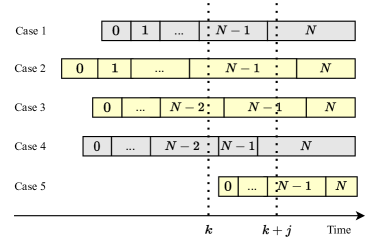
Using the information available at time $k$, the set $\mathcal{L}\left(k+j\mid k\right)$ of parcels that contribute to $L\left(k+j\right)$ is partitioned into several subsets. The set

$$\mathcal{L}_{N}\!\left(k+j\mid k\!\right) =\!\left\{\tau\mid T_{N-1}\!\left(\tau\!\right)\leqslant k,T_{N}\!\left(\tau\!\right)>k+j\!\right\}$$

contains the indexes of parcels known to be delivered (Status $N-1$) to the considered PUP before time $k$ and expected to be still waiting to be picked-up at time $k+j$. The set

$$\mathcal{L}_{n}\left(k+j\mid k\right) =\left\{\tau\mid T_{n-1}\left(\tau\right)\leqslant k,T_{n}\left(\tau\right)>k,T_{N-1}\left(\tau\right)\leqslant k+j,T_{N}\left(\tau\right)>k+j\right\}$$

contains the indexes of parcels with known status $n-1$ before time $k$, with $0<n<N$, for which $T_{n}\left(\tau\right)>k$ is unknown at time $k$, and which are expected to be delivered to the PUP before time $k+j$ and to be still waiting to be picked-up at time $k+j$. Finally, the set

$$\mathcal{L}_{0}\!\left(k+j\mid k\!\right)\!=\!\left\{\tau\mid T_{0}\!\left(\tau\!\right)\!>k,T_{N-1}\!\left(\tau\!\right)\!\leqslant k+j,T_{N}\!\left(\tau\!\right)\!>k+j\!\right\}$$

contains the indexes of parcels containing products not yet ordered at time $k$, but which are expected to be waiting to be picked-up in the target PUP $\rho$ at time $k+j$. Again, these parcels need to be delivered before time $k+j$.

Consequently,

$$\mathcal{L}\left(k+j\mid k\right)=\bigcup_{n=0}^{N}\mathcal{L}_{n}\left(k+j\mid k\right).$$ (5)

Figure 2 illustrates parcels with different status at time $k$ and the evolution of their status with time. Only a subset of these parcels contributes to the load of the PUP $\rho$ at time $k+j$.

4.2 Contribution to the load for each set of parcels

Let $\Lambda_{\tau}\left(k\right)$ be the random variable describing the contribution of each parcel $\tau$ to the load of the PUP $\rho$ at time $k$, i.e., $\Lambda_{\tau}\left(k\right)=1$ if the parcel waits to be picked-up at time $k$ and $\Lambda_{\tau}\left(k\right)=0$ else. Let $\mathcal{P}_{k}^{\rho}$ be the set of parcels with target PUP $\rho$ for which information is available at time $k$. Consequently

$$L\left(k\right)=\textstyle\sum_{\tau\in\mathcal{P}_{k}^{\rho}}\Lambda_{\tau}\left(k\right).$$ (6)

At time $k$, to evaluate the predicted load $L\left(k+j\mid k\right)$ at time $k+j$, one considers the partition of parcels introduced in (5) to get

$$L\left(k+j\mid k\right)={\textstyle\sum_{n=0}^{N}L_{n}\left(k+j\mid k\right),}$$ (7)

where $L_{n}\left(k+j\mid k\right)$ is the cardinal number of the set $\mathcal{L}_{n}\left(k+j\mid k\right)$. The random variables $L_{n}\left(k+j\mid k\right)$ are assumed to be independent. Consequently, the pmf of $L\left(k+j\mid k\right)$ is obtained as the convolution of the pmfs of all $L_{n}\left(k+j\mid k\right)$, $n=0,\dots,N$.

In this section, considering the status of a parcel $\tau$ at time $k$, one evaluates its probability to belong to $\mathcal{L}\left(k+j\mid k\right)$, i.e., to contribute to the load of the considered PUP at time $k+j$.

Proposition 1

At time $k$, consider a parcel $\tau$ with current status $S_{k}=N-1$, i.e., that has been delivered at time $t_{N-1}\leqslant k$ and that has not yet been picked up time $k$. The pickup time $T_{N}$ depends on the delivery time $T_{N-1}$, and implicitly on the opening hours of the PUP $\rho$. The probability that $\tau\in\mathcal{L}_{N}\left(k+j\mid k\right)$, i.e., that it is still in the PUP at time $k+j$, $j\geqslant 1$ is

$$\mathbb{P}\left(\Lambda_{\tau}\left(k+j\right)=1\mid T_{N-1}=t_{N-1},T_{N}>k\right) =\mathbb{P}\left(T_{N}>k+j\mid T_{N-1}=t_{N-1},T_{N}>k\right)$$

$$=\frac{1-\sum_{t_{N}=t_{N-1}+1}^{k+j}f_{N-1}\left(t_{N}-t_{N-1}\mid t_{N-1}\right)}{1-\sum_{t_{N}=t_{N-1}+1}^{k}f_{N-1}\left(t_{N}-t_{N-1}\mid t_{N-1}\right)}.$$ (8)

The proof of Proposition 1 is provided in Appendix A.1.

Proposition 2

At time $k$, consider a parcel $\tau$ with current status $S_{k}=N-2$ and carrier $C\left(\tau\right)=c$. This parcel is still in transit to the target PUP at time $k$. The delivery time $T_{N-1}$ depends on the carrier $c$ and on the time $T_{N-2}$ (of collection, e.g., at the dispatch center closest to the PUP). The probability that $\tau\in\mathcal{L}_{N-1}\left(k+j\mid k\right)$, i.e., that it is delivered before time $k+j$ and still in the PUP at time $k+j$, $j\geqslant 1$ is

$\displaystyle\mathbb{P}$ $\displaystyle\left(\Lambda_{\tau}\left(k+j\right)=1\mid T_{N-2}=t_{N-2},T_{N-1}>k,c\right)=\mathbb{P}\!\left(T_{N-1}\!\leqslant k+j,T_{N}\!>k+j|T_{N-2}\!=t_{N-2},T_{N-1}\!>k,c\right),$ $\displaystyle=\frac{\displaystyle\sum_{t_{N-1}=k+1}^{k+j}f_{N-2}\left(t_{N-1}-t_{N-2}\mid t_{N-2}\right)}{1-\displaystyle\sum_{t_{N-1}=t_{N-2}+1}^{k}f_{N-2}\left(t_{N-1}-t_{N-2}\mid t_{N-2}\right)}\cdot\left(1-\frac{\displaystyle\sum_{t_{N-1}=k+1}^{k+j-1}\sum_{t_{N}=t_{N-1}+1}^{k+j}f_{N-1}\left(t_{N}-t_{N-1}\mid t_{N-1}\right)f_{N-2}\left(t_{N-1}-t_{N-2}\mid t_{N-2}\right)}{\displaystyle\sum_{t_{N-1}=k+1}^{k+j}f_{N-2}\left(t_{N-1}-t_{N-2}\mid t_{N-2}\right)}\right).$ (9)

The proof of Proposition 1 is provided in Appendix A.2. In (9), the dependency in $c$ of $f_{N-2}$ has been omitted.

Proposition 3

At time $k$, consider a parcel $\tau$ with current status $S_{k}=n$, $0<n<N-2$, reached at time $t_{n}$. The parcel is shipped by carrier $C\left(\tau\right)=c$ to the target PUP $\rho$. The probability that $\tau\in\mathcal{L}_{n+1}\left(k+j\mid k\right)$, i.e., that it is delivered before time $k+j$ and still in the PUP at time $k+j$, $j\geqslant 1$ is

$\displaystyle\mathbb{P}$ $\displaystyle\left(\Lambda_{\tau}\left(k+j\right)=1\mid T_{n}=t_{n},T_{n+1}>k,r,c\right)=\mathbb{P}\!\left(T_{N-1}\!\leqslant k+j,T_{N}\!>k+j\!\mid T_{n}=t_{n},T_{n+1}\!>k,r,c\right)$ $\displaystyle=\frac{\sum_{t_{N-1}=k+1}^{k+j}g_{n}^{N-1}\left(t_{n},t_{N-1}\right)}{1-\sum_{t_{n+1}=t_{n}+1}^{k}f_{n}\left(t_{n+1}-t_{n}\mid t_{n}\right)}\cdot\left(1-\frac{\displaystyle\sum_{t_{N}=k+1}^{k+j}\displaystyle\sum_{t_{N-1}=k+1}^{t_{N}}\sum_{t_{n+1}=k+1}^{t_{N-1}}f_{N-1}\left(t_{N}-t_{N-1}\mid t_{N-1}\right)g_{n+1}^{N-1}\left(t_{n+1},t_{N-1}\right)f_{n}\left(t_{n+1}-t_{n}\mid t_{n}\right)}{\displaystyle\sum_{t_{N-1}=k+1}^{k+j}\sum_{t_{n+1}=k+1}^{t_{N-1}}g_{n+1}^{N-1}\left(t_{n+1},t_{N-1}\right)f_{n}\left(t_{n+1}-t_{n}\mid t_{n}\right)}\right),$ (10)

The function

$$g_{n}^{N-1}\left(t_{n},t_{N-1}\right) =\sum_{t_{n+1}=k+1}^{t_{N-1}}\sum_{t_{n+2}=t_{n+1}+1}^{t_{N-1}}\dots\sum_{t_{N-2}=t_{N-3}+1}^{t_{N-1}}f_{N-2}\left(t_{N-1}-t_{N-2}\mid t_{N-2}\right)\dots$$

$$f_{n+1}\left(t_{n+2}-t_{n+1}\mid t_{n+1}\right)f_{n}\left(t_{n+1}-t_{n}\mid t_{n}\right).$$ (11)

in (11) represents the probability for a parcel to switch from status $n$ reached at time $t_{n}$ to status $N-1$ at time $t_{N-1}$.

The proof of Proposition 3 is provided in Appendix A.3.

In (10) and (11), the dependency of $f_{n}$ with the carrier $c$ has been omitted. Moreover, in (11), all sums have been written with up to $t_{N-1}$ to lighten notations. Nevertheless, as there is at least one time interval $T$ between consecutive transitions, one has $f_{n+1}\left(0\mid t_{n+1},c\right)=0$, and many terms in (11) will vanish.

Proposition 4

At time $k$, consider a parcel $\tau$ that will be ordered at time $T_{0}\left(\tau\right)=t_{0}$ with $k<t_{0}<k+j$ with target PUP $\rho$. The parcel preparation duration $H_{0}\left(\tau\right)=T_{1}\left(\tau\right)-T_{0}\left(\tau\right)$ depends on the retailer $r$, and the delivery time depends on the carrier $c$. The probability that $\tau\in\mathcal{L}_{\text{0}}\left(k+j\mid k\right)$, i.e., that it is delivered before time $k+j$ and still in the PUP at time $k+j$, $j\geqslant 1$ is

$\displaystyle\mathbb{P}$ $\displaystyle\left(\Lambda_{\tau}\left(k+j\right)=1\mid T_{0}=t_{0},r,c\right)=\mathbb{P}\left(T_{N-1}\leqslant k+j,T_{N}>k+j\mid T_{0}=t_{0},r,c\right)$ $\displaystyle=\sum_{t_{N-1}=k+1}^{k+j}\sum_{t_{0}=k+1}^{t_{N-1}}g_{0}^{N-1}\left(t_{0},t_{N-1}\right)\cdot\left(1-\frac{\displaystyle\sum_{t_{0}=k+1}^{k+j-\left(N-1\right)}\sum_{t_{N-1}=t_{0}+N-1}^{k+j-1}\sum_{t_{N}=t_{N-1}+1}^{k+j}f_{N-1}\left(t_{N}-t_{N-1}\mid t_{N-1}\right)g_{0}^{N-1}\left(t_{0},t_{N-1}\right)}{\displaystyle\sum_{t_{0}=k+1}^{k+j-\left(N-1\right)}\sum_{t_{N-1}=t_{0}+N-1}^{k+j}g_{0}^{N-1}\left(t_{0},t_{N-1}\right)}\right).$ (12)

The proof of Proposition 4 can be found in Appendix A.4. In (12), the dependency of (12) in $r$ and $c$ has also been omitted.

The number of parcels that may contribute to $\mathcal{L}_{\text{0}}\left(k+j\mid k\right)$ is not known at time $k$, contrary to parcels that may contribute to $\mathcal{L}_{n}\left(k+j\mid k\right)$, $0<n\leqslant N-1$ for which more information is available (their order is at least confirmed). To address this issue, we choose to model the number of orders $O\left(k+i\mid k\right)$ that will be confirmed at time $k+i$ with a generalized Poisson model [24] with parameter $\lambda_{\text{O}}\left(k+i\mid k\right)$.

Introducing $L_{\text{0},k+i}\left(k+j\mid k\right)$, the random variable representing the number of parcels contributing to the load at time $k+j$ among those to be ordered in the time slot $k+i$, $i=1,\dots,j$, one may write the random variable describing the parcels ordered after the time interval $k$ as

$$L_{0}\left(k+j\mid k\right)=L_{\text{0},k+1}\left(k+j\mid k\right)+\dots+L_{\text{0},k+j}\left(k+j\mid k\right).$$ (13)

One has

$$\mathbb{P}\left(L_{\text{0},k+i}\left(k+j\mid k\right)=\ell\right)=\sum_{m=0}^{\infty}\mathbb{P}\left(L_{\text{0},k+i}\left(k+j\mid k\right)=\ell\mid O\left(k+i\mid k\right)=m\right)\cdot\mathbb{P}\left(O\left(k+i\mid k\right)=m\right).$$ (14)

The pmf $\mathbb{P}\left(L_{\text{0},k+i}\left(k+j\mid k\right)=\ell\mid O\left(k+i\mid k\right)=m\right)$ is then evaluated as

$$\mathbb{P}\left(L_{\text{0},k+i}\left(k+j\mid k\right)=\ell\mid O\left(k+i\mid k\right)=m\right)=\mathbb{P}\left({\textstyle\sum_{\tau\in\mathbb{V}_{k+i,m}}\Lambda_{\tau}\left(k+j\right)=\ell}\right),$$ (15)

where $\mathbb{V}_{k+i,m}$ is the set of virtual parcel indexes (since not known at time $k$), with $\left|\mathbb{V}_{k+i,m}\right|=m$, and such that for all $\tau\in\mathbb{V}_{k+i,m}$, $T_{0}\left(\tau\right)=k+i$. Assuming again that the random variables $\Lambda_{\tau}\left(k+j\right)$, $\tau\in\mathbb{V}_{k+i,m}$ are independent, the pmf of $\sum_{\tau\in\mathbb{V}_{k+i,m}^{r}}\Lambda_{\tau}\left(k+j\right)$ is obtained as the convolutions of the $m$ pmfs of $\Lambda_{\tau}\left(k+j\right)$ when $\tau\in\mathbb{V}_{k+i,m}$, which is evaluated using Proposition 4. Note that for all $\tau\in\mathbb{V}_{k+i,m}$, $r$ and $c$ are unknown, as the parcel has not been ordered at time $k$. One may choose $r$ and $c$ at random according to estimated retailer and carrier selection probabilities $\mathbb{P}\left(R=r\right)$ and $\mathbb{P}\left(C=c\mid R=r\right)$, as the carrier may depend on the retailer.

4.3 Load prediction algorithm

Algorithm 1 summarizes the evaluation of the probability mass function of the load $p_{L,k+j\mid k}$ for time $k+j$ using knowledge available up to time $k$. From Line 2 to 7, the contribution to the load of each parcel in $\mathcal{P}_{k}^{\rho}$, i.e., which status is known at time $k$ is evaluated. The load_contrib function provides the pmf of $\Lambda_{\tau}(k+j)$ using Proposition 1, 2, or 3, depending on the current known status $n$ of the parcel $\tau$. From Line 8 to 18, the contribution of parcels that will be ordered after time $k$ is evaluated. Each possible future order time instant $k+i$ is considered. Then, at Line 10, the pmf $\Lambda_{\tau}(k+i)$ is evaluated using Proposition 4. Only $m_{\max}$ terms in the sum (14) are considered. This requires a prediction of the expected number $\lambda_{\text{O}}(k+i\mid k)$ of future orders at Line 11. Then (15) and (14) are evaluated iteratively at Line 16 and 17. Finally, at Line 18, the contribution of future orders is integrated in that of parcels which status is known at time $k$.

The functions load_contrib and future_load_contrib invole the transition probability functions (3). The way they may be estimated as well as the evaluation of $\lambda_{\text{O}}(k+i\mid k)$ is detailed in Section 5.

Input : $k$; $j$; $\mathcal{P}_{k}^{\rho}$; $\lambda_{\text{O}}$;

Output : $p_{L,k+j\mid k}$

1

2begin

       // Init. pmf of $L(k+j\mid k)$

3      

4      $p_{L,k+j\mid k}\longleftarrow[1,0,\dots,0]$

5      foreach $\tau\in\mathcal{P}_{k}^{\rho}$ do

6            

            // Eval. contrib. of $\tau$ to $L(k+j\mid k)$

7            

            $n\longleftarrow S_{k}\left(\tau\right)$ // Current status

8            

            $t_{n}\longleftarrow T_{n}\left(\tau\right)$ // Entering time

9            

            // Eval. $p_{\tau}$ pmf of $\Lambda_{\tau}(k+j)$ using Props 1-3 depending on $n$

10             $p_{\tau}\longleftarrow\textnormal{{load\_contrib}}(n,t_{n},k,j)$

            // Update pmf of $L(k+j\mid k)$

11             $p_{L,k+j\mid k}\longleftarrow\textnormal{{convolve}}(p_{L,k+j\mid k},p_{\tau})$

      // Init. pmf $p_{\text{F}}$ of $L_{0}(k+j\mid k)$ (contrib. of future orders)

12      

13      $p_{\text{F}}\longleftarrow[1,0,\dots,0]$

      // Loop on future order times $k+i$

14       foreach $i\in[1,j-1]$ do

             // Eval $p_{\tau}$ pmf of $\Lambda_{\tau}(k+i)$ see Prop. 4

15            

16            $p_{\tau}\longleftarrow\textnormal{{future\_load\_contrib}}(i,k)$

            /* Eval. $\lambda_{\text{O}}(k+i\mid k)$ for Poisson model for nb of orders at time $k+i$ */

17             $\lambda\longleftarrow\textnormal{{eval\_lambda(i,k)}}$

            /* $m_{max}$ s.t. Poisson cdf with param. $\lambda(k+i\mid k)$ is larger than 0.99 */

18             $m_{\text{max}}\longleftarrow\textnormal{{ppf\_poisson}}(\lambda(k+i\mid k),0.99)$

            /* Init. pmf of $L_{\text{0},k+i}\left(k+j\mid k\right)$ knowing that $O\left(k+i\mid k\right)$ */

19             $p_{0}\longleftarrow[1,0,\dots,0]$

            // Init. pmf of $L_{\text{0},k+i}\left(k+j\mid k\right)$

20             $q_{i}\longleftarrow[1,0,\dots,0]$

            // For each nb $m$ of orders

21            

22            foreach $m\in[1,m_{\max}]$ do

23                  

                  // Iter. eval. of (15) using $p_{m}$

24                  

25                  $p_{m}\longleftarrow\textnormal{{convolve}}(p_{m-1},p_{\tau})$

                  // Iter. eval. of (14) using $q_{i}$

26                   $q_{i}\longleftarrow q_{i}+p_{m}\cdot\frac{e^{-\lambda}\lambda^{m}}{m!}$

27            $p_{\text{F}}\longleftarrow\textnormal{{convolve}}(p_{\text{F}},q_{i})$

28      

      // Update $p_{L,k+j\mid k}$ with contrib. of orders after time $k$

29       $p_{L,k+j\mid k}\longleftarrow\textnormal{{convolve}}(p_{L,k+j\mid k},p_{\text{F}})$

30      return $p_{L,k+j\mid k}$ 

31

Algorithm 1 Load prediction algorithm

5 Application

Figure 3 shows the typical life-cycle of a parcel $\tau$ containing a product purchased by a customer from an online retailer at time $t_{0}$ and chosen to be delivered at a PUP $\rho$. The order is processed by the retailer and is ready for expedition at time $t_{\text{1}}.$ Carrier $C\left(\tau\right)\in\Gamma$ takes the parcel over from the retailer warehouse at time $t_{\text{2}}$ and delivers it to the chosen PUP at time $t_{\text{3}}$. The delay between $t_{\text{2}}$ and $t_{\text{3}}$ depends on $C\left(\tau\right)$ and on the relative location of the warehouse and of the PUP. Processing at intermediate dispatch centers are integrated in the delay between $t_{2}$and $t_{3}$. In most of the cases, the parcel is accepted by the PUP and waits until it is picked up by the customer at time $t_{\text{4}}$. The parcel is returned to the retailer warehouse when its maximum sojourn time is reached. Some parcels may be refused by the PUP in case of overload or closure and are rerouted to an alternative PUP. This possibility is not considered in what follows.

Figure 3: Life-cycle of a parcel

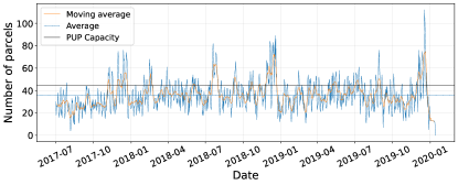
To illustrate the proposed PUP load prediction approach, we consider a local shop serving as PUP in Roussillon (France). Figure 4 shows the evolution of its load at 13:00 from July 2017 to December 2019. The PUP has a capacity of $45$ parcels and is open from 9:00 to 19:00, from Monday to Saturday and from 9:00 to 12:00 on Sundays. Sunday is not a working day for carriers in that area. This PUP has had no long closing periods from 2017 to 2019. The data used to obtain the load evolution are available in the database.

Figure 4: Evolution of the load at 13:00 of the considered PUP from July 2017 to December 2019.

5.1 Model

In the considered database, the time of order validation is not available. Moreover, only the day at which parcels are ready to be delivered is available. Consequently, in the life cycle of a parcel introduced in Section 5, only three statuses are considered, namely taken over ($S\left(\tau\right)=2$), delivered ($S\left(\tau\right)=3$), and picked-up ($S\left(\tau\right)=4$). The picked-up status is also associated to returned parcels, since the effect of picked-up and returned parcels on the PUP load is the same. Moreover, there are three possible carriers $\Gamma=\left\{1,2,3\right\}$.

For a parcel $\tau$ with status $S\left(\tau\right)=2$, the delay between taken-over and delivery to the PUP $H_{2}\left(\tau\right)=T_{3}\left(\tau\right)-T_{2}\left(\tau\right)$ depends on the carrier $C=c$ (as the delivery delay differs among carriers), and on the day of the week $w\left(T_{2}\left(\tau\right)\right)$ the parcel has been taken over, i.e.,

$$\mathbb{P}\left(H_{3}=t_{3}-t_{2}\mid T_{2}=t_{2},C=c\right)=f_{2}\left(t_{3}-t_{2}\mid w\left(t_{2}\right),c\right).$$

The delay between delivery and pick-up $H_{3}\left(\tau\right)=T_{4}\left(\tau\right)-T_{3}\left(\tau\right)$ depends on the day of the week and on the hour of delivery. Consequently, the distribution of $H_{3}$ knowing $T_{3}=t_{3}$ is such that

$$\mathbb{P}\left(H_{3}=t_{4}-t_{3}\mid T_{3}=t_{3}\right) =f_{3}\left(t_{4}-t_{3}\mid w\left(t_{3}\right),h\left(t_{3}\right)\right),$$ (16)

i.e., only the day of the week and the hour of $t_{3}$ are accounted for in the variability of the pmf $f_{3}$ of $H_{3}\left(\tau\right)$.

5.2 Estimation of the pmf $f_{n}$

In this paper, empirical frequencies are evaluated to obtain the components of the pmf $f_{n}$. Alternatively, parametric models could have been considered.

As $f_{2}$ only depends on the day of the week $w$ a parcel has been taken over and of the carrier $c$, the estimation of $f_{2}\left(\delta t\mid w,c\right)$ is performed considering $w=1,\dots,7$ and $c=1,2,3$. Consequently only $3\times 7$ different pmfs are estimated. For each of these pmfs, delivery delays ranging from $\delta t=0$ h to $\delta t=100$ h, are considered, since the delivery delay is generally within 5 days (day off included). There is a relatively important variability in the delivery hour among PUPs, only data related to parcels with the PUP $\rho$ as target are considered for the estimation of $f_{2}\left(\delta t\mid w,c\right)$. Assuming that the estimation is performed at time $k$, for given values of $w$ and $c$, one gets

$$\widehat{f}_{2}\left(\delta t\mid w,c\right)=\frac{\left|\left\{\tau\in\mathcal{P}_{k}^{\rho}\mid h_{2}\left(\tau\right)=\delta t,w\left(t_{2}\left(\tau\right)\right)=w,t_{3}\left(\tau\right)\leqslant k,C\left(\tau\right)=c\right\}\right|}{\left|\left\{\tau\in\mathcal{P}_{k}^{\rho}\mid w\left(t_{2}\left(\tau\right)\right)=w,C\left(\tau\right)=c,t_{3}\left(\tau\right)\leqslant k\right\}\right|},$$

where $\mathcal{P}_{k}^{\rho}$ is the set of parcels for which information is available at time $k$ with PUP $\rho$ as target, whatever their status. Moreover, $h_{2}\left(\tau\right)$, $t_{2}\left(\tau\right)$, and $t_{3}\left(\tau\right)$ are the observed value of $H_{2}\left(\tau\right)$, $T_{2}\left(\tau\right)$, and $T_{3}\left(\tau\right)$ for parcel $\tau$.

The pmf $f_{3}$ of the delay between parcel delivery and pick-up depends on the day of the week $w$ and hour $h$ of delivery. The estimation of $f_{3}\left(\delta t\mid w,h\right)$ is thus performed for $w=1,\dots,7$ and $h=h_{\text{o}}\left(w\right),\dots,h_{\text{c}}\left(w\right)$, where $h_{\text{o}}\left(w\right)$ and $h_{\text{c}}\left(w\right)$ are the opening and closing hours of the PUP $\rho$ for the week day $w$. For the PUP $\rho$, this represents about $76$ different pmfs to estimate, each with $\delta t=0,\dots,336$ h, to account for a maximum parcel sojourn time of two weeks in the PUP before being returned. Assuming again an estimation performed at time $k$, for a given value of $w$ and $h$, one gets

$$\widehat{f}_{3}\left(\delta t\mid w,h\right)=\frac{\left|\left\{\tau\in\mathcal{P}_{k}^{\rho}\mid h_{3}\left(\tau\right)=\delta t,w\left(t_{3}\left(\tau\right)\right)=w,h\left(t_{3}\left(\tau\right)\right)=h,t_{4}\left(\tau\right)\leqslant k\right\}\right|}{\left|\left\{\tau\in\mathcal{P}_{k}^{\rho}\mid w\left(t_{3}\left(\tau\right)\right)=w,h\left(t_{3}\left(\tau\right)\right)=h,t_{4}\left(\tau\right)\leqslant k\right\}\right|}$$

where $h_{3}\left(\tau\right)$, $t_{3}\left(\tau\right)$, and $t_{4}\left(\tau\right)$ are the observed value of $H_{3}\left(\tau\right)$, $T_{3}\left(\tau\right)$, and $T_{4}\left(\tau\right)$ for parcel $\tau$.

The pmfs $f_{n}$, $n=2,3$ account well for regular closing days, e.g., on Sundays via the conditioning on the weekday $w$. Nevertheless, on days off (New Year, First of May), there may be no parcel collection or delivery. When the PUP is closed on days off and for holidays, there are no parcel delivery and pick up too. PUP closing days are usually known in advance by the PMC. The impact of known closing days may be easily taken into account to update the estimates of $f_{n}$.

5.3 Prediction of the number of parcel orders

In the considered context, no information is available about parcel orders. Consequently, instead of trying to estimate the number of parcel that will be ordered at time $k+j$, one estimates the number of parcels that will be taken over at time $k+i$, $i=1,\dots,j$ and which may contribute to the load of the PUP at time $k+j$.

Let $O\left(k\mid c\right)=\text{Card}\left(\left\{\tau\,|\,T_{0}\left(\tau\right)=k,C\left(\tau\right)=c\right\}\right)$ be a random variable describing the number of parcels taken over at time $k$ by Carrier $c$ and to be delivered to the PUP $\rho$. The sequence $\left\{O\left(k\mid r\right)\right\}$ is a count time series, described by a generalized Poisson model with time-varying parameter $\lambda_{\text{O}}\left(k,c\right)$.

Considering the hourly breakdown of parcels taken over by Carrier $c$ (with PUP $\rho$ as target) during a day, one has

$$\lambda_{\text{O}}\left(k,r\right)=\rho_{w\left(k\right)}^{c}\left(h\left(k\right)\right)\mu_{c}\left(k-h\left(k\right)\right),$$ (17)

where $\rho_{w}^{c}\left(h\right)\geqslant 0$ is the proportion of parcels taken over by Carrier $c$ during the time interval $\left[hT,\left(h+1\right)T\right[$ of the week day $w$ and is such that $\sum_{h}\rho_{w}\left(h\right)=1$, $w=1,\dots,7$. Moreover, $\mu_{c}\left(k-h\left(k\right)\right)$ is the number of parcels taken over by Carrier $c$ during the whole day starting at time $\left(k-h\left(k\right)\right)T$.

Using information available at time $k$, the parameters $\rho_{w}^{c}\left(h\right)$ are estimated as

$$\widehat{\rho}_{w}^{c}\left(h\right) =\frac{\left|\left\{\tau\in\mathcal{P}_{k}^{\rho}\mid w\!\left(T_{1}\!\left(\tau\!\right)\!\right)=w,h\!\left(T_{1}\!\left(\tau\!\right)\!\right)=h,C\!\left(\tau\!\right)=c\!\right\}\right|}{\left|\left\{\tau\in\mathcal{P}_{k}\mid w\!\left(T_{1}\!\left(\tau\!\right)\!\right)=w,C\!\left(\tau\!\right)=c\!\right\}\right|},$$ (18)

where $\mathcal{P}_{k}^{\rho}$ is the set of parcels for which information is available at time $k$, whatever their status and their target PUP. The sequence $\left\{\mu_{r}\right\}$ is a non-negative count time series, for which we consider a SARIMA model [25] to estimate future values.

6 Results

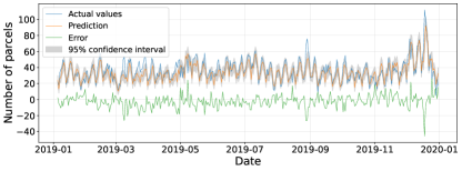
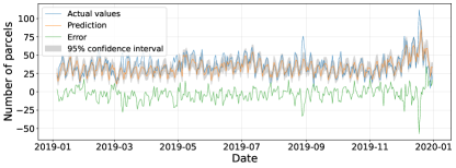
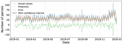
Table 2 shows the prediction error of $L\left(k+j\mid k\right)$ considering a prediction performed at midnight of each day. The obtained results are compared with the direct prediction of the load at 13:00 of each day considered as a time series described by a Holt-Winters [26] model, a SARIMA model, a SARIMAX model with the prediction of the number of delivered parcels as exogenous variable, a Random Forest [27] model, several LSTM [28] models, and our previously parcel flow-based approach [7].

An MAE of 4.47 parcels is obtained for $j=13$ (one-day ahead prediction) and of $8.12$ parcels for $j=85$ (four-day ahead prediction). These results outperform the direct prediction using the other models, especially the SARIMAX model that integrates also prior knowledge on parcels already taken over by a carrier, as well as for our previously proposed parcel flow-based approach. This illustrates the benefits of taking into account the various parcels statuses during the delivery process.

Approach	$j=13$		$j=37$		$j=61$		$j=85$
	MAE	MAPE	MAE	MAPE	MAE	MAPE	MAE	MAPE
Holt-Winters	6.74	18.4	8.48	24.3	9.68	27.5	10.12	28.3
SARIMA	6.42	17.9	7.65	22.4	8.44	24.9	8.7	26.2
SARIMAX	5.33	14.40	7.03	20.30	7.99	23.60	8.45	25.1
Random Forest	6.85	20.3	8.67	26.9	9.28	30.2	9.44	30.8
Stacked-LSTM	9.30	26.4	11.49	38.1	12.31	36.5	12.94	39.3
Bi-LSTM	9.62	28.0	11.93	35.3	13.30	36.2	13.65	35.5
Conv-LSTM	8.20	23.2	10.37	32.7	11.16	36.6	11.03	41.5
Parcel flow [7]	5.65	14.1	7.77	19.8	9.31	24.1	10.17	26.8
Parcel life-cycle	4.47	12.9	6.06	18.4	7.21	21.2	8.12	23.7

Table 2: MAE and MAPE of the prediction errors of $L\left(k+j\mid k\right)$ for the proposed and alternative approaches.

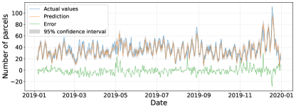
Figures 5 to 6 compare the actual and predicted values of the load $L\left(k+j\mid k\right)$ for $k=13,37,61,85$. For $j\geqslant 65$ (three and four day ahead prediction), there is an important prediction error before Christmas. The activity peak is not well predicted by the SARIMA model used in the proposed approach to predict future orders.

Figure 5: Predicted and actual value of $L\left(k+13\right)$ (top) and $L\left(k+37\right)$ (bottom) and prediction errors

Figure 6: Predicted and actual value of $L\left(k+61\right)$ (top) and $L\left(k+85\right)$ (bottom) and prediction errors

7 Conclusion

This paper introduces a load forecasting approach for PUPs, leveraging on a Markov jump process model of the life cycle of parcels. This approach has been applied to predict the load related to B2C e-commerce. The propose approach outperforms alternative techniques more agnostic of the parcel life-cycle, which consider the load as a time series.

Future work includes increasing the prediction horizon to 7 days ahead by gathering information on the number of future parcels to be processed from the carriers and the online retailers. A load-balancing method must be developed to distribute upcoming parcels among PUPs. The proposed models must also be adapted to forecast the load of automatic parcel lockers with more constraints due to the limited number of locker units for parcels of multiple sizes.

Appendix A Proofs

A.1 Proof of Proposition 1

At time $k$, consider a parcel $\tau$ with current status $S_{k}=N-1$, i.e., that has been delivered at time $t_{N-1}\leqslant k$, and that has not yet been picked up at time $k$. The probability that $\tau\in\mathcal{L}_{N}\left(k+j|k\right)$, i.e., that it is still in the PUP at time $k+j$, $j\geqslant 1$ is

$$\mathbb{P}\left(\Lambda_{\tau}\left(k+j\right)=1\mid T_{N-1}=t_{N-1},T_{N}>k\right)=\mathbb{P}\left(T_{N}>k+j\mid T_{N-1}=t_{N-1},T_{N}>k\right).$$ (19)

Then (19) is rewritten as

$$\mathbb{P}\left(T_{N}>k+j\mid T_{N-1}=t_{N-1},T_{N}>k\right) =\frac{\mathbb{P}\left(T_{N}>k+j,T_{N}>k\mid T_{N-1}=t_{N-1}\right)}{\mathbb{P}\left(T_{N}>k\mid T_{N-1}=t_{N-1}\right)}$$

$$=\frac{\mathbb{P}\left(T_{N}>k+j\mid T_{N-1}=t_{N-1}\right)}{\mathbb{P}\left(T_{N}>k\mid T_{N-1}=t_{N-1}\right)}$$

$$=\frac{1-\mathbb{P}\left(T_{N}\leqslant k+j\mid T_{N-1}=t_{N-1}\right)}{1-\mathbb{P}\left(T_{N}\leqslant k\mid T_{N-1}=t_{N-1}\right)}$$

$$=\frac{1-\sum_{t_{N}=t_{N-1}+1}^{k+j}f_{N-1}\left(t_{N}-t_{N-1}\mid t_{N-1}\right)}{1-\sum_{t_{N}=t_{N-1}+1}^{k}f_{N-1}\left(t_{N}-t_{N-1}\mid t_{N-1}\right)}$$

where $f_{N-1}\left(t_{N}-t_{N-1}\mid t_{N-1}\right)$ is given by (3).

A.2 Proof of Proposition 2

At time $k$, consider a parcel $\tau$ with current status $S_{k}=N-2$, i.e., that has reached a dispatch center at time $t_{N-2}\leqslant k$ and has not been delivered at time $k$. The probability that $\tau\in\mathcal{L}_{N-1}\left(k+j|k\right)$, i.e., that it is delivered before time $k+j$ and still in the PUP at time $k+j$, $j\geqslant 1$ is

$$\mathbb{P}\left(\Lambda_{\tau}\left(k+j\right)=1\mid T_{N-2}=t_{N-2},T_{N-1}>k\right) =\mathbb{P}\left(T_{N-1}\leqslant k+j,T_{N}>k+j\mid T_{N-2}=t_{N-2},T_{N-1}>k\right),$$ (20)

One may rewrite (20) as

$$\mathbb{P}\left(\Lambda_{\tau}\left(k+j\right)=1\mid T_{N-2}=t_{N-2},T_{N-1}>k\right) =\mathbb{P}\left(T_{N-1}\leqslant k+j\mid T_{N-2}=t_{N-2},T_{N-1}>k\right)$$

$$\mathbb{P}\left(T_{N}>k+j\mid k<T_{N-1}\leqslant k+j,T_{N-2}=t_{N-2}\right).$$ (21)

Consider the first term of (21),

$$\mathbb{P}\left(T_{N-1}\leqslant k+j\mid T_{N-2}=t_{N-2},T_{N-1}>k\right) =\frac{\mathbb{P}\left(T_{N-1}\leqslant k+j,T_{N-1}>k\mid T_{N-2}=t_{N-2}\right)}{\mathbb{P}\left(T_{N-1}>k\mid T_{N-2}=t_{N-2}\right)}$$

$$=\frac{\sum_{t_{N-1}=k+1}^{k+j}\mathbb{P}\left(T_{N-1}=t_{N-1}\mid T_{N-2}=t_{N-2}\right)}{1-\sum_{t_{N-1}=t_{N-2}+1}^{k}\mathbb{P}\left(T_{N-1}=t_{N-1}\mid T_{N-2}=t_{N-2}\right)}$$

$$=\frac{\sum_{t_{N-1}=k+1}^{k+j}f_{N-2}\left(t_{N-1}-t_{N-2}\mid t_{N-2}\right)}{1-\sum_{t_{N-1}=t_{N-2}+1}^{k}f_{N-2}\left(t_{N-1}-t_{N-2}\mid t_{N-2}\right)}.$$ (22)

The second term of (21) is

$$\mathbb{P}\left(T_{N}>k+j\mid k<T_{N-1}\leqslant k+j,T_{N-2}=t_{N-2}\right) =1-\mathbb{P}\left(T_{N}\leqslant k+j\mid k<T_{N-1}\leqslant k+j,T_{N-2}=t_{N-2}\right)$$

$$=1-\frac{\mathbb{P}\left(T_{N}\leqslant k+j,k<T_{N-1}\leqslant k+j\mid T_{N-2}=t_{N-2}\right)}{\mathbb{P}\left(k<T_{N-1}\leqslant k+j\mid T_{N-2}=t_{N-2}\right)}$$

$$=1-\frac{\sum_{t_{N-1}=k+1}^{k+j-1}\mathbb{P}\left(T_{N}\leqslant k+j,T_{N-1}=t_{N-1}\mid T_{N-2}=t_{N-2}\right)}{\sum_{t_{N-1}=k+1}^{k+j}\mathbb{P}\left(T_{N-1}=t_{N-1}\mid T_{N-2}=t_{N-2}\right)}.$$ (23)

In (23), one has

$$\mathbb{P}\left(T_{N}\leqslant k+j,T_{N-1}=t_{N-1}\mid T_{N-2}=t_{N-2}\right) =\mathbb{P}\left(T_{N}\leqslant k+j\mid T_{N-1}=t_{N-1},T_{N-2}=t_{N-2}\right)$$

$$\cdot\mathbb{P}\left(T_{N-1}=t_{N-1}\mid T_{N-2}=t_{N-2}\right)$$

$$=\mathbb{P}\left(T_{N}\leqslant k+j\mid T_{N-1}=t_{N-1}\right)$$

$$\cdot f_{N-2}\left(t_{N-1}-t_{N-2}\mid t_{N-2}\right).$$ (24)

using the Markov property and (3). Then

$$\mathbb{P}\left(T_{N}\leqslant k+j\mid T_{N-1}=t_{N-1}\right) =\sum_{t_{N}=k+1}^{k+j}\mathbb{P}\left(T_{N}=t_{N}\mid T_{N-1}=t_{N-1}\right)$$

$$=\sum_{t_{N}=k+1}^{k+j}f_{N-1}\left(t_{N}-t_{N-1}\mid t_{N-1}\right).$$ (25)

Finally, combining (21) to (25), one gets

$$\mathbb{P}\left(\Lambda_{\tau}\left(k+j\right)=1\mid T_{N-2}=t_{N-2},T_{N-1}>k\right) =\frac{\sum_{t_{N-1}=k+1}^{k+j}f_{N-2}\left(t_{N-1}-t_{N-2}\mid t_{N-2}\right)}{1-\sum_{t_{N-1}=t_{N-2}+1}^{k}f_{N-2}\left(t_{N-1}-t_{N-2}\mid t_{N-2}\right)}$$

$$\left(1-\frac{\sum_{t_{N-1}=k+1}^{k+j-1}\sum_{t_{N}=k+1}^{k+j}f_{N-1}\left(t_{N}-t_{N-1}\mid t_{N-1}\right)f_{N-2}\left(t_{N-1}-t_{N-2}\mid t_{N-2}\right)}{\sum_{t_{N-1}=k+1}^{k+j}f_{N-2}\left(t_{N-1}-t_{N-2}\mid t_{N-2}\right)}\right).$$ (26)

A.3 Proof of Proposition 3

At time $k$, consider a parcel $\tau$ with current status $S_{k}=n$, reached at time $t_{n}$, with $0<n<N-1$. This parcel is shipped by carrier $C\left(\tau\right)=c$ to the target PUP $\rho$. The probability that $\tau\in\mathcal{L}_{n}\left(k+j\mid k\right)$, i.e., that it is delivered before time $k+j$ and still in the PUP at time $k+j$, $j\geqslant 1$ is

$$\mathbb{P}\left(\Lambda_{\tau}\left(k+j\right)=1\mid T_{n}=t_{n},T_{n+1}>k\right) =\mathbb{P}\left(T_{N-1}\!\leqslant k+j,T_{N}\!>k+j\mid T_{n}=t_{n},T_{n+1}\!>k\right).$$ (27)

Using the conditional probability, (27) can be rewritten as

$$\mathbb{P}\left(\Lambda_{\tau}\left(k+j\right)=1\mid T_{n}=t_{n},T_{n+1}>k\right) =\mathbb{P}\left(T_{N-1}\leqslant k+j\mid T_{n}=t_{n},T_{n+1}>k\right)$$

$$\mathbb{P}\left(T_{N}>k+j\mid T_{n}=t_{n},T_{n+1}>k,T_{N-1}\leqslant k+j\right).$$ (28)

Consider the first term of (28),

$$\mathbb{P}\left(T_{N-1}\leqslant k+j\mid T_{n}=t_{n},T_{n+1}>k\right) =\frac{\mathbb{P}\left(T_{N-1}\leqslant k+j,T_{n+1}>k\mid T_{n}=t_{n}\right)}{\mathbb{P}\left(T_{n+1}>k\mid T_{n}=t_{n}\right)}$$

$$=\frac{\sum_{t_{N-1}=k+1}^{k+j}\sum_{t_{n+1}=k+1}^{t_{N-1}}\mathbb{P}\left(T_{N-1}=t_{N-1},T_{n+1}=t_{n+1}\mid T_{n}=t_{n}\right)}{1-\sum_{t_{n+1}=t_{n}+1}^{k}\mathbb{P}\left(T_{n+1}=t_{n+1}\mid T_{n}=t_{n}\right)}$$ (29)

In the denominator of (29), one has

$$\mathbb{P}\left(T_{n+1}=t_{n+1}\mid T_{n}=t_{n}\right)=\sum_{t_{n+1}=t_{n}+1}^{k}f_{n}\left(t_{n+1}-t_{n}\mid t_{n}\right)$$

For the numerator of (29), one has

$$\mathbb{P}\left(T_{N-1}=t_{N-1},T_{n+1}=t_{n+1}\mid T_{n}=t_{n}\right) =\mathbb{P}\left(T_{N-1}=t_{N-1}\mid T_{n+1}=t_{n+1},T_{n}=t_{n}\right)$$

$$\cdot\mathbb{P}\left(T_{n+1}=t_{n+1}\mid T_{n}=t_{n}\right)$$

$$=\mathbb{P}\left(T_{N-1}=t_{N-1}\mid T_{n+1}=t_{n+1}\right)$$

$$\cdot\mathbb{P}\left(T_{n+1}=t_{n+1}\mid T_{n}=t_{n}\right).$$

Then

$$\mathbb{P}\left(T_{N-1}=t_{N-1}\mid T_{n+1}=t_{n+1}\right) =\sum_{t_{n+2}=t_{n+1}+1}^{t_{N-1}}\mathbb{P}\left(T_{N-1}=t_{N-1},T_{n+2}=t_{n+2}\mid T_{n+1}=t_{n+1}\right)$$

$$=\sum_{t_{n+2}=t_{n+1}+1}^{t_{N-1}}\mathbb{P}\left(T_{N-1}=t_{N-1}\mid T_{n+2}=t_{n+2}\right)$$

$$\cdot\mathbb{P}\left(T_{n+2}=t_{n+2}\mid T_{n+1}=t_{n+1}\right).$$

This process may be iterated up to $\mathbb{P}\left(T_{N-1}=t_{N-1}\mid T_{N-2}=t_{N-2}\right)$ to get finally

$$\mathbb{P}\left(T_{N-1}\leqslant k+j,T_{n+1}>k\mid T_{n}=t_{n}\right) =\sum_{t_{N-1}=k+1}^{k+j}\sum_{t_{n+1}=k+1}^{t_{N-1}}\sum_{t_{n+2}=t_{n+1}+1}^{t_{N-1}}\dots\sum_{t_{N-2}=t_{N-3}+1}^{t_{N-1}}\mathbb{P}\left(T_{N-1}=t_{N-1}\mid T_{N-2}=t_{N-2}\right)\dots$$

$$\mathbb{P}\left(T_{n+2}=t_{n+2}\mid T_{n+1}=t_{n+1}\right)\mathbb{P}\left(T_{n+1}=t_{n+1}\mid T_{n}=t_{n}\right)$$

$$=\sum_{t_{N-1}=k+1}^{k+j}g_{n}^{N-1}\left(t_{n},t_{N-1}\right)$$

where

$$g_{n}^{N-1}\left(t_{n},t_{N-1}\right)= \sum_{t_{n+1}=k+1}^{t_{N-1}}\sum_{t_{n+2}=t_{n+1}+1}^{t_{N-1}}\dots\sum_{t_{N-2}=t_{N-3}+1}^{t_{N-1}}f_{N-2}\left(t_{N-1}-t_{N-2}\mid t_{N-2}\right)$$

$$\dots f_{n+1}\left(t_{n+2}-t_{n+1}\mid t_{n+1}\right)f_{n}\left(t_{n+1}-t_{n}\mid t_{n}\right)$$

which is the probability for a parcel to switch from status $n$ in which it is at time $t_{n}$ to status $N-1$ at time $t_{N-1}$. Consequently, the first term of (28) is

$$\mathbb{P}\left(T_{N-1}\leqslant k+j\mid T_{n}=t_{n},T_{n+1}>k\right) =\frac{\sum_{t_{N-1}=k+1}^{k+j}g_{n}^{N-1}\left(t_{n},t_{N-1}\right)}{1-\sum_{t_{n+1}=t_{n}+1}^{k}f_{n}\left(t_{n+1}-t_{n}\mid t_{n}\right)}.$$ (30)

Consider the second term of (28),

$$\mathbb{P}\left(T_{N}>k+j\mid T_{n}=t_{n},T_{n+1}>k,T_{N-1}\leqslant k+j\right) =1-\mathbb{P}\left(T_{N}\leqslant k+j\mid T_{n}=t_{n},T_{n+1}>k,T_{N-1}\leqslant k+j\right)$$

$$=1-\frac{\mathbb{P}\left(T_{N}\leqslant k+j,T_{N-1}\leqslant k+j,T_{n+1}>k\mid T_{n}=t_{n}\right)}{\mathbb{P}\left(T_{N-1}\leqslant k+j,T_{n+1}>k\mid T_{n}=t_{n}\right)}.$$ (31)

Consider the denominator of (31),

$$\mathbb{P}\left(T_{N-1}\leqslant k+j,T_{n+1}>k\mid T_{n}=t_{n}\right) =\sum_{t_{N-1}=k+1}^{k+j}\sum_{t_{n+1}=k+1}^{t_{N-1}}\mathbb{P}\left(T_{N-1}=t_{N-1},T_{n+1}=t_{n+1}\mid T_{n}=t_{n}\right)$$

$$=\sum_{t_{N-1}=k+1}^{k+j}\sum_{t_{n+1}=k+1}^{t_{N-1}}\sum_{t_{n+2}=t_{n+1}+1}^{t_{N-1}}\mathbb{P}\left(T_{N-1}=t_{N-1},T_{n+2}=t_{n+2},T_{n+1}=t_{n+1}\mid T_{n}=t_{n}\right)$$

$$=\sum_{t_{N-1}=k+1}^{k+j}\sum_{t_{n+1}=k+1}^{t_{N-1}}\sum_{t_{n+2}=t_{n+1}+1}^{t_{N-1}}\mathbb{P}\left(T_{N-1}=t_{N-1},T_{n+2}=t_{n+2}\mid T_{n+1}=t_{n+1}\right)$$

$$\mathbb{P}\left(T_{n+1}=t_{n+1}\mid T_{n}=t_{n}\right).$$

This process may again be iterated to get

$$\mathbb{P}\left(T_{N-1}\leqslant k+j,T_{n+1}>k\mid T_{n}=t_{n}\right) =\sum_{t_{N-1}=k+1}^{k+j}\sum_{t_{n+1}=k+1}^{t_{N-1}}g_{n+1}^{N-1}\left(t_{n+1},t_{N-1}\right)\mathbb{P}\left(T_{n+1}=t_{n+1}\mid T_{n}=t_{n}\right)$$

$$=\sum_{t_{N-1}=k+1}^{k+j}\sum_{t_{n+1}=k+1}^{t_{N-1}}g_{n+1}^{N-1}\left(t_{n+1},t_{N-1}\right)f_{n}\left(t_{n+1}-t_{n}\mid t_{n}\right).$$ (32)

Consider the numerator of (31)

$$\mathbb{P} \left(T_{N}\leqslant k+j,T_{N-1}\leqslant k+j,T_{n+1}>k\mid T_{n}=t_{n}\right)=$$

$$\sum_{t_{N}=k+1}^{k+j}\sum_{t_{N-1}=k+1}^{t_{N}}\sum_{t_{n+1}=k+1}^{t_{N-1}}\mathbb{P}\left(T_{N}=t_{N},T_{N-1}=t_{N-1},T_{n+1}=t_{n+1}\mid T_{n}=t_{n}\right)$$ (33)

Then

$$\mathbb{P}\left(T_{N}=t_{N},T_{N-1}=t_{N-1},T_{n+1}=t_{n+1}\mid T_{n}=t_{n}\right) =\mathbb{P}\left(T_{N}=t_{N}\mid T_{N-1}=t_{N-1},T_{n+1}=t_{n+1},T_{n}=t_{n}\right)$$

$$\cdot\mathbb{P}\left(T_{N-1}=t_{N-1},T_{n+1}=t_{n+1}\mid T_{n}=t_{n}\right)$$

$$=\mathbb{P}\left(T_{N}=t_{N}\mid T_{N-1}=t_{N-1}\right)$$

$$\cdot\mathbb{P}\left(T_{N-1}=t_{N-1},T_{n+1}=t_{n+1}\mid T_{n}=t_{n}\right)$$

$$=f_{N-1}\left(t_{N}-t_{N-1}\mid t_{N-1}\right)g_{n+1}^{N-1}\left(t_{n+1},t_{N-1}\right)f_{n}\left(t_{n+1}-t_{n}\mid t_{n}\right).$$

Then

$$\mathbb{P} \left(T_{N}\leqslant k+j,T_{N-1}\leqslant k+j,T_{n+1}>k\mid T_{n}=t_{n}\right)=$$

$$\sum_{t_{N}=k+1}^{k+j}\sum_{t_{N-1}=k+1}^{t_{N}}\sum_{t_{n+1}=k+1}^{t_{N-1}}f_{N-1}\left(t_{N}-t_{N-1}\mid t_{N-1}\right)g_{n+1}^{N-1}\left(t_{n+1},t_{N-1}\right)f_{n}\left(t_{n+1}-t_{n}\mid t_{n}\right)$$ (34)

Finally, combining (30), (32), and (34), one gets

$$\mathbb{P}\left(\Lambda_{\tau}\left(k+j\right)=1\mid T_{n}=t_{n},T_{n+1}>k\right)=\frac{\sum_{t_{N-1}=k+1}^{k+j}g_{n}^{N-1}\left(t_{n},t_{N-1}\right)}{1-\sum_{t_{n+1}=t_{n}+1}^{k}f_{n}\left(t_{n+1}-t_{n}\mid t_{n}\right)}$$

$$\cdot\left(1-\frac{\sum_{t_{N}=k+1}^{k+j}\sum_{t_{N-1}=k+1}^{t_{N}}\sum_{t_{n+1}=k+1}^{t_{N-1}}f_{N-1}\left(t_{N}-t_{N-1}\mid t_{N-1}\right)g_{n+1}^{N-1}\left(t_{n+1},t_{N-1}\right)f_{n}\left(t_{n+1}-t_{n}\mid t_{n}\right)}{\sum_{t_{N-1}=k+1}^{k+j}\sum_{t_{n+1}=k+1}^{t_{N-1}}g_{n+1}^{N-1}\left(t_{n+1},t_{N-1}\right)f_{n}\left(t_{n+1}-t_{n}\mid t_{n}\right)}\right).$$

A.4 Proof of Proposition 4

At time $k$, consider a parcel $\tau$ that is expected to be ordered at time $T_{0}\left(\tau\right)=t_{0}$ with $k<t_{0}<k+j$ with target PUP $\rho$. The parcel preparation duration $H_{0}\left(\tau\right)=T_{1}\left(\tau\right)-T_{0}\left(\tau\right)$ depends on the retailer $r$, and the delivery time depends on the carrier $c$. In the rest of the proof we omit explicit references to the carrier $c$ and the retailer $r$. The probability that $\tau\in\mathcal{L}_{\text{0}}\left(k+j\mid k\right)$, i.e., that it is delivered before time $k+j$ and still in the PUP at time $k+j$, $j\geqslant 1$ is

$$\mathbb{P}\left(L_{0}\left(k+j\right)=1\mid T_{0}=t_{0}\right) =\mathbb{P}\left(T_{N-1}\leqslant k+j,T_{N}>k+j\mid T_{0}=t_{0}\right).$$ (35)

Using the properties of conditional probability, (35) can be rewritten as

$$\mathbb{P}\left(L_{0}\left(k+j\right)=1\mid T_{0}=t_{0}\right) =\mathbb{P}\left(T_{N-1}\leqslant k+j\mid T_{0}=t_{0}\right)$$

$$\times\mathbb{P}\left(T_{N}>k+j\mid T_{0}=t_{0},T_{N-1}\leqslant k+j\right).$$ (36)

Consider the first factor of (36),

$$\mathbb{P}\left(T_{N-1}\leqslant k+j\mid T_{0}=t_{0}\right) =\sum_{t_{N-1}=k+1}^{k+j}\mathbb{P}\left(T_{N-1}=t_{N-1}\mid T_{0}=t_{0}\right)$$ (37)

Moreover one has

$$\mathbb{P}\left(T_{N-1}=t_{N-1}\mid T_{0}=t_{0}\right) =g_{0}^{N-1}\left(t_{0},t_{N-1}\right).$$

Consequently,

$$\mathbb{P}\left(T_{N-1}\leqslant k+j\mid T_{0}=t_{0}\right)=\sum_{t_{N-1}=k+1}^{k+j}g_{0}^{N-1}\left(t_{0},t_{N-1}\right).$$ (38)

Consider the second factor of (36),

$$\mathbb{P}\left(T_{N}>k+j\mid T_{0}=t_{0},T_{N-1}\leqslant k+j\right) =1-\mathbb{P}\left(T_{N}\leqslant k+j\mid T_{0}=t_{0},T_{N-1}\leqslant k+j\right)$$

$$=1-\frac{\mathbb{P}\left(T_{N}\leqslant k+j,T_{N-1}\leqslant k+j\mid T_{0}=t_{0}\right)}{\mathbb{P}\left(T_{N-1}\leqslant k+j\mid T_{0}=t_{0}\right)}.$$ (39)

The denominator of (39) simplifies

$$\mathbb{P}\left(T_{N-1}\leqslant k+j\mid T=t_{0}\right) =\sum_{t_{N-1}=t_{0}+N-1}^{k+j}\mathbb{P}\left(T_{N-1}=t_{N-1}\mid T_{0}=t_{0}\right)$$

$$=\sum_{t_{N-1}=t_{0}+N-1}^{k+j}g_{0}^{N-1}\left(t_{0},t_{N-1}\right).$$ (40)

Consider the numerator of (39)

$$\mathbb{P}\left(T_{N}\leqslant k+j,T_{N-1}\leqslant k+j\mid T_{0}=t_{0}\right)=\sum_{t_{N-1}=t_{0}+N-1}^{k+j-1}\sum_{t_{N}=t_{N-1}+1}^{k+j}\mathbb{P}\left(T_{N}=t_{N},T_{N-1}=t_{N-1}\mid T_{0}=t_{0}\right),$$ (41)

in which each term of the double sum evaluates to

$$\mathbb{P}\left(T_{N}=t_{N},T_{N-1}=t_{N-1}\mid T_{0}=t_{0}\right) =\mathbb{P}\left(T_{N}=t_{N}\mid T_{N-1}=t_{N-1},T_{0}=t_{0}\right)\mathbb{P}\left(T_{N-1}=t_{N-1}\mid T_{0}=t_{0}\right)$$

$$=\mathbb{P}\left(T_{N}=t_{N}\mid T_{N-1}=t_{N-1}\right)\mathbb{P}\left(T_{N-1}=t_{N-1}\mid T_{0}=t_{0}\right)$$

$$=f_{N-1}\left(t_{N}-t_{N-1}\mid t_{N-1}\right)g_{0}^{N-1}\left(t_{0},t_{N-1}\right).$$ (42)

Finally, combining (36), (40), (41), and (42), one gets

$$\mathbb{P}\left(\Lambda_{\tau}\left(k+j\right)=1\mid T_{0}=t_{0}\right)= \sum_{t_{N-1}=k+1}^{k+j}g_{0}^{N-1}\left(t_{0},t_{N-1}\right)$$

$$\cdot\left(1-\frac{\sum_{t_{N-1}=t_{0}+N-1}^{k+j-1}\sum_{t_{N}=t_{N-1}+1}^{k+j}f_{N-1}\left(t_{N}-t_{N-1}\mid t_{N-1}\right)g_{0}^{N-1}\left(t_{0},t_{N-1}\right)}{\sum_{t_{N-1}=t_{0}+N-1}^{k+j}g_{0}^{N-1}\left(t_{0},t_{N-1}\right)}\right).$$

References

- [1] RSF. B2C E-commerce Market Size, Share & Trends Analysis Report by Type (B2C Retailers, Classifieds), by Application (Home Decor & Electronics, Clothing & Footwear), by Region and Segment Forecasts, 2020 - 2027. Technical report, ResearchAndMarkets.com, 2020.
- [2] L. K. de Oliveira, E. Morganti, L. Dablanc, and R. L. M. de Oliveira, ‘Analysis of the potential demand of automated delivery stations for e-commerce deliveries in Belo Horizonte, Brazil’, Research in Transportation Economics, vol. 65, pp. 34–43, 2017.
- [3] E. Morganti, L. Dablanc, and F. Fortin, ‘Final deliveries for online shopping: The deployment of pickup point networks in urban and suburban areas’, Research in Transportation Business & Management, vol. 11, pp. 23–31, 2014.
- [4] J. W. J. Weltevreden, ‘B2c e-commerce logistics: the rise of collection-and-delivery points in The Netherlands’, International Journal of Retail & Distribution Management, vol. 36, no. 8, pp. 638–660, Jan. 2008.
- [5] S. Iwan, K. Kijewska, and J. Lemke, ‘Analysis of Parcel Lockers’ Efficiency as the Last Mile Delivery Solution – The Results of the Research in Poland’, Transportation Research Procedia, vol. 12, pp. 644–655, 2016.
- [6] M. Zhou, L. Zhao, N. Kong, K. S. Campy, G. Xu, G. Zhu, X. Cao, and S. Wang, ‘Understanding consumers’ behavior to adopt self-service parcel services for last-mile delivery’, Journal of Retailing and Consumer Services, vol. 52, p. 101911, 2020.
- [7] T.-T.-T. Nguyen, A. Cabani, I. Cabani, K. De Turck, and M. Kieffer, ‘Load prediction of parcel pick-up points: model-driven vs data-driven approaches’, International Journal of Production Research, pp. 1–30., 2023.
- [8] I. Cardenas, Y. Borbon-Galvez, T. Verlinden, E. Van de Voorde, T. Vanelslander, and W. Dewulf, ‘City logistics, urban goods distribution and last mile delivery and collection’, Competition and Regulation in Network Industries, vol. 18, no. 1–2, pp. 22–43, Mar. 2017.
- [9] I. Cardenas, Y. Borbon-Galvez, T. Verlinden, E. Van de Voorde, T. Vanelslander, and W. Dewulf, ‘City logistics, urban goods distribution and last mile delivery and collection’, Competition and Regulation in Network Industries, vol. 12, no. 21, 2020.
- [10] J. Allen, M. Piecyk, M. Piotrowska, F. McLeod, T. Cherrett, K. Ghali, T. Nguyen, T. Bektas, O. Bates, A. Friday, S. Wise, and M. Austwick, CUnderstanding the impact of e-commerce on last-mile light goods vehicle activity in urban areas: The case of London’, Transportation Research Part D: Transport and Environment, vol. 61, pp. 325–338, 2018.
- [11] Y. Wang, Y. Zhang, M. Bi, J. Lai, and Y. Chen, ‘A Robust Optimization Method for Location Selection of Parcel Lockers under Uncertain Demands’, Mathematics, vol. 10, no. 22, 2022.
- [12] R. Gevaers, E. Voorde, and T. Vanelslander, ‘Characteristics of innovations in last mile logistics using best practices, case studies and making the link with green and sustainable logistics’, Proc. European Transport Conference, 2009.
- [13] H. Abbasimehr, M. Shabani, and M. Yousefi, ‘An optimized model using LSTM network for demand forecasting’, Computers & Industrial Engineering, vol. 143, p. 106435, 2020.
- [14] B. Zhang, M.-L. Tseng, L. Qi, Y. Guo, and C.-H. Wang, ‘A comparative online sales forecasting analysis: Data mining techniques’, Computers & Industrial Engineering, vol. 176, p. 108935, 2023.
- [15] H. Kurata and J. J. Liu, ‘Optimal promotion planning—depth and frequency—for a two-stage supply chain under Markov switching demand’, European Journal of Operational Research, vol. 177, no. 2, pp. 1026–1043, 2007.
- [16] S. J. Taylor and B. Letham., ‘Forecasting at scale’, PeerJ Preprints, 2017.
- [17] N. Cristianini and J. Shawe-Taylor, An Introduction to Support Vector Machines and Other Kernel-based Learning Methods. Cambridge University Press, 2000.
- [18] L. Guo, W. Fang, Q. Zhao, and X. Wang, ‘The hybrid PROPHET-SVR approach for forecasting product time series demand with seasonality’, Computers & Industrial Engineering, vol. 161, p. 107598, 2021.
- [19] N. Salari, S. Liu, Z.-J. M. Shen, ‘Real-Time Delivery Time Forecasting and Promising in Online Retailing: When Will Your Package Arrive?’, Manufacturing & Service Operations Management, vol. 24, no. 3, pp. 1421-1436, 2022.
- [20] Parcelmonitor. Dwell Time Analysis of Parcels in Collection Points. Technical report, 2021.
- [21] D. Brajon, C. Ropital, C. Delaporte, C. Tarquis, and F. Awada., ‘Comment ameliorer la performance logistique du e-commerce ?’, Technical report, Institut Paris Region, 2016.
- [22] W. J. Stewart, ‘Elementary Queueing Theory’, in Probability, Markov Chains, Queues, and Simulation, Princeton University Press, pp. 385–443, 2009.
- [23] P.-C. G. Vassiliou, ‘Non-Homogeneous Markov Set Systems’, Mathematics, vol. 9, no. 5, 2021.
- [24] C. W. S. Chen and S. Lee, ‘Generalized Poisson autoregressive models for time series of counts’, Computational Statistics & Data Analysis, vol. 99, pp. 51–67, 2016.
- [25] G. A. N. Pongdatu and Y. H. Putra, ‘Seasonal Time Series Forecasting using SARIMA and Holt Winter’s Exponential Smoothing’, IOP Conference Series: Materials Science and Engineering, vol. 407, no. 1, p. 012153, Aug. 2018.
- [26] C. C. Holt, ‘Forecasting seasonals and trends by exponentially weighted moving averages’, International Journal of Forecasting, vol. 20, no. 1, pp. 5–10, 2004.
- [27] L. Breiman, ‘Random Forests’, Machine Learning, vol. 45, no. 1, pp. 5–32, 2001.
- [28] B. Lakshmanan, P. S. N. Vivek Raja, and V. Kalathiappan, ‘Sales Demand Forecasting Using LSTM Network’, in Artificial Intelligence and Evolutionary Computations in Engineering Systems, pp. 125–132, 2020.