PDE-CNNs: Axiomatic Derivations and Applications

Abstract

PDE-based Group Convolutional Neural Networks (PDE-G-CNNs) utilize solvers of geometrically meaningful evolution PDEs as substitutes for the conventional components in G-CNNs. PDE-G-CNNs offer several key benefits all at once: fewer parameters, inherent equivariance, better performance, data efficiency, and geometric interpretability.
In this article we focus on Euclidean equivariant PDE-G-CNNs where the feature maps are two dimensional throughout. We call this variant of the framework a PDE-CNN.
We list several practically desirable axioms and derive from these which PDEs should be used in a PDE-CNN. Here our approach to geometric learning via PDEs is inspired by the axioms of classical linear and morphological scale-space theory, which we generalize by introducing semifield-valued signals.
Furthermore, we experimentally confirm for small networks that PDE-CNNs offer fewer parameters, better performance, and data efficiency in comparison to CNNs. We also investigate what effect the use of different semifields has on the performance of the models.

1 Introduction

1.1 Background

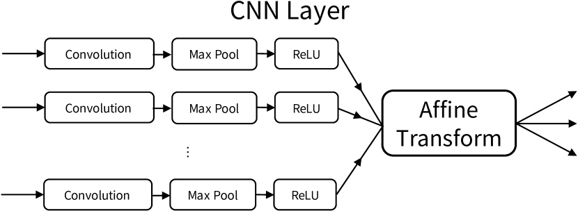
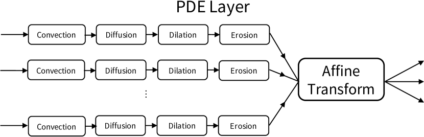
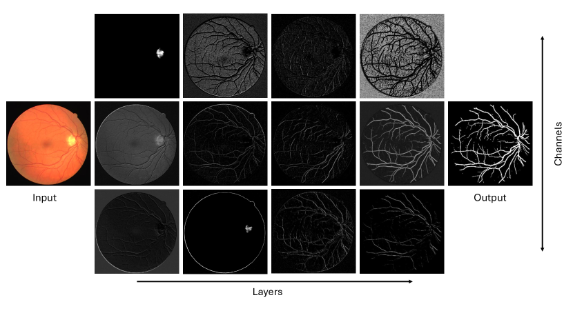
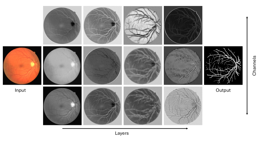
Recently, PDE-based group equivariant convolution neural networks (PDE-G-CNNs) [1] were introduced. PDE-G-CNNs belong to the broad family of group equivariant convolution neural works (G-CNNs) [2]. Unlike traditional CNNs, PDE based networks replace the usual components that make up a CNN layer, that being convolutions, max pooling, and non-linear activation functions, by solvers of evolution PDEs. The coefficients that govern the effect of the PDEs serve as the trainable parameters. Figure 1 contains a diagram of an example CNN layer and PDE layer, intended to illustrate the similarities and differences between them. Figure 2 visualizes some of the feature maps from trained networks that utilize either standard CNN layers or PDE layers.

(a) CNN layer.

(b) PDE layer

Figure 1: Diagram of an example CNN layer and PDE layer.

(a) Feature maps of a CNN.

(b) Feature maps of a PDE-CNN.

Figure 2: Illustration of (some of) the feature maps of a standard CNN and a PDE-CNN (both with 6 layers and 16 channels) trained to perform vessel segmentation of images of the fundus of the eye. Not all channels and layers are visualized; a representative selection was chosen.

It is shown in [3, 1, 4, 5] that PDE-G-CNNs have inherent equivariance, fewer parameters, increased performance, data efficiency, and better geometric interpretability, when compared to G-CNNs and classical CNNs. There is also a relation between PDE-G-CNNs and association fields [6] from neurogeometry [7, 8], further clarified in [4].

The PDE-G-CNN architecture is very general in the sense that the signals can be defined on any Lie group $G$ equipped with a left-invariant metric tensor field. However, the existing PDE-G-CNN literature [3, 1, 4, 5] mainly concerns itself with $G=\text{SE}(2)$, the group of two-dimensional rotations and translations. We will not consider the general setting, or $G=\text{SE}(2)$ for that matter, and restrict ourselves to $G=\mathbb{R}^{2}$, i.e. standard two-dimensional Euclidean space, for simplicity. We call this specific instance a PDE-CNN. In practice, working with PDE-CNNs, in comparison to the $\text{SE}(2)$ PDE-G-CNN, has the advantage of consuming less memory, and the disadvantage that only translation equivariance is included and not rotation equivariance.

In [1] the PDEs that are used in the PDE-G-CNN architecture are convection, diffusion, dilation, and erosion. These PDEs respectively correspond to shifting, blurring, max pooling, and min pooling. The first question that immediately arises is: why were these particular PDEs selected? The quick answer is that these PDEs come directly from the world of scale-space theory. This is what makes PDE-G-CNNs more geometrically meaningful and interpretable than traditional networks. To appreciate this answer we need to provide the appropriate background by introducing the concept of scale-space representations.

Real world scenes contain many different objects at different scales. When a computer is tasked with analyzing an image of a scene there is no way for it to know beforehand at which scale(s) the interesting structures live. One way to tackle this problem is to analyze the image of interest at all scales.

In broad terms, a scale-space representation of an image is an ordered collection of images where each successive image contains less and less detail; that is the smaller scales have been processed away. The collection of images is usually indexed by the scale-parameter $t\geq 0$ with $t=0$ being the original image. In the abstract ideal the scale parameter $t$ is continuous and the scale-space ranges all the way from scale $t=0$ to scales that are arbitrary large. In practice a discrete set of scales $t$ is chosen, usually in a exponential manner such as $t=1,4,16,64,256$ [9].

The prototypical, and most likely first [10, 11, 12], example of a scale-space is the Gaussian scale-space made by successive diffusing (i.e. blurring or smoothing) of the original image. The Gaussian scale-space $f_{t}$ of a two-dimensional image $f_{0}:\mathbb{R}^{2}\to\mathbb{R}$ can be written as a linear convolution $*$ with a Gaussian kernel $k_{t}$:

$$\begin{split}&f_{t}=k_{t}*f_{0},\quad k_{t}(x)=\frac{1}{2\pi t}\exp\left(-\frac{\|x\|^{2}}{2t}\right),\\ &(k_{t}*f_{0})(x)=\int_{\mathbb{R}^{2}}k_{t}(x-y)f_{0}(y){\rm d}y.\end{split}$$ (1)

Two other examples are the quadratic morphological scale-space representations [13] made by successively dilating or eroding the original image. The quadratic dilation scale-space can be written as a non-linear dilating convolution $\boxplus$ with a quadratic kernel:

$$\begin{split}&f_{t}=k_{t}\boxplus f_{0},\quad k_{t}(x)=-\frac{\|x\|^{2}}{2t},\\ &(k_{t}\boxplus f_{0})(x)=\sup_{y\in\mathbb{R}^{2}}k_{t}(x-y)+f_{0}(y).\end{split}$$ (2)

The quadratic erosion scale-space is created using a eroding convolution $\boxminus$:

$$\begin{split}&f_{t}=k_{t}\boxminus f_{0},\quad k_{t}(x)=\frac{\|x\|^{2}}{2t},\\ &(k_{t}\boxminus f_{0})(x)=\inf_{y\in\mathbb{R}^{2}}k_{t}(x-y)+f_{0}(y).\end{split}$$ (3)

The dilating and eroding convolutions are collected under the umbrella term morphological convolution. This is because they are related by the identity $-(-f\boxplus-g)=f\boxminus g$. The dilating and eroding convolutions can be seen as continuous versions of the max and min-pooling that is commonly used in CNNs.

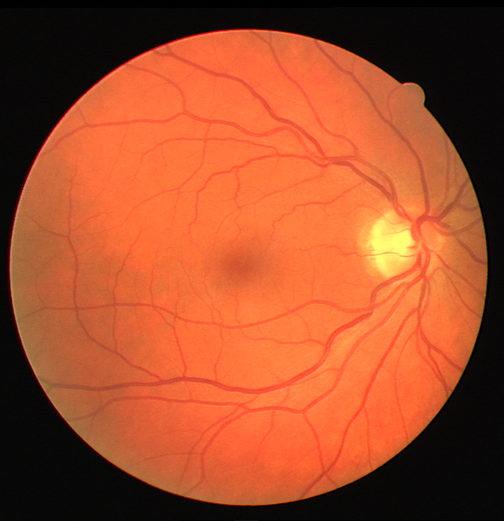
In Figure 3 the Gaussian, quadratic dilation, and quadratic erosion scale-spaces representations are visualized of a grayscale image of the fundus of the eye [14].

Figure 3: The Gaussian, quadratic dilation, and quadratic erosion scale-space representations of a grayscale image of the fundus of the eye at various scale-parameters. In the Gaussian scale-space both white and black features fade away towards a uniform image. In the dilation scale-space the black details (low values), such as the vessels, vanish at bigger scales. In the erosion scale-space the white details (high values), such as the space between vessels, are removed at higher scales.

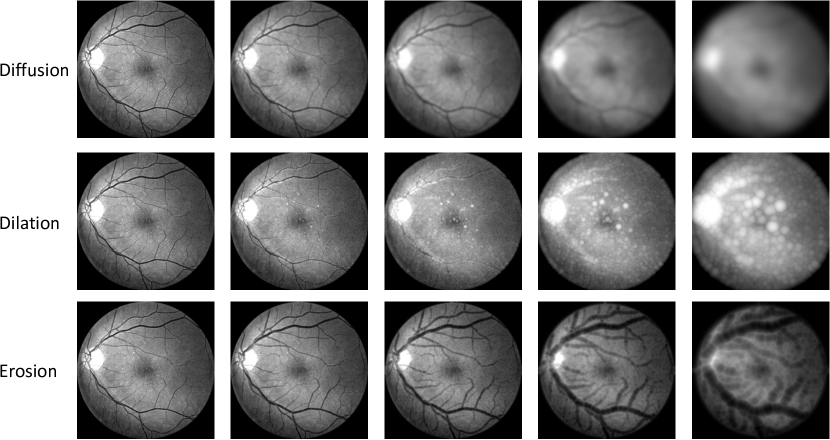
The Gaussian, quadratic dilation, and quadratic erosion scale-space representations can also be concisely described as the solution to an evolution PDE, with the input image being the initial condition. Namely, the Gaussian scale-space corresponds to the diffusion PDE $\frac{\partial f}{\partial t}=\frac{1}{2}\Delta f$, where $\Delta$ is the Laplacian, the quadratic dilation scale-space is the (viscosity) solution of dilation PDE $\frac{\partial f}{\partial t}=\frac{1}{2}\|\nabla f\|^{2}$, and the quadratic erosion corresponds to the erosion PDE $\frac{\partial f}{\partial t}=-\frac{1}{2}\|\nabla f\|^{2}$. We say the PDE generates the scale-space. It is PDEs such as these that PDE-G-CNNs employ.

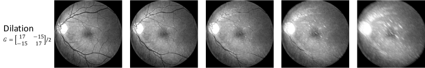
In the first paragraph of the introduction it was said that in a PDE-CNN the trainable parameters are the coefficients that determine the effect of the used PDEs. However, the PDEs we have seen just now have no free coefficients, so what is there to train? The explanation is that we do not solely utilize the standard inner product on $\mathbb{R}^{2}$; rather, we consider general inner products $\left\langle x,y\right\rangle_{G}=x^{T}Gy$, with $G\in\mathbb{R}^{2\times 2}$ a symmetric positive definite matrix. When using different inner products, concepts such as Laplacian, gradient, and norm change accordingly, consequently altering the effect of the PDEs that depend on them. In concrete terms, this means that in the formulas (1), (2), and (3) the norm $\|x\|$ is changed to $\|x\|_{G}:=\sqrt{x^{T}Gx}$. It is this matrix $G$ that is learned during training in the PDE-CNN framework. In Figure 4 the quadratic dilation scale-space representation is visualized with a non-standard inner product.

Figure 4: The quadratic dilation scale-space representation with the (very) anisotropic inner product $G=[[17,-15],[-15,17]]/2$. This can be compared with the dilation scale-space seen in Figure 3 that uses the standard isotropic inner product $G=I$. Such an anisotropic dilation can, for example, be used to remove unaligned vessels. This is best seen in the fourth image where only the diagonally oriented vessels are still apparent.

Scale-spaces are a natural choice for computer vision solutions(either neural networks or classical methods) as they respect the inherent symmetries of images, that being translation, rotational, and scaling symmetries. What we mean by this mathematically is that, for example, the scale-space $g_{t}$ of a translated image $g_{0}=T_{v}f_{0}$, is equal to the translated scale-space of the original image: $g_{t}=T_{v}f_{t}$. Here $T_{v}$ is the translation operator defined by $(T_{v}f)(x)=f(x-v)$. Analogous statements hold for the rotation and scaling symmetries. We say that creating the scale-space representation of an image is equivariant with respect to translation, rotations and scalings.

Scale-spaces respect the inherent symmetries of images, and this property transfers to neural networks that employ scale-spaces. That means that these architectures are inherently translation, rotation, and scaling equivariant. Architectures that are inherently equivariant enjoy benefits such as data efficiency, reduced parameter count, and robustness [16, 17]. From the translation equivariance (and a form of linearity) it also follows that the architectures that employ scale-spaces are naturally convolution neural networks, which are easy to implement and fast to evaluate due to the highly parallelizable nature of convolutional operations. In recent scale equivariant networks literature [18, 19, 20, 21] the link to scale-space theory is also emphasized. In fact, the architectures they design are scale-spaces in the broad sense.

To return to the question of why the diffusion, dilation, and erosion PDEs are employed in a PDE-G-CNNs, the answer is that these PDEs generate scale-spaces, and scale-spaces are a natural choice for computer vision solutions. However, this raises a follow-up question: are there any other PDEs that generate scale-spaces? To even start answering this question we need a proper mathematical definition of a scale-space, and this begins by explaining what we mean when we say a scale-space is (quasi)linear.

Creating Gaussian scale-spaces is linear in the sense that if one takes two images $f_{0},g_{0}:\mathbb{R}^{2}\to\mathbb{R}$ and two scalars $a,b\in\mathbb{R}$, then the scale-space $h_{t}$ of the image $h_{0}=af_{0}+bg_{0}$ is equal to $h_{t}=af_{t}+bg_{t}$. But, in an analogous manner, the quadratic dilation scale-space is quasilinear in the sense that the scale-space of the image $h_{0}=\max\{a+f_{0},b+g_{0}\}$, where we interpret the maximum pointwise, is equal to $h_{t}=\max\{a+f_{t},b+g_{t}\}$. In the same way, the quadratic erosion scale-space is quasilinear in the $\min$ sense. One can quickly check these properties through their convolutional form as seen above. To define what we mean with quasilinear more generally we need to introduce the notion of a semifield.

A semifield $(R,\mathbb{0},\mathbb{1},\oplus,\otimes)$ is an algebraic structure like a field but where we relax the requirement that the addition $\oplus$ has inverses. The prototypical example of a semifield are the nonnegative real numbers $L_{\geq 0}=(\mathbb{R}_{\geq 0},0,1,+,\times)$ with standard addition and multiplication. We have already seen two other examples of semifields in the dilating and eroding convolutions above. Namely, the tropical semifields ${T_{\scalebox{0.6}{$+$}}}=(\mathbb{R}\cup\{-\infty\},-\infty,0,\max,+)$ and ${T_{\scalebox{0.6}{$-$}}}=(\mathbb{R}\cup\{\infty\},\infty,0,\min,+)$. In the tropical semifields the minimum(or maximum) of two numbers becomes semifield addition, and normal addition becomes semifield multiplication (which can be confusing).

With the definition of a semifield we can state the quasilinearity of a scale-space formally as semifield $R$-linearity. So, like before, consider a semifield $R$ and two semifield-valued images $f_{0},g_{0}:\mathbb{R}^{2}\to R$ and two elements $a,b\in R$. Then by a scale-space being $R$-linear we mean that the scale-space of the $R$-linear combination of images $h_{0}=(a\otimes f_{0})\oplus(b\otimes g_{0})$ is equal to $R$-linear combination of scale-spaces $h_{t}=(a\otimes f_{t})\oplus(b\otimes g_{t})$. In other words, the operation that takes an image and returns its scale-space representation is a semifield linear operator. For example, the Gaussian scale-space is $L_{\geq 0}$-linear, the quadratic dilation scale-space is ${T_{\scalebox{0.6}{$+$}}}$-linear, and the quadratic erosion scale-space is ${T_{\scalebox{0.6}{$-$}}}$-linear.

It is argued in multiple works [12, 22, 23] in an axiomatic way that the only linear scale-space representations correspond to solutions of the fractional diffusion (pseudo-)PDE system on $\mathbb{R}^{2}\times\mathbb{R}_{\geq 0}$:

$$\begin{array}[]{lll}\frac{\partial f}{\partial t}&=-\frac{1}{\alpha}(-\Delta)^{\alpha/2}f,&t\geq 0\\ f(\cdot,0)&=f_{0},\end{array}$$ (4)

where $-(-\Delta)^{\alpha/2}$ is a (fractional) power of the Laplacian, and $\alpha>0$. In an completely analogous manner, one can show [24, 25] that the only morphological scale-spaces, that being scale-spaces that are ${T_{\scalebox{0.6}{$+$}}}$ or ${T_{\scalebox{0.6}{$-$}}}$ linear, correspond to (viscosity) solutions of the $\alpha$-dilation and $\alpha$-erosion PDE:

$$\begin{array}[]{lll}\frac{\partial f}{\partial t}&=\pm\frac{1}{\alpha}\|\nabla f\|^{\alpha},&t\geq 0\\ f(\cdot,0)&=f_{0},\end{array}$$ (5)

with $\alpha>1$.

The scale-space representations that these $\alpha$ dependent PDEs generate can also written in terms of linear, dilating, and eroding convolutions, just as the special quadratic ($\alpha=2$) cases as seen above in (1), (2) and (3). However, the kernels $k_{t}$ in these cases are slightly more involved.

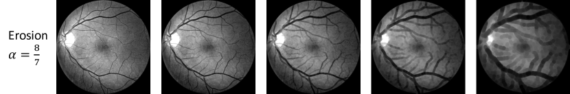
To give an example, the $\alpha$-erosion scale-space representation is given by

$$\begin{split}f_{t}=k_{t}\boxminus f_{0},\quad k_{t}(x)=\frac{t}{\beta}\left(\frac{\|x\|}{t}\right)^{\beta},\end{split}$$

with $1/\alpha+1/\beta=1$, and in Figure 5 the $\alpha=8/7$ case is visualized. The $\alpha>1$ parameter in this case regulates between “hard” min-pooling when $\alpha$ is close to 1, and “softer” min-pooling when $\alpha$ is bigger. In Figure 6 the kernel $k_{t}$ is visualized for different values of $\alpha$.

Figure 5: The $\alpha$-erosion scale-space representation with $\alpha=8/7$. This can be compared with the quadratic ($\alpha=2$) erosion scale-space seen in Figure 3. Notice that with smaller $\alpha$ the effect of the erosion becomes more abrupt and bokeh-like.

Figure 6: The shape of the $\alpha$-erosion scale-space kernel $k_{t}(x)=t(\|x\|/t)^{\beta}/\beta$ with $t=1$ and various values of $\alpha$.

Now, to return to the question of whether there are any other PDEs that generate scale-spaces. One answer to the question is that, other than the $\alpha$ dependent PDEs (4) and (5), there exist no other PDEs that generate linear or morphological scale-spaces. This answer is unsatisfactory of course, as it does not consider the possibility of using semifields other than linear and tropical ones.

1.2 Contributions

We take the standard scale-space axioms but state them in terms of semifields. This results in a definition that encapsulates a large class of known scale-spaces.

We will only consider semifields that are commutative and one-dimensional, and the scale-spaces their domain will be the two-dimensional Euclidean space $\mathbb{R}^{2}$. To maintain a practical perspective, we will consistently connect the overarching theory using five example semifields: the linear, root, logarithmic, tropical min, and tropical max semifields.

From the axioms we show in Theorem 1 that every semifield scale-space corresponds to a unique (one-parameter) family of scale-spaces, this being the main theoretical result of the article.

These theoretical results show that PDE-G-CNNs, in their current form, can be extended greatly by adding scale-spaces that correspond to various currently unutilized semifields.

We experimentally assess how effective the incorporation of new semifields and their corresponding scale-spaces is in Section 6.3, and verify that PDE-CNNs are simultaneously more data-efficient, have lower parameter count, and have competitive performance when compared to traditional CNNs in Section 6.2.

1.3 Short Outline

In Section 2 we provide a non-exhaustive list of related literature. In Section 3 we define semifields and all related structures and operations. This is necessary to define the semifield scale-space axioms. In Section 4 we state the semifield scale-space axioms. In Section 5 we show that once a semifield is chosen a unique (one-parameter) family of scale-spaces arise. This main result is Theorem 1. In Section 6 we briefly note on the architectural design of PDE-CNNs in practice, and we lay out two experiments and discuss their results. In Section 7 we conclude the article.

2 Related Work

In this section we provide a noncomprehensive list of related scale-space literature in chronological order.

• In T. Iijima’s paper [10] the first [11] axiomatic treatment of linear scale-space theory is presented. Axioms such as linearity, translation and rotation equivariance, one-parameter semigroup property, and most notably, the scale equivariance, can all be found in Iijima’s article.

• R. Brockett and P. Maragos [13] were the first [26] to show that morphological operators like dilations and erosions in image processing can be described in terms of nonlinear Hamilton–Jacobi PDEs, whose Lax-Oleinik solutions [15] boil down to quasi-linear convolutions over the tropical semifield (even on Riemannian homogeneous spaces [27, 28]). For PDE-based neural networks this allows for equivariant max-pooling over Riemannian balls (making RelU-activations obsolete) [1]

• In L. Alvarez, F. Guichard, P.L. Lions, and J.M. Morel [29] provide a very general axiomatic approach to PDE-based scale-spaces. The strength for geometric image processing of this approach is that it also includes mean curvatures flows [30] as highly powerful non-linear PDEs (also on Lie groups [31, 1]). Solutions of such non-linear PDEs may be solved with median filtering [32], however, they lack semifield linearity (taking mean/median are not associative binary operations). This makes those PDEs unfortunately less tangible for PDE-based neural networks where a form of linearity is important, both theoretically [3] and from a parallel GPU-implementation point of view. We will not insist in using solely (local) differential operators in our evolution generators, and more importantly, we take semifield linearity as a (restrictive) axiom.

• In E. Pauwels, L. van Gool, P. Fiddelaers, and T. Moons [22] an extended class of linear scale-spaces is introduced. They basically see that (fractional) powers of the Laplacian are valid linear scale-space generators, but never state the actual (pseudo-)PDE. Nevertheless, their work elegantly points out the restrictiveness of the scale-space axioms, with in particular the restrictive time scale equivariance axiom. Analysis of the scale-space axioms in the Fourier domain is extensively used, an approach that we also use in this article in the more general semifield setting. In the linear semifield setting we will end up with the same $\alpha$-stable Lévy processes (from the generalized CLT in probability theory [33]) as Pauwels et al. did, but also in other semifields (tropical, logarithmic, root) analysis via the corresponding semifield Fourier transform the technique by Pauwels works out well (as we will show).

• In L. Dorst and R. van den Boomgaard [34] the slope transform is presented. The slope transform is shown to be the morphological counterpart of the Fourier transform, and related to the Legendre-Fenchel transform. In fact, the Legendre-Fenchel transform can already be seen as the morphological equivalent of the Fourier transform if one restricts to convex/concave functions. The semifield Fourier transform we introduce reduces to the Legendre-Fenchel transform in the tropical semifield cases.

• In L. Florack [35] nonlinear scale-spaces are obtained by performing a monotonic transformation (known as a “Cole-Hopf” transform [15, Ch.4.4]) on the grey-values of a standard linear scale-space and deducing what nonlinear PDE corresponds to the obtained evolution. This transformation neatly bridges linear, logarithmic, and in the extreme cases, morphological scale-spaces, and we will use this link extensively.

• In H. J. Heijmans and R. van den Boomgaard [26] a very general algebraic framework for scale-spaces is given. Importantly, their perspective is (initially) totally divorced from PDEs, convolutions, and kernels, and focuses solely on the operator family. We will define our semifield scale-spaces in the same manner: The word ‘PDE’ is not present in our axioms, the PDEs solely come from algebraic symmetry constraints.

• In M. Welk [24] “Generalised morphological scale-spaces” are explored which look a lot like semifield scale-spaces. $\varphi$-deformed addition is defined by pulling back the standard linear semifield structure using the mapping $\varphi$. Linear, logarithmic, root, and tropical semifields all make an appearance, together with there corresponding semifield integration and scale-spaces. In this article we will rely on those useful scale-space tools and provide a general axiomatic derivation via the semifield Fourier transform.

• In M. Felsberg and G. Sommer [36] the Poisson scale-space is introduced, a linear scale-space that only fails to meet Koenderink’s principle. They introduce a weaker form of the causality axiom, which they call relaxed causality, and show that the Poisson scale-space does satisfy this relaxed notion. The Poisson scale-space fits within the scale-spaces of Pauwels et al. [22]. A key aspect of the Poisson scale-space is that it allows for a 3D Clifford analytic extension useful for phase based image processing [36]. This work will remain in the scalar-valued setting (and not study flow-field extensions) but we do include Poisson scale-space as a valid member, as it arises by the operator factorisation: $\Delta+\partial_{t}^{2}=(\partial_{t}-\sqrt{-\Delta})(\partial_{t}+\sqrt{-\Delta})$.

• In R. Duits, L. Florack, J. de Graaf, and B. ter Haar Romenij [37] the usual linear scale-space axioms together with extra axioms/properties such as weak/strong causality, increase of entropy and In the end the same conclusion as Pauwels et al. [22] is reached: fractional powers of the Laplacian $-(-\Delta)^{\alpha/2}$ generate valid scale-spaces and this is a special case of Yosida’s theory [38, ch:11] on strongly continuous semigroups. The $\alpha$-scale-spaces include Poisson ($\alpha=1$) and Gaussian ($\alpha=2$) scale-space, and coincides with the linear semifield scale-spaces we will axiomatically find in this article.

• In B. Burgeth and J. Weickert [39] the important connection between linear and morphological scale-spaces is illuminated using the Cramer transform. The Cramer transform gives us a way to translate between the kernels of the linear and morphological scale-spaces. We will show that all scale-spaces their kernel in a Fourier domain have the same form (this being our main theorem), illuminating further why this isomorphism from the linear to the tropical semifield makes sense. This transform is also used in [40] relating probability calculus on the linear semifield, to decision calculus on the tropical semifield.

• In M. Schmidt and J. Weickert [25] morphological counterparts of linear scale-spaces are explored. The Cramér–Fourier transform is introduced. This work directly builds on the previous work of B. Burgeth and J. Weickert [39], and is a modification of the Cramer transform. The Cramer-Fourier transform, in contrast to the Cramer transform, allows for a generalization to groups other than $\mathbb{R}^{2}$.

3 Semifield Theory

In this section we define semifields and all mathematical structures and operations made from them. This includes important concepts such as semimodules (Definition 7), linearity (Definition 8), measures (Definition 16), integration (Definition 18), integral operators (Definition 21), and Fourier transforms (Definition 26).

3.1 Semifield & Semimodules

Definition 1 (Semifield).

An commutative semifield $R$ is a tuple $R=(R,\mathbb{0},\mathbb{1},\oplus,\otimes)$ where $\oplus,\otimes:R\times R\to R$ are two commutative and associative binary operation on $R$ called semifield addition and multiplication, such that for all $a,b,c\in R$:

• $a\oplus\mathbb{0}=a$,

• $a\otimes\mathbb{1}=a$,

• $a\neq\mathbb{0}:\exists a^{-1}:a\otimes a^{-1}=\mathbb{1}$,

• $a\otimes\mathbb{0}=\mathbb{0}$,

• $a\otimes(b\oplus c)=(a\otimes b)\oplus(a\otimes b)$.

In other words, a semifield is a field where we do not require to have ”negative elements”, that being additive inverses. For simplicity we only consider commutative semifields in this article and drop the commutative adjective For brevity’s sake.

Throughout the article we will denote an arbitrary semifield-related operation with a circled version of the most closely related linear counterpart. Some example symbols are $\oplus$, $\otimes$, $\oint$, and $\circledast$, which respectively correspond to semifield addition, multiplication, integration, and convolution.

In this article we mainly consider the following semifields:

Definition 2 (Semifields of Interest).

1. The linear semifield $L=(\mathbb{R},0,1,+,\times)$ with the usual addition $+$ and multiplication $\times$. We can restrict the set to $\mathbb{R}_{\geq 0}$ and we write $L_{\geq 0}$ in that case.

2. The root semifields $R_{p}=(\mathbb{R}_{\geq 0},0,1,\oplus_{p},\times)$ with $p\neq 0$ where semifield addition is $a\oplus_{p}b:=\sqrt[p]{a^{p}+b^{p}}$, and where semifield multiplication is normal multiplication.

3. The logarithmic semifields $L_{\mu}=(\mathbb{R}\cup\{\pm\infty\},\pm\infty,0,\oplus_{\mu},+)$ with $\mu\neq 0$ where semifield addition is $a\oplus_{\mu}b:=\tfrac{1}{\mu}\ln(e^{\mu a}+e^{\mu b})$, and where semifield multiplication is normal addition. If $\mu>0$ we add $-\infty$ to the ring to act as the additive identity, and if $\mu<0$ we add $+\infty$.

4. The tropical max semifield ${T_{\scalebox{0.6}{$+$}}}=(\mathbb{R}\cup\{-\infty\},-\infty,0,\max,+)$, where $\max$ is semifield addition, and usual addition is semifield multiplication.

5. The tropical min semifield ${T_{\scalebox{0.6}{$-$}}}=(\mathbb{R}\cup\{\infty\},\infty,0,\min,+)$, where $\min$ is semifield addition, and usual addition is semifield multiplication.

The family of logarithmic semifields is interesting as in the limits one has:

$$\begin{split}\lim_{\mu\to+\infty}a\oplus_{\mu}b&=\max(a,b),\\ \lim_{\mu\to-\infty}a\oplus_{\mu}b&=\min(a,b)\end{split}$$

which means (in somse sense) that

$$\begin{split}\lim_{\mu\to+\infty}L_{\mu}\text{ ``=" }{T_{\scalebox{0.6}{$+$}}}\text{ and }\lim_{\mu\to-\infty}L_{\mu}\text{ ``=" }{T_{\scalebox{0.6}{$-$}}}\end{split}$$

In other words, the family of logarithmic semifields $L_{\mu}$ connect/relate the min tropical, and max tropical semifields. This construction is common and can be found in, for example, [42].

Definition 3 (Semifield Homo/Iso-morphism).

Let $R=(R,\mathbb{0},\mathbb{1},\oplus,\otimes)$ and $\tilde{R}=(\tilde{R},\tilde{\mathbb{0}},\tilde{\mathbb{1}},\tilde{\oplus},\tilde{\otimes})$ be two semifields. A semifield homomorphism $\varphi:R\to\tilde{R}$ is a mapping that satisfies for all $a,b\in R$:

• $\varphi(\mathbb{0})=\tilde{\mathbb{0}}$,

• $\varphi(\mathbb{1})=\tilde{\mathbb{1}}$,

• $\varphi(a\oplus b)=\varphi(a)\mathbin{\tilde{\oplus}}\varphi(b)$,

• $\varphi(a\otimes b)=\varphi(a)\mathbin{\tilde{\otimes}}\varphi(b)$.

A semifield homomorphism that is bijective is a semifield isomorphism. If there exists a semifield isomorphism between two semifields they are called isomorphic.

Proposition 1 (Some Semifields Isomorphism).

• The root semifields $R_{p}$ are isomorphic to the nonnegative linear semifield $L_{\geq 0}$ with the isomorphism $\varphi_{p}:R_{p}\to L_{\geq 0}$ being $\varphi_{p}(x)=x^{p}$.

• The logarithmic semifields $L_{\mu}$ are isomorphic to the nonnegative linear semifield $L_{\geq 0}$ with the isomorphism $\varphi_{\mu}:L_{\mu}\to L_{\geq 0}$ being $\varphi_{\mu}(x)=e^{\mu x}$.

• The tropical max semifield ${T_{\scalebox{0.6}{$+$}}}$ is isomorphic to the tropical min semifield ${T_{\scalebox{0.6}{$-$}}}$ with the isomorphism $\varphi:{T_{\scalebox{0.6}{$+$}}}\to{T_{\scalebox{0.6}{$-$}}}$ being $\varphi(x)=-x$.

• Informally, in the limit $\mu\to\pm\infty$ the logarithmic semifields $L_{\mu}$ “converge” to the tropical semifields ${T_{\pm}}$.

The above proposition shows that although we defined four semifields of interest, as listed in Definition 2, we are, in fact, only working with 2 non-isomorphic ones. The proposition is summarized in Figure 7.

Figure 7: Semifield Isomorphisms

For the purpose of analysis we endow the semifields with a metric. Normally, a linear structure $X$ is endowed with a norm $\|\cdot\|:X\to\mathbb{R}_{\geq 0}$ and afterwards a metric $d$ is defined through $d(a,b)=\|a-b\|$. This is not possible in our semifield setting as we do not necessarily have additive inverses (take for example to tropical semifields).

Definition 4 (Semifield Metric).

Let $R$ be a semifield. A semifield metric $\rho:R\times R\to\mathbb{R}_{\geq 0}$ is a metric such that for all $a,b,c\in R$ we have:

• $\rho(c\oplus a,c\oplus b)\leq\rho(a,b)$,

• $\rho(c\otimes a,c\otimes b)=\rho(c,\mathbb{0})\rho(a,b)$.

These properties might seem arbitrary but they are direct generalizations of the common notions of translation invariance and absolute homogeneity. More importantly, they ensure that semifield addition $\oplus$ and multiplication $\otimes$ are continuous (w.r.t the metric).

Definition 5 (Employed Semifield Metrics).

1. In the linear semifield $L$ case we use the metric $\rho_{L}(a,b)=|a-b|$.

2. In the root semifields $R_{p}$ case we use the metric $\rho_{R_{p}}(a,b)=|a^{p}-b^{p}|$.

3. In the logarithmic semifields $L_{\mu}$ case we use the metric $\rho_{L_{\mu}}(a,b)=|e^{\mu a}-e^{\mu b}|$.

4. In the tropical max semifield ${T_{\scalebox{0.6}{$+$}}}$ case we use the metric $\rho_{{T_{\scalebox{0.6}{$+$}}}}(a,b)=|e^{a}-e^{b}|$.

5. In the tropical min semifield ${T_{\scalebox{0.6}{$-$}}}$ case we use the metric $\rho_{{T_{\scalebox{0.6}{$-$}}}}(a,b)=|e^{-a}-e^{-b}|$.

The root and logarithmic semifield metrics are natural as they loans the metric on the linear semifield $L$ through the isomorphisms $\varphi_{p}(x)=x^{p}$ and $\varphi_{\mu}(x)=e^{\mu x}$, see Proposition 1. Similarly, the tropical min and max semifield metrics relate by their isomorphism $\varphi(x)=-x$.

Definition 6 (One-Dimensional Semifield).

Let $R$ be a metric semifield. If $R$ as a topological space(with the topology induced by the metric) is locally homeomorphic to one-dimensional Euclidean space we say it is a one-dimensional semifield.

Just as mathematical rings and fields can be used to create modules and vector spaces, we define an analogous structure called a semimodule using semifields.

Definition 7 (Semimodule).

Let $R=(R,\mathbb{0},\mathbb{1},\oplus,\otimes)$ be a semifield. A $R$-semimodule $V=(V,\oplus_{V},\otimes_{V},\mathbb{0}_{V})$ over $R$ is a set with a commutative and associative binary operation $\oplus_{V}:V\times V\to V$ called addition, and another binary operation $\otimes_{V}:R\times V\to V$ called (left) scalar multiplication, such that for all $a,b\in R$ and $u,v\in V$:

• $v\oplus_{V}\mathbb{0}_{V}=v$,

• $\mathbb{1}\otimes_{V}v=v$,

• $\mathbb{0}\otimes_{V}v=\mathbb{0}_{V}$,

• $(a\oplus b)\otimes_{V}v=(a\otimes_{V}v)\oplus_{V}(b\otimes_{V}v)$,

• $a\otimes_{V}(u\oplus_{V}v)=(a\otimes_{V}u)\oplus_{V}(a\otimes_{V}v)$.

We do not write the subscript $V$ on the operations of a semimodule $V$ from here on out, as is usual.

Now that we have semimodules we can speak of semifield-linearity in its full generality. The notion of semifield-linearity is totally analogous to the normal notion of linearity, therefor the name.

Definition 8 (Semifield Linearity).

Let $V_{1},V_{2}$ be two semimodules over the same semifield $R$. A mapping $\varphi:V_{1}\to V_{2}$ is called $R$-linear if for all $a,b\in R$ and $u,v\in V_{1}$ we have:

$$\varphi(a\otimes u\oplus b\otimes v)=a\otimes\varphi(u)\oplus b\otimes\varphi(v).$$

3.2 Functions, Measurability & Integration

Definition 9 (Function Semimodule).

Let $R$ be a metric semifield. Consider the set $F(\mathbb{R}^{2},R)$ of all $R$-valued functions $f:\mathbb{R}^{2}\to R$ on $X$. The set $F(\mathbb{R}^{2},R)$ forms a $R$-semimodule under point-wise semifield addition and multiplication. The semimodule $F(\mathbb{R}^{2},R)$ is called the function semimodule over $\mathbb{R}^{2}$. More generally, any subsemimodule of $F(\mathbb{R}^{2},R)$ is also called a function semimodule over $\mathbb{R}^{2}$.

On the function semimodule $F(\mathbb{R}^{2},R)$ we define the following natural $R$-linear domain transformation operators:

Definition 10 (Operators on Function Semimodule).

• Translation Operator: For all translation vectors $v\in\mathbb{R}^{2}$ we define the translation operator $\mathcal{T}_{v}$

  $$(\mathcal{T}_{v}f)(x):=f(-v+x).$$ (6)

• Rotoreflection Operator: For all orthonormal matrices $Q\in\mathbb{R}^{2\times 2}$ we define the rotoreflection operator $\mathcal{R}_{Q}$

  $$(\mathcal{R}_{Q}f)(x):=f(Q^{-1}x).$$ (7)

• Scaling Operator: For all scalings $s\in\mathbb{R}_{>0}$ we define the scaling operator $\mathcal{S}_{S}$

  $$(\mathcal{S}_{s}f)(x):=f\left(\frac{x}{s}\right).$$ (8)

• Pointwise Operator: For all $\varphi$ we define the pointwise operator $\mathcal{P}_{\varphi}$

  $$(\mathcal{P}_{\varphi}(f))(x):=\varphi(f(x)).$$ (9)

To avoid pathological cases, we introduce standard measure theoretical concepts.

Definition 11 (Measurable Space & Set).

Let $(X,d)$ be a complete metric space. We equip the space $X$ with the natural Borel sigma-algebra $B$ induced by the metric $d$. This turns $X$ into a measurable space. A measurable set is any element of the Borel sigma algebra $B$.

With the above definition we can turn both $\mathbb{R}^{2}$ and any metric semifield $R$ into a measurable space.

Definition 12 (Measurable Function).

Let $R$ be a metric semifield and $f:\mathbb{R}^{2}\to R$ a function. The function $f$ is called a measurable function if the pre-image of any measurable set is a measurable set. The set of all measurable functions $f:\mathbb{R}^{2}\to R$ is denoted by $M(\mathbb{R}^{2},R)$.

The set of measurable functions is broad enough to be well-behaved under pointwise limits, as the following lemma describes.

Lemma 1.

Let $R$ be a metric semifield, and let $f(x)=lim_{n\to\infty}f_{n}(x)$ be the pointwise limit of measurable functions $f_{n}:\mathbb{R}^{2}\to R$. Then $f:\mathbb{R}^{2}\to R$ is also measurable.

A proof of a generalization of this lemma can be found at [43]. But there exists an even stronger statement that describes measurable functions as pointwise limits of indicator functions simple functions, which are made from indicator functions.

Definition 13 (Indicator Function).

Let $R$ be a semifield and $A\subseteq\mathbb{R}^{2}$ any set. We define the indicator function $\mathbb{1}_{A}$ of $A$ as:

$$\mathbb{1}_{A}(x)=\begin{cases}\mathbb{1}&\text{ if }x\in A\\ \mathbb{0}&\text{ otherwise }\end{cases}$$

Definition 14 (Simple Function).

Let $R$ be a semifield. A simple function $s:\mathbb{R}^{2}\to R$ is a finite $R$-linear combination of indicator functions of measurable sets $A_{i}$.

$$s=\bigoplus_{i=1}^{n}a_{i}\otimes\mathbb{1}_{A},$$

where $a_{i}\in R$.

The link between measurable and simple functions is a follows.

Lemma 2.

Every measurable function $f:\mathbb{R}^{2}\to R$ is the pointwise limit of a sequence of simple functions $s_{n}:\mathbb{R}^{2}\to R$. Every pointwise limit of a sequence of simple functions is measurable.

For every semifield there is a natural associated class of functions. We would like to specify this class in a axiomatic sense. This is where the sum-approachable definition comes into play. It is a restriction of the well-known statement that ”every measurable function is the limit of simple functions”.

Definition 15 (Sum-Approachable).

Let $R$ be a metric semifield. A function $f:\mathbb{R}^{2}\to R$ is sum-approachable if there exists $a_{i}\in R$ and $A_{i}\subseteq\mathbb{R}^{2}$ open such that we have

$$f(x)=\lim_{n\to\infty}\bigoplus_{i=1}^{n}a_{i}\otimes\mathbb{1}_{A}(x).$$

The semimodule of all sum-approachable functions $f:\mathbb{R}^{2}\to R$ is denoted by $S(\mathbb{R}^{2},R)$.

There are two differences between sum-approachable and measurable: we only consider open sets, not measurable sets, and we have a limit of a semifield sum of indicator functions, not just a limit.

A function being sum-approachable is more restrictive than one might think at first sight. The following lemma illustrates this by showing that in the tropical cases the sum-approachable functions enjoy the property of being semicontinuous, something that does not happen in the linear case.

Lemma 3.

A sum-approachable function $f:\mathbb{R}^{2}\to{T_{\scalebox{0.6}{$+$}}}$ is lower semicontinuous. A sum-approachable function $f:\mathbb{R}^{2}\to{T_{\scalebox{0.6}{$-$}}}$ is upper semicontinuous.

Proof.

Consider the tropical max semifield case for the moment. Every indicator function $\mathbb{1}_{A}(x)$ with $A_{i}\subseteq\mathbb{R}^{2}$ open is lower semicontinuous in this case. The limit-semifield-sum in the definition of sum-approachable turns into a pointwise supremum in this case. The pointwise supremum of lower semicontinuous functions is again lower semicontinuous. Thus, every sum-approachable function $f:\mathbb{R}^{2}\to{T_{\scalebox{0.6}{$+$}}}$ is lower semicontinuous. Mutatis mutandis, the exact same argument holds in the tropical min semifield case. ∎

Definition 16 (Semifield Measure).

Let $\Sigma$ be the Borel sigma algebra on $\mathbb{R}^{2}$ and $R=(R,\mathbb{0},\mathbb{1},\oplus,\otimes)$ a semifield. A semifield measure $\mu:\Sigma\to R$ is a mapping that satisfies

• Nullity of Empty Set:

  $$\mu(\varnothing)=\mathbb{0}.$$

• Disjoint Additivity: For all disjoint sets $A,B\in\Sigma$:

  $$\mu\left(A\cup B\right)=\mu(A)\oplus\mu(B),$$

  which we extend to countable collections of pairwise disjoint sets.

• Unity of Unit Square:

  $$\mu([0,1]^{2})=\mathbb{1}.$$

• Translation Invariance: For all $A\in\Sigma$ and $v\in\mathbb{R}^{2}$:

  $$\mu(A+v)=\mu(A).$$

• Rotoreflection Invariance: For all $A\in\Sigma$ and all orthonormal matrices $Q\in\mathbb{R}^{2\times 2}$:

  $$\mu(QA)=\mu(A).$$

• Scaling Equivariance: There exist a group homomorphism $\chi:(\mathbb{R}_{>0},\times)\to(R\setminus\{\mathbb{0}\},\otimes)$ such that for all scalings $s\in\mathbb{R}_{>0}$ and all $A\in\Sigma$:

  $$\mu(sA)=\chi(s)\otimes\mu(A).$$

Definition 17 (Employed Semifield Measure).

1. In the linear semifield $L$ case we use standard Lebesque measure $\lambda$. $\mu_{L}(A)=\lambda(A)$. The scaling factor is $\chi(s)=s^{2}$.

2. In the root semifields $R_{p}$ cases we use $\mu_{R_{p}}(A)=\sqrt[p]{\lambda(A)}$. The scaling factor is $\chi(s)=\sqrt[p]{s^{2}}$.

3. In the logarithmic semifields $L_{\mu}$ cases we use $\mu_{L_{\mu}}(A)=\frac{1}{\mu}\ln\lambda(A)$. The scaling factor is $\chi(s)=\frac{1}{\mu}\ln s^{2}$.

4. In the tropical max semifield ${T_{\scalebox{0.6}{$+$}}}$ case we use $\mu_{{T_{\scalebox{0.6}{$+$}}}}(A)=0$. The scaling factor is $\chi(s)=0$.

5. In the tropical min semifield ${T_{\scalebox{0.6}{$-$}}}$ case we use $\mu_{{T_{\scalebox{0.6}{$-$}}}}(A)=0$. The scaling factor is $\chi(s)=0$.

Definition 18 (Semifield Integration).

Let $R$ be a metric semifield, $S=S(\mathbb{R}^{2},R)$ the space of sum-approachable functions, and $\mu$ the semifield measure. Let $\oint:(\operatorname{dom}(\oint)\subset S)\to R$ be a functional with

• Semifield Linearity: For all $a,b\in R$ and $f,g\in\operatorname{dom}(\oint)$

  $$\oint a\otimes f\oplus b\otimes g=a\otimes\left(\oint f\right)\oplus b\otimes\left(\oint g\right).$$ (10)

• Indicator Function: For all measurable sets $A\subseteq\mathbb{R}^{2}$ we have

  $$\oint\mathbb{1}_{A}=\mu(A).$$ (11)

• Translation Invariance: For all $v\in\mathbb{R}^{2}$ and $f\in\operatorname{dom}(\oint)$

  $$\oint\mathcal{T}_{v}f=\oint f.$$ (12)

• Rotoreflection Invariance: For all orthonormal matrices $Q\in\mathbb{R}^{2\times 2}$ and $f\in\operatorname{dom}(\oint)$:

  $$\oint\mathcal{R}_{Q}f=\oint f.$$ (13)

• Scaling Equivariance: For all scalings $s\in\mathbb{R}_{>0}$ and $f\in\operatorname{dom}(\oint)$:

  $$\oint\mathcal{S}_{s}f=\chi(s)\otimes\oint f,$$ (14)

  where $\chi(s)$ is the scaling of the semifield measure $\oint$ (Definition 16).

• Fubini: For $f:\mathbb{R}^{2}\to R$ with both $f(\cdot,y),f(x,\cdot)\in\operatorname{dom}(\oint)$, then if the following integrals exists then they are equal:

  $$\oint_{y}\oint_{x}f(x,y)=\oint_{x}\oint_{y}f(x,y).$$ (15)

We say such a functional is a semifield integration. A function $f$ that is in the domain of the semifield integration is called integrable.

To emphasize over what slot we are integrating we may also write $\oint_{x\in\mathbb{R}^{2}}f(x)=\oint f.$ To emphasize over what semifield $R$ the integration is taking place we may also write $\oint=\oint^{R}$.

The first two properties of the semifield integration essentially nail down what the integration has to be. That is, for every simple function $s(x)=\bigoplus_{i=1}^{n}a_{i}\otimes\mathbb{1}_{A_{i}}(x)$ we have

$$\oint s=\bigoplus_{i=1}^{n}a_{i}\otimes\mu(A_{i})$$

by semifield linearity. This then extends naturally to sum-approachable functions $f(x)=\lim_{n\to\infty}\bigoplus_{i=1}^{n}a_{i}\otimes\mathbb{1}_{A_{i}}(x)$ by defining (with some caveats)

$$\oint f=\lim_{n\to\infty}\bigoplus_{i=1}^{n}a_{i}\otimes\mu(A_{i}).$$

The caveats here being that we need requirements on the exact nature of the sequence of simple functions for the above to be well-defined. To not get bogged down into the details we will just state what integration we will use for our relevant semifields, together with their domain of definition. In the case of the tropical semifields we show in Appendix B that the upcoming semifield integration is indeed the correct one.

Definition 19 (Employed Semifield Integration).

1. In the linear semifield $L$ case we use standard Lebesgue integration

   $$\oint^{L}f=\int_{x\in\mathbb{R}^{2}}f(x)\ {\rm d}x.$$

   The domain $\operatorname{dom}(\oint^{L})$ is the space of Lebesgue integrable functions.

2. In the root semifields $R_{p}$ cases we use

   $$\oint^{R_{p}}f=\sqrt[p]{\int_{x\in\mathbb{R}^{2}}f(x)^{p}\ {\rm d}x}.$$

   The domain $\operatorname{dom}(\oint^{R_{p}})$ consist of all functions $f$ such that $f^{p}$ is Lebesgue integrable.

3. In the logarithmic semifields $L_{\mu}$ cases we use

   $$\oint^{L_{\mu}}f=\frac{1}{\mu}\ln\int_{x\in\mathbb{R}^{2}}e^{\mu f(x)}\ {\rm d}x.$$

   The domain $\operatorname{dom}(\oint^{L_{\mu}})$ consist of all functions $f$ such that $e^{\mu f}$ is Lebesgue integrable.

4. In the tropical max semifield ${T_{\scalebox{0.6}{$+$}}}$ case we use the supremum $\sup$.

   $$\oint^{{T_{\scalebox{0.6}{$+$}}}}f=\sup_{x\in\mathbb{R}^{2}}f(x).$$

   The domain $\operatorname{dom}(\oint^{{T_{\scalebox{0.6}{$+$}}}})$ consist of all functions $f$ that are bounded from above.

5. In the tropical min semifield ${T_{\scalebox{0.6}{$-$}}}$ case we use the infimum $\inf$.

   $$\oint^{{T_{\scalebox{0.6}{$-$}}}}f=\inf_{x\in\mathbb{R}^{2}}f(x).$$

   The domain $\operatorname{dom}(\oint^{{T_{\scalebox{0.6}{$-$}}}})$ consist of all functions $f$ that are bounded from below.

The logarithmic and root semifield integration is natural as these semifields are isomorphic to the linear semifield, see Proposition 1. That the tropical max semifield integration and the tropical min semifield integration are related through their isomorphism $\varphi(x)=-x$, indeed, one has $\sup_{s\in S}s=-\inf_{s\in S}\{-s\}$.

Definition 20 (Semifield Convolution).

Let $R$ be a metric semifield. We define the semifield convolution $\circledast$ of two integrable functions $f,g\in\operatorname{dom}(\oint)$ as the new function $f\circledast g\in\operatorname{dom}(\oint)$:

$$(f\circledast g)(x):=\oint_{y\in\mathbb{R}^{2}}f(x-y)\otimes g(y).$$

Showing that $f\circledast g$ is indeed in $\operatorname{dom}(\oint)$ is an immediate consequence of the Fubini property of semifield integration (15). Moreover, the Fubini property gives us that the semifield convolution is associative:

$$f\circledast(g\circledast h)=(f\circledast g)\circledast h,$$ (16)

and the translation invariance of semifield integration together with the commutativity of the semifield multiplication gives us that the semifield convolution is commutative.

Definition 21 (Semifield Integral Operator).

Let $R$ be a metric semifield, $S=S(\mathbb{R}^{2},R)$ the space of sum-approachable functions, and $\kappa\in S(\mathbb{R}^{2}\times\mathbb{R}^{2},R)$ a function called a kernel. We associate to this kernel a $R$-linear semifield integral operator $K:(\operatorname{dom}(K)\subseteq S)\to S$ defined by:

$$(Kf)(x):=\oint\kappa(x,y)\otimes f(y).$$

The domain $\operatorname{dom}(K)$ of the integral operator $K$ consists of all functions $f\in S$ such that the above is well-defined.

We want to perform some analysis in our function spaces, so we need a (pseudo)metric $\delta:S(\mathbb{R}^{2},R)\times S(\mathbb{R}^{2},R)\to\mathbb{R}_{\geq 0}$ (possibly with a restricted domain). Similarly as before, when we introduced a metric on the semifields, we can not make due with a norm on the function space as we have no additive inverses to turn the norm into a metric.

Definition 22 (Function Pseudometric).

Let $R$ be a semifield with metric $\rho$ and $S=S(\mathbb{R}^{2},R)$ the space of sum-approachable functions. A function (pseudo)metric $\delta:S\times S\to\mathbb{R}_{\geq 0}\cup\{\infty\}$ is a (pseudo)metric such that for all $f,g,h\in S$ and $a\in R$ we have:

• $\delta(h\oplus f,h\oplus g)\leq\delta(f,g)$,

• $\delta(a\otimes f,a\otimes g)=\rho(a,\mathbb{0})\delta(f,g)$.

We allow for the (pseudo)metric to return $\infty$.

Again, just as in Definition 4, these properties are generalizations of the common notions of translation invariance and absolute homogeneity, and they ensure that both function addition $\oplus:S\times S\to S$ and function scalar multiplication $\otimes:R\times S\to S$ are continuous (in both slots).

Definition 23 (Employed Function Pseudometric).

1. In the linear semifield $L$ case we use

   $$\delta_{L}(f,g)=\sqrt{\int_{\mathbb{R}^{2}}|f(x)-g(x)|^{2}{\rm d}x}.$$

2. In the root semifield $R_{p}$ case we use

   $$\delta_{R_{p}}(f,g)=\sqrt{\int_{\mathbb{R}^{2}}|f(x)^{p}-g(x)^{p}|^{2}{\rm d}x}.$$

3. In the logarithmic semifields $L_{\mu}$ case we use

   $$\delta_{L_{\mu}}(f,g)=\sqrt{\int_{\mathbb{R}^{2}}|e^{\mu f(x)}-e^{\mu g(x)}|^{2}{\rm d}x}.$$

4. In the tropical max semifield ${T_{\scalebox{0.6}{$+$}}}$ case we use

   $$\delta_{{T_{\scalebox{0.6}{$+$}}}}(f,g)=\sup_{x\in\mathbb{R}^{2}}|e^{f(x)}-e^{g(x)}|.$$

5. In the tropical min semifield ${T_{\scalebox{0.6}{$-$}}}$ case we use

   $$\delta_{{T_{\scalebox{0.6}{$-$}}}}(f,g)=\sup_{x\in\mathbb{R}^{2}}|e^{-f(x)}-e^{-g(x)}|.$$

Using the function (pseudo)metric we can make an appropriate function space:

Definition 24 (Metric Function Space).

Let $R$ be a metric semifield, $S=S(\mathbb{R}^{2},R)$ the space of sum-approachable functions, and $\delta:S\times S\to\mathbb{R}_{\geq 0}\cup\{\infty\}$ a function (pseudo)metric. The function (pseudo)metric space $H=H(\mathbb{R}^{2},R,\delta)$ is defined as

$$H:=\left\{f\in S\mid\delta(\mathbb{0},f)<\infty\right\}.$$

To turn it into a actual metric space we need to identify elements using the following natural equivalence relation $\sim$.

$$f\sim g\iff\delta(f,g)=0.$$

This function space will be denoted with $\mathcal{H}=H/\sim$.

Definition 25 (Employed Function Spaces).

1. In the linear semifield $L$ case we have

   $$\mathcal{H}_{L}=\mathbb{L}^{2}(\mathbb{R}^{2}).$$

2. In the root semifield $R_{p}$ case we have

   $$\mathcal{H}_{R_{p}}=\{f:\mathbb{R}^{2}\to R_{p}\mid e^{\mu f}\in\mathbb{L}^{2}(\mathbb{R}^{2})\}.$$

3. In the logarithmic semifield $L_{\mu}$ case we have

   $$\mathcal{H}_{L_{\mu}}=\{f:\mathbb{R}^{2}\to L_{\mu}\mid f^{p}\in\mathbb{L}^{2}(\mathbb{R}^{2})\}.$$

4. In the tropical max semifield ${T_{\scalebox{0.6}{$+$}}}$ case we have

   $$\mathcal{H}_{T_{\scalebox{0.6}{$+$}}}=\{f:\mathbb{R}^{2}\to{T_{\scalebox{0.6}{$+$}}}\text{ l.s.c and b.f.a }\},$$

   where l.s.c means lower semicontinuous and b.f.a means bounded from above.

5. In the tropical min semifield ${T_{\scalebox{0.6}{$-$}}}$ case we have

   $$\mathcal{H}_{T_{\scalebox{0.6}{$-$}}}=\{f:\mathbb{R}^{2}\to{T_{\scalebox{0.6}{$-$}}}\text{ u.s.c. and b.f.b}\},$$

   where u.s.c means upper semicontinuous and b.f.b means bounded from below.

3.3 Fourier Transform

We assume the existence of an injective Fourier transform $\mathcal{F}:\operatorname{dom}(\mathcal{F})\subseteq\operatorname{dom}(\oint)\to\operatorname{dom}(\oint)$ that need only work on a very restricted class of semifield integrable functions.

Definition 26 (Semifield Fourier Transform).

Let $R$ be a metric semifield. A semifield Fourier Transform $\mathcal{F}_{R}:(\operatorname{dom}(\mathcal{F}_{R})\subseteq\operatorname{dom}(\oint))\to\operatorname{dom}(\oint)$ is an operator satisfying (where we the drop the subscript $R$ for conciseness):

• Semifield Linearity: For all $a,b\in R$ and $f,g\in\operatorname{dom}(\mathcal{F})$

  $$\mathcal{F}\left(a\otimes f\oplus b\otimes g\right)=a\otimes(\mathcal{F}f)\oplus b\otimes(\mathcal{F}g).$$

• Convolution Property: For all $f,g\in\operatorname{dom}(\mathcal{F})$ with $f\circledast g\in\operatorname{dom}(\mathcal{F})$

  $$\mathcal{F}(f\circledast g)=(\mathcal{F}f)\otimes(\mathcal{F}g).$$ (17)

• Rotoreflection Equivariance: For all orthonormal matrices $Q\in\mathbb{R}^{2\times 2}$

  $$\mathcal{F}\circ\mathcal{R}_{Q}=\mathcal{R}_{Q^{-T}}\circ\mathcal{F}.$$ (18)

• Scaling Equivariance: For all scalings $s\in\mathbb{R}_{>0}$:

  $$\mathcal{F}\circ\mathcal{S}_{s}=\chi(s)\otimes\mathcal{S}_{1/s}\circ\mathcal{F},$$ (19)

  where $\chi(s)$ is the scaling of the semifield measure (Definition 16).

• Invertibility: The domain $\operatorname{dom}(\mathcal{F})$ is chosen such that the transform is injective and thus invertible on its image.

In the next definition we will specify the choice of semifield Fourier transform together with its appropriate choice of domain for all the semifields we consider (Definition 2) The choices we make here are sometimes more restrictive then strictly needed, but, as we will see in Section 5.3, we only need to be able to take the semifield Fourier transform of a very “small” set of functions.

Definition 27 (Employed Semifield Fourier Transform).

1. In the linear semifield $L$ case we use

   $$(\mathcal{F}_{L}f)(\omega)=\int_{\mathbb{R}^{2}}f(x)e^{-i\omega\cdot x}{\rm d}x.$$

   The domain $\operatorname{dom}(\mathcal{F}_{L})$ is chosen be the space of even, continuous, and absolutely integrable functions, with absolutely integrable Fourier transform. The inverse on its image is

   $$(\mathcal{F}_{L}^{-1}\hat{f})(x)=\frac{1}{(2\pi)^{2}}\int_{\mathbb{R}^{2}}\hat{f}(\omega)e^{i\omega\cdot x}{\rm d}\omega.$$

2. In the root semifield $R_{p}$ case we use

   $$(\mathcal{F}_{R_{p}}f)(\omega)=\sqrt[p]{\int_{\mathbb{R}^{2}}f(x)^{p}e^{-i\omega\cdot x}{\rm d}x}.$$

   The domain $\operatorname{dom}(\mathcal{F}_{R_{p}})$ is chosen such that $f^{p}$ is in the domain of the linear Fourier transform $\operatorname{dom}(\mathcal{F}_{L})$, together with the restriction that the input of the $p$’th root is nonnegative. The inverse on its image is

   $$(\mathcal{F}^{-1}_{R_{p}}\hat{f})(x)=\sqrt[p]{\frac{1}{(2\pi)^{2}}\int_{\mathbb{R}^{2}}\hat{f}(\omega)^{p}e^{i\omega\cdot x}{\rm d}\omega}.$$

3. In the logarithmic semifield $L_{\mu}$ case we use

   $$(\mathcal{F}_{L_{\mu}}f)(\omega)=\frac{1}{\mu}\ln\int_{x\in\mathbb{R}^{2}}e^{\mu f(x)}e^{-i\omega\cdot x}{\rm d}x.$$

   The domain $\operatorname{dom}(\mathcal{F}_{L_{\mu}})$ is chosen such that $e^{\mu f}$ is in the domain of the linear Fourier transform $\operatorname{dom}(\mathcal{F}_{L})$, together with the restriction that the input of the natural logarithm is positive. The inverse on its image is

   $$(\mathcal{F}^{-1}_{L_{\mu}}\hat{f})(x)=\frac{1}{\mu}\ln\left(\frac{1}{(2\pi)^{2}}\int_{\mathbb{R}^{2}}e^{\mu\hat{f}(\omega)}e^{i\omega\cdot x}{\rm d}\omega\right).$$

4. In the tropical max semifield ${T_{\scalebox{0.6}{$+$}}}$ case we use

   $$(\mathcal{F}_{{T_{\scalebox{0.6}{$+$}}}}f)(\omega)=\sup_{x\in\mathbb{R}^{2}}f(x)-\omega\cdot x.$$ (20)

   The domain $\operatorname{dom}(\mathcal{F}_{{T_{\scalebox{0.6}{$+$}}}})$ is chosen to be space of even, continuous, concave, superlinear functions. The inverse on its image is

   $$(\mathcal{F}_{{T_{\scalebox{0.6}{$+$}}}}^{-1}\hat{f})(x)=\inf_{\omega\in\mathbb{R}^{2}}\hat{f}(\omega)+\omega\cdot x.$$

5. In the tropical min semifield ${T_{\scalebox{0.6}{$-$}}}$ case we use

   $$(\mathcal{F}_{{T_{\scalebox{0.6}{$-$}}}}f)(\omega)=\inf_{x\in\mathbb{R}^{2}}f(x)-\omega\cdot x.$$

   The domain $\operatorname{dom}(\mathcal{F}_{{T_{\scalebox{0.6}{$-$}}}})$ is chosen to be space of even, continuous, convex, superlinear functions. The inverse on its image is

   $$(\mathcal{F}_{{T_{\scalebox{0.6}{$-$}}}}^{-1}\hat{f})(x)=\sup_{\omega\in\mathbb{R}^{2}}\hat{f}(\omega)+\omega\cdot x.$$

A proof that these transforms satisfy the definition can be found in Appendix A.

Remark 1.

The Laplace-like transform $\mathcal{L}$ defined as

$$(\mathcal{L}f)(\omega)=\int_{\mathbb{R}^{2}}f(x)e^{-\omega\cdot x}{\rm d}x$$

also satisfies the desired properties of Definition 26. However, and this is also mentioned in [25], this transform is limited in its applicability because it is only finitely-valued for functions with super-exponential decay. Given these limitation of this Laplace transform, we instead use the normal Fourier transform.

Remark 2.

The above semifield Fourier transforms typically relate to transforms of the type

$$(\mathcal{F}f)(\omega)=\oint f(x)\otimes\chi_{\omega}(x),$$

where $\chi_{\omega}$ is an irreducible semifield-linear representation of $\mathbb{R}^{2}$, but we chose to express them in common Fourier/Fenchel transforms to keep a clear track of function space restrictions.

Even though we have used complex numbers in the Fourier transforms, the resulting transformed functions are always of the proper form $\mathbb{R}^{2}\to R$ due the domain consisting of even functions. This means that we could have freely replaced the $e^{-i\omega\cdot x}$ with $\cos(\omega\cdot x)$. In other words, we could have instead used the Fourier cosine transform.

4 Semifield Scale-space

In this section we will state and shortly discuss the semifield scale-space axioms, consider some examples semifield scale-spaces, and define what we mean with isomorphic scale-spaces.

4.1 Axioms

Definition 28 (Semifield Scale-space).

Let $R$ be a one-dimensional metric semifield (Definition 6), $\mathcal{H}=\mathcal{H}(\mathbb{R}^{2},R,\delta)$ a corresponding function semimodule (Definition 24), and $\Phi_{t}:\mathcal{H}\to\mathcal{H}$ be a family of operators, indexed by $t\geq 0$. We call $\Phi_{t}$ a semifield scale-space if it satisfies the following axioms:

1. Semifield Linearity and Integral Operator: We require that $\Phi$ is $R$-linear, that is for all $f,g\in\mathcal{H}$ and $a,b\in R$:

   $$\Phi_{t}(a\otimes f\oplus b\otimes g)=a\otimes(\Phi_{t}f)\oplus b\otimes(\Phi_{t}g).$$

   More specifically, we will assume for positive time $t>0$ that $\Phi_{t}$ can be written as a semifield integral operator (Definition 21):

   $$(\Phi_{t}f)(x)=\oint_{y\in\mathbb{R}^{2}}\kappa_{t}(x,y)\otimes f(y),$$

   for some kernel $\kappa_{t}:\mathbb{R}^{2}\times\mathbb{R}^{2}\to R$ with $\kappa_{t}(x,\cdot)$ within the domain of the semifield Fourier transform $\mathcal{F}_{R}$ (Definition 26).

2. One-Parameter Semigroup: We require that $\Phi_{t}$ forms a one-parameter semigroup, that is for all $t,s\geq 0$ :

   $$\Phi_{t}\circ\Phi_{s}=\Phi_{t+s}\text{ and }\Phi_{0}=\text{id},$$

   where id is the identity map on $\mathcal{H}$.

3. Strong Continuity: We require that $\Phi_{t}f$ is continuous w.r.t. time $t$ at any $t_{0}>0$ for all $f\in\mathcal{H}$:

   $$\lim_{t\to t_{0}}(\Phi_{t}f)=\Phi_{t_{0}}f.$$

4. Scaling Equivariance: There exists a “scaling power” $\alpha>0$ such that for all scalings $s>0$ and all times $t\geq 0$:

   $$\Phi_{t}\circ\mathcal{S}_{s}=\mathcal{S}_{s}\circ\Phi_{t/s^{\alpha}},$$

   where $\mathcal{S}_{s}$ is the scaling operator (8).

5. Translation Equivariance: We require that $\Phi$ commutes with all translations $v\in\mathbb{R}^{2}$:

   $$\Phi_{t}\circ\mathcal{T}_{v}=\mathcal{T}_{v}\circ\Phi_{t},$$

   where $\mathcal{T}_{v}$ is the translation operator (6).

6. Rotoreflection Equivariance: We require that $\Phi$ commutes with all orthonormal matrices $Q\in\mathbb{R}^{2\times 2}$:

   $$\Phi_{t}\circ\mathcal{R}_{Q}=\mathcal{R}_{Q}\circ\Phi_{t},$$

   where $\mathcal{R}_{Q}$ is the rotoreflection operator (7).

In the introduction we spend a paragraph explaining that in a PDE-CNN the trainable parameters are the symmetric positive definite matrices $G\in\mathbb{R}^{2\times 2}$ that determine the inner product that is used on $\mathbb{R}^{2}$, which then changes the look of the corresponding scale-space representation. However, in the axioms above there seems to be no mention of an inner product at first glance. But, in fact, hidden in the rotoreflection equivariance axiom there is the assumption that we use the standard inner product $G=I$.

To see this, we first need to realize that, geometrically, a rotoreflection on the inner product space $(\mathbb{R}^{2},G)$ is a matrix $Q$ that satisfies $\left\langle Qx,Qy\right\rangle_{G}=\left\langle x,y\right\rangle_{G}$ for all $x,y\in\mathbb{R}^{2}$. Taking $G=I$ in this equation results in the requirement that $Q^{T}Q=I$, i.e. that $Q$ is an orthonormal matrix, just as stated in the rotoreflection equivariance axiom.

The important thing to note is that we can make the assumption $G=I$ in the axioms without loss of generality, and later in Section 6.1 we explain how we bring back the general inner products in the PDE-CNN architecture.

In [22] it is stated that “The only really nontrivial (and possibly too restrictive) assumption imposed on the scale-space operators, is that of linearity.”. By generalizing to semifield linearity we somewhat sidestep this restrictive assumption, without making the theory too abstract to be practically useful.

In the linear semifield $L$ case the linearity axiom in some sense already implies the integral operator axiom. The precise statement is known as the Schwartz kernel theorem, a main result in the theory of generalized functions/distributions. In the tropical semifield case a similar statement can be made, as demonstrated in [42, Thm.2.1]. But for other semifields such a statement can not be made just yet. For simplicity, and to be on the safe side, we therefor assume the integral operator axiom.

The one-parameter semigroup property is a natural axiom in the sense that it implies that the (infinitesimal) evolution “looks the same” at all times $t$. More precisely, the (strongly continuous) one-parameter semigroup property relates to the existence of a singular generator that encapsulates the whole operator family. To understand, consider the linear semifield case, some initial $f_{0}\in\mathcal{H}$, and its evolution $f_{t}:=\Phi_{t}(f_{0})$. From the semigroup axiom we have:

$$\begin{split}f_{t+h}-f_{t}&=\Phi_{h+t}f_{0}-\Phi_{t}f_{0}\\ &=\Phi_{h}\Phi_{t}f_{0}-\Phi_{t}f_{0}\\ &=\left(\Phi_{h}-\Phi_{0}\right)f_{t}.\end{split}$$

dividing by $h$ and taking the limit $h\downarrow 0$ in conjunction with strong continuity, we get the time-invariant evolution equation:

$$\frac{df_{t}}{dt}=\Psi f_{t},\text{ where }\Psi:=\lim_{h\downarrow 0}\frac{\Phi_{h}-\Phi_{0}}{h}.$$ (21)

The operator $\Psi:D(\Psi)\to\mathcal{H}$ is called the generator of the operator family $\Phi_{t}$ and its natural domain $D(\Psi)$ consists of all functions $f\in\mathcal{H}$ for which the above limit makes sense. Typically, this domain will be dense in $\mathcal{H}$.

Thus, we can interpret $\Phi_{t}$ as the solution operator of an evolution equation. Given that the generator exists, it is possible through various means, for example the spectral theorem [45], to give meaning to the expression:

$$\Phi_{t}=e^{t\Psi},$$

which can be used to quickly confirm (at least formally) that:

$$\frac{d\Phi_{t}}{dt}=\frac{d}{dt}(e^{t\Psi})=\Psi e^{t\Psi}=\Psi\Phi_{t},$$

which corresponds what we already saw in (21).

Remark 3.

Given the existence of a generator $\Psi$, the scaling equivariance axiom can be equivalently written as $\Psi\circ\mathcal{S}_{s}=\frac{1}{s^{\alpha}}\mathcal{S}_{s}\circ\Psi$, revealing that the scaling equivariance can also be understood as a sort of $\alpha$-homogeneity of the generator.

An easy and illustrative example of a generator together with its operator family is the derivative operator and the family of translation operators in one-dimensional space:

$$(\Phi_{t}f)(x)=f(x+t),\quad\Psi=\frac{d}{dx}.$$

A well known theorem in functional analysis that gets everything watertight is Stone’s Theorem. This theorem shows that there is a one-to-one correspondence between strongly continuous unitary one-parameter semigroups and (possible unbounded) densely defined self-adjoint operators on a Hilbert space.

In our case getting everything precise is made difficult by the fact that we want to generalize to semifields other than the linear semifield. For example, we can not even directly make sense of (21) for general semifields as there is not necessarily a $-$ operation: we only have $\oplus$. Given these obstacles, we will not attempt to rigorously prove that every semifield scale-spaces corresponds to a PDE, but will state the related PDEs that will come along with the kernel solutions in our primary cases of interest.

The scaling equivariance says that the scale-space representation of a scaled image should be a scaled version of the scale-space representation of the original image. In a sense we want a scale-space that does not “care” about absolute scale: it should qualitatively looks the same no matter the starting scale of the input. The translation and rotoreflection equivariance requirements are also not surprising: the Euclidean plane has its natural translation and rotoreflection symmetries, and demanding the scale-space to respect these is commonplace.

As already stated in the introduction, neural network architectures that employ scale-spaces are inherently translation, rotation, and scaling equivariant, and equivariant networks enjoy benefits such as data efficiency, reduced parameter count, and robustness [16, 17, 18, 19, 20, 21].

4.2 Examples

Definition 29 (Scale-spaces of Interest).

1. The Gaussian scale-space over the linear semifield $L$:

   $$(\Phi_{t}f)(x) =\int_{y\in\mathbb{R}^{2}}\kappa_{t}(x,y)\times f(y)\ {\rm d}y,$$

   $$\kappa_{t}(x,y) =\frac{1}{2\pi t}\exp\left(-\frac{1}{2}\frac{\|x-y\|^{2}}{t}\right),$$

   which correspond to solutions of

   $$\frac{\partial f}{\partial t}=\frac{1}{2}\Delta f.$$

   The scaling power is $\alpha=2$.

2. The (quadratic) root scale-spaces over the root semifields $R_{p}$:

   $$(\Phi_{t}f)(x) =\oint_{y\in\mathbb{R}^{2}}^{R_{p}}\kappa_{t}(x,y)\times f(y),$$

   $$\kappa_{t}(x,y) =\frac{1}{\sqrt[p]{2\pi t}}\exp\left(-\frac{1}{2p}\frac{\|x-y\|^{2}}{t}\right),$$

   which correspond to solutions of

   $$\frac{\partial f}{\partial t}=\frac{f}{p-1}\ \frac{1}{2}\|\nabla f\|^{2}+\frac{1}{2}\Delta f.$$

   The scaling power is $\alpha=2$.

3. The (quadratic) logarithmic scale-spaces over the logarithmic semifields $L_{\mu}$:

   $$(\Phi_{t}f)(x) =\oint_{y\in\mathbb{R}^{2}}^{L_{\mu}}\kappa_{t}(x,y)+f(y),$$

   $$\kappa_{t}(x,y) =-\frac{1}{\mu}\ln(2\pi t)-\frac{1}{2\mu}\frac{\|x-y\|^{2}}{t},$$

   which correspond to solutions of

   $$\frac{\partial f}{\partial t}=\mu\frac{1}{2}\|\nabla f\|^{2}+\frac{1}{2}\Delta f.$$

   The scaling power is $\alpha=2$.

4. The $\alpha$-dilation scale-space over the tropical max semifield ${T_{\scalebox{0.6}{$+$}}}$:

   $$(\Phi_{t}f)(x) =\sup_{y\in\mathbb{R}^{2}}\kappa_{t}(x,y)+f(y),$$

   $$\kappa_{t}(x,y) =-\frac{t}{\beta}\left(\frac{\|x-y\|}{t}\right)^{\beta},$$

   with $1/\alpha+1/\beta=1$, which correspond to (viscosity) solutions of

   $$\frac{\partial f}{\partial t}=\frac{1}{\alpha}\|\nabla f\|^{\alpha}.$$

   The scaling power is $\alpha$.

5. The $\alpha$-erosion scale-space over the tropical min semifield ${T_{\scalebox{0.6}{$-$}}}$:

   $$(\Phi_{t}f)(x) =\inf_{y\in\mathbb{R}^{2}}\kappa_{t}(x,y)+f(y),$$

   $$\kappa_{t}(x,y) =\frac{t}{\beta}\left(\frac{\|x-y\|}{t}\right)^{\beta},$$

   with $1/\alpha+1/\beta=1$, which correspond to (viscosity) solutions of

   $$\frac{\partial f}{\partial t}=-\frac{1}{\alpha}\|\nabla f\|^{\alpha}.$$

   The scaling power is $\alpha$.

The operators $\Phi_{t}$ above solve the corresponding PDEs and one readily checks that the kernels $\kappa_{t}(\cdot,y)$ satisfy the PDE for all $y\in\mathbb{R}^{2}$. For example, consider the quadratic ($\alpha=2$) dilation scale-space and $k_{t}(x):=\kappa_{t}(x,0)=-\tfrac{1}{2}\tfrac{\|x\|^{2}}{t}$:

$$\frac{\partial k_{t}}{\partial t}=\frac{1}{2}\frac{\|x\|}{t^{2}},\quad\|\nabla k_{t}\|^{2}=\frac{\|x\|^{2}}{t^{2}}.$$

So, indeed, $k_{t}$ satisfies the dilation PDE. The same check can be done for the other scale-spaces.

Remark 4.

The Schrödinger equation also generates a scale-space representation in the space $\mathbb{L}^{2}(\mathbb{R}^{2};\mathbb{C})$, in the sense that it satisfies the linearity axiom and axioms 2-6. However, it does not fit in the theory here as the complex numbers do not form a one-dimensional semifield, and the corresponding kernel $\kappa_{t}(x,\cdot)$ is not square integrable. In T. Kraakman’s master’s thesis [46] PDE-based neural networks using the Schrödinger equation are investigated and implemented. They require more memory consumption than our classical PDE-Based CNNs for only a small performance gain in practice so far.

4.3 Isomorphic Scale-spaces

We can make new semifield scale-spaces from other ones straightforwardly.

Proposition 2 (New Semifield Scale-spaces by Pointwise Mappings).

Let $R,\tilde{R}$ be two isomorphic semifields with isomorphism $\varphi:\tilde{R}\to R$. Let $\Phi_{t}$ be a semifield scale-space over $R$. We can make an isomorphic semifield scale-space $\tilde{\Phi}_{t}$ over $\tilde{R}$ by defining:

$$\tilde{\Phi}_{t}:=\mathcal{P}_{\varphi^{-1}}\circ\Phi_{t}\circ\mathcal{P}_{\varphi},$$

where $\mathcal{P}_{\varphi}:F(\mathbb{R}^{2},\tilde{R})\to F(\mathbb{R}^{2},R)$ is the pointwise operator (9).

Proof.

We need to check if $\tilde{\Phi}_{t}$ still satisfies all the semifield scale-space axioms (Definition 28). Without going into details, the proof is straightforward: one just needs to realize that the pointwise operator $\mathcal{P}$ commutes with the scaling, translation, and rotoreflection operators. ∎

In [35] Florack creates nonlinear scale-spaces in exactly this way by performing a monotonic transformation on the values of a standard linear scale-space and deducing what nonlinear PDE corresponds to the obtained evolution. More specifically, let $\varphi:R\to L$ be a monotonic twice continuously differentiable transformation, where $R\subseteq\mathbb{R}$ is some subset of the reals. We start with the linear $L$ isotropic diffusion PDE on $\mathbb{R}^{2}$:

$$\frac{\partial f}{\partial t}=\frac{1}{2}\Delta f.$$

Using $\varphi$ and $f$ we define a new evolution $g(x,t):=\varphi^{-1}(f(x,t))$. Let us derive what PDE $g$ obeys. Using the shorthand $\varphi(g):=\mathcal{P}_{\varphi}(g)$ for a moment, it follows from the equalities:

$$\frac{\partial g}{\partial t} =\frac{\partial}{\partial t}\varphi^{-1}(f)=\frac{1}{\varphi^{\prime}(g)}\ \frac{\partial f}{\partial t},$$

$$\Delta f =\Delta(\varphi(g))=\varphi^{\prime\prime}(g)\|\nabla g\|^{2}+\varphi^{\prime}(g)\Delta g,$$

that the PDE that describes the evolution of $g$ is:

$$\frac{\partial g}{\partial t}=\frac{\varphi^{\prime\prime}(g)}{\varphi^{\prime}(g)}\frac{1}{2}\|\nabla g\|^{2}+\frac{1}{2}\Delta g.$$

Florack suggests setting $\mu:=\varphi^{\prime\prime}/\varphi^{\prime}=(\ln\varphi^{\prime})^{\prime}$ as a constant, as the class of non-trivial (that being non-affine) $\varphi$’s is then:

$$\varphi(x)=e^{\mu x}\text{ with }\mu\neq 0,\mu\in\mathbb{R},$$

up to affine transformations. This transformation of the PDE is also known as the Cole-Hopf transformation [15, p.195]. This is exactly the isomorphism between the logarithmic and linear semifield as seen in Proposition 1, and indeed, with this $\varphi$ we get the logarithmic scales spaces:

$$\frac{\partial g}{\partial t}=\mu\frac{1}{2}\|\nabla g\|^{2}+\frac{1}{2}\Delta g.$$

In the extreme cases of the transformation, that being $\mu=\pm\infty$, the diffusion part becomes negligible in comparison to the erosion/dilation part, and one can say that the morphological scale-spaces arise.

If we instead choose $\varphi(x)=x^{p}$ the root scale-spaces arise:

$$\frac{\partial g}{\partial t}=\frac{g}{p-1}\ \frac{1}{2}\|\nabla g\|^{2}+\frac{1}{2}\Delta g.$$

We summarize the above discussion in the following proposition, akin to Proposition 1.

Proposition 3 (Scale-Space Isomorphisms).

• The root scale-spaces over the root semifields $R_{p}$ are isomorphic to the Gaussian scale-space over the nonnegative linear semifield $L_{\geq 0}$.

• The logarithmic scale-spaces over the logarithmic semifields $L_{\mu}$ are isomorphic to the Gaussian scale-space over the nonnegative linear semifield $L_{\geq 0}$.

• The dilation scale-space over the tropical max semifield ${T_{\scalebox{0.6}{$+$}}}$ is isomorphic to the erosion scale-space over the tropical min semifield ${T_{\scalebox{0.6}{$-$}}}$.

• Informally, in the limit $\mu\to\pm\infty$ the logarithmic scale-space over the logarithmic semifields $L_{\mu}$ “converge” to the dilation and erosion scale-spaces of the tropical semifields.

5 Consequences

In this section we explore the consequences of the semifield scale-spaces axioms (Definition 28). We start by showing that the equivariance axioms of the scale-space representation lead to invariance properties of the kernel $\kappa_{t}:\mathbb{R}^{2}\times\mathbb{R}^{2}\to R$. We then show that, due to the translation equivariance axiom, the semifield scale-space can be written as a semifield convolution with a reduced kernel $k_{t}:\mathbb{R}^{2}\to R$. From there on out we show Theorem 1 which gives an explicit form of the reduced kernel in the semifield Fourier domain, this being the main theorem of the article.

5.1 Equivariance of Operator becomes Invariance of Kernel

We start by exploring how the translation, rotoreflection, and scaling equivariance axioms on the operator family $\Phi_{t}$ translate to corresponding invariances on the kernel $\kappa_{t}$. The upcoming three lemmas are straightforward, generally known, and basically identical in proof.

Lemma 4 (Translation Invariance).

From the integral operator (axiom 1) and translation equivariance (axiom 5) it follows that the kernel is translation invariant, that is:

$$\kappa_{t}(v+x,v+y)=\kappa_{t}(x,y),$$

for all for all $x,y,v\in\mathbb{R}^{2}$ and $t>0$.

Proof.

We rewrite the translation equivariance (axiom 5) as

$$\mathcal{T}_{-v}\circ\Phi_{t}\circ\mathcal{T}_{v}=\Phi_{t}.$$

We apply some dummy function $f\in\mathcal{H}$ and evaluate it at some dummy position $x\in\mathbb{R}^{2}$:

$$\begin{split}((\mathcal{T}_{-v}\circ\Phi_{t}\circ\mathcal{T}_{v})(f))(x)=(\Phi_{t}(f))(x).\end{split}$$

Using the definition of the translation operator $\mathcal{T}_{v}$ (6) and the integral operator axiom we expand this into:

$$\oint_{y\in\mathbb{R}^{2}}\kappa_{t}(v+x,y)\otimes f(-v+y)=\oint_{y\in\mathbb{R}^{2}}\kappa_{t}(x,y)\otimes f(y).$$

Using the translation invariance property (12) of the semifield integration gives:

$$\oint_{y\in\mathbb{R}^{2}}\kappa_{t}(v+x,v+y)\otimes f(y)=\oint_{y\in\mathbb{R}^{2}}\kappa_{t}(x,y)\otimes f(y).$$

Given that this should hold for all $f\in\mathcal{H}$ we can conclude:

$$\kappa_{t}(v+x,v+y)=\kappa_{t}(x,y).$$

∎

Lemma 5 (Rotoreflection Invariance).

From the integral operator (axiom 1) and the rotoreflection equivariance (axiom 6) it follows that the kernel is rotoreflection invariant, that is:

$$\kappa_{t}(Qx,Qy)=\kappa_{t}(x,y),$$

for all orthonormal $Q\in\mathbb{R}^{2\times 2}$, $x,y\in\mathbb{R}^{2}$, and $t>0$.

Proof.

We rewrite the rotoreflection equivariance (axiom 6) as

$$\mathcal{R}_{Q^{-1}}\circ\Phi_{t}\circ\mathcal{R}_{Q}=\Phi_{t}.$$

We apply some dummy function $f\in\mathcal{H}$ and evaluate it at some dummy position $x\in\mathbb{R}^{2}$:

$$\begin{split}((\mathcal{R}_{Q^{-1}}\circ\Phi_{t}\circ\mathcal{R}_{Q})(f))(x)=(\Phi_{t}(f))(x).\end{split}$$

Using the definition of the rotoreflection operator $\mathcal{R}_{Q}$ (7) and integral operator axiom we expand this to:

$$\oint_{y\in\mathbb{R}^{2}}\kappa_{t}(Qx,-y)\otimes f(Q^{-1}y)=\oint_{y\in\mathbb{R}^{2}}\kappa_{t}(x,y)\otimes f(y).$$

Using the rotoreflection invariance property (13) of the semifield integration gives:

$$\oint_{y\in\mathbb{R}^{2}}k_{t}(Qx,Qy)\otimes f(y)=\oint_{y\in\mathbb{R}^{2}}\kappa_{t}(x,y)\otimes f(y).$$

Given that this should hold for all $f\in\mathcal{H}$ we can conclude:

$$\kappa_{t}(Qx,Qy)=\kappa_{t}(x,y).$$

∎

Lemma 6 (Scale Invariance).

From the integral operator (axiom 1) and scaling equivariance (axiom 4) it follows that the kernel is scale invariant, that is:

$$\chi(s)\otimes\kappa_{s^{\alpha}t}(sx,sy)=\kappa_{t}(x,y).$$

for all $x,y\in\mathbb{R}^{2}$ and $s,t>0$.

Proof.

We rewrite the scaling equivariance (axiom 4) as

$$\mathcal{S}_{1/s}\circ\Phi_{s^{\alpha}t}\circ\mathcal{S}_{s}=\Phi_{t}.$$

We apply some dummy function $f\in\mathcal{H}$ and evaluate it at some dummy position $x\in\mathbb{R}^{2}$:

$$((\mathcal{S}_{1/s}\circ\Phi_{s^{\alpha}t}\circ\mathcal{S}_{s})(f))(x)=(\Phi_{t}(f))(x).$$

Using the definition of the scaling operator $\mathcal{S}_{s}$ (8) and integral operator axiom we expand this to:

$$\oint_{y\in\mathbb{R}^{2}}\kappa_{s^{\alpha}t}(sx,y)\otimes f(y/s)=\oint_{y\in\mathbb{R}^{2}}\kappa_{t}(x,y)\otimes f(y).$$

Using the scaling property (14) of the semifield integration gives:

$$\chi(s)\otimes\oint_{y\in\mathbb{R}^{2}}\kappa_{s^{\alpha}t}(sx,sy)\otimes f(y)=\oint_{y\in\mathbb{R}^{2}}\kappa_{t}(x,y)\otimes f(y).$$

Given that this should hold for all $f\in\mathcal{H}$ we conclude:

$$\chi(s)\otimes\kappa_{s^{\alpha}t}(sx,sy)=\kappa_{t}(x,y).$$

∎

5.2 Integral Operator becomes Semifield Convolution

Consider Lemma 4. Because we can freely choose the translation $v$, we can also choose $v=-y$:

$$\kappa_{t}(x,y)=\kappa_{t}(x-y,0)=:k_{t}(x-y).$$

We thus see that $\kappa_{t}$ is completely characterized by its behaviour on $\kappa_{t}(\cdot,0)$, which we define as the reduced kernel $k_{t}:\mathbb{R}^{2}\to R$. Plugging this newfound knowledge back into the integral operator axiom we get the following result.

Lemma 7 (Translation Equivariance implies Semifield Convolution).

Consider the integral operator (axiom 1) and translation equivariance (axiom 5). Define the reduced kernel $k_{t}(x)=\kappa_{t}(x,0)$. We can write the scale-space operator $\Phi_{t}$ as a semifield convolution:

$$\Phi_{t}f=k_{t}\circledast f.$$

Proof.

This follows immediately from Lemma 4.

$$\begin{split}(\Phi_{t}f)(x)&=\oint_{y\in\mathbb{R}^{2}}\kappa_{t}(x,y)\otimes f(y)\\ &=\oint_{y\in\mathbb{R}^{2}}\kappa_{t}(x-y,0)\otimes f(y)\\ &=\oint_{y\in\mathbb{R}^{2}}k_{t}(-y+x)\otimes f(y)\\ &=(k_{t}\circledast f)(x).\end{split}$$

∎

Lemma 8 (Convolution Property of Reduced Kernel).

From the integral operator (axiom 1), the one-parameter semigroup (axiom 2), the strong continuity (axiom 3), and the translation equivariance (axiom 5), it follows that the reduced kernel $k_{t}(x)=\kappa_{t}(x,0)$ satisfies:

$$k_{s}\circledast k_{t}=k_{s+t}\text{ for all }t,s>0.$$

Proof.

We have already seen in Lemma 7 that the integral operator axiom and the translation equivariance axiom imply that

$$\Phi_{t}f=k_{t}\circledast f.$$

If we use this formula together with the one-parameter semigroup property axiom we get

$$k_{s}\circledast(k_{t}\circledast f)=k_{s+t}\circledast f.$$

Using associativity of semifield convolution (16) on the l.h.s.:

$$(k_{s}\circledast k_{t})\circledast f=k_{s+t}\circledast f.$$

We are free to choose $f=k_{\varepsilon}$ for $\varepsilon>0$:

$$(k_{s}\circledast k_{t})\circledast k_{\varepsilon}=k_{s+t}\circledast k_{\varepsilon}.$$

From the strong continuity axiom we know that $\lim_{\varepsilon\to 0}k_{\varepsilon}\circledast k_{t}=k_{t}$, thus, after taking this limit, we can conclude:

$$k_{s}\circledast k_{t}=k_{s+t}.$$

∎

5.3 Towards the Semifield Fourier Domain

We see that to move forward we need a way to efficiently work with semifield convolutions. This is why we translate all previous lemmas to the reduced kernel $k_{t}(x):=\kappa_{t}(\cdot,0)$ and then to the semifield Fourier domain using the semifield Fourier transform.

Before we continue, let us inspect the semifield Fourier transforms of the reduced kernels of our scale-spaces of interest.

Lemma 9 (Semifield Fourier Transforms of Employed Reduced Kernels).

Consider the setting of Definition 27 and Definition 29. Let $k_{t}(x):=\kappa_{t}(\cdot,0)$ be the reduced kernel and $\hat{k}_{t}=\mathcal{F}_{R}(k_{t})$ its semifield Fourier transform.

1. For the Gaussian scale-space over the linear semifield $L$ we have:

   $$\hat{k}^{L}_{t}(\omega)=\exp\left(-\frac{1}{2}t\|\omega\|^{2}\right).$$

2. For the root scale-spaces over the root semifields $R_{p}$ we have:

   $$\hat{k}^{R_{p}}_{t}(\omega)=\exp\left(-\frac{1}{2p}t\|\omega\|^{2}\right).$$

3. For the logarithmic scale-spaces over the logarithm semifields $L_{\mu}$ we have:

   $$\hat{k}^{L_{\mu}}_{t}(\omega)=-\frac{1}{2\mu}t\|\omega\|^{2}.$$

4. For the $\alpha$-dilation scale-space over the tropical max semifield ${T_{\scalebox{0.6}{$+$}}}$ we have:

   $$\hat{k}^{{T_{\scalebox{0.6}{$+$}}}}_{t}(\omega)=\frac{1}{\alpha}t\|\omega\|^{\alpha}.$$

5. For the $\alpha$-erosion scale-space over the tropical min semifield ${T_{\scalebox{0.6}{$-$}}}$ we have:

   $$\hat{k}^{{T_{\scalebox{0.6}{$-$}}}}_{t}(\omega)=-\frac{1}{\alpha}t\|\omega\|^{\alpha}.$$

Lemma 10.

Consider all axioms of a semifield scale-space (Definition 28). The reduced kernel $k_{t}(x):=\kappa_{t}(\cdot,0)$ in the semifield Fourier domain $\hat{k}_{t}=\mathcal{F}_{R}(k_{t})$ satisfies

$$\hat{k}_{t}(Q\omega)=\hat{k}_{t}(\omega),$$ (22)

$$\hat{k}_{s^{\alpha}t}(\omega/s)=\hat{k}_{t}(\omega),$$ (23)

$$\hat{k}_{s}\otimes\hat{k}_{t}=\hat{k}_{s+t},$$ (24)

for all orthonormal $Q\in\mathbb{R}^{2\times 2}$, $\omega\in\mathbb{R}^{2}$, and $s,t>0$.

Proof.

Lemma 5 tells us that

$$\kappa_{t}(Qx,Qy)=\kappa_{t}(x,y).$$

Translating this to the reduced kernel $k_{t}$ gives

$$k_{t}(Qx)=k_{t}(x).$$

Taking the semifield Fourier transform on both sides, and using the rotoreflection equivariance property of the Fourier transform (18), we get:

$$\hat{k}_{t}(Q\omega)=k_{t}(\omega).$$

Lemma 6 also tells us that

$$\chi(s)\otimes\kappa_{s^{\alpha}t}(sx,sy)=\kappa_{t}(x,y).$$

Translating this to the reduced kernel $k_{t}$ gives

$$\chi(s)\otimes k_{s^{\alpha}t}(sx)=k_{t}(x).$$

Taking the semifield Fourier transform on both sides, and using the scaling equivariance property of the Fourier transform (19), we get:

$$\chi(s)\otimes\chi(1/s)\otimes\hat{k}_{s^{\alpha}t}(\omega/s)=\hat{k}_{t}(\omega).$$

Using that $\chi$ is a homomorphism we know that $\chi(s)\otimes\chi(1/s)=\chi(s/s)=\chi(1)=\mathbb{1}$, so we can simplify this to

$$\hat{k}_{s^{\alpha}t}(\omega/s)=\hat{k}_{t}(\omega).$$

Lemma 8 tells us that

$$k_{s}\circledast k_{t}=k_{s+t}.$$

Taking the semifield Fourier transform on both sides, and using the convolution property of the Fourier transform (17), we get:

$$\hat{k}_{s}\otimes\hat{k}_{t}=\hat{k}_{s+t}.$$

∎

5.4 Explicit Form of the Reduced Kernel

With the results derived above we are now ready to derive the explicit form of the reduced kernel in the Fourier domain $\hat{k}_{t}$, and, in turn, an expression for the reduced kernel $k_{t}$. But to succinctly state this explicit form we need one extra ingredient: semifield exponentiation, i.e. a generalization of repeated semifield multiplication.

Definition 30 (Semifield Exponentiation).

Let $R=(R,\mathbb{0},\mathbb{1},\oplus,\otimes)$ be a one-dimensional metric semifield. The semifield exponentiation $\exp_{R}:\mathbb{R}\to R$ is defined as the (up to time scaling unique) mapping that satisfies:

• $\exp_{R}(s)\otimes\exp_{R}(t)=\exp_{R}(s+t)$ for all $s,t\in\mathbb{R}$,

• $\exp_{R}(0)=\mathbb{1}$,

• $\lim_{t\to\infty}\exp_{R}(t)=\mathbb{0}$.

To distinguish the semifield exponentiation from regular exponentiation we always indicate the former with the semifield in the subscript, and the latter without any subscript.

Definition 31 (Employed Semifield Exponentiation).

1. In the (nonnegative) linear semifield $L$ case we have $\exp_{L}(t)=\exp(-t)$.

2. In the root semifields $R_{p}$ case we have $\exp_{R_{p}}(t)=\exp(-t)$.

3. In the logarithmic semifields $L_{\mu}$ case we have $\exp_{L_{\mu}}(t)=-\operatorname{sign}(\mu)t$.

4. In the tropical max semifield ${T_{\scalebox{0.6}{$+$}}}$ case we have $\exp_{{T_{\scalebox{0.6}{$+$}}}}(t)=-t$.

5. In the tropical min semifield ${T_{\scalebox{0.6}{$-$}}}$ case we have $\exp_{{T_{\scalebox{0.6}{$-$}}}}(t)=t$.

Theorem 1 (Explicit form Reduced Kernel).

Let $R$ be a one-dimensional metric semifield, $\mathcal{F}_{R}$ the semifield Fourier transform (Definition 26), and $\exp_{R}$ the semifield exponentiation (Definition 30). Consider all axioms of a semifield scale-space (Definition 28). We have that the reduced kernel $k_{t}$ is (up to a time scaling) equal to:

$$\begin{split}\hat{k}_{t}(\omega)&=\exp_{R}(\|\omega\|^{\alpha}t),\\ k_{t}(x)&=(\mathcal{F}_{R}^{-1}\hat{k}_{t})(x),\end{split}$$

where $\alpha$ is the scaling power (axiom 4).

Before we continue with the proof, we can check that, indeed, all semifield Fourier transforms of the reduced kernels, as listed in Lemma 9, have this stated form.

Proof.

Consider the reduced kernel $\hat{k}_{t}$ in the Fourier domain and all its properties as listed in Lemma 10. Due to the rotoreflectional symmetry (22) we will abuse notation slightly and write

$$\hat{k}_{t}(\omega)=\hat{k}_{t}(\|\omega\|)=\hat{k}_{t}(r),$$

where $r=\|\omega\|$. Taking $s=r>0$ in the scaling invariance (23) we get

$$\hat{k}_{t}(r)=\hat{k}_{r^{\alpha}t}(1)\text{ for }r>0.$$

Due to the one-parameter semigroup property (24) and $t\mapsto\hat{k}_{t}(\omega)$ being continuous, we have (up to a time scaling)

$$\hat{k}_{t}(1)=\exp_{R}(t)\text{ or }\hat{k}_{t}(1)=\mathbb{0}.$$

We are not interested in the $\hat{k}_{t}(1)=\mathbb{0}$ case as it would imply, together with the previous equation, that $\hat{k}_{t}$ is identically zero, corresponding to a non-relevant scale-space. Combining the equations found so far we get

$$\hat{k}_{t}(r)=\exp_{R}(r^{\alpha}t)\text{ for }r>0.$$

which we can extend to $r=0$ by continuity. Taking the inverse semifield Fourier transform concludes the proof. ∎

The up-to-a-time-scaling non-uniqueness is something we can not avoid as every semifield scale-space $\Phi_{t}$ corresponds to an infinite family of scale-spaces $\tilde{\Phi}_{t}=\Phi_{st}$ for every $s>0$.

The above theorem shows that every (one dimensional metric) semifield $R$ corresponds to a unique one-parameter family of semifield scale-spaces, where the scaling power $\alpha$ acts as the parameter.

There is one caveat here though, and that is that not every $\alpha$ necessarily results in a $\tilde{k}_{t}$ which is in the domain of the used inverse semifield Fourier transform. For example, in the tropical semifields the case $\alpha=1$ result in a $\tilde{k}_{t}$ which we cannot insert into the inverse transforms listed in Definition 27.

6 Experiments

6.1 Architecture

Consider any one-dimensional metric semifield $R$ and a corresponding semifield scale-space $\Phi_{t}$. As Lemma 7 shows, we can write the scale-space $\Phi_{t}f$ of a (appropriate) function $f:\mathbb{R}^{2}\to R$ as $\Phi_{t}f=k_{t}\circledast f$ where $k_{t}:\mathbb{R}^{2}\to R$ is the reduced kernel, and $\circledast$ is the semifield convolution. We want to implement these semifield scale-spaces to use them within the design of our PDE-CNNs. However, in practice, we can not work with general signals defined on the continuum of $\mathbb{R}^{2}$, and we need to discretize our setting.

As is usual in machine learning we imagine images $f:\mathbb{R}^{2}\to R$ as sampled images $\tilde{f}:Z\to R$ on a grid $Z\subset\mathbb{R}^{2}$ such that $\tilde{f}(z)=f(z)$ for all grid points $z\in Z$. We idealize the grid as the infinite integer grid $\mathbb{Z}^{2}$ here for the sake of simplicity (we have no boundary concerns). Let $\tilde{f},\tilde{k}:\mathbb{Z}^{2}\to R$ be the discretized versions of an image $f$ and any kernel $k$. The discrete semifield convolution $\circledast$ is defined as

$$(\tilde{k}\circledast\tilde{f})\left[i,j\right]=\bigoplus_{{m,n}\in\mathbb{Z}^{2}}\tilde{k}\left[-m+i,-n+j\right]\otimes\tilde{f}\left[m,n\right],$$

where we have used the notation $\left[\cdot,\cdot\right]$ to emphasize the discrete nature.

With the discrete semifield convolution we can write down the formula for a PDE sublayer in the PDE-CNN. The input of a PDE sublayer consists of signals $\tilde{f}_{i}:\mathbb{Z}^{2}\to R$ and matrices $H_{i}\in\mathbb{R}^{2\times 2}$ with $i=1,\dots,C$, and $C$ being the amount of channels. The matrices $H_{i}$ act as the learnable parameters of the layer. We consider the continuous scale-space kernel $k_{t}:\mathbb{R}^{2}\to R$ and create the discretized kernels $\tilde{k}_{i}:\mathbb{Z}^{2}\to R$ by defining $\tilde{k}_{i}(x)=k_{1}(H_{i}x)$. We then perform the discrete semifield convolutions to acquire our outputs $\tilde{g}_{i}:\mathbb{Z}^{2}\to R$:

$$\begin{split}&\text{PDE sublayer: }\\ &\tilde{g}_{i}=\tilde{k}_{i}\circledast\tilde{f}_{i}.\end{split}$$ (25)

The matrices $H_{i}$ require some explanation. As already touched upon in Section 4.1, in the semifield scale-space axioms we implicitly assumed the standard inner product $\left\langle x,y\right\rangle=x^{T}y$ on $\mathbb{R}^{2}$, but this is not the only one we can choose. By choosing the inner product to be

$$\left\langle x,y\right\rangle=x^{T}Gy,\quad G=H^{T}H$$

for any matrix $H$ we get a scale-space representation that is complete identical, albeit “stretched” with respect to the coordinates. By considering kernels of the form $k_{t}(Hx)$ we effectively include the possibility of processing the image with a different inner product.

At this point some clarification of the terminology might be in order. The PDE sublayer, as described in the formula above, seems to have nothing to do with a PDE at first glance. However, remember that every semifield scale-space $\Phi_{t}$ over a semifield $R$ can be associated with a PDE, and the PDE sublayer is effectively a solver for the corresponding initial value problem. The examples in Definition 29 clarify this.

Alongside the PDE sublayers that correspond to semifield scale-spaces we also have the convection PDE sublayer. The convection sublayer effectively solves the convection PDE by translating images. The input of a convection PDE sublayer consists of images $\tilde{f}_{i}:\mathbb{Z}^{2}\to R$ and vectors $v_{i}\in\mathbb{R}^{2}$ with $i=1,\dots,C$, and $C$ being the amount of channels. The vectors $v_{i}$ act as the learnable parameters of the layer. The output signals $\tilde{g}_{i}:\mathbb{Z}^{2}\to R$ are obtained through bilinear interpolating (Interp) the inputs at the appropriate positions:

$$\begin{split}&\text{Convection sublayer: }\\ &\tilde{g}_{i}[m,n]=\text{Interp}(\tilde{f}_{i},m-(v_{i})_{1},n-(v_{i})_{2}).\end{split}$$ (26)

The final ingredient we need is the affine layer which is defined as follows. The input consists of channels $\tilde{f}_{i}:\mathbb{Z}^{2}\to\mathbb{R}$, weights $w_{ij}\in\mathbb{R}$, and biases $b_{j}\in\mathbb{R}$, with $i=1,\dots,C_{i}$, $j=1,\dots,C_{o}$, and $C_{i}$, $C_{o}$ being the amount of input and output channels respectively. The weights $w_{ij}$ and biases $b_{j}$ act as the learnable parameters of the layer. We then perform the following pointwise computation to get the $C_{o}$ outputs $\tilde{g}_{j}:\mathbb{Z}^{2}\to R$

$$\begin{split}&\text{Affine layer: }\\ &\tilde{g}_{j}=b_{j}+\sum_{i=1}^{C_{i}}w_{ij}\tilde{f}_{i}.\end{split}$$

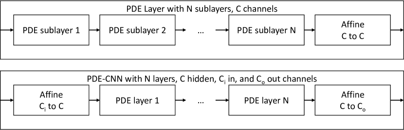
By concatenating various PDE sublayers, that being either a sublayer that correspond to a scale-space or a convection sublayer, with an affine combination layer at the end we form a PDE layer. Multiple PDE layers after each other with an affine layer in the start and end creates a PDE-CNN. The architecture is illustrated in Figure 8

Figure 8: The architecture of a $N$-layer PDE-CNN with $C$ channels. A PDE sublayer is either of the form (25) or (26).

6.2 Data Efficiency of PDE-CNNs on DRIVE dataset

The data efficiency of PDE-G-CNNs is already verified in [3], but if this desirable property this holds in the PDE-CNN case is still left untested. Our first experiment is therefor testing the data efficiency of a PDE-CNN. The PDE-CNN we consider here employs three PDEs within its PDE layers: convection, $\alpha$-dilation, and $\alpha$-erosion, just as in the papers [1, 4, 5, 3].

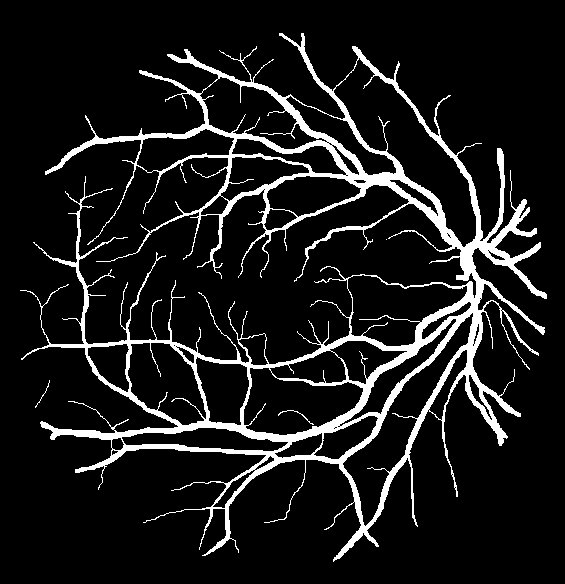
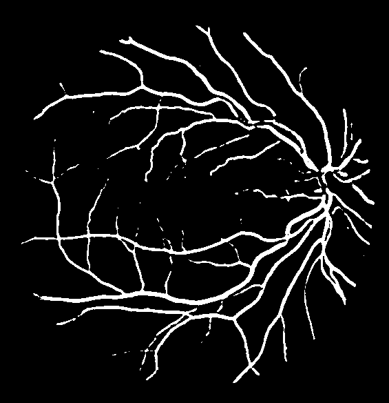
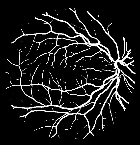
We will be testing on the DRIVE dataset [14], which consists of $584\times 565$ 8bit RGB color fundus images, with the goal being vessel segmentation. In Figure 9 one can see an example of such an image and its segmentation. The dataset consist of a training set of $20$ images, and a test set of $20$ images. All images are rescaled within the $[0,1]$ range by dividing by $255$. We divided the training set into $2\,880$ overlapping patches of $64\times 64$. Patches that contain no annotation, i.e. patches that are essentially completely within the black mask, are removed, leaving us with $2\,409$ patches.

(a) Input image of the fundus of the eye.

(b) Target vessel segmentation.

(c) Example output of a network with a dice coefficient of $\approx 0.78$. Notice how small vessels are missed.

(d) Example output of a network with a dice coefficient of $\approx 0.81$. Notice how more small vessels are captured.

Figure 9: One instance of an input and its corresponding target segmentation from the DRIVE dataset, together with two example outputs of networks with different dice coefficients.

As a baseline we consider a $6$-layer CNN with $25\,662$ parameters from [3], and compare this against a $6$-layer $24$-channel PDE-CNN with $5\,280$ parameters. These networks have been designed to give a satisfactory Dice coefficient of $\gtrapprox 0.80$ on the test set when trained on the complete training set.

Following the method in [3], we randomly take $1\%$ to $100\%$ of the training data. We train on batches consisting of $8$ patches. We empirically found that a higher batch size results in a worse test set accuracy. We use the AdamW optimizer with an initial learning rate of $0.01$ that decays linearly to $0.001$ over the first $1\,000$ batches. The beta, epsilon and weight decay parameters of AdamW are kept at their default values of $(0.9,0.999)$, $10^{-8}$, and $0.01$. During training we keep track of the Dice coefficient on the test set and the best one is stored. We train until this performance on the test test no longer increases, which happens within $15\,000$ batches. We repeat this 5 times for every possible situation to obtain an average performance.

The result can be found in Figure 10. We see that on the DRIVE dataset, in comparison with a standard CNN, the PDE-CNN not only features fewer parameters but also showcases competitive performance and increased data efficiency. This mirrors the results found in [3], but this time for a PDE-CNN instead of the $G=\text{SE}(2)$ PDE-G-CNN considered there.

Figure 10: A scatterplot of the performance of a 6-layer CNN ($25\,662$ parameters) and PDE-CNN ($5\,280$ parameters) on the DRIVE dataset, when trained multiple times on varying amounts of training data. The crosses indicate the mean.

6.3 Other Semifields within PDE-CNNs

The second experiment examines how including the discussed semifields affects performance. This means we add PDE sublayers corresponding to the scale-spaces (Definition 28) that arise naturally from the semifields, as shown in Theorem 1. To keep focus we only consider semifields we have already discussed, that being the linear $L$, tropical min ${T_{\scalebox{0.6}{$-$}}}$, tropical max ${T_{\scalebox{0.6}{$+$}}}$, root $R_{p}$, and logarithmic $L_{\mu}$ semifields. In concrete terms, this means we implement the scale-spaces listed in Definition 29.

The networks that we consider always include the convection PDE sublayer at the start of the PDE layer. The PDE-CNNs will always consist of 6 PDE layers, 32 channels, and have parameter count of approximately $9\,500$ on average, which changes with the amount of semifields we add.

Our methodology is identical to Section 6.2, however this time we always train on the complete DRIVE dataset. This allows us to compare the results found in this section with the ones in Figure 10. We found that training is a bit slower with the logarithmic and root semifields, so we increased the training to $20\,000$ batches.

We empirically found that adding the linear semifield, that is we add a PDE sublayer corresponding to the Gaussian scale-space, does not affect the performance of any the networks. This can be explained by noticing that such a PDE sublayer can be emulated completely and effectively by the convection sublayer together with the affine combination sublayer, which are always components of the PDE-CNNs we consider here. For this reason we have omitted the linear semifield PDE sublayers altogether. This is in agreement with the results found in [47, p.28].

The result can be found in Figure 11. We observe multiple things:

• Adding semifields to the existing PDE-CNN architecture, which only employ the tropical semifields and convection, may enhance performance, albeit not significantly, as observed in the case of $\{{T_{\scalebox{0.6}{$+$}}},{T_{\scalebox{0.6}{$-$}}},L_{\mu}\}$.

• The inclusion of the tropical min semifield ${T_{\scalebox{0.6}{$-$}}}$ always increases performance, most starkly seen when going from $\{L_{\mu}\}$ to $\{{T_{\scalebox{0.6}{$-$}}},L_{\mu}\}$.

• Adding semifields does not necessarily improve performance, as is evident from the last row when compared to the two-semifield models in the middle rows.

• The inclusion of the root semifield $R_{p}$ seems to make the training less stable, as indicated by the increase in spread within the scatter plot at the respective rows.

It is worth mentioning however that these results might be specific to the DRIVE dataset.

Semifield
${T_{\scalebox{0.6}{$+$}}}$	${T_{\scalebox{0.6}{$-$}}}$	$L_{\mu}$	$R_{p}$
✓	✗	✗	✗
✗	✓	✗	✗
✗	✗	✓	✗
✗	✗	✗	✓
✓	✓	✗	✗
✓	✗	✓	✗
✓	✗	✗	✓
✗	✓	✓	✗
✗	✓	✗	✓
✗	✗	✓	✓
✓	✓	✓	✗
✓	✓	✗	✓
✓	✗	✓	✓
✗	✓	✓	✓
✓	✓	✓	✓

Figure 11: A scatterplot of the performance of a 6-layer PDE-CNN on the DRIVE dataset, with various designs of the PDE layer as indicated in the table on the left. The crosses indicate the mean. The rows are organized according to the amount of semifields included in the model.

7 Conclusion

PDE-CNNs are an interesting alternative to CNNs in the sense that their constituents, this being solvers of PDEs that generate scale-spaces, are geometrically meaningful and interpretable.

The existing PDE-CNN framework utilizes four PDEs: convection, diffusion, dilation, and erosion. Through the introduction of semifield scale-spaces, we demonstrate the presence of a broad class of PDEs that remain unutilized within the PDE-CNN paradigm.

The theory of semifields scale-spaces is expressive and encapsulates a large class of known scale-spaces. Theorem 1 shows that every semifield gives rise to a one-parameter family of semifield scale-spaces. This indicates that the generalization to semifields is one that is not too general and definitely fruitful.

In Section 6.2 we empirically verified that on the DRIVE dataset that PDE-CNNs, just like PDE-G-CNNs, when compared to traditional CNNs, require less training data, have fewer parameters, and increased performance.

We experimented on the inclusion of various semifields and their corresponding scale-spaces within PDE layers of a PDE-CNN. We see that the thought “more semifields means better performance” is incorrect, and that it is not clear if the addition of more semifields into the already existing PDE-CNN framework is worth the effort. However, in all cases inclusion of the tropical semifield improved the result, advocating for tropical algebras in PDE-based neural networks.

Further Research

When comparing the results of PDE-CNNs on the DRIVE dataset here to the $G=\text{SE}(2)$ PDE-G-CNNs results in [3], the accuracy is essentially the same (Dice $\approx 0.81$), but there is a trade-off between memory usage and parameter reduction. The $\text{SE}(2)$ variant has less parameters ($2\,560$) but, due to the feature maps being scalar fields on $\text{SE}(2)$, uses more memory. Conversely, the $\mathbb{R}^{2}$ variant has more parameters ($5\,280$) but uses much less memory. This means that in some applications the PDE-CNN might be preferable. However, the goal of the work here was not to compare PDE-CNNs to PDE-G-CNNs and the observations here only apply to the DRIVE dataset. Further research is needed to properly compare both architectures.

Acknowledgements

We thank Adrien Castella [47] for the initial Python implementation of the $\mathbb{R}^{2}$ convection, diffusion, dilation and erosion PDE sublayers https://github.com/adrien-castella/PDE-based-CNNs.

Declarations

Funding

We gratefully acknowledge the Dutch Foundation of Science NWO for funding of VICI 2020 Exact Sciences (Duits, Geometric learning for Image Analysis, VI.C. 202-031).

Availability of Data and Code

The DRIVE dataset [14] can (currently) be found at https://drive.grand-challenge.org/. The LieTorch package is public and can be found at https://gitlab.com/bsmetsjr/lietorch. The original PDE-CNN implementation can be found at https://github.com/adrien-castella/PDE-based-CNNs.

Appendix A Semifield Fourier Transforms

Lemma 11.

The employed semifield Fourier transforms indeed satisfy Definition 26.

Proof.

In the linear semifield $L$ case we know that the familiar Fourier transform satisfies the definition.

As for the root and logarithmic semifields, being isomorphic to the linear semifield, we can quickly deduce that they also satisfy the definitions through the equalities

$$\begin{split}\mathcal{F}_{L_{\mu}}&=\mathcal{P}_{\varphi_{\mu}^{-1}}\circ\mathcal{F}_{L}\circ\mathcal{P}_{\varphi_{\mu}},\\ \mathcal{F}_{R_{p}}&=\mathcal{P}_{\varphi_{p}^{-1}}\circ\mathcal{F}_{L}\circ\mathcal{P}_{\varphi_{p}},\end{split}$$

where $\mathcal{P}$ is the pointwise operator (9), $\varphi_{\mu}(x)=e^{\mu x}$ the semifield isomorphism $\varphi_{\mu}:L_{\mu}\to L_{\geq 0}$, and $\varphi_{p}(x)=x^{p}$ the semifield isomorphism $\varphi_{p}:R_{p}\to L_{\geq 0}$. For example, to show that $\mathcal{F}_{L_{\mu}}$ satisfies the convolution property:

$$\begin{split}&\mathcal{F}_{L_{\mu}}(f\circledast g)\\ &=\mathcal{P}_{\varphi_{\mu}^{-1}}\mathcal{F}_{L}\mathcal{P}_{\varphi_{\mu}}(f\circledast g)\\ &=\mathcal{P}_{\varphi_{\mu}^{-1}}\mathcal{F}_{L}((\mathcal{P}_{\varphi_{\mu}}f)*(\mathcal{P}_{\varphi_{\mu}}g))\\ &=\mathcal{P}_{\varphi_{\mu}^{-1}}((\mathcal{F}_{L}\mathcal{P}_{\varphi_{\mu}}f)\times(\mathcal{F}_{L}\mathcal{P}_{\varphi_{\mu}}g))\\ &=(\mathcal{P}_{\varphi_{\mu}^{-1}}\mathcal{F}_{L}\mathcal{P}_{\varphi_{\mu}}f)\otimes(\mathcal{P}_{\varphi_{\mu}^{-1}}\mathcal{F}_{L}\mathcal{P}_{\varphi_{\mu}}g)\\ &=(\mathcal{F}_{L_{\mu}}f)\otimes(\mathcal{F}_{L_{\mu}}g),\end{split}$$

where $\circledast$ and $\otimes$ are the semifield convolution and multiplication of $L_{\mu}$ and where $\times$ denotes the standard pointwise product of functions. In the above derivation we have used that

$$\begin{split}\mathcal{P}_{\varphi_{\mu}}(f\circledast g)&=(\mathcal{P}_{\varphi_{\mu}}f)*(\mathcal{P}_{\varphi_{\mu}}g),\\ \mathcal{P}_{\varphi_{\mu}^{-1}}(f\times g)&=(\mathcal{P}_{\varphi_{\mu}^{-1}}f)\otimes(\mathcal{P}_{\varphi_{\mu}^{-1}}g),\end{split}$$

and that $\mathcal{F}_{L}$ has the convolution property.

Consider now the tropical max semifield ${T_{\scalebox{0.6}{$+$}}}$. That $\mathcal{F}_{T_{\scalebox{0.6}{$+$}}}$ satisfies the linearity, equivariances, and the zero-frequency properties is immediate. As for the convolution property we have

$$\begin{split}&(\mathcal{F}_{{T_{\scalebox{0.6}{$+$}}}}(f\circledast g))(\omega)\\ &=\sup_{x}\ (f\circledast g)(x)-\omega\cdot x\\ &=\sup_{x}\ (\sup_{y}f(x-y)+g(y))-\omega\cdot x\\ &=\sup_{x}\ (\sup_{x_{1}+x_{2}=x}f(x_{1})+g(x_{2}))-\omega\cdot x\\ &=\sup_{x_{1},x_{2}}\ f(x_{1})+g(x_{2})-\omega\cdot(x_{1}+x_{2})\\ &=(\sup_{x_{1}}f(x_{1})-\omega\cdot x_{1})+(\sup_{x_{2}}g(x_{2})-\omega\cdot x_{2})\\ &=(\mathcal{F}_{{T_{\scalebox{0.6}{$+$}}}}f)(\omega)\otimes(\mathcal{F}_{{T_{\scalebox{0.6}{$+$}}}}g)(\omega),\end{split}$$

where $\otimes$ and $\circledast$ are the tropical max ${T_{\scalebox{0.6}{$+$}}}$ multiplication and convolution. For the invertibility we refer to the Fenchel biconjugation theorem [48, Thm.4.2.1]. That the tropical min semifield Fourier transform $\mathcal{F}_{T_{\scalebox{0.6}{$-$}}}$ satisfies all properties follows from the fact that ${T_{\scalebox{0.6}{$-$}}}$ is semifield isomorphic to ${T_{\scalebox{0.6}{$+$}}}$ with the isomorphism being $\phi(x)=-x$. ∎

Appendix B Tropical Integration

Proposition 4.

The natural integration of sum-approachable and bounded from above functions $f:\mathbb{R}^{2}\to{T_{\scalebox{0.6}{$+$}}}$ is

$$\oint^{{T_{\scalebox{0.6}{$+$}}}}f=\sup_{x\in\mathbb{R}^{2}}f(x).$$

The natural integration of sum-approachable and bounded from below functions $f:\mathbb{R}^{2}\to{T_{\scalebox{0.6}{$-$}}}$ is

$$\oint^{{T_{\scalebox{0.6}{$-$}}}}f=\inf_{x\in\mathbb{R}^{2}}f(x).\\$$

Proof.

We will only prove this for the tropical max semifield ${T_{\scalebox{0.6}{$+$}}}$, the tropical min semifield case goes completely analogously. As we are working with ${T_{\scalebox{0.6}{$+$}}}$ we remind ourselves that we have $\oplus=\max$, $\otimes=+$, $\mu_{{T_{\scalebox{0.6}{$+$}}}}(A)=0$, and

$$\mathbb{1}_{A}(x)=\begin{cases}0&\text{ if }x\in A\\ -\infty&\text{ otherwise }\end{cases}.$$

The function $f$, being sum-approachable and bounded from above, is pointwise defined by the limit

$$f(x)=\lim_{n\to\infty}\bigoplus_{i=1}^{n}a_{i}\otimes\mathbb{1}_{A_{i}}(x),$$

with $A_{i}$ non-empty and $a_{i}$ bounded from above. We define its natural integral by

$$\begin{split}\oint f&:=\lim_{n\to\infty}\oint\left(\bigoplus_{i=1}^{n}a_{i}\otimes\mathbb{1}_{A_{i}}\right)\\ &=\lim_{n\to\infty}\bigoplus_{i=1}^{n}a_{i}\otimes\mu(A)\\ &=\lim_{n\to\infty}\max_{i=1,\dots,n}a_{i}+0\\ &=\sup_{i\in\mathbb{N}}a_{i},\\ \end{split}$$

where the second equality is by the linearity of the integration (10) and the indicator function property (11).

Similarly, we have

$$\begin{split}\sup_{x\in\mathbb{R}^{2}}f(x)&=\sup_{x\in\mathbb{R}^{2}}\lim_{n\to\infty}\bigoplus_{i=1}^{n}a_{i}\otimes\mathbb{1}_{A_{i}}(x)\\ &=\sup_{x\in\mathbb{R}^{2}}\lim_{n\to\infty}\max_{i=1,\dots,n}a_{i}+\mathbb{1}_{A_{i}}(x)\\ &=\sup_{x\in\mathbb{R}^{2}}\sup_{i\in\mathbb{N}}a_{i}+\mathbb{1}_{A_{i}}(x)\\ &=\sup_{i\in\mathbb{N}}\sup_{x\in\mathbb{R}^{2}}a_{i}+\mathbb{1}_{A_{i}}(x)\\ &=\sup_{i\in\mathbb{N}}a_{i},\end{split}$$

where in the fourth equality we interchanged the order of suprema, and in the fifth equality we used the definition of $\mathbb{1}_{A_{i}}$.

Combining these two results, it follows that

$$\oint f=\sup_{x\in\mathbb{R}^{2}}f(x)$$

is the natural tropical max semifield integration. ∎

References

- \bibcommenthead
- [1] Smets, B., Portegies, J., Bekkers, E. & Duits, R. PDE-based group equivariant convolutional neural networks. Journal of Mathematical Imaging and Vision 65, 209–239 (2023). 10.1007/s10851-022-01114-x.
- [2] Cohen, T. & Welling, M. Balcan, M. F. & Weinberger, K. Q. (eds) Group equivariant convolutional networks. (eds Balcan, M. F. & Weinberger, K. Q.) Proceedings of The 33rd International Conference on Machine Learning, Vol. 48 of Proceedings of Machine Learning Research, 2990–2999 (PMLR, New York, New York, USA, 2016). URL https://proceedings.mlr.press/v48/cohenc16.html.
- [3] Pai, G., Bellaard, G., Smets, B. & Duits, R. Nielsen, F. & Barbaresco, F. (eds) Functional properties of PDE-based group equivariant convolutional neural networks. (eds Nielsen, F. & Barbaresco, F.) Geometric Science of Information, 63–72 (Springer Nature Switzerland, Cham, 2023). 10.1007/978-3-031-38271-0_7.
- [4] Bellaard, G., Bon, D., Pai, G., Smets, B. & Duits, R. Analysis of (sub-)Riemannian PDE-G-CNNs. Journal of Mathematical Imaging and Vision 65, 819–843 (2023). 10.1007/s10851-023-01147-w.
- [5] Bellaard, G., Pai, G., Bescos, J. & Duits, R. Calatroni, L., Donatelli, M., Morigi, S., Prato, M. & Santacesaria, M. (eds) Geometric adaptations of PDE-G-CNNs. (eds Calatroni, L., Donatelli, M., Morigi, S., Prato, M. & Santacesaria, M.) Scale Space and Variational Methods in Computer Vision, 538–550 (Springer International Publishing, Cham, 2023). 10.1007/978-3-031-31975-4_41.
- [6] Field, D., Hayes, A. & Hess, R. Contour integration by the human visual system: Evidence for a local “association field”. Vision Research 33, 173–193 (1993). 10.1016/0042-6989(93)90156-Q.
- [7] Petitot, J. The neurogeometry of pinwheels as a sub-Riemannian contact structure. Journal of Physiology - Paris 97, 265–309 (2003). 10.1016/j.jphysparis.2003.10.010.
- [8] Citti, G. & Sarti, A. A cortical based model of perceptional completion in the roto-translation space. Journal of Mathematical Imaging and Vision 24, 307–326 (2006). 10.1007/s10851-005-3630-2.
- [9] Haar Romeny, B. Front-End Vision and Multi-Scale Image Analysis (Springer Dordrecht, 2003). 10.1007/978-1-4020-8840-7.
- [10] Iijima, T. Basic theory of pattern observation. Papers of Technical Group on Automata and Automatic Control (1959).
- [11] Weickert, J., Ishikawa, S. & Imiya, A. Linear scale-space has first been proposed in japan. Journal of Mathematical Imaging and Vision 10, 237–252 (1999). 10.1023/A:1008344623873.
- [12] Koenderink, J. The structure of images. Biological Cybernetics 50, 363–370 (1984). 10.1007/BF00336961.
- [13] Brockett, R. & Maragos, P. IEEE (ed.) Evolution equations for continuous-scale morphology. (ed.IEEE) 1992 IEEE International Conference on Acoustics, Speech, and Signal Processing, Vol. 3, 125–128 vol.3 (IEEE, 1992). 10.1109/ICASSP.1992.226260.
- [14] Staal, J., Abramoff, M., Niemeijer, M., Viergever, M. & van Ginneken, B. Ridge-based vessel segmentation in color images of the retina. IEEE Transactions on Medical Imaging 23, 501–509 (2004). 10.1109/TMI.2004.825627.
- [15] Evans, L. Partial Differential Equations Graduate studies in mathematics (American Mathematical Society, 2010). 10.1090/gsm/019.
- [16] Mohamed, M., Cesa, G., Cohen, T. & Welling, M. A data and compute efficient design for limited-resources deep learning (2020). 10.48550/arXiv.2004.09691.
- [17] Cohen, T., Weiler, M., Kicanaoglu, B. & Welling, M. Chaudhuri, K. & Salakhutdinov, R. (eds) Gauge equivariant convolutional networks and the icosahedral CNN. (eds Chaudhuri, K. & Salakhutdinov, R.) Proceedings of the 36th International Conference on Machine Learning, Vol. 97, 1321–1330 (PMLR, 2019). URL https://proceedings.mlr.press/v97/cohen19d.html.
- [18] Sosnovik, I., Szmaja, M. & Smeulders, A. ICLR (ed.) Scale-equivariant steerable networks. (ed.ICLR) International Conference on Learning Representations (ICLR, 2020). URL https://openreview.net/forum?id=HJgpugrKPS.
- [19] Lindeberg, T. Scale-covariant and scale-invariant gaussian derivative networks. Journal of Mathematical Imaging and Vision 64, 223–242 (2022). 10.1007/s10851-021-01057-9.
- [20] Worrall, D. & Welling, M. Wallach, H. et al. (eds) Deep scale-spaces: Equivariance over scale. (eds Wallach, H. et al.) Advances in Neural Information Processing Systems, Vol. 32 (Curran Associates, Inc., 2019). URL https://proceedings.neurips.cc/paper_files/paper/2019/file/f04cd7399b2b0128970efb6d20b5c551-Paper.pdf.
- [21] Sangalli, M., Blusseau, S., Velasco-Forero, S. & Angulo, J. Lindblad, J., Malmberg, F. & Sladoje, N. (eds) Scale equivariant neural networks with morphological scale-spaces. (eds Lindblad, J., Malmberg, F. & Sladoje, N.) Discrete Geometry and Mathematical Morphology, 483–495 (Springer International Publishing, Cham, 2021). 10.1007/978-3-030-76657-3_35.
- [22] Pauwels, E., van Gool, L., Fiddelaers, P. & Moons, T. An extended class of scale-invariant and recursive scale space filters. IEEE Transactions on Pattern Analysis and Machine Intelligence 17, 691–701 (1995). 10.1109/34.391411.
- [23] Duits, R., Florack, L., Haar Romenij, B. & Graaf, H. Younan, N. (ed.) Scale-space axioms critically revisited. (ed.Younan, N.) Proceedings of the Fourth IASTED International Conference on Signal and Image Processing (SIP’2002, Kauai HI, USA, August 2002), 304–309 (ACTA Press, Canada, 2002).
- [24] Welk, M. Griffin, L. & Lillholm, M. (eds) Families of generalised morphological scale spaces. (eds Griffin, L. & Lillholm, M.) Scale Space Methods in Computer Vision, 770–784 (Springer Berlin Heidelberg, Berlin, Heidelberg, 2003). 10.1007/3-540-44935-3_54.
- [25] Schmidt, M. & Weickert, J. Morphological counterparts of linear shift-invariant scale-spaces. Journal of Mathematical Imaging and Vision 56, 352–366 (2016). 10.1007/s10851-016-0646-8.
- [26] Heijmans, H. & Boomgaard, R. Algebraic framework for linear and morphological scale-spaces. Journal of Visual Communication and Image Representation 13, 269–301 (2002). 10.1006/jvci.2001.0480.
- [27] Fathi, A. & Maderna, E. Weak KAM theorem on non compact manifolds. Nonlinear Differential Equations and Applications NoDEA 14, 1–27 (2007). 10.1007/s00030-007-2047-6.
- [28] Azagra, D., Ferrera, J. & López-Mesas, F. Nonsmooth analysis and Hamilton–Jacobi equations on Riemannian manifolds. Journal of Functional Analysis 220, 304–361 (2005). 10.1016/j.jfa.2004.10.008.
- [29] Alvarez, L., Guichard, F., Lions, P. & Morel, J. Axioms and fundamental equations of image processing. Archive for Rational Mechanics and Analysis 123, 199–257 (1993). 10.1007/BF00375127.
- [30] Sapiro, G. Geometric Partial Differential Equations and Image Analysis (Cambridge University Press, 2001). 10.1017/CBO9780511626319.
- [31] Citti, G., Franceschiello, B., Sanguinetti, G. & Sarti, A. Sub-riemannian mean curvature flow for image processing. SIAM Journal on Imaging Sciences 9, 212–237 (2016). 10.1137/15M1013572.
- [32] Guichard, F. & Morel, J. Duff, I. & Watson, G. (eds) Partial differential equations and image iterative filtering. (eds Duff, I. & Watson, G.) The State of the Art in Numerical Analysis., Vol. 63, 252–562 (Clarendon Press, 1997). 10.1093/oso/9780198500148.003.0020.
- [33] Feller, W. An Introduction to Probability Theory and its Applications Vol. II (Wiley, New York, 1971).
- [34] Dorst, L. & Boomgaard, R. Morphological signal processing and the slope transform. Signal Processing 38, 79–98 (1994). 10.1016/0165-1684(94)90058-2.
- [35] Florack, L. Non-linear scale-spaces isomorphic to the linear case with applications to scalar, vector and multispectral images. International Journal of Computer Vision 42, 39–53 (2001). 10.1023/A:1011185417206.
- [36] Felsberg, M. & Sommer, G. The monogenic scale-space: A unifying approach to phase-based image processing in scale-space. Journal of Mathematical Imaging and Vision 21, 5–26 (2004). 10.1023/B:JMIV.0000026554.79537.35.
- [37] Duits, R., Florack, L., de Graaf, J. & Haar Romenij, B. On the axioms of scale space theory. Journal of Mathematical Imaging and Vision 20, 267–298 (2004). 10.1023/B:JMIV.0000024043.96722.aa.
- [38] Yosida, K. Functional Analysis (Springer Berlin, Heidelberg, 1965). 10.1007/978-3-662-25762-3.
- [39] Burgeth, B. & Weickert, J. An explanation for the logarithmic connection between linear and morphological system theory. International Journal of Computer Vision 64, 157–169 (2005). 10.1007/s11263-005-1841-z.
- [40] Akian, M., Quadrat, J. & Viot, M. Cohen, G. & Quadrat, J. (eds) Bellman processes. (eds Cohen, G. & Quadrat, J.) 11th International Conference on Analysis and Optimization of Systems Discrete Event Systems, 302–311 (Springer Berlin Heidelberg, Berlin, Heidelberg, 1994). 10.1007/BFb0033561.
- [41] Pin, J.-E. in Tropical Semirings (ed.Gunawardena, J.) Idempotency (Bristol, 1994) Publ. Newton Inst. 11, 50–69 (Cambridge Univ. Press, Cambridge, 1998). URL https://hal.science/hal-00113779.
- [42] Kolokoltsov, V. & Maslov, V. Idempotent Analysis and Its Applications (Springer Dordrecht, 1997). 10.1007/978-94-015-8901-7.
- [43] saz. Measurability of a pointwise limit of measurable functions. Mathematics Stack Exchange. URL https://math.stackexchange.com/q/921576.
- [44] Matematleta. a proof that the pointswise limits of lower semicontinuous (lsc) functions is lsc. Mathematics Stack Exchange. URL https://math.stackexchange.com/q/2968282.
- [45] Rudin, W. Functional Analysis (McGraw-Hill, 1973, 1991).
- [46] Kraakman, T. B. On the Construction of Classical and Quantum PDE-Based Neural Networks. Master’s thesis, Eindhoven University of Technology (2023).
- [47] Castella, A. Introduction to Shift-Invariant PDE-based Convolutional Neural Networks and experimentation with Vessel Segmentation. Bachelor’s thesis, Eindhoven University of Technology (2021).
- [48] Borwein, J. & Lewis, A. Convex Analysis and Nonlinear Optimization (Springer New York, NY, 2016). 10.1007/978-0-387-31256-9.