Self-Improvement for Neural Combinatorial Optimization:
Sample without Replacement, but Improvement

Abstract

Current methods for end-to-end constructive neural combinatorial optimization usually train a policy using behavior cloning from expert solutions or policy gradient methods from reinforcement learning. While behavior cloning is straightforward, it requires expensive expert solutions, and policy gradient methods are often computationally demanding and complex to fine-tune. In this work, we bridge the two and simplify the training process by sampling multiple solutions for random instances using the current model in each epoch and then selecting the best solution as an expert trajectory for supervised imitation learning. To achieve progressively improving solutions with minimal sampling, we introduce a method that combines round-wise Stochastic Beam Search with an update strategy derived from a provable policy improvement. This strategy refines the policy between rounds by utilizing the advantage of the sampled sequences with almost no computational overhead. We evaluate our approach on the Traveling Salesman Problem and the Capacitated Vehicle Routing Problem. The models trained with our method achieve comparable performance and generalization to those trained with expert data. Additionally, we apply our method to the Job Shop Scheduling Problem using a transformer-based architecture and outperform existing state-of-the-art methods by a wide margin.

1 Introduction

Several learning-based methods have been proposed for solving combinatorial optimization (CO) problems in recent years. These neural approaches aim to enable a deep neural network to learn how to generate heuristics without manual crafting. A prominent paradigm in this direction is the constructive approach, where a solution to a problem instance is built step by step as a sequential decision problem. A neural network models the policy that guides these incremental decisions. It is trained by supervised learning (SL) using expert solutions as labeled data (Vinyals et al., 2015; Joshi et al., 2019; Fu et al., 2021; Kool et al., 2022; Hottung et al., 2020; Drakulic et al., 2023; Luo et al., 2023) or by reinforcement learning (RL) (Bello et al., 2016; Kool et al., 2019b; Nazari et al., 2018; Chen & Tian, 2019; Ahn et al., 2020; d O Costa et al., 2020; Hottung & Tierney, 2020; Kwon et al., 2020; Ma et al., 2021; Kim et al., 2021; Park et al., 2021; Wu et al., 2021; Park et al., 2022; Zhang et al., 2020; Hottung et al., 2022; Zhang et al., 2024), which exploits the natural modeling of the sequential problem as a finite Markov decision process. While obtaining expert solutions from (exact) solvers can be expensive for SL-based methods, RL-based methods, especially policy gradient methods, can be challenging to train due to high memory requirements and strong hyperparameter sensitivity (Schulman et al., 2017; Henderson et al., 2018). Recent work attributes the poor ability of current methods to generalize to larger instances than those seen during training to the typically lightweight decoder of the used architectures (Drakulic et al., 2023; Luo et al., 2023). Increasing the size of the decoder structure can address this issue, but makes it impractical to train the model with policy gradient methods due to the increased computational cost.

In this paper, we move away from RL for neural CO towards a simple, problem-independent training scheme derived from the Cross-Entropy Method (CEM) (De Boer et al., 2005): We sample a set of solutions for randomly generated problem instances in each epoch using the current model. The sampled solution with the best objective function evaluation for each instance is treated as a pseudo-expert trajectory on which we can train the model in a supervised manner. By repeatedly ’self-imitating’ the best solutions found, we create an improving loop.

The effectiveness of this strategy relies on the quality of the sampled solutions and the efficiency of the sampling process. In particular, we want to sample as few sequences as possible to get better and better solutions in each epoch. Simple repeated sampling from the conditional distribution given by the model at each sequential step can result in a set of sequences that lacks diversity, contains numerous duplicates, and requires a large number of samples to find a solution that enables the network to improve. This paper utilizes a sampling mechanism based on batch-wise Stochastic Beam Search (SBS) (Kool et al., 2019c) as introduced by (Shi et al., 2020). The mechanism draws samples without replacement in multiple rounds while maintaining a search tree. We suggest taking advantage of the batch- and round-wise mechanism to enhance its effectiveness. Given the sequences sampled in a single round, we estimate the expected value of the objective function and update the trie with the advantage of the sampled sequences, a strategy derived from a provable policy improvement operation. Furthermore, to balance the explore-exploit tradeoff, we couple this update strategy with Top-$p$ (nucleus) sampling (Holtzman et al., 2020). We gradually increase $p\leq 1$ after each round to allow more unreliable sequences. Our method applies to any constructive neural CO problem, unlike sampling strategies that leverage problem specifics to diversify and improve the sampled solutions (Kwon et al., 2020).

On the Traveling Salesman Problem (TSP) and the Capacitated Vehicle Routing Problem (CVRP), we demonstrate that training state-of-the-art architectures with our introduced method Gumbeldore (GD) can produce policies of comparable strength to those trained with expert trajectories from solvers. In addition, we train a transformer-based architecture for the classical Job Shop Scheduling Problem (JSSP) using our method. Our results outperform the current state of the art by a wide margin.

Our contributions are summarized as follows:

(i) For constructive neural combinatorial optimization, we propose to sample diverse sequences without replacement from the current model and use the best sequences as pseudo-expert trajectories to imitate.

(ii) We draw the sequences in multiple rounds using batch-wise SBS. We develop a technique to make the underlying search tree more informed in each round by updating the sequence probabilities according to their advantage. Informally, we increase (decrease) the probability of better (worse) trajectories than expected. This update adds next to no computational overhead to the sampling method, and we derive this technique from a provable policy improvement.

(iii) We couple SBS with Top-$p$ sampling, where we start with $p<1$ and increase to $p=1$ over the rounds of sampling. While putting pressure on the model to disregard unreliable choices with a low $p$ works well in confident models, exploiting the model in such a way can hurt the performance in the early stages of training when the model itself is unreliable. By covering a range of $p$, we compromise between both cases.

(iv) We show on the TSP and CVRP that we can achieve comparable results to direct training on (near) optimal expert trajectories. We further present a pure self-attention architecture for JSSP that outperforms the current state of the art when trained with our method.

Our code for the experiments, data, and trained network weights are available at https://github.com/grimmlab/gumbeldore.

2 Related Work

Learning constructive heuristics

Initiated by Vinyals et al. (2015) and Bello et al. (2016), the constructive approach in neural CO uses a neural network (policy) to incrementally build solutions by selecting one element at a time. The most prominent way to train the policy network without relying on labeled data has become policy gradient methods in RL, notably using REINFORCE (Williams, 1992) with self-critical training (Rennie et al., 2017), where the result of a greedy rollout is used as a baseline for the gradient (Kool et al., 2019b). A large body of research focuses on keeping the network architecture fixed and instead improving the self-critical baseline and gradient estimation by diversifying the sampled solutions (Kool et al., 2019a; Kwon et al., 2020; Kool et al., 2020; Kim et al., 2021; 2022), often by exploiting problem-specific symmetries. For example, POMO (Kwon et al., 2020), one of the strongest constructive approaches, achieves diversity in routing problems by rolling out the model from all possible starting nodes of an instance. For the policy network, the Transformer (Vaswani et al., 2017) has become the standard choice for many CO problems (Deudon et al., 2018; Kool et al., 2019b; Kwon et al., 2020; Zhao et al., 2022) and is also used extensively in this work. However, current RL-based methods struggle to generalize to larger instances (Joshi et al., 2020), possibly due to their prevalent encoder-decoder structure, where a heavy encoder and light decoder facilitate training with policy gradient methods but limit scalability. On the other hand, recent work suggests that a lighter encoder with a heavier decoder can significantly improve generalization results (even with greedy inference only) (Drakulic et al., 2023; Luo et al., 2023), albeit at the cost of increased (if not prohibitive) computational complexity for training with RL.

Self-imitation in neural CO

The CEM (De Boer et al., 2005; Rubinstein, 1999) is a derivative-free optimization technique that can be summarized as generating a set of solution candidates, evaluating them according to some objective function, and selecting the best-performing candidates to guide the generation of new solutions. While this principle of pushing the policy toward better performing sampled solutions lies at the heart of the self-critical policy gradient methods, there is little work on directly cloning the behavior of trajectories sampled from the current model in neural CO (Bogyrbayeva et al., 2022; Bengio et al., 2021). In fact, independent of our work, Corsini et al. (2024) make the same observation. They present a ’self-labeling’ strategy that samples multiple solutions from the current policy and uses the best one as a pseudo-label for supervised training. However, they focus only on the JSSP and use vanilla sampling with replacement, in contrast to our main contribution, which updates the policy during the sampling without replacement process. We refer to Appendix E for a deeper comparison. Furthermore, Luo et al. (2023) show a hybrid problem-specific way to learn without any labeled data by pre-training a randomly initialized model with RL on small instances, followed by reconstructing partial solutions to refine an unlabeled training dataset. We show that we can outperform this strategy without relying on RL.

Improving at inference time

Closely related to our proposed sampling methods are approaches that use inference-time search methods (other than greedy and pure beam search) to improve the generated solutions. While the aforementioned problem-specific diversification of POMO falls into this category, Choo et al. (2022) propose a beam search guided by greedy rollouts. Active Search (Bello et al., 2016) and EAS (Hottung et al., 2022) update (a subset of) the policy network parameters for individual instances using gradient descent. The tabular version of EAS is reminiscent of our approach by forcing sampled solutions to be close to the best solution found so far. MDAM (Xin et al., 2021) and Poppy (Grinsztajn et al., 2024) maintain a population of policies, while COMPASS (Chalumeau et al., 2024) learns a distribution of policies that is searched at test time. However, these search methods are designed only for test time to exploit a pre-trained model or require a significant computational budget on the order of minutes per instance. This makes them impractical in our self-improving setting, where we require trajectories that may live for only one epoch.

3 Learning Algorithm

In the following section, we formally set up the problem and present our method’s overarching simple learning algorithm.

3.1 Problem Setup

This paper considers a CO problem with $T\in\mathbb{N}$ decision variables of finite domain. Let $\mathcal{X}$ be some distribution over the problem instances. For each instance $x\sim\mathcal{X}$, we assume that we can construct a feasible solution sequentially by assigning a value $a_{1}$ to the first variable, then $a_{2}$ to the second, and so on, until we arrive at a complete trajectory $\bm{a}_{1:T}:=(a_{1},\dots,a_{T})\in\mathcal{S}_{x}$, where $\mathcal{S}_{x}$ is the set of all feasible solutions. Given an objective function $f_{x}\colon\mathcal{S}_{x}\to\mathbb{R}$ that maps a feasible solution to a real scalar, the goal is to find $\operatorname*{arg\,max}_{\bm{a}_{1:T}\in\mathcal{S}_{x}}f_{x}(\bm{a}_{1:T})$.

The corresponding neural sequence problem is to find a policy $\pi_{\theta}$ parameterized by $\theta$ and factorized in conditional distributions (i.e., the probability of a decision variable given the previous sequence), that maximizes the expectation $\mathbb{E}_{x\sim\mathcal{X}}\mathbb{E}_{\bm{a}_{1:T}\sim\pi_{\theta}}\left[f_{x}(\bm{a}_{1:T})\right]$, where we have the total probability $\pi_{\theta}(\bm{a}_{1:T})=\prod_{t=1}^{T}\pi_{\theta}(a_{t}|\bm{a}_{1:t-1})$.

Here, for consistency of notation, we write $\bm{a}_{1:0}$ for an empty trajectory. We assume that we can sample from $\mathcal{X}$, and usually, $\mathcal{X}$ is chosen as a uniform distribution (e.g., for TSP, uniform distribution of points over the unit square from which we can sample random nodes). The policy $\pi_{\theta}$ is a sequence model that defines valid probability distributions over partial and complete sequences. In the following, we omit the parameter $\theta$ in the subscript and also refer to the decision variables as tokens by the terminology of sequence models. In particular, we use the terms ’sequence’, ’trajectory’ and ’solution’ interchangeably.

3.2 Algorithm

We describe the simple self-improving training scheme in Algorithm 1. We generate a set of random problem instances in each epoch and use the current best policy network to sample multiple trajectories for each instance. We add each instance and the corresponding best trajectory to the training dataset, from which the network is trained by imitation of the trajectories using a cross-entropy loss. At the end of the epoch, if the policy performs better when rolled out greedily than the currently best, we empty the dataset again (as we expect the sampled solutions to improve). Otherwise, the dataset will expand in the next epoch, providing the model with more training data.

Input: $\mathcal{X}$: distribution over problem instances; $f_{\ast}$: objective function

Input: $n$: number of instances to sample in each epoch

Input: $m$: number of sequences to sample for each instance

Input: $\textsc{Validation}\sim\mathcal{X}$: validation dataset

1 Randomly initialize policy $\pi_{\theta}$

$\pi_{\text{best}}\leftarrow\pi_{\theta}$

  $\triangleright$ current best policy

2 $\textsc{Dataset}\leftarrow\emptyset$

3 foreach epoch do

4       Sample set of $n$ problem instances $\textsc{Instances}\sim\mathcal{X}$

5       foreach $x\in$ Instances do

6             Sample set of $m$ feasible solutions $A:=\{\bm{a}_{1:T}^{(1)},\dots,\bm{a}_{1:T}^{(m)}\}\sim\pi_{\text{best}}$

             $\textsc{Dataset}\leftarrow\textsc{Dataset}\cup\{\left(x,\operatorname*{arg\,max}_{\bm{a}_{1:T}\in A}f_{x}(\bm{a}_{1:T})\right)\}$

              $\triangleright$ add best solution

7            

8      $\pi_{\theta}\leftarrow$ train supervised for one epoch with Dataset

9       if greedy performance of $\pi_{\theta}$ on Validation better than $\pi_{\text{best}}$ then

             $\pi_{\text{best}}\leftarrow\pi_{\theta}$

              $\triangleright$ update best policy

             $\textsc{Dataset}\leftarrow\emptyset$

              $\triangleright$ reset dataset

10            

11      

Algorithm 1 Self-improvement training for neural CO

The efficiency of the training is determined by the sampling method in line 7, highlighted in bold. The goal is to obtain a good solution with few samples $m$. Naively sampling sequences with replacement (i.e., Monte Carlo i.i.d. sampling, choosing the next token $a_{t}$ with probability $\pi(a_{t}|\bm{a}_{1:t-1})$) can lead to a homogeneous (often differing in a single token only (Li et al., 2016; Vijayakumar et al., 2018)) solution set with many duplicates. For example, Shi et al. (2020) show on a pre-trained TSP attention model (Kool et al., 2019b) that sampling 1280 sequences with replacement leads to $\sim$88% duplicate sequences for instances with 50 nodes, and still $\sim$17% duplicate sequences for instances with 100 nodes.

4 Sample without replacement, but with improvement

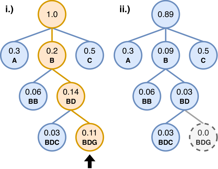
Figure 1: Example of incremental sampling using a trie. Nodes represent partial sequences (here, letters) and contain their total probabilities. i.) The sequence ’BDG’ is sampled from the model, and we subtract its total probability from its ancestors. ii.) Updated trie after erasing ’BDG’.

In this section, we describe our main contribution, a way to sample sequences without replacement in multiple rounds as described in Shi et al. (2020), coupled with a policy update after each round. We begin with a recall of Stochastic Beam Search (Kool et al., 2019c) using the Gumbel Top-k trick (Gumbel, 1954; Yellott Jr., 1977; Vieira, 2014), followed by a description of how to split the process into multiple rounds using an augmented trie, as described by Shi et al. (2020). We then describe how to combine the trie with a policy update. In the following, we use the term "beam search" to refer to the variant of beam search common in natural language processing (NLP), where nodes in the trie correspond to partial sequences, and a beam search of width $k$ keeps the top $k$ most probable sequences at each step, ranked by the total log-probability $\log\pi(\bm{a}_{1:t})=\sum_{t^{\prime}=1}^{t}\log\pi(a_{t^{\prime}}|\bm{a}_{1:t^{\prime}-1})$.

4.1 Preliminaries

Stochastic Beam Search

SBS is a modification of beam search that uses the Gumbel Top-k trick to sample sequences without replacement by using Gumbel perturbed log-probabilities. SBS starts at the root node (i.e., an empty sequence) $\bm{a}_{1:0}$ and sets the root perturbed log-probability $G_{\bm{a}_{1:0}}:=0$. Now, at any step during the beam search, let $\bm{a}_{1:t}$ be a partial sequence with score $G_{\bm{a}_{1:t}}$. Then, for a direct child $\bm{a}_{1:t+1}\in\text{Children}(\bm{a}_{1:t})$, we sample the perturbed log-probability $G_{\bm{a}_{1:t+1}}\sim\text{Gumbel}(\log\pi(\bm{a}_{1:t+1}))$ from a Gumbel distribution with location $\log\pi(\bm{a}_{1:t+1})$ under the condition that $\max_{\bm{a}_{1:t+1}\in\text{Children}(\bm{a}_{1:t})}G_{\bm{a}_{1:t+1}}=G_{\bm{a}_{1:t}}$, and use the $G_{\bm{a}_{1:t+1}}$’s as the scores for the beam search. By requiring that the maximum of the perturbed log-probabilities of sibling nodes must be equal to their parent’s, sampled Gumbel noise is consistently propagated down the subtree. Kool et al. show that this modified beam search is equivalent to sampling $k$ sequences without replacement from the sequence model $\pi$, yielding diverse but high-quality sequences. Since SBS performs the expansion of the beam as in regular deterministic beam search, it can be parallelized in the same way. We provide a detailed summary of the underlying theory in Appendix A.

Incremental Sampling Without Replacement

Shi et al. (2020) present an incremental view on sampling sequences without replacement that can draw one sequence after another. They suggest maintaining an augmented trie structure that grows with the sampling process, where nodes correspond to partial sequences as in beam search. Starting from the root node (representing an empty sequence), a single leaf node $\bm{a}_{1:T}$ (representing a complete sequence) is sampled from the sequence model $\pi$. Then the total probability of $\pi(\bm{a}_{1:T})$ is recursively subtracted from the probability of the leaf and its ancestors (which correspond to all partial sequences $\bm{a}_{1:0},\bm{a}_{1:1},\dots,\bm{a}_{1:T}$). After renormalization of the probabilities, the trie represents a sequence model from which $\bm{a}_{1:T}$ has been removed, and re-sampling from this updated trie is equivalent to sampling from the model conditioned on the fact that $\bm{a}_{1:T}$ cannot be selected (see Figure 1). The incremental nature of the process has the advantage that we can sample continuously without replacement, stopping only when some condition is met. To further exploit the parallelism advantages of SBS, Shi et al. (2020) suggest combining SBS with their method: Instead of drawing just one sequence, we use the same trie for SBS and draw a batch of $k$ samples in parallel. Then, the recursive probability update is done for all $k$ sequences. This allows us to sample batches in rounds, e.g., with a beam width of $k$ and $n$ rounds, we sample $k\cdot n$ sequences without replacement. Note that although we must maintain a trie structure, each round of SBS maintains the constant memory requirements of a beam search of width $k$.

4.2 Sampling with Gumbeldore

In the following, let $x\sim\mathcal{X}$ be a problem instance, and let $k$ be the beam width for SBS and $n$ the number of rounds. For sampling from a policy $\pi$ in Algorithm 1 above, we use the batch-wise sampling in $n$ rounds to draw $k\cdot n$ sequences without replacement. Suppose that in the first round we sample complete trajectories $\bm{a}_{1:T}^{(1)},\dots,\bm{a}_{1:T}^{(k)}$ with SBS. The question arises since we already have $k$ complete trajectories, and thus their evaluations $f_{x}(\bm{a}_{1:T}^{(i)})\in\mathbb{R}$, can we get information about their quality and use it in the next round of SBS? Intuitively, for the next round of sampling, we would like to move in the trie from $\pi$ to a policy $\pi^{\prime}$ that puts more emphasis on tokens that have led to ’good’ solutions and less emphasis on tokens that have led to ’not-so-good’ solutions.

4.2.1 Trie update

Theoretical policy improvement

To theoretically motivate our approach, consider any complete trajectory $\bm{a}_{1:T}=(a_{1},\dots,a_{T})$ and a policy $\pi$. We can move to an improved policy $\pi^{\prime}$ by shifting the unnormalized log-probability (’logit’) of the intermediate tokens of $\bm{a}_{1:T}$ by their individual advantage. That is, for $i\in\{1,\dots,T\}$, we set

$$\begin{split}\text{logit }\pi^{\prime}(a_{i}|\bm{a}_{1:i-1}):=&\log\pi(a_{i}|\bm{a}_{1:i-1})+\\ &\sigma\cdot\left(\underbrace{\mathbb{E}_{\bm{a}^{\prime}_{1:T}\sim\pi(\cdot|\bm{a}_{1:i})}\left[f_{x}(\bm{a}^{\prime}_{1:T})\right]-\mathbb{E}_{\bm{a}^{\prime}_{1:T}\sim\pi(\cdot|\bm{a}_{1:i-1})}\left[f_{x}(\bm{a}^{\prime}_{1:T})\right]}_{\text{advantage of token $a_{i}$}}\right).\end{split}$$ (1)

Here, $\sigma>0$ is a predefined size of the update step, and $\bm{a}^{\prime}_{1:T}\sim\pi(\cdot|\bm{a}_{1:i})$ denotes a complete sequence $\bm{a}^{\prime}_{1:T}=(a^{\prime}_{1},\dots,a^{\prime}_{T})$ drawn from $\pi$ where $a^{\prime}_{j}=a_{j}$ for all $j\in\{1,\dots,i\}$. Informally, (1) increases the probability of tokens that have a better expected outcome than their parent and decreases it otherwise. Formally, (1) yields a policy improvement, i.e., we get

$$\mathbb{E}_{\bm{a}_{1:T}\sim\pi^{\prime}}\left[f_{x}(\bm{a}_{1:T})\right]\geq\mathbb{E}_{\bm{a}_{1:T}\sim\pi}\left[f_{x}(\bm{a}_{1:T})\right],$$ (2)

and we provide a proof of this in Appendix B.

Practical policy update

Let $\bm{a}^{(1)},\dots,\bm{a}^{(k)}$ be $k$ complete trajectories sampled with SBS, which we assume to be ordered by their perturbed log-probabilities $G_{\bm{a}^{(1)}}\geq\cdots\geq G_{\bm{a}^{(k)}}$. We have omitted $1:T$ in the subscript for ease of notation. Motivated by its provable improvement, we would like to apply (1) to all $\bm{a}^{(i)}$, but the update relies on our ability to estimate the corresponding expectations. Kool et al. (2019c) present an unbiased estimator of the objective function expectation of the sequence model:

$$\mathbb{E}_{\bm{a}_{1:T}\sim\pi}\left[f_{x}(\bm{a}_{1:T})\right]\approx\sum_{i=1}^{k-1}w_{\bm{a}^{(k)}}(\bm{a}^{(i)})f_{x}(\bm{a}^{(i)}),\text{ where }w_{\bm{a}^{(k)}}(\bm{a}^{(i)})=\frac{\pi(\bm{a}^{(i)})}{q_{\bm{a}^{(k)}}(\bm{a}^{(i)})},$$ (3)

and $q_{\bm{a}^{(k)}}(\bm{a}^{(i)})=P(G_{\bm{a}^{(i)}}>G_{\bm{a}^{(k)}})$ is the probability that the $i$-th perturbed log-probability is greater than the $k$-th largest. In practice, the normalized variant (which is biased but consistent)

$$\mu(\bm{a}^{(1)},\dots,\bm{a}^{(k)}):=\frac{\sum_{i=1}^{k-1}w_{\bm{a}^{(k)}}(\bm{a}^{(i)})f_{x}(\bm{a}^{(i)})}{\sum_{i=1}^{k-1}w_{\bm{a}^{(k)}}(\bm{a}^{(i)})}$$ (4)

is preferred to reduce variance. Note that (4) estimates the ’full’ expectation from an empty sequence. However, since in SBS, the maximum of the perturbed log-probabilities of sibling nodes is conditioned on their parent, we can also estimate the expectation starting from other partial sequences: For any sequence $\bm{b}_{1:j}$ of length $j$, let $S(\bm{b}_{1:j}):=\{\bm{a}^{(m_{1})},\dots,\bm{a}^{(m_{l})}\}\subseteq\{\bm{a}^{(1)},\dots,\bm{a}^{(k)}\}$ (again ordered by their perturbed log-probabilities) be the subset of all sampled sequences that share the subsequence $\bm{b}_{1:j}$. I.e., we have $\bm{b}_{1:j}=\bm{a}_{1:j}^{(m_{1})}=\cdots=\bm{a}_{1:j}^{(m_{l})}$. Then,

$$\mathbb{E}_{\bm{a}_{1:T}\sim\pi(\cdot|\bm{b}_{1:j})}\left[f_{x}(\bm{a}_{1:T})\right]\approx\mu(\bm{a}^{(m_{1})},\dots,\bm{a}^{(m_{l})})$$ (5)

estimates the expectation of the objective function given $\bm{b}_{1:j}$. While we can use this approach to apply (1) to the logits of any $\bm{a}^{(i)}$, it has a major drawback: Depending on the length $T$ of the problem, the beam width $k$, and the confidence of $\pi$, in practice the sampled sequences will rarely share a long subsequence, which makes it hard to properly estimate the expectation of nodes deep in the trie.

So we take a practical approach and only use the ’global’ advantage $f_{x}(\bm{a}^{i})-\mu(\bm{a}^{(1)},\dots,\bm{a}^{(k)})$, which we propagate up the trie at the same time as we mark $\bm{a}^{(i)}$ as sampled. Overall, the trie update after each round of sampling can then be summarized as follows: For all $i\in\{1,\dots,k\}$, we compute the global advantage $A_{\bm{a}^{(i)}}:=f_{x}(\bm{a}^{(i)})-\mu(\bm{a}^{(1)},\dots,\bm{a}^{(k)})$, and update the logit for each $j\in\{1,\dots,T\}$ via

$$\text{logit }\pi^{\prime}(a_{j}^{(i)}|\bm{a}_{1:j-1}^{(i)}):=\log\left(\pi(a_{j}^{(i)}|\bm{a}_{1:j-1}^{(i)})-\sum_{\bm{b}\in S(\bm{a}_{1:j}^{(i)})}\pi(\bm{b})\right)+\sigma\sum_{\bm{b}\in S(\bm{a}_{1:j}^{(i)})}A_{\bm{b}}.$$ (6)

We illustrate an example of the trie update after each round in Figure 2. We note that as all expectations are obtained via (4), the update (6) adds no significant computational overhead to the round-based SBS. When samling another $k$ sequences in the next round, we repeat the process.

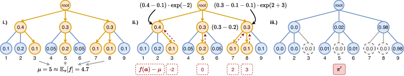
Figure 2: Example of update (6) with beam width $k=3$ and $\sigma=1$. Nodes represent partial sequences and their total probabilities; the numbers $\{1,\dots,9\}$ below the leaf nodes are their corresponding objective function evaluation. i.) We sample $k$ leaf nodes with SBS and obtain the objective function estimate $\mu$ with (4). ii.) We mark each leaf as sampled by removing its total probability from its ancestors. At the same time (equivalent to adding to the log-probability), we multiply the ancestors’ reduced probability by the exponential of the leaf’s advantage. iii.) Trie after normalization, corresponding to $\pi^{\prime}$.

Choice of step size $\sigma$

The update (6) scales the probabilities by $\exp(\sigma\sum A_{\bm{b}})$, so the role of the hyperparameter $\sigma$ is mainly to dampen the advantage. Since the magnitude of $\sum A_{\bm{b}}$ usually also changes as the model $\pi$ evolves, the choice of $\sigma$ is highly problem-dependent. In particular, one could think of, e.g., transforming the $A_{\bm{b}}$ by min-max normalization or changing $\sigma$ during training to optimize the behavior of the update. However, our experiments use the pure advantages and a constant, small problem-dependent $\sigma$ throughout the training process (see Section 5.3).

4.2.2 Growing nucleus

To further exploit the round-based sampling strategy, we truncate the conditional distributions $\pi(\cdot|\bm{a}_{1:t})$ using Top-$p$ (nucleus) sampling (Holtzman et al., 2020) at each beam expansion in SBS with varying $p$. If $n>1$ is the number of rounds, then we set $p$ for the $i$-th round with $1\leq i\leq n$ to $\displaystyle p=\left(1-\frac{i-1}{n-1}\right)\cdot p_{\text{min}}+\frac{i-1}{n-1}$. We start at a predefined $0<p_{\text{min}}<1$ and linearly increase $p$ to 1. The idea is that truncating the "unreliable tail" of $\pi(\cdot|\bm{a}_{1:t})$ with $p<1$ may be desirable in later stages of training to further exploit the model. However, if the model is unreliable, especially in the early stages, we want to consider the full distribution to encourage exploration. By gradually increasing $p$, we accommodate both cases, while the trie policy update helps keep good choices in the nucleus and pushes bad ones out. In practice, we start with $p_{\text{min}}=1$ and set $p_{\text{min}}=0.95$ after several epochs. When sampling at inference time, an even smaller $p_{\text{min}}$ can improve the results (cf. Appendix C.2). During training, however, we found that using $p_{\text{min}}<0.9$ leads to the model converging prematurely as it only learns to amplify its decisions.

We summarize the complete sampling strategy in Algorithm 2.

Input: $x\sim\mathcal{X}$: problem instance; $f=f_{x}$: objective function; $\pi$: policy

Input: $k$: beam width for SBS; $n$: number of rounds

Input: $\sigma$: policy update step size; $p_{\text{min}}$: minimum nucleus size

Output: Sampled sequence with highest $f$

1 $\textsc{Sampled}\leftarrow\emptyset$

2 for $i=1,\dots,n$ do

3       $p\leftarrow(1-\frac{i-1}{n-1})\cdot p_{\text{min}}+\frac{i-1}{n-1}$

4       $\bm{a}_{1:T}^{(1)},\dots,\bm{a}_{1:T}^{(k)}\leftarrow$ SBS with $\pi$, beam width $k$ and nucleus $p$

5       $\textsc{Sampled}\leftarrow\textsc{Sampled}\cup\{\bm{a}_{1:T}^{(1)},\dots,\bm{a}_{1:T}^{(k)}\}$

6       Obtain $\mathbb{E}_{\pi}[f]$ estimate $\mu\leftarrow\mu(\bm{a}^{(1)},\dots,\bm{a}^{(k)})$ via (4)

7       $\pi^{\prime}\leftarrow\pi$

8       for $j=1,\dots,k$ do

9             for $m=1,\dots,T$ do

                   $S\leftarrow S(\bm{a}_{1:m}^{(j)})\subseteq\{\bm{a}_{1:T}^{(1)},\dots,\bm{a}_{1:T}^{(k)}\}$

                    $\triangleright$ sequences with same first $m$ tokens

10                   $\text{logit }\pi^{\prime}(a_{m}^{(j)}|\bm{a}_{1:m-1}^{(j)})\leftarrow\log\left(\pi(a_{m}^{(j)}|\bm{a}_{1:m-1}^{(j)})-\sum_{\bm{b}\in S}\pi(\bm{b})\right)+\sigma\sum_{\bm{b}\in S}(f(\bm{b})-\mu)$

11                  

12            

13      

Return $\operatorname*{arg\,max}_{\bm{a}\in\textsc{Sampled}}f(\bm{a})$

Algorithm 2 Sampling with Gumbeldore (GD)

5 Experimental Evaluation

We are pursuing two experimental goals: First, we want to evaluate the effectiveness of our method within the entire training cycle of the self-improvement strategy (see Algorithm 1), and we test it on three CO problems with different underlying network architectures: the two-dimensional Euclidean TSP, the CVRP, and the standard JSSP. Second, as the training relies on the effectiveness of the solution sampling, we want to assess the solution quality of our sampling strategy (especially with a low number of samples). We take various network checkpoints of all three problems and compare different sampling techniques to our proposed method.

5.1 Routing problems

We consider two prevalent routing problems, the two-dimensional Euclidean TSP and CVRP, where the constructive approach builds a tour by picking one node after another. For both problems, we reimplement the transformer-based architecture from the recent Bisimulation Quotienting (BQ) method (Drakulic et al., 2023). This model has nine layers that process the remaining nodes at each step. In the original work, due to its size, BQ is trained on expert trajectories from solvers with $N=100$ nodes. The authors report excellent results on the training distribution and superior generalization on larger graphs with $N\in\{200,500,1000\}$ nodes. We train the network on instances with 100 nodes in the same way and additionally with our self-improvement method, where we sample trajectories with Gumbeldore (SI GD). The setup is briefly outlined below. For implementation details and hyperparameters, please refer to Appendix D.2 and D.3. Furthermore, the ’Light Encoder Heavy Decoder’ (LEHD) by (Luo et al., 2023) follows a similar paradigm to BQ. Apart from supervised learning, they show a problem-specific way to learn on the TSP without any labeled data. We discuss this method in Appendix C.1 and demonstrate that SI GD outperforms it.

Datasets and supervised training

Training (for supervised learning), validation, and test data are generated in the standard way of previous work (Kool et al., 2019b) by uniformly sampling $N$ points from the two-dimensional unit square. The training dataset consists of one million randomly generated instances with $N=100$ nodes for TSP. The validation and test sets (also $N=100$) include 10,000 instances each. The test set is the same widely used dataset generated by Kool et al. (2019b). For $N\in\{200,500,1000\}$, we use a test set of 128 instances identical to Drakulic et al. (2023). For supervised training and to compute optimality gaps, we obtain optimal solutions for the generated instances with the Concorde solver (Applegate et al., 2006). For the CVRP, the datasets have the same number of instances, and we use the same sets as in Luo et al. (2023), where solutions come from HGS (Vidal, 2022). The vehicle capacities for 100, 200, 500, and 1000 nodes are 50, 80, 100, and 250, respectively. The supervised model is trained by imitation of the expert solutions using a cross-entropy loss. We sample 1000 batches of 1024 sub-paths in each epoch, following Drakulic et al. (2023). The model is trained until we have yet to observe any improvement on the validation set for 100 epochs (in total $\sim$4.5k epochs for TSP and $\sim$1.3k for CVRP). We note that we can reproduce (up to fluctuations) the results from the original work.

Gumbeldore training

We generate to 1,000 random instances in each epoch for SI GD. Per instance, we sample 128 solutions in $n=4$ rounds with a beam width of $k=32$. For the TSP, we set the constant $\sigma$ to scale the advantages to $\sigma=0.3$, and for CVRP to $\sigma=3$. We refer to Appendix D.1 for how we obtained these values. For both problems, we start with $p_{\text{min}}=1$ (no nucleus sampling) and set $p_{\text{min}}=0.95$ after 500 epochs. Training on the generated data is performed in the same supervised way (in total $\sim$2.2k epochs for TSP and $\sim$2.7k for CVRP). Interestingly, SI GD takes fewer epochs on the TSP and more on the CVRP than SL, confirming that it is much harder to learn heuristics from scratch for the CVRP. Our method cannot access optimality information, so we compare model checkpoints by their average tour length on the validation set.

Inference and baselines

All evaluations are performed with the model trained on $N=100$. We are mainly interested in how the self-improving model performs compared to its supervised counterpart (BQ SL) and thus focus on greedy results. We also report the results using a beam search of width 16 by Drakulic et al. (2023) for coherence. We also list the results (with a beam search of width 1024) of the Attention Model (AM) (Kool et al., 2019b), which was trained with self-critical REINFORCE. We also report the results for POMO (Kwon et al., 2020) with its best inference technique (corresponding to $8N$ diversified solutions per instance of size $N$). POMO is considered the current state-of-the-art method of learning constructive heuristics from scratch. POMO performs impressively on the training distribution but has difficulties generalizing to larger instances. As our architectural setup is identical to BQ, we refer to the original work by (Drakulic et al., 2023) for comparison with various other methods.

Table 1: Results for TSP and CVRP. Gaps are computed w.r.t Concorde (Applegate et al., 2006) for TSP and HGS (Vidal, 2022) for CVRP.

Method	Test (10k inst.)		Generalization (128 instances)
	TSP $N=100$		TSP $N=200$		TSP $N=500$		TSP $N=1000$
	Gap	Time	Gap	Time	Gap	Time	Gap	Time
AM, beam 1024	2.49%	5m	6.18%	15s	17.98%	2m	29.75%	7m
POMO, augx8	0.14%	15s	1.57%	2s	20.18%	16s	40.60%	3m
BQ SL, greedy	0.40%	30s	0.60%	3s	0.98%	16s	1.72%	32s
BQ SL, beam 16	0.02%	8m	0.09%	30s	0.43%	4m	0.91%	10m
BQ SI GD (ours), greedy	0.41%	30s	0.64%	3s	1.12%	16s	2.11%	32s
BQ SI GD (ours), beam 16	0.02%	8m	0.10%	30s	0.46%	4m	1.01%	10m
	CVRP $N=100$		CVRP $N=200$		CVRP $N=500$		CVRP $N=1000$
	Gap	Time	Gap	Time	Gap	Time	Gap	Time
AM, beam 1024	4.20%	10m	8.18%	24s	18.01%	3m	87.56%	12m
POMO, augx8	0.69%	25s	4.87%	3s	19.90%	24s	128.89%	4m
BQ SL, greedy	3.03%	0s	2.63%	4s	3.75%	22s	5.30%	48s
BQ SL, beam 16	1.22%	13m	1.15%	1m	1.93%	6m	2.49%	15m
BQ SI GD (ours), greedy	3.26%	50s	3.05%	4s	3.89%	22s	8.33%	48s
BQ SI GD (ours), beam 16	1.72%	13m	1.58%	1m	2.32%	6m	5.57%	15m

Results

Table 1 summarizes the optimality gaps. For the TSP, our proposed method achieves results on par with its SL counterpart on the training distribution $N=100$ and shows similarly strong generalization capabilities. For the CVRP, while the results are close to SL on $N=100$, the generalization difference becomes larger as $N$ grows, with, for example, a difference of $\sim 3\%$ on $N=1000$. We note that generalizing to larger instances means not only larger $N$ but also unseen vehicle capacities. Drakulic et al. (2023) analyze that the final performance of the model strongly depends on how an expert solution sorts the subtours. In particular, the model favors learning from solutions where the vehicle starts with subtours with the smallest remaining vehicle capacity at the end of the subtour (usually 0). Since we cannot guarantee during learning in our SI procedure that the vehicle is nearly optimally utilized in the subtours, we assume that this makes it more difficult for the model to generalize to unknown capacities. Nevertheless, the SI GD generalization results for CVRP still show the same strong dynamics as those of BQ SL, trained without any labeled data. This makes our method a promising alternative to RL-based policy gradient methods, especially due to its simplicity.

5.2 Job-Shop Scheduling Problem

In a JSSP instance of size $J\times M$, we are given $J$ jobs consisting of $M$ operations. Each job’s operations must be processed in order (called a precedence constraint), and each operation runs on exactly one of $M$ machines for a given processing time (i.e., there is a bijection between a job’s set of operations and the set of machines). The goal is to find a schedule that processes all job operations without violating the job’s precedence constraints and has a minimum makespan (i.e., the completion time of the last operation). In our required sequential language, we represent a feasible solution, i.e., a schedule that satisfies all precedence constraints, as a sequence of jobs, where each occurrence of a job means scheduling the next unscheduled operation of the job at the earliest possible time. In particular, the model predicts a probability distribution over all unfinished jobs at each step of constructing a solution.

Table 2: JSSP results on the Taillard benchmark set. ’GD $32\times 4$’ refers to using GD sampling with four rounds of beam width 32, using $p_{\text{min}}=0.8$. For GD $32\times 4$ and SBS 16, we report the mean across five repetitions.

	$15\times 15$		$20\times 15$		$20\times 20$		$30\times 15$		$30\times 20$		$50\times 15$		$50\times 20$		$100\times 20$
Method	Gap	Time	Gap	Time	Gap	Time	Gap	Time	Gap	Time	Gap	Time	Gap	Time	Gap	Time
L2D, greedy	26.0%	0s	30.0%	0s	31.6%	1s	33.0%	1s	33.6%	2s	22.4%	2s	26.5%	4s	13.6%	25s
ScheduleNet, greedy	15.3%	3s	19.4%	6s	17.2%	11s	19.1%	15s	23.7%	25s	13.9%	50s	13.5%	1.6m	6.7%	7m
SPN, greedy	13.8%	0s	15.0%	0s	15.2%	0s	17.1%	0s	18.5%	1s	10.1%	1s	11.6%	1s	5.9%	2s
L2S, 500 steps	9.3%	9s	11.6%	10s	12.4%	11s	14.7%	12s	17.5%	14s	11.0%	16s	13.0%	23s	7.9%	50s
SI GD (ours), greedy	9.6%	1s	9.9%	1s	11.1%	1s	9.5%	1s	13.8%	2s	2.7%	2s	6.7%	3s	1.7%	28s
L2S, 5000 steps	6.2%	1.5m	8.3%	1.7m	9.0%	1.9m	9.0%	2m	12.6%	2.4m	4.6%	2.8m	6.5%	3.8m	3.0%	8.4m
SI GD (ours), beam 16	10.1%	2s	9.8%	2s	10.4%	4s	8.5%	5s	12.3%	10s	2.6%	18s	7.7%	40s	1.3%	1.5m
SI GD, SBS 16, $p=0.8$	6.0%	2s	6.6%	2s	8.9%	4s	7.4%	5s	10.5%	10s	1.7%	18s	5.0%	40s	0.7%	1.5m
SI GD, GD $32\times 4$	5.0%	4s	5.6%	10s	7.0%	30s	5.8%	36s	9.2%	1.3m	1.1%	2.4m	4.3%	3.5m	0.4%	9m

Model

We propose a novel pure transformer-based architecture inspired by the BQ principle Drakulic et al. (2023) to train a model with our SI GD method. We consider a JSSP instance as an unordered sequence of operations with positional information for operations belonging to the same job. We mask already scheduled operations at each construction step and process the sequence through a simple stack of pairs of attention layers. In each pair, we mask operations so that i.) in the first layer, only operations that belong to the same job can attend to each other, and ii.) in the second layer, only operations that need to run on the same machine can attend to each other. We describe the architecture in detail in Appendix D.4. To balance inference speed and model expressiveness, we settle on a latent dimension of 64, three pairs of attention layers with eight heads, and a feed-forward dimension of 256.

Datasets

All random instances are generated in the standard manner of Taillard (1993) with integer processing times in $[1,99]$. Since we train our model with SI GD, we only pre-generate a validation set of 100 instances of size $20\times 20$. We test our model on the well-known Taillard benchmark dataset (Taillard, 1993), computing optimality gaps to the best-known upper bounds.

Gumbeldore training

We train our model for 100 epochs, where for each epoch, we randomly choose a size from $\{15\times 10,15\times 15,15\times 20\}$ and sample 512 instances of the chosen size. We generate 128 solutions for each instance in 4 rounds of beam width 32 with $\sigma=0.05$. After 50 epochs, we set $p_{\text{min}}=0.95$. Similar to the routing problems, we sample 1,000 incomplete schedules (i.e., a partial sequence of jobs) of size 512 from the generated training data. We train the model to predict the next job to choose using a cross-entropy loss. Please see Appendix D.4 for more details.

Inference and baselines

We test the model performance in four different ways: i.) unrolling the policy greedily, ii.) with a beam search of width 16, iii.) SBS of beam width 16 with a constant nucleus of $p=0.8$ and iv.) sampling with GD to evaluate the efficiency of GD as an inference technique. We compare our approach with L2D (Zhang et al., 2020), an RL single-agent method, and ScheduleNet (Park et al., 2022), an RL multi-agent method. Both methods represent a JSSP instance as a disjunctive graph and train Graph Neural Networks (GNN) with (variants of) PPO (Schulman et al., 2017). We also compare to the variants with 500 and 5,000 steps of L2S (Zhang et al., 2024), a strong GNN-guided improvement method that transitions between complete solutions in each step. Finally, we list the recent SPN (Corsini et al., 2024) results. This concurrent work trains a Graph Attention Network in a self-improving manner on sampled solutions (we refer to Appendix E for a methodological comparison). As noted in most previous work on neural CO, a fair comparison of inference times is challenging, as they depend on the implementation (especially using deep learning frameworks) by orders of magnitude. In particular, we report the time required to solve the instances of a given size (allowing parallelization) but compare the respective methods based on their inference type (e.g., treating greedy methods as equally computationally intensive).

Results

We collect the results in Table 2. In the greedy setting, we outperform all three constructive methods, L2D, ScheduleNet, and SPN, by a wide margin and obtain smaller gaps than L2S with 500 improvement steps in all but one case. The quadratic complexity of our architecture becomes noticeable for $100\times 20$. When allowing for longer inference times, we compare our method only to the strongest method, L2S with 5,000 improvement steps. We note that our method does not always improve with beam search, with some results even worse than greedy. That sequences with high overall probability do not necessarily mean high quality is a ubiquitous effect in NLP (Holtzman et al., 2020), showing that the model is not as confident as for the routing problems. Thus, we sample with SBS and a constant nucleus of $p=0.8$. This maintains short inference times but outperforms L2S across all problem sizes. We can further improve the results by sampling with GD in multiple rounds (with $p_{\text{min}}=0.8$) and using our policy update. For more results and comparisons when using GD at inference time, see Appendix C.2.

5.3 Sampling performance

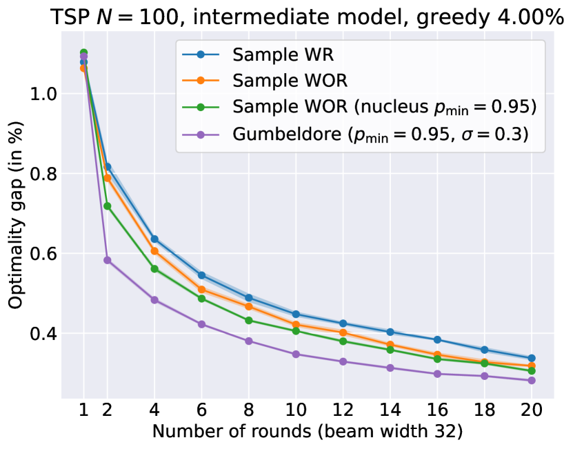
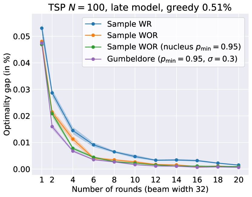
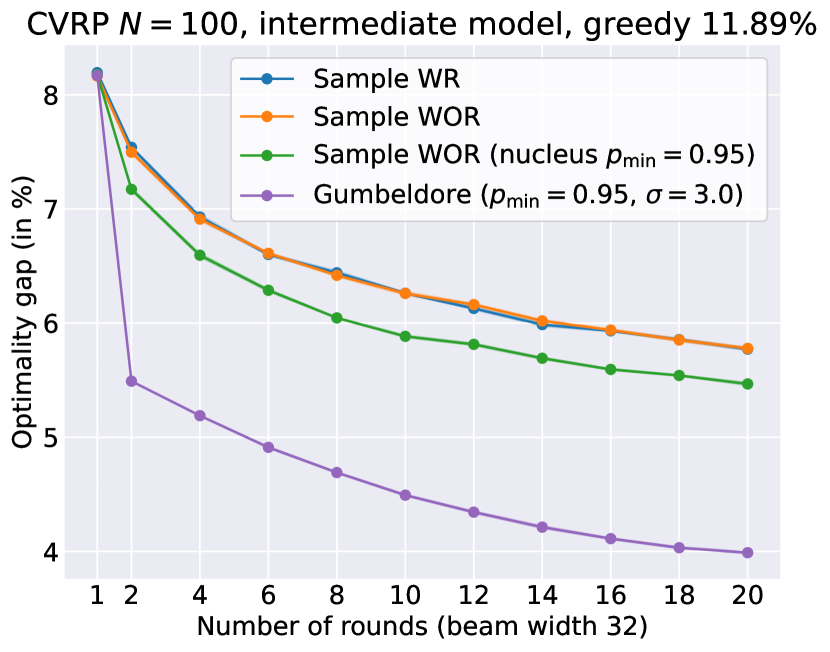
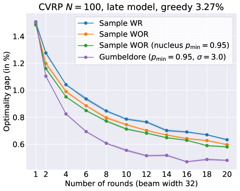
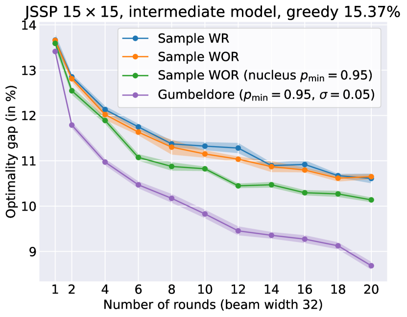
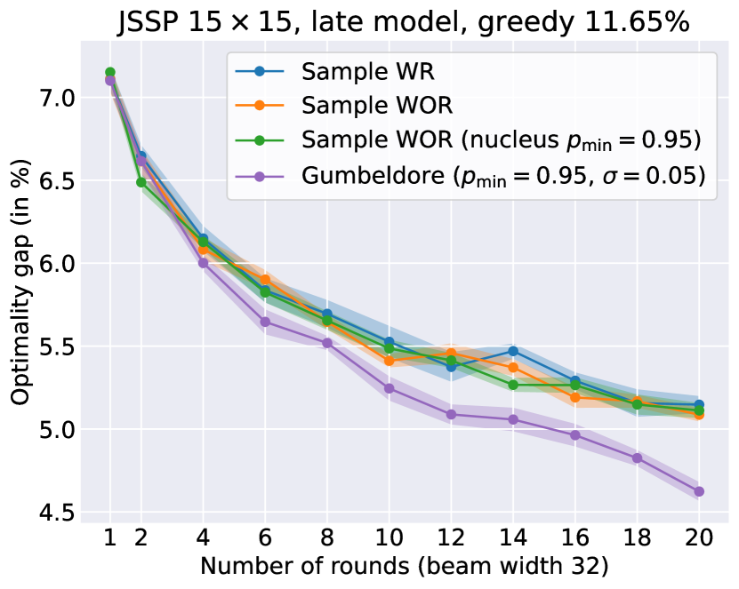
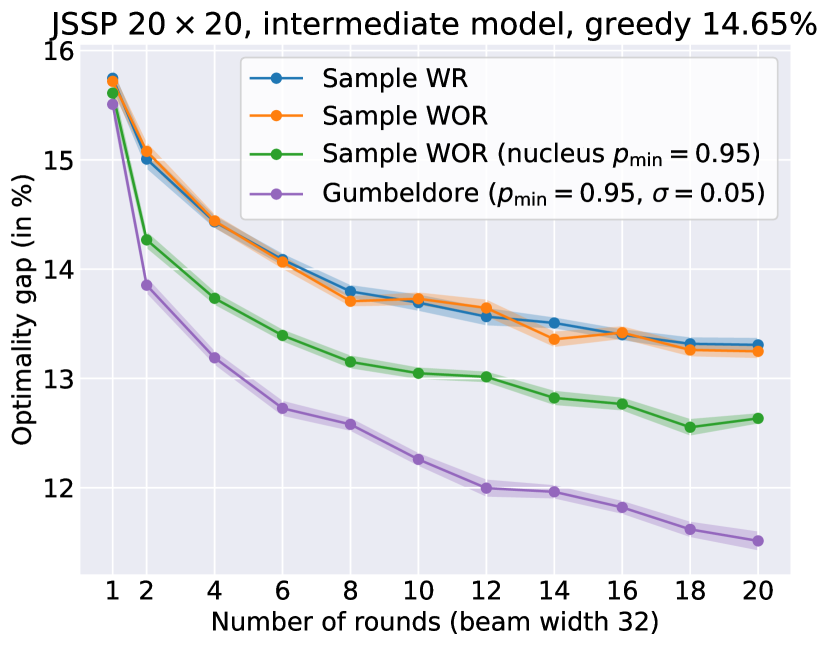
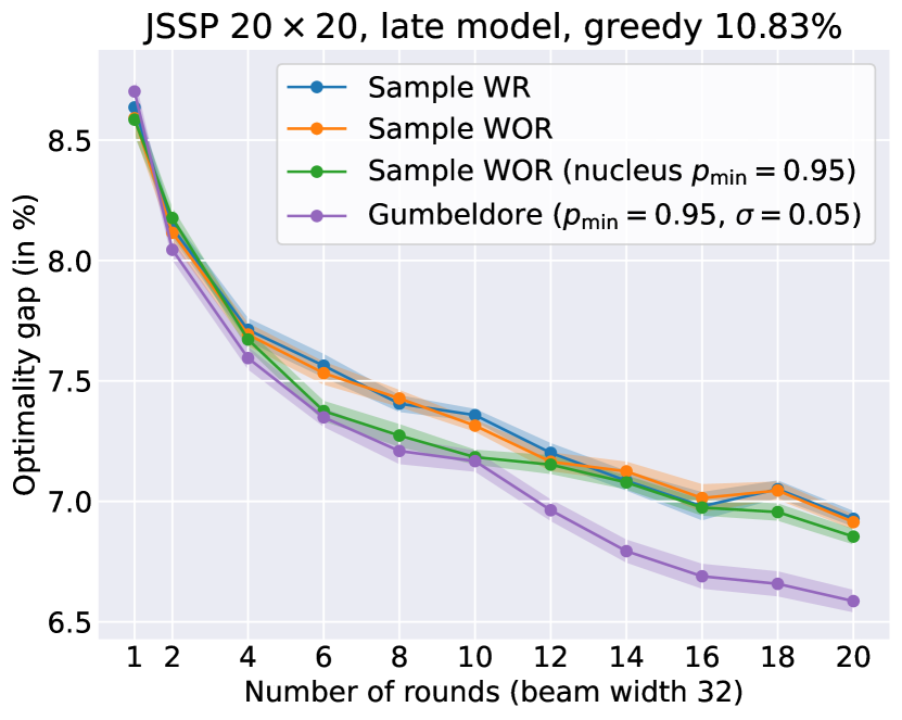
Figure 3: Sampling results for different training checkpoints, with the corresponding greedy performance of the model. For Sample WR, we sample $32\cdot n$ sequences with replacement, where $n$ is the number of rounds. For TSP and CVRP, each data point corresponds to the average best solution across 100 instances. For JSSP, we evaluate the Taillard instances of the corresponding size. Sampling for each data point is repeated 20 times; shades denote standard errors.

We analyze the performance of GD as a sampling technique, especially when sampling only a small number of sequences. For this, we take the model weights from two checkpoints during training: One late in training, when the model has almost converged, and an intermediate one, when the model shows a fair greedy performance but still has much room for improvement. Taking a checkpoint very early in training carries limited information, as the performance still depends strongly on weight initialization, and any sampling method with high exploration leads to substantial improvement. We then sample up to 640 sequences with an SBS beam width of 32 in up to $n=20$ rounds (for sampling with replacement, we sample the equivalent number of $32\cdot n$ sequences) and compare the optimality gap of the best sequences found. In Figure 3, we plot the results using our proposed method (’Gumbeldore’) and for sampling with (’Sample WR’) and without replacement (’Sample WOR’). To better understand the impact of the growing nucleus in Section 4.2.2, we also show the results for sampling without replacement with the growing nucleus, but without the policy update (6) (’Sample WOR (nucleus)’). We note that applying only one round of Sample WOR (nucleus) or GD is identical to Sample WOR by design. We use the same values for $p_{\text{min}}$ and $\sigma$ as during training.

In line with Shi et al. (2020), we observe that sampling WOR yields a consistent but slight improvement over WR for the routing problems but is almost unobservable for JSSP, which has a much longer sequence length (225 for $15\times 15$ and 400 for $20\times 20$). Generally, allowing different nucleus sizes can significantly improve the intermediate models while giving enough room for exploration. Further updating the policy between rounds with GD has a strong impact, especially on the intermediate models. For example, with only four rounds, we obtain an absolute improvement over Sample WOR of approx. 2% for CVRP and >1% for JSSP $20\times 20$ and reach an optimality gap with only 128 samples, which Sample WOR does not reach with 640 samples. While generally shrinking for only a few rounds, the relative improvement of GD is still significant in late models. In particular, GD consistently finds better solutions in late models when nucleus sampling only has limited influence. In Appendix C.3, we further illustrate the applicability of our method on a toy problem: we adapt our method for the board game Gomoku (Five in a Row) and evaluate how long it takes to consistently beat a deterministic expert bot.

6 Limitations and future work

Adjusting the policy by the advantage requires choosing a step size $\sigma$, which must be tuned for the problem class. To keep the approach principled, we left the step size fixed throughout training; however, the advantages’ magnitude usually shrinks as training progresses. Hence, it might be advantageous to change $\sigma$ during training based on problem specifics or normalize the advantages as mentioned in Section 4.2.1. Our method requires keeping a search tree in memory instead of only one round of SBS, where we can discard all previous sequences after each step. However, keeping transitions in memory has benefits, such as only evaluating the policy when needed and thus reducing computation time during search.

7 Conclusion

In this work, we introduced an approach for training neural combinatorial optimization models that bridges supervised learning and reinforcement learning challenges. During training, GD finds good solutions with only a few samples, eliminating the need for expert annotations while reducing computational demands. This method simplifies the training process and shows promise for enhancing the efficiency of neural combinatorial optimization using larger architectures.

Appendix A Background on Stochastic Beam Search

This section briefly describes the Gumbel-Top-k trick and the essence of Stochastic Beams and Where to Find Them (Kool et al., 2019c).

A.1 The Gumbel-Top-k trick

We denote by $\text{Gumbel}(\mu)$ a Gumbel distribution with location $\mu\in\mathbb{R}$ and unit scale. The distribution $\text{Gumbel}(0)$ is the standard Gumbel distribution. Similarly to Kool et al. (2019c); Huijben et al. (2022), we write $G_{\mu}$ for a random variable following $\text{Gumbel}(\mu)$, and omit $\mu$ in the subscript in the case of standard location $\mu=0$. The Gumbel distribution is closed under scaling and shifting, in particular for a standard $G\sim\text{Gumbel}(0)$ we have $\mu+G\sim\text{Gumbel}(\mu)$.

Gumbel-Max and Gumbel-Top-k trick

The following is a condensed summary of the preliminaries in Kool et al. (2019c), with attribution to Gumbel (1954); Yellott Jr. (1977); Maddison et al. (2014); Vieira (2014). Consider a discrete distribution $\text{Categorical}(p_{1},\dots,p_{K})$ with $K$ categories and the probability $p_{i}$ of the $i$-th category. Let $\phi_{i}$ be unnormalized log-probabilities (logits) for $p_{i}$, i.e., $p_{i}\propto\exp\phi_{i}$. We can obtain a sample from this distribution by perturbing each logit with a standard Gumbel and choosing the largest element (’Gumbel-Max trick’): Let $G_{\phi_{i}}=\phi_{i}+G_{i}$ with $G_{i}\sim\text{Gumbel}(0)$, then $G_{\phi_{i}}\sim\text{Gumbel}(\phi_{i})$ by the shifting property and $\operatorname*{arg\,max}_{i}G_{\phi_{i}}\sim\text{Categorical}(p_{1},\dots,p_{K})$.

In general, for any subset $B\subseteq\{1,\dots,K\}$ we have

$$\max_{i\in B}G_{\phi_{i}}\sim\text{Gumbel}\left(\log\sum_{j\in B}\exp\left(\phi_{j}\right)\right),\text{ and}$$ (7)

$$\operatorname*{arg\,max}_{i\in B}G_{\phi_{i}}\sim\text{Categorical}\left(\frac{\exp\left(\phi_{i}\right)}{\sum_{j\in B}\exp\left(\phi_{j}\right)},i\in B\right),$$ (8)

with $\max$ and $\operatorname*{arg\,max}$ being independent.

The Gumbel-Max trick can be generalized to drawing an ordered sample $(i_{1}^{*},\dots,i_{k}^{*})$ without replacement of size $k$ (’Gumbel-Top-$k$ trick’) by finding the indices of the top $k$ perturbed logits (denoted by $\operatorname*{arg\,top}k$):

$$i_{1}^{*},\dots,i_{k}^{*}=\operatorname*{arg\,top}_{i}k\ G_{\phi_{i}}.$$

A.2 Drawing samples without replacement from a sequence model

Beam search

Beam search is a low-memory, breadth-first tree search of limited beam width $k$. Given a policy $\pi$, the initial beam of a search from a root node (i.e., an empty sequence) with beam width $k$ consists of the top $k$ first tokens, ranked by their log-probability. Iteratively, at step $t$, each partial sequence in the beam expands its $k$ most probable tokens. The resulting expanded beam is again pruned down to $k$ by taking the top $k$ partial sequences according to their total log-probabilities $\log\pi(\bm{a}_{1:t})=\sum_{t^{\prime}=1}^{t}\log\pi(a_{t^{\prime}}|\bm{a}_{1:t^{\prime}-1})$, where $\bm{a}_{1:t}$ is any sequence in the expanded beam. Depending on the underlying factorized model, the final sequences found by beam search are often generic and lack variability (Vijayakumar et al., 2018).

Stochastic Beam Search

In Stochastic Beams and Where to Find Them (Kool et al., 2019c), Kool et al. apply the Gumbel-Top-k trick in an elegant way to sample sequences without replacement from a sequence model. Assuming that the full true is instantiated with all possible complete (leaf) sequences $\bm{a}_{1:T}^{(i)}$ with $i\in\{1,\dots,N\}$, one would sample distinct sequences with the Gumbel-Top-k trick by simply considering the perturbed log probabilities $G_{\phi_{i}}\sim\text{Gumbel}(\phi_{i})$, where $\phi_{i}=\log\pi(\bm{a}^{(i)}_{1:T})$. Of course, instantiating the full tree is computationally infeasible in practice. Instead, Kool et al. make the following crucial observation: Identify a node in the trie by the set $S$ of leaves in its corresponding subtree and denote the corresponding (partial) sequence by $\bm{a}^{S}$, with $\phi_{S}=\log\pi(\bm{a}^{S})$. Then

$$\max_{i\in S}G_{\phi_{i}}\overset{(\ref{eq:gumbel_max})}{\sim}\text{Gumbel}\left(\log\sum_{j\in S}\exp\phi_{j}\right)=\text{Gumbel}\left(\sum_{j\in S}\pi(\bm{a}^{(j)}_{1:T})\right)=\text{Gumbel}\left(\phi_{S}\right),$$ (9)

i.e., the maximum of the perturbed log probabilities of the leaf nodes in the subtree of $S$ follows a Gumbel distribution with location $\log\pi(\bm{a}^{S})$. Thus, instead of instantiating the full tree to sample $k$ sequences, we can equivalently sample top-down (Maddison et al., 2014) and perform a beam search of width $k$ over the perturbed log-probabilities by recursively propagating the Gumbel noise down the subtree according to (9): Let $\bm{a}^{S}$ be any partial sequence in the beam at any step of the beam search with perturbed log-probability $G_{\phi_{S}}$ (which we can set to zero for the root node). Then we sample $G_{\phi_{S^{\prime}}}$ for all direct children $S^{\prime}\in\text{Children}(S)$ under the condition that $\max_{S^{\prime}\in\text{Children}(S)}G_{\phi_{S^{\prime}}}=G_{\phi_{S}}$, and use $G_{\phi_{S^{\prime}}}$ as the scores for the beam search. We refer to the original paper by Kool et al. (2019c) for how to sample a set of Gumbels with a certain maximum.

Kool et al. (2019c) show on various language models that this simple procedure yields more diverse beam search results without sacrificing quality. From a sampling perspective, SBS can be seen as a principled way to randomize a beam search and construct stable unbiased estimators from a small number of sequences (Kool et al., 2019a; 2020).

Appendix B Policy Improvement Operation

We give a proof for the policy improvement obtained by Equation (1). The following lemma is part of the policy improvement proof for the updated action selection of Gumbel AlphaZero based on $Q$-value completion (Danihelka et al., 2022). For coherence, we formulate and prove it in our general setting, with attribution to Danihelka et al. (2022).

Lemma:

Consider a categorical distribution over the domain $\Omega=\{1,\dots,n\}$ with corresponding probabilities $\pi(i)$ for $i\in\Omega$. Consider a map $q\colon\Omega\to\mathbb{R}$, and let $j\in\Omega$. Let $\pi^{\prime}$ be the distribution obtained from $\pi$ by changing the unnormalized log-probability (’logit’) of $j$ to

$$\text{logit }\pi^{\prime}(j):=\log\pi(j)+q(j)-\mathbb{E}_{i\sim\pi}\left[q(i)\right].$$ (10)

Then, $\mathbb{E}_{i\sim\pi^{\prime}}\left[q(i)\right]\geq\mathbb{E}_{i\sim\pi}\left[q(i)\right]$.

Proof: We need to show that

$$\sum_{i\in\Omega}\pi^{\prime}(i)q(i)\geq\sum_{i\in\Omega}\pi(i)q(i).$$ (11)

Let $y=q(j)-\mathbb{E}_{i\sim\pi}\left[q(i)\right]$. If $\pi(j)=1$, then $y=0$, so $\pi^{\prime}=\pi$ and the claim is true. Hence, assume that $\pi(j)<1$. Note that for any $i\in\Omega\setminus\{j\}$, we have $\pi^{\prime}(i)=c\cdot\pi(i)$ with constant $c=\left(\sum_{i\in\Omega\setminus\{j\}}\pi(i)+\exp(y)\pi(j)\right)^{-1}$.

As $\sum_{i\in\Omega\setminus\{j\}}\pi(i)=1-\pi(j)$, we can rewrite $\mathbb{E}_{i\sim\pi}\left[q(i)\right]$ as

$$\mathbb{E}_{i\sim\pi}\left[q(i)\right]=\pi(j)q(j)+\sum_{i\in\Omega\setminus\{j\}}\pi(i)q(i) =\pi(j)q(j)+(1-\pi(j))\underbrace{\sum_{i\in\Omega\setminus\{j\}}\frac{\pi(i)q(i)}{\sum_{k\in\Omega\setminus\{j\}}\pi(k)q(k)}}_{=:\tilde{q}}$$ (12)

$$=\pi(j)q(j)+(1-\pi(j))\tilde{q}$$ (13)

$$=\pi(j)(q(j)-\tilde{q})+\tilde{q}.$$ (14)

Analogously, we get

$$\mathbb{E}_{i\sim\pi^{\prime}}\left[q(i)\right] =\pi^{\prime}(j)q(j)+(1-\pi^{\prime}(j))(1-\pi(j))\sum_{i\in\Omega\setminus\{j\}}\frac{c\pi(i)q(i)}{\sum_{k\in\Omega\setminus\{j\}}c\pi(k)q(k)}$$ (15)

$$=\pi^{\prime}(j)(q(j)-\tilde{q})+\tilde{q},$$ (16)

as the constant $c$ cancels out. In particular, equivalently to (11), we can show that

$$\pi^{\prime}(j)(q(j)-\tilde{q})\geq\pi(j)(q(j)-\tilde{q}).$$ (17)

By the policy update, we have $\pi^{\prime}(j)>\pi(j)\iff y>0$, so (17) follows if we can show that $y>0\iff(q(j)-\tilde{q})>0$. But this is true, as

$$y>0\iff q(j)>\mathbb{E}_{i\sim\pi}\left[q(i)\right] \iff q(j)>\pi(j)q(j)+(1-\pi(j))\tilde{q}$$ (18)

$$\iff(1-\pi(j))q(j)>(1-\pi(j))\tilde{q}$$ (19)

$$\overset{\pi(j)<1}{\iff}q(j)>\tilde{q}$$ (20)

$$\iff q(j)-\tilde{q}>0.$$ (21)

$\Box$

We can now prove the policy improvement over the entire sequence model.

Proposition:

Let $\pi$ be a policy, $\sigma>0$ and let $\bm{a}_{1:T}=(a_{1},\dots,a_{T})$ be a full sequence drawn from $\pi$. Let $\pi^{\prime}$ be the policy obtained from $\pi$ by changing the logit of $\pi^{\prime}(a_{i}|\bm{a}_{1:i-1})$ for all $i\in\{1,\dots,T\}$ to

$$\begin{split}\text{logit }\pi^{\prime}(a_{i}|\bm{a}_{1:i-1}):=&\log\pi(a_{i}|\bm{a}_{1:i-1})+\\ &\sigma\cdot\left(\mathbb{E}_{\bm{a}^{\prime}_{1:T}\sim\pi(\cdot|\bm{a}_{1:i})}\left[f_{x}(\bm{a}^{\prime}_{1:T})\right]-\mathbb{E}_{\bm{a}^{\prime}_{1:T}\sim\pi(\cdot|\bm{a}_{1:i-1})}\left[f_{x}(\bm{a}^{\prime}_{1:T})\right]\right).\end{split}$$ (22)

Then,

$$\mathbb{E}_{\bm{a}_{1:T}\sim\pi^{\prime}}\left[f_{x}(\bm{a}_{1:T})\right]\geq\mathbb{E}_{\bm{a}_{1:T}\sim\pi}\left[f_{x}(\bm{a}_{1:T})\right].$$ (23)

Proof: We omit $x$ in the subscript of $f$ to simplify the notation. As $\sigma$ only changes the magnitude of the step, we can assume without loss of generality that $\sigma=1$. We show the claim by induction on the length $T$.

For $T=1$, we have $\bm{a}_{1:T}=(a_{1})$, and the update reduces to

$$\text{logit }\pi^{\prime}(a_{1})=\log\pi(b)+f(a_{1})-\mathbb{E}_{a^{\prime}\sim\pi}\left[f(a^{\prime})\right].$$ (24)

Hence, the claim follows from the lemma above.

For the induction step for arbitrary $T$, we have

$$\mathbb{E}_{\bm{a}^{\prime}_{1:T}\sim\pi^{\prime}}\left[f(\bm{a}_{1:T})\right] =\sum_{\bm{a}^{\prime}_{1:T}}\pi^{\prime}(\bm{a}^{\prime}_{1:T})f(\bm{a}^{\prime}_{1:T})$$ (25)

$$=\sum_{a^{\prime}_{1}}\pi^{\prime}(a^{\prime}_{1})\mathbb{E}_{\bm{a}^{\prime}_{1:T}\sim\pi^{\prime}(\cdot|a^{\prime}_{1})}\left[f(\bm{a}^{\prime}_{1:T})\right]$$ (26)

$$\geq\sum_{a^{\prime}_{1}}\pi^{\prime}(a^{\prime}_{1})\mathbb{E}_{\bm{a}^{\prime}_{1:T}\sim\pi(\cdot|a^{\prime}_{1})}\left[f(\bm{a}^{\prime}_{1:T})\right],$$ (27)

where the last inequality follows from the induction hypothesis. But then, due to the form of the policy update (22), the lemma above can be applied again and we get

$$\sum_{a^{\prime}_{1}}\pi^{\prime}(a^{\prime}_{1})\mathbb{E}_{\bm{a}^{\prime}_{1:T}\sim\pi(\cdot|a^{\prime}_{1})}\left[f(\bm{a}^{\prime}_{1:T})\right] \geq\sum_{a^{\prime}_{1}}\pi(a^{\prime}_{1})\mathbb{E}_{\bm{a}^{\prime}_{1:T}\sim\pi(\cdot|a^{\prime}_{1})}\left[f(\bm{a}^{\prime}_{1:T})\right]$$ (28)

$$=\sum_{\bm{a}^{\prime}_{1:T}}\pi(\bm{a}^{\prime}_{1:T})f(\bm{a}^{\prime}_{1:T})$$ (29)

$$=\mathbb{E}_{\bm{a}^{\prime}_{1:T}\sim\pi}\left[f(\bm{a}^{\prime}_{1:T})\right],$$ (30)

what we wanted to show. $\Box$

Appendix C Extended experimental results

C.1 Comparison to self-improving training method for LEHD on TSP

Concurrently to Drakulic et al. (2023), Luo et al. (2023) propose the ’Light Encoder Heavy Decoder’ (LEHD) model for routing problems and also show promising generalization capabilities. The structure of LEHD is similar to BQ; however, while BQ only shares an affine embedding of the nodes across all time steps, LEHD encodes the nodes with a single attention layer. The decoder consists of six attention layers, and as in BQ, the model is trained to predict the next node of random subtours sampled from expert solutions. Luo et al. (2023) additionally present a training process on TSP that does not require solutions from solvers as follows:

• Train LEHD on TSP $N=20$ with self-critical REINFORCE for some time

• Generate a training set of 200,000 random instances of TSP $N=100$ and generate solutions for them with the current model.

• Sample subtours for each instance and randomly reconstruct (RRC) them to improve the solutions.

• Continue training of LEHD by supervised learning with the generated dataset.

In Table 3, we compare this approach (LEHD RL+RRC+SL) to their supervised approach and our method. We see that our simple training process based on sampling surpasses the relatively complicated RL + randomly reconstructed solutions approach and obtains results comparable to its supervised counterpart.

Table 3: Optimality gaps for TSP compared to LEHD with and without labeled data. For LEHD RL+RRC+SL, we take the results from the original paper, which are better than the ones we obtained with our implementation.

Method	Test	Generalization
	TSP $N=100$	TSP $N=200$	TSP $N=500$	TSP $N=1000$
LEHD SL, greedy	0.58%	0.95%	1.72%	3.34%
LEHD RL+RRC+SL, greedy	1.07%	1.45%	2.56%	4.52%
LEHD SI GD (ours), greedy	0.40%	0.72%	1.43%	3.30%

C.2 Gumbeldore at inference time

Table 4: Inference with Gumbeldore on the CVRP. For $N=100$, we only consider a test subset of 1000 instances. SBS and GD results are averaged over five repetitions. We use nucleus sampling with constant $p=0.8$ for SBS and GD, and keep $\sigma=3.0$ for GD.

Method	Test	Generalization
	$N=100$	$N=200$	$N=500$	$N=1000$
	Gap	Gap	Gap	Gap
Beam 128	1.16%	1.10%	1.72%	4.28%
Beam 256	1.00%	0.97%	1.60%	4.27%
Beam 512	0.86%	0.90%	1.40%	3.85%
SBS $32\times 4$	0.80%	1.07%	2.44%	6.04%
SBS $32\times 8$	0.65%	0.87%	2.34%	6.00%
SBS $64\times 8$	0.51%	0.73%	2.20%	5.80%
GD $32\times 4$	0.73%	1.03%	2.13%	5.25%
GD $32\times 8$	0.59%	0.76%	2.03%	5.12%
GD $64\times 8$	0.49%	0.56%	1.88%	4.76%

There is a plethora of work on how to exploit an already trained policy for neural CO, such as Simulation-Guided Beam Search Choo et al. (2022) or (Efficient) Active Search (Bello et al., 2016; Hottung et al., 2022) (cf. Section 2). Although we consider our sampling method mainly for training, in this section, we evaluate the performance during inference in the low sample regime. High exploration plays a subordinate role in this setting, so we use Top-$p$ sampling with a constant $p$ in all rounds. Table 4 shows inference results using the model trained with SI GD. We compare GD $k\times n$ with $n$ rounds and beam width $k$ to sampling without replacement (with Top-$p$) via round-based SBS $k\times n$ and to beam search with corresponding beam width. We see that both sampling methods outperform beam search on $N=100$ and $N=200$ but not on $N=500$ and $N=1000$. Furthermore, the policy update of GD leads to a consistent improvement over SBS. The CVRP results indicate that combining GD and deterministic beam search could result in a robust inference method. On the JSSP in Table 5, we observe the same improvement of GD over SBS. The margin, however, is not as wide as for intermediate models by Section 5.3. We omit the results for deterministic beam search on JSSP, as SBS supersedes them with nucleus sampling and a beam width of 16 (cf. Table 2).

Table 5: Inference with Gumbeldore on the JSSP. Results are averaged over five repetitions. In all cases, we use nucleus sampling with constant $p=0.8$, and keep $\sigma=0.05$ for GD.

	$15\times 15$	$20\times 15$	$20\times 20$	$30\times 15$	$30\times 20$	$50\times 15$	$50\times 20$	$100\times 20$
Method	Gap	Gap	Gap	Gap	Gap	Gap	Gap	Gap
SBS $32\times 4$	5.0%	5.7%	7.3%	6.1%	9.4%	1.1%	4.3%	0.4%
SBS $32\times 8$	4.7%	5.3%	7.0%	5.7%	9.0%	0.9%	4.0%	0.3%
SBS $64\times 8$	4.3%	5.3%	6.4%	5.2%	8.8%	0.9%	4.0%	0.3%
GD $32\times 4$	4.8%	5.6%	7.0%	5.8%	9.2%	1.1%	4.3%	0.4%
GD $32\times 8$	4.5%	5.3%	6.7%	5.3%	8.8%	0.9%	4.0%	0.3%
GD $64\times 8$	4.2%	4.8%	6.3%	5.0%	8.6%	0.8%	3.7%	0.2%

C.3 Gomoku: A toy problem

Played on a Go board, Gomoku is a game for two players who take turns placing their stones on the board, starting with black. The first player to have five stones in a row horizontally, vertically, or diagonally wins. We formulate the following problem: Given a deterministic expert bot playing black, how long does it take a greedy model playing white to learn from scratch to beat the opponent from all possible starting positions of black? Here, the model’s policy takes a board configuration and predicts a distribution over the next possible moves. We take the deterministic rule-based bot (’v1’), the Gomoku state representation, and the AlphaZero architecture for Go provided by the LightZero benchmark suite (Niu et al., 2023). In each epoch, we generate training data by sampling multiple trajectories using the current policy from all possible starting positions of black. Then, for each start position, we take from the sampled trajectories either a random trajectory where white wins or, if there is no win for white, a random trajectory where black wins. In the case of a draw, we take a random draw. The supervised training in each epoch then consists of learning the policy to predict the next move of the winner. After each epoch, we greedily unroll the policy for each starting position of black and count the number of times white wins. How many epochs does it take for white to win every time? The formulated problem is not standard, and board games are usually approached with self-play. Therefore, it is instead a tiny illustrative toy problem to further show the applicability of our method.

We play on a $9\times 9$ Go board. First, we let the model sample 320 sequences with replacement for each possible starting position and train the policy in each epoch on 100 batches of 32 pairs of the form (<board configuration>, <next move of winner>). Repeated ten times, the model takes an average of 60.2 epochs for white to consistently beat black.

For training with GD, we score a complete trajectory with its game result: 1 for a white win, -1 for a black win, and 0 for a draw. We also sample 320 sequences in 10 rounds with an SBS batch size of 32. We completely turn off nucleus sampling and use the game outcome as an advantage to propagate up the tree (equivalent to setting the expected outcome to a draw). Using a step size of $\sigma=5$, which heavily favors moves that lead to a win and punishing moves that lead to a lose, it takes an average of 47.7 epochs ($\sim 20\%$ faster than sampling with replacement) for white to greedily win all the time.

Appendix D Implementation and experimental details

Hardware and frameworks

Our code is developed in PyTorch (Paszke et al., 2019). Training and inference are performed for all experiments using two NVIDIA RTX A5000 with 24GB memory. As we do not need to collect gradients during sampling, we can easily parallelize solution sampling for different instances in each epoch. We spread it across 16 workers using ray.io.

D.1 Choice of Gumbeldore step size

We generally choose the step size $\sigma$ for the update in (6) as follows: We train the model using round-based SBS (i.e., with $\sigma=0$) for 20 epochs with four rounds of beam width 32. We then perform a grid search over $\sigma\in[0,5]$ on a small validation set.

D.2 Traveling Salesman Problem

D.2.1 Problem setup

In the Euclidean TSP with $N$ nodes in the unit square $[0,1]^{2}\subseteq\mathbb{R}^{2}$, a node permutation (i.e., a complete roundtrip, where all nodes are visited only once) with minimal edge weight should be found. A problem instance is defined by the two-dimensional coordinates of the $N$ nodes. The sequential problem asks for choosing one unvisited node at a time. The objective function to maximize evaluates a full tour by the negative tour length. Random instances are generated in the standard way of Kool et al. (2019b) by sampling the coordinates of the $N$ nodes uniformly from the unit square.

D.2.2 Policy network

We use the transformer-based architecture of BQ (Drakulic et al., 2023) and give a short overview of the network flow: At the start, the coordinates of the $N$ nodes $(\bm{x}_{1},\dots,\bm{x}_{N})\in\mathbb{R}^{N\times 2}$ are affinely embedded into a latent space of dimension $d$, and we obtain nodes $(\bm{x}^{\prime}_{1},\dots,\bm{x}^{\prime}_{N})\in\mathbb{R}^{N\times d}$. At each time step, given a partial tour with an origin node $\bm{x}^{\prime}_{i}$ and a destination node $\bm{x}^{\prime}_{j}$, we add a learnable lookup embedding to $\bm{x}^{\prime}_{i}$ and $\bm{x}^{\prime}_{j}$ and send them together with all unvisited nodes through a stack of transformer layers. ReZero (Bachlechner et al., 2021) normalization is used instead of layer normalization within the transformer layers. No positional encoding is used, as the order of nodes does not play a role. After the transformer layers, a linear layer $\mathbb{R}^{d}\to\mathbb{R}$ projects the processed nodes to a logit vector in $\mathbb{R}^{N}$, from which the logits corresponding to $\bm{x}^{\prime}_{i}$ and $\bm{x}^{\prime}_{j}$ are masked out.

Trajectory prediction

Given an instance of $N$ nodes, we choose a random node as the origin, mark it as visited, and set it as the destination node as well. The network predicts a distribution over the remaining nodes, and after choosing one, we mark this one as visited, set it as the new origin node, and so on.

We use a latent dimension of $d=128$ (following a preprint version of BQ) and nine transformer layers with eight heads and feed-forward dimension of 512.

D.2.3 Supervised training

Subtours

Given an instance and a complete tour, we train on random subtours. That is, given $t\in\{4,\dots,N\}$ (a subtour with three nodes is trivial) and an instance of size $N=100$ with a complete tour, we sample a subtour of length $t$. The first and last nodes of the subtour are taken as the origin and destination nodes, and the corresponding target to predict is the next node after the origin node. For computational efficiency, we keep $t$ fixed within the same minibatch.

Subtour augmentation

During training, we randomly augment each sampled subtour in the following ways, each of which does not change the solution:

• Switch the direction of the subtour

• Swap x and y coordinates for each node

• Reflect all nodes along the horizontal line going through the center $(0.5,0.5)$

• Reflect all nodes along the vertical line going through the center $(0.5,0.5)$

• Rotate all nodes around the center $(0.5,0.5)$ by a random angle. Note that this can lead to coordinates outside $[0,1]^{2}$. In this case, we linearly scale the coordinates so that they lie within the unit square again.

Hyperparameters

In each epoch, we train on 1,000 batches consisting of 1,024 sampled subtours. We use Adam (Kingma & Ba, 2014) as an optimizer, with an initial learning rate of 1e-4 and no decay. Gradients are clipped to unit $L_{2}$-norm.

D.2.4 Gumbeldore training

In each epoch, we sample 1,000 random instances for which we sample 128 solutions with GD using a beam width of $k=32$ in $n=4$ rounds. We use a step size of $\sigma=0.3$ throughout training. We start with $p_{\text{min}}=1$ (i.e., no nucleus sampling) to not restrict exploration in any way, and set $p_{\text{min}}=0.95$ after 500 epochs. Supervised training is performed with the best sampled solutions as in its supervised counterpart; however, we use an initial learning rate of 2e-4. To better utilize the GPUs, we parallelize the sampling procedure across 16 workers which share the two GPUs. Sampling all solutions for the 1,000 instances takes about one minute for $N=100$.

D.3 Capacitated Vehicle Routing Problem

D.3.1 Problem setup

A CVRP problem instance is given by coordinates of $N$ customer nodes and one depot node. Each customer node $\bm{x}_{i}$ has a demand $\delta_{i}$, which must be fulfilled by a delivery vehicle of capacity $D$. The vehicle must visit all nodes exactly once in a set of subtours that start and end at the depot node, and where the sum of the customers’ demands visited in a subtour does not exceed the vehicle’s capacity $D$. The goal is to find a set of subtours with minimal total distance that visits all customers.

Instance generation

Following (Kool et al., 2019b; Drakulic et al., 2023; Luo et al., 2023), an instance is generated by sampling the coordinates for the customers and the depot uniformly from the unit square. The demands $\delta_{i}$ are sampled uniformly from the set $\{1,\dots,9\}$. The vehicle capacity is set respectively to $D=50,80,100,250$ for corresponding $N=100,200,500,1000$. We normalize the vehicle’s total capacity to $\hat{D}=1$ and the demands to $\hat{\delta}_{i}=\frac{\delta_{i}}{D}$.

Solution formation

To align solutions, we also follow the approach of (Kool et al., 2019b; Drakulic et al., 2023; Luo et al., 2023) and describe a complete solution by two vectors, where one is a permutation of the customer indices, and the other is a binary vector indicating whether the $i$-th customer in the permutation is reached via the depot or not. For example, a complete tour $(0,1,4,5,0,2,3,0,6,7,8,0)$, where index $0$ denotes the depot, consists of 3 subtours which start and end at the depot. The corresponding solution split into the two vectors of length 8 is $(1,4,5,2,3,6,7,8)$ for the permutation and $(1,0,0,1,0,1,0,0)$.

D.3.2 Policy network

As for the TSP, we use the transformer-based architecture of BQ (Drakulic et al., 2023) and give a short overview of the network flow: At any point in time, we represent each node (including the depot) as a four-dimensional vector, where the first two entries are the coordinates of the node, the third entry is the demand (with 0 demand for depot) and the last entry is the current remaining capacity of the vehicle. Also, at any point, we have an origin node (equal to the depot at the beginning). The depot, the origin node, and the remaining unvisited nodes are affinely embedded into the latent space $\mathbb{R}^{d}$, and we mark the origin and the depot by adding a learnable lookup embedding as for the TSP. The stack of transformer layers processes the embeddings of the depot, origin, and remaining nodes before projecting the output to two logits for each remaining node via a linear layer. The two logits correspond to choosing the node via the depot or directly from the origin. We mask all infeasible actions, indicating whether a node must be reached via the depot as its demand exceeds the current capacity of the vehicle (or must be reached via the depot as the origin is equal to the depot). The structure of the attention layers is identical to the ones in the TSP.

As in the original paper (Drakulic et al., 2023), we use a latent dimension of $d=192$, nine transformer layers with 12 heads, and a feed-forward dimension of 512.

D.3.3 Supervised training

Subtours

As for the TSP, we train on random subtours. We impose the restriction that a sampled subtour must end at the depot (Luo et al., 2023).

Subtour augmentation

We augment an instance by randomly reversing the direction of individual subtours. We then sort the subtours in ascending order by the remaining vehicle capacity at the end of the subtour. Sorting the subtours is a crucial step that we copy from Drakulic et al. (2023), who analyze that the order of the subtours has a substantial impact on the final performance of the model, where the model obtains better results when learning to schedule subtours first which utilize the vehicle as good as possible. Finally, we perform the same random geometric augmentation techniques as for TSP (reflection, rotation, flipping).

Inference

During inference, we follow the approach of Drakulic et al. (2023) and consider at each step the 250 nearest neighbors of the current origin node.

Hyperparameters

The hyperparameters for training are identical to TSP.

D.3.4 Gumbeldore training

Gumbeldore hyperparameters are identical to TSP, with a step size of $\sigma=3.0$. To enhance generalization, we sample the vehicle capacity from $\{40,41,\dots,100\}$ during instance generation.

D.4 Job Shop Scheduling Problem

D.4.1 Problem setup

Problem definition

We use a similar notation as in Pirnay et al. (2023). In a JSSP instance of size $J\times M$, we are given $J$ jobs. Each job consists of $M$ operations which need to be scheduled on $M$ machines. There is a bijection between the operations of a job and the set of the machines, i.e., every job must visit each machine exactly once. Thus, job $i\in\{1,\dots,J\}$ can be represented by $(o_{i,l},p_{i,l})_{l=1}^{M}$, where $o_{i,l}\in\{1,\dots,M\}$ is the index of the machine on which the $l$-th operation must run, and $p_{i,l}\in\mathbb{R}_{>0}$ is the processing time that it takes to process the operation on machine $o_{i,l}$. The operations of a job must run in order; only one operation can be processed by a machine at a time, and once an operation starts, it must finish. The aim is to find a schedule with minimum makespan, where the makespan is given by the time the last machine finishes. In particular, the objective function to maximize is defined by the negative makespan of a schedule. A JSSP instance is fully defined by the set $\displaystyle\{(o_{i,l},p_{i,l})_{l=1}^{M}\}_{i=1}^{J}$.

Instance generation

We generate a random instance in the way of Taillard (1993) by uniformly sampling processing times from $\{1,\dots,99\}$ and setting the order of the machines on which a job must run as a uniformly random permutation of the set of machines.

Schedule representation

As there is a bijection between the operations of a job and the $M$ machines, and the operations must run in order, we can represent a schedule by an ordered sequence of job indices $(j_{1},\dots,j_{J\cdot M})$, where $j_{i}\in\{1,\dots,J\}$. Here, the occurrence of a job $i$ means that the next unscheduled operation of job $i$ should be processed on the corresponding machine as soon as possible. Note that, as in the routing problems, a sequence defining a schedule is generally not unique. In particular, in our constructive sequential formulation, we choose one unfinished job index after another until all jobs are finished.

Tail subproblems

Similar to the routing problems, we want to employ a similar tail-recursion property. For this, let $\displaystyle\{(o_{i,l},p_{i,l})_{l=1}^{M}\}_{i=1}^{J}$ be a problem instance. We introduce two additional tuples $(A^{\text{mach}}_{i})_{i=1}^{M}$ and $(A^{\text{job}}_{i})_{i=1}^{J}$, where $A^{\text{mach}}_{i}$ indicates the availability of the $i$-th machine, i.e., the earliest time an operation can start on machine $i$. Analogously, $A^{\text{job}}_{i}$ indicates the earliest time the next operation of the $i$-th job can start. For an empty schedule, the availability times are all set to zero. When choosing a job with index $i$, let $l$ be the index of the operation that is to be scheduled and $m=o_{i,l}$ be the index of the machine on which the operation must run. We then compute the finishing time $z$ of the operation via

$$z=\max\{A^{\text{job}}_{i},A^{\text{mach}}_{m}\}+p_{i,l}$$ (31)

and update the availability times to

$$A^{\text{mach}}_{m},A^{\text{job}}_{i}\leftarrow z.$$ (32)

The crucial thing to note here is that given an optimal schedule $(j_{1},\dots,j_{J\cdot M})$ with minimal makespan and $q\in\{1,\dots,J\cdot M\}$, the subschedule $(j_{q},\dots,j_{J\cdot M})$ is an optimal solution to the subproblem where after scheduling $j_{1},\dots,j_{q-1}$, the corresponding operations have been erased, and the availability times have been updated according to (32). A small example can be seen in Figure 4

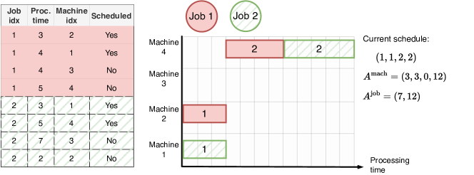
Figure 4: Example of a problem instance with $J=2$ and $M=4$. The operations’ processing times and machines are shown in the table on the left. The first two operations have already been scheduled with the partial schedule $(1,1,2,2)$. The corresponding Gantt chart and availability times are shown on the right.

This property motivates how our model is set up: For the routing problems, we have a heavy decoder that only cares about unvisited nodes and no longer about how it visited previous nodes. Similarly, for the JSSP, we are only interested in the unscheduled operations and the availability times at any time. We feed this information to a network described below.

D.5 Policy network

A suitable architecture for the JSSP should account for the fact that the problem is invariant to the job and the machine indexing (for the latter, it is only important if two operations must run on the same machine, but not which one). Our proposed architecture processes the $J\cdot M$ operations with multiple transformer layers, and we use masking to account for the indexing invariance. We make this precise as follows:

Let $A^{\text{mach}},A^{\text{job}}$ be the availability times at any constructive step. Let $i$ be the index of an unfinished job, and $m_{i}$ be the index of the machine on which the next unscheduled operation of job $i$ must run. Define $r_{i}:=\max\{A^{\text{job}}_{i},A^{\text{mach}}_{m_{i}}\}$ as the time at which this operation would start if it were scheduled next. We represent the state of the instance by $\bm{A}\in\mathbb{R}^{J\times M\times 2}$, where for $i\in\{1,\dots,J\}$ and $l\in\{1,\dots,M\}$ we set

$$\bm{A}_{i,l}=\left(\frac{p_{i,l}}{100},\frac{r_{i}-\min_{i^{\prime}\in\{1,\dots,J\}}r_{i^{\prime}}}{100}\right).$$ (33)

I.e., we repeat the start time across all operations for a job, shift the time back to 0, and scale the processing times into $[0,1]$. We affinely embed $\bm{A}$ into a latent space $\mathbb{R}^{d}$ to obtain $\hat{\bm{A}}\in\mathbb{R}^{J\times M\times d}$. We compute a sinusoidal positional encoding $\bm{P}\in\mathbb{R}^{M\times d}$ (Vaswani et al., 2017) which we add to each job $i$ via $\hat{\bm{A}}_{i}+\bm{P}$. We send the resulting sequence of operations through a stack of pairs of transformer layers, wherein each pair:

1. We use ReZero normalization (Bachlechner et al., 2021) as in the architecture for the routing problems.

2. In the first transformer layer, referred to as the ’job-wise layer’:

   • Only operations within the same job attend to each other. In practice, this can be efficiently achieved by folding the job dimension into the batch dimension, i.e., reshaping the sequence from $\mathbb{R}^{B\times J\times M\times d}$ to $\mathbb{R}^{B\cdot J\times M\times d}$.

   • We mask all operations that have already been scheduled.

   • We add ALiBi (Press et al., 2022) positional information to query-key attention scores as an attention bias in each head of a job-wise layer. Precisely, let $h$ be the number of heads, then the ALiBi-specific slope for the $k$-th head is given by the $2^{-\frac{8k}{h}}$. Then, we set the additive bias for a querying operation with index $l_{1}\in\{1,\dots,M\}$ and a key operation with index $l_{2}$ to $2^{-\frac{8k}{h}}\cdot(l_{2}-l_{1})$ for the $k$-th head. While not strictly necessary for good performance, we found that ALiBi slightly improves the results by carrying the positional information of the operations through all job-wise layers.

3. In the second transformer layer, referred to as the ’machine-wise layer’:

   • We let two operations attend to each other only if they need to run on the same machine.

   • We also mask all operations that have already been scheduled but do not employ ALiBi attention bias.

The operations transform according to different roles by repeatedly switching between job- and machine-wise layers. Note that this strategy is invariant to the job and machine indexing. In principle, it is possible to achieve a similar effect by only considering the entire sequence in $\mathbb{R}^{B\times J\cdot M\times d}$ for all transformer layers and using different masks within individual heads to account for job-wise and machine-wise attention. We settled for the switching strategy, as folding the jobs into the batch dimension practically saves computation time.

After the transformer layers, we gather the output $\bm{O}\in\mathbb{R}^{J\times d}$ corresponding to the next unscheduled operation of each job (in case the job is already finished, we take the last operation ). We apply a final transformer block on the sequence $\bm{O}$, masking already finished jobs. Afterward, we project the output to logits with a linear layer $\mathbb{R}^{d}\to\mathbb{R}$, again masking finished jobs.

Figure 5 gives an overview of the network.

Figure 5: Overview of the network architecture, using the two jobs with four operations from Figure 4. Boxes represent operations, and the numbers in the boxes indicate the machine on which it has to run. Here, we assume that the first two operations of Job 1 and the first operation of Job 2 are already scheduled. In the job-wise transformer layer, only operations within the same job attend to each other. We mask scheduled operations. We accommodate masking and ALiBi positional information in the additive attention bias (shown before scaling with slope). In the machine-wise layer, only operations running on the same machine may attend to each other, also masking scheduled operations (pink square: mask, green square: do not mask). The next possible operation is gathered for each job and used to predict the policy.

Size

We use a latent dimension of $d=64$ with three pairs of transformer layers, where each layer has eight heads and a feedforward dimension of 256. With the final transformer layer, this amounts to a total of 7 layers.

D.5.1 Gumbeldore training

We train the model with GD for 100 epochs. In each epoch, we randomly pick a $J\times M$ size in $\{10\times 15,15\times 15,15\times 20\}$. We generate 512 random instances of the chosen size for which we sample 128 solutions with GD using a beam width of $k=32$ in $n=4$ rounds. We use a fixed advantage step size of $\sigma=0.05$. We start with $p_{\text{min}}=1$ and set $p_{\text{min}}=0.95$ after 50 epochs. During supervised training on the generated solutions, given a full trajectory $(j_{1},\dots,j_{J\cdot M})$, we uniformly sample $q\in\{1,\dots,J\cdot M-1\}$ and compute $A^{\text{mach}}$ and $A^{\text{job}}$ according to the subschedule $(j_{1},\dots,j_{q-1})$. The training target is then to predict $j_{q}$. No further augmentation is performed.

As for the routing problems, we use an initial learning rate of 2e-4 and clip gradients to unit norm.

Appendix E Comparison to concurrent work

Independently of our work, Corsini et al. (2024) develop a similar learning strategy for the JSSP. They also turn away from RL and sample 256 solutions in each epoch for randomly generated instances using the current model. Then, they supervisedly train a GNN + Pointer Network on the generated solutions. They call this strategy ’self-labeling’. While our Algorithm 1 is slightly different from theirs (maintaining a best greedy policy and expanding the dataset in case of no improvement), their work and ours match in the spirit of applying behavior cloning to sampled solutions. However, Corsini et al. (2024) focus on the JSSP and their proposed GNN architecture using the disjunctive graph representation of the JSSP. Most importantly, while they discuss different sampling schemes, they settled on sampling with replacement (Monte Carlo i.i.d. sampling) from the sequence model, which they found sufficient for their approach. Our main contribution revolves around a principled way to get the most out of a few samples, applied to various neural CO problems, and we show in Section 5.3 that our method can significantly improve the sampling performance. Furthermore, we compare our method on the JSSP with their approach in Table 2. Our work is also motivated by bridging the problem that large network architectures that generalize strongly can be computationally challenging to train with policy gradient methods. However, we emphasize that we believe the work of Corsini et al. (2024) and ours are mutually reinforcing, as both conclude that a more ’straightforward’ training strategy than self-critical policy gradient methods can lead to a strong performance in neural CO.

References

- Ahn et al. (2020) Sungsoo Ahn, Younggyo Seo, and Jinwoo Shin. Learning what to defer for maximum independent sets. In International conference on machine learning, pp. 134–144. PMLR, 2020.
- Applegate et al. (2006) D.L. Applegate, R.E. Bixby, V. Chvatal, and W.J. Cook. The traveling salesman problem: a computational study. Princeton University Press, 2006.
- Bachlechner et al. (2021) Thomas Bachlechner, Bodhisattwa Prasad Majumder, Henry Mao, Gary Cottrell, and Julian McAuley. Rezero is all you need: Fast convergence at large depth. In Uncertainty in Artificial Intelligence, pp. 1352–1361. PMLR, 2021.
- Bello et al. (2016) Irwan Bello, Hieu Pham, Quoc V Le, Mohammad Norouzi, and Samy Bengio. Neural combinatorial optimization with reinforcement learning. arXiv preprint arXiv:1611.09940, 2016.
- Bengio et al. (2021) Yoshua Bengio, Andrea Lodi, and Antoine Prouvost. Machine learning for combinatorial optimization: a methodological tour d’horizon. European Journal of Operational Research, 290(2):405–421, 2021.
- Bogyrbayeva et al. (2022) Aigerim Bogyrbayeva, Meraryslan Meraliyev, Taukekhan Mustakhov, and Bissenbay Dauletbayev. Learning to solve vehicle routing problems: A survey. arXiv preprint arXiv:2205.02453, 2022.
- Chalumeau et al. (2024) Felix Chalumeau, Shikha Surana, Clément Bonnet, Nathan Grinsztajn, Arnu Pretorius, Alexandre Laterre, and Tom Barrett. Combinatorial optimization with policy adaptation using latent space search. Advances in Neural Information Processing Systems, 36, 2024.
- Chen & Tian (2019) Xinyun Chen and Yuandong Tian. Learning to perform local rewriting for combinatorial optimization. Advances in neural information processing systems, 32, 2019.
- Choo et al. (2022) Jinho Choo, Yeong-Dae Kwon, Jihoon Kim, Jeongwoo Jae, André Hottung, Kevin Tierney, and Youngjune Gwon. Simulation-guided beam search for neural combinatorial optimization. Advances in Neural Information Processing Systems, 35:8760–8772, 2022.
- Corsini et al. (2024) Andrea Corsini, Angelo Porrello, Simone Calderara, and Mauro Dell’Amico. Self-labeling the job shop scheduling problem. arXiv preprint arXiv:2401.11849, 2024.
- d O Costa et al. (2020) Paulo R d O Costa, Jason Rhuggenaath, Yingqian Zhang, and Alp Akcay. Learning 2-opt heuristics for the traveling salesman problem via deep reinforcement learning. In Asian conference on machine learning, pp. 465–480. PMLR, 2020.
- Danihelka et al. (2022) Ivo Danihelka, Arthur Guez, Julian Schrittwieser, and David Silver. Policy improvement by planning with gumbel. In International Conference on Learning Representations, 2022. URL https://openreview.net/forum?id=bERaNdoegnO.
- De Boer et al. (2005) Pieter-Tjerk De Boer, Dirk P Kroese, Shie Mannor, and Reuven Y Rubinstein. A tutorial on the cross-entropy method. Annals of operations research, 134:19–67, 2005.
- Deudon et al. (2018) Michel Deudon, Pierre Cournut, Alexandre Lacoste, Yossiri Adulyasak, and Louis-Martin Rousseau. Learning heuristics for the tsp by policy gradient. In Integration of Constraint Programming, Artificial Intelligence, and Operations Research: 15th International Conference, CPAIOR 2018, Delft, The Netherlands, June 26–29, 2018, Proceedings 15, pp. 170–181. Springer, 2018.
- Drakulic et al. (2023) Darko Drakulic, Sofia Michel, Florian Mai, Arnaud Sors, and Jean-Marc Andreoli. Bq-nco: Bisimulation quotienting for efficient neural combinatorial optimization. In Thirty-seventh Conference on Neural Information Processing Systems, 2023.
- Fu et al. (2021) Zhang-Hua Fu, Kai-Bin Qiu, and Hongyuan Zha. Generalize a small pre-trained model to arbitrarily large tsp instances. In Proceedings of the AAAI conference on artificial intelligence, volume 35, pp. 7474–7482, 2021.
- Grinsztajn et al. (2024) Nathan Grinsztajn, Daniel Furelos-Blanco, Shikha Surana, Clément Bonnet, and Tom Barrett. Winner takes it all: Training performant rl populations for combinatorial optimization. Advances in Neural Information Processing Systems, 36, 2024.
- Gumbel (1954) E.J. Gumbel. Statistical theory of extreme values and some practical applications: a series of lectures, volume 33. US Government Printing Office, 1954.
- Henderson et al. (2018) Peter Henderson, Riashat Islam, Philip Bachman, Joelle Pineau, Doina Precup, and David Meger. Deep reinforcement learning that matters. In Proceedings of the AAAI conference on artificial intelligence, volume 32, 2018.
- Holtzman et al. (2020) Ari Holtzman, Jan Buys, Li Du, Maxwell Forbes, and Yejin Choi. The curious case of neural text degeneration. In International Conference on Learning Representations, 2020. URL https://openreview.net/forum?id=rygGQyrFvH.
- Hottung & Tierney (2020) André Hottung and Kevin Tierney. Neural large neighborhood search for the capacitated vehicle routing problem. In 24th European Conference on Artificial Intelligence (ECAI 2020), 2020.
- Hottung et al. (2020) André Hottung, Bhanu Bhandari, and Kevin Tierney. Learning a latent search space for routing problems using variational autoencoders. In International Conference on Learning Representations, 2020.
- Hottung et al. (2022) André Hottung, Yeong-Dae Kwon, and Kevin Tierney. Efficient active search for combinatorial optimization problems. In International Conference on Learning Representations, 2022. URL https://openreview.net/forum?id=nO5caZwFwYu.
- Huijben et al. (2022) I.A.M. Huijben, W. Kool, M.B. Paulus, and R.J.G. van Sloun. A review of the gumbel-max trick and its extensions for discrete stochasticity in machine learning. IEEE PAMI, 45(2):1353–1371, 2022.
- Joshi et al. (2019) Chaitanya K Joshi, Thomas Laurent, and Xavier Bresson. An efficient graph convolutional network technique for the travelling salesman problem. arXiv preprint arXiv:1906.01227, 2019.
- Joshi et al. (2020) Chaitanya K Joshi, Quentin Cappart, Louis-Martin Rousseau, and Thomas Laurent. Learning the travelling salesperson problem requires rethinking generalization. arXiv preprint arXiv:2006.07054, 2020.
- Kim et al. (2021) Minsu Kim, Jinkyoo Park, et al. Learning collaborative policies to solve np-hard routing problems. Advances in Neural Information Processing Systems, 34:10418–10430, 2021.
- Kim et al. (2022) Minsu Kim, Junyoung Park, and Jinkyoo Park. Sym-NCO: Leveraging symmetricity for neural combinatorial optimization. In Alice H. Oh, Alekh Agarwal, Danielle Belgrave, and Kyunghyun Cho (eds.), Advances in Neural Information Processing Systems, 2022. URL https://openreview.net/forum?id=kHrE2vi5Rvs.
- Kingma & Ba (2014) Diederik P Kingma and Jimmy Ba. Adam: A method for stochastic optimization. arXiv preprint arXiv:1412.6980, 2014.
- Kool et al. (2019a) W. Kool, H. van Hoof, and M. Welling. Buy 4 reinforce samples, get a baseline for free! In International Conference on Learning Representations, 2019a.
- Kool et al. (2020) W. Kool, H. van Hoof, and M. Welling. Estimating gradients for discrete random variables by sampling without replacement. In International Conference on Learning Representations, 2020.
- Kool et al. (2019b) Wouter Kool, Herke van Hoof, and Max Welling. Attention, learn to solve routing problems! In International Conference on Learning Representations, 2019b. URL https://openreview.net/forum?id=ByxBFsRqYm.
- Kool et al. (2019c) Wouter Kool, Herke Van Hoof, and Max Welling. Stochastic beams and where to find them: The gumbel-top-k trick for sampling sequences without replacement. In International Conference on Machine Learning, pp. 3499–3508. PMLR, 2019c.
- Kool et al. (2022) Wouter Kool, Herke van Hoof, Joaquim Gromicho, and Max Welling. Deep policy dynamic programming for vehicle routing problems. In International conference on integration of constraint programming, artificial intelligence, and operations research, pp. 190–213. Springer, 2022.
- Kwon et al. (2020) Yeong-Dae Kwon, Jinho Choo, Byoungjip Kim, Iljoo Yoon, Youngjune Gwon, and Seungjai Min. Pomo: Policy optimization with multiple optima for reinforcement learning. Advances in Neural Information Processing Systems, 33:21188–21198, 2020.
- Li et al. (2016) J. Li, W. Monroe, and D. Jurafsky. A simple, fast diverse decoding algorithm for neural generation. arXiv preprint arXiv:1611.08562, 2016.
- Luo et al. (2023) Fu Luo, Xi Lin, Fei Liu, Qingfu Zhang, and Zhenkun Wang. Neural combinatorial optimization with heavy decoder: Toward large scale generalization. In Thirty-seventh Conference on Neural Information Processing Systems, 2023.
- Ma et al. (2021) Yining Ma, Jingwen Li, Zhiguang Cao, Wen Song, Le Zhang, Zhenghua Chen, and Jing Tang. Learning to iteratively solve routing problems with dual-aspect collaborative transformer. Advances in Neural Information Processing Systems, 34:11096–11107, 2021.
- Maddison et al. (2014) Chris J Maddison, Daniel Tarlow, and Tom Minka. A* sampling. Advances in neural information processing systems, 27, 2014.
- Nazari et al. (2018) Mohammadreza Nazari, Afshin Oroojlooy, Lawrence Snyder, and Martin Takác. Reinforcement learning for solving the vehicle routing problem. Advances in neural information processing systems, 31, 2018.
- Niu et al. (2023) Yazhe Niu, Yuan Pu, Zhenjie Yang, Xueyan Li, Tong Zhou, Jiyuan Ren, Shuai Hu, Hongsheng Li, and Yu Liu. Lightzero: A unified benchmark for monte carlo tree search in general sequential decision scenarios. In Thirty-seventh Conference on Neural Information Processing Systems Datasets and Benchmarks Track, 2023. URL https://openreview.net/forum?id=oIUXpBnyjv.
- Park et al. (2021) Junyoung Park, Jaehyeong Chun, Sang Hun Kim, Youngkook Kim, and Jinkyoo Park. Learning to schedule job-shop problems: representation and policy learning using graph neural network and reinforcement learning. International Journal of Production Research, 59(11):3360–3377, 2021.
- Park et al. (2022) Junyoung Park, Sanzhar Bakhtiyarov, and Jinkyoo Park. Schedulenet: Learn to solve multi-agent scheduling problems with reinforcement learning, 2022. URL https://openreview.net/forum?id=nWlk4jwupZ.
- Paszke et al. (2019) Adam Paszke, Sam Gross, Francisco Massa, Adam Lerer, James Bradbury, Gregory Chanan, Trevor Killeen, Zeming Lin, Natalia Gimelshein, Luca Antiga, et al. Pytorch: An imperative style, high-performance deep learning library. Advances in neural information processing systems, 32, 2019.
- Pirnay et al. (2023) Jonathan Pirnay, Quirin Göttl, Jakob Burger, and Dominik Gerhard Grimm. Policy-based self-competition for planning problems. In The Eleventh International Conference on Learning Representations, 2023. URL https://openreview.net/forum?id=SmufNDN90G.
- Press et al. (2022) Ofir Press, Noah Smith, and Mike Lewis. Train short, test long: Attention with linear biases enables input length extrapolation. In International Conference on Learning Representations, 2022. URL https://openreview.net/forum?id=R8sQPpGCv0.
- Rennie et al. (2017) S.J. Rennie, E. Marcheret, Y. Mroueh, J. Ross, and V. Goel. Self-critical sequence training for image captioning. IEEE CVPR, 2017.
- Rubinstein (1999) Reuven Rubinstein. The cross-entropy method for combinatorial and continuous optimization. Methodology and computing in applied probability, 1:127–190, 1999.
- Schulman et al. (2017) John Schulman, Filip Wolski, Prafulla Dhariwal, Alec Radford, and Oleg Klimov. Proximal policy optimization algorithms. arXiv preprint arXiv:1707.06347, 2017.
- Shi et al. (2020) Kensen Shi, David Bieber, and Charles Sutton. Incremental sampling without replacement for sequence models. In International Conference on Machine Learning, pp. 8785–8795. PMLR, 2020.
- Taillard (1993) E. Taillard. Benchmarks for basic scheduling problems. European Journal of Operational Research, 64:278–285, 1993.
- Vaswani et al. (2017) Ashish Vaswani, Noam Shazeer, Niki Parmar, Jakob Uszkoreit, Llion Jones, Aidan N Gomez, Łukasz Kaiser, and Illia Polosukhin. Attention is all you need. Advances in neural information processing systems, 30, 2017.
- Vidal (2022) Thibaut Vidal. Hybrid genetic search for the cvrp: Open-source implementation and swap* neighborhood. Computers & Operations Research, 140:105643, 2022.
- Vieira (2014) T. Vieira. Gumbel-max trick and weighted reservoir sampling. http://timvieira.github.io/blog/post/2014/08/01/gumbel-max-trick-and-weighted-reservoir-sampling/, 2014.
- Vijayakumar et al. (2018) A. Vijayakumar, M. Cogswell, R. Selvaraju, Q. Sun, S. Lee, D. Crandall, and D. Batra. Diverse beam search for improved description of complex scenes. AAAI, 2018.
- Vinyals et al. (2015) Oriol Vinyals, Meire Fortunato, and Navdeep Jaitly. Pointer networks. Advances in neural information processing systems, 28, 2015.
- Williams (1992) R.J. Williams. Simple statistical gradient-following algorithms for connectionist reinforcement learning. Machine learning, 8:229–256, 1992.
- Wu et al. (2021) Yaoxin Wu, Wen Song, Zhiguang Cao, Jie Zhang, and Andrew Lim. Learning improvement heuristics for solving routing problems. IEEE transactions on neural networks and learning systems, 33(9):5057–5069, 2021.
- Xin et al. (2021) Liang Xin, Wen Song, Zhiguang Cao, and Jie Zhang. Multi-decoder attention model with embedding glimpse for solving vehicle routing problems. In Proceedings of the AAAI Conference on Artificial Intelligence, volume 35, pp. 12042–12049, 2021.
- Yellott Jr. (1977) J.I. Yellott Jr. The relationship between luce’s choice axiom, thurstone’s theory of comparative judgment, and the double exponential distribution. Journal of Mathematical Psychology, 15(2):109–144, 1977.
- Zhang et al. (2020) Cong Zhang, Wen Song, Zhiguang Cao, Jie Zhang, Puay Siew Tan, and Xu Chi. Learning to dispatch for job shop scheduling via deep reinforcement learning. Advances in Neural Information Processing Systems, 33:1621–1632, 2020.
- Zhang et al. (2024) Cong Zhang, Zhiguang Cao, Wen Song, Yaoxin Wu, and Jie Zhang. Deep reinforcement learning guided improvement heuristic for job shop scheduling. In The Twelfth International Conference on Learning Representations, 2024. URL https://openreview.net/forum?id=jsWCmrsHHs.
- Zhao et al. (2022) Linlin Zhao, Weiming Shen, Chunjiang Zhang, and Kunkun Peng. An end-to-end deep reinforcement learning approach for job shop scheduling. In 2022 IEEE 25th International Conference on Computer Supported Cooperative Work in Design (CSCWD), pp. 841–846, 2022. doi: 10.1109/CSCWD54268.2022.9776116.