Double Cross-fit Doubly Robust Estimators:
Beyond Series Regression

Abstract

Doubly robust estimators with cross-fitting have gained popularity in causal inference due to their favorable structure-agnostic error guarantees. However, when additional structure, such as Hölder smoothness, is available then more accurate “double cross-fit doubly robust” (DCDR) estimators can be constructed by splitting the training data and undersmoothing nuisance function estimators on independent samples. We study a DCDR estimator of the Expected Conditional Covariance, a functional of interest in causal inference and conditional independence testing, and derive a series of increasingly powerful results with progressively stronger assumptions. We first provide a structure-agnostic error analysis for the DCDR estimator with no assumptions on the nuisance functions or their estimators. Then, assuming the nuisance functions are Hölder smooth, but without assuming knowledge of the true smoothness level or the covariate density, we establish that DCDR estimators with several linear smoothers are semiparametric efficient under minimal conditions and achieve fast convergence rates in the non-$\sqrt{n}$ regime. When the covariate density and smoothnesses are known, we propose a minimax rate-optimal DCDR estimator based on undersmoothed kernel regression. Moreover, we show an undersmoothed DCDR estimator satisfies a slower-than-$\sqrt{n}$ central limit theorem, and that inference is possible even in the non-$\sqrt{n}$ regime. Finally, we support our theoretical results with simulations, providing intuition for double cross-fitting and undersmoothing, demonstrating where our estimator achieves semiparametric efficiency while the usual “single cross-fit” estimator fails, and illustrating asymptotic normality for the undersmoothed DCDR estimator.

1 Introduction

In causal inference, the researcher’s objective is often to estimate a lower-dimensional functional of the data generating distribution (e.g., the Average Treatment Effect, the Local Average Treatment Effect, the Average Treatment Effect on the Treated, etc.). Depending on the functional, estimators can be constructed as summary statistics of combinations of nuisance function estimates (e.g., the propensity score and outcome regression function). For this purpose, doubly robust estimators based on influence functions and semiparametric efficiency theory have become increasingly popular due to their favorable error guarantees (van der Laan and Robins, 2003; Tsiatis, 2006; Kennedy, 2022). Doubly robust estimators can be combined with cross-fitting, where the nuisance function estimators are trained on a separate, independent sample, to avoid imposing Donsker or other complexity conditions (Chernozhukov et al., 2018; Zheng and van der Laan, 2010; Robins et al., 2008). This approach, which we refer to as the “single cross-fit” doubly robust (SCDR) estimator, is well-known and extensively studied. By employing sample splitting and cross-fitting, flexible machine learning estimators can be used to estimate nuisance functions while still guaranteeing semiparametric efficiency and asymptotic normality for the functional estimator, under $n^{-1/4}$-type rate conditions on the nuisance estimators. In fact, Balakrishnan et al. (2023) showed this estimator is minimax optimal in a particular structure-agnostic model.

However, despite its favorable structure-agnostic properties, the SCDR estimator may be sub-optimal when additional structure, such as Hölder smoothness, is present. For instance, when estimating a mixed bias functional and assuming Hölder$(s)$ smooth nuisance functions, the SCDR estimator is semiparametric efficient when $s>d/2$, where $d$ is the dimension of the covariates (Rotnitzky et al., 2021). Notably, this condition is stronger than the minimax lower bound that $s>d/4$ (Robins et al., 2009). In the non-$\sqrt{n}$ regime, when $s<d/4$, the SCDR estimator also fails to attain the lower bound on the minimax rate.

Robins et al. (2008) introduced higher-order estimators as an alternative to the SCDR estimator, using the higher-order influence function of the target functional to further debias the doubly robust (or, “first-order”) estimator. These higher-order estimators can be minimax rate-optimal and semiparametric efficient under minimal conditions in smoothness models. However, the practical construction of higher-order estimators remains challenging despite recent advances (Robins et al., 2017; van der Vaart, 2014; Liu et al., 2021; Liu and Li, 2023; Liu et al., 2020).

Another option, first proposed by Newey and Robins (2018), is the double cross-fit doubly robust (DCDR) estimator, which combines the doubly robust estimator with undersmoothed nuisance function estimators trained on separate, independent samples. Combining undersmoothing with cross-fitting and / or sample splitting for optimal estimation has been demonstrated in a variety of contexts (Giné and Nickl, 2008a; Paninski and Yajima, 2008; Newey et al., 1998; van der Laan et al., 2022). Newey and Robins (2018) proposed the DCDR estimator with regression spline nuisance function estimators and showed this estimator can be semiparametric efficient under minimal conditions in a Hölder smoothness model. Fisher and Fisher (2023) and Kennedy (2023) extended this approach to estimate heterogeneous effects, while McGrath and Mukherjee (2022) developed minimax rate-optimal plug-in and DCDR estimators, employing series estimators with wavelets to estimate the nuisance functions.

In this paper, we use a DCDR estimator to estimate the Expected Conditional Covariance (ECC), incorporating progressively stronger assumptions to yield increasingly powerful results. We begin with a structure-agnostic analysis, presenting a novel asymptotically linear expansion of the DCDR estimator and providing a detailed analysis of the remainder term. Assuming Hölder smoothness of the nuisance functions, we then establish semparametric efficiency under minimal conditions and rates of convergence in the non-$\sqrt{n}$ regime. Importantly, we consider nearest neighbors and local polynomial regression estimators for the nuisance functions, which have not been studied in this context. Furthermore, when both the smoothness levels of the nuisance functions and the covariate density are known, we show that minimax optimal estimation and slower-than-$\sqrt{n}$ inference are feasible.

1.1 Structure of the paper and our contributions

In Section 1.2 we define relevant notation. In Section 2, we describe the ECC, review known lower bounds for estimating the ECC over Hölder smoothness classes, revisit the existing literature of plug-in, doubly robust and higher-order estimators for the ECC, and discuss the motivation for double cross-fitting in more detail.

In Section 3, we provide a new structure-agnostic convergence result for generic DCDR estimators and analyze its implications, noting that undersmoothing leads to the fastest convergence rate when the nuisance functions satisfy a covariance condition — specifically, when the covariance over the training data of an estimator’s predictions at two independent test points scales inversely with sample size.

In Section 4, we assume the nuisance functions are Hölder smooth, but do not assume the smoothness or the covariate density are known, and analyze the DCDR estimator. We show that the DCDR estimator combined with undersmoothed local polynomial regression is semiparametric efficient under minimal conditions, and achieves a convergence rate in the non-$\sqrt{n}$ regime faster than that of the usual SCDR estimator. This faster convergence rate has been conjectured to be the minimax rate with non-smooth covariate density (Robins et al., 2008). We also highlight that the DCDR estimator with k-Nearest Neighbors can be semiparametric efficient when the nuisance functions are Hölder smooth of order at most one but are sufficiently smooth compared to the dimension of the covariates (e.g., if the nuisance functions are Lipschitz and the dimension of the covariates is less than four). However, none of the estimators in Section 4 achieve the minimax rate for smooth or known covariate density because the relevant tuning parameters can only scale at a certain rate to guarantee the inverse Gram matrix exists.

Therefore, in Section 5 we assume the covariate density is known, and use it to allow the tuning parameters to scale at more extreme rates and the nuisance function estimators to be further undersmoothed. We demonstrate minimax optimality of the DCDR estimator when combined with appropriately undersmoothed covariate-density-adapted kernel regression, which uses the known covariate density. Furthermore, we show asymptotic normality in the non-$\sqrt{n}$ regime by undersmoothing the DCDR estimator so its variance dominates its squared bias, but it converges to a normal limiting distribution around the ECC at a slower-than-$\sqrt{n}$ rate.

In Section 6, we illustrate our results via simulation. We provide intuition for double cross-fitting and undersmoothing, demonstrate when our estimator achieves semiparametric efficiency while the usual “single cross-fit” estimator fails, and illustrate asymptotic normality for the undersmoothed DCDR estimator in the non-$\sqrt{n}$ regime. Finally, in Section 7, we conclude and discuss future work.

This paper provides several contributions to the literature. Lemma 1 and Proposition 1 in Section 3 present a new structure-agnostic analysis of the DCDR estimator for the ECC, which holds for generic nuisance function estimators. These results can be useful for generic data generating processes and generic nuisance function estimators. Theorems 1 and 2 in Sections 4 and 5, respectively, establish semiparametric efficiency under minimal conditions and minimax rate-optimal convergence for the DCDR estimator depending on the smoothness of the nuisance functions, knowledge of the covariate density, and the nuisance function estimators. While Newey and Robins (2018) and McGrath and Mukherjee (2022) presented results for series and spline methods, our results extend these analyses to local averaging estimators such as local polynomial regression and k-Nearest Neighbors. Moreover, Theorem 3 shows asymptotic normality, allowing for inference when both the covariate density and smoothness of the nuisance functions are known. While Robins et al. (2016) established asymptotic normality of a higher-order estimator of the ECC in the non-$\sqrt{n}$-regime, our result is, to the best of our knowledge, the first limiting distribution result for a cross-fit doubly robust estimator in the non-$\sqrt{n}$ regime. Lastly, our simulation results illustrate efficiency and inference with Hölder smooth nuisance functions. Our code is available at https://github.com/alecmcclean/DCDR.

1.2 Notation

We use $\mathbb{E}$ for expectation, $\mathbb{V}$ for variance,  cov  for covariance, and $\mathbb{P}_{n}(f)=\mathbb{P}_{n}\{f(Z)\}=\frac{1}{n}\sum_{i=1}^{n}f(Z_{i})$ for sample averages. When $x\in\mathbb{R}^{d}$ we let $\lVert x\rVert^{2}=\sum_{j=1}^{d}x_{j}^{2}$ denote the squared Euclidean norm, while for generic possibly random functions $f$ we let $\lVert f\rVert_{\mathbb{P}}^{2}=\int_{\mathcal{Z}}f(z)^{2}d\mathbb{P}(z)$ denote the squared $L_{2}(\mathbb{P})$ norm and $\lVert f\rVert_{\infty}=\sup_{z\in\mathcal{Z}}|f(z)|$ denote the supremum of $f$. If $\widehat{f}$ is an estimated function, then $\mathbb{E}\lVert\widehat{f}\rVert_{\mathbb{P}}^{2}$ is the expectation of $\lVert\widehat{f}\rVert_{\mathbb{P}}^{2}$ over the training data used to construct $\widehat{f}$. Finally, if $A$ is a square matrix, then $\lambda_{i}(A)$ refers to the $i^{th}$ eigenvalue of $A$ and $\rho(A)=\max_{i}\left\{|\lambda_{i}(A)|\right\}$ is the maximum absolute eigenvalue of $A$, or spectral radius of $A$.

We use the notation $a\lesssim b$ to mean $a\leq Cb$ for some constant $C$, and $a\asymp b$ to mean $cb\leq a\leq Cb$ for some constants $c$ and $C$, so that $a\lesssim b$ and $b\lesssim a$. We use $\rightsquigarrow$ to denote convergence in distribution, $\stackrel{{\scriptstyle p}}{{\rightarrow}}$ for convergence in probability, and $\stackrel{{\scriptstyle a.s.}}{{\longrightarrow}}$ for convergence almost surely. We use the notation $a\wedge b$ and $a\vee b$ to denote the minimum and maximum, respectively, of $a$ and $b$. We use $o_{\mathbb{P}}(\cdot)$ and $O_{\mathbb{P}}(\cdot)$ to mean usual convergence in probability and stochastic boundedness, i.e., if $X_{n}$ is a sequence of random variables then $X_{n}=o_{\mathbb{P}}(r_{n})$ implies $\left|\frac{X_{n}}{r_{n}}\right|\stackrel{{\scriptstyle p}}{{\rightarrow}}0$ and $X_{n}=O_{\mathbb{P}}(r_{n})$ implies there exists $C<\infty$ such that $\mathbb{P}\left(\left|\frac{X_{n}}{r_{n}}\right|\geq C\right)\to 0$ as $n\to\infty$, and use $o(1)$ and $O(1)$ to denote usual deterministic convergence, i.e., if $x_{n}$ is a sequence then $x_{n}=o(1)$ implies $x_{n}\to 0$ as $n\to\infty$ and $x_{n}=O(1)$ implies there exists $C<\infty$ such that $x_{n}\leq C$ as $n\to\infty$.

When referring to the class of Hölder$(s)$ smooth functions, we mean the class of functions $f:\mathbb{R}^{d}\to\mathbb{R}$ that are $\lfloor s\rfloor$-times continuously differentiable with partial derivatives bounded (where $\lfloor s\rfloor$ is the largest integer strictly smaller than $s$), and for which

$$|D^{m}f(x)-D^{m}f(x^{\prime})|\lesssim\lVert x-x^{\prime}\rVert^{s-\lfloor s\rfloor}$$

for all $x,x^{\prime}$ and $m=(m_{1},\ldots,m_{d})$ such that $\sum_{j=1}^{d}m_{j}=\lfloor s\rfloor$, where $D^{m}=\frac{\partial^{\lfloor s\rfloor}}{\partial_{x_{1}}^{m_{1}}\ldots\partial_{x_{d}}^{m_{d}}}$ is the multivariate partial derivative operator.

In certain places, we denote generic nuisance functions by $\eta$. When relevant, we denote datasets of $n$ observations by $D$ with an appropriate subscript to indicate which dataset. For example, we will refer to the training data for estimating nuisance function $\eta$ by $D_{\eta}$. Further, we denote the covariates of $n$ observations by $X^{n}$, and use subscripts in the same way. So, $X^{n}_{\eta}$ denotes the covariate data in $D_{\eta}$.

2 Setup and background

In this section, we describe the data generating process and the ECC, review known lower bounds for estimating the ECC over Hölder smoothness classes, revisit the existing literature on plug-in, doubly robust, and higher-order estimators, and discuss the motivation for double cross-fitting.

We assume we observe a dataset comprising $3n$ independent and identically distributed data points $\{Z_{i}\}_{i=1}^{3n}$ drawn from a distribution $\mathcal{P}$. Here, $Z_{i}$ is a tuple $\{X_{i},A_{i},Y_{i}\}$ where $X\in\mathbb{R}^{d}$ are covariates and $A\in\mathbb{R}$ and $Y\in\mathbb{R}$. We denote $\pi(X)=\mathbb{E}(A\mid X)$ and $\mu(X)=\mathbb{E}(Y\mid X)$ and collectively refer to them as nuisance functions. In causal inference, often $A$ denotes binary treatment status, while $Y$ is the outcome of interest. In that case, $\pi$ is referred to as the propensity score and $\mu$ as the outcome regression function.

In this paper, we focus on estimating the ECC, denoted by $\psi_{ecc}$, which is defined as:

$$\psi_{ecc}=\mathbb{E}\{\hskip 0.50003pt\text{cov}\hskip 0.50003pt(A,Y\mid X)\}=\mathbb{E}(AY)-\mathbb{E}\{\pi(X)\mu(X)\}.$$

The ECC appears in the causal inference literature in the numerator of the variance weighted average treatment effect (Li et al., 2011), as a measure of causal influence (Díaz, 2023), and in derivative effects under stochastic interventions (McClean et al., 2022; Zhou and Opacic, 2022). Additionally, the ECC has appeared in the conditional independence testing literature (Shah and Peters, 2020). Prior work on semiparametric efficient and minimax optimal DCDR estimators has also focused on the ECC (McGrath and Mukherjee, 2022; Newey and Robins, 2018; Fisher and Fisher, 2023).

Remark 1.

We assume we observe $3n$ observations in total so we have $n$ observations for each independent fold. When estimating the ECC with the DCDR estimator, we split the data into three folds: two for training and one for estimation. Since our focus is on asymptotic rates, we ignore the constant factor lost from splitting the data. But, with iid data, one can cycle the folds, repeat the estimation, and take the average to retain full sample efficiency.

2.1 Assumptions and lower bounds on estimation rates

In this section, we impose two standard conditions on the data generating process. Then, we review the known lower bounds for estimating the ECC under Hölder smoothness assumptions, although we do not invoke these smoothness assumptions until Sections 4 and 5. We start with the two assumptions we impose throughout.

Assumption 1.

(Bounded first and second moments for $A$ and $Y$) The regression functions $\mu(X)$ and $\pi(X)$ satisfy $|\mu(X)|<\infty,|\pi(X)|<\infty$, and the conditional second moments of $A$ and $Y$ are bounded above and below; i.e, $0<\mathbb{V}(A\mid X=x),\mathbb{V}(Y\mid X=x)<\infty$ for all $x\in\mathcal{X}$.

We also assume the covariate density $f(X)$ is upper and lower bounded and has bounded support $\mathcal{X}$.

Assumption 2.

(Bounded covariate density) The covariates $X$ have support $\mathcal{X}$, a compact subset of $\mathbb{R}^{d}$, and the covariate density $f(x)$ satisfies $c\leq f(x)\leq C$ for all $x\in\mathcal{X}$ and $0<c\leq C<\infty$.

We require no further assumptions until Section 4. In Sections 4 and 5, we analyze the DCDR estimator when the data generating process satisfies $\pi\in\text{H\"{o}lder}(\alpha)$ and $\mu\in\text{H\"{o}lder}(\beta)$. In this regime, and when the covariate density is sufficiently smooth, Robins et al. (2008) and Robins et al. (2009) proved that the minimax rate satisfies

$$\inf_{\widehat{\psi}}\sup_{\mathcal{P}_{\alpha,\beta}}\mathbb{E}|\widehat{\psi}-\psi_{ecc}|\gtrsim\begin{cases}n^{-1/2}&\text{ if }\frac{\alpha+\beta}{2}>d/4,\\ n^{-\frac{2\alpha+2\beta}{2\alpha+2\beta+d}}&\text{otherwise.}\end{cases}$$ (1)

The minimax rate exhibits an “elbow” phenomenon, where semiparametric efficiency and $\sqrt{n}$-convergence are possible when the average smoothness of the nuisance functions is larger than $d/4$. Outside that regime, the lower bound on the minimax rate is slower than $\sqrt{n}$ and depends on the average smoothness of the nuisance functions and the dimension of the covariates. Importantly, these rates depend on the covariate density being smooth enough that it does not affect the estimation rate; when the covariate density is non-smooth, minimax rates for the ECC are not yet known.

2.2 Plug-in, doubly robust, and higher-order estimators

In this section, we describe plug-in, doubly robust, and higher-order estimators. Ultimately, we will focus on doubly robust estimators due to their simplicity and popularity.

A plug-in estimator for the ECC can be constructed based on the representation

$$\mathbb{E}\{\hskip 0.50003pt\text{cov}\hskip 0.50003pt(A,Y\mid X)\}=\mathbb{E}(AY)-\mathbb{E}\{\pi(X)\mu(X)\}$$

or

$$\mathbb{E}\{\hskip 0.50003pt\text{cov}\hskip 0.50003pt(A,Y\mid X)\}=\mathbb{E}\big{[}A\{Y-\mu(X)\}\big{]}.$$

In either case, an estimator can be constructed according to the “plugin principle”, by plugging in estimates for the relevant nuisance functions and taking the empirical average. These estimators are often intuitive and easy to construct, but they can inherit biases from their nuisance function estimators. This has inspired an extensive literature on doubly robust estimators, which are also referred to as “first-order”, “double machine learning”, or “one-step” estimators.

Doubly robust estimators are based on semiparametric efficiency theory and the efficient influence function (EIF), which acts like a functional derivative in the first-order von Mises expansion of the functional (van der Vaart and Wellner, 1996; Tsiatis, 2006). For the ECC, the un-centered EIF is

$$\varphi(Z)=\{A-\pi(X)\}\{Y-\mu(X)\}.$$ (2)

The doubly robust estimator is constructed by estimating the nuisance functions, plugging their values into the formula for the un-centered EIF, and taking the empirical average:

$$\widehat{\psi}_{dr}=\mathbb{P}_{n}\left[\{A-\widehat{\pi}(X)\}\{Y-\widehat{\mu}(X)\}\right].$$

Other doubly robust estimators such as the targeted maximum likelihood estimator are also common in the literature (van der Laan and Rose, 2011). They provide similar asymptotic guarantees as the doubly robust estimator, and are often referred to as “doubly robust” when their bias can be bounded by the product of the root mean squared errors of the nuisance function estimators. They can achieve $\sqrt{n}$-convergence even when their nuisance function estimators are estimated nonparametrically at slower rates. Furthermore, Balakrishnan et al. (2023) recently showed that the doubly robust estimator is minimax optimal in a particular structure-agnostic model. However, if extra structure is available, such as Hölder smoothness, then standard doubly robust estimators may not be minimax optimal. This has inspired a growing literature on higher-order estimators.

Higher-order estimators are based on a higher-order von Mises expansion of the functional of interest (Robins et al., 2008; Li et al., 2011). Just as doubly robust estimators correct the bias of plug-in estimators, higher-order estimators correct the bias of doubly robust estimators. For the ECC, the second-order estimator is

$$\widehat{\psi}_{hoif}=\widehat{\psi}_{dr}-\frac{1}{n(n-1)}\sum_{i\neq j}\left\{A_{i}-\widehat{\pi}(X_{i})\right\}b(X_{i})^{T}\widehat{\Sigma}^{-1}b(X_{j})\left\{Y_{j}-\widehat{\mu}(X_{j})\right\}$$

where $b(X)$ is a basis with dimension growing with sample size and $\widehat{\Sigma}=\mathbb{P}_{n}\{b(X)b(X)^{T}\}$ is the Gram matrix. Higher-order estimators capitalize on the additional structure available when the nuisance functions are smooth, enabling them to achieve the minimax rate in some settings (Robins et al., 2008, 2009). Recent research has developed adaptive and more numerically stable extensions of higher-order estimators (Liu et al., 2021; Liu and Li, 2023).

2.3 Doubly robust estimation and cross-fitting

In this section, we briefly review doubly robust estimation and cross-fitting and discuss the motivation behind double cross-fitting. For a more comprehensive discussion, see Newey and Robins (2018).

Single cross-fit doubly robust (SCDR) estimators, which train the nuisance function estimators on a separate sample from which the functional is estimated, are now relatively well-known in the literature (Chernozhukov et al., 2018; Zheng and van der Laan, 2010; Robins et al., 2008). When estimating the ECC, $\widehat{\psi}_{scdr}=\mathbb{P}_{n}\big{[}\left\{A-\widehat{\pi}(X)\right\}\left\{Y-\widehat{\mu}(X)\right\}\big{]}$, with $\widehat{\pi}$ and $\widehat{\mu}$ trained on an independent dataset from that used to calculate the sample average. Standard analysis of the SCDR estimator shows that its bias scales with the product of root mean squared errors (RMSE) of the nuisance function estimators; i.e., $\left|\mathbb{E}(\widehat{\psi}_{scdr}-\psi_{ecc})\right|\leq\lVert\widehat{\mu}-\mu\rVert_{\mathbb{P}}\lVert\widehat{\pi}-\pi\rVert_{\mathbb{P}}$. This upper bound on the bias is minimized if both nuisance functions are estimated optimally in terms of RMSE. However, if the nuisance functions are Hölder smooth, the SCDR estimator which minimizes RMSE of its nuisance function estimators may not achieve the minimax rate.

The motivation for double cross-fitting arises from a key insight into the sub-optimality of the SCDR estimator. As discussed in Newey and Robins (2018), training the nuisance functions on the same dataset introduces a dependence between the estimators, and so the bound on the bias of the SCDR estimator is minimized only when both nuisance function estimators are estimated optimally in terms of RMSE. This intuition motivates double cross-fitting, where the training data is split and the nuisance function estimators are trained on two independent folds. Then, the nuisance function estimators are independent, and the bias of the DCDR estimator only depends on the biases of the nuisance function estimators, rather than their RMSEs. And, since the variance of the DCDR estimator will be diminished via averaging in the estimation fold, it is reasonable to expect that the nuisance function estimators can be undersmoothed for faster bias convergence rates without paying a price for the excess variance. We illustrate this phenomenon in subsequent sections when we study the DCDR estimator with undersmoothed linear smoothers.

In the next section, we formally outline the DCDR estimator and derive a structure-agnostic linear expansion for its error. In Sections 4 and 5, we incorporate progressively stronger assumptions to prove increasingly powerful results, including semiparametric efficiency under minimal conditions, minimax optimality, and asymptotic normality in the non-$\sqrt{n}$ regime.

3 The DCDR estimator and a structure-agnostic linear expansion

In this section, we derive a structure-agnostic asymptotically linear expansion for the DCDR estimator which holds with generic nuisance functions and estimators. To the best of our knowledge, this is the first such structure-agnostic analysis that can allow for improved rates with undersmoothing. Then, we provide a nuisance-function-agnostic decomposition of the remainder term from the asymptotically linear expansion. Finally, we discuss, informally, how these results reveal that undersmoothing the nuisance function estimators can lead to faster convergence rates for the DCDR estimator. First, we formally outline the DCDR estimator.

Algorithm 1.

(DCDR Estimator for the ECC) Let $(D_{\mu},D_{\pi},D_{\varphi})$ denote three independent samples of $n$ observations of $Z_{i}=(X_{i},A_{i},Y_{i})$. Then:

1. Train an estimator $\widehat{\mu}$ for $\mu$ on $D_{\mu}$ and train an estimator $\widehat{\pi}$ for $\pi$ on $D_{\pi}$.

2. On $D_{\varphi}$, estimate the un-centered efficient influence function values $\widehat{\varphi}(Z)=\{A-\widehat{\pi}(X)\}\{Y-\widehat{\mu}(X)\}$ using the estimators from step 1, and construct the DCDR estimator $\widehat{\psi}_{n}$ as the empirical average of $\widehat{\varphi}(Z)$ over the estimation data $D_{\varphi}$:

   $$\widehat{\psi}_{n}=\mathbb{P}_{n}\{\widehat{\varphi}(Z)\}\equiv\frac{1}{n}\sum_{Z_{i}\in D_{\varphi}}\widehat{\varphi}(Z_{i}).$$

Our first result is a structure-agnostic asymptotically linear expansion of the DCDR estimator. It does not require any assumptions about the nuisance functions or their estimators beyond Assumptions 1 and 2.

Lemma 1.

(Structure-agnostic linear expansion) Under Assumptions 1 and 2, if $\psi_{ecc}$ is estimated with the DCDR estimator $\widehat{\psi}_{n}$ from Algorithm 1, then

$$\widehat{\psi}_{n}-\psi_{ecc} =(\mathbb{P}_{n}-\mathbb{P})\{\varphi(Z)\}+R_{1,n}+R_{2,n}$$

$$\text{ where }R_{1,n} \leq\lVert b_{\pi}\rVert_{\mathbb{P}}\lVert b_{\mu}\rVert_{\mathbb{P}}\text{ and }R_{2,n}=O_{\mathbb{P}}\left(\sqrt{\frac{\mathbb{E}\lVert\widehat{\varphi}-\varphi\rVert_{\mathbb{P}}^{2}+\rho(\Sigma_{n})}{n}}\right),$$

$b_{\eta}\equiv b_{\eta}(X)=\mathbb{E}\{\widehat{\eta}(X)-\eta(X)\mid X\}$ is the pointwise bias of the estimator $\widehat{\eta}$, $\rho(\Sigma_{n})$ denotes the spectral radius of $\Sigma_{n}$, and

$$\Sigma_{n}=\mathbb{E}\left(\hskip 0.50003pt\text{cov}\hskip 0.50003pt\left[\Big{\{}\widehat{b}_{\varphi}(X_{1}),...,\widehat{b}_{\varphi}(X_{n})\Big{\}}^{T}\mid X_{\varphi}^{n}\right]\right)$$

where $\widehat{b}_{\varphi}(X_{i})=\mathbb{E}\{\widehat{\varphi}(Z_{i})-\varphi(Z_{i})\mid X_{i},D_{\pi},D_{\mu}\}$ is the conditional bias of $\widehat{\varphi}$ and $X_{\varphi}^{n}$ denotes the covariates in the estimation sample.

All proofs are delayed to the appendix. Here, we provide some intuition for the result. Crucially, the proof of Lemma 1 analyzes the randomness of the DCDR estimator over both the estimation and training data. By contrast, the analysis of the SCDR estimator is usually conducted conditionally on the training data. The unconditional analysis of the DCDR estimator allows us to leverage the independence of the training samples, thereby bounding the bias of the DCDR estimator by the product of integrated biases of the nuisance function estimators. However, the unconditional analysis also requires accounting for the covariance over the training data between summands of the DCDR estimator because, without conditioning on the training data, the nuisance function estimators are random, and $\widehat{\varphi}(Z_{i})\cancel{\mathchoice{\mathrel{\hbox to0.0pt{$\displaystyle\perp$\hss}\mkern 4.0mu{\displaystyle\perp}}}{\mathrel{\hbox to0.0pt{$\textstyle\perp$\hss}\mkern 4.0mu{\textstyle\perp}}}{\mathrel{\hbox to0.0pt{$\scriptstyle\perp$\hss}\mkern 4.0mu{\scriptstyle\perp}}}{\mathrel{\hbox to0.0pt{$\scriptscriptstyle\perp$\hss}\mkern 4.0mu{\scriptscriptstyle\perp}}}}\widehat{\varphi}(Z_{j})$ and $\hskip 0.50003pt\text{cov}\hskip 0.50003pt_{i\neq j}\{\widehat{\varphi}(Z_{i}),\widehat{\varphi}(Z_{j})\}\neq 0$. These non-zero covariances are accounted for by the new spectral radius term in the second remainder term, $\rho(\Sigma_{n})$, which we analyze in further detail in Proposition 1.

Lemma 1 is useful because of its generality, and we use it throughout the rest of the paper. Beyond Assumptions 1 and 2, Lemma 1 requires no assumptions for the nuisance functions or their estimators. This is in contrast to previous results, which focus on specific linear smoothers for the nuisance function estimators (Newey and Robins, 2018; McGrath and Mukherjee, 2022; Kennedy, 2023; Fisher and Fisher, 2023). In Section 4, we use Lemma 1 to analyze the DCDR estimator with linear smoothers. Before that, we analyze the spectral radius term in Lemma 1 without assuming any structure on the nuisance functions or their estimators, but leveraging the specific structure of the ECC.

Remark 2.

McGrath and Mukherjee (2022) improved upon the bias term in Lemma 1 using special properties of wavelet estimators, and the bias of their estimator scales like the minimum of two bias products. We demonstrate that a similar phenomenon occurs for local polynomial regression in Section 5.

Proposition 1.

(Spectral radius bound) Under Assumptions 1 and 2, if $\psi_{ecc}$ is estimated with the DCDR estimator $\widehat{\psi}_{n}$ from Algorithm 1, then

$$\frac{\rho(\Sigma_{n})}{n}\leq\frac{\mathbb{E}\lVert\widehat{\varphi}-\varphi\rVert_{\mathbb{P}}^{2}}{n} +\left(\lVert b_{\pi}^{2}\rVert_{\infty}+\lVert s_{\pi}^{2}\rVert_{\infty}\right)\mathbb{E}\Big{[}\big{|}\hskip 0.50003pt\text{cov}\hskip 0.50003pt\{\widehat{\mu}(X_{i}),\widehat{\mu}(X_{j})\mid X_{i},X_{j}\}\big{|}\Big{]}$$

$$+\left(\lVert b_{\mu}^{2}\rVert_{\infty}+\lVert s_{\mu}^{2}\rVert_{\infty}\right)\mathbb{E}\Big{[}\big{|}\hskip 0.50003pt\text{cov}\hskip 0.50003pt\{\widehat{\pi}(X_{i}),\widehat{\pi}(X_{j})\mid X_{i},X_{j}\}\big{|}\Big{]}$$

where $\lVert b_{\eta}^{2}\lVert_{\infty}=\sup_{x\in\mathcal{X}}\mathbb{E}\{\widehat{\eta}(X)-\eta(X)\mid X=x\}^{2}$ and $\lVert s_{\eta}^{2}\rVert_{\infty}=\sup_{x\in\mathcal{X}}\mathbb{V}\{\widehat{\eta}(X)\mid X=x\}$ are uniform squared bias and variance bounds.

Here, we describe Proposition 1 in further detail. The first term on the right hand side comes from the diagonal of $\Sigma_{n}$, and is equal to the variance terms already observed in Lemma 1. The second and third terms come from the off-diagonal terms in $\Sigma_{n}$. The expected absolute covariance, $\mathbb{E}\Big{[}\big{|}\hskip 0.50003pt\text{cov}\hskip 0.50003pt\{\widehat{\eta}(X_{i}),\widehat{\eta}(X_{j})\mid X_{i},X_{j}\}\big{|}\Big{]}$, measures the covariance over the training data of an estimator’s predictions at two independent test points. For many estimators, we anticipate that $\mathbb{E}\Big{[}\big{|}\hskip 0.50003pt\text{cov}\hskip 0.50003pt\{\widehat{\eta}(X_{i}),\widehat{\eta}(X_{j})\mid X_{i},X_{j}\}\big{|}\Big{]}\lesssim n^{-1}$, and we demonstrate this to be the case for several linear smoothers subsequently.

Like Lemma 1, Proposition 1 is useful because of its generality: it applies to any nuisance functions and nuisance function estimators. Although Proposition 1 relies specifically on the functional being the ECC, we anticipate that similar results apply for other functionals.

Further investigation of Proposition 1 reveals when undersmoothing the nuisance function estimators will lead to the fastest convergence rate. The EIF of the ECC, like many functionals, is Lipschitz in terms of its nuisance functions, so $\widehat{\varphi}-\varphi\lesssim|\widehat{\pi}-\pi|+|\widehat{\mu}-\mu|$ and $\lVert\widehat{\varphi}-\varphi\rVert_{\mathbb{P}}\lesssim\lVert\widehat{\pi}-\pi\rVert_{\mathbb{P}}+\lVert\widehat{\mu}-\mu\rVert_{\mathbb{P}}$. Moreover, the compactness of the support of $X$ in Assumption 2 implies that the supremum mean squared errors of the nuisance function estimators scale at the typical pointwise rate. Therefore, if the expected covariance term scales inversely with sample size such that $\mathbb{E}\Big{[}\big{|}\hskip 0.50003pt\text{cov}\hskip 0.50003pt\{\widehat{\eta}(X_{i}),\widehat{\eta}(X_{j})\mid X_{i},X_{j}\}\big{|}\Big{]}=O_{\mathbb{P}}(n^{-1})$, then $\frac{\rho(\Sigma_{n})}{n}=O_{\mathbb{P}}\left(\frac{\mathbb{E}\lVert\widehat{\varphi}-\varphi\rVert_{\mathbb{P}}^{2}}{n}\right)=O_{\mathbb{P}}\left(\frac{\lVert b_{\pi}^{2}\rVert_{\infty}+\lVert s_{\pi}^{2}\rVert_{\infty}+\lVert b_{\mu}^{2}\rVert_{\infty}+\lVert s_{\mu}^{2}\rVert_{\infty}}{n}\right)$, and so

$$R_{2,n}=O_{\mathbb{P}}\left(\sqrt{\frac{\lVert b_{\pi}^{2}\rVert_{\infty}+\lVert s_{\pi}^{2}\rVert_{\infty}+\lVert b_{\mu}^{2}\rVert_{\infty}+\lVert s_{\mu}^{2}\rVert_{\infty}}{n}}\right).$$ (3)

Balancing $R_{2,n}$ in (3) with the bias $R_{1,n}$ in Lemma 1 requires constructing nuisance function estimators such that $\lVert b_{\pi}\rVert_{\mathbb{P}}^{2}\lVert b_{\mu}\rVert_{\mathbb{P}}^{2}\asymp\frac{\lVert s_{\pi}^{2}\rVert_{\infty}+\lVert s_{\mu}^{2}\rVert_{\infty}}{n}$. A natural way to achieve such a balance is by undersmoothing both $\widehat{\pi}$ and $\widehat{\mu}$ so their squared bias is smaller than their variance.

In this section, we have demonstrated a structure-agnostic linear expansion for the DCDR estimator and presented a nuisance-function-agnostic decomposition of its remainder term. Furthermore, we discussed how, if the nuisance function estimators satisfy $\mathbb{E}\Big{[}\big{|}\hskip 0.50003pt\text{cov}\hskip 0.50003pt\{\widehat{\eta}(X_{i}),\widehat{\eta}(X_{j})\mid X_{i},X_{j}\}\big{|}\Big{]}=O_{\mathbb{P}}(n^{-1})$, then undersmoothing the nuisance function estimators will minimize the remainder term. This is as much as we can say without any assumptions on the nuisance functions or their estimators. In the next section, we assume the nuisance functions are Hölder smooth and construct DCDR estimators with local averaging linear smoothers, and we use Lemma 1 and Proposition 1 to demonstrate the DCDR estimator’s efficiency guarantees.

4 Semiparametric efficiency under minimal conditions and non-$\sqrt{n}$ convergence

In this section, we assume the nuisance functions are Hölder smooth and construct DCDR estimators without requiring knowledge of the smoothness or covariate density. When the nuisance functions are estimated with local polynomial regression, we show the DCDR estimator is semiparametric efficient under minimal conditions and, in the non-$\sqrt{n}$ regime, converges at the conjectured minimax rate with unknown and non-smooth covariate density (Robins et al., 2008). Additionally, when the nuisance functions are estimated with k-Nearest Neighbors, we demonstrate that the DCDR estimator is semiparametric efficient when the nuisance functions are Hölder smooth of order at most one and are sufficiently smooth compared to the dimension of the covariates. First, we formally state the Hölder smoothness assumptions for the nuisance functions.

Assumption 3.

(Hölder smooth nuisance functions) The nuisance functions $\pi$ and $\mu$ are Hölder smooth, with $\pi\in\text{H\"{o}lder}(\alpha)$ and $\mu\in\text{H\"{o}lder}(\beta)$.

We focus on local averaging estimators in this section, and next we review k-Nearest Neighbors and local polynomial regression. In Appendix H, we review series regression, and establish results like those in this section for regression splines and wavelet estimators. Those results are already known (Newey and Robins, 2018; Fisher and Fisher, 2023; McGrath and Mukherjee, 2022), but we provide them for completeness and because we use different proof techniques from those considered previously.

4.1 Nuisance function estimators

We define the estimators for $\mu$ using $D_{\mu}$. The estimators for $\pi$ follow analogously with $D_{\pi}$, replacing $Y$ by $A$.

Estimator 1.

(k-Nearest Neighbors) The k-Nearest Neighbors estimator for $\mu(X)=\mathbb{E}(Y\mid X)$ is

$$\widehat{\mu}(x)=\frac{1}{k}\sum_{Z_{i}\in D_{\mu}}\mathbbold{1}\big{(}\lVert X_{i}-x\rVert\leq\lVert X_{(k)}(x)-x\rVert\big{)}Y_{i},$$ (4)

where $X_{(k)}(x)$ is the $k^{\text{th}}$ nearest neighbor of $x$ in $X_{\mu}^{n}$.

The k-Nearest Neighbors estimator is simple. However, as we see subsequently, it is unable to adapt to higher smoothness in the nuisance functions, as in nonparametric regression (Györfi et al., 2002).

Estimator 2.

(Local polynomial regression) The local polynomial regression estimator for $\mu(X)=\mathbb{E}(Y\mid X)$ is

$$\widehat{\mu}(x)=\sum_{Z_{i}\in D_{\mu}}\left\{\frac{1}{nh^{d}}b(0)^{T}\widehat{Q}^{-1}b\left(\frac{X_{i}-x}{h}\right)K\left(\frac{X_{i}-x}{h}\right)\right\}Y_{i}$$ (5)

where

$$\widehat{Q}=\frac{1}{nh^{d}}\sum_{X_{i}\in X_{\mu}^{n}}b\left(\frac{X_{i}-x}{h}\right)K\left(\frac{X_{i}-x}{h}\right)b\left(\frac{X_{i}-x}{h}\right)^{T},$$

$b:\mathbb{R}^{d}\to\mathbb{R}^{p}$ where $p={d+\lceil d/2\rceil\choose\lceil d/2\rceil}$ is a vector of orthogonal basis functions consisting of all powers of each covariate up to order $\lceil d/2\rceil$ and all interactions up to degree $\lceil d/2\rceil$ polynomials (see, Masry (1996), Belloni et al. (2015) Section 3), $\lceil d/2\rceil$ denotes the smallest integer strictly larger than $d/2$, $K:\mathbb{R}^{d}\to\mathbb{R}$ is a bounded kernel with support on $[-1,1]^{d}$, and $h$ is a bandwidth parameter. If the matrix $\widehat{Q}$ is not invertible, $\widehat{\mu}(x)=0$.

Local polynomial regression has been extensively studied (Ruppert and Wand, 1994; Masry, 1996; Fan and Gijbels, 2018; Tsybakov, 2009). There are two notable features to this version of the estimator. First, the basis is expanded to order $\lceil d/2\rceil$, the smallest integer strictly larger than $d/2$, rather than the smoothness of the regression function. Therefore, the estimator does not require knowledge of the true smoothness, but the expansion of the basis to degree $\lceil d/2\rceil$ still ensures the bias of the DCDR estimator is $o_{\mathbb{P}}(n^{-1/2})$ in the $\sqrt{n}$-regime. Second, the estimator is explicitly defined even when the local Gram matrix, $\widehat{Q}$, is not invertible — $\widehat{\mu}(x)=0$. This ensures the bias of the estimator is bounded when $\widehat{Q}$ is not invertible.

Unlike k-Nearest Neighbors, local polynomial regression can optimally estimate functions of higher smoothness. In Appendix B, we provide bias and variance bounds for both estimators, which follow from standard results in the relevant literature (Biau and Devroye, 2015; Tsybakov, 2009; Kennedy, 2023; Györfi et al., 2002). However, two nuances arise in this analysis because the bias and variance bounds account for randomness over the training data. First, the pointwise variance, $\mathbb{V}\{\widehat{\eta}(x)\}$, scales at the typical conditional (on the training data) mean squared error rate; e.g., for local polynomial regression, $\mathbb{V}\{\widehat{\mu}(x)\}\lesssim h^{-2\beta}+\frac{1}{nh^{d}}$. It may be possible to improve this with more careful analysis, but because this will not affect the behavior of the DCDR estimator — which uses undersmoothed nuisance function estimators — we leave this to future work. Second, for local polynomial regression, the local Gram matrix $\widehat{Q}$ may not be invertible. Therefore, it is necessary to show that non-invertibility occurs with asymptotically negligible probability if the bandwidth $h$ decreases slowly enough, which is possible using a matrix Chernoff inequality (see, Tropp (2015) Section 5).

Next, we show the covariance terms from Proposition 1, $\mathbb{E}\Big{[}\big{|}\hskip 0.50003pt\text{cov}\hskip 0.50003pt\big{\{}\widehat{\eta}(X_{i}),\widehat{\eta}(X_{j})\mid X_{i},X_{j}\big{\}}\big{|}\Big{]}$, can decrease inversely with sample size for both estimators, and demonstrate the efficiency guarantees of the DCDR estimator.

4.2 Semiparametric efficiency under minimal conditions

The efficiency of the DCDR estimator depends on how quickly the expected absolute covariance $\mathbb{E}\Big{[}\big{|}\hskip 0.50003pt\text{cov}\hskip 0.50003pt\{\widehat{\eta}(X_{i}),\widehat{\eta}(X_{j})\mid X_{i},X_{j}\}\big{|}\Big{]}$ decreases. Therefore, first, we show that this term can decrease inversely with sample size for k-Nearest Neighbors and local polynomial regression.

Lemma 2.

(Covariance bound) Suppose Assumptions 1, 2, and 3 hold. Moreover, assume that each estimator balances squared bias and variance or is undersmoothed. Then, both k-Nearest Neighbors and local polynomial regression satisfy

$$\mathbb{E}\Big{[}\big{|}\hskip 0.50003pt\text{cov}\hskip 0.50003pt\{\widehat{\eta}(X_{i}),\widehat{\eta}(X_{j})\mid X_{i},X_{j}\}\big{|}\Big{]}=O_{\mathbb{P}}\left(\frac{1}{n}\right)$$ (6)

for $\eta\in\{\pi,\mu\}$.

Lemma 2 demonstrates that the expected absolute covariance can decrease inversely with sample size for both k-Nearest Neighbors and local polynomial regression. The result follows from a localization argument — if the estimation points $X_{i}$ and $X_{j}$ are well separated, then $\widehat{\eta}(X_{i})$ and $\widehat{\eta}(X_{j})$ share no training data and therefore their covariance is zero; otherwise, the covariance is upper bounded by the variance. Lemma 2 guarantees that the expected absolute covariance decreases inversely with sample size if the estimators balance squared bias and variance or are undersmoothed. It may be possible to improve this result so that it also applies to oversmoothed estimators, but because we focus only on undersmoothed nuisance function estimators subsequently, we leave that to future work.

The following result establishes that the DCDR estimator achieves semiparametric efficiency under minimal conditions and fast convergence rates in the non-$\sqrt{n}$ regime.

Theorem 1.

(Semiparametric efficiency) Suppose Assumptions 1, 2, and 3 hold, and $\psi_{ecc}$ is estimated with the DCDR estimator $\widehat{\psi}_{n}$ from Algorithm 1.

• If the nuisance functions $\widehat{\mu}$ and $\widehat{\pi}$ are estimated with local polynomial regression (Estimator 2) with bandwidths satisfying $h_{\mu},h_{\pi}\asymp\left(\frac{n}{\log n}\right)^{-1/d}$, then

  $$\begin{cases}\sqrt{\frac{n}{\mathbb{V}\{\varphi(Z)\}}}(\widehat{\psi}_{n}-\psi_{ecc})\rightsquigarrow N(0,1)&\text{ if }\frac{\alpha+\beta}{2}>d/4\text{, and}\\[10.0pt] \mathbb{E}|\widehat{\psi}_{n}-\psi_{ecc}|=O_{\mathbb{P}}\left(\frac{n}{\log n}\right)^{-\frac{\alpha+\beta}{d}}&\text{ otherwise.}\end{cases}$$ (7)

• If the nuisance functions $\widehat{\mu}$ and $\widehat{\pi}$ are estimated with k-Nearest Neighbors (Estimator 1) and $k_{\mu},k_{\pi}\asymp\log n$, then

  $$\begin{cases}\sqrt{\frac{n}{\mathbb{V}\{\varphi(Z)\}}}(\widehat{\psi}_{n}-\psi_{ecc})\rightsquigarrow N(0,1)&\text{ if }\frac{\alpha+\beta}{2}>d/4\text{ and }\alpha,\beta\leq 1\text{, and}\\[10.0pt] \mathbb{E}|\widehat{\psi}_{n}-\psi_{ecc}|\lesssim\left(\frac{n}{\log n}\right)^{-\frac{(\alpha\wedge 1)+(\beta\wedge 1)}{d}}&\text{ otherwise.}\end{cases}$$ (8)

Theorem 1 shows that the DCDR estimator with undersmoothed local polynomial regression is semiparametric efficient under minimal conditions. Further, it attains (up to a log factor) the convergence rate $n^{-\frac{\alpha+\beta}{d}}$ in probability in the non-$\sqrt{n}$ regime. This is slower than the known lower bound for estimating the ECC when the covariate density is appropriately smooth, but has been conjectured to be the minimax rate when the covariate density is non-smooth (Robins et al., 2009). A similar but weaker result holds for k-nearest Neighbors estimators, whereby the DCDR estimator achieves semiparametric efficiency when the nuisance functions are Hölder smooth of order at most one but are sufficiently smooth compared to the dimension of the covariates. A simple example is if the nuisance functions are Lipschitz (i.e., $\alpha=\beta=1$) and the dimension of the covariates is less than four ($d<4$).

The DCDR estimator based on local polynomial regression in Theorem 1 is not minimax optimal because the bandwidth is constrained so that the local Gram matrix is invertible with high probability, thereby limiting the convergence rate of the bias of the local polynomial regression estimators and, by extension, the bias of the DCDR estimator. By replacing the Gram matrix with its expectation (assuming it is known), an estimator could be undersmoothed even further for a faster bias convergence rate. In the next section we propose such an estimator — the “covariate-density-adapted” kernel regression. We illustrate that the DCDR estimator with covariate-density-adapted kernel regression can be minimax optimal. Moreover, we establish asymptotic normality in the non-$\sqrt{n}$ regime by undersmoothing the DCDR estimator so its variance dominates its squared bias, but it converges to a normal limiting distribution around the ECC at a slower-than-$\sqrt{n}$ rate.

Remark 3.

When the DCDR estimator achieves semiparametric efficiency, Slutsky’s theorem and Theorem 1 imply that inference can be conducted for the ECC with Wald-type $1-\alpha$ confidence intervals, $\widehat{\psi}_{n}\pm\Phi^{-1}(1-\alpha/2)\sqrt{\frac{\widehat{\mathbb{V}}\{\varphi(Z)\}}{n}},$ where $\widehat{\mathbb{V}}\{\varphi(Z)\}$ is any consistent estimator for $\mathbb{V}\{\varphi(Z)\}$ (e.g., the sample variance of $\widehat{\varphi}(Z)$).

Remark 4.

There are simple ad-hoc guidelines for scaling the bandwidth like $\left(\frac{n}{\log n}\right)^{-1/d}$ for local polynomial regression. For example, one could choose the smallest bandwidth for which the estimator is defined at every point in the estimation sample.

5 Minimax optimality and asymptotic normality in the non-$\sqrt{n}$ regime

In this section, we assume the covariate density is known and examine the behavior of the DCDR estimator with covariate-density-adapted kernel regression estimators for the nuisance functions. For the results in this section, we require, in addition to previous assumptions, that the covariate density is known and sufficiently smooth.

Assumption 4.

(Known, lower bounded, and smooth covariate density) The covariate density $f$ is known and $f\in\text{H\"{o}lder}(\gamma)$, where $\gamma\geq\alpha\vee\beta$.

Under Assumption 4, we demonstrate the DCDR estimator is minimax optimal. First, we define the covariate-density-adapted kernel regression estimator:

Estimator 3.

(Covariate-density-adapted kernel regression) The covariate-density-adapted kernel regression estimator for $\mu(X)=\mathbb{E}(Y\mid X)$ is

$$\widehat{\mu}(x)=\sum_{Z_{i}\in D_{\mu}}\frac{K_{\mu}\left(\frac{X_{i}-x}{h_{\mu}}\right)}{nh_{\mu}^{d}f(X_{i})}Y_{i},$$ (9)

where $h_{\mu}$ is the bandwidth and $K_{\mu}$ is a kernel (to be chosen subsequently). The estimator for $\pi(X)=\mathbb{E}(A\mid X)$ is defined analogously on $D_{\pi}$.

This estimator uses the known covariate density in the denominator of (9). As a result, no constraint on the bandwidth is required, and the estimator can be undersmoothed more than the local polynomial regression estimator in Estimator 2. McGrath and Mukherjee (2022) proposed a similar adaptation of the standard wavelet estimator. As they showed for the wavelet estimator, the known covariate density in Estimator 3 could be replaced by the estimated covariate density, and our subsequent results would follow if the covariate density were sufficiently smooth (smoother than in Assumption 4) and its estimator sufficiently accurate. Because the properties of such an estimator are not well understood when the covariate density is not sufficiently smooth, we leave this analysis to future work.

The subsequent analysis combines two versions of covariate-density-adapted kernel regression, with different kernels.

Estimator 3a.

(Higher-order covariate-density-adapted kernel regression) The higher-order covariate-density-adapted kernel regression has symmetric and bounded kernel $K$ that is of order $\lceil\alpha+\beta\rceil$ and satisfies $K(x/h)\lesssim\mathbbold{1}(\lVert x\rVert\leq h)$, $\int K(x)dx=1$, $\int K(x)^{2}dx\asymp 1$, and $\int\lVert x\rVert^{\alpha+\beta}K(x)dx\lesssim 1$ (Györfi et al., 2002; Tsybakov, 2009).

This version of the estimator uses a higher-order localized kernel, which allows it to adapt to the sum of the smoothnesses of the nuisance functions. See, e.g., Section 5.3, Györfi et al. (2002) and Section 1.2.2, Tsybakov (2009) for a review of higher-order kernels and how to construct bounded kernels of arbitrary order. To complement this estimator, we require a smooth estimator.

Estimator 3b.

(Smooth covariate-density-adapted kernel regression) The smooth covariate-density-adapted kernel regression has continuous and bounded kernel $K$ satisfying $K(x/h)\lesssim\mathbbold{1}\left(\lVert x\rVert\leq h\right),\int K(x)dx=1$, $\int K(x)^{2}dx\asymp 1$.

Because the kernel in the smooth estimator is localized and continuous, it allows the DCDR estimator to adapt to the sum of smoothnesses of the nuisance functions through the higher-order kernel estimator. For this purpose, the smooth kernel must be continuous, but need not control higher-order bias terms. Therefore, a simple kernel is adequate, such as the Epanechnikov kernel — $K(x)=\frac{3}{4}\left(1-\lVert x\rVert^{2}\right)\mathbbold{1}\left(\lVert x\rVert\leq 1\right)$.

5.1 Minimax optimality

The following result shows that the DCDR estimator using covariate-density-adapted kernel regression estimators is minimax optimal.

Theorem 2.

(Minimax optimality) Suppose Assumptions 1, 2, 3, and 4 hold. If $\psi_{ecc}$ is estimated with the DCDR estimator $\widehat{\psi}_{n}$ from Algorithm 1, one nuisance function is estimated with the smooth covariate-density-adapted kernel regression (Estimator 3b) with bandwidth decreasing at any rate such that the estimator is consistent, and the other nuisance function is estimated with the higher-order covariate-density-adapted kernel regression (Estimator 3a) with bandwidth that scales at $n^{\frac{-2}{2\alpha+2\beta+d}}$, then

$$\begin{cases}\sqrt{\frac{n}{\mathbb{V}\{\varphi(Z)\}}}(\widehat{\psi}_{n}-\psi_{ecc})\rightsquigarrow N(0,1)&\text{ if }\frac{\alpha+\beta}{2}>d/4,\\[10.0pt] \mathbb{E}|\widehat{\psi}_{n}-\psi_{ecc}|=O_{\mathbb{P}}\left(n^{-\frac{2\alpha+2\beta}{2\alpha+2\beta+d}}\right)&\text{ otherwise.}\end{cases}$$ (10)

Theorem 2 establishes that the DCDR estimator with covariate-density-adapted kernel regression estimators is semiparametric efficient under minimal conditions and minimax optimal in the non-$\sqrt{n}$ regime. The result relies on knowledge of the smoothness of the nuisance functions, as well as shrinking one of the two bandwidths faster than $n^{-1/d}$. The proof relies on the smoothing properties of convolutions and an adaptation of Theorem 1 from Giné and Nickl (2008a), as well as results from Giné and Nickl (2008b) and Chapter 4 of Giné and Nickl (2021). While Theorem 2 is the first result applied to local averaging estimators such as kernel regression, McGrath and Mukherjee (2022) proved the same result using approximate wavelet kernel projection estimators for the nuisance functions. Their result relies on the orthogonality (in expectation) of the wavelet estimator’s predictions and residuals.

Remark 5.

To guarantee asymptotic normality in the $\sqrt{n}$-regime, it is necessary that the smooth covariate-density-adapted estimator is consistent. If one were only interested in convergence rates, as in McGrath and Mukherjee (2022), one could replace the smooth estimator by any smooth estimator with bounded variance. Indeed, supposing without loss of generality that $\widehat{\mu}$ were the higher-order kernel estimator, one could set $\widehat{\pi}=0$ and use the plug-in estimator for the ECC instead of the DCDR estimator.

5.2 Slower-than-$\sqrt{n}$ CLT

In addition to minimax optimality, asymptotic normality is possible in the non-$\sqrt{n}$ regime. The DCDR estimator in Theorem 2 balances bias and variance; intuitively, if the DCDR estimator were undersmoothed one might expect it to converge to a Normal distribution centered at the ECC at a sub-optimal slower-than-$\sqrt{n}$ rate. We demonstrate this in the next result. First, we incorporate two further assumptions.

Assumption 5.

(Boundedness) There exists $M>0$ such that $|A|<M$ and $|Y|<M$.

Assumption 6.

(Continuous conditional variance) $\mathbb{V}(A\mid X=x)$ and $\mathbb{V}(Y\mid X=x)$ are continuous in $x$.

Assumption 5 asserts that $A$ and $Y$ are bounded. Assumption 6 dictates that the conditional variances of $A$ and $Y$ are continuous in $X$, which is used to show that the limit of the standardizing variance in (12) exists. It may be possible to relax these assumptions with more careful analysis. Nonetheless, with them it is possible to establish the following result.

Theorem 3.

(Slower-than-$\sqrt{n}$ CLT) Under the conditions of Theorem 2, suppose $\frac{\alpha+\beta}{2}<\frac{d}{4}$ and Assumptions 5 and 6 hold. Suppose $\widehat{\mu}$ is the undersmoothed nuisance function estimator with bandwidth $h_{\mu}$ scaling at $n^{-\frac{2+\varepsilon}{2\alpha+2\beta+d}}$ for $0<\varepsilon<\frac{4(\alpha+\beta)}{d}$ while $\widehat{\pi}$ is the smooth consistent estimator. Then,

$$\sqrt{\frac{n}{\mathbb{V}\{\widehat{\varphi}(Z)\mid D_{\pi},D_{\mu}\}}}(\widehat{\psi}_{n}-\psi_{ecc})\rightsquigarrow N(0,1).$$ (11)

Moreover,

$$nh_{\mu}^{d}\mathbb{V}\{\widehat{\varphi}(Z)\mid D_{\pi},D_{\mu}\}\stackrel{{\scriptstyle a.s.}}{{\longrightarrow}}\mathbb{E}\left\{\frac{\mathbb{V}(A\mid X)Y^{2}}{f(X)}\right\}\mathbb{E}\left\{\frac{K_{\mu}(X)^{2}}{f(X)}\right\},$$ (12)

where $K_{\mu}$ is the kernel for $\widehat{\mu}$. If the roles of $\widehat{\mu}$ and $\widehat{\pi}$ were reversed, then (11) holds and

$$nh_{\pi}^{d}\mathbb{V}\{\widehat{\varphi}(Z)\mid D_{\pi},D_{\mu}\}\stackrel{{\scriptstyle a.s.}}{{\longrightarrow}}\mathbb{E}\left\{\frac{\mathbb{V}(Y\mid X)A^{2}}{f(X)}\right\}\mathbb{E}\left\{\frac{K_{\pi}(X)^{2}}{f(X)}\right\}.$$ (13)

Theorem 3 shows that the DCDR estimator can be suitably undersmoothed in the non-$\sqrt{n}$ regime so the DCDR estimator is sub-optimal but converges to a Normal distribution around the ECC. Moreover, Theorem 3 establishes that the conditional variance by which the error is standardized converges almost surely to a constant which can be estimated from the data. Therefore, Wald-type confidence intervals for the ECC can be constructed using (11) and (12) or (13). As far as we are aware, this is the first result demonstrating slower-than-$\sqrt{n}$ inference for a cross-fit estimator of a causal functional.

Here, we give some intuition for the result, which might best be understood through its unorthodox denominator in the standardization term in (11): the conditional variance of the estimated efficient influence function. This denominator is unorthodox both because it includes an estimated efficient influence function and because it is a conditional variance. The estimated efficient influence function arises because $\widehat{\psi}_{n}$ is undersmoothed to such an extent that its scaled variance, $\mathbb{V}\left(\sqrt{n}\widehat{\psi}_{n}\right)$, is growing with sample size. Similarly, $\mathbb{V}\{\widehat{\varphi}(Z)\mid D_{\pi},D_{\mu}\}$ is also growing at the same rate with sample size, and thus standardizing by this term appropriately concentrates the variance of the standardized statistic, $\sqrt{\frac{n}{\mathbb{V}\{\widehat{\varphi}(Z)\mid D_{\pi},D_{\mu}\}}}(\widehat{\psi}_{n}-\psi_{ecc})$. Indeed, (12) demonstrates that $\mathbb{V}\{\widehat{\varphi}(Z)\mid D_{\pi},D_{\mu}\}$ is growing with sample size because $nh_{\mu}^{d}\to 0$ as $n\to\infty$ by the assumption on the bandwidth. This result relies on a bound for higher moments of a U-statistic (Proposition 2.1, Giné et al. (2000)) which guarantees control of the sum of off-diagonal terms in $\mathbb{V}\{\widehat{\varphi}(Z)\mid D_{\pi},D_{\mu}\}$.

Meanwhile, the conditional variance is required so that a normal limiting distribution can be attained. While the non-$\sqrt{n}$ regime is often characterized by non-normal limiting distributions, a normal limiting distribution can be established applying the Berry-Esseen inequality (Theorem 1.1, Bentkus and Götze (1996)) after conditioning on the training data and showing that the standardized statistic satisfies a conditional central limit theorem almost surely and, therefore, an unconditional central limit theorem.

This approach — using sample splitting to conduct inference — is an old method which has recently been examined in several contexts, including, for example, estimating U-statistics (Robins et al., 2016; Kim and Ramdas, 2024), estimating variable importance measures (Rinaldo et al., 2019), high-dimensional model selection (Wasserman and Roeder, 2009), and post-selection inference (Meinshausen and Bühlmann, 2010; Dezeure et al., 2015). Earlier references include Cox (1975), Hartigan (1969), and Moran (1973).

While this section and previous sections have established several theoretical results for the DCDR estimator, in the next section we investigate and illustrate these properties via simulation.

6 Simulations

In this section, we study the performance of double cross-fit doubly robust (DCDR) estimators compared to single cross-fit doubly robust (SCDR) estimators and the limiting distributions of both estimators. First, we provide evidence for why undersmoothing will be optimal with the double cross-fit estimator by showing that the double cross-fit estimator requires undersmoothed nuisance function estimators to achieve the lowest error. Then, we construct Hölder smooth nuisance functions and examine when the distribution of standardized SCDR and DCDR estimates converge to standard Gaussians, and the coverage and power of Wald-style confidence intervals. Our simulations demonstrate that the undersmoothed DCDR estimator, presented in Theorem 3, enables inference via a central limit theorem in the non-$\sqrt{n}$ regime. Further, the DCDR estimator utilizing local polynomial regression without knowledge of the covariate density, as described in Theorem 1, achieves semiparametric efficiency under minimal conditions. Additionally, we observe that when the nuisance functions exhibit sufficient roughness, the SCDR estimator fails to support inference, whereas the DCDR estimators continue to do so.

All code and analysis is available at https://github.com/alecmcclean/DCDR

6.1 Intuition for undersmoothing

First, we reinforce our understanding for why double cross-fitting leads to undersmoothing the nuisance function estimators. We consider the data generating process where $X$ is uniform, $A=Y$, and both nuisance functions are the Doppler function (shown in Figure 1). Because $A=Y$, the ECC is the variance of the error noise in $A$ and $Y$. Formally, the data generating process is

$$X \sim\text{Unif}(0,1),$$ (14)

$$\pi(X)=\mu(X) =\sqrt{X(1-X)}\sin\left(\frac{2.1\pi}{X+0.05}\right),$$ (15)

$$A=Y =\pi(X)+\varepsilon,\varepsilon\sim N(0,\psi_{ecc}=0.1).$$ (16)

We chose $\psi_{ecc}=0.1$ to give a strong signal to noise ratio for the estimators. The plot of $Y$ against $X$ is shown in Figure 1.

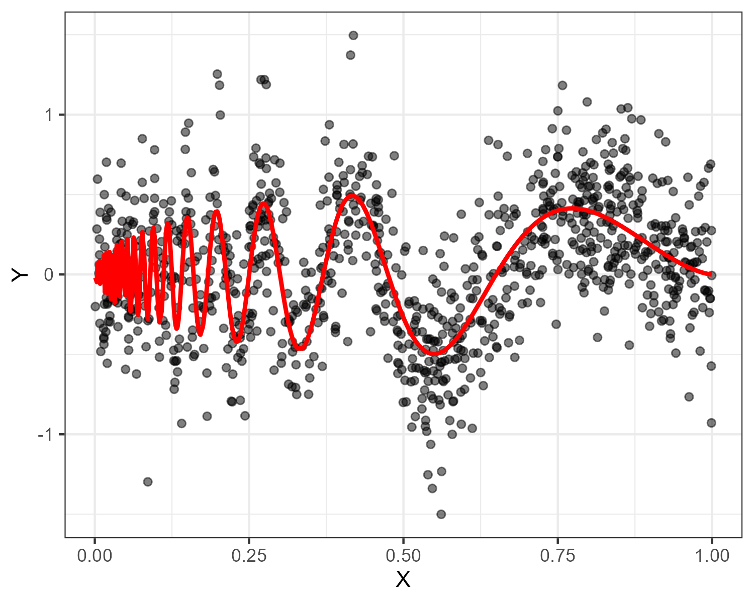
Figure 1: The Doppler function with $N(0,0.1)$ random noise as in (15); this nuisance function was used for Figure 2.

We generated $500$ datasets with three folds of sizes $\{50,100,200,500,1000,2000\}$ and estimated each nuisance function with k-Nearest Neighbors for $k$ from $1$ to $30$. We estimated the ECC with the DCDR estimator and the SCDR estimator; for the SCDR estimator we trained the nuisance functions on the same fold and discarded the unused third fold (see Remark 6). For each $k$, we computed the average mean squared error (MSE) of the nuisance function estimators and the DCDR and SCDR estimators over $500$ datasets.

To understand when undersmoothing is optimal, we calculated the optimal $k$ corresponding to the lowest average MSE over $500$ datasets for the DCDR, SCDR, and nuisance function estimators. Figure 2 displays the optimal number of neighbors (y-axis) for each fold size (x-axis), with different colors denoting estimator/estimand combinations. For instance, the green point in the bottom left corner signifies that $k=2$ gave the lowest average MSE over $500$ repetitions for the DCDR estimator estimating the ECC with datasets with folds of size $50$. The black points and line represent the optimal $k$ for $\widehat{\pi}$ estimating $\pi$, orange represent $\widehat{\mu}$ estimating $\mu$, blue represent the SCDR estimator estimating the ECC, and green represents the DCDR estimator estimating the ECC (blue, orange, and black are the same line for the most part, so the blue line completely obscures the orange and partially obscures the black). Figure 2 demonstrates the anticipated phenomenon: the optimal number of neighbors is lower for the DCDR estimator compared to the SCDR estimator and the nuisance function estimators, and it increases at a slower rate as sample size increases. Equivalently, the optimal $k$ for the DCDR estimator corresponds to undersmoothed nuisance function estimators while the optimal $k$ for the SCDR estimator corresponds to optimal nuisance function estimators.

Remark 6.

Figure 2 does not describe whether the SCDR estimator or DCDR estimator is more accurate, nor is that the goal of this analysis. Because we discarded a third of the data available to the SCDR estimator, it is not possible to compare the estimators directly. Instead, Figure 2 shows that the DCDR estimator requires undersmoothed nuisance function estimators for optimal accuracy, while the SCDR estimator requires optimal nuisance function estimators.

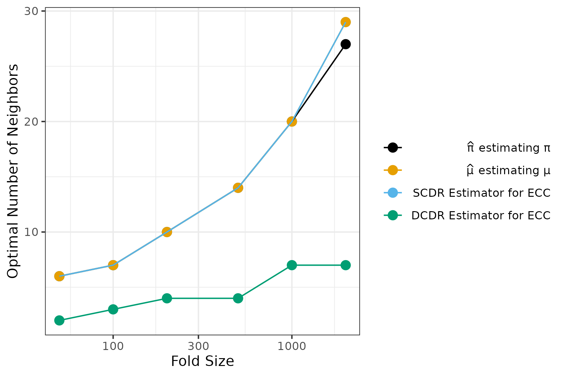
Figure 2: Fold size (x-axis) versus optimal number of neighbors (y-axis), where optimal is in terms of average MSE over 500 datasets; black and orange indicate the k-Nearest Neighbors estimators for $\pi(X)$ and $\mu(X)$, respectively, while blue indicates the SCDR estimator for the ECC and black the DCDR estimator for the ECC.

6.2 DCDR and SCDR estimators with Hölder smooth nuisance functions

In this section, we demonstrate the improved efficiency and inference possible with the DCDR estimator compared to the SCDR estimator. When the nuisance functions are Hölder smooth, the DCDR estimator with local polynomial regression can be semiparametric efficient under minimal conditions without knowledge of the covariate density or the smoothness of the nuisance functions, as in Theorem 1. Meanwhile, the SCDR estimator can only achieve semiparametric efficiency when the average smoothness is greater than half the dimension. Furthermore, we illustrate that the undersmoothed DCDR estimator can achieve inference at all non-$\sqrt{n}$ smoothness levels when the covariate density and smoothness are known, as in Theorem 3.

To facilitate our analysis, we constructed suitably smooth nuisance functions. Specifically, we consider both 1-dimensional and 4-dimensional covariates uniform on the unit cube, $\psi_{ecc}=10$, and $\pi$ and $\mu$ Hölder smooth. Throughout, we set both nuisance functions $\pi$ and $\mu$ to be of the same smoothness such that $\alpha=\beta=s$, and we control the smoothness $s$. To construct appropriately smooth functions, we employed the lower bound minimax construction for regression (see, Tsybakov (2009), pg. 92). These functions vary with sample size, and Figure 3 provides an illustration for $d=1$, with smoothness levels $s\in\{0.1,0.35,0.6\}$ and dataset sizes $N\in\{100,1000,5000\}$. To generate 4-dimensional Hölder smooth functions, we added four functions that are univariate Hölder smooth in each dimension.

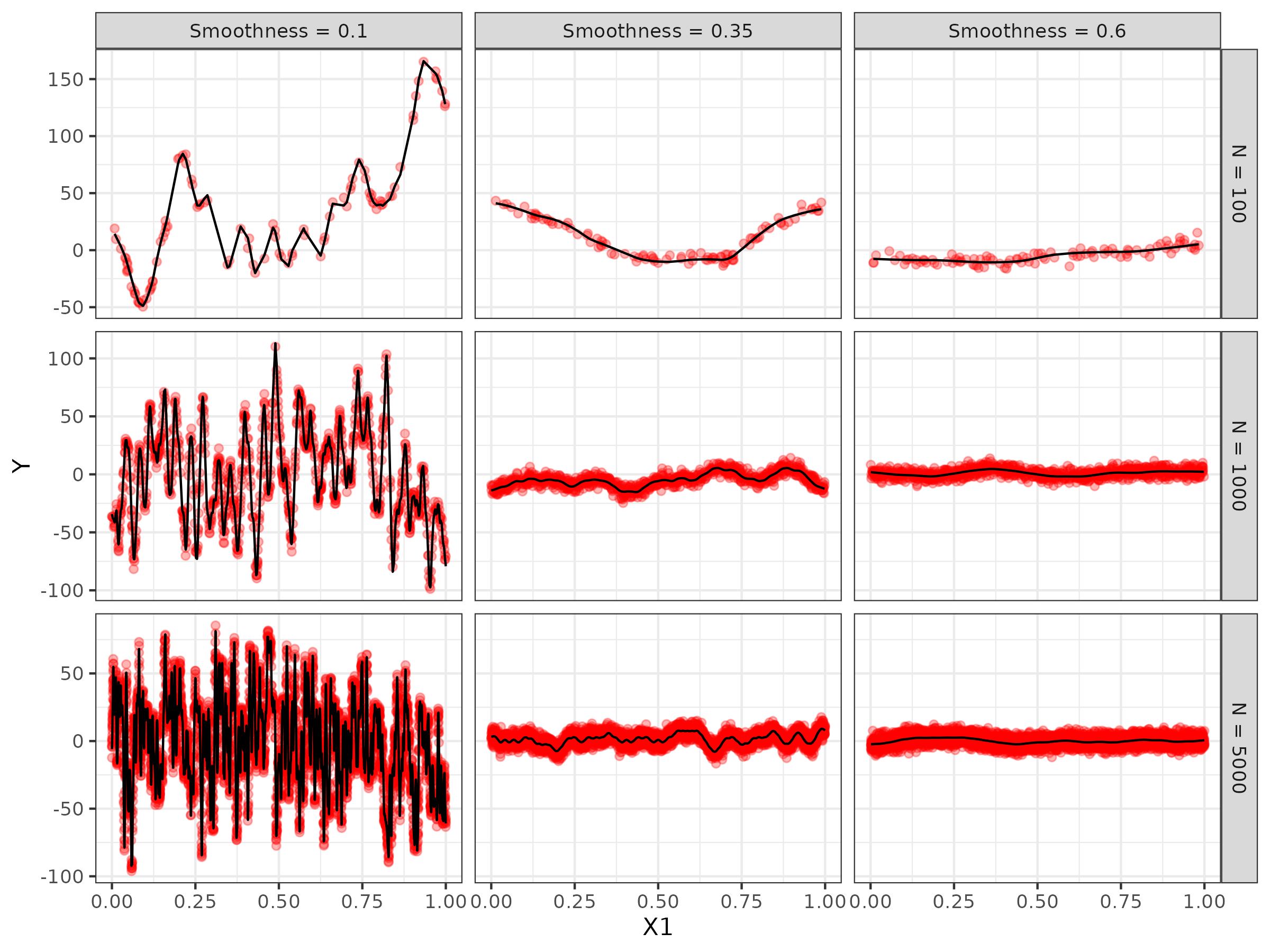
Figure 3: Example Holder smooth functions (black) of order $s\in\{0.1,0.35,0.6\}$ smoothness for $n\in\{100,1000,5000\}$ observed data points (red) with $N(0,10)$ random noise.

We generated datasets for fold sizes $\{100,200,500,1000,2000,5000\}$. When $d=1$, we constructed nuisance functions with smoothnesses $\{0.1,0.35,0.6\}$, and when $d=4$ with smoothnesses $\{0.6,1.5,2.5\}$. The first smoothness level corresponds to the non-$\sqrt{n}$ regime, the second smoothness level to the $\sqrt{n}$ regime where the SCDR estimator fails to achieve $\sqrt{n}$ efficiency, and the final level where both estimators are $\sqrt{n}$ efficient. For each fold size-dimension-smoothness combination, we generated $100$ datasets and calculated the DCDR estimator and SCDR estimator with covariate-density-adapted kernel regressions (Estimator 3). For only $d=1$, we also constructed the DCDR estimator with local polynomial regression (Estimator 2).

Figures 4 illustrates our results. Figure 4(a) shows QQ Plots for the standardized statistics for different smoothnesses (rows) and fold sizes (columns) for dimension equal to one. The black dots represent the undersmoothed DCDR estimators based on covariate-density-adapted kernel regression where the density and smoothnesses are known, while the orange dots represent the estimator based on local polynomial regression where the covariate density and smoothness are unknown. The blue dots represent the SCDR estimator based on optimal covariate-density-adapted kernel regressions that use the known covariate density and smoothnesses, which have MSE scaling at the optimal rate. The diagonal line is $y=x$. Figure 4(b) displays the coverage and power of the associated Wald-type confidence intervals, with the dimension and smoothness varying by column, and the sample size on the x-axis.

The results in Figure 4 confirm that non-$\sqrt{n}$ inference is possible, as in Theorem 3. As the sample size increases (moving across the panels in Figure 4(a)), the quantiles of the undersmoothed DCDR estimates in black converge to the quantiles of the standard normal distribution. Additionally, as sample size increases (moving across the x-axis in Figure 4(b)), the coverage of the confidence intervals approach appropriate coverage. These findings align with what was anticipated by the limiting distribution result in Theorem 3. This occurs even when $s<d/4$.

Figure 4 also confirms that the DCDR estimator facilitates inference when the SCDR estimator does not. Theorem 1 dictates that the DCDR estimator with local polynomial regression is semiparametric efficient and asymptotically normal when $d/4<s<d/2$ (the middle row). This is demonstrated in Figure 4: in Figure 4(a), when $s>d/4$, the quantiles of the unknown density DCDR estimator with local polynomial regression, as in Theorem 1, converge to the quantiles of the standard normal. However, the quantiles diverge when $s<d/4$, as shown by the orange dots in the top row. Similarly, in Figure 4(b), the confidence intervals achieve the appropriate 95% coverage when $s>d/4$, and fail otherwise. For the SCDR estimator with asymptotically optimal nuisance function estimators, Figure 4 illustrates the analogous phenomenon around the $s=d/2$ threshold. When $s>d/2$, the SCDR quantiles in the bottom row of Figure 4(a) converge closely to the normal quantiles, and do not converge otherwise. The same phenomenon occurs for the confidence intervals, which do not achieve appropriate coverage when $s<d/2$. In summary, these results support the theoretical conclusion that the DCDR estimators are semiparametric efficient and asymptotically normal in sufficiently non-smooth regimes ($d/4<s<d/2$) where the SCDR estimator is not.

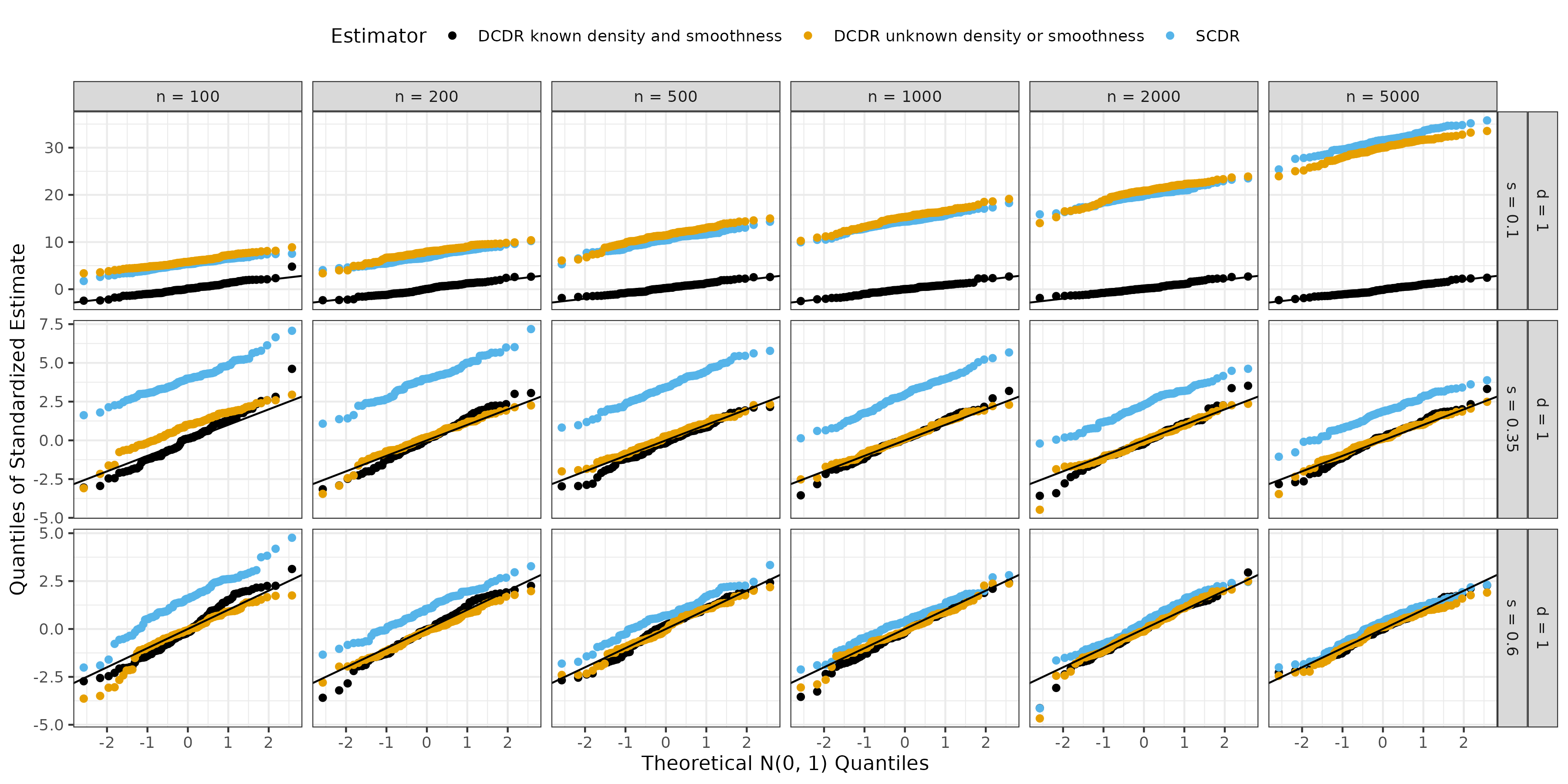
(a) QQ Plots for the standardized statistics for different dimensions and smoothnesses (columns) and fold sizes (rows). Black dots represent the undersmoothed DCDR estimator from Theorem 3 with covariate-density-adapted kernel regression (Estimator 3), orange dots represent the DCDR estimator from Theorem 1 based on local polynomial regression (Estimator 2), and blue dots represent the SCDR estimator based on covariate-density-adapted kernel regression (Estimator 3) with error scaling optimally asymptotically. The diagonal line is $y=x$.

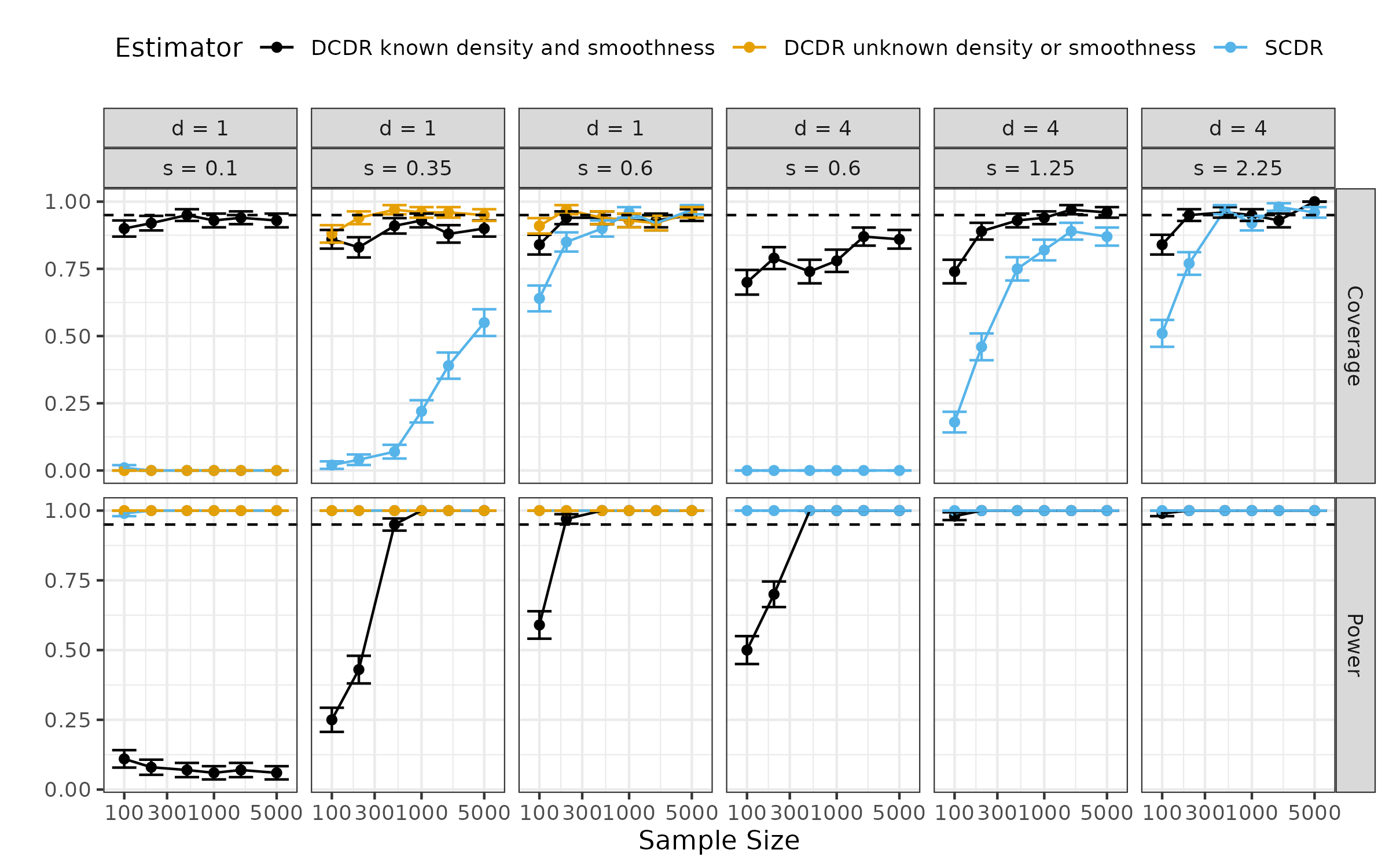
(b) Points represent the coverage (top rows) and power (bottom row) of 95% confidence intervals over $100$ datasets constructed for different dimensions and smoothnesses (columns) and fold sizes (x-axis). Error bars represent 95% confidence intervals for the coverage and power of Wald-type confidence intervals. Black represents the undersmoothed DCDR estimator from Theorem 3 with covariate-density-adapted kernel regression (Estimator 3), orange represents the DCDR estimator from Theorem 1 based on local polynomial regression (Estimator 2), and blue represents the SCDR estimator based on covariate-density-adapted kernel regression (Estimator 3) with error scaling at optimally asymptotically.

Figure 4: Illustrating the efficiency and inferential properties of double cross-fit versus single cross-fit doubly robust estimators.

7 Discussion

In this paper, we studied a double cross-fit doubly robust (DCDR) estimator for the Expected Conditional Covariance (ECC). We analyzed the estimator with progressively stronger assumptions and proved increasingly powerful results. We first derived a structure-agnostic error analysis for the DCDR estimator, which holds for generic data generating processes and nuisance function estimators. We observed that a faster convergence rate is possible by undersmoothing the nuisance function estimators, provided that these estimators satisfy a covariance condition. We established that several linear smoothers satisfy this covariance condition, and focused on the DCDR estimator with local averaging estimators for the nuisance functions, which had not been studied previously. We showed that the DCDR estimator based on undermoothed local polynomial regression is semiparametric efficient under minimal conditions without knowledge of the covariate density or the smoothness of the nuisance functions. When the covariate density is known, we demonstrated that the DCDR estimator based on undersmoothed covariate-density-adapted kernel regression is minimax optimal. Moreover, we proved an undersmoothed DCDR estimator satisfies a slower-than-$\sqrt{n}$ central limit theorem. Finally, we conducted simulations that support our findings, providing intuition for double cross-fitting and undersmoothing, demonstrating where the DCDR estimator is semiparametric efficient while the usual “single cross-fit” doubly robust estimator is not, and illustrating slower-than-root-n asymptotic normality for the undersmoothed DCDR estimator in the non-$\sqrt{n}$ regime.

There are several potential extensions of our work. While we focus on the ECC, the principles applied here generalize. Newey and Robins (2018) derived general results for the class of “average linear functionals” (Newey and Robins (2018), Section 3), and similarly general results might be possible for the larger class of “mixed bias functionals” (Rotnitzky et al., 2021). Furthermore, DCDR estimators could be used to estimate even more complex causal inference functionals, such as those based on stochastic interventions, instrumental variables, or sensitivity analyses. Achieving this would entail developing principled approaches for undersmoothing estimators of non-standard nuisance functions.

Moreover, even within the context of estimating the ECC there are still unresolved questions. When the covariate density is unknown and non-smooth, the minimax lower bound is yet unknown. Once a comprehensive understanding of the lower bound across all Hölder smoothness classes is obtained, a natural question arises regarding the feasibility of constructing adaptive and optimally efficient estimators across all smoothness classes. Finally, similar questions regarding efficiency and inference could be explored under different structural assumptions for the data generating process. For instance, one could consider nuisance functions that are sparse or have bounded variation norm and investigate the corresponding estimators.

Appendix

These supplemental materials are arranged into eight sections:

1. In Appendix A, we prove Lemma 1 and Proposition 1 from Section 3.

2. In Appendix B, we prove bias, variance, and covariance bounds for the nuisance function estimators considered in Section 4 — k-Nearest Neighbors and local polynomial regression.

3. In Appendix C, we use the results from Appendices A and B to prove Lemma 2 and Theorem 1 from Section 4.

4. In Appendix D, we prove a variety of results for covariate-density-adapted kernel regression, including conditional and unconditional variance upper and lower bounds.

5. In Appendix E, we prove Theorems 2 and 3 from Section 5, making use of the results in Appendix D.

6. In Appendix F, we prove three technical results regarding properties of the covariate density.

7. In Appendix G, we provide a simple strong law of large numbers for triangular arrays of bounded random variables.

8. Finally, in Appendix H, we review series regression nuisance function estimators, and state and prove several results based on these estimators, which are equivalent to Lemma 2 and Theorem 1 in Section 4 of the paper.

Appendix A Section 3 proofs: Lemma 1 and Proposition 1

See 1

Proof.

We first expand $\widehat{\psi}_{n}-\psi_{ecc}$ into the term in the statement of the lemma plus two remainder terms, $R_{1}$ and $R_{2}$:

$$\widehat{\psi}_{n}-\psi_{ecc} =\mathbb{P}_{n}\{\widehat{\varphi}(Z)\}-\mathbb{E}\{\varphi(Z)\}$$

$$=(\mathbb{P}_{n}-\mathbb{E})\{\varphi(Z)\}+\underbrace{\mathbb{E}\{\widehat{\varphi}(Z)-\varphi(Z)\}}_{R_{1,n}}+\underbrace{(\mathbb{P}_{n}-\mathbb{E})\{\widehat{\varphi}(Z)-\varphi(Z)\}}_{R_{2,n}}$$ (17)

where $\mathbb{E}$ refers to expectation over the estimation and training data. The first term in (17) appears in the statement of the lemma, so we manipulate it no further.

$R_{1,n}$ and bounding the bias of $\widehat{\psi}_{n}$:

The second term in (17), $R_{1,n}$, is the bias of the estimator $\widehat{\psi}_{n}$. It is not random. A simple analysis shows

$$\mathbb{E}\{\widehat{\varphi}(Z)-\varphi(Z)\} \equiv\mathbb{E}\left[\{A-\widehat{\pi}(X)\}\{Y-\widehat{\mu}(X)\}-\{A-\pi(X)\}\{Y-\mu(X)\}\right]$$

$$=\mathbb{E}\big{[}\{A-\widehat{\pi}(X)\}\{\mu(X)-\widehat{\mu}(X)\}+\{Y-\mu(X)\}\{\pi(X)-\widehat{\pi}(X)\}\big{]}$$

$$=\mathbb{E}\big{[}\{\widehat{\pi}(X)-\pi(X)\}\{\widehat{\mu}(X)-\mu(X)\}\big{]}$$

where the final line follows by iterated expectations. By the independence of the training datasets, we have

$$\mathbb{E}\big{[}\{\widehat{\pi}(X)-\pi(X)\}\{\widehat{\mu}(X)-\mu(X)\}\big{]}=\mathbb{E}\big{[}\mathbb{E}\{\widehat{\pi}(X)-\pi(X)\mid X\}\mathbb{E}\{\widehat{\mu}(X)-\mu(X)\mid X\}\big{]}\leq\lVert b_{\pi}\rVert_{\mathbb{P}}\lVert b_{\mu}\rVert_{\mathbb{P}}$$

where the inequality follows by Cauchy-Schwarz and the definition of $b_{\eta}=\mathbb{E}\{\widehat{\eta}(X)-\eta(X)\mid X\}$.

$R_{2,n}$ and bounding the variance of $\widehat{\psi}_{n}$:

The final term in (17), $R_{2,n}$, is centered and mean-zero. The statement in Lemma 1 is implied by Chebyshev’s inequality after bounding the variance of $R_{2,n}$. Thus, the rest of this proof is devoted to a bound on $\mathbb{V}(R_{2,n})$, which must account for randomness across both the estimation and training samples.

Since $\mathbb{E}\{\widehat{\varphi}(Z)-\varphi(Z)\}$ is not random, and by successive applications of the law of total variance, we have

$$\mathbb{V}\left[(\mathbb{P}_{n}-\mathbb{E})\{\widehat{\varphi}(Z)-\varphi(Z)\}\right] =\mathbb{E}\left(\mathbb{V}\Big{[}\mathbb{P}_{n}\{\widehat{\varphi}(Z)-\varphi(Z)\}\mid X^{n}_{\varphi},D_{\pi},D_{\mu}\Big{]}\right)+\mathbb{V}\left(\mathbb{E}\Big{[}\mathbb{P}_{n}\{\widehat{\varphi}(Z)-\varphi(Z)\}\mid X^{n}_{\varphi},D_{\pi},D_{\mu}\Big{]}\right)$$

$$=\mathbb{E}\left(\mathbb{V}\Big{[}\mathbb{P}_{n}\{\widehat{\varphi}(Z)-\varphi(Z)\}\mid X^{n}_{\varphi},D_{\pi},D_{\mu}\Big{]}\right)$$ (18)

$$\hskip 7.22743pt+\mathbb{E}\left\{\mathbb{V}\left(\mathbb{E}\Big{[}\mathbb{P}_{n}\{\widehat{\varphi}(Z)-\varphi(Z)\}\mid X^{n}_{\varphi},D_{\pi},D_{\mu}\Big{]}\mid X^{n}_{\varphi}\right)\right\}$$ (19)

$$\hskip 7.22743pt+\mathbb{V}\left\{\mathbb{E}\left(\mathbb{E}\Big{[}\mathbb{P}_{n}\{\widehat{\varphi}(Z)-\varphi(Z)\}\mid X^{n}_{\varphi},D_{\pi},D_{\mu}\Big{]}\mid X^{n}_{\varphi}\right)\right\}$$ (20)

where $X_{\varphi}^{n}$ are the covariates in the estimation data. Expression (18) can be upper bounded using the fact that the data are iid and $\mathbb{V}(X)\leq\mathbb{E}(X^{2})$:

$$\mathbb{E}\left(\mathbb{V}\Big{[}\mathbb{P}_{n}\{\widehat{\varphi}(Z)-\varphi(Z)\}\mid X^{n}_{\varphi},D_{\pi},D_{\mu}\Big{]}\right)=\mathbb{E}\left[\frac{1}{n}\mathbb{V}\Big{\{}\widehat{\varphi}(Z)-\varphi(Z)\mid X^{n}_{\varphi},D_{\pi},D_{\mu}\Big{\}}\right]\leq\frac{\mathbb{E}\Big{[}\{\widehat{\varphi}(Z)-\varphi(Z)\}^{2}\Big{]}}{n}.$$

Similarly expression (20) can be upper bounded using linearity of expectation, iid data, and that $\mathbb{V}(X)\leq\mathbb{E}(X^{2})$ and Jensen’s inequality:

$$\mathbb{V}\left\{\mathbb{E}\left(\mathbb{E}\Big{[}\mathbb{P}_{n}\{\widehat{\varphi}(Z)-\varphi(Z)\}\mid X^{n}_{\varphi},D_{\pi},D_{\mu}\Big{]}\mid X^{n}_{\varphi}\right)\right\} =\mathbb{V}\left(\mathbb{E}\Big{[}\mathbb{P}_{n}\{\widehat{\varphi}(Z)-\varphi(Z)\}\mid X^{n}_{\varphi}\Big{]}\right)$$

$$=\mathbb{V}\left(\mathbb{P}_{n}\Big{[}\mathbb{E}\{\widehat{\varphi}(Z)-\varphi(Z)\mid X^{n}_{\varphi}\}\Big{]}\right)$$

$$=\frac{1}{n^{2}}\sum_{i=1}^{n}\mathbb{V}\Big{[}\mathbb{E}\{\widehat{\varphi}(Z_{i})-\varphi(Z_{i})\mid X^{n}_{\varphi}\}\Big{]} \leq\frac{\mathbb{E}\Big{[}\{\widehat{\varphi}(Z)-\varphi(Z)\}^{2}\Big{]}}{n}.$$

Finally, for expression (19), by linearity of expectation, and the definition of $\widehat{b}_{\varphi}(X_{i})$ and $\Sigma_{n}$, we have

$$\mathbb{E}\left\{\mathbb{V}\left(\mathbb{E}\Big{[}\mathbb{P}_{n}\{\widehat{\varphi}(Z)-\varphi(Z)\}\mid X^{n}_{\varphi},D_{\pi},D_{\mu}\Big{]}\mid X^{n}_{\varphi}\right)\right\} =\mathbb{E}\left[\mathbb{V}\left\{\frac{1}{n}\sum_{i=1}^{n}\widehat{b}_{\varphi}(X_{i})\mid X_{\varphi}^{n}\right\}\right]$$

$$=\frac{1}{n^{2}}\sum_{i=1}^{n}\sum_{j=1}^{n}\mathbb{E}\left[\hskip 0.50003pt\text{cov}\hskip 0.50003pt\left\{\widehat{b}_{\varphi}(X_{i}),\widehat{b}_{\varphi}(X_{j})\mid X_{\varphi}^{n}\right\}\right]$$

$$=\frac{1}{n^{2}}\mathbbold{1}^{T}\Sigma_{n}\mathbbold{1}$$

where $\mathbbold{1}$ the $n$-length vector of $1$’s. Since $\Sigma_{n}$ is positive semi-definite and symmetric, $\Sigma_{n}=Q\Lambda Q^{T}$ where $Q$ is the orthonormal eigenvector matrix and $\Lambda=\text{diag}(\lambda_{1},...,\lambda_{n})$ is the diagonal eigenvalue matrix. Then,

$$\mathbbold{1}^{T}\Sigma_{n}\mathbbold{1}=\mathbbold{1}^{T}Q\Lambda Q^{T}\mathbbold{1}=\sum_{i=1}^{n}\lambda_{i}\lVert q_{i}\rVert^{2}=\sum_{i=1}^{n}\lambda_{i}\leq n\rho(\Sigma_{n})$$

where the third equality follows because the $q_{i}$ are normalized, and the inequality follows by the definition of the spectral radius. Therefore, $\frac{1}{n^{2}}\mathbbold{1}^{T}\Sigma_{n}\mathbbold{1}\leq\frac{1}{n}\rho(\Sigma_{n})$, and the result follows. ∎

See 1

Proof.

Since the spectral radius of a matrix is less than its Frobenius norm and the data are iid,

$$\frac{\rho(\Sigma_{n})}{n}\leq\frac{1}{n}\mathbb{E}\left[\mathbb{V}\left\{\widehat{b}_{\varphi}(X)\mid X_{\varphi}^{n}\right\}\right]+\frac{n-1}{n}\mathbb{E}\left[\hskip 0.50003pt\text{cov}\hskip 0.50003pt_{i\neq j}\left\{\widehat{b}_{\varphi}(X_{i}),\widehat{b}_{\varphi}(X_{j})\mid X_{\varphi}^{n}\right\}\right].$$

For the first summand, we have

$$\frac{1}{n}\mathbb{E}\left[\mathbb{V}\left\{\widehat{b}_{\varphi}(X)\mid X_{\varphi}^{n}\right\}\right]\leq\frac{\mathbb{E}\lVert\widehat{\varphi}-\varphi\rVert_{\mathbb{P}}^{2}}{n}$$

because $\mathbb{V}(X)\leq\mathbb{E}(X^{2})$. For $i\neq j$, we must analyze the covariance term in more detail. Omitting arguments (e.g., $\pi_{i}\equiv\pi(X_{i})$),

$$\mathbb{E} \left[\hskip 0.50003pt\text{cov}\hskip 0.50003pt\left\{\widehat{b}_{\varphi}(X_{i}),\widehat{b}_{\varphi}(X_{j})\mid X_{\varphi}^{n}\right\}\right]=\mathbb{E}\left\{\hskip 0.50003pt\text{cov}\hskip 0.50003pt\Big{[}\mathbb{E}\{\widehat{\varphi}(Z_{i})-\varphi(Z_{i})\mid X^{n}_{\varphi},D_{\pi},D_{\mu}\},\mathbb{E}\{\widehat{\varphi}(Z_{j})-\varphi(Z_{j})\mid X^{n}_{\varphi},D_{\pi},D_{\mu}\}\mid X^{n}_{\varphi}\Big{]}\right\}$$

$$=\mathbb{E}\left[\hskip 0.50003pt\text{cov}\hskip 0.50003pt\Big{\{}(\widehat{\pi}_{i}-\pi_{i})(\widehat{\mu}_{i}-\mu_{i}),(\widehat{\pi}_{j}-\pi_{j})(\widehat{\mu}_{j}-\mu_{j})\mid X_{i},X_{j}\Big{\}}\right]$$

$$=\mathbb{E}\left[\mathbb{E}\Big{\{}(\widehat{\pi}_{i}-\pi_{i})(\widehat{\mu}_{i}-\mu_{i})(\widehat{\pi}_{j}-\pi_{j})(\widehat{\mu}_{j}-\mu_{j})\mid X_{i},X_{j}\Big{\}}-\mathbb{E}\Big{\{}(\widehat{\pi}_{i}-\pi_{i})(\widehat{\mu}_{i}-\mu_{i})\mid X_{i},X_{j}\Big{\}}\mathbb{E}\Big{\{}(\widehat{\pi}_{j}-\pi_{j})(\widehat{\mu}_{j}-\mu_{j})\mid X_{i},X_{j}\Big{\}}\right]$$

$$=\mathbb{E}\left[\mathbb{E}\Big{\{}(\widehat{\pi}_{i}-\pi_{i})(\widehat{\pi}_{j}-\pi_{j})\mid X_{i},X_{j}\Big{\}}\mathbb{E}\Big{\{}(\widehat{\mu}_{i}-\mu_{i})(\widehat{\mu}_{j}-\mu_{j})\mid X_{i},X_{j}\Big{\}}\right]$$

$$\hskip 36.135pt-\mathbb{E}\left\{\mathbb{E}\big{(}\widehat{\pi}_{i}-\pi_{i}\mid X_{i}\big{)}\mathbb{E}\big{(}\widehat{\mu}_{i}-\mu_{i}\mid X_{i}\big{)}\mathbb{E}\big{(}\widehat{\pi}_{j}-\pi_{j}\mid X_{j}\big{)}\mathbb{E}\big{(}\widehat{\mu}_{j}-\mu_{j}\mid X_{j}\big{)}\right\}$$

$$=\mathbb{E}\left[\left\{\hskip 0.50003pt\text{cov}\hskip 0.50003pt\Big{(}\widehat{\pi}_{i},\widehat{\pi}_{j}\mid X_{i},X_{j}\Big{)}+\mathbb{E}\Big{(}\widehat{\pi}_{i}-\pi_{i}\mid X_{i}\Big{)}\mathbb{E}\Big{(}\widehat{\pi}_{j}-\pi_{j}\mid X_{j}\Big{)}\right\}\left\{\hskip 0.50003pt\text{cov}\hskip 0.50003pt\Big{(}\widehat{\mu}_{i},\widehat{\mu}_{j}\mid X_{i},X_{j}\Big{)}+\mathbb{E}\Big{(}\widehat{\mu}_{i}-\mu_{i}\mid X_{i}\Big{)}\mathbb{E}\Big{(}\widehat{\mu}_{j}-\mu_{j}\mid X_{j}\Big{)}\right\}\right]$$

$$-\mathbb{E}\left\{\mathbb{E}\big{(}\widehat{\pi}_{i}-\pi_{i}\mid X_{i}\big{)}\mathbb{E}\big{(}\widehat{\mu}_{i}-\mu_{i}\mid X_{i}\big{)}\mathbb{E}\big{(}\widehat{\pi}_{j}-\pi_{j}\mid X_{j}\big{)}\mathbb{E}\big{(}\widehat{\mu}_{j}-\mu_{j}\mid X_{j}\big{)}\right\}$$

$$=\mathbb{E}\left\{\hskip 0.50003pt\text{cov}\hskip 0.50003pt\Big{(}\widehat{\pi}_{i},\widehat{\pi}_{j}\mid X_{i},X_{j}\Big{)}\mathbb{E}(\widehat{\mu}_{i}-\mu_{i}\mid X_{i})\mathbb{E}(\widehat{\mu}_{j}-\mu_{j}\mid X_{j})\right\}+$$ (21)

$$+\mathbb{E}\left\{\hskip 0.50003pt\text{cov}\hskip 0.50003pt\Big{(}\widehat{\mu}_{i},\widehat{\mu}_{j}\mid X_{i},X_{j}\Big{)}\mathbb{E}(\widehat{\pi}_{i}-\pi_{i}\mid X_{i})\mathbb{E}(\widehat{\pi}_{j}-\pi_{j}\mid X_{j})\right\}$$ (22)

$$+\mathbb{E}\left\{\hskip 0.50003pt\text{cov}\hskip 0.50003pt\Big{(}\widehat{\pi}_{i},\widehat{\pi}_{j}\mid X_{i},X_{j}\Big{)}\hskip 0.50003pt\text{cov}\hskip 0.50003pt\Big{(}\widehat{\mu}_{i},\widehat{\mu}_{j}\mid X_{i},X_{j}\Big{)}\right\}$$ (23)

where the first equality follows by definition, the second and third by the definition of $\widehat{\varphi},\varphi$, and covariance, the fourth by the independence of the training datasets, the fifth again by the definition of covariance and because $\pi_{i},\pi_{j},\mu_{i},\mu_{j}$ are not random conditional on $X_{i},X_{j}$, and the final line by canceling terms.

For (21),

$$\mathbb{E}\left\{\hskip 0.50003pt\text{cov}\hskip 0.50003pt\Big{(}\widehat{\pi}_{i},\widehat{\pi}_{j}\mid X_{i},X_{j}\Big{)}\mathbb{E}(\widehat{\mu}_{i}-\mu_{i}\mid X_{i})\mathbb{E}(\widehat{\mu}_{j}-\mu_{j}\mid X_{j})\right\}\leq$$

$$\hskip 108.405pt\mathbb{E}\left[\left|\hskip 0.50003pt\text{cov}\hskip 0.50003pt\Big{\{}\widehat{\pi}(X_{i}),\widehat{\pi}(X_{j})\mid X_{i},X_{j}\Big{\}}\right|\right]\sup_{x_{i},x_{j}\in\mathcal{X}}\Big{|}\mathbb{E}\{\widehat{\mu}(x_{i})-\mu(x_{i})\}\mathbb{E}\{\widehat{\mu}(x_{j})-\mu(x_{j})\}\Big{|}$$

$$\hskip 108.405pt=\mathbb{E}\left[\left|\hskip 0.50003pt\text{cov}\hskip 0.50003pt\Big{\{}\widehat{\pi}(X_{i}),\widehat{\pi}(X_{j})\mid X_{i},X_{j}\Big{\}}\right|\right]\left\{\sup_{x\in\mathcal{X}}\Big{|}\mathbb{E}\{\widehat{\mu}(x)-\mu(x)\}\Big{|}\right\}^{2}$$

$$\hskip 108.405pt\leq\mathbb{E}\left[\left|\hskip 0.50003pt\text{cov}\hskip 0.50003pt\Big{\{}\widehat{\pi}(X_{i}),\widehat{\pi}(X_{j})\mid X_{i},X_{j}\Big{\}}\right|\right]\sup_{x\in\mathcal{X}}\mathbb{E}\{\widehat{\mu}(x)-\mu(x)\}^{2}$$

$$\hskip 108.405pt\equiv\mathbb{E}\left[\left|\hskip 0.50003pt\text{cov}\hskip 0.50003pt\Big{\{}\widehat{\pi}(X_{i}),\widehat{\pi}(X_{j})\mid X_{i},X_{j}\Big{\}}\right|\right]\lVert b_{\mu}^{2}\rVert_{\infty}$$

where the first inequality is Hölder’s inequality, the second because $|ab|=|a||b|$, the penultimate by Jensen’s inequality, and the final by the definition of $\lVert b_{\mu}\rVert_{\infty}$. The same result applies for (22) with $\mu$ and $\pi$ swapped. Next, notice that,

$$\hskip 0.50003pt\text{cov}\hskip 0.50003pt\Big{\{}\widehat{\pi}(X_{i}),\widehat{\pi}(X_{j})\mid X_{i},X_{j}\Big{\}} =\mathbb{E}\left(\Big{[}\widehat{\pi}(X_{i})-\mathbb{E}\{\widehat{\pi}(X_{i})\mid X_{i},X_{j}\}\Big{]}\Big{[}\widehat{\pi}(X_{j})-\mathbb{E}\{\widehat{\pi}(X_{j})\mid X_{i},X_{j}\}\Big{]}\mid X_{i},X_{j}\right)$$

$$=\mathbb{E}\left(\Big{[}\widehat{\pi}(X_{i})-\mathbb{E}\{\widehat{\pi}(X_{i})\mid X_{i}\}\Big{]}\Big{[}\widehat{\pi}(X_{j})-\mathbb{E}\{\widehat{\pi}(X_{j})\mid X_{j}\}\Big{]}\mid X_{i},X_{j}\right)$$

$$\leq\sqrt{\mathbb{E}\left(\Big{[}\widehat{\pi}(X_{i})-\mathbb{E}\{\widehat{\pi}(X_{i})\mid X_{i}\}\Big{]}^{2}\mid X_{i}\right)\mathbb{E}\left(\Big{[}\widehat{\pi}(X_{j})-\mathbb{E}\{\widehat{\pi}(X_{j})\mid X_{j}\}\Big{]}^{2}\mid X_{j}\right)}$$

$$=\sqrt{\mathbb{V}\{\widehat{\pi}(X_{i})\mid X_{i}\}\mathbb{V}\{\widehat{\pi}(X_{j})\mid X_{j}\}}$$

where the first line follows by definition, the second because $\widehat{\pi}(X_{i})\mathchoice{\mathrel{\hbox to0.0pt{$\displaystyle\perp$\hss}\mkern 4.0mu{\displaystyle\perp}}}{\mathrel{\hbox to0.0pt{$\textstyle\perp$\hss}\mkern 4.0mu{\textstyle\perp}}}{\mathrel{\hbox to0.0pt{$\scriptstyle\perp$\hss}\mkern 4.0mu{\scriptstyle\perp}}}{\mathrel{\hbox to0.0pt{$\scriptscriptstyle\perp$\hss}\mkern 4.0mu{\scriptscriptstyle\perp}}}X_{j}$ for $X_{i}\neq X_{j}$, the third by Cauchy-Schwarz, and the fourth by the definition of the variance. Therefore, for (23),

$$\mathbb{E}\left\{\hskip 0.50003pt\text{cov}\hskip 0.50003pt\Big{(}\widehat{\pi}_{i},\widehat{\pi}_{j}\mid X_{i},X_{j}\Big{)}\hskip 0.50003pt\text{cov}\hskip 0.50003pt\Big{(}\widehat{\mu}_{i},\widehat{\mu}_{j}\mid X_{i},X_{j}\Big{)}\right\} \leq\mathbb{E}\left\{\sqrt{\mathbb{V}\{\widehat{\pi}(X_{i})\mid X_{i}\}\mathbb{V}\{\widehat{\pi}(X_{j})\mid X_{j}\}}\left|\hskip 0.50003pt\text{cov}\hskip 0.50003pt\Big{(}\widehat{\mu}_{i},\widehat{\mu}_{j}\mid X_{i},X_{j}\Big{)}\right|\right\}$$

$$\leq\sup_{x_{i},x_{j}\in\mathcal{X}}\sqrt{\mathbb{V}\{\widehat{\pi}(x_{i})\}\mathbb{V}\{\widehat{\pi}(x_{j})\}}\mathbb{E}\left\{\left|\hskip 0.50003pt\text{cov}\hskip 0.50003pt\Big{(}\widehat{\mu}_{i},\widehat{\mu}_{j}\mid X_{i},X_{j}\Big{)}\right|\right\}$$

$$=\sup_{x}\mathbb{V}\{\widehat{\pi}(x)\}\mathbb{E}\left\{\left|\hskip 0.50003pt\text{cov}\hskip 0.50003pt\Big{(}\widehat{\mu}_{i},\widehat{\mu}_{j}\mid X_{i},X_{j}\Big{)}\right|\right\}$$

$$\equiv\lVert s_{\pi}^{2}\rVert_{\infty}\mathbb{E}\left\{\left|\hskip 0.50003pt\text{cov}\hskip 0.50003pt\Big{(}\widehat{\mu}_{i},\widehat{\mu}_{j}\mid X_{i},X_{j}\Big{)}\right|\right\}$$

where the first line follows by Hölder’s inequality, the second by the argument in the previous paragraph, the third because $|ab|=|a||b|$, and the last line follows by definition of $\lVert s_{\pi}^{2}\rVert_{\infty}$.

The result in Proposition 1 follows by repeating the process in the previous paragraph with the roles of $\pi$ and $\mu$ reversed. In fact, Proposition 1 can be improved because we can take the minimum rather than the sum of the variances at the final step so that

$$\frac{\rho(\Sigma_{n})}{n}\leq\frac{\mathbb{E}\lVert\widehat{\varphi}-\varphi\rVert_{\mathbb{P}}^{2}}{n} +\lVert b_{\pi}^{2}\rVert_{\infty}\mathbb{E}\Big{[}\left|\hskip 0.50003pt\text{cov}\hskip 0.50003pt\{\widehat{\mu}(X_{i}),\widehat{\mu}(X_{j})\mid X_{i},X_{j}\}\right|\Big{]}+\lVert b_{\mu}^{2}\rVert_{\infty}\mathbb{E}\Big{[}\left|\hskip 0.50003pt\text{cov}\hskip 0.50003pt\{\widehat{\pi}(X_{i}),\widehat{\pi}(X_{j})\mid X_{i},X_{j}\}\right|\Big{]}$$

$$+\min\left(\lVert s_{\pi}^{2}\rVert_{\infty}\mathbb{E}\Big{[}\big{|}\hskip 0.50003pt\text{cov}\hskip 0.50003pt\{\widehat{\mu}(X_{i}),\widehat{\mu}(X_{j})\mid X_{i},X_{j}\}\big{|}\Big{]},\lVert s_{\mu}^{2}\rVert_{\infty}\mathbb{E}\Big{[}\big{|}\hskip 0.50003pt\text{cov}\hskip 0.50003pt\{\widehat{\pi}(X_{i}),\widehat{\pi}(X_{j})\mid X_{i},X_{j}\}\big{|}\Big{]}\right).$$ (24)

Proposition 1 follows because the minimum in (24) is upper bounded by the sum. We will also use (24) subsequently, referring to it in the proof of Theorems 2 and 3. ∎

Appendix B k-Nearest Neighbors and local polynomial regression

In Sections 4, we defined two linear smoother estimators. In this section, we state and prove several results for each estimator, including bounds on their bias and variance, as well as bounds on their expected absolute covariance, $\mathbb{E}\left[\left|\hskip 0.50003pt\text{cov}\hskip 0.50003pt\left\{\widehat{\eta}(X_{i}),\widehat{\eta}(X_{j})\mid X_{i},X_{j}\right\}\right|\right]$. In the following, we state and prove the results for $Y$ and $\mu(X)$. All results also apply to $A$ and $\pi(X)$.

B.1 k-Nearest Neighbors

The analysis of the bias of the k-Nearest Neighbors estimator relies on control of the nearest neighbor distance. The nearest neighbor distance is well understood, and general results can be be found in, for example, Chapter 6 of Györfi et al. [2002], Chapter 2 of Biau and Devroye [2015], and Dasgupta and Kpotufe [2021]. By leveraging Assumption 2, that the density is upper and lower bounded (which is a stronger assumption than generally required), we provide a simple result that is sufficient for our subsequent analysis, which uses similar techniques to those in the proof of Lemma 6.4 (and Problem 6.7) in Györfi et al. [2002].

Lemma 3.

Suppose we observe $\{X_{i}\}_{i=1}^{n}$ sampled iid from a distribution satisfying Assumption 2. Then, for $0<p\leq 2d$ and $x\in\mathcal{X}$,

$$\mathbb{E}\lVert X_{(1)}(x)-x\rVert^{p}\lesssim n^{-p/d}.$$ (25)

Proof.

Let $B_{r}(x)$ denote a ball of radius $r$ centered at $x$. Then,

$$\mathbb{E}\lVert X_{(1)}(x)-x\rVert^{p} =\int_{0}^{\infty}\mathbb{P}\left\{\lVert X_{(1)}(x)-x\rVert^{p}>t\right\}dt$$

$$=\int_{0}^{\infty}\mathbb{P}\left\{\lVert X_{(1)}(x)-x\rVert>t^{1/p}\right\}dt$$

$$=\int_{0}^{\infty}\mathbb{P}\left\{\lVert X-x\rVert>t^{1/p}\right\}^{n}dt$$

$$=\int_{0}^{\infty}\Big{[}1-\mathbb{P}\left\{X\in B_{t^{1/p}}(x)\right\}\Big{]}^{n}dt$$

where the third line follows because the observations $\{X_{i}\}_{i=1}^{n}$ are iid. Then, by Assumption 2, for all $r>0$, $\mathbb{P}\{X\in B_{r}(x)\}\geq cKr^{d}\wedge 1$, where $c$ is the lower bound on the density and $K$ is a constant arising from the volume of the d-dimensional sphere. Therefore,

$$\int_{0}^{\infty}\Big{[}1-\mathbb{P}\left\{X\in B_{t^{1/p}}(x)\right\}\Big{]}^{n}dt \leq\int_{0}^{\infty}\Big{\{}\left(1-cKt^{d/p}\right)\vee 0\Big{\}}^{n}dt$$

$$=\int_{0}^{(cK)^{-p/d}}\left(1-cKt^{d/p}\right)^{n}dt$$

$$\leq\int_{0}^{(cK)^{-p/d}}\exp\left(-cKnt^{d/p}\right)dt$$

$$\leq\int_{0}^{\infty}\exp\left(-cKnt^{d/p}\right)dt.$$

where the penultimate line follows because $1-x\leq e^{-x}$ and the final line because $e^{-x}>0$.

Next, notice that

$$\int_{0}^{\infty}\exp\left(-cKnt^{d/p}\right)dt =-(cKn)^{-p/d}\frac{\Gamma(p/d,cKnt^{d/p})}{d/p}\bigg{|}_{0}^{\infty}$$

$$\lesssim n^{-p/d}$$

where the first line follows from standard rules of integration and where $\Gamma(s,t)$ is the incomplete gamma function, which satisfies $\Gamma(s,x)=\int_{x}^{\infty}t^{s-1}e^{-t}dt$, and the second line follows because $\Gamma(p/d,\infty)=0$ while $\Gamma(p/d,0),d/p$, and $cK$ are constants that do not depend on $n$. Therefore,

$$\mathbb{E}\lVert X_{(1)}(x)-x\rVert^{p}\lesssim n^{-p/d}.$$ (26)

∎

The next result provides pointwise bias and variance bounds for the k-Nearest Neighbors estimator. Notice that the variance scales at the mean squared error rate due to the randomness over the training data .

Lemma 4.

(k-Nearest Neighbors Bounds) Suppose Assumptions 1, 2 and 3 hold. Then, if $\widehat{\mu}(x)$ is a k-Nearest Neighbors estimator (Estimator 1) for $\mu(x)$ constructed on $D_{\mu}$,

$$\sup_{x\in\mathcal{X}}\left|\mathbb{E}\{\widehat{\mu}(x)-\mu(x)\}\right| \lesssim\left(\frac{n}{k}\right)^{-\frac{\beta\wedge 1}{d}}\text{ and }$$ (27)

$$\sup_{x\in\mathcal{X}}\mathbb{V}\{\widehat{\mu}(x)\} \lesssim\frac{1}{k}+\left(\frac{n}{k}\right)^{-\frac{2(\beta\wedge 1)}{d}}.$$ (28)

Proof.

We prove the bounds for generic $x$, and the supremum bounds will follow because $\mathcal{X}$ is assumed compact in Assumption 2. Note that, if $\mu\in\text{H\"{o}lder}(\beta)$ for $\beta>1$ then $\mu\in\text{H\"{o}lder}(1)$ (in other words, $\mu$ is Lipschitz). For the bias in (27), we have

$$\left|\mathbb{E}\{\widehat{\mu}(x)-\mu(x)\}\right| =\left|\mathbb{E}\left\{\frac{1}{k}\sum_{i=1}^{n}\mathbbold{1}\Big{(}\lVert X_{i}-x\rVert\leq\lVert X_{(k)}(x)-x\rVert\Big{)}Y_{i}-\mu(x)\right\}\right|$$

$$=\left|\frac{1}{k}\sum_{j=1}^{k}\mathbb{E}\left[\mu\{X_{(j)}(x)\}-\mu(x)\right]\right|$$

$$\lesssim\left|\frac{1}{k}\sum_{j=1}^{k}\mathbb{E}\{\lVert X_{(j)}(x)-x\rVert^{\beta\wedge 1}\}\right|$$

$$\leq\frac{1}{k}\sum_{j=1}^{k}\mathbb{E}\lVert X_{(j)}(x)-x\rVert^{\beta\wedge 1}$$

where the first line follows by definition, the second by iterated expectations on the training covariates and then by definition, the first inequality by the smoothness assumption on $\mu$, and the second by Jensen’s inequality.

For $k=1$, one can invoke Lemma 3 directly, giving

$$\left|\mathbb{E}\{\widehat{\mu}(x)-\mu(x)\}\right|\leq n^{\frac{-\beta\wedge 1}{d}}.$$ (29)

Otherwise, split the $n$ datapoints into $k+1$ subsets, where the first $k$ subsets are of size $\lfloor n/k\rfloor$. Let $\widetilde{X}_{(1)}^{j}(x)$ denote the nearest neighbor to $x$ in the $j$th split. Then, the following deterministic inequality holds:

$$\frac{1}{k}\sum_{j=1}^{k}\mathbb{E}\lVert X_{(j)}(x)-x\rVert^{\beta\wedge 1}\leq\frac{1}{k}\sum_{j=1}^{k}\mathbb{E}\lVert\widetilde{X}_{(1)}^{j}(x)-x\rVert^{\beta\wedge 1}.$$

Thus, applying Lemma 3 to $\mathbb{E}\lVert\widetilde{X}_{(1)}^{j}(x)-x\rVert^{\beta\wedge 1}$ yields

$$\left|\mathbb{E}\{\widehat{\mu}(x)-\mu(x)\}\right|\lesssim\left(\lfloor n/k\rfloor\right)^{\frac{-\beta\wedge 1}{d}}\asymp\left(n/k\right)^{\frac{-\beta\wedge 1}{d}}.$$ (30)

For the variance in (28), we have

$$\mathbb{V}\{\widehat{\mu}(x)\} =\mathbb{V}\big{[}\mathbb{E}\{\widehat{\mu}(x)\mid X_{\mu}^{n}\}\big{]}+\mathbb{E}\big{[}\mathbb{V}\{\widehat{\mu}(x)\mid X_{\mu}^{n}\}\big{]}$$

$$=\mathbb{V}\big{[}\mathbb{E}\{\widehat{\mu}(x)-\mu(x)\mid X_{\mu}^{n}\}\big{]}+\mathbb{E}\big{[}\mathbb{V}\{\widehat{\mu}(x)\mid X_{\mu}^{n}\}\big{]}$$

$$\leq\mathbb{E}\big{[}\mathbb{E}\{\widehat{\mu}(x)-\mu(x)\mid X_{\mu}^{n}\}^{2}\big{]}+\mathbb{E}\big{[}\mathbb{V}\{\widehat{\mu}(x)\mid X_{\mu}^{n}\}\big{]}$$

$$\lesssim\left(\frac{n}{k}\right)^{-\frac{2(\beta\wedge 1)}{d}}+\frac{1}{k}$$

where the first line follows by the law of total variance, the second because $\mu(x)$ is non-random, the third because $\mathbb{V}(X)\leq\mathbb{E}(X^{2})$, the fourth by the bound on the bias, and the final line because $\{Y_{1},\dots,Y_{n}\}$ are independent conditional on $X_{\mu}^{n}$ and have bounded conditional variance by Assumption 1.

The supremum bound follows since the proof holds for arbitrary $x$ and $\mathcal{X}$ is compact by Assumption 2. ∎

The final result of this section provides a bound on the covariance term that appears in Proposition 1 and Lemma 2.

Lemma 5.

(k-NN covariance bound) Suppose Assumptions 1 and 2 hold and $\widehat{\mu}(x)$ is a k-Nearest Neighbors estimator (Estimator 1) for $\mu(x)$ constructed on $D_{\mu}$. Then,

$$\mathbb{E}\big{[}\left|\hskip 0.50003pt\text{cov}\hskip 0.50003pt\{\widehat{\mu}(X_{i}),\widehat{\mu}(X_{j})\mid X_{i},X_{j}\}\right|\big{]}\lesssim\left\{\frac{1}{k}+\left(\frac{n}{k}\right)^{-\frac{2(\beta\wedge 1)}{d}}\right\}\left(\frac{k}{n}\right).$$

Proof.

We have

$$\mathbb{E}\big{[}\left|\hskip 0.50003pt\text{cov}\hskip 0.50003pt\{\widehat{\mu}(X_{i}),\widehat{\mu}(X_{j})\mid X_{i},X_{j}\}\right|\big{]} =\mathbb{E}\big{[}\left|\hskip 0.50003pt\text{cov}\hskip 0.50003pt\{\widehat{\mu}(X_{i}),\widehat{\mu}(X_{j})\mid X_{i},X_{j}\}\right|\mathbbold{1}(\lVert X_{i}-X_{j}\rVert\leq\lVert X_{i}-X_{(2k)}(X_{i})\rVert)\big{]}$$

$$\leq\sup_{x_{i},x_{j}}\left|\hskip 0.50003pt\text{cov}\hskip 0.50003pt\{\widehat{\mu}(x_{i}),\widehat{\mu}(x_{j})\}\right|\mathbb{P}\left(\lVert X_{i}-X_{j}\rVert\leq\lVert X_{i}-X_{(2k)}(X_{i})\rVert\right)$$

$$\leq\sup_{x\in\mathcal{X}}\mathbb{V}\{\widehat{\mu}(x)\}\mathbb{P}\left(\lVert X_{i}-X_{j}\rVert\leq\lVert X_{i}-X_{(2k)}(X_{i})\rVert\right)$$

$$\lesssim\left\{\frac{1}{k}+\left(\frac{n}{k}\right)^{-\frac{2(\beta\wedge 1)}{d}}\right\}\mathbb{P}\left(\lVert X_{i}-X_{j}\rVert\leq\lVert X_{i}-X_{(2k)}(X_{i})\rVert\right)$$

where the first line follows because $\hskip 0.50003pt\text{cov}\hskip 0.50003pt\{\widehat{\mu}(X_{i}),\widehat{\mu}(X_{j})\mid X_{i},X_{j}\}=0$ when $\lVert X_{i}-X_{j}\rVert>\lVert X_{i}-X_{(2k)}(X_{i})\rVert$, the second by Hölder’s inequality, and the final line by Lemma 4.

It remains to bound $\mathbb{P}(\lVert X_{i}-X_{j}\rVert\leq\lVert X_{i}-X_{(2k)}(X_{i})\rVert)$. We have

$$\mathbb{P}(\lVert X_{i}-X_{j}\rVert\leq\lVert X_{i}-X_{(2k)}(X_{i})\rVert) =\mathbb{E}\left\{\mathbb{P}(\lVert X_{i}-X_{j}\rVert\leq\lVert X_{i}-X_{(2k)}(X_{i})\rVert\mid X_{i})\right\}$$

$$=\frac{2k}{n+1}\lesssim\frac{k}{n}.$$

where the first line follows by iterated expectations. The second line follows because $\mathbb{P}(\lVert X_{i}-X_{j}\rVert\leq\lVert X_{i}-X_{(2k)}(X_{i})\rVert\mid X_{i})$ is the probability that $X_{j}$ is one of the $2k$ closest points to $X_{i}$ out of $X_{j}$ and the $n$ training data points. Because $X_{j}$ and the training data are iid, $X_{j}$ has an equal chance of being any order neighbor to $X_{i}$, and therefore the probability it is in the $2k$ closest points is $\frac{2k}{n+1}$.

Therefore, we conclude that

$$\mathbb{E}\big{[}\left|\hskip 0.50003pt\text{cov}\hskip 0.50003pt\{\widehat{\mu}(X_{i}),\widehat{\mu}(X_{j})\mid X_{i},X_{j}\}\right|\big{]}\lesssim\left\{\frac{1}{k}+\left(\frac{n}{k}\right)^{-\frac{2(\beta\wedge 1)}{d}}\right\}\left(\frac{k}{n}\right).$$

∎

B.2 Local polynomial regression

The proofs in this subsection follow closely to those in Tsybakov [2009]. The main difference is that we translate the conditional bounds into marginal bounds, like in Kennedy [2023]. Let

$$A_{n} =\mathbbold{1}\left(\widehat{Q}\text{ is invertible}\right),$$ (31)

$$\xi_{n} :=\frac{\mathbb{P}_{n}\{\mathbbold{1}(\lVert X-x\rVert\leq h)\}}{h^{d}}\text{, and }$$ (32)

$$\lambda_{n} :=\lambda_{\max}\left(\widehat{Q}^{-1}\right).$$ (33)

First, we note that the weights reproduce polynomials up to degree $\lceil d/2\rceil$ by the construction of the estimator in Estimator 2 (Tsybakov [2009] Proposition 1.12) as long as $A_{n}=1$ (i.e., $\widehat{Q}$ is invertible).

We will state results for the bias and variance of the estimator conditionally on the training covariates, assuming $\widehat{Q}$ is invertible, and keeping $\lambda_{n}$ and $\xi_{n}$ in the results. Then, we will argue that $\lambda_{n}$ and $\xi_{n}$ are bounded in probability and therefore that (i) $\widehat{Q}$ is invertible with probability converging to one appropriately quickly, and (ii) the relevant bias and variance bounds hold in probability. Next, we demonstrate that the weights have the desired localizing properties in the following result (Tsybakov [2009] Lemma 3).

Proposition 2.

Suppose Assumptions 1 and 2 hold, $\widehat{\mu}(x)$ is a local polynomial regression estimator (Estimator 2) for $\mu(x)$ constructed on $D_{\mu}$, and $\widehat{Q}$ is invertible. Let

$$w_{i}(x;X_{\mu}^{n})=\frac{1}{nh^{d}}b(0)^{T}\widehat{Q}^{-1}b\left(\frac{X_{i}-x}{h}\right)K\left(\frac{X_{i}-x}{h}\right).$$

Then,

$$\sup_{i,x}|w_{i}(x;X_{\mu}^{n})| \lesssim\frac{\lambda_{n}}{nh^{d}},$$ (34)

$$\sum_{i=1}^{n}|w_{i}(x;X_{\mu}^{n})| \lesssim\lambda_{n}\xi_{n},\text{ and }$$ (35)

$$w_{i}(x;X_{\mu}^{n}) =0\text{ when }\lVert X_{i}-x\lVert>h.$$ (36)

Proof.

(36) follows by the definition of the kernel in Estimator 2. For (34),

$$|w_{i}(x;X_{\mu}^{n})| =\left|\frac{1}{nh^{d}}b(0)^{T}\widehat{Q}^{-1}b\left(\frac{X_{i}-x}{h}\right)K\left(\frac{X_{i}-x}{h}\right)\right|$$

$$\leq\frac{1}{nh^{d}}\lVert b(0)^{T}\rVert\bigg{\lVert}\widehat{Q}^{-1}b\left(\frac{X_{i}-x}{h}\right)K\left(\frac{X_{i}-x}{h}\right)\bigg{\rVert}$$

$$\leq\frac{\lambda_{n}}{nh^{d}}\bigg{\lVert}b\left(\frac{X_{i}-x}{h}\right)K\left(\frac{X_{i}-x}{h}\right)\bigg{\rVert}$$

$$\lesssim\frac{\lambda_{n}}{nh^{d}}\left\lVert b\left(\frac{X_{i}-x}{h}\right)\right\rVert\mathbbold{1}\left(\lVert X_{i}-x\rVert\leq h\right)$$

$$\lesssim\frac{\lambda_{n}\mathbbold{1}\left(\lVert X_{i}-x\rVert\leq h\right)}{nh^{d}}$$

where the first line follows by definition, the second by Cauchy-Schwarz, the third because $\lVert b(0)^{T}\rVert=1$ and the definition of $\lambda_{n}$, the fourth because the kernel is localized by definition in Estimator 2, and the last by Assumption 2 and compact support $\mathcal{X}$. (34) then follows because the indicator function is at most $1$. Finally, for (35),

$$\sum_{i=1}^{n}|w_{i}(x;X_{\mu}^{n})| =\sum_{i=1}^{n}\left|\frac{1}{nh^{d}}b(0)^{T}\widehat{Q}^{-1}b\left(\frac{X_{i}-x}{h}\right)K\left(\frac{X_{i}-x}{h}\right)\right|$$

$$\lesssim\frac{\lambda_{n}}{nh^{d}}\sum_{i=1}^{n}\mathbbold{1}\left(\lVert X_{i}-x\rVert\leq h\right)=\lambda_{n}\xi_{n}$$

where the second line follows by the same arguments as before and the definition of $\xi_{n}$. ∎

Next, we prove conditional bias and variance bounds (Tsybakov [2009] Proposition 1.13).

Proposition 3.

Suppose Assumptions 1, 2, and 3 hold and $\widehat{\mu}(x)$ is a local polynomial regression estimator (Estimator 2) for $\mu(x)$ constructed on $D_{\mu}$. Let $A_{n}$ denote the event that $\widehat{Q}$ is invertible, as in (31). Then,

$$\left|\mathbb{E}\{\widehat{\mu}(x)-\mu(x)\mid X_{\mu}^{n},A_{n}=1\}\right|\lesssim\lambda_{n}\xi_{n}h^{\beta\wedge\lceil d/2\rceil}$$ (37)

and

$$\mathbb{V}\{\widehat{\mu}(x)\mid X_{\mu}^{n}\}\lesssim\frac{\lambda_{n}^{2}\xi_{n}}{nh^{d}}.$$

Proof.

Notice first that

$$\mathbb{E}\{\widehat{\mu}(x)-\mu(x)\mid X_{\mu}^{n},A_{n}=1\} =\mathbb{E}\left\{\sum_{i=1}^{n}w_{i}(x;X_{\mu}^{n})Y_{i}-\mu(x)\mid X_{\mu}^{n},A_{n}=1\right\}$$

$$=\sum_{i=1}^{n}w_{i}(x;X_{\mu}^{n})\mu(X_{i})-\mu(x)$$

$$=\sum_{i=1}^{n}w_{i}(x;X_{\mu}^{n})\{\mu(X_{i})-\mu(x)\}$$

since the weights sum to 1. Let $\gamma=\beta\wedge\lceil d/2\rceil$, and consider the Taylor expansion of $\mu(X_{i})-\mu(x)$ up to order $\lfloor\gamma\rfloor$:

$$\left|\mathbb{E}\{\widehat{\mu}(x)-\mu(x)\mid X_{\mu}^{n},A_{n}=1\}\right| =\sum_{i=1}^{n}w_{i}(x;X_{\mu}^{n})\left[\sum_{|k|=\lfloor\gamma\rfloor}\int_{0}^{1}(1-t)^{\lfloor\gamma\rfloor-1}\left\{D^{k}\mu(x+t(X_{i}-x))-D^{k}\mu(x)\right\}dt(X_{i}-x)^{k}\right]$$

$$\lesssim\sum_{i=1}^{n}w_{i}(x;X_{\mu}^{n})\lVert X_{i}-x\rVert^{\gamma}$$

$$\leq\sum_{i=1}^{n}|w_{i}(x;X_{\mu}^{n})|h^{\gamma}$$

$$\lesssim\lambda_{n}\xi_{n}h^{\gamma}\equiv\lambda_{n}\xi_{n}h^{\beta\wedge\lceil d/2\rceil}$$

where the first line follows by a multivariate Taylor expansion of $\mu(X_{i})-\mu(x)$ and the reproducing property of local polynomial regression, the second by Assumption 3, the third by (36) and the fourth by (35).

For the variance, we have

$$\mathbb{V}\{\widehat{\mu}(x)\mid X_{\mu}^{n}\} =\sum_{i=1}^{n}w_{i}(x;X_{\mu}^{n})^{2}\mathbb{V}(Y_{i}\mid X_{i})$$

$$\lesssim\sum_{i=1}^{n}w_{i}(x;X_{\mu}^{n})^{2}$$

$$\leq\sup_{i,x}|w_{i}(x;X_{\mu}^{n})|\sum_{i=1}^{n}|w_{i}(x;X_{\mu}^{n})|$$

$$\lesssim\frac{\lambda_{n}^{2}\xi_{n}}{nh^{d}},$$

where the second line follows by Assumption 1, and the last line by equations (34) and (35). ∎

In the next result, we provide a bound on the probability that the minimum eigenvalue of $\widehat{Q}$ equals zero, which informs both an upper bound on $\lambda_{n}$ and a bound on the probability that $\widehat{Q}$ is invertible.

Proposition 4.

Suppose Assumption 2 holds, $\widehat{\mu}(x)$ is a local polynomial regression estimator (Estimator 2) for $\mu(x)$ constructed on $D_{\mu}$. Then, for some $c>0$

$$\mathbb{P}\left\{\lambda_{\min}(\widehat{Q})\leq c\right\}\lesssim\exp\left(-nh^{d}\right).$$ (38)

Proof.

By the Matrix Chernoff inequality (e.g., Tropp [2015] Theorem 5.1.1),

$$\mathbb{P}\left\{\lambda_{\min}(\widehat{Q})\leq\frac{\lambda_{\min}\left\{\mathbb{E}\left(\widehat{Q}\right)\right\}}{2}\right\}\lesssim\exp\left[\frac{\lambda_{\min}\left\{\mathbb{E}\left(\widehat{Q}\right)\right\}}{L}\right]$$

where $L:=\max_{i=1}^{n}\rho\left\{\frac{1}{nh^{d}}b\left(\frac{X_{i}-x}{h}\right)K\left(\frac{X_{i}-x}{h}\right)b\left(\frac{X_{i}-x}{h}\right)^{T}\right\}$ and, as a reminder, $\rho(A)$ denotes the spectral radius of a matrix $A$. By the boundedness of $b$ and the kernel, $L=O\left(\frac{1}{nh^{d}}\right)$. Meanwhile,

$$\mathbb{E}\left(\widehat{Q}\right) =\mathbb{E}\left\{\frac{1}{h^{d}}b\left(\frac{X-x}{h}\right)K\left(\frac{X-x}{h}\right)b\left(\frac{X-x}{h}\right)^{T}\right\}$$

$$=\int b(u)K(u)b(u)^{T}f(x+uh)du$$

$$=\int_{\lVert u\rVert\leq 1}b(u)b(u)^{T}f(x+uh)du\asymp I_{d+\lceil d/2\rceil\choose\lceil d/2\rceil}$$

where the first line follows by definition and iid data, the second by a change of variables, the third by the definition of the kernel, and the fourth by the lower bounded covariate density in Assumption 2 and the definition of the basis. Therefore, $\mathbb{E}\left(\widehat{Q}\right)$ is proportional to the identity and thus its minimum eigenvalue is proportional to $1$, and the result follows. ∎

Corollary 1.

Suppose Assumption 2 holds, $\widehat{\mu}(x)$ is a local polynomial regression estimator (Estimator 2) for $\mu(x)$ constructed on $D_{\mu}$. Then,

$$\mathbb{P}(A_{n}=0)\lesssim\exp(-nh^{d})$$ (39)

and, if $nh^{d}\to\infty$ and $n\to\infty$, then

$$\lambda_{n}=O_{\mathbb{P}}(1)$$ (40)

Proof.

The first result follows because $\widehat{Q}$ is positive semi-definite by the construction of the basis. Therefore, it is invertible if its minimum eigenvalue is positive, and the bound follows from Proposition 4. Meanwhile, the second result follows directly from Proposition 4. ∎

Next, we demonstrate that $\xi_{n}$ is bounded in probability. This result relies on the bandwidth decreasing slowly enough that $nh^{d}\to\infty$ as $n\to\infty$ and the upper bound on the covariate density.

Proposition 5.

Suppose Assumption 2 holds, $\widehat{\mu}(x)$ is a local polynomial regression estimator (Estimator 2) for $\mu(x)$ constructed on $D_{\mu}$, and $nh^{d}\to\infty$ as $n\to\infty$. Then, $\xi_{n}=O_{\mathbb{P}}(1)$.

Proof.

Notice that $\mathbb{E}(\xi_{n})\asymp 1$ and $\mathbb{V}(\xi_{n})\lesssim\frac{1}{nh^{d}}$ by the construction of the kernel, Assumption 2, and Lemma 21. The result follows by the assumption on the bandwidth and Chebyshev’s inequality. ∎

Lemma 6.

(Local polynomial regression bounds) Suppose Assumptions 1, 2, and 3 hold, $\widehat{\mu}(x)$ is a local polynomial regression estimator (Estimator 2) for $\mu(x)$ constructed on $D_{\mu}$, and $nh^{d}\to\infty$ as $n\to\infty$. Then,

$$\sup_{x\in\mathcal{X}}\left|\mathbb{E}\{\widehat{\mu}(x)-\mu(x)\}\right|\lesssim O_{\mathbb{P}}\left(h^{\beta\wedge\lceil d/2\rceil}\right)+\exp(-nh^{d})$$ (41)

and

$$\sup_{x\in\mathcal{X}}\mathbb{V}\{\widehat{\mu}(x)\}\lesssim O_{\mathbb{P}}\left(\frac{1}{nh^{d}}+h^{2(\beta\wedge\lceil d/2\rceil)}\right)+\exp(-nh^{d}).$$ (42)

Proof.

We prove the bounds for generic $x$, and the supremum bounds will follow because $\mathcal{X}$ is compact by Assumption 2. Starting with (41),

$$\left|\mathbb{E}\{\widehat{\mu}(x)-\mu(x)\}\right| \leq\mathbb{E}\left[\left|\mathbb{E}\{\widehat{\mu}(x)-\mu(x)\mid X_{\mu}^{n}\}\right|\right]$$

$$\leq\mathbb{E}\bigg{[}\left|\mathbb{E}\{\widehat{\mu}(x)-\mu(x)\mid X_{\mu}^{n},A_{n}=1\}\right|\mathbb{P}(A_{n}=1\mid X_{\mu}^{n})$$

$$\hskip 14.45377pt+\left|\mathbb{E}\{\widehat{\mu}(x)-\mu(x)\mid X_{\mu}^{n},A_{n}=0\}\right|\mathbb{P}(A_{n}=0\mid X_{\mu}^{n})\bigg{]}$$

$$\lesssim\mathbb{E}\left(\lambda_{n}\xi_{n}h^{\beta\wedge\lceil d/2\rceil}\right)+\mathbb{P}(A_{n}=0)$$

$$\lesssim O_{\mathbb{P}}\left(h^{\beta\wedge\lceil d/2\rceil}\right)+\exp(-nh^{d}),$$

where the first line follows by iterated expectations and Jensen’s inequality, the second by the law of total probability and the triangle inequality, the third by (37) in Proposition 3 for the first term and because the bias is bounded in the second term (by the construction of the estimator and Assumption 1) and iterated expectations again, and the final line by Corollary 1 and Proposition 5.

For (42), we have

$$\mathbb{V}\{\widehat{\mu}(x)\} =\mathbb{V}\Big{[}\mathbb{E}\{\widehat{\mu}(x)\mid X_{\mu}^{n}\}\Big{]}+\mathbb{E}\Big{[}\mathbb{V}\{\widehat{\mu}(x)\mid X_{\mu}^{n}\}\Big{]}$$

$$\lesssim\mathbb{V}\Big{[}\mathbb{E}\{\widehat{\mu}(x)\mid X_{\mu}^{n}\}\Big{]}+\mathbb{E}\left(\frac{\lambda_{n}^{2}\xi_{n}}{nh^{d}}\right)$$

$$=\mathbb{V}\Big{[}\mathbb{E}\{\widehat{\mu}(x)\mid X_{\mu}^{n}\}\Big{]}+O_{\mathbb{P}}\left(\frac{1}{nh^{d}}\right),$$

where the first line follows by the law of total variance, the second by Proposition 3, and the third by Corollary 1 and Proposition 5. It remains to bound $\mathbb{V}\Big{[}\mathbb{E}\{\widehat{\mu}(x)\mid X_{\mu}^{n}\}\Big{]}$. We have

$$\mathbb{V}\Big{[}\mathbb{E}\{\widehat{\mu}(x)\mid X_{\mu}^{n}\}\Big{]} =\mathbb{V}\Big{[}\mathbb{E}\{\widehat{\mu}(x)-\mu(x)\mid X_{\mu}^{n}\}\Big{]}$$

$$\leq\mathbb{E}\Big{[}\mathbb{E}\{\widehat{\mu}(x)-\mu(x)\mid X_{\mu}^{n}\}^{2}\Big{]}$$

$$=\mathbb{E}\Big{[}\mathbb{E}\{\widehat{\mu}(x)-\mu(x)\mid X_{\mu}^{n},A_{n}=1\}^{2}\mathbb{P}(A_{n}=1\mid X_{\mu}^{n})$$

$$\hskip 14.45377pt+\mathbb{E}\{\widehat{\mu}(x)-\mu(x)\mid X_{\mu}^{n},A_{n}=0\}^{2}\mathbb{P}(A_{n}=0\mid X_{\mu}^{n})\Big{]}$$

$$\lesssim\mathbb{E}\left(\lambda_{n}^{2}\xi_{n}^{2}h^{2\beta\wedge 2\lceil d/2\rceil}\right)+\mathbb{P}(A_{n}=0)$$

$$\lesssim O_{\mathbb{P}}\left(h^{2\beta\wedge 2\lceil d/2\rceil}\right)+\exp(-nh^{d}),$$

where first line follows because $\mu(x)$ is not random, the second line because $\mathbb{V}(X)\leq\mathbb{E}(X^{2})$, the third line by the law of total probability, the fourth by (37) in Proposition 3 for the first term and because the bias is bounded in the second term (by the construction of the estimator and Assumption 1) and iterated expectations again, and the final line by Corollary 1 and Proposition 5.

The supremum bound follows since the proof holds for arbitrary $x$ and $\mathcal{X}$ is compact by Assumption 2. ∎

Lemma 7.

(Local polynomial regression covariance bound) Suppose Assumptions 1, 2, and 3 hold, $\widehat{\mu}(x)$ is a local polynomial regression estimator (Estimator 2) for $\mu(x)$ constructed on $D_{\mu}$, and $nh^{d}\to\infty$ as $n\to\infty$. Then,

$$\mathbb{E}\big{[}\left|\hskip 0.50003pt\text{cov}\hskip 0.50003pt\{\widehat{\mu}(X_{i}),\widehat{\mu}(X_{j})\mid X_{i},X_{j}\}\right|\big{]}\lesssim h^{d}\left\{O_{\mathbb{P}}\left(\frac{1}{nh^{d}}+h^{2(\beta\wedge\lceil d/2\rceil)}\right)+\exp(-nh^{d})\right\}$$

Proof.

We have

$$\mathbb{E}\big{[}\left|\hskip 0.50003pt\text{cov}\hskip 0.50003pt\{\widehat{\mu}(X_{i}),\widehat{\mu}(X_{j})\mid X_{i},X_{j}\}\right|\big{]} =\mathbb{E}\big{[}\left|\hskip 0.50003pt\text{cov}\hskip 0.50003pt\{\widehat{\mu}(X_{i}),\widehat{\mu}(X_{j})\mid X_{i},X_{j}\}\right|\mathbbold{1}\left(\lVert X_{i}-X_{j}\rVert\leq 2h\right)\big{]}$$

$$\leq\sup_{x_{i},x_{j}}\left|\hskip 0.50003pt\text{cov}\hskip 0.50003pt\{\widehat{\mu}(x_{i}),\widehat{\mu}(x_{j})\}\right|\mathbb{P}\left(\lVert X_{i}-X_{j}\rVert\leq 2h\right)$$

$$\leq\sup_{x\in\mathcal{X}}\mathbb{V}\{\widehat{\mu}(x)\}\mathbb{P}(\lVert X_{i}-X_{j}\rVert\leq 2h)$$

$$\lesssim\left\{O_{\mathbb{P}}\left(\frac{1}{nh^{d}}+h^{2(\beta\wedge\lceil d/2\rceil)}\right)+\exp(-nh^{d})\right\}h^{d}$$

where the first line follows because $\hskip 0.50003pt\text{cov}\hskip 0.50003pt\{\widehat{\mu}(X_{i}),\widehat{\mu}(X_{j})\mid X_{i},X_{j}\}=0$ when $\lVert X_{i}-X_{j}\rVert>2h$, the second by Hölder’s inequality, and the last line by Lemmas 6 and 21. ∎

Appendix C Section 4 proofs: Lemma 2 and Theorem 1

In this section, we use the results from Appendices A and B to establish Lemma 2 and Theorem 1 from Section 4.

See 2

Proof.

This follows by Lemmas 5 and 7, and by the conditions on the tuning parameters. ∎

See 1

Proof.

By Lemma 1,

$$\widehat{\psi}_{n}-\psi_{ecc}=(\mathbb{P}_{n}-\mathbb{P})\varphi+R_{1,n}+R_{2,n}$$

where

$$R_{1,n}\leq\lVert b_{\pi}\rVert_{\mathbb{P}}\lVert b_{\mu}\rVert_{\mathbb{P}}$$

and

$$R_{2,n}=O_{\mathbb{P}}\left(\sqrt{\frac{\mathbb{E}\lVert\widehat{\varphi}-\varphi\rVert^{2}_{\mathbb{P}}+\rho(\Sigma_{n})}{n}}\right).$$

The first term, $(\mathbb{P}_{n}-\mathbb{P})\varphi$, satisfies the CLT in the statement of the result, and also satisfies $(\mathbb{P}_{n}-\mathbb{P})\varphi=O_{\mathbb{P}}(n^{-1/2})$. Therefore, we focus on the two remainder terms in the rest of this proof.

By the conditions on the rate at which the number of neighbors and the bandwidth scale, and by Lemma 2,

$$\mathbb{E}\Big{[}\left|\hskip 0.50003pt\text{cov}\hskip 0.50003pt\{\widehat{\eta}(X_{i}),\widehat{\eta}(X_{j})\mid X_{i},X_{j}\}\right|\Big{]}\lesssim\frac{1}{n}\text{ for }\eta\in\{\pi,\mu\}.$$

Therefore, by Proposition 1,

$$R_{2,n}=O_{\mathbb{P}}\left(\sqrt{\frac{\mathbb{E}\lVert\widehat{\varphi}-\varphi\rVert^{2}_{\mathbb{P}}+\lVert b_{\pi}^{2}\rVert_{\infty}+\lVert s_{\pi}^{2}\rVert_{\infty}+\lVert b_{\mu}^{2}\rVert_{\infty}+\lVert s_{\mu}^{2}\rVert_{\infty}}{n}}\right).$$

Because the EIF for the ECC is Lipschitz in the nuisance functions,

$$\mathbb{E}\lVert\widehat{\varphi}-\varphi\rVert_{\mathbb{P}}^{2}\lesssim\mathbb{E}\lVert\widehat{\pi}-\pi\rVert_{\mathbb{P}}^{2}+\mathbb{E}\lVert\widehat{\mu}-\mu\rVert_{\mathbb{P}}^{2}\leq\lVert b_{\pi}^{2}\rVert_{\infty}+\lVert s_{\pi}^{2}\rVert_{\infty}+\lVert b_{\mu}^{2}\rVert_{\infty}+\lVert s_{\mu}^{2}\rVert_{\infty},$$

and, thus,

$$R_{2,n}=O_{\mathbb{P}}\left(\sqrt{\frac{\lVert b_{\pi}^{2}\rVert_{\infty}+\lVert s_{\pi}^{2}\rVert_{\infty}+\lVert b_{\mu}^{2}\rVert_{\infty}+\lVert s_{\mu}^{2}\rVert_{\infty}}{n}}\right).$$

Nearest Neighbors:
Next, we consider k-Nearest Neighbors. By Lemma 4, when $k_{\mu},k_{\pi}\asymp\log n$,

$$R_{1,n}\leq\lVert b_{\pi}\rVert_{\mathbb{P}}\lVert b_{\mu}\rVert_{\mathbb{P}}\lesssim\left(\frac{n}{\log n}\right)^{-\frac{(\alpha\wedge 1)+(\beta\wedge 1)}{d}}$$ (43)

while

$$R_{2,n}=O_{\mathbb{P}}\left(\sqrt{\frac{\left(n/\log n\right)^{-\frac{(\alpha\wedge 1)}{d}}+\left(n/\log n\right)^{-\frac{(\beta\wedge 1)}{d}}+1/\log n}{n}}\right)=o_{\mathbb{P}}(n^{-1/2}).$$

The variance term, $R_{2,n}$, is always asymptotically negligible, while the bias term, $R_{1,n}$, controls when the estimator is semiparametric efficient and the convergence rate in the non-$\sqrt{n}$ regime. The convergence rate in the non-root-n regime follows immediately from (43). For the threshold at which the estimator is semiparametric efficient, notice that

$$R_{1,n}\leq\left(\frac{n}{\log n}\right)^{-\frac{(\alpha\wedge 1)+(\beta\wedge 1)}{d}}=\left(\frac{n}{\log n}\right)^{-\frac{\alpha+\beta}{d}}=o_{\mathbb{P}}(n^{-1/2})$$

if and only if $\frac{\alpha+\beta}{2}>d/4$ and $\alpha,\beta\leq 1$.

Local polynomial regression:
For local polynomial regression, by Lemma 6, when $h_{\mu},h_{\pi}\asymp\left(\frac{n}{\log n}\right)^{-1/d}$ then

$$R_{1,n}\leq\lVert b_{\pi}\rVert_{\mathbb{P}}\lVert b_{\mu}\rVert_{\mathbb{P}}=O_{\mathbb{P}}\left(\frac{n}{\log n}\right)^{-\frac{(\alpha\wedge\lceil d/2\rceil)+(\beta\wedge\lceil d/2\rceil)}{d}}$$

while

$$R_{2,n}=O_{\mathbb{P}}\left(\sqrt{\frac{\left(n/\log n\right)^{-\frac{(\alpha\wedge\lceil d/2\rceil)}{d}}+\left(n/\log n\right)^{-\frac{(\beta\wedge\lceil d/2\rceil)}{d}}+1/\log n}{n}}\right)=o_{\mathbb{P}}(n^{-1/2}).$$

Again, the variance term, $R_{2,n}$, is always asymptotically negligible, while the bias term, $R_{1,n}$, controls when the estimator is semiparametric efficient and the convergence rate in the non-$\sqrt{n}$ regime. When $\frac{\alpha+\beta}{2}>\frac{d}{4}$ there are two cases to consider: (1) when $\alpha>d/2$ or $\beta>d/2$, and (2) when $\alpha,\beta<d/2$. In the first case, then

$$R_{1,n}=O_{\mathbb{P}}\left(\frac{n}{\log n}\right)^{-\frac{(\alpha\wedge\lceil d/2\rceil)+(\beta\wedge\lceil d/2\rceil)}{d}}=O_{\mathbb{P}}\left(\frac{n}{\log n}\right)^{-\frac{\lceil d/2\rceil}{d}}=o_{\mathbb{P}}(n^{-1/2}).$$

In the second case,

$$R_{1,n}=O_{\mathbb{P}}\left(\frac{n}{\log n}\right)^{-\frac{\alpha+\beta}{d}}=o_{\mathbb{P}}(n^{-1/2}),$$

which follows because $\alpha+\beta>d/2$.

When $\frac{\alpha+\beta}{2}\leq d/4$, it follows that $\alpha+\beta\leq d/2\implies\alpha,\beta\leq\lceil d/2\rceil$. Therefore, the convergence rate of the DCDR estimator satisfies

$$\mathbb{E}|\widehat{\psi}_{n}-\psi|=O_{\mathbb{P}}\left(\frac{n}{\log n}\right)^{-\frac{\alpha+\beta}{d}}+o_{\mathbb{P}}(n^{-1/2}).$$

∎

Appendix D Covariate-density-adapted kernel regression

In this section, we establish six results for covariate-density-adapted kernel regression (Estimator 3). The first result, Lemma 8, establishes upper bounds on the variance and covariance. The second result, Lemma 9, establishes a lower bound on the unconditional variance. The third result, Lemma 10, establishes an almost sure limit for the conditional variance while the fourth result, Lemma 11, establishes an upper bound on the conditional third moment of the estimator. These two results are used in establishing Theorem 3 in Appendix E. The fifth result, Lemma 12, demonstrates that $\mathbb{E}\{\widehat{\mu}(x)\}$ is Hölder smooth when $\widehat{\mu}$ is the smooth covariate-density-adapted kernel regression (Estimator 3b), while the sixth result, Lemma 13, demonstrates this estimator is bounded if the outcome is bounded.

Lemma 8.

(Covariate-density-adapted kernel regression variance and covariance upper bounds) Suppose Assumptions 1, 2, 3, and 4 hold, and $\widehat{\mu}(x)$ is either a higher-order or smooth covariate-density-adapted kernel regression estimator (Estimator 3a or 3b) for $\mu(x)$ constructed on $D_{\mu}$. Then,

$$\sup_{x\in\mathcal{X}}\mathbb{V}\{\widehat{\mu}(x)\} \lesssim\frac{1}{nh^{d}}\text{, and}$$ (44)

$$\mathbb{E}\big{[}\left|\hskip 0.50003pt\text{cov}\hskip 0.50003pt\{\widehat{\mu}(X_{i}),\widehat{\mu}(X_{j})\mid X_{i},X_{j}\}\right|\big{]} \lesssim\frac{1}{n}$$ (45)

Proof.

For the variance upper bound, we have

$$\mathbb{V}\{\widehat{\mu}(x)\} =\mathbb{V}\left\{\sum_{i=1}^{n}\frac{K\left(\frac{X_{i}-x}{h}\right)\mu(X_{i})}{nh^{d}f(X_{i})}\right\}+\mathbb{E}\left[\mathbb{V}\left\{\sum_{i=1}^{n}\frac{K\left(\frac{X_{i}-x}{h}\right)Y_{i}}{nh^{d}f(X_{i})}\mid X_{\mu}^{n}\right\}\right]$$

$$\lesssim\mathbb{E}\left\{\frac{K\left(\frac{X_{i}-x}{h}\right)^{2}\mu(X_{i})^{2}}{nh^{2d}f(X_{i})^{2}}\right\}+\mathbb{E}\left\{\frac{K\left(\frac{X_{i}-x}{h}\right)^{2}}{nh^{2d}f(X_{i})^{2}}\right\}$$

$$\lesssim\frac{1}{nh^{d}},$$

where the first line follows by the law of total variance, the second by iid data and Assumptions 1 and 2, and the third line follows by the assumption on the kernel that $\int K(x)^{2}dx\lesssim 1$ and Assumptions 1 and 2. The uniform bound follows because $\mathcal{X}$ is compact.

For the covariance, since the estimator is localized, by the same argument as Lemmas 5 and 7

$$\mathbb{E}\big{[}\left|\hskip 0.50003pt\text{cov}\hskip 0.50003pt\{\widehat{\mu}(X_{i}),\widehat{\mu}(X_{j})\mid X_{i},X_{j}\}\right|\big{]}\leq\sup_{x\in\mathcal{X}}\mathbb{V}\{\widehat{\mu}(x)\}\mathbb{P}(\lVert X_{i}-X_{j}\rVert\leq 2h)\lesssim\frac{1}{n}.$$

∎

Lemma 9.

(Covariate-density-adapted kernel regression variance lower bounds) Suppose Assumptions 1, 2, 4, and 5 hold and $\widehat{\mu}(x)$ is a either a higher-order or smooth covariate-density-adapted kernel regression estimator (Estimator 3a or 3b) for $\mu(x)$ constructed on $D_{\mu}$. Then,

$$\inf_{x\in\mathcal{X}}\mathbb{V}\{\widehat{\mu}(x)\}\gtrsim\frac{1}{nh^{d}}.$$ (46)

Proof.

We have,

$$\mathbb{V}\{\widehat{\mu}(x)\} =\mathbb{V}\big{[}\mathbb{E}\{\widehat{\mu}(x)\mid X_{\mu}^{n}\}\big{]}+\mathbb{E}\big{[}\mathbb{V}\{\widehat{\mu}(x)\mid X_{\mu}^{n}\}\big{]}$$

$$\geq 0+\mathbb{E}\left[\mathbb{V}\left\{\frac{1}{n}\sum_{i=1}^{n}\frac{K\left(\frac{X_{i}-x}{h}\right)Y_{i}}{f(X_{i})h^{d}}\ \Big{|}X_{\mu}^{n}\right\}\right]$$

$$=\frac{1}{nh^{2d}}\mathbb{E}\left\{\frac{K\left(\frac{X-x}{h}\right)^{2}}{f(X)^{2}}\mathbb{V}(Y\mid X)\right\}$$

$$=\frac{1}{nh^{2d}}\int_{t\in\mathbb{R}}K\left(\frac{t-x}{h}\right)^{2}\frac{\mathbb{V}(Y\mid X=t)}{f(t)}dt$$

$$\gtrsim\frac{1}{nh^{2d}}\int_{t\in\mathbb{R}}K\left(\frac{t-x}{h}\right)^{2}dt$$

$$=\frac{1}{nh^{d}}\int_{u\in\mathbb{R}}K\left(u\right)^{2}du u=(t-x)/h$$

$$\gtrsim\frac{1}{nh^{d}},$$

where the second inequality follows by Assumption 1 and 2 (specifically, because we assume $0<f(x),\mathbb{V}(Y\mid x)<C$ for all $x\in\mathcal{X}$), and the final line by the definition of the kernel in Estimator 3a and  3b (specifically, because $\int K(u)^{2}du\asymp 1$). These bounds hold for arbitrary $x\in\mathcal{X}$, and thus hold for the infimum over all $x\in\mathcal{X}$ since $\mathcal{X}$ is compact by Assumption 2. ∎

Lemma 10.

(Covariate-density-adapted kernel regression conditional variance lower bounds) Suppose Assumptions 1, 2, 4, 5, and 6 hold and $\widehat{\mu}(x)$ is a either a higher-order or smooth covariate-density-adapted kernel regression estimator (Estimator 3a or 3b) for $\mu(x)$ constructed on $D_{\mu}$. Then, when $nh^{d}\asymp n^{-\alpha}$ for $\alpha>0$ as $n\to\infty$,

$$nh^{d}\mathbb{V}\{\widehat{\mu}(X)\mid D_{\mu}\}\stackrel{{\scriptstyle a.s.}}{{\longrightarrow}}\mathbb{E}\left\{\frac{Y^{2}}{f(X)}\right\}\mathbb{E}\left\{\frac{K(X)^{2}}{f(X)}\right\}.$$ (47)

Proof.

We will consider the diagonal variance terms and off-diagonal covariance terms separately

$$\mathbb{V}\{\widehat{\mu}(X)\mid D_{\mu}\} =\frac{1}{n^{2}}\sum_{i=1}^{n}\mathbb{V}\left\{\frac{K\left(\frac{X_{i}-X}{h}\right)}{h^{d}f(X_{i})}Y_{i}\mid X_{i},Y_{i}\right\}$$

$$+\frac{1}{n^{2}}\sum_{i=1}^{n}\sum_{j\neq i}\hskip 0.50003pt\text{cov}\hskip 0.50003pt\left\{\frac{K\left(\frac{X_{i}-X}{h}\right)}{h^{d}f(X_{i})}Y_{i},\frac{K\left(\frac{X_{j}-X}{h}\right)}{h^{d}f(X_{j})}Y_{j}\mid X_{i},Y_{i},X_{j},Y_{j}\right\}.$$

For the diagonal terms,

$$nh^{d}\frac{1}{n^{2}}\sum_{i=1}^{n}\mathbb{V}\left\{\frac{K\left(\frac{X_{i}-X}{h}\right)}{h^{d}f(X_{i})}Y_{i}\mid X_{i},Y_{i}\right\} =\frac{1}{n}\sum_{i=1}^{n}\frac{Y_{i}^{2}}{f(X_{i})^{2}h^{d}}\mathbb{V}\left\{K\left(\frac{X_{i}-X}{h}\right)\mid X_{i}\right\}.$$

Notice that the right-hand side is an average of non-negative bounded random variables because $Y^{2}$ is upper bounded and $f(X)^{2}$ is lower bounded away from zero by assumption, and because

$$0\leq\frac{1}{h^{d}}\mathbb{V}\left\{K\left(\frac{X_{i}-X}{h}\right)\mid X_{i}\right\} \leq\frac{1}{h^{d}}\mathbb{E}\left\{K\left(\frac{X_{i}-X}{h}\right)^{2}\mid X_{i}\right\}$$

$$=\frac{1}{h^{d}}\int_{\mathcal{X}}K\left(\frac{X_{i}-t}{h}\right)^{2}f(t)dt$$

$$=\int_{\mathcal{X}}K\left(u\right)^{2}f(X_{i}-uh)du\asymp 1,$$

where the final line follows by a change of variables and because the density is upper and lower bounded and $\int K(u)^{2}du\asymp 1$ by assumption.

Therefore, the diagonal terms, multiplied by $nh^{d}$, are a sample average of bounded random variables with common mean. By a strong law of large numbers for triangular arrays of bounded random variables (Lemma 24),

$$nh^{d}\frac{1}{n^{2}}\sum_{i=1}^{n}\mathbb{V}\left\{\frac{K\left(\frac{X_{i}-X}{h}\right)}{h^{d}f(X_{i})}Y_{i}\mid X_{i},Y_{i}\right\}\stackrel{{\scriptstyle a.s.}}{{\longrightarrow}}\lim_{n\to\infty}\mathbb{E}\left[\frac{Y_{i}^{2}}{f(X_{i})^{2}h^{d}}\mathbb{V}\left\{K\left(\frac{X_{i}-X}{h}\right)\mid X_{i}\right\}\right],$$ (48)

should the limit on the right-hand side exist. Indeed, this limit exists. First, notice that

$$\lim_{n\to\infty}\mathbb{E} \left[\frac{Y_{i}^{2}}{f(X_{i})^{2}h^{d}}\mathbb{V}\left\{K\left(\frac{X_{i}-X}{h}\right)\mid X_{i}\right\}\right]$$

$$=\lim_{n\to\infty}\int_{\mathcal{X}}\frac{\mathbb{E}(Y^{2}\mid X=s)}{f(s)h^{d}}\left[\int_{\mathcal{X}}K\left(\frac{s-t}{h}\right)^{2}f(t)dt-\left\{\int_{\mathcal{X}}K\left(\frac{s-t}{h}\right)f(t)dt\right\}^{2}\right]ds$$

$$=\lim_{n\to\infty}\int_{\mathcal{X}}\frac{\mathbb{E}(Y^{2}\mid X=s)}{f(s)}\left\{\int_{\mathcal{U}}K\left(u\right)^{2}f(s+uh)du\right\}ds-h^{d}\int_{\mathcal{X}}\frac{\mathbb{E}(Y^{2}\mid X=s)}{f(s)}\left\{\int_{\mathcal{U}}K\left(u\right)f(s+uh)du\right\}^{2}ds.$$ (49)

where the second equality follows by a change of variables, linearity of integration, and the symmetry of $K$. By the assumed upper bound on $Y$ and lower bound on $f(X)$ and the integrability of $K$, and because $h^{d}\stackrel{{\scriptstyle n\to\infty}}{{\longrightarrow}}0$, the limit of the second summand is zero.

Meanwhile, by the boundedness of $Y$ and $f(X)$, the integrability of $K^{2}$, and Fubini’s theorem,

$$\int_{\mathcal{X}}\frac{\mathbb{E}(Y^{2}\mid X=s)}{f(s)}\left\{\int_{\mathcal{U}}K\left(u\right)^{2}f(s+uh)du\right\}ds=\int_{\mathcal{X}}\int_{\mathcal{U}}\mathbb{E}(Y^{2}\mid X=s)K(u)^{2}\frac{f(s+uh)}{f(s)}duds.$$

Moreover, by the assumed continuity of $f$, $K(u)^{2}f(s+uh)\stackrel{{\scriptstyle n\to\infty}}{{\longrightarrow}}K(u)^{2}f(s)$ uniformly in $u$ at all $s$ except for a set of Lebesgue measure-zero on the boundary of $\mathcal{X}$. Indeed, at those points, if $u$ “points” outside $\mathcal{X}$, then the limit is zero because $f(s+uh)=0$ for all $h$. This, combined with the boundedness of $Y$, $f$, and $K$ and the integrability of $K^{2}$, implies, by the dominated convergence theorem, that

$$\lim_{n\to\infty}\int_{\mathcal{X}}\frac{\mathbb{E}(Y^{2}\mid X=s)}{f(s)}\left\{\int_{\mathcal{U}}K\left(u\right)^{2}f(s+uh)du\right\}ds =\int_{\mathcal{X}}\int_{\mathcal{U}}\mathbb{E}(Y^{2}\mid X=s)K(u)^{2}\lim_{n\to\infty}\frac{f(s+uh)}{f(s)}duds$$

$$=\int_{\mathcal{X}}\int_{\mathcal{X}}\mathbb{E}(Y^{2}\mid X=s)K(u)^{2}duds$$

$$=\left\{\int_{\mathcal{X}}\mathbb{E}(Y^{2}\mid X=s)ds\right\}\left\{\int_{\mathcal{X}}K(u)^{2}du\right\}$$

$$=\mathbb{E}\left\{\frac{Y^{2}}{f(X)}\right\}\mathbb{E}\left\{\frac{K(X)^{2}}{f(X)}\right\}$$ (50)

Therefore, because the limits of both summands in (49) exist, the limit of the difference is the difference of the limits. Hence, combining (48) and (50) yields

$$nh^{d}\frac{1}{n^{2}}\sum_{i=1}^{n}\mathbb{V}\left\{\frac{K\left(\frac{X_{i}-X}{h}\right)}{h^{d}f(X_{i})}Y_{i}\mid X_{i},Y_{i}\right\}\stackrel{{\scriptstyle a.s.}}{{\longrightarrow}}\mathbb{E}\left\{\frac{Y^{2}}{f(X)}\right\}\mathbb{E}\left\{\frac{K(X)^{2}}{f(X)}\right\}.$$ (51)

Next, consider the sum of off-diagonal covariance terms. First, because the kernel is localized, notice that when the covariates are far apart such that $\lVert X_{i}-X_{j}\rVert>2h$, then the two terms inside the covariance do not share non-zero support because $K(x/h)\lesssim\mathbbold{1}(\lVert x\rVert\leq h)$. For $f(X)$ and $g(X)$ that do not share non-zero support, $\mathbb{E}\{f(X)g(X)\}=0$ and so $\left|\hskip 0.50003pt\text{cov}\hskip 0.50003pt\{f(X),g(X)\}\right|=\left|\mathbb{E}\{f(X)\}\mathbb{E}\{g(X)\}\right|.$ In that case,

$$\left|\hskip 0.50003pt\text{cov}\hskip 0.50003pt\left\{\frac{K\left(\frac{X_{i}-X}{h}\right)}{h^{d}f(X_{i})}Y_{i},\frac{K\left(\frac{X_{j}-X}{h}\right)}{h^{d}f(X_{j})}Y_{j}\mid X_{i},Y_{i},X_{j},Y_{j}\right\}\right| =\left|\mathbb{E}\left\{\frac{K\left(\frac{X_{i}-X}{h}\right)}{h^{d}f(X_{i})}Y_{i}\right\}\mathbb{E}\left\{\frac{K\left(\frac{X_{j}-X}{h}\right)}{h^{d}f(X_{j})}Y_{j}\right\}\right|$$

$$\lesssim\left|\frac{1}{h^{2d}}\int K\left(\frac{X_{i}-x}{h}\right)dx\int K\left(\frac{X_{j}-x}{h}\right)dx\right|$$

$$=1$$ (52)

where the second line follows by lower bounded density and upper bounded outcome, while the final line follows by a change of variables and because $\int K(x)dx=1$.

Otherwise, when the covariates are far apart, the covariance can be upper bounded by the product of standard deviations by Cauchy-Schwarz, i.e.,

$$\left|\hskip 0.50003pt\text{cov}\hskip 0.50003pt\left\{\frac{K\left(\frac{X_{i}-X}{h}\right)}{h^{d}f(X_{i})}Y_{i},\frac{K\left(\frac{X_{j}-X}{h}\right)}{h^{d}f(X_{j})}Y_{j}\mid X_{i},Y_{i},X_{j},Y_{j}\right\}\right| \leq\sqrt{\mathbb{V}\left\{\frac{K\left(\frac{X_{i}-X}{h}\right)}{h^{d}f(X_{i})}Y_{i}\mid X_{i},Y_{i}\right\}}\sqrt{\mathbb{V}\left\{\frac{K\left(\frac{X_{j}-X}{h}\right)}{h^{d}f(X_{j})}Y_{j}\mid X_{j},Y_{j}\right\}}$$

$$\lesssim\frac{1}{h^{2d}}\sqrt{\mathbb{V}\left\{K\left(\frac{X_{i}-X}{h}\right)\mid X_{i}\right\}}\sqrt{\mathbb{V}\left\{K\left(\frac{X_{j}-X}{h}\right)\mid X_{j}\right\}}$$

$$\lesssim\frac{1}{h^{d}},$$ (53)

where the second line follows because $Y$ and $f(X)$ are upper and lower bounded, respectively, by assumption and $X_{i}$ and $X_{j}$ are iid, and the third line follows because $\mathbb{V}\left\{K\left(\frac{X_{j}-X}{h}\right)\mid X_{j}\right\}=h^{d}\int K(u)^{2}du-h^{2d}\left\{\int K(u)du\right\}^{2}\lesssim h^{d}$ by a change of variables because $\int K(u)^{2}du\lesssim 1$ by assumption.

Then, the sum of off-diagonal covariance terms can be bounded by counting how many covariates are close and multiplying the count by the upper bound $\frac{1}{h^{d}}$ discussed in the previous paragraph. Let $P_{n}$ denote (two times) the number of close covariate pairs as, i.e.,

$$P_{n}=\sum_{i=1}^{n}\sum_{j\neq i}\mathbbold{1}\left(\lVert X_{i}-X_{j}\rVert\leq 2h\right).$$ (54)

Combining (52), (53), and (54), we have

$$\left|\frac{1}{n^{2}}\sum_{i=1}^{n}\sum_{j\neq i}\hskip 0.50003pt\text{cov}\hskip 0.50003pt\left\{\frac{K\left(\frac{X_{i}-X}{h}\right)}{h^{d}f(X_{i})}Y_{i},\frac{K\left(\frac{X_{j}-X}{h}\right)}{h^{d}f(X_{j})}Y_{j}\mid X_{i},Y_{i},X_{j},Y_{j}\right\}\right|\lesssim\frac{P_{n}}{n^{2}}\frac{1}{h^{d}}+1.$$ (55)

Lemma 22 establishes that $\frac{P_{n}}{n}\stackrel{{\scriptstyle a.s.}}{{\longrightarrow}}0$ under the assumed condition on the bandwidth that $nh^{d}\asymp n^{-\alpha}$ for some $\alpha>0$. Hence,

$$nh^{d}\left[\left|\frac{1}{n^{2}}\sum_{i=1}^{n}\sum_{j\neq i}\hskip 0.50003pt\text{cov}\hskip 0.50003pt\left\{\frac{K\left(\frac{X_{i}-X}{h}\right)}{h^{d}f(X_{i})}Y_{i},\frac{K\left(\frac{X_{j}-X}{h}\right)}{h^{d}f(X_{j})}Y_{j}\mid X_{i},Y_{i},X_{j},Y_{j}\right\}\right|\right]\lesssim\frac{P_{n}}{n}+nh^{d}\stackrel{{\scriptstyle a.s.}}{{\longrightarrow}}0.$$ (56)

In conclusion, (51) and (56) and the continuous mapping theorem imply the result. ∎

Lemma 11.

(Covariate-density-adapted kernel regression third moment upper bound) Suppose Assumptions 1, 2, 4, and 5 hold and $\widehat{\mu}(x)$ is a either a higher-order or smooth covariate-density-adapted kernel regression estimator (Estimator 3a or 3b) for $\mu(x)$ constructed on $D_{\mu}$. Then, when $nh^{d}\asymp n^{-\alpha}$ for $\alpha>0$ as $n\to\infty$,

$$nh^{\frac{3d}{2}}\mathbb{E}\{|\widehat{\mu}(X)|^{3}\mid D^{n}\}\stackrel{{\scriptstyle a.s.}}{{\longrightarrow}}0.$$ (57)

Proof.

We have

$$\mathbb{E}\{\left|\widehat{\mu}(X)\right|^{3}\mid D^{n}\}\lesssim\frac{1}{n^{3}h^{3d}}\sum_{i=1}^{n}\sum_{j=1}^{n}\sum_{k=1}^{n}\left|\mathbb{E}\left\{K\left(\frac{X_{i}-X}{h}\right)K\left(\frac{X_{j}-X}{h}\right)K\left(\frac{X_{k}-X}{h}\right)\mid X_{i},X_{j},X_{k}\right\}\right|.$$

by Assumption 2 and Assumption 5 (bounded density and $Y$). By the localizing property of the kernel, all three covariates must be close to share non-zero support, and then the expectation of their product is $\lesssim h^{d}$ by the boundedness of the covariate density. Otherwise, $\mathbb{E}\left\{K\left(\frac{X_{i}-X}{h}\right)K\left(\frac{X_{j}-X}{h}\right)K\left(\frac{X_{k}-X}{h}\right)\mid X_{i},X_{j},X_{k}\right\}=0$. Therefore, it suffices to consider the cases when all three covariates are close.

First, notice that the triple sum can be decomposed as

$$\sum_{i=1}^{n}\sum_{j=1}^{n}\sum_{k=1}^{n}=\sum_{i=j=k}+\sum_{i\neq j=k}+\sum_{i=j\neq k}+\sum_{i=k\neq j}+\sum_{i\neq j\neq k},$$

i.e., there are $n$ permutations where the indexes are the same, $3$ sets of double sums where two indexes are the same, left-overs are a U-statistic of order 3. Letting $P_{n}$ denote twice the number of covariate pairs, as in Lemma 22, and $Q_{n}:=\sum_{i\neq j\neq k}^{n}\mathbbold{1}\left(\lVert X_{i}-X_{j}\rVert\leq 2h\right)\mathbbold{1}\left(\lVert X_{i}-X_{k}\rVert\leq 2h\right)\mathbbold{1}\left(\lVert X_{j}-X_{k}\rVert\leq 2h\right)$, it follows that

$$\sum_{i=1}^{n}\sum_{j=1}^{n}\sum_{k=1}^{n}\mathbbold{1}\left(\lVert X_{i}-X_{j}\rVert\leq 2h\right)\mathbbold{1}\left(\lVert X_{i}-X_{k}\rVert\leq 2h\right)\mathbbold{1}\left(\lVert X_{j}-X_{k}\rVert\leq 2h\right)=n+3P_{n}+Q_{n}$$

because the observations are iid. Hence,

$$\frac{1}{n^{3}h^{3d}}\sum_{i=1}^{n}\sum_{j=1}^{n}\sum_{k=1}^{n}\left|\mathbb{E}\left\{K\left(\frac{X_{i}-X}{h}\right)K\left(\frac{X_{j}-X}{h}\right)K\left(\frac{X_{k}-X}{h}\right)\mid X_{i},X_{j},X_{k}\right\}\right|\lesssim\frac{h^{d}}{n^{3}h^{3d}}\left(n+3P_{n}+Q_{n}\right).$$ (58)

Therefore,

$$nh^{\frac{3d}{2}}\mathbb{E}\{\left|\widehat{\mu}(X)\right|^{3}\mid D^{n}\} \lesssim\frac{nh^{\frac{3d}{2}}}{n^{3}h^{3d}}\sum_{i=1}^{n}\sum_{j=1}^{n}\sum_{k=1}^{n}\left|\mathbb{E}\left\{K\left(\frac{X_{i}-X}{h}\right)K\left(\frac{X_{j}-X}{h}\right)K\left(\frac{X_{k}-X}{h}\right)\mid X_{i},X_{j},X_{k}\right\}\right|$$

$$\lesssim\frac{nh^{\frac{5d}{2}}}{n^{3}h^{3d}}(n+P_{n}+Q_{n})=\frac{n+P_{n}+Q_{n}}{n^{2}h^{d/2}}\stackrel{{\scriptstyle a.s.}}{{\longrightarrow}}0,$$

where the convergence results follows by Lemmas 22 and 23, which establish $\frac{P_{n}}{n}\stackrel{{\scriptstyle a.s.}}{{\longrightarrow}}0$ and $\frac{Q_{n}}{n}\stackrel{{\scriptstyle a.s.}}{{\longrightarrow}}0$, and the condition on the bandwidth that $\varepsilon<\frac{4(\alpha+\beta)}{d}$, which implies $\frac{1}{nh^{d/2}}=o(1)$. ∎

Our penultimate result shows that the smooth covariate-density-adapted kernel regression, averaged over the training points, is itself Hölder smooth. Notice that the result relies on the kernel being continuous, which is a mild assumption, but may not hold for the higher-order kernel.

Lemma 12.

(Smooth covariate-density-adapted kernel regression is Hölder smooth) Suppose Assumptions 1, 2, 3, and 4 hold, and $\widehat{\mu}(x)$ is a smooth covariate-density-adapted kernel regression estimator (Estimator 3b). Then,

$$\mathbb{E}\{\widehat{\mu}(x)\}\in\text{H\"{o}lder}(\beta).$$

Proof.

To establish that $\mathbb{E}\{\widehat{\mu}(x)\}\in\text{H\"{o}lder}(\beta)$, we will show that (1) it is $\lfloor\beta\rfloor$-times continuously differentiable with bounded partial derivatives, and (2) its $\lfloor\beta\rfloor$ order partial derivatives satisfy the Hölder continuity condition.

For $x\in\mathcal{X}$,

$$\mathbb{E}\{\widehat{\mu}(x)\}=\mathbb{E}\left\{\frac{1}{n}\sum_{i=1}^{n}\frac{K\left(\frac{X_{i}-x}{h}\right)}{h^{d}f(X_{i})}Y_{i}\right\}=\frac{1}{h^{d}}\int K\left(\frac{t-x}{h}\right)\mu(t)dt=\int K(u)\mu(uh+x)du,$$

by the definition of the estimator and substitution. Let $D^{j}$ denote an arbitrary multivariate partial derivative operator of order $j>0$. Then, for $j\leq\lfloor\beta\rfloor$,

$$D^{j}\mathbb{E}\{\widehat{\mu}(x)\}=D^{j}\int K(u)\mu(uh+x)du=\int K(u)D^{j}\mu(uh+x)du,$$

where the second equality follows by the continuity and integrability assumptions on $K(u)$ and Leibniz’ integral rule. Because $\mu\in\text{H\"{o}lder}(\beta)$ by Assumption 3, $D^{j}\mu(uh+x)$ exists and is continuous. Moreover, for any two continuous functions $f$ and $g$, $\int f(x)g(x)dx$ is continuous, and therefore $D^{j}\mathbb{E}\{\widehat{\mu}(x)\}$ exists and is continuous. For boundedness, notice that

$$\left|D^{j}\mathbb{E}\{\widehat{\mu}(x)\}\right|=\left|\int K(u)D^{j}\mu(uh+x)du\right|\leq\int\left|K(u)\right|\left|D^{j}\mu(uh+x)\right|du\lesssim 1,$$

because $\mu\in\text{H\"{o}lder}(\beta)$ by Assumption 3 and by the integrability of $K$. Finally, for the Hölder continuity condition on the $\lfloor\beta\rfloor$ derivative, notice that for $x,x^{\prime}\in\mathcal{X}$,

$$\left|D^{\lfloor\beta\rfloor}\mathbb{E}\{\widehat{\mu}(x)\}-D^{\lfloor\beta\rfloor}\mathbb{E}\{\widehat{\mu}(x^{\prime})\}\right| =\left|\int K(u)D^{\lfloor\beta\rfloor}\mu(uh+x)du-\int K(u)D^{\lfloor\beta\rfloor}\mu(uh+x^{\prime})du\right|$$

$$=\left|\int K(u)\left\{D^{\lfloor\beta\rfloor}\mu(uh+x)-D^{\lfloor\beta\rfloor}\mu(uh+x^{\prime})\right\}du\right|$$

$$\leq\int\left|K(u)\right|\left|D^{\lfloor\beta\rfloor}\mu(uh+x)-D^{\lfloor\beta\rfloor}\mu(uh+x^{\prime})\right|du$$

$$\lesssim\int\left|K(u)\right|\lVert x-x^{\prime}\rVert^{\beta-\lfloor\beta\rfloor}du$$

$$\lesssim\lVert x-x^{\prime}\rVert^{\beta-\lfloor\beta\rfloor},$$

where the first line follows by the same argument as above, the second by linearity of the integral, the penultimate line by the Hölder assumption of $\mu$, and the final line by the integrability assumption on the kernel. Therefore, $\mathbb{E}\{\widehat{\mu}(x)\}$ satisfies the conditions of being a Hölder$(\beta)$ smooth function. ∎

Our final result establishes that the smooth covariate-density adapted kernel regression estimator is bounded if the relevant outcome is bounded.

Lemma 13.

(Smooth covariate-density-adapted kernel regression is bounded) Suppose Assumptions 1, 2, 3, 4, and 5 hold, and $\widehat{\mu}(x)$ is a smooth covariate-density-adapted kernel regression estimator (Estimator 3b). Then, there exists $M>0$ such that $\left|\widehat{\mu}(X)\right|\leq M.$

Proof.

This follows immediately because the covariate density and outcome are bounded by assumption, and the kernel is bounded by construction. ∎

Appendix E Section 5 results: proofs of Theorems 2 and 3

For Theorems 2 and 3, we use properties of Sobolev smooth functions. Let $L_{p}(\mathbb{R}^{d})$ denote the space of $p$-fold Lebesgue-integrable functions, i.e.,

$$L_{p}(\mathbb{R}^{d})=\left\{f:\mathbb{R}^{d}\to\mathbb{R}:\int_{\mathbb{R}^{d}}\left|f(x)\right|^{p}dx<\infty\right\}.$$

We will denote the class of Sobolev$(s,p)$ smooth functions as $H_{p}^{s}(\mathbb{R}^{d})$. For $s\in\mathbb{N}$, these classes can be defined as

$$H_{p}^{s}(\mathbb{R}^{d})=\left\{f\in L_{p}(\mathbb{R}^{d}):D^{t}f\in L_{p}(\mathbb{R}^{d})\forall\ |t|\leq s:\left(\int_{\mathbb{R}^{d}}\left|f(x)\right|^{p}dx\right)^{1/p}+\sum_{|s|=t}\lVert D^{t}f\rVert_{p}<\infty\right\},$$

where $D^{t}$ is the multivariate partial derivative operator (see Section 1.2). One can also define Sobolev smooth functions for non-integer $s$ through their Fourier transform (e.g., Giné and Nickl [2021] Chapter 4). We will omit such a definition here because it requires much additional and unnecessary notation, but still use $H_{p}^{s}(\mathbb{R}^{d})$ to refer to such function classes. Importantly, Hölder$(s)=H_{\infty}^{s}(\mathbb{R}^{d})$, and $H_{\infty}^{s}(\mathbb{R}^{d})\subseteq H_{p}^{s}(\mathbb{R}^{d})$ for $p\leq\infty$, i.e., Hölder classes are contained within Sobolev classes of the same smoothness.

We begin with the following result, Lemma 14, which is used in the proof of Theorem 2. Lemma 14 follows very closely from Theorem 1 in Giné and Nickl [2008a] (also, Lemmas 4.3.16 and 4.3.18 in Giné and Nickl [2021]). The higher order property of the kernel in Estimator 3a allows us to generalize the result to higher smoothness.

Lemma 14.

Suppose Assumptions 1, 2, 3, and 4 hold, and $\widehat{\mu}(x)$ is a higher-order covariate-density-adapted kernel regression estimator (Estimator 3a) for $\mu(x)$ constructed on $D_{\mu}$. Let $g\in\text{H\"{o}lder}(\alpha)$. Then,

$$\sup_{x\in\mathcal{X}}\left|\mathbb{E}\left(g(X)\Big{[}\mathbb{E}\{\widehat{\mu}(X)\mid X\}-\mu(X)\Big{]}\mid X=x\right)\right|\lesssim h_{\mu}^{\alpha+\beta}.$$

Proof.

Let $h\equiv h_{\mu}$ throughout. First note that

$$\mathbb{E}\{\widehat{\mu}(x)\} =\mathbb{E}\left\{\sum_{Z_{i}\in D_{\mu}}\frac{K\left(\frac{X_{i}-x}{h}\right)}{nh^{d}f(X_{i})}Y_{i}\right\}$$

$$=\mathbb{E}\left\{\frac{K\left(\frac{X-x}{h}\right)}{h^{d}f(X)}\mu(X)\right\}$$

$$=\int_{t\in\mathcal{X}}\frac{K\left(\frac{t-x}{h}\right)}{h^{d}}\mu(t)dt.$$

Since $\mathcal{X}$ is compact in $\mathbb{R}^{d}$, we evaluate the following integrals over $\mathbb{R}^{d}$, with the understanding that outside the relevant sets the integrand evaluates to zero (e.g., after the change of variables). Then, letting $g(x)f(x)=gf(x)$, $\overline{h}(x)=h(-x)$, and $\ast$ denote convolution,

$$\mathbb{E}\left(g(X)\Big{[}\mathbb{E}\{\widehat{\mu}(X)\mid X\}-\mu(X)\Big{]}\mid X=x\right) =\int_{x\in\mathbb{R}^{d}}gf(x)\left\{\int_{t\in\mathbb{R}^{d}}\frac{1}{h^{d}}K\left(\frac{t-x}{h}\right)\mu(t)dt-\mu(x)\right\}dx$$

$$=\int_{x\in\mathbb{R}^{d}}gf(x)\left\{\int_{u\in\mathbb{R}^{d}}K(-u)\mu(x-uh)du-\mu(x)\right\}dx u=(x-t)/h$$

$$=\int_{x\in\mathbb{R}^{d}}gf(x)\left\{\int_{u\in\mathbb{R}^{d}}K(u)\mu(x-uh)du-\mu(x)\right\}dx$$

$$=\int_{x\in\mathbb{R}^{d}}gf(x)\left[\int_{u\in\mathbb{R}^{d}}K(u)\{\mu(x-uh)-\mu(x)\}du\right]dx$$

$$=\int_{u\in\mathbb{R}^{d}}K(u)\left[\int_{x\in\mathbb{R}^{d}}gf(x)\left\{\mu(x-uh)-\mu(x)\right\}dx\right]du$$

$$=\int_{u\in\mathbb{R}^{d}}K(u)\left[\int_{x\in\mathbb{R}^{d}}gf(x)\overline{\mu}(uh-x)-gf(x)\overline{\mu}(-x)dx\right]du$$

$$=\int_{u\in\mathbb{R}^{d}}K(u)\left\{gf\ast\overline{\mu}(uh)-gf\ast\overline{\mu}(0)\right\}du.$$

where the first line follows by definition, the second by substitution, the third because $K$ is symmetric, the fourth because $\int K=1$, the fifth by Fubini’s theorem, and the last two again by definition.

Next, notice that $gf\in\text{H\"{o}lder}(\alpha)\subseteq H_{2}^{\alpha}(\mathbb{R})$ because $g\in\text{H\"{o}lder}(\alpha)$ and $f\in\text{H\"{o}lder}(\alpha\vee\beta)$ by Assumption 4, and $\mu\in\text{H\"{o}lder}(\beta)\implies\overline{\mu}\in\text{H\"{o}lder}(\beta)\subseteq H_{2}^{\beta}(\mathbb{R})$. Therefore, by Lemma 12 and Remark 11i in Giné and Nickl [2008b], $gf\ast\overline{\mu}\in\text{H\"{o}lder}(\alpha+\beta)$.

The rest of the proof continues by a standard Taylor expansion analysis of higher-order kernels. See, e.g., Scott [2015] Chapter 6. Let $D^{j}f$ denote the multivariate partial derivative of $f$ of order $j$ and let $\eta(x)=gf\ast\overline{\mu}(x)$ for simplicity. Then, we have

$$\int_{u} K(u)\left\{\eta(uh)-\eta(0)\right\}du$$

$$=\int_{u}K(u)\left[\sum_{0<|j|<\lfloor\alpha+\beta\rfloor-1}\frac{D^{j}\eta(0)}{j^{!}}(uh)^{j}+\sum_{|k|=\lfloor\alpha+\beta\rfloor}\frac{\lfloor\alpha+\beta\rfloor}{k^{!}}\int_{0}^{1}(1-t)^{\lfloor\alpha+\beta\rfloor-1}\left\{D^{k}\eta(tuh)-D^{k}\eta(0)\right\}(uh)^{\lfloor\alpha+\beta\rfloor}dt\right]du$$

$$\lesssim\int_{u\in\mathbb{R}^{d}}K(u)(h\lVert u\rVert)^{\alpha+\beta-\lfloor\alpha+\beta\rfloor}(h\lVert u\rVert)^{\lfloor\alpha+\beta\rfloor}du$$

$$=h^{\alpha+\beta}\int_{u\in\mathbb{R}^{d}}K(u)\lVert u\rVert^{\alpha+\beta}du\lesssim h^{\alpha+\beta},$$

where the first line follows by a Taylor expansion of the difference $\eta(uh)-\eta(0)$; the second because (1) $\eta\in$ Hölder$(\alpha+\beta)$, (2) the kernel is of order at least $\lceil\alpha+\beta\rceil$, (3) $|u^{k}|\leq\lVert u\rVert^{k}$ (where $\lVert\cdot\rVert$ is the Euclidean norm), and (4) $\int_{0}^{1}(1-t)^{\lfloor\beta\rfloor-1}=\frac{1}{\lfloor\beta\rfloor}$; and the final line follows again by assumption on the kernel.

The supremum over $x\in\mathcal{X}$ follows because $\mathcal{X}$ is compact by assumption. ∎

See 2

Proof.

Assume without loss of generality that $\widehat{\pi}$ is the consistent estimator and $\widehat{\mu}$ the undersmoothed estimator, with $h_{\mu}\asymp n^{-\frac{2}{2\alpha+2\beta+d}}$. Since $\widehat{\mu}$ and $\widehat{\pi}$ were trained on separate independent samples, the bias satisfies

$$\mathbb{E}\left(\widehat{\psi}_{n}-\psi\right)=\mathbb{E}\left\{\widehat{\varphi}(Z)-\varphi(Z)\right\}=\mathbb{E}\left(\big{[}\mathbb{E}\{\widehat{\mu}(X)\mid X\}-\mu(X)\big{]}\big{[}\mathbb{E}\{\widehat{\pi}(X)\mid X\}-\pi(X)\big{]}\right).$$

Lemma 12 demonstrates that $\mathbb{E}\{\widehat{\pi}(x)\}\in\text{H\"{o}lder}(\alpha)$ under the assumptions given on the kernel in Estimator 3b. Therefore, $\mathbb{E}\{\widehat{\pi}(x)\}-\pi(x)\in\text{H\"{o}lder}(\alpha)\subseteq H_{2}^{\alpha}(\mathbb{R}^{d})$. Thus, by Lemma 14,

$$\left|\mathbb{E}\left(\widehat{\psi}_{n}-\psi\right)\right|\lesssim h_{\mu}^{\alpha+\beta}\asymp n^{-\frac{2\alpha+2\beta}{2\alpha+2\beta+d}}.$$ (59)

Because $\varphi$ is Lipschitz in its nuisance functions, and by the same arguments as in Lemma 1 and Proposition 1, and by (45) in Lemma 8, the remainder term in Lemma 1 satisfies

$$R_{2,n}=O_{\mathbb{P}}\left(\frac{\lVert b_{\pi}^{2}\rVert_{\infty}+\lVert s_{\pi}^{2}\rVert_{\infty}+\lVert b_{\mu}^{2}\rVert_{\infty}+\lVert s_{\mu}^{2}\rVert_{\infty}}{n}\right),$$

Then, by (44) in Lemma 8,

$$R_{2,n}=O_{\mathbb{P}}\left(\frac{1}{n^{2}h_{\mu}^{d}}\right)=O_{\mathbb{P}}\left(n^{-\frac{4\alpha+4\beta}{2\alpha+2\beta+d}}\right).$$ (60)

Hence, when $\frac{\alpha+\beta}{2}>d/4$, the CLT term dominates the expansion — as in Theorem 1 — whereas in the non-$\sqrt{n}$ regime bias and variance are balanced. ∎

See 3

Proof.

The proof relies on several helper lemmas stated after this proof. We focus on the regime where $\frac{\alpha+\beta}{2}<\frac{d}{4}$, although a standard CLT could apply in the smoother regime. In this non-$\sqrt{n}$ regime, the undersmoothed DCDR estimator does not achieve $\sqrt{n}$-convergence and we must instead prove slower-than-$\sqrt{n}$ convergence.

We omit $Z$ arguments (e.g., $\varphi(Z)\equiv\varphi$) and let $D^{n}=\{D_{\mu},D_{\pi}\}$ denote all the training data. First, note that by Lemma 15, $\mathbb{V}(\widehat{\varphi}\mid D^{n})>0$ almost surely, so that division by $\mathbb{V}(\widehat{\varphi}\mid D^{n})$ is well-defined almost surely. Then, by the definition of $\widehat{\psi}_{n},\psi_{ecc},\widehat{\varphi},$ and $\varphi$ and adding zero and multiplying by one, we have the following decomposition:

$$\frac{\widehat{\psi}_{n}-\psi_{ecc}}{\sqrt{\mathbb{V}(\widehat{\varphi}\mid D^{n})/n}} =\frac{\mathbb{P}_{n}\widehat{\varphi}-\mathbb{E}(\widehat{\varphi})}{\sqrt{\mathbb{V}(\widehat{\varphi}\mid D^{n})/n}}+\frac{\mathbb{E}(\widehat{\varphi}-\varphi)}{\sqrt{\mathbb{V}(\widehat{\varphi}\mid D^{n})/n}}$$

$$=\frac{\mathbb{P}_{n}\widehat{\varphi}-\mathbb{E}(\widehat{\varphi}\mid D^{n})}{\sqrt{\mathbb{V}(\widehat{\varphi}\mid D^{n})/n}}+\frac{\mathbb{E}(\widehat{\varphi}\mid D^{n})-\mathbb{E}(\widehat{\varphi})}{\sqrt{\mathbb{V}(\widehat{\varphi}\mid D^{n})/n}}+\frac{\mathbb{E}(\widehat{\varphi}-\varphi)}{\sqrt{\mathbb{V}(\widehat{\varphi}\mid D^{n})/n}}$$

$$=\underbrace{\frac{\mathbb{P}_{n}\widehat{\varphi}-\mathbb{E}(\widehat{\varphi}\mid D^{n})}{\sqrt{\mathbb{V}(\widehat{\varphi}\mid D^{n})/n}}}_{\text{CLT}}+\underbrace{\sqrt{\frac{\mathbb{V}(\widehat{\varphi})}{\mathbb{V}(\widehat{\varphi}\mid D^{n})}}}_{T_{1}}\left\{\underbrace{\frac{\mathbb{E}(\widehat{\varphi}\mid D^{n})-\mathbb{E}(\widehat{\varphi})}{\sqrt{\mathbb{V}(\widehat{\varphi})/n}}}_{T_{2}}+\underbrace{\frac{\mathbb{E}(\widehat{\varphi}-\varphi)}{\sqrt{\mathbb{V}(\widehat{\varphi})/n}}}_{T_{3}}\right\}$$

where the expectation and variance are over both the test and training data unless otherwise indicated by conditioning. As the text underneath the underbraces indicates, we will show the limiting result for the first term — the conditional standardized average. That the unconditional standardized average converges to the conditional average in probability follows by Lemmas 18, 19, and 20, which establish that $T_{1}=O_{\mathbb{P}}(1)$, $T_{2}=o_{\mathbb{P}}(1)$, and $T_{3}=o(1)$, respectively. Therefore,

$$T_{1}(T_{2}+T_{3})=O_{\mathbb{P}}(1)\{o_{\mathbb{P}}(1)+o(1)\}=o_{\mathbb{P}}(1).$$

Returning to the CLT term, let $\Phi(\cdot)$ denote the cumulative distribution function of the standard normal. By iterated expectations and Jensen’s inequality,

$$\lim_{n\to\infty}\sup_{t}\left|\mathbb{P}\left\{\frac{\mathbb{P}_{n}\widehat{\varphi}-\mathbb{E}(\widehat{\varphi}\mid D^{n})}{\sqrt{\mathbb{V}(\widehat{\varphi}\mid D^{n})/n}}\leq t\right\}-\Phi(t)\right|\leq\lim_{n\to\infty}\mathbb{E}\left[\sup_{t}\left|\mathbb{P}\left\{\frac{\mathbb{P}_{n}\widehat{\varphi}-\mathbb{E}(\widehat{\varphi}\mid D^{n})}{\sqrt{\mathbb{V}(\widehat{\varphi}\mid D^{n})/n}}\leq t\mid D^{n}\right\}-\Phi(t)\right|\wedge 1\right].$$

Conditional on $D^{n}$, the summands in $\mathbb{P}_{n}\left\{\frac{\widehat{\varphi}-\mathbb{E}(\widehat{\varphi}\mid D^{n})}{\sqrt{\mathbb{V}(\widehat{\varphi}\mid D^{n})/n}}\right\}$ are iid with mean zero and unit variance (almost surely). Therefore, by the Berry-Esseen inequality (Theorem 1.1, Bentkus and Götze [1996]),

$$\sup_{t}\left|\mathbb{P}\left\{\frac{\mathbb{P}_{n}\widehat{\varphi}-\mathbb{E}(\widehat{\varphi}\mid D^{n})}{\sqrt{\mathbb{V}(\widehat{\varphi}\mid D^{n})/n}}\leq t\mid D^{n}\right\}-\Phi(t)\right|\lesssim\frac{\mathbb{E}\Big{[}\left|\widehat{\varphi}(Z)-\mathbb{E}\{\widehat{\varphi}(Z)\mid D_{\pi},D_{\mu}\}\right|^{3}\mid D_{\pi},D_{\mu}\Big{]}}{\sqrt{n}\ \mathbb{V}\{\widehat{\varphi}(Z)\mid D_{\pi},D_{\mu}\}^{3/2}}\stackrel{{\scriptstyle a.s.}}{{\longrightarrow}}0,$$

where convergence almost surely to zero follows by Lemma 16. Then, because
$\sup_{t}\left|\mathbb{P}\left\{\frac{\mathbb{P}_{n}\widehat{\varphi}-\mathbb{E}(\widehat{\varphi}\mid D^{n})}{\sqrt{\mathbb{V}(\widehat{\varphi}\mid D^{n})/n}}\leq t\mid D^{n}\right\}-\Phi(t)\right|\wedge 1$ is uniformly integrable and converges almost surely to zero, convergence in $L^{1}$ follows (Theorem 4.6.3, Durrett [2019]), i.e.,

$$\lim_{n\to\infty}\mathbb{E}\left[\sup_{t}\left|\mathbb{P}\left\{\frac{\mathbb{P}_{n}\widehat{\varphi}-\mathbb{E}(\widehat{\varphi}\mid D^{n})}{\sqrt{\mathbb{V}(\widehat{\varphi}\mid D^{n})/n}}\leq t\mid D^{n}\right\}-\Phi(t)\right|\wedge 1\right]=0.$$

Clearly, (11) is satisfied. Meanwhile, (12) follows from Lemma 15. ∎

Lemma 15.

Under the conditions of Theorem 3, suppose without loss of generality that $\widehat{\mu}$ is the estimator with higher-order kernel $K_{\mu}$ and bandwidth scaling as $h_{\mu}\asymp n^{-\frac{2+\varepsilon}{2\alpha+2\beta+d}}$ while $\widehat{\pi}$ is consistent, smooth, and bounded. Then,

$$nh_{\mu}^{d}\mathbb{V}\{\widehat{\varphi}(Z)\mid D^{n}\}\stackrel{{\scriptstyle a.s.}}{{\longrightarrow}}\mathbb{E}\left\{\frac{\mathbb{V}(A\mid X)Y^{2}}{f(X)}\right\}\mathbb{E}\left\{\frac{K_{\mu}(X)^{2}}{f(X)}\right\}.$$ (61)

If the roles of $\widehat{\mu}$ and $\widehat{\pi}$ were reversed, then

$$nh_{\pi}^{d}\mathbb{V}\{\widehat{\varphi}(Z)\mid D^{n}\}\stackrel{{\scriptstyle a.s.}}{{\longrightarrow}}\mathbb{E}\left\{\frac{\mathbb{V}(Y\mid X)A^{2}}{f(X)}\right\}\mathbb{E}\left\{\frac{K_{\pi}(X)^{2}}{f(X)}\right\}.$$ (62)

Proof.

Unless they are necessary for clarity, we omit $X$ and $Z$ arguments throughout for brevity (e.g., $\pi\equiv\pi(X)$). By definition,

$$\mathbb{V}(\widehat{\varphi}\mid D^{n}) =\mathbb{V}\{(A-\widehat{\pi})(Y-\widehat{\mu})\mid D^{n}\}$$

$$=\mathbb{V}\{(A-\widehat{\pi})Y\mid D^{n}\}+\mathbb{V}\{(A-\widehat{\pi})\widehat{\mu}\mid D^{n}\}+2\hskip 0.50003pt\text{cov}\hskip 0.50003pt\{(A-\widehat{\pi})Y,(\widehat{\pi}-A)\widehat{\mu}\mid D^{n}\}.$$ (63)

Since $\widehat{\mu}$ is the undersmoothed estimator, one might expect the second term in (63) to dominate this expansion and scale like $\mathbb{V}\{\widehat{\mu}(X)\mid D^{n}\}$. We show this below.

Starting with the first term in (63), we have

$$\mathbb{V}\{(A-\widehat{\pi})Y\mid D^{n}\}=O(1)$$

by the boundedness assumption on $A$ and $Y$ in Assumption 5 and because $\widehat{\pi}$ is bounded by construction (Lemma 13). Then, notice that the third term in (63) is upper bounded by the square root of the second term: by Cauchy-Schwarz and because $\mathbb{V}\{(A-\pi)Y\}=O(1)$,

$$2\left|\hskip 0.50003pt\text{cov}\hskip 0.50003pt\{(A-\pi)Y,(\widehat{\pi}-A)\widehat{\mu}\mid D^{n}\}\right|\lesssim\sqrt{\mathbb{V}\{(\widehat{\pi}-A)\widehat{\mu}\mid D^{n}\}}.$$

Hence, demonstrating that the second term in (63) satisfies the almost sure limit when standardized by $nh_{\mu}^{d}$ ensures it will dominate the expansion.

We have

$$\mathbb{V}\{(A-\widehat{\pi})\widehat{\mu}\}=\mathbb{V}\{(\pi-\widehat{\pi})\widehat{\mu}\mid D^{n}\}+\mathbb{E}\{\mathbb{V}(A\mid X)\widehat{\mu}^{2}\mid D^{n}\}.$$ (64)

We will show that the first summand, when scaled by $nh^{d}$, converges to zero almost surely while the second summand satisfies the result.

For the first summand in (64), we have

$$nh_{\mu}^{d}\mathbb{V}\left\{\left(\pi-\widehat{\pi}\right)\widehat{\mu}\mid D^{n}\right\}=\frac{1}{n}\sum_{D_{\mu}}\frac{Y_{i}^{2}}{f(X_{i})^{2}h_{\mu}^{d}}\mathbb{V}\left[\{\pi(X)-\widehat{\pi}(X)\}K\left(\frac{X_{i}-X}{h_{\mu}}\right)\mid X_{i}\right]+A_{n}$$ (65)

where $A_{n}$ is the off-diagonal covariance terms. $A_{n}\stackrel{{\scriptstyle a.s.}}{{\longrightarrow}}0$ because $(\pi-\widehat{\pi})$ is bounded by Assumption 5 and Lemma 13, and by the same argument as in Lemma 10.

The diagonal terms in (65) are a sample average of bounded random variables with common mean. Hence, by the strong law of large numbers for triangular arrays of bounded random variables (Lemma 24) and the continuous mapping theorem,

$$nh_{\mu}^{d}\mathbb{V}\left\{\left(\pi-\widehat{\pi}\right)\widehat{\mu}\mid D^{n}\right\}\stackrel{{\scriptstyle a.s.}}{{\longrightarrow}}\lim_{n\to\infty}\mathbb{E}\left(\frac{Y^{2}}{f(X)^{2}h_{\mu}^{d}}\mathbb{V}\left[\{\pi(X^{\prime})-\widehat{\pi}(X^{\prime})\}K\left(\frac{X-X^{\prime}}{h}\right)\mid X\right]\right)+0,$$ (66)

should the limit on the right-hand side exist. Indeed, this limit exists, and is zero. Notice that the expectation is taken over all the training data — both $D_{\mu}$ and $D_{\pi}$. Therefore,

$$\mathbb{E}\left(\frac{Y^{2}}{f(X)^{2}h_{\mu}^{d}}\mathbb{V}\left[\{\pi(X^{\prime})-\widehat{\pi}(X^{\prime})\}K\left(\frac{X-X^{\prime}}{h_{\mu}}\right)\mid X\right]\right) \leq\mathbb{E}\left(\frac{Y^{2}}{f(X)^{2}h_{\mu}^{d}}\mathbb{E}\left[\{\pi(X^{\prime})-\widehat{\pi}(X^{\prime})\}^{2}K\left(\frac{X-X^{\prime}}{h_{\mu}}\right)^{2}\mid X\right]\right)$$

$$=\mathbb{E}\left\{\frac{Y^{2}}{f(X)^{2}h_{\mu}^{d}}\mathbb{E}\left(\mathbb{E}_{D_{\pi}}\big{[}\{\pi(X^{\prime})-\widehat{\pi}(X^{\prime})\}^{2}\mid D_{\mu},X,X^{\prime}\big{]}K\left(\frac{X-X^{\prime}}{h_{\mu}}\right)^{2}\mid X\right)\right\}$$

$$\leq\sup_{x^{\prime}\in\mathcal{X}}\mathbb{E}_{D_{\pi}}\big{[}\{\widehat{\pi}(x^{\prime})-\pi(x^{\prime})\}^{2}\big{]}\mathbb{E}\left[\frac{Y^{2}}{f(X)^{2}h_{\mu}^{d}}\mathbb{E}\left\{K\left(\frac{X-X^{\prime}}{h_{\mu}}\right)^{2}\mid X\right\}\right]$$

$$=o(1),$$

where the last line follows because $\sup_{x^{\prime}\in\mathcal{X}}\mathbb{E}_{D_{\pi}}\big{[}\{\widehat{\pi}(x^{\prime})-\pi(x^{\prime})\}^{2}\big{]}=o(1)$ by Lemma 8 and because the second multiplicand in the penultimate line is upper bounded (we added the $D_{\pi}$ subscript to emphasize that this expectation is over the training data for $\widehat{\pi}$).

For the second summand in (64),

$$nh_{\mu}^{d}\mathbb{E}\{\mathbb{V}(A\mid X)\widehat{\mu}^{2}\mid D^{n}\} =\frac{1}{n}\sum_{i=1}^{n}\frac{Y_{i}^{2}}{f(X_{i})^{2}h_{\mu}^{d}}\mathbb{E}\left\{K\left(\frac{X_{i}-X}{h_{\mu}}\right)^{2}\mathbb{V}(A\mid X)\mid X_{i}\right\}+A_{n}$$

where $A_{n}$ is the off-diagonal product terms. $A_{n}\stackrel{{\scriptstyle a.s.}}{{\longrightarrow}}0$ because $\mathbb{V}(A\mid X)$ is bounded by Assumption 1 and by the same argument as in Lemma 10.

For the diagonal terms, because they are a sample average of bounded random variables with common mean, by a strong law of large numbers for triangular arrays (Lemma 24),

$$\frac{1}{n}\sum_{i=1}^{n}\frac{Y_{i}^{2}}{f(X_{i})^{2}h_{\mu}^{d}}\mathbb{E}\left\{K\left(\frac{X_{i}-X}{h_{\mu}}\right)^{2}\mathbb{V}(A\mid X)\mid X_{i}\right\}\stackrel{{\scriptstyle a.s.}}{{\longrightarrow}}\lim_{n\to\infty}\mathbb{E}\left[\frac{Y^{2}}{f(X)^{2}h_{\mu}^{d}}\mathbb{E}\left\{K\left(\frac{X-X^{\prime}}{h_{\mu}}\right)^{2}\mathbb{V}(A\mid X^{\prime})\mid X\right\}\right],$$

should the limit on the right-hand side exist. The rest of the proof follows by the same argument as in Lemma 10. We have, by a change of variables and the symmetry of $K$,

$$\lim_{n\to\infty} \mathbb{E}\left[\frac{Y^{2}}{f(X)^{2}h_{\mu}^{d}}\mathbb{E}\left\{K\left(\frac{X-X^{\prime}}{h_{\mu}}\right)\mathbb{V}(A\mid X^{\prime})\mid X\right\}\right]=$$

$$\hskip 72.26999pt\lim_{n\to\infty}\int_{\mathcal{X}}\frac{\mathbb{E}(Y^{2}\mid s)}{f(s)}\left\{\int_{\mathcal{U}}K\left(u\right)^{2}\mathbb{V}(A\mid s+uh)f(s+uh)du\right\}ds.$$

By the boundedness of $Y$ and $f(X)$, the integrability of $K^{2}$, and Fubini’s theorem, we can exchange integrals. Then, by the assumed continuity of $f$ and $\mathbb{V}(A\mid x)$,

$$K(u)^{2}f(s+uh)\mathbb{V}(A\mid s+uh)\stackrel{{\scriptstyle n\to\infty}}{{\longrightarrow}}K(u)^{2}f(s)\mathbb{V}(A\mid s)$$

uniformly in $u$ at all $s$ except for a set of Lebesgue measure-zero on the boundary of $\mathcal{X}$. Indeed, at those points, if $u$ “points” outside $\mathcal{X}$, then the limit is zero because $f(s+uh)\mathbb{V}(A\mid s+uh)=0$ for all $h$. This, combined with the boundedness of $Y$, $f$, $A$, and $K$ and the integrability of $K^{2}$, implies, by the dominated convergence theorem, that

$$\frac{1}{n}\sum_{i=1}^{n}\frac{Y_{i}^{2}}{f(X_{i})^{2}h_{\mu}^{d}}\mathbb{E}\left\{K\left(\frac{X_{i}-X}{h_{\mu}}\right)^{2}\mathbb{V}(A\mid X)\mid X_{i}\right\} \stackrel{{\scriptstyle a.s.}}{{\longrightarrow}}\int_{\mathcal{X}}\int_{\mathcal{U}}\mathbb{E}(Y^{2}\mid X=s)K\left(u\right)^{2}\mathbb{V}(A\mid s)duds$$

$$=\mathbb{E}\left\{\frac{\mathbb{E}(Y^{2}\mid X)\mathbb{V}(A\mid X)}{f(X)}\right\}\mathbb{E}\left\{\frac{K(X)^{2}}{f(X)}\right\}.$$ (67)

Then, plugging (67) into (64) and by the continuous mapping theorem,

$$nh_{\mu}^{d}\mathbb{V}\{(A-\widehat{\pi})\widehat{\mu}\}\stackrel{{\scriptstyle a.s.}}{{\longrightarrow}}\mathbb{E}\left\{\frac{\mathbb{V}(A\mid X)Y^{2}}{f(X)}\right\}\mathbb{E}\left\{\frac{K(X)^{2}}{f(X)}\right\}.$$

The result follows because $nh_{\mu}^{d}\mathbb{V}\{(A-\widehat{\pi})\widehat{\mu}\}$ dominates the expansion in (63). The same argument follows with the roles of $\widehat{\pi}$ and $\widehat{\mu}$ reversed, but swapping the roles of $Y$ and $A$ and swapping $h_{\mu}$ and $K_{\mu}$ for $h_{\pi}$ and $K_{\pi}$. ∎

Lemma 16.

Under the setup from Theorem 3,

$$\frac{\mathbb{E}\Big{[}\left|\widehat{\varphi}(Z)-\mathbb{E}\{\widehat{\varphi}(Z)\mid D_{\pi},D_{\mu}\}\right|^{3}\mid D_{\pi},D_{\mu}\Big{]}}{\sqrt{n}\ \mathbb{V}\{\widehat{\varphi}(Z)\mid D_{\pi},D_{\mu}\}^{3/2}}\stackrel{{\scriptstyle a.s.}}{{\longrightarrow}}0.$$ (68)

Proof.

Assume without loss of generality that $\widehat{\pi}$ is the smooth estimator (Estimator 3b) and $\widehat{\mu}$ is the higher-order kernel estimator (Estimator 3a) so that $nh_{\mu}^{d}\to 0$ as $n\to\infty$, where $h_{\mu}$ is the bandwidth of the covariate-density-adapted kernel regression estimator. By Lemma 15, the denominator in (68) satisfies

$$nh_{\mu}^{\frac{3d}{2}}\sqrt{n}\mathbb{V}\{\widehat{\varphi}(Z)\mid D^{n}\}^{3/2}=\left[nh_{\mu}^{d}\mathbb{V}\{\widehat{\varphi}(Z)\mid D^{n}\}\right]^{3/2}\stackrel{{\scriptstyle a.s.}}{{\longrightarrow}}\mathbb{E}\left\{\frac{\mathbb{V}(A\mid X)Y^{2}}{f(X)}\right\}^{3/2}\mathbb{E}\left\{\frac{K(X)^{2}}{f(X)}\right\}^{3/2}.$$ (69)

Meanwhile, the numerator in (68) satisfies

$$\mathbb{E}\Big{[}\left|\widehat{\varphi}(Z)-\mathbb{E}\{\widehat{\varphi}(Z)\mid D^{n}\}\right|^{3}\mid D^{n}\Big{]} =\mathbb{E}\left[\left|AY-\mathbb{E}(AY)+\widehat{\pi}(X)\{\mu(X)-Y\}+\widehat{\mu}(X)\{\pi(X)-A\}\right|^{3}\mid D^{n}\right]$$

$$\lesssim\mathbb{E}\left[\left|AY-\mathbb{E}(AY)\right|^{3}\mid D^{n}\right]$$

$$+\mathbb{E}\left[\left|\widehat{\pi}(X)\{\mu(X)-Y\}\right|^{3}\mid D^{n}\right]$$

$$+\mathbb{E}\left[\left|\widehat{\mu}(X)\{\pi(X)-A\}\right|^{3}\mid D^{n}\right]$$

$$=O\left[1+\mathbb{E}\left\{\left|\widehat{\mu}(X)\right|^{3}\mid D^{n}\right\}\right]$$

where the first line follows by definition and canceling terms and the last because $A$, $Y$, and $\widehat{\pi}$ are bounded by Assumption 5 and construction (Lemma 13). Lemma 11 establishes that

$$nh_{\mu}^{\frac{3d}{2}}\mathbb{E}\{\left|\widehat{\mu}(X)\right|^{3}\mid D^{n}\}\stackrel{{\scriptstyle a.s.}}{{\longrightarrow}}0.$$ (70)

Therefore, by the continuous mapping theorem,

$$\frac{\mathbb{E}\Big{[}\left|\widehat{\varphi}(Z)-\mathbb{E}\{\widehat{\varphi}(Z)\mid D_{\pi},D_{\mu}\}\right|^{3}\mid D_{\pi},D_{\mu}\Big{]}}{\sqrt{n}\ \mathbb{V}\{\widehat{\varphi}(Z)\mid D_{\pi},D_{\mu}\}^{3/2}}=\frac{nh_{\mu}^{\frac{3d}{2}}\mathbb{E}\Big{[}\left|\widehat{\varphi}(Z)-\mathbb{E}\{\widehat{\varphi}(Z)\mid D_{\pi},D_{\mu}\}\right|^{3}\mid D_{\pi},D_{\mu}\Big{]}}{nh_{\mu}^{\frac{3d}{2}}\sqrt{n}\ \mathbb{V}\{\widehat{\varphi}(Z)\mid D_{\pi},D_{\mu}\}^{3/2}}\stackrel{{\scriptstyle a.s.}}{{\longrightarrow}}0.$$

∎

Lemma 17.

Under the conditions of Theorem 3, suppose without loss of generality that $\widehat{\mu}$ is the higher-order kernel estimator with bandwidth scaling as $h_{\mu}\asymp n^{-\frac{2+\varepsilon}{2\alpha+2\beta+d}}$ while $\widehat{\pi}$ is the smooth kernel estimator which is consistent. Then,

$$\mathbb{V}\{\widehat{\varphi}(Z)\}\asymp\frac{1}{nh_{\mu}^{d}}.$$

Proof.

Since $\mathbb{V}\{\varphi(Z)\}$ is a constant by Assumptions 1 and 2. Therefore, if $\mathbb{V}\{\widehat{\varphi}(Z)-\varphi(Z)\}$ is increasing with sample size then $\mathbb{V}\{\widehat{\varphi}(Z)\}\asymp\mathbb{V}\{\widehat{\varphi}(Z)-\varphi(Z)\}$. We have

$$\mathbb{V}\{\widehat{\varphi}(Z)-\varphi(Z)\}=\mathbb{E}[\{\widehat{\varphi}(Z)-\varphi(Z)\}^{2}]-\mathbb{E}\{\widehat{\varphi}(Z)-\varphi(Z)\}^{2}.$$

By the analysis in Theorem 2,

$$\mathbb{E}\{\widehat{\varphi}(Z)-\varphi(Z)\}^{2}\lesssim h_{\mu}^{2(\alpha+\beta)}$$

Omitting $X$ arguments,

$$\mathbb{E}[\{\widehat{\varphi}(Z)-\varphi(Z)\}^{2}] =\mathbb{E}\left[\big{\{}(A-\widehat{\pi})(\mu-\widehat{\mu})+(Y-\mu)(\pi-\widehat{\pi})\big{\}}^{2}\right]$$

$$=\mathbb{E}\big{\{}(A-\widehat{\pi})^{2}(\mu-\widehat{\mu})^{2}\big{\}}+\mathbb{E}\big{\{}(Y-\mu)^{2}(\pi-\widehat{\pi})^{2}\big{\}}$$

$$\hskip 36.135pt+2\mathbb{E}\left\{(A-\widehat{\pi})(Y-\mu)(\pi-\widehat{\pi})(\mu-\widehat{\mu})\right\}$$

$$=\mathbb{E}\big{\{}(A-\pi+\pi-\widehat{\pi})^{2}(\mu-\widehat{\mu})^{2}\big{\}}+\mathbb{E}\left[\mathbb{E}\big{\{}(Y-\mu)^{2}\mid X\big{\}}(\pi-\widehat{\pi})^{2}\right]$$

$$\hskip 36.135pt+2\mathbb{E}\left[\big{\{}A(Y-\mu)-\widehat{\pi}(Y-\mu)\big{\}}(\mu-\widehat{\mu})(\pi-\widehat{\pi})\right]$$

$$=\mathbb{E}\left[\big{\{}(A-\pi)^{2}+(\pi-\widehat{\pi})^{2}\big{\}}(\mu-\widehat{\mu})^{2}\right]+\mathbb{E}\Big{(}\mathbb{V}(Y\mid X)\{\pi-\widehat{\pi}\}^{2}\Big{)}$$

$$\hskip 36.135pt+2\mathbb{E}\big{\{}\hskip 0.50003pt\text{cov}\hskip 0.50003pt(A,Y\mid X)(\mu-\widehat{\mu})(\pi-\widehat{\pi})\big{\}}$$

$$=\mathbb{E}\big{\{}(\pi-\widehat{\pi})^{2}(\mu-\widehat{\mu})^{2}\big{\}}$$

$$\hskip 36.135pt+\mathbb{E}\Big{\{}\mathbb{V}(A\mid X)(\mu-\widehat{\mu})^{2}\Big{\}}+\mathbb{E}\Big{\{}\mathbb{V}(Y\mid X)(\pi-\widehat{\pi})^{2}\Big{\}}$$

$$\hskip 36.135pt+2\mathbb{E}\Big{\{}\hskip 0.50003pt\text{cov}\hskip 0.50003pt(A,Y\mid X)(\mu-\widehat{\mu})(\pi-\widehat{\pi})\Big{\}}$$

where the first line follows by definition; the second by multiplying the square; the third by adding and subtracting $\pi(X)$ in the first term, iterated expectation on the second term, and multiplying out the third term; the fourth by multiplying out the square in the first term and iterated expectations on $X$ and the training data, by definition of $\mathbb{V}(Y\mid X)$ on the second term, and by iterated expectation on $X$ and the training data and by definition of $\hskip 0.50003pt\text{cov}\hskip 0.50003pt(A,Y\mid X)$ on the third term; and the final line follows by iterated expectations on $X$, the definition of $\mathbb{V}(A\mid X)$, and rearranging.

Notice that $\mathbb{E}\big{\{}(\pi-\widehat{\pi})^{2}(\mu-\widehat{\mu})^{2}\big{\}}=O\left[\mathbb{E}\{(\widehat{\mu}-\mu)^{2}\}\right]$ and $\mathbb{E}\Big{\{}\mathbb{V}(Y\mid X)(\pi-\widehat{\pi})^{2}\Big{\}}=O(1)$ because $\widehat{\pi}$ and $\pi$ are bounded by Assumption 5 and construction (Lemma 13), while $2\mathbb{E}\Big{\{}\hskip 0.50003pt\text{cov}\hskip 0.50003pt(A,Y\mid X)(\mu-\widehat{\mu})(\pi-\widehat{\pi})\Big{\}}=O\left[\sqrt{\mathbb{E}\{(\widehat{\mu}-\mu)^{2}\}}\right]$ by Cauchy-Schwarz and Assumption 5. Finally, by Assumptions 1 and 2, and Lemma 9,

$$\mathbb{E}\left\{\mathbb{V}(A\mid X)(\widehat{\mu}-\mu)^{2}\right\}\gtrsim\frac{1}{nh_{\mu}^{d}}.$$

Since $\frac{1}{nh_{\mu}^{d}}$ is increasing with sample size, this final term then dominates the expression and

$$\mathbb{V}\{\widehat{\varphi}(Z)-\varphi(Z)\}\gtrsim\frac{1}{nh_{\mu}^{d}}.$$

Moreover, because $\frac{1}{nh_{\mu}^{d}}$ is increasing with sample size, $\mathbb{V}\{\widehat{\varphi}(Z)\}\asymp\mathbb{V}\{\widehat{\varphi}(Z)-\varphi(Z)\}\gtrsim\frac{1}{nh_{\mu}^{d}}$. The upper bound, $\mathbb{V}\{\widehat{\varphi}(Z)-\varphi(Z)\}\lesssim\frac{1}{nh_{\mu}^{d}}$, follows by the same decomposition as above, but applying the upper bounds from Lemma 8. ∎

Lemma 18.

Under the conditions of Theorem 3,

$$\frac{\mathbb{V}\{\widehat{\varphi}(Z)\}}{\mathbb{V}\{\widehat{\varphi}(Z)\mid D^{n}\}}=O_{\mathbb{P}}(1).$$

Proof.

Suppose without loss of generality that $\widehat{\mu}$ is the estimator with bandwidth scaling as $h_{\mu}\asymp n^{-\frac{2+\varepsilon}{2\alpha+2\beta+d}}$ while $\widehat{\pi}$ is consistent. By Lemma 17,

$$nh_{\mu}^{d}\mathbb{V}\{\widehat{\varphi}(Z)\}\asymp 1.$$

By Lemma 15,

$$nh_{\mu}^{d}\mathbb{V}\{\widehat{\varphi}(Z)\mid D^{n}\}\stackrel{{\scriptstyle a.s.}}{{\longrightarrow}}\mathbb{E}\left\{\frac{\mathbb{V}(A\mid X)Y^{2}}{f(X)}\right\}\mathbb{E}\left\{\frac{K_{\mu}(X)^{2}}{f(X)}\right\}.$$

The result follows from these two combined. The same holds if the roles of $\widehat{\pi}$ and $\widehat{\mu}$ were reversed. ∎

Lemma 19.

Under the conditions of Theorem 3,

$$\frac{\mathbb{E}\{\widehat{\varphi}(Z)\mid D^{n}\}-\mathbb{E}\{\widehat{\varphi}(Z)\}}{\sqrt{\mathbb{V}\{\widehat{\varphi}(Z)\}/n}}\stackrel{{\scriptstyle p}}{{\rightarrow}}0.$$

Proof.

We prove convergence in quadratic mean. The expression in the lemma is mean zero by iterated expectations,

$$\mathbb{E}\left[\frac{\mathbb{E}\{\widehat{\varphi}(Z)\mid D^{n}\}-\mathbb{E}\{\widehat{\varphi}(Z)\}}{\sqrt{\mathbb{V}\{\widehat{\varphi}(Z)\}/n}}\right]=0.$$

Therefore, it suffices to show that the variance of the expression in the lemma converges to zero; i.e.,

$$\frac{n\mathbb{V}\left[\mathbb{E}\{\widehat{\varphi}(Z)\mid D^{n}\}\right]}{\mathbb{V}\{\widehat{\varphi}(Z)\}}\to 0.$$

By Lemma 17,

$$\mathbb{V}\{\widehat{\varphi}(Z)\}\asymp\frac{1}{nh_{\mu}^{d}}.$$

Consider $Z_{i},Z_{j}$ drawn iid from the same distribution as $Z$, and which are independent of $D^{n}$ (like $Z$). Then,

$$\mathbb{V}\left[\mathbb{E}\{\widehat{\varphi}(Z)\mid D^{n}\}\right] =\hskip 0.50003pt\text{cov}\hskip 0.50003pt\Big{[}\mathbb{E}\{\widehat{\varphi}(Z_{i})\mid D^{n}\},\mathbb{E}\{\widehat{\varphi}(Z_{j})\mid D^{n}\}\Big{]}$$

$$=\hskip 0.50003pt\text{cov}\hskip 0.50003pt\Big{[}\mathbb{E}\{\widehat{\varphi}(Z_{i})-\varphi(Z_{i})\mid D^{n}\},\mathbb{E}\{\widehat{\varphi}(Z_{j})-\varphi(Z_{j})\mid D^{n}\}\Big{]}$$

$$=\hskip 0.50003pt\text{cov}\hskip 0.50003pt\{\widehat{\varphi}(Z_{i})-\varphi(Z_{i}),\widehat{\varphi}(Z_{j})-\varphi(Z_{j})\}-\mathbb{E}\Big{[}\hskip 0.50003pt\text{cov}\hskip 0.50003pt\{\widehat{\varphi}(Z_{i})-\varphi(Z_{i}),\widehat{\varphi}(Z_{j})-\varphi(Z_{j})\mid D^{n}\}\Big{]}$$

$$=\hskip 0.50003pt\text{cov}\hskip 0.50003pt\{\widehat{\varphi}(Z_{i})-\varphi(Z_{i}),\widehat{\varphi}(Z_{j})-\varphi(Z_{j})\}$$

where the first line follows because $Z,Z_{i},Z_{j}$ are identically distributed, the second line because $\mathbb{E}\{\varphi(Z)\mid D^{n}\}$ is not random because $\varphi$ does not depend on the training data, the third by the law of total covariance, and the last because $Z_{i}$ and $Z_{j}$ are independent. Like in the proof of Lemma 1 in Appendix A, we have

$$\hskip 0.50003pt\text{cov}\hskip 0.50003pt\{\widehat{\varphi}(Z_{i})-\varphi(Z_{i}),\widehat{\varphi}(Z_{j})-\varphi(Z_{j})\} =\hskip 0.50003pt\text{cov}\hskip 0.50003pt\left[\mathbb{E}\{\widehat{\varphi}(Z_{i})-\varphi(Z_{i})\mid X_{i},X_{j},D^{n}\},\mathbb{E}\{\widehat{\varphi}(Z_{j})-\varphi(Z_{j})\mid X_{i},X_{j},D^{n}\}\right]+0$$

$$=\mathbb{E}\left(\hskip 0.50003pt\text{cov}\hskip 0.50003pt\left[\mathbb{E}\{\widehat{\varphi}(Z_{i})-\varphi(Z_{i})\mid X_{i},D^{n}\},\mathbb{E}\{\widehat{\varphi}(Z_{j})-\varphi(Z_{j})\mid X_{j},D^{n}\}\mid X_{i},X_{j}\right]\right)+0$$

$$\equiv\mathbb{E}\left[\hskip 0.50003pt\text{cov}\hskip 0.50003pt\left\{\widehat{b}_{\varphi}(X_{i}),\widehat{b}_{\varphi}(X_{j})\mid X_{i},X_{j}\right\}\right]$$

by successive applications of the law of total covariance, and where $\widehat{b}_{\varphi}(X_{i})$ is defined in Lemma 1. From here, because $X_{i}\neq X_{j}$, we can use the same argument as in the proof of Proposition 1 (see (24)), and conclude

$$\mathbb{E}\left[\hskip 0.50003pt\text{cov}\hskip 0.50003pt\left\{\widehat{b}_{\varphi}(X_{i}),\widehat{b}_{\varphi}(X_{j})\mid X_{i},X_{j}\right\}\right]\lesssim\frac{\lVert b_{\pi}^{2}\rVert_{\infty}+\lVert b_{\mu}^{2}\rVert_{\infty}+\min(\lVert s_{\pi}^{2}\rVert_{\infty},\lVert s_{\mu}^{2}\rVert_{\infty})}{n}\lesssim\frac{1}{n}.$$

where the first inequality follows by Proposition 1 and Lemma 8, and the second by Lemma 8. Therefore,

$$n\mathbb{V}\left[\mathbb{E}\{\widehat{\varphi}(Z)\mid D^{n}\}\right]\lesssim 1,$$

and so

$$\frac{n\mathbb{V}\left[\mathbb{E}\{\widehat{\varphi}(Z)\mid D^{n}\}\right]}{\mathbb{V}\{\widehat{\varphi}(Z)\}}\lesssim nh_{\mu}^{d}\to 0\text{ as }n\to\infty,$$

where convergence to zero follows because $h_{\mu}\asymp n^{-\frac{2+\varepsilon}{2\alpha+2\beta+d}}$. ∎

Lemma 20.

Under the conditions of Theorem 3,

$$\frac{\mathbb{E}\{\widehat{\varphi}(Z)-\varphi(Z)\}}{\sqrt{\mathbb{V}\{\widehat{\varphi}(Z)\}/n}}\to 0.$$

Proof.

The ratio $\frac{\mathbb{E}\{\widehat{\varphi}(Z)-\varphi(Z)\}}{\sqrt{\mathbb{V}\{\widehat{\varphi}(Z)\}/n}}$ is not random because the expectation and variance are over the estimation and training data. By the analysis in Theorem 2,

$$\mathbb{E}\{\widehat{\varphi}(Z)-\varphi(Z)\}\lesssim h_{\mu}^{\alpha+\beta}\lesssim n^{-\frac{(2+\varepsilon)(\alpha+\beta)}{2\alpha+2\beta+d}}$$

Assume without loss of generality that $\widehat{\mu}$ is the undersmoothed nuisance function estimator, then by Lemma 17,

$$\mathbb{V}\{\widehat{\varphi}(Z)\}\asymp\frac{1}{nh_{\mu}^{d}}.$$

Therefore,

$$\frac{\mathbb{E}\{\widehat{\varphi}(Z)-\varphi(Z)\}}{\sqrt{\mathbb{V}\{\widehat{\varphi}(Z)\}/n}}\lesssim nh_{\mu}^{d/2}n^{-\frac{(2+\varepsilon)(\alpha+\beta)}{2\alpha+2\beta+d}}\to 0\text{ as }n\to\infty$$

because $h_{\mu}\asymp n^{-\frac{2+\varepsilon}{2\alpha+2\beta+d}}$. ∎

Appendix F Technical results regarding the covariate density

Below, we state and prove three technical lemmas about the covariates $\{X_{i}\}_{i=1}^{n}$ if their density is bounded above and below as in Assumption 2.

Lemma 21.

(Sphere Lemma) Assume $X$ has density $f(X)$ that satisfies Assumption 2 and let $B_{h}(x)$ denote a ball of radius $h$ around a fixed point $x\in\mathcal{X}$. Then

$$\mathbb{P}\{X\in B_{h}(x)\}\asymp h^{d}$$ (71)

Proof.

The volume of a ball with radius $r$ in $d$ dimensions scales like $r^{d}$. The result follows because the density is upper and lower bounded. ∎

Lemma 22.

(Well separated training covariates). Let $\{X_{i}\}_{i=1}^{n}$ be $n$ covariate data points satisfying Assumption 2 (bounded density). Let $P_{n}$ denote the random variable counting (twice) all pairs of covariates closer than $2h$ where $h$ is a bandwidth scaling with sample size; i.e.,

$$P_{n}=\sum_{i=1}^{n}\sum_{j\neq i}^{n}\mathbbold{1}\left(\lVert X_{i}-X_{j}\rVert\leq 2h\right).$$

If $h$ satisfies $nh^{d}\asymp n^{-\alpha}$ for $\alpha>0$ as $n\to\infty$, then

$$\frac{P_{n}}{n}\stackrel{{\scriptstyle a.s.}}{{\longrightarrow}}0.$$ (72)

Proof.

The result follows by a moment inequality for U-statistics and the Borel-Cantelli lemma. First, we relate the un-decoupled U-statistic, $P_{n}$, to the relevant decoupled U-statistic. Let $\{X_{i}^{(1)}\}_{i=1}^{n}$ and $\{X_{j}^{(2)}\}_{j=1}^{n}$ denote two independent sequences drawn from the same distribution as $\{X_{i}\}_{i=1}^{n}$. Let

$$P_{n}^{\prime}:=\sum_{i=1}^{n}\sum_{j\neq i}^{n}\mathbbold{1}\left(\lVert X_{i}^{(1)}-X_{j}^{(2)}\rVert\leq 2h\right).$$ (73)

By Theorem 3.1.1 in de la Peña et al. [1999], for $p\geq 1$,

$$\mathbb{E}\left\{\left(\frac{P_{n}}{n}\right)^{p}\right\}\lesssim\mathbb{E}\left\{\left(\frac{P_{n}^{\prime}}{n}\right)^{p}\right\}.$$ (74)

Then, by Proposition 2.1 and the right-hand side of (2.2) in Giné et al. [2000], for all $p>1$,

$$\mathbb{E}\left\{\left(\frac{P_{n}^{\prime}}{n}\right)^{p}\right\}\lesssim(nh^{d})^{p}+nh^{dp}+n^{2-p}h^{d}.$$ (75)

This follows because the kernel is $\frac{\mathbbold{1}\left(\lVert X_{i}^{(1)}-X_{j}^{(2)}\rVert\leq 2h\right)}{n}$, which satisfies

$$\mathbb{E}\left\{\frac{\mathbbold{1}\left(\lVert X_{i}^{(1)}-X_{j}^{(2)}\rVert\leq 2h\right)}{n}\right\}^{p} \lesssim\left(\frac{h^{d}}{n}\right)^{p},$$

$$\mathbb{E}\left\{\frac{\mathbbold{1}\left(\lVert X_{i}^{(1)}-X_{j}^{(2)}\rVert\leq 2h\right)}{n}\mid X_{i}\right\}^{p} \lesssim\left(\frac{h^{d}}{n}\right)^{p}\text{, and}$$

$$\mathbb{E}\left[\left\{\frac{\mathbbold{1}\left(\lVert X_{i}^{(1)}-X_{j}^{(2)}\rVert\leq 2h\right)}{n}\right\}^{p}\right] \lesssim\frac{h^{d}}{n^{p}}.$$

To conclude, we prove an infinitely summable concentration inequality directly. Let $\epsilon>0$. By (75) and Markov’s inequality, for all $p\geq 2$,

$$\mathbb{P}\left(\frac{P_{n}}{n}\geq\epsilon\right)\lesssim(nh^{d})^{p}+nh^{dp}+n^{2-p}h^{d}\asymp n^{-\alpha p}+o(n^{-(1+\alpha)})+o(n^{-(1+\alpha)}),$$ (76)

where the right-hand side follows by the conditions on the bandwidth. Hence, for $p>\frac{1+\delta}{\alpha}$ for any $\delta>0$, $\mathbb{P}\left(\frac{P_{n}}{n}\geq\epsilon\right)=o(n^{-(1+\delta)})$ for all $\epsilon>0$, and therefore the result follows by the Borel-Cantelli lemma. ∎

Lemma 23.

(Triply well separated training covariates). Let $\{X_{i}\}_{i=1}^{n}$ be $n$ covariate data points satisfying Assumption 2 (bounded density). Let $Q_{n}$ denote the random variable counting (six times) all triples of covariates closer than $2h$ where $h$ is a bandwidth scaling with sample size; i.e.,

$$Q_{n}=\sum_{i\neq j\neq k}^{n}\mathbbold{1}\left(\lVert X_{i}-X_{j}\lVert\leq 2h\right)\mathbbold{1}\left(\lVert X_{i}-X_{k}\rVert\leq 2h\right)\mathbbold{1}\left(\lVert X_{j}-X_{k}\rVert\leq 2h\right).$$ (77)

If $h$ satisfies $nh^{d}\asymp n^{-\alpha}$ for $\alpha>0$ as $n\to\infty$, then

$$\frac{Q_{n}}{n}\stackrel{{\scriptstyle a.s.}}{{\longrightarrow}}0.$$ (78)

Proof.

The result follows by the same approach as the previous lemma, but applying a moment inequality for U-statistics of order 3. First, let $\{X_{i}^{(1)}\}_{i=1}^{n}$, $\{X_{j}^{(2)}\}_{j=1}^{n}$, and $\{X_{k}^{(3)}\}_{k=1}^{n}$ denote three independent sequences drawn from the same distribution as $\{X_{i}\}_{i=1}^{n}$. Moreover, let

$$Q_{n}^{\prime}:=\sum_{i\neq j\neq k}^{n}\mathbbold{1}\left(\lVert X_{i}^{(1)}-X_{j}^{(2)}\lVert\leq 2h\right)\mathbbold{1}\left(\lVert X_{i}^{(1)}-X_{k}^{(3)}\rVert\leq 2h\right)\mathbbold{1}\left(\lVert X_{j}^{(2)}-X_{k}^{(3)}\rVert\leq 2h\right).$$ (79)

Then, by Theorem 3.1.1 in de la Peña et al. [1999] and Proposition 2.1 and the right-hand side of (2.2) in Giné et al. [2000], for all $p>1$,

$$\mathbb{E}\left\{\left(\frac{Q_{n}}{n}\right)^{p}\right\}\lesssim(nh^{d})^{2p}+n(nh^{2d})^{p}+n^{2}h^{dp}+n^{3-p}h^{d}.$$ (80)

This follows because the kernel is $\frac{\mathbbold{1}\left(\lVert X_{i}^{(1)}-X_{j}^{(2)}\lVert\leq 2h\right)\mathbbold{1}\left(\lVert X_{i}^{(1)}-X_{k}^{(3)}\rVert\leq 2h\right)\mathbbold{1}\left(\lVert X_{j}^{(2)}-X_{k}^{(3)}\rVert\leq 2h\right)}{n}$, which satisfies

$$\mathbb{E}\left\{\frac{\mathbbold{1}\left(\lVert X_{i}^{(1)}-X_{j}^{(2)}\lVert\leq 2h\right)\mathbbold{1}\left(\lVert X_{i}^{(1)}-X_{k}^{(3)}\rVert\leq 2h\right)\mathbbold{1}\left(\lVert X_{j}^{(2)}-X_{k}^{(3)}\rVert\leq 2h\right)}{n}\right\}^{p} \lesssim\left(\frac{h^{2d}}{n}\right)^{p},$$

$$\mathbb{E}\left\{\frac{\mathbbold{1}\left(\lVert X_{i}^{(1)}-X_{j}^{(2)}\lVert\leq 2h\right)\mathbbold{1}\left(\lVert X_{i}^{(1)}-X_{k}^{(3)}\rVert\leq 2h\right)\mathbbold{1}\left(\lVert X_{j}^{(2)}-X_{k}^{(3)}\rVert\leq 2h\right)}{n}\mid X_{i}^{(1)}\right\}^{p} \lesssim\left(\frac{h^{2d}}{n}\right)^{p},$$

$$\mathbb{E}\left\{\frac{\mathbbold{1}\left(\lVert X_{i}^{(1)}-X_{j}^{(2)}\lVert\leq 2h\right)\mathbbold{1}\left(\lVert X_{i}^{(1)}-X_{k}^{(3)}\rVert\leq 2h\right)\mathbbold{1}\left(\lVert X_{j}^{(2)}-X_{k}^{(3)}\rVert\leq 2h\right)}{n}\mid X_{i}^{(1)},X_{j}^{(2)}\right\}^{p} \lesssim\left(\frac{h^{d}}{n}\right)^{p}\text{, and }$$

$$\mathbb{E}\left[\left\{\frac{\mathbbold{1}\left(\lVert X_{i}^{(1)}-X_{j}^{(2)}\lVert\leq 2h\right)\mathbbold{1}\left(\lVert X_{i}^{(1)}-X_{k}^{(3)}\rVert\leq 2h\right)\mathbbold{1}\left(\lVert X_{j}^{(2)}-X_{k}^{(3)}\rVert\leq 2h\right)}{n}\right\}^{p}\right] \lesssim\frac{h^{d}}{n^{p}}$$

Let $\epsilon>0$. Then, by Markov’s inequality, for all $p\geq 3$,

$$\mathbb{P}\left(\frac{Q_{n}}{n}\geq\epsilon\right)\lesssim(nh^{d})^{2p}+n(nh^{2d})^{p}+n^{2}h^{dp}+n^{3-p}h^{d}\asymp n^{-2\alpha p}+o(n^{-(1+\alpha)}),$$ (81)

where the right-hand side follows by the conditions on the bandwidth. Hence, for $p>\frac{1+\delta}{2\alpha}$ for any $\delta>0$, $\mathbb{P}\left(\frac{Q_{n}}{n}\geq\epsilon\right)=o(n^{-(1+\delta)})$ for all $\epsilon>0$, and therefore the result follows by the Borel-Cantelli lemma. ∎

Appendix G A strong law of large number for a triangular array of bounded random variables

The following result is a simple strong law of large numbers for a triangular array of bounded random variables.

Lemma 24.

Let $\{\xi_{i,n}\}_{i=1}^{n}\stackrel{{\scriptstyle iid}}{{\sim}}\mathcal{P}_{n}$ for $n\in\mathbb{N}$ denote a triangular array of random variables which are row-wise iid. If the random variables satisfy

1. $|\xi_{i,n}|<B$ for all $i$ and $n$ and some $B<\infty$, and

2. $\mathbb{E}(\xi_{1,n})\stackrel{{\scriptstyle n\to\infty}}{{\longrightarrow}}\mu$ for some $\mu\in\mathbb{R}$,

then

$$\frac{1}{n}\sum_{i=1}^{n}\xi_{i,n}\stackrel{{\scriptstyle a.s.}}{{\longrightarrow}}\mu.$$ (82)

Proof.

The proof follows by a combination of Hoeffding’s inequality and the Borel-Cantelli lemma.

Let $t>0$. Because $\mathbb{E}(\xi_{1,n})\stackrel{{\scriptstyle n\to\infty}}{{\longrightarrow}}\mu$, there exists some $N\in\mathbb{N}$ such that $|\mathbb{E}(\xi_{1,n})-\mu|<\frac{t}{2}$ for all $n\geq N$. Hence, for $n\geq N$, by the triangle inequality,

$$\mathbb{P}\left(\left|\frac{1}{n}\sum_{i=1}^{n}\xi_{i,n}-\mu\right|\geq t\right) =\mathbb{P}\left(\left|\frac{1}{n}\sum_{i=1}^{n}\xi_{i,n}-\mathbb{E}(\xi_{1,n})+\mathbb{E}(\xi_{1,n})-\mu\right|\geq t\right)$$ (83)

$$\leq\mathbb{P}\left(\left|\frac{1}{n}\sum_{i=1}^{n}\xi_{i,n}-\mathbb{E}(\xi_{1,n})\right|+\left|\mathbb{E}(\xi_{1,n})-\mu\right|\geq t\right)$$ (84)

$$=\mathbb{P}\left(\left|\frac{1}{n}\sum_{i=1}^{n}\xi_{i,n}-\mathbb{E}(\xi_{1,n})\right|\geq t-\left|\mathbb{E}(\xi_{1,n})-\mu\right|\right)$$ (85)

$$\leq\mathbb{P}\left(\left|\frac{1}{n}\sum_{i=1}^{n}\xi_{i,n}-\mathbb{E}(\xi_{1,n})\right|\geq\frac{t}{2}\right).$$ (86)

Applying Hoeffding’s inequality to the final line gives

$$\mathbb{P}\left(\left|\frac{1}{n}\sum_{i=1}^{n}\xi_{i,n}-\mu\right|\geq t\right)\leq 2\exp\left\{-\frac{2nt^{2}}{16B^{2}}\right\}.$$ (87)

The result then follows because $\sum_{n=1}^{\infty}\mathbb{P}\left(\left|\frac{1}{n}\sum_{i=1}^{n}\xi_{i,n}-\mu\right|\geq t\right)<\infty$ and by the Borel-Cantelli lemma. ∎

Appendix H Series regression

In this section, we consider series regression for the nuisance function estimators, and establish equivalent results to Lemma 2 and Theorem 1. Series regression is well studied and includes bases such as the Legendre polynomial series, the local polynomial partition series, and the Cohen-Daubechies-Vial wavelet series [Belloni et al., 2015, Hansen, 2022]. Here, we focus on regression splines [Newey and Robins, 2018, Fisher and Fisher, 2023] and wavelet estimators [McGrath and Mukherjee, 2022]. Regression splines are a natural global averaging estimator to consider because, like the local averaging estimators we considered in Section 4, they do not require knowledge of the covariate density. The wavelet estimators are a natural alternative because, like the covariate-density-adapted kernel regression we considered in Section 5, they can achieve the minimax rate in the non-$\sqrt{n}$ regime. From a technical perspective, our examination of each of these estimators may be of interest because our proofs that they achieve semiparametric efficiency or minimax optimality are different from those considered previously.

H.1 Regression splines

First, we review regression splines.

Estimator 4.

(Regression Splines) The regression spline estimator for $\mu(x)=\mathbb{E}(Y\mid X=x)$ is

$$\widehat{\mu}(x)=\sum_{Z_{i}\in D_{\mu}}\frac{g(x)^{T}\widehat{Q}^{-1}g(X_{i})}{n}Y_{i}$$ (88)

where $g:\mathbb{R}^{d}\to\mathbb{R}^{k_{\mu}}$ is a $k_{\mu}$ order polynomial spline basis, and

$$\widehat{Q}=\frac{1}{n}\sum_{X_{i}\in X^{n}_{\mu}}g(X_{i})g(X_{i})^{T}.$$

Additionally, the spline neighborhoods are approximately evenly sized (see, Assumption 3 in Fisher and Fisher [2023]), so that the distance between two points within a neighborhood scales like $\lesssim k_{\mu}^{-1/d}$. The regression spline estimator for $\pi(x)=\mathbb{E}(A\mid X=x)$ is defined analogously on $D_{\mu}$.

The additional condition we impose, that the neighborhoods are approximately evenly sized, can be enforced under Assumption 2 that the covariate density and covariate support are bounded. Similar to local polynomial regression, we require an assumption on the design matrix.

Assumption 7.

(Bounded Minimum Eigenvalue) For Estimator 4, there exists $\lambda_{0}>0$ such that, uniformly over all $n$,

$$\lambda_{\min}\left[\mathbb{E}\left\{g(X)g(X)^{T}\right\}\right]\geq\lambda_{0}.$$

This assumption requires that the regressors $g_{1}(X),...,g_{k}(X)$ are not too co-linear, and corresponds to Condition A.2 in Belloni et al. [2015] and Assumption 5 in Fisher and Fisher [2023]. This assumption implicitly constrains the number of bases to grow no faster than the sample size, and constrains the convergence rate of the DCDR estimator in the non-$\sqrt{n}$ regime.

H.2 Wavelet estimators

Here, we review wavelet estimators. For simplicity, we focus on the case where the covariate density is known and sufficiently smooth, as in Assumption 4, and propose the same estimator as that considered in McGrath and Mukherjee [2022].

Estimator 5.

(Wavelet estimator) The wavelet estimator for $\mu(x)=\mathbb{E}(Y\mid X=x)$ is

$$\widehat{\mu}(x)=\sum_{Z_{i}\in D_{\mu}}\frac{K_{V_{k_{\mu}}}(x,X_{i})}{nf(X_{i})}Y_{i}$$ (89)

where $K_{V_{k_{\mu}}}(x,X_{i})$ denotes the orthogonal projection kernel onto the linear subspace $V_{k_{\mu}}$ as defined in Appendix A of McGrath and Mukherjee [2022]. The wavelet estimator for $\pi(x)=\mathbb{E}(A\mid X=x)$ is defined analogously on $D_{\pi}$.

H.3 Lemma 2 and Theorem 1 for series regression

First, we state without proof standard bias and variance bounds for regression splines and wavelet estimators.

Lemma 25.

Suppose Assumptions 1, 2, and 3 hold. If $\widehat{\mu}(x)$ is a regression spline (Estimator 4) and Assumption 7 holds or $\widehat{\mu}$ is a wavelet estimator (Estimator 5) and Assumption 4 holds, then

$$\sup_{x\in\mathcal{X}}\left|\mathbb{E}\{\widehat{\mu}(x)-\mu(x)\}\right| \lesssim k_{\mu}^{-\beta/d},\text{and}$$ (90)

$$\sup_{x\in\mathcal{X}}\mathbb{V}\{\widehat{\mu}(x)\} \lesssim\frac{k_{\mu}}{n}.$$ (91)

Analogous results hold for $\pi(x)$ and $\widehat{\pi}(x)$.

We can also bound the expected absolute covariance term from Lemma 2 with both regression splines and wavelet estimators, as in the following result.

Lemma 26.

Suppose Assumptions 1, 2, and 3 hold. If $\widehat{\mu}(x)$ is a regression spline (Estimator 4) and Assumption 7 holds or $\widehat{\mu}$ is a wavelet estimator (Estimator 5) and Assumption 4 holds, then

$$\mathbb{E}\left[\big{|}\hskip 0.50003pt\text{cov}\hskip 0.50003pt\left\{\widehat{\mu}(X_{i}),\widehat{\mu}(X_{j})\mid X_{i},X_{j}\right\}\big{|}\right]\lesssim\frac{1}{n}.$$

Analogous results hold for $\widehat{\pi}(X)$.

Proof.

For regression splines, the proof follows by the same technique as for local averaging estimators (e.g., Lemma 7) because regression splines partition the covariate space into neighborhoods: if $X_{i}$ and $X_{j}$ are far enough apart, then they do not share training data. Specifically, let $A_{ij}$ denote the event that $X_{i}$ and $X_{j}$ are in the same neighborhood according to the basis $g$ in Estimator 4. Then,

$$\mathbb{E}\left[\big{|}\hskip 0.50003pt\text{cov}\hskip 0.50003pt\left\{\widehat{\mu}(X_{i}),\widehat{\mu}(X_{j})\mid X_{i},X_{j}\right\}\big{|}\right] =\mathbb{E}\left[\left|\hskip 0.50003pt\text{cov}\hskip 0.50003pt\left\{\widehat{\mu}(X_{i}),\widehat{\mu}(X_{j})\mid X_{i},X_{j}\right\}\right|A_{ij}\right]$$

$$\leq\sup_{x_{i},x_{j}}\left|\hskip 0.50003pt\text{cov}\hskip 0.50003pt\{\widehat{\mu}(x_{i}),\widehat{\mu}(x_{j})\}\right|\mathbb{P}(A_{ij})$$

$$\lesssim\sup_{x}\mathbb{V}\{\widehat{\mu}(x)\}k_{\mu}^{-1}$$

$$\lesssim\frac{1}{n}.$$

where the first line follows because $\hskip 0.50003pt\text{cov}\hskip 0.50003pt\{\widehat{\mu}(X_{i}),\widehat{\mu}(X_{j})\mid X_{i},X_{j}\}=0$ when $X_{i}$ and $X_{j}$ are not in the same neighborhood, the second by Hölder’s inequality, the third by the definition of the size of the neighborhoods in Estimator 4 and Lemma 21, and the final line by Lemma 25.

For wavelet estimators, the proof is different. It follows by the same analysis as in Lemma 15 (i) in McGrath and Mukherjee [2022], which we repeat here for completeness. Notice that

$$\mathbb{E}\{\widehat{\mu}(X_{i})\widehat{\mu}(X_{j})\mid X_{i},X_{j}\} =\mathbb{E}\left[\sum_{Z_{k},Z_{l}\in D_{\mu}}\frac{K_{V_{k_{\mu}}}(X_{i},X_{k})K_{V_{k_{\mu}}}(X_{j},X_{l})Y_{k}Y_{l}}{n^{2}f(X_{k})f(X_{l})}\mid X_{i},X_{j}\right]$$

$$=\frac{1}{n}\mathbb{E}\left[\frac{K_{V_{k_{\mu}}}(X_{i},X_{k})K_{V_{k_{\mu}}}(X_{j},X_{k})Y_{k}^{2}}{f(X_{k})^{2}}\mid X_{i},X_{j}\right]+\left(1-\frac{1}{n}\right)\mathbb{E}\{\widehat{\mu}(X)\mid X\}^{2}$$

$$=\mathbb{E}\{\widehat{\mu}(X)\mid X\}^{2}+\frac{1}{n}\left(\mathbb{E}\left[\frac{K_{V_{k_{\mu}}}(X_{i},X_{k})K_{V_{k_{\mu}}}(X_{j},X_{k})Y_{k}^{2}}{f(X_{k})^{2}}\mid X_{i},X_{j}\right]-\mathbb{E}\{\widehat{\mu}(X)\mid X\}^{2}\right),$$

where the first line follows by definition, the second by iid datapoints, and the third by rearranging. By the definition of covariance,

$$\hskip 0.50003pt\text{cov}\hskip 0.50003pt\{\widehat{\mu}(X_{i}),\widehat{\mu}(X_{j})\mid X_{i},X_{j}\} =\mathbb{E}\{\widehat{\mu}(X_{i})\widehat{\mu}(X_{j})\mid X_{i},X_{j}\}-\mathbb{E}\{\widehat{\mu}(X)\mid X\}^{2}$$

$$=\frac{1}{n}\left(\mathbb{E}\left[\frac{K_{V_{k_{\mu}}}(X_{i},X_{k})K_{V_{k_{\mu}}}(X_{j},X_{k})Y_{k}^{2}}{f(X_{k})^{2}}\mid X_{i},X_{j}\right]-\mathbb{E}\{\widehat{\mu}(X)\mid X\}^{2}\right).$$

Therefore,

$$\mathbb{E}\left[\big{|}\hskip 0.50003pt\text{cov}\hskip 0.50003pt\left\{\widehat{\mu}(X_{i}),\widehat{\mu}(X_{j})\mid X_{i},X_{j}\right\}\big{|}\right]\lesssim\frac{1}{n},$$

where the inequality follows by Assumptions 1 and 2 and because $K_{V_{k_{\mu}}}(x,y)$ is bounded. ∎

By Lemmas 25 and 26, we have an analogous result to Theorem 1, which we state without proof.

Theorem 4.

(Series Regression Semiparametric Efficiency) Suppose Assumptions 1, 2, and 3 hold and $\psi_{ecc}$ is estimated with the DCDR estimator $\widehat{\psi}_{n}$ from Algorithm 1. If the nuisance functions $\widehat{\mu}$ and $\widehat{\pi}$ are estimated with regression splines (Estimator 4), Assumption 7 holds, and the bases scale like $k_{\mu},k_{\pi}\asymp\frac{n}{\log n}$, or if the nuisance functions are estimated with wavelet estimators (Estimator 5), Assumption 4 holds, and $k_{\mu},k_{\pi}\asymp\frac{n}{\log n}$, then

$$\begin{cases}\sqrt{\frac{n}{\mathbb{V}\{\varphi(Z)\}}}(\widehat{\psi}_{n}-\psi_{ecc})\rightsquigarrow N(0,1)&\text{ if }\frac{\alpha+\beta}{2}>d/4\text{, and}\\[10.0pt] \mathbb{E}|\widehat{\psi}_{n}-\psi_{ecc}|\lesssim\left(\frac{n}{\log n}\right)^{-\frac{\alpha+\beta}{d}}&\text{ otherwise.}\end{cases}$$ (92)

This result is optimal for regression splines – to ensure the Gram matrix is invertible, they cannot be undersmoothed any further, and so the bias of the DCDR estimator cannot be reduced. For wavelet estimators with known covariate density, this result can be improved in the non-$\sqrt{n}$ regime by undersmoothing even further only one of the two nuisance function estimators and carefully analyzing the bias of the DCDR estimator (see, McGrath and Mukherjee [2022], Proposition 2).

References

- Balakrishnan et al. [2023] Sivaraman Balakrishnan, Edward H Kennedy, and Larry Wasserman. The fundamental limits of structure-agnostic functional estimation. arXiv preprint arXiv:2305.04116, 2023.
- Belloni et al. [2015] Alexandre Belloni, Victor Chernozhukov, Denis Chetverikov, and Kengo Kato. Some new asymptotic theory for least squares series: Pointwise and uniform results. Journal of Econometrics, 186(2):345–366, 2015.
- Bentkus and Götze [1996] Vidmantas Bentkus and Friedrich Götze. The berry-esseen bound for student’s statistic. The Annals of Probability, 24(1):491–503, 1996.
- Biau and Devroye [2015] Gérard Biau and Luc Devroye. Lectures on the nearest neighbor method. Cham: Springer, 2015.
- Chernozhukov et al. [2018] Victor Chernozhukov, Denis Chetverikov, Mert Demirer, Esther Duflo, Christian Hansen, Whitney Newey, and James Robins. Double/debiased machine learning for treatment and structural parameters. The Econometrics Journal, 21(1):C1–C68, 2018.
- Cox [1975] David R Cox. A note on data-splitting for the evaluation of significance levels. Biometrika, 62(2):441–444, 1975.
- Dasgupta and Kpotufe [2021] Sanjoy Dasgupta and Samory Kpotufe. Nearest Neighbor Classification and Search, chapter 18, pages 403–423. Cambridge University Press, Cambridge, 2021.
- de la Peña et al. [1999] Víctor H de la Peña, Evarist Giné, Víctor H de la Peña, and Evarist Giné. Decoupling of u-statistics and u-processes. Decoupling: From Dependence to Independence, pages 97–152, 1999.
- Dezeure et al. [2015] Ruben Dezeure, Peter Bühlmann, Lukas Meier, and Nicolai Meinshausen. High-dimensional inference: confidence intervals, p-values and r-software hdi. Statistical science, pages 533–558, 2015.
- Díaz [2023] Iván Díaz. Non-agency interventions for causal mediation in the presence of intermediate confounding. arXiv preprint arXiv:2205.08000, 2023.
- Durrett [2019] Rick Durrett. Probability: theory and examples. Cambridge university press, Cambridge, UK; New York, NY, 2019.
- Fan and Gijbels [2018] Jianqing Fan and Irene Gijbels. Local polynomial modelling and its applications. Routledge, New York, NY, 2018.
- Fisher and Fisher [2023] Aaron Fisher and Virginia Fisher. Three-way cross-fitting and pseudo-outcome regression for estimation of conditional effects and other linear functionals. arXiv preprint arXiv:2306.07230, 2023.
- Giné and Nickl [2008a] Evarist Giné and Richard Nickl. A simple adaptive estimator of the integrated square of a density. Bernoulli, 14(1), 2008a.
- Giné and Nickl [2008b] Evarist Giné and Richard Nickl. Uniform central limit theorems for kernel density estimators. Probability Theory and Related Fields, 141(3-4):333–387, 2008b.
- Giné and Nickl [2021] Evarist Giné and Richard Nickl. Mathematical foundations of infinite-dimensional statistical models. Cambridge university press, Cambridge, UK, 2021.
- Giné et al. [2000] Evarist Giné, Rafał Latała, and Joel Zinn. Exponential and moment inequalities for u-statistics. In High Dimensional Probability II, pages 13–38. Springer, Boston, MA, 2000.
- Györfi et al. [2002] László Györfi, Michael Kohler, Adam Krzyzak, Harro Walk, et al. A distribution-free theory of nonparametric regression, volume 1. New York: Springer, 2002.
- Hansen [2022] Bruce E. Hansen. Econometrics. Princeton University Press, Princeton, NJ, 2022.
- Hartigan [1969] John A Hartigan. Using subsample values as typical values. Journal of the American Statistical Association, 64(328):1303–1317, 1969.
- Kennedy [2022] Edward H Kennedy. Semiparametric doubly robust targeted double machine learning: a review. arXiv preprint arXiv:2203.06469, 2022.
- Kennedy [2023] Edward H Kennedy. Towards optimal doubly robust estimation of heterogeneous causal effects. Electronic Journal of Statistics, 17(2):3008–3049, 2023.
- Kim and Ramdas [2024] Ilmun Kim and Aaditya Ramdas. Dimension-agnostic inference using cross u-statistics. Bernoulli, 30(1):683–711, 2024.
- Li et al. [2011] Lingling Li, Eric Tchetgen Tchetgen, Aad van der Vaart, and James M. Robins. Higher order inference on a treatment effect under low regularity conditions. Statistics & Probability Letters, 81(7):821–828, 2011.
- Liu and Li [2023] Lin Liu and Chang Li. New -consistent, numerically stable higher-order influence function estimators. arXiv preprint arXiv:2302.08097, 2023.
- Liu et al. [2020] Lin Liu, Rajarshi Mukherjee, and James M Robins. On Nearly Assumption-Free Tests of Nominal Confidence Interval Coverage for Causal Parameters Estimated by Machine Learning. Statistical Science, 35(3):518–539, 2020.
- Liu et al. [2021] Lin Liu, Rajarshi Mukherjee, James M Robins, and Eric Tchetgen Tchetgen. Adaptive estimation of nonparametric functionals. The Journal of Machine Learning Research, 22(1):4507–4572, 2021.
- Masry [1996] Elias Masry. Multivariate regression estimation local polynomial fitting for time series. Stochastic Processes and their Applications, 65(1):81–101, 1996.
- McClean et al. [2022] Alec McClean, Zach Branson, and Edward H Kennedy. Nonparametric estimation of conditional incremental effects. arXiv preprint arXiv:2212.03578, 2022.