Channel Orthogonalization with Reconfigurable Surfaces: General Models, Theoretical Limits, and Effective Configuration

Abstract

We envision a future in which multi-antenna technology effectively exploits the spatial domain as a set of non-interfering orthogonal resources, allowing for flexible resource allocation and efficient modulation/demodulation. Reconfigurable intelligent surface (RIS) has emerged as a promising technology which allows shaping the propagation environment for improved performance. This paper studies the ability of three extended types of reconfigurable surface (RS), including the recently proposed beyond diagonal RIS (BD-RIS), to achieve perfectly orthogonal channels in a general multi-user multiple-input multiple-output (MU-MIMO) scenario. We propose practical implementations for the three types of RS consisting of passive components, and obtain the corresponding restrictions on their reconfigurability. We then use these restrictions to derive closed-form conditions for achieving arbitrary (orthogonal) channels. We also study the problem of optimal orthogonal channel selection for achieving high channel gain without active amplification at the RS, and we propose some methods with satisfying performance. Finally, we provide efficient channel estimation and RS configuration techniques such that all the computation, including the channel selection, may be performed at the base station (BS). The numerical results showcase the potential and practicality of RS channel orthogonalization, thus taking a step towards orthogonal spatial domain multiplexing (OSDM).

I Introduction

Modern wireless communication systems tend to favor the use of modulations based upon orthogonal time-frequency resources, which may be employed independently without interfering each other. This can be seen in the popular orthogonal frequency division multiplexing (OFDM) [2], considered in most current wireless communication standards, but also in more recent proposals such as orthogonal time frequency space (OTFS) [3], where the orthogonality is conversely achieved in the delay-Doppler domain. On the other hand, since the introduction of MIMO technology [4], the spatial domain has become a new resource which, in the same way as frequency or time, can be exploited for simultaneous transmission of independent streams of data. We may thus expect that efficient exploitation of the spatial domain may favor the use of techniques to divide it into a set of orthogonal resources, already hinted by the derivation of MIMO capacity [5]. The extra challenge of the spatial domain comes from the fact that the propagation channel is scenario dependent, and we may have some limitations when it comes to channel estimation, as well as precoding/decoding [6].

I-A Motivation

Multi-user MIMO (MU-MIMO) [7] stands out as one of the main solutions for base station (BS) operation in modern wireless communication systems. Massive MIMO [8], the large-scale version of MU-MIMO, has proved to be key in the development of 5G [9], owing its fame to the improved spectral efficiency [10] and energy efficiency [11] from increasing the number of antennas at the BS. An important feature of massive MIMO is that, under rich multipath propagation, increasing the antennas at the BS leads to channel hardening and favorable propagation [12]. This means that the channel matrix becomes close to a semi-unitary matrix, allowing for enhanced multiplexing of user equipments (UEs) in the spatial domain at reduced complexity. Channel hardening has been observed to a fair extent in real measurements [13]; however, perfect channel orthogonality cannot be generally assured, specially when considering reduced array sizes or scarcely scattering environments. On the other hand, if we consider some of the technologies beyond massive MIMO, such as cell-free massive MIMO [14] or extra-large MIMO (XL-MIMO) [15]—which are under consideration for upcoming 6G [9, 16]—channel hardening and favorable propagation become even more compromised due to the non-stationarities of the channel when antennas have physically large separation [17, 18, 15]. Moreover, the current interest in exploiting higher frequency bands, such as millimeter wave (mmW) and terahertz (THz) [16], reduces the validity of the rich scattering assumption due to the limited reflections and high insertion losses at these bands [19, 20].

Reconfigurable intelligent surface (RIS) [21, 22], also known as intelligent reflective surfaces (IRS), is a technology with potential to become a key enabler for next generation communication systems [16, 22]. RIS provides energy-efficient control over the propagation channel [21, 22], since it typically consists of a large number of passive reconfigurable elements whose reflection coefficients may be conveniently selected to generate adaptable reflections. Much of the research on RIS has focused on its impressive beamforming gains [23, 22]. However, RIS may also be employed for improving the multiplexing capabilities in general MIMO scenarios. For example, [24, 25] proposes to employ the RIS reflection to increase the effective rank of a MIMO channel, where [25] further provides experimental validation of this use case. Moreover, RIS optimizations based on capacity-related metrics also lead to improved multiplexing performance under certain scenarios [26, 27].

We propose to use RIS-related technology to further enhance the multiplexing performance by enforcing channel orthogonality. The aim is to converge towards the spatial converse of OFDM, which we denote orthogonal spatial domain multiplexing (OSDM). This problem has been treated to some extent in [28], where the authors propose to use RIS to eliminate the interference between transceiver pairs. However, [28] focuses on an scenario with perfect channel state information (CIS) knowledge with direct channel blockage, and where the cascaded channel through the RIS consists of a pure line-of-sight (LoS) channel, which may limit the validity of the results in more general scenarios. Note also that channel estimation in RIS is one of the main challenges faced by this technology due to the large pilot overhead required to estimate the cascaded channel coefficients [29]. Furthermore, in MU-MIMO we may have some extra degrees of freedom (DoF) by allowing for more general orthogonal MIMO channels [30] other than the identity channel enforced in [28].

Some extended reconfigurable surface (RS) technologies have been studied in the literature beyond RIS. For example, [31, 32] consider the use of beyond diagonal RIS (BD-RIS), which consists of a generalized model of RIS where the reconfigurable elements may be interconnected through reconfigurable impedance networks, leading to an arbitrary reciprocal network. Due to its extra reconfigurability options, BD-RIS offers improved performance in terms of beamforming gain, up to 62% [31]. Thus, it is natural to expect that BD-RIS will also outperform RIS in the task of orthogonalizing the MIMO channel, which, to the best of our knowledge, has not been studied. In [1], two further extended RS models are considered, amplitude-reconfigurable intelligent surface (ARIS), which corresponds to a variant of RIS which allows for amplitude reconfigurability (also contemplated to some extent in [22] and [31]), and fully-reconfigurable intelligent surface (FRIS), which considers the upper limit of having an unrestricted reflection matrix. In fact, considering the passive restriction, as well as the direct channel blockage assumption, the FRIS model leads to the capacity achieving reflection matrix derived in [33], which is given by an unconstrained unitary matrix. In this work, we will consider some of these RS technologies in the task of MU-MIMO channel orthogonalization towards OSDM.

I-B Contribution

This paper extends the results from [1], where the problem of channel orthogonalization was preliminarily addressed considering ARIS and FRIS. However, in [1] we did not give a formal treatment of the passive constraints of ARIS and FRIS, since we considered constraining the average RS power instead of completely avoiding the use of active elements. In [30] we employed a similar framework, but we instead focused on deriving the extra DoF available in the RS-BS link, which we now disregard. In this work, we study the problem of MU-MIMO channel orthogonalization based on purely passive RS technology. We include in our analysis the BD-RIS model, corresponding to the reciprocal version of FRIS, which was not considered in [1]. To the best of our knowledge, the use of BD-RIS, or generalized RS techonology based on purely passive components, has not been previously studied in the context of channel orthogonalization. The main contributions may be summarized as follows:

• We provide formal restrictions on the reflection matrix of ARIS, FRIS, and BD-RIS, connecting them to possible implementations based on reconfigurable impedance networks.

• We derive necessary conditions on the number of elements, and corresponding reflection matrix, for selecting arbitrary (orthogonal) channels using ARIS, FRIS, and BD-RIS. These conditions are also sufficient when relaxing the passive constraint or when the direct channel is blocked. In [1] we only included achievable bounds for ARIS and FRIS with relaxed passive constraint.

• We provide methods for orthogonal channel selection with ARIS, FRIS, and BD-RIS maximizing channel gain while fulfilling the passive constraint. Some methods employ similar tools as [1], but the main channel selection algorithm is novel. Moreover, we now enforce a strict passive constraint unlike [1], where a relaxed version based on average power was considered.

• We provide a generalized method for channel estimation and RS configuration with passive ARIS, FRIS, and BD-RIS. In [1] a similar method was provided for ARIS, but for FRIS it was assumed that the RS could send pilots, which we hereby avoid.

I-C Paper Organization and Notation

The rest of the paper is organized as follows. Section II presents the system model, including a discussion about implementation and restrictions of the different RS models. Section III provides formal theoretical results on the achievability of arbitrary (orthogonal) channels with RS. Section IV studies orthogonal channel selection, and provides a suitable algorithm to perform this task. Section V presents a general channel estimation and RS configuration method for (orthogonal) channel selection. Section VI includes numerical results to evaluate the presented theory. Finally, Section VI concludes the paper with some final remarks and future work.

In this paper, lowercase, bold lowercase and bold uppercase letters stand for scalars, column vectors and matrices, respectively. The operations $(\cdot)^{\text{T}}$, $(\cdot)^{*}$, $(\cdot)^{\text{H}}$, and $(\cdot)^{\dagger}$ denote transpose, conjugate, conjugate transpose, and pseudoinverse, respectively. The trace operator is written as $\text{tr}(\cdot)$. The operation $\mathrm{diag}(\boldsymbol{a})$ gives a diagonal matrix with the input vector $\boldsymbol{a}$ as diagonal elements. $\boldsymbol{A}\otimes\boldsymbol{B}$ denotes the Kronecker product between matrices $\boldsymbol{A}$ and $\boldsymbol{B}$. $\mathbf{I}_{i}$ corresponds to the identity matrix of size $i$, $\boldsymbol{1}_{i\times j}$ denotes the $i\times j$ all-ones matrix, and $\boldsymbol{0}_{i\times j}$ denotes the $i\times j$ all-zeros matrix (the subindices may be omitted if they can be derived from the context). $\{\boldsymbol{A}\}_{i,j}$ is the $(i,j)$th element of $\boldsymbol{A}$. $\boldsymbol{E}_{i,j}$ is a matrix having a single non-zero element in position $(i,j)$ equal to 1 (the dimensions are given by the context).

II System model

Let us consider a scenario where $K$ UEs are communicating in the uplink with an $M$-antenna BS through a narrowband channel. We consider the general assumption $M\geq K$, but most of our results are straightforwardly applicable for $M<K$. The communication link is assisted by an $N$-element RS. The received signal may be expressed in complex baseband as an $M$-sized vector given by

$$\boldsymbol{y}=\boldsymbol{H}\boldsymbol{s}+\boldsymbol{n},$$ (1)

where $\boldsymbol{H}$ is the $M\times K$ channel matrix, $\boldsymbol{s}$ is the $K\times 1$ vector of complex baseband symbols transmitted by the UEs, with $\mathbb{E}(\boldsymbol{s}\boldsymbol{s}^{\text{H}})=E_{s}\mathbf{I}_{K}$, and $\boldsymbol{n}$ is the random noise vector modeled by $\boldsymbol{n}\sim\mathcal{CN}(\boldsymbol{0}_{M\times 1},N_{0}\mathbf{I}_{M})$.

In a general RS scenario, we may assume that there exists a direct link between the UEs and the BS, as well as a reflected channel through the RS. Thus, we may express the channel matrix as

$$\boldsymbol{H}=\boldsymbol{H}_{0}+\boldsymbol{H}_{1}\boldsymbol{\Theta}\boldsymbol{H}_{2},$$ (2)

where $\boldsymbol{H}_{0}$ corresponds to the $M\times K$ channel matrix associated to the direct link between the BS and the UEs, $\boldsymbol{H}_{1}$ corresponds to the $M\times N$ channel matrix associated to the BS-to-RS link, $\boldsymbol{H}_{2}$ corresponds to the channel matrix associated to the RS-to-UEs link, and $\boldsymbol{\Theta}$ is the reflection matrix which characterizes the narrowband response of the RS for a given configuration.

II-A RS Models

(a)

(b)

(c)

Figure 1: RS models considered in this work.

The most widespread model of RS is RIS, which considers that each RS element is associated to a passive network with controllable reflection coefficient. Furthermore, it is commonly assumed that this reflection coefficient corresponds to a pure phase shift, so that the power being reflected at the RIS is maximized and no energy is burnt at the passive network associated to each RIS element. This leads to the usual restriction on the narrowband reflection matrix

$$\boldsymbol{\Theta}_{\text{RIS}}=\text{diag}\left(\exp(j\phi_{1}),\dots,\exp(j\phi_{N})\right).$$ (3)

The restriction set on the RIS to reflect all the incoming power can become a limiting factor in certain situations where it may be interesting to sacrifice part of the reflected power with the aim to improve other qualities of the channel, e.g., its multiplexing performance. Thus, we consider an RS model which generalizes that of the RIS, where such restriction is not present and we may have amplitude reconfigurability at each RS element together with the common phase reconfigurability.

Definition 1

Amplitude reconfigurable intelligent surface (ARIS) is hereby defined as an RS model whose reflection matrix satisfies

$$\boldsymbol{\Theta}_{\text{ARIS}}=\text{diag}\left(\alpha_{1},\dots,\alpha_{N}\right),\;\;|\alpha_{i}|^{2}\leq 1\;\;\forall i.$$ (4)

An ARIS with relaxed power constraint corresponds to an ARIS where the restriction $|\alpha_{i}|^{2}\leq 1$ is disregarded.

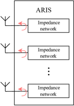
From (4), we may note that the RIS restriction, which can be written as $|\alpha_{i}|=1$, is now relaxed to $|\alpha_{i}|^{2}\leq 1$. The restriction $|\alpha_{i}|^{2}\leq 1$ comes from considering fully-reconfigurable passive (impedance) networks. However, it could further be removed by incuding active elements, e.g., amplifiers—as proposed in [34, 35]—which leads to the ARIS with relaxed power constraint. A potential implementation of ARIS is illustrated in Fig. 1(a).

Another RS model that has been studied in the literature is BD-RIS [31, 32], which extends the idea of RIS by allowing to interconnect different RS elements through a reconfigurable passive (impedance) network. The correspondence between the impendance network interconnecting the RS elements, and the resulting reflection matrix is one-to-one, and obtained from microwave network theory [36] as

$$\boldsymbol{\Theta}=(\boldsymbol{Z}+\mathbf{I}_{N})^{-1}(\boldsymbol{Z}-\mathbf{I}_{N}),$$ (5)

where $\boldsymbol{Z}$ is the $N\times N$ impedance matrix. Hence, the restrictions on the reflection matrix when considering different BD-RIS architectures are directly determined by the restrictions on the impendance network leading to $\boldsymbol{Z}$ [31]. In the case of ARIS, which corresponds to a restricted BD-RIS, no interconnection is assumed between elements, leading to a N-port network with diagonal impedance matrix, which correspondingly gives a diagonal reflection matrix. The power constraint $|\alpha_{i}|^{2}\leq 1$ further comes from the fact that, in passive (impedance) networks, the resistive part can only be positive. In the general case, a passive network has an impedance matrix with non-negative eigenvalues, i.e., the corresponding reflection matrix has eigenvalues smaller or equal to 1 [36, 31]. Moreover, assuming reciprocal networks—e.g., pure impedance networks—the impedance matrix has the extra restriction that it is symmetric, which further leads to a symmetric constraint in the reflection matrix, i.e., $\boldsymbol{\Theta}=\boldsymbol{\Theta}^{\text{T}}$.

As happened with the RIS case, most of the literature on BD-RIS [31, 32] focuses on the lossless case, i.e., where all the incident power at the BD-RIS is being reflected. However, it may still be interesting, under certain scenarios, to sacrifice some reflected power at the BD-RIS for improving other channel properties. Hence, we will consider a generalization over the common BD-RIS [31, 32] reflection model by assuming that the impedance network may include resistive (lossy) components instead of purely reactive (lossless) components. This leads to the following definition.

Definition 2

Beyond diagonal reconfigurable surface (BD-RIS) is hereby defined as an RS model whose reflection matrix satisfies

$$\boldsymbol{\Theta}_{\text{BD-RIS}}\in\{\boldsymbol{\Theta}\in\mathbb{C}^{N\times N}\;|\;\boldsymbol{\Theta}=\boldsymbol{\Theta}^{\text{T}},\,\|\boldsymbol{\Theta}\|^{2}_{2}\leq 1\},$$ (6)

where $\|\cdot\|_{2}$ corresponds to the matrix spectral norm. A BD-RIS with relaxed power constraint corresponds to a BD-RIS where the restriction $\|\boldsymbol{\Theta}\|^{2}_{2}\leq 1$ is disregarded.

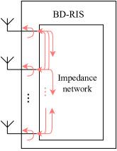
Assuming a fully reconfigurable impedance network, an arbitrary reflection matrix fulfilling (6) may be achieved by selecting the converse impedance matrix from (5). A potential implementation of BD-RIS is illustrated in Fig. 1(b). A more thorough discussion on specific implementations of the considered impedance networks is given in [32].

We also consider an RS model corresponding to a further generalization of the previous models.

Definition 3

Fully-reconfigurable intelligent surface (FRIS) is hereby defined as an RS model whose reflection matrix satisfies

$$\boldsymbol{\Theta}_{\text{FRIS}}\in\{\boldsymbol{\Theta}\in\mathbb{C}^{N\times N}\;|\;\|\boldsymbol{\Theta}\|^{2}_{2}\leq 1\}.$$ (7)

A FRIS with relaxed power constraint corresponds to a FRIS where the restriction $\|\boldsymbol{\Theta}\|^{2}_{2}\leq 1$ is disregarded.fn:amp

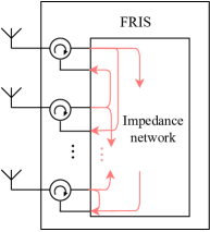
The practicality of FRIS is doubtful, but it naturally arises as a limit case for upper bounding the capabilities of RS systems. In fact, this type of RS gives the capacity achieving reflection matrix in [33], where the non-symmetric reflection matrix is further restricted to be unitary, corresponding again to the lossless case, i.e., reflecting maximum power. In principle, a general reflection matrix, as given by (7), may be achieved by considering a passive non-reciprocal network, i.e., including elements such as passive circulators or isolators [37]. In Fig. 1(c) we illustrate a possible implementation based on circulators, where the impedance network has now $2N$ ports instead of $N$ as in the previous designs. Other possible implementations may use $N$ pairs of RS elements, half of them for receiving and the other half for transmitting, as well as isolators between both sides; however, such implementations may lead to a loss of channel reciprocity. In any case, the reader may take FRIS as a mere theoretical concept to understand the limits of RS systems.

II-B Note on the downlink scenario

Assuming channel reciprocity, the results presented in this work may be trivially extended to the downlink scenario. Note that the architectures illustrated in Fig. 1 would maintain the reciprocity of the channel for fixed RS configuration. Thus, the downlink channel would correspond to the transpose of the uplink channel, retaining the same enhanced qualities without the need for RS reconfiguration.

III RS Channel Orthogonalization

The main goal of this work is to employ the previously defined RS technology to enforce channel orthogonality in the spatial domain. This would allow to perfectly multiplex the symbols transmitted by the different UEs without interference, nor noise enhancement as in zero-forcing (ZF) schemes. Note that, due to the passive nature of RS, we may assume that the covariance of the noise vector is unaffected by the reconfigurable reflection. We next define what is meant by channel orthogonality in the spatial domain.

Definition 4

We hereby define an orthogonal channel as a wireless propagation channel leading to a channel matrix $\widetilde{\boldsymbol{H}}$ which corresponds to a scaled element of the Stiefeld manifold, i.e.,

$$\widetilde{\boldsymbol{H}}=\sqrt{\beta}\widetilde{\boldsymbol{U}},$$ (8)

where $\beta$ is a real positive scalar corresponding to the channel gain, and $\widetilde{\boldsymbol{U}}$ is an element of the Stiefel manifold $\mathcal{S}(M,K)$ such that $\widetilde{\boldsymbol{U}}^{\text{H}}\widetilde{\boldsymbol{U}}=\mathbf{I}_{K}$. In other words, $\widetilde{\boldsymbol{U}}$ corresponds to a semi-unitary matrix which may be constructed by taking $K$ columns of an $M\times M$ unitary matrix $\boldsymbol{U}\in\mathcal{U}(M)$.

Note that the previous definition leads to a channel matrix whose squared singular values are all equal to $\beta$. We could consider a less restrictive definition by allowing for different eigenvalues while maintaining the orthogonality constraint, e.g., multiplying from the right in (8) a $K\times K$ diagonal matrix. In fact, most of the results presented in this work have straightforward extension to that case. Nevertheless, we focus our exposition on orthogonal channels given by (8) for notation simplicity and due to some increased benefits explained next.

Orthogonal channels, as given by (8), are hugely desirable in MU-MIMO systems for several reasons [6]:

• Full multiplexing gain is available since all of the singular values of the channel matrix are non-zero.

• The waterfilling algorithm [5] is not needed for achieving capacity since all eigenvalues of the channel are equal.

• The sum-rate is equally distributed among the UEs since the orthogonal spatial streams have equal power.

• Simple linear equalization or precoding, namely MRC or MRT, achieves optimum performance, since it can exploit the orthogonal paths of the channel without the need for UE cooperation.

We will now study the requirements for the different RS models to achieve arbitrary channel matrices, and specifically, to achieve an arbitrary orthogonal channel. We will start by ignoring the RS power constraints for analytical tractability. Nevertheless, whenever the collection of channels $\boldsymbol{H}_{0}$, $\boldsymbol{H}_{1}$, and $\boldsymbol{H}_{2}$, as well as the desired channel $\widetilde{\boldsymbol{H}}$, allow for an RS configuration fulfilling the respective power constraint, the presented results will provide it. On the other hand, if said collection of channels leads to an RS configuration not fulfilling the power constraint, we will show in the next section how to employ the freedom in the orthogonality constraint to minimize the RS power such that it may be implemented using purely passive components. Moreover, in the case of having $\boldsymbol{H}_{0}\approx\boldsymbol{0}_{M\times K}$, e.g., when the direct channel suffers from severe blockage, we will see that the RS power constrains may be trivially fulfilled by sacrificing channel gain.

III-A FRIS

We start by considering the FRIS model since this should lead to the most fundamental limits on the ability to generate arbitrary (orthogonal) channels with RS technology. The following proposition provides the conditions for FRIS to be able to generate arbitrary (orthogonal) channels.

Proposition 1

Given an arbitrary direct channel $\boldsymbol{H}_{0}$, and arbitrary full-rank channel matrices $\boldsymbol{H}_{1}$ and $\boldsymbol{H}_{2}$, a FRIS with relaxed power constraint is able to generate an arbitrary channel $\widetilde{\boldsymbol{H}}\neq\boldsymbol{H}_{0}$, and specifically an arbitrary orthogonal channel given by (8), if and only if

$$N\geq\max(M,K).$$ (9)

Said channel $\widetilde{\boldsymbol{H}}$ is achieved by configuring the FRIS reflection matrix as

$$\boldsymbol{\Theta}_{\text{FRIS}}=\text{vec}^{-1}\big{(}\boldsymbol{\mathcal{H}}^{\dagger}\boldsymbol{c}\big{)},$$ (10)

where $\boldsymbol{\mathcal{H}}^{\dagger}$ corresponds to the right pseudoinverse of $\boldsymbol{\mathcal{H}}=(\boldsymbol{H}_{2}^{\text{T}}\otimes\boldsymbol{H}_{1})$, and $\boldsymbol{c}=\text{vec}(\widetilde{\boldsymbol{H}}-\boldsymbol{H}_{0})$. An alternative (more compact) expression may be given by

$$\boldsymbol{\Theta}_{\text{FRIS}}=\boldsymbol{H}_{1}^{\dagger}\big{(}\widetilde{\boldsymbol{H}}-\boldsymbol{\mathcal{H}}_{0}\big{)}\boldsymbol{H}_{2}^{\dagger},$$ (11)

where $\boldsymbol{H}_{1}^{\dagger}$ and $\boldsymbol{H}_{2}^{\dagger}$ correspond to the right and left pseudoinverses of $\boldsymbol{H}_{1}$ and $\boldsymbol{H}_{2}$, respectively.

Proof:

We want to study solutions to the matrix equation

$$\boldsymbol{H}_{0}+\boldsymbol{H}_{1}\boldsymbol{\Theta}\boldsymbol{H}_{2}=\widetilde{\boldsymbol{H}},$$ (12)

which corresponds to a linear system of equations where $\boldsymbol{\Theta}$ is the unrestricted $N\times N$ complex matrix of unknowns. If we move $\boldsymbol{H}_{0}$ to the right-hand side (RHS) and vectorize, we may express (12) as

$$\boldsymbol{\mathcal{H}}\,\text{vec}(\boldsymbol{\Theta})=\boldsymbol{c},$$ (13)

where $\boldsymbol{c}=\text{vec}(\widetilde{\boldsymbol{H}}-\boldsymbol{H}_{0})$ is a non-zero $MK$-sized vector (since $\widetilde{\boldsymbol{H}}\neq\boldsymbol{H}_{0}$), and $\boldsymbol{\mathcal{H}}=(\boldsymbol{H}_{2}^{\text{T}}\otimes\boldsymbol{H}_{1})$ is an $MK\times N^{2}$ matrix. From the properties of the Kronecker product [38], we can characterize the rank of $\boldsymbol{\mathcal{H}}$ as

$$\text{rank}(\boldsymbol{\mathcal{H}})=\text{rank}(\boldsymbol{H}_{2})\cdot\text{rank}(\boldsymbol{H}_{1}),$$ (14)

where, since $\boldsymbol{H}_{1}$ and $\boldsymbol{H}_{2}$ are full rank, we have that $\text{rank}(\boldsymbol{H}_{1})=\min(M,N)$ and $\text{rank}(\boldsymbol{H}_{2})=\min(K,N)$. On the other hand, by fundamental linear algebra arguments, a solution to (13) can be found if and only if $\text{rank}(\boldsymbol{\mathcal{H}})=M\cdot K$, which leads to the condition (9). Moreover, if a solution to (13) exists, it is given by

$$\text{vec}(\boldsymbol{\Theta})=\boldsymbol{\mathcal{H}}^{\dagger}\boldsymbol{c},$$ (15)

where $\boldsymbol{\mathcal{H}}^{\dagger}$ is the right pseudoinverse of $\boldsymbol{\mathcal{H}}$. Note that there may be multiple solutions since the pseudoinverse may include $(N^{2}-MK)$ columns arbitrarily selected from the null-space of $\boldsymbol{\mathcal{H}}$. After inverse vectorization we reach (10). Moreover, exploiting the property of the Kronecker product $(\boldsymbol{A}\otimes\boldsymbol{B})^{\dagger}=\boldsymbol{A}^{\dagger}\otimes\boldsymbol{B}^{\dagger}$ [38] leads to (11). ∎

Proposition 1 sets a requirement on $N$ to generate arbitrary channels using FRIS. However, as seen in the previous section, practical implementations of FRIS may actually employ an impedance network with $2N$ ports. We will find out that, in some cases, this consideration could make FRIS implementations more restrictive than BD-RIS implementations.

III-B BD-RIS

The following theorem delimits the capabilities of BD-RIS to achieve arbitrary (orthogonal) channels.

Theorem 1

Given an arbitrary direct channel $\boldsymbol{H}_{0}$, and randomly chosen channel matrices $\boldsymbol{H}_{1}$ and $\boldsymbol{H}_{2}$, a BD-RIS with relaxed power constraint is able to generate an arbitrary channel $\widetilde{\boldsymbol{H}}\neq\boldsymbol{H}_{0}$, and specifically an arbitrary orthogonal channel as given by (8), if and only if

$$N\geq M+K-1.$$ (16)

Furthermore, (16) is also a sufficient condition for arbitrary full-rank $\boldsymbol{H}_{1}$ and $\boldsymbol{H}_{2}$. Said channel $\widetilde{\boldsymbol{H}}$ is achieved by configuring the BD-RIS reflection matrix as

$$\boldsymbol{\Theta}_{\text{BD-RIS}}=\text{vec}^{-1}\Big{(}\big{(}\boldsymbol{K}^{(N,N)}+\mathbf{I}_{N^{2}}\big{)}\boldsymbol{Z}_{\text{U/L}}\big{(}\boldsymbol{\mathcal{H}}_{\text{U}}+\boldsymbol{\mathcal{H}}_{\text{L}}\big{)}^{\dagger}\boldsymbol{c}\Big{)}$$ (17)

where $\boldsymbol{K}^{(N,N)}$ is the commutation matrix for $N\times N$ matrices [39], $\boldsymbol{c}=\text{vec}(\widetilde{\boldsymbol{H}}-\boldsymbol{H}_{0})$, $\boldsymbol{\mathcal{H}}_{\text{U/L}}$ corresponds is an $N^{2}\times N(N+1)$ matrix constructed from the columns of $\boldsymbol{\mathcal{H}}$ from (10) associated to the upper/lower triangular elements after vectorization, and $\boldsymbol{Z}_{\text{U/L}}$ is an $N^{2}\times N(N+1)/2$ matrix that pads zeros in the entries associated to elements below/above the diagonal after inverse vectorization.

Proof:

See Appendix. ∎

We may now note that, if we consider a FRIS implementation requiring a $2N$-port impendance network (as illustrated in Fig. 1(c)), the minimum $N$ from (16) and (9) would translate into a stricter requirement in terms of impedance network ports for FRIS than for BD-RIS, giving an increase of $\max\big{(}M-K+1,K-M+1\big{)}$ ports. This may be understood by the fact that such FRIS implementation corresponds to a non-reciprocal version of a BD-RIS with $2N$ elements where the non-reciprocicity actually reduces the DoF. However, the reduction in antenna elements may still be desirable in some scenarios. On the other hand, from (16) we may also notice that, assuming $M>1$ and/or $K>1$, BD-RIS does not make perfect use of all the $N(N+1)/2$ free variables in $\boldsymbol{\Theta}_{\text{BD-RIS}}$ since it actually requires an excess of $\lceil(M^{2}-M+K^{2}-K)/2\rceil$ free variables to be able to solve the $MK$ unknowns associated to the channel update.

III-C ARIS

The following proposition particularizes the previous results to the ARIS restriction.

Proposition 2

Given an arbitrary direct channel $\boldsymbol{H}_{0}$, and randomly chosen channel matrices $\boldsymbol{H}_{1}$ and $\boldsymbol{H}_{2}$, an ARIS with relaxed power constraint is able to generate an arbitrary channel $\widetilde{\boldsymbol{H}}\neq\boldsymbol{H}_{0}$, and specifically an arbitrary orthogonal channel given by (8), if and only if

$$N\geq MK.$$ (18)

Said channel $\widetilde{\boldsymbol{H}}$ is achieved by selecting the ARIS reflection matrix as

$$\boldsymbol{\Theta}_{\text{ARIS}}=\text{diag}\big{(}\boldsymbol{\mathcal{H}}_{D}^{\dagger}\boldsymbol{c}\big{)},$$ (19)

where $\boldsymbol{c}=\text{vec}(\widetilde{\boldsymbol{H}}-\boldsymbol{H}_{0})$, and $\boldsymbol{\mathcal{H}}_{D}$ is an $MK\times N$ matrix constructed from the columns of $\boldsymbol{\mathcal{H}}$ from (10) associated to the diagonal elements after vectorization.

Proof:

We study the solutions to the equation

$$\boldsymbol{H}_{0}+\boldsymbol{H}_{1}\boldsymbol{\Theta}_{\text{D}}\boldsymbol{H}_{2}=\widetilde{\boldsymbol{H}},$$ (20)

where $\boldsymbol{\Theta}_{\text{D}}=\text{diag}(\boldsymbol{\alpha}_{\text{D}})$ for an $N$-sized vector of unknowns $\boldsymbol{\alpha}_{\text{D}}$. We may proceed by vectorizing as in the proof of Proposition 1, leading to

$$\boldsymbol{\mathcal{H}}_{\text{D}}\boldsymbol{\alpha}_{\text{D}}=\boldsymbol{c},$$ (21)

where $\boldsymbol{\mathcal{H}}_{\text{D}}$ is an $MK\times N$ matrix whose columns correspond to the columns of $\boldsymbol{\mathcal{H}}$ multiplying the diagonal elements of $\boldsymbol{\Theta}$ in (13). Since $\boldsymbol{c}=\text{vec}(\widetilde{\boldsymbol{H}}-\boldsymbol{H}_{0})$ is a non-zero vector, (21)—corresponding to a linear equation—is solvable if and only if $\text{rank}(\boldsymbol{\mathcal{H}}_{\text{D}})=MK$. Let us assume (9) since this is clearly a necessary condition for (20). For arbitrary full rank matrices $\boldsymbol{H}_{2}$ and $\boldsymbol{H}_{1}$, we have that $\text{rank}(\boldsymbol{\mathcal{H}})=MK$. On the other hand, if $\boldsymbol{H}_{2}$ and $\boldsymbol{H}_{1}$ are further randomly chosen, any selection of columns/rows from $\boldsymbol{\mathcal{H}}$ will also be full rank with probability 1. Hence, having a selection $\boldsymbol{\mathcal{H}}_{\text{D}}$ of rank $MK$ is equivalent to (18). The solution (19) is then trivially given by inverting $\boldsymbol{\mathcal{H}}_{\text{D}}$ in (21), and constructing the diagonal matrix.

∎

IV Orthogonal channel selection

In this section, we provide techniques for selecting suitable orthogonal channels, given by (8), such that the required reflection matrix fulfills the passive restrictions from (7), (6), and (4). In the previous section, we derived closed-form expressions for the reflection matrices required to obtain an arbitrary (orthogonal) channel with FRIS, ARIS, and BD-RIS, given in (10), (17), and (19), respectively. The idea now is to exploit the freedom in the orthogonality constraint to restrict the power of the reflection matrix such that no amplification is required at the respective RS models.

In the three RS models considered, the power constraint allowing for channel orthogonalization using only passive components may be expressed in terms of the spectral norm as

$$\|\boldsymbol{\Theta}_{r}\|^{2}_{2}\triangleq\max_{\boldsymbol{x}}\frac{\boldsymbol{x}^{\text{H}}\boldsymbol{\Theta}_{r}^{\text{H}}\boldsymbol{\Theta}_{r}\boldsymbol{x}}{\|\boldsymbol{x}\|^{2}_{2}}\leq 1,$$ (22)

where $r\in\{\text{FRIS},\text{BD-RIS},\text{ARIS}\}$, and $\boldsymbol{\Theta}_{r}$ may be obtained by substituting (8), in (10), (17), and (19). We may write $\boldsymbol{\Theta}_{r}$ as

$$\boldsymbol{\Theta}_{r}=\text{vec}^{-1}\Big{(}\widetilde{\boldsymbol{\mathcal{H}}}_{r}\big{(}\sqrt{\beta}\text{vec}(\widetilde{\boldsymbol{U}})-\text{vec}(\boldsymbol{H}_{0})\big{)}\Big{)},$$ (23)

where $\widetilde{\boldsymbol{\mathcal{H}}}_{r}$ is an $N^{2}\times MK$ full-rank matrix respectively given by

$$\widetilde{\boldsymbol{\mathcal{H}}}_{\text{FRIS}}=\boldsymbol{\mathcal{H}}^{\dagger}$$ (24a)

$$\widetilde{\boldsymbol{\mathcal{H}}}_{\text{BD-RIS}}=\big{(}\boldsymbol{K}^{(N,N)}+\mathbf{I}_{N^{2}}\big{)}\boldsymbol{Z}_{\text{U/L}}\big{(}\boldsymbol{\mathcal{H}}_{\text{U}}+\boldsymbol{\mathcal{H}}_{\text{L}}\big{)}^{\dagger}$$ (24b)

$$\widetilde{\boldsymbol{\mathcal{H}}}_{\text{ARIS}}=\boldsymbol{Z}_{\text{D}}\boldsymbol{\mathcal{H}}_{D}^{\dagger},$$ (24c)

with $\boldsymbol{Z}_{\text{D}}$ corresponding to an $N^{2}\times N$ matrix that pads zeros in the entries associated to the off-diagonal elements after vectorization—converse to $\boldsymbol{Z}_{\text{U/L}}$ for the upper/lower triangular elements. Note that, whenever $\boldsymbol{H}_{0}=\boldsymbol{0}$, the only term left in (23) scales with $\sqrt{\beta}$, so if the direct channel is blocked we can always find a value of $\beta$ such that (22) is fulfilled. However, we are also interested in having the channel gain $\beta$ as high as possible since it multiplies the post-processed signal-to-noise ratio (SNR) for each UE, i.e., leading to the Shannon capacity [40]. In general, if a given $\widetilde{\boldsymbol{U}}$ allows for some $\beta\geq 0$ such that (22) is fulfilled, then $\|\boldsymbol{\Theta}_{r}\|^{2}_{2}$ is an increasing function in $\beta\geq\beta_{0}$ for some $\beta_{0}\geq 0$, so it is desirable to increase $\beta$ until (22) is fulfilled with equality. We could thus formulate our problem as

$$\max_{\widetilde{\boldsymbol{U}}}\beta,\;\;\text{s.t. }\|\boldsymbol{\Theta}_{r}\|_{2}^{2}=1.$$ (25)

However, a given combination of parameters may not even allow for fulfilling the constraint (25). Hence, our proposed solution considers the initial problem of minimizing $\|\boldsymbol{\Theta}_{r}\|_{2}^{2}$ over $\beta$ and $\widetilde{\boldsymbol{U}}$, and use the result as a starting point for attempting to solve (25). In the rest of this section, we will use the general formulation of $\boldsymbol{\Theta}_{r}$ from (23) to be able to provide general results applicable to the three RS models under study. However, the fact that $\boldsymbol{Z}_{S}$ and $\boldsymbol{Z}_{U/L}$ have several zero columns, as well as the properties of the commutation matrix, allow for some improvement in computation efficiency for ARIS and BD-RIS which may be leveraged for the numerical results. In the case of FRIS, we could also consider the alternative expression for the reflection matrix given in (11) to improve this efficiency, but this requires the knowledge of $\boldsymbol{H}_{1}$ and $\boldsymbol{H}_{2}$ (up to a shared scalar). We will see that, unlike in [1] where the FRIS is allowed to transmit pilots, a passive FRIS only allows us to estimate $\boldsymbol{\mathcal{H}}$. However, Kronecker product decomposition methods [41] could be potentially employed on $\boldsymbol{\mathcal{H}}$ to obtain estimates of $\boldsymbol{H}_{1}$ and $\boldsymbol{H}_{2}$, up to shared scaling.

IV-A RS power minimization

The initial concern is to find if a combination of $\beta$ and $\widetilde{\boldsymbol{U}}$ such that (22) can be fulfilled. We may tackle this by minimizing $\|\boldsymbol{\Theta}_{r}\|^{2}_{2}$ with respect to $\widetilde{\boldsymbol{U}}$ and $\beta$ and checking if the minimum value fulfills said constraint. The spectral norm $\|\boldsymbol{\Theta}_{r}\|^{2}_{2}$, given by the largest singular value of $\boldsymbol{\Theta}_{r}$, is generally difficult to minimize. On the other hand, the Frobenius norm $\|\boldsymbol{\Theta}_{r}\|_{\text{F}}=\text{tr}(\boldsymbol{\Theta}_{r}^{\text{H}}\boldsymbol{\Theta}_{r})$ corresponds to an equivalent matrix norm which upper-bounds the spectral norm, so by minimizing the Frobenius norm we can also reduce the spectral norm to a great extent. Let us thus consider the problem of minimizing the Frobenius norm $\|\boldsymbol{\Theta}\|^{2}_{\text{F}}=\text{tr}(\boldsymbol{\Theta}^{\text{H}}\boldsymbol{\Theta})$, which coincides with the Euclidean norm for vectorized matrices.

Considering (23), the squared Frobenius norm of $\boldsymbol{\Theta}_{r}$ for $r\in\{\text{FRIS},\text{BD-RIS},\text{ARIS}\}$ may be expressed as

$$P_{r}^{\text{Fro}}(\sqrt{\beta},\widetilde{\boldsymbol{U}})\triangleq\|\boldsymbol{\Theta}_{r}\|^{2}_{\text{F}}=\beta g_{r}(\widetilde{\boldsymbol{U}})-2\sqrt{\beta}f_{r}(\widetilde{\boldsymbol{U}})+\kappa_{r},$$ (26)

where

$$g_{r}(\widetilde{\boldsymbol{U}})=\text{vec}(\widetilde{\boldsymbol{U}})^{\text{H}}\widetilde{\boldsymbol{\mathcal{H}}}^{\text{H}}_{r}\widetilde{\boldsymbol{\mathcal{H}}}_{r}\text{vec}(\widetilde{\boldsymbol{U}})$$ (27a)

$$f_{r}(\widetilde{\boldsymbol{U}})=\mathfrak{Re}\big{\{}\text{vec}(\widetilde{\boldsymbol{U}})^{\text{H}}\widetilde{\boldsymbol{\mathcal{H}}}^{\text{H}}_{r}\widetilde{\boldsymbol{\mathcal{H}}}_{r}\text{vec}(\boldsymbol{H}_{0})\big{\}}$$ (27b)

$$\kappa_{r}=\text{vec}(\boldsymbol{H}_{0})^{\text{H}}\widetilde{\boldsymbol{\mathcal{H}}}_{r}^{\text{H}}\widetilde{\boldsymbol{\mathcal{H}}}_{r}\text{vec}(\boldsymbol{H}_{0}),$$ (27c)

with $\widetilde{\boldsymbol{\mathcal{H}}}_{r}$ given in (24) for $r\in\{\text{FRIS, BD-RIS, ARIS}\}$. Note that $g_{r}(\widetilde{\boldsymbol{U}})$ and $\kappa_{r}$ are always positive, while $f_{r}(\widetilde{\boldsymbol{U}})$ can be made positive or negative through $\widetilde{\boldsymbol{U}}$. The problem we want to solve may be formulated as

$$\arg\min_{\sqrt{\beta},\widetilde{\boldsymbol{U}}} \;P_{r}^{\text{Fro}}(\sqrt{\beta},\widetilde{\boldsymbol{U}})$$ (28)

s.t. $$\;\widetilde{\boldsymbol{U}}^{\text{H}}\widetilde{\boldsymbol{U}}=\mathbf{I}_{K}.$$

Since this problem is quadratic in $\sqrt{\beta}$, the optimal value for given $\widetilde{\boldsymbol{U}}$ corresponds to the stationary point

$$\sqrt{\beta_{\text{opt}}(\widetilde{\boldsymbol{U}})}=\frac{f_{r}(\widetilde{\boldsymbol{U}})}{g_{r}(\widetilde{\boldsymbol{U}})},$$ (29)

where we may assume that $\sqrt{\beta_{\text{opt}}(\widetilde{\boldsymbol{U}})}$ is positive since, from (27), the sign of $f_{r}(\widetilde{\boldsymbol{U}})$ can be absorbed in $\widetilde{\boldsymbol{U}}$ without loss of generality (WLOG). After substituting $\sqrt{\beta_{\text{opt}}(\widetilde{\boldsymbol{U}})}$ in (26) we get the equivalent problem

$$\arg\max_{\widetilde{\boldsymbol{U}}} \;\frac{f_{r}^{2}(\widetilde{\boldsymbol{U}})}{g_{r}(\widetilde{\boldsymbol{U}})}$$ (30)

s.t. $$\;\widetilde{\boldsymbol{U}}^{\text{H}}\widetilde{\boldsymbol{U}}=\mathbf{I}_{K}.$$

The previous maximization problem is generally non-convex. However, we may reach a local minimum by considering gradient ascent algorithms in the unitary group, as those proposed in [42]. To this end, we first need to characterize the gradient of the objective function in (30), given by

$$\boldsymbol{\Gamma}(\widetilde{\boldsymbol{U}})\triangleq\left(\frac{f_{r}^{2}(\widetilde{\boldsymbol{U}})}{g_{r}(\widetilde{\boldsymbol{U}})}\right)^{\prime}\!\!=\frac{2f_{r}(\widetilde{\boldsymbol{U}})g_{r}(\widetilde{\boldsymbol{U}})f_{r}^{\prime}(\widetilde{\boldsymbol{U}})-f_{r}^{2}(\widetilde{\boldsymbol{U}})g_{r}^{\prime}(\widetilde{\boldsymbol{U}})}{g_{r}^{2}(\widetilde{\boldsymbol{U}})},$$ (31)

where we have

$$f_{r}^{\prime}(\widetilde{\boldsymbol{U}})\triangleq\frac{\partial f_{r}(\widetilde{\boldsymbol{U}})}{\partial\widetilde{\boldsymbol{U}}^{*}}=\text{vec}^{-1}\big{(}\widetilde{\boldsymbol{\mathcal{H}}}^{\text{H}}_{r}\widetilde{\boldsymbol{\mathcal{H}}}_{r}\text{vec}(\boldsymbol{H}_{0})\big{)}$$ (32a)

$$g_{r}^{\prime}(\widetilde{\boldsymbol{U}})\triangleq\frac{\partial g_{r}(\widetilde{\boldsymbol{U}})}{\partial\widetilde{\boldsymbol{U}}^{*}}=\text{vec}^{-1}\big{(}\widetilde{\boldsymbol{\mathcal{H}}}^{\text{H}}_{r}\widetilde{\boldsymbol{\mathcal{H}}}_{r}\text{vec}(\widetilde{\boldsymbol{U}})\big{)}.$$ (32b)

We may then employ the algorithm from [42, Table II], which consists of computing the Riemannian gradient, and computing the gradient update using the geodesic equation. The algorithm in [42, Table II] further considers the use of Armijo line search for computing the the step size, which assures better convergence (the algorithm will converge almost surely to a local minimum [43]).

We further propose a closed-form heuristic selection of $\widetilde{\boldsymbol{U}}$ to decrease $\|\boldsymbol{\Theta}_{r}(\widetilde{\boldsymbol{U}})\|^{2}_{\text{F}}$ which may be used as a starting point for (30). If we take a look at (23), ignoring the inverse vectorization, we note that we have a product of two terms. The first term is matrix determined by the cascaded channel, and the second term corresponds to the difference between the direct channel and the desired channel. In light of this, we may consider a strategy of choosing the direct channel such that the second term falls close to the lowest eigenmode of the first term. Note that, in the unrestricted case, fixing the second term such that it falls precisely in the lowest eigenmode leads to the optimal selection for given norm. Considering the orthogonal desired channel constraint, we may select

$$\widetilde{\boldsymbol{U}}=\mathcal{P}_{\mathcal{S}(M,K)}\Big{(}\text{vec}^{-1}\big{(}\boldsymbol{v}_{r,MK}+\text{vec}(\boldsymbol{H}_{0})\big{)}\Big{)},$$ (33)

where $\boldsymbol{v}_{r,MK}$ is the right unitary vector of $\boldsymbol{\mathcal{H}}_{r}$ associated to the lowest singular value, and $\mathcal{P}_{\mathcal{S}(M,K)}(\cdot)$ is the projection under any unitarily invariant norm—e.g., Frobenius and spectral norm—onto the Stiefel manifold $\mathcal{S}(M,K)$ given by [44]

$$\mathcal{P}_{\mathcal{S}(M,K)}(\boldsymbol{A})=\boldsymbol{U}_{\boldsymbol{A}}\begin{bmatrix}\mathbf{I}_{K}\\ \boldsymbol{0}\end{bmatrix}\boldsymbol{V}_{\boldsymbol{A}}^{\text{H}},$$ (34)

where $\boldsymbol{U}_{\boldsymbol{A}}$ and $\boldsymbol{V}_{\boldsymbol{A}}^{\text{H}}$ are the left and right unitary matrices of the singular value decomposition of the arbitrary $M\times K$ matrix $\boldsymbol{A}$. Note that $\mathcal{P}_{\mathcal{S}(M,K)}(\boldsymbol{A})$ corresponds to the rotation matrix associated to the polar decomposition of $\boldsymbol{A}$ [45]. If the direct channel $\boldsymbol{H}_{0}$ is dominant over $\boldsymbol{v}_{r,MK}$, the selection will favor minimizing the distance between the desired orthogonal channel and the direct channel, whereas, if the direct channel is strongly blocked, the selection will favor minimizing the distance between the desired orthogonal channel and the lowest eigenmode of $\boldsymbol{\mathcal{H}}_{r}$.

IV-B Channel gain maximization

As previously mentioned, we are interested in having the channel gain $\beta$ as high as possible since it has direct impact on the rate at which each of the UEs may transmit data. Hence, assuming that we can find $\beta$ and $\widetilde{\boldsymbol{U}}$ such that (22) is fulfilled—e.g., by using the proposed approximate solutions to (28)—the next aim is to maximize $\beta$ by trying to solve (25).

Let us assume that we can find $\widetilde{\boldsymbol{U}}_{0}$ such that, for some $\beta_{0}\geq\beta_{\text{opt}}(\widetilde{\boldsymbol{U}}_{0})$ from (29), we get a reflection matrix fulfilling (22) with strict inequality, i.e., $\|\boldsymbol{\Theta}_{r}\|^{2}_{2}<1$. Due to the characteristics of the spectral norm, it is not obvious how much $\beta$ can be increased until (22) is fulfilled with equality. The reason is that the vector $\boldsymbol{x}$ in (22), which we may assume to be a unit vector WLOG, is dependent on $\beta$. To solve this problem, we propose an iterative procedure where, starting with $\beta_{0}$, we alternate between obtaining the unit vector $\boldsymbol{x}_{i}$ solving the maximization in (22) for the current $\beta_{i}$, and obtaining the highest $\beta_{i+1}$ such that $\boldsymbol{x}^{\text{H}}_{i}\boldsymbol{\Theta}_{r}(\beta_{i+1})^{\text{H}}\boldsymbol{\Theta}_{r}(\beta_{i+1})\boldsymbol{x}_{i}=1$, which corresponds to solving a quadratic equation in $\sqrt{\beta_{i+1}}$. The convergence of this method is assured by observing that $\{\|\boldsymbol{\Theta}_{r}(\beta_{i})\|^{2}_{2}\}_{i\geq 1}$ is a decreasing sequence lower bounded by $1$, while we know there exists $\beta_{0}$ such that $\|\boldsymbol{\Theta}_{r}(\beta_{0})\|^{2}_{2}<1$. Hence, $\|\boldsymbol{\Theta}_{r}(\beta_{i})\|^{2}_{2}$ will converge to 1, and $\beta_{i}$ will converge to the maximum value allowing for $\|\boldsymbol{\Theta}_{r}(\beta_{i})\|^{2}_{2}=1$ with the given $\widetilde{\boldsymbol{U}}=\widetilde{\boldsymbol{U}}_{0}$.

We have presented a rule for adjusting $\beta$ such that (22) is fulfilled with equality. We can further try to solve (25) by iteratively minimizing $\|\boldsymbol{\Theta}_{r}(\widetilde{\boldsymbol{U}})|_{\beta=\beta_{i}}\|^{2}_{2}$ over $\widetilde{\boldsymbol{U}}$, and use the previous method to increment $\beta$ until $\|\boldsymbol{\Theta}_{r}(\beta_{i})|_{\widetilde{\boldsymbol{U}}=\widetilde{\boldsymbol{U}}_{i}}\|^{2}_{2}=1$. Assuming we can find the global minimizer $\widetilde{\boldsymbol{U}}_{i}$ of $\|\boldsymbol{\Theta}_{r}(\widetilde{\boldsymbol{U}})|_{\beta=\beta_{i}}\|^{2}_{2}$ at iteration $i$, this method will converge to the optimal solution of (25), since in each iteration $\beta$ is increased and upper bounded by the finite optimal value. However, finding a global minimizer $\widetilde{\boldsymbol{U}}_{i}$ of $\|\boldsymbol{\Theta}_{r}(\widetilde{\boldsymbol{U}})|_{\beta=\beta_{i}}\|^{2}_{2}$ is non-trivial. We thus consider approximate solutions by solving the alternative problem given in (28) for fixed $\beta$, which only differs from (28) in that $\beta$ is constant and not treated as an optimization variable. This can be done by using methods for minimization with unitary constraints as the ones considered for solving (30). Specifically, we consider again the algorithm from [42, Table II], where the gradient of the objective function is now given by

$$\boldsymbol{\Gamma}_{\beta}(\widetilde{\boldsymbol{U}})\triangleq\frac{\partial P_{r}^{\text{Fro}}(\sqrt{\beta},\widetilde{\boldsymbol{U}})}{\partial\widetilde{\boldsymbol{U}}}=\beta g_{r}^{\prime}(\widetilde{\boldsymbol{U}})-2\sqrt{\beta}f_{r}^{\prime}(\widetilde{\boldsymbol{U}}),$$ (35)

where $g_{r}^{\prime}(\widetilde{\boldsymbol{U}})$ and $f_{r}^{\prime}(\widetilde{\boldsymbol{U}})$ are given in (32).

Algorithm 1 summarizes the proposed method for orthogonal channel selection. We have used the notation $\boldsymbol{v}_{\max}(\cdot)$ to denote an eigenvector associated to the largest eigenvalue of the positive semi-definite input matrix. We will also consider a simplified version of Algorithm 1 where we skip step 10, since the use of [42, Table II] may lead to large computation times due to the variability in convergence speed.

Algorithm 1 Orthogonal channel selection algorithm.

0:  $\boldsymbol{H}_{0}$, $\widetilde{\boldsymbol{\mathcal{H}}}_{r}$

0:  $\beta$, $\widetilde{\boldsymbol{U}}$ RS power minimization :

1:  Select initial $\widetilde{\boldsymbol{U}}$ and $\beta$, e.g., by (33) and (29).

2:  if $\|\boldsymbol{\Theta}_{r}\|^{2}_{2}>1$ then

3:     Use [42, Table II] to find $\widetilde{\boldsymbol{U}}$ maximizing (30)

4:     $\beta\leftarrow$ Update with (29)

5:     if $\|\boldsymbol{\Theta}_{r}\|^{2}_{2}>1$ then

6:        Active amplification may be required

7:     end if

8:  end ifChannel gain maximization :

9:  while $\beta$ has not converged do

10:     Use [42, Table II] to find $\widetilde{\boldsymbol{U}}$ minimizing (22) (fixed $\beta$)

11:     while $\beta$ has not converged do

12:        $\boldsymbol{x}=\boldsymbol{v}_{\max}\big{(}\boldsymbol{\Theta}_{r}^{\text{H}}(\beta)\boldsymbol{\Theta}_{r}(\beta)\big{)}$

13:        $\sqrt{\beta}\leftarrow$ Largest root of $\boldsymbol{x}^{\text{H}}\boldsymbol{\Theta}_{r}^{\text{H}}(\beta)\boldsymbol{\Theta}_{r}(\beta)\boldsymbol{x}-1$

14:     end while

15:  end while

V Channel estimation and RS configuration

We now turn our focus into proposing efficient techniques to estimate the channel coefficients required to be able to apply the respective configuration within the different RS models considered. The aim is to obtain the necessary parameters to be able to perform channel selection and RS configuration. In (23), we have a general expression for the desired reflection matrix of the RS technologies under study. We thus need to estimate the channel parameters that allow to characterize $\widetilde{\boldsymbol{\mathcal{H}}}_{r}$ and $\boldsymbol{H}_{0}$, which are the only parameters employed in the computation of the channel selection and RS configuration. From (24), the required channel parameters are given by $\boldsymbol{\mathcal{H}}$, $(\boldsymbol{\mathcal{H}}_{\text{U}}+\boldsymbol{\mathcal{H}}_{\text{L}})$, and $\boldsymbol{\mathcal{H}}_{\text{S}}$ for FRIS, BD-RIS, and ARIS, respectively. Note that, $(\boldsymbol{\mathcal{H}}_{\text{U}}+\boldsymbol{\mathcal{H}}_{\text{L}})$ and $\boldsymbol{\mathcal{H}}_{\text{S}}$ correspond to reduced matrices coming from $\boldsymbol{\mathcal{H}}$ by selecting and/or combining columns, so BD-RIS and ARIS may be seen as a special case of FRIS with restricted channel knowledge.

Due to the passive (energy-efficient) nature of RS technology[46, 47], we assume that, during the training phase, the estimation/computation tasks are carried out at the BS, while the RS only needs to configure its impedance networks by following a preprogrammed training sequence. Once the RS configuration is computed at the BS, it is then forwarded to the RS which may then implement it by tuning its impedance networks accordingly. We also assume that the desired channel is conveniently selected at the BS—e.g., through the proposed channel selection algorithm—so that it can use it in the data phase for decoding/precoding purposes without the need for extra channel estimation steps. Next, we describe the proposed estimation and configuration scheme consisting of three stages: direct channel estimation, cascaded channel coefficients estimation, and RS configuration.

V-A Direct Channel Estimation

Assuming the direct channel $\boldsymbol{H}_{0}$ is not blocked, all the considered RS models require full knowledge of said channel. Hence, in the initial step the RS would configure its reflection matrix $\boldsymbol{\Theta}=\boldsymbol{0}$, which is allowed in the FRIS, ARIS, and BD-RIS models. This corresponds to configuring the impedance networks such that all the impinging power is dissipated in the RS resistive components. A practical alternative in more restricted RS models is to reflect the power in a direction away from the BS—i.e., putting $\boldsymbol{\Theta}$ in the null-space of $\boldsymbol{H}_{1}$ and/or $\boldsymbol{H}_{2}$—or to use a two step-method with reflection matrices $\boldsymbol{\Theta}_{1}$ and $\boldsymbol{\Theta}_{2}$ such that $\boldsymbol{\Theta}_{1}+\boldsymbol{\Theta}_{2}=\boldsymbol{0}$. Assuming $\boldsymbol{\Theta}=\boldsymbol{0}$ is effectively achieved, the UEs may send a sequence of $K$ orthogonal pilots to estimate $\boldsymbol{H}_{0}$. The received signal over the $K$ time slots is a $K\times K$ matrix given by

$$\boldsymbol{Y}_{0}=\boldsymbol{H}_{0}\boldsymbol{P}+\boldsymbol{N}_{0},$$ (36)

where $\boldsymbol{P}$ is the $K\times K$ known pilot matrix fulfilling $\boldsymbol{P}\boldsymbol{P}^{\text{H}}=E_{s}\mathbf{I}_{K}$, and $\boldsymbol{N}_{0}$ is the noise matrix with IID entries $\{\boldsymbol{N}_{0}\}_{i,j}\sim\mathcal{CN}(0,N_{0})$. We can then estimate $\boldsymbol{H}_{0}$ by removing the pilot matrix, i.e., multiplying $1/E_{s}\boldsymbol{P}^{\text{H}}$ from the right, which would not affect the distribution of the estimation noise except for the corresponding scaling.

V-B Cascaded Channel Coefficients Estimation

We proceed with the estimation of the required cascaded channel coefficients, associated to matrix $\widetilde{\boldsymbol{\mathcal{H}}}_{r}$ from (24). In general, it is enough to perform the estimation of the cascaded channel coefficients obtained from a sequence of configurations of the reflection matrix $\boldsymbol{\Theta}$ forming a basis for the vector spaces defined by its constraints—given in (7), (6), and (4) for the different RS models—since this would capture enough parameters to exploit the DoFs of the RS reflection. This can be understood by looking at the linear equation (13), which captures the ability of FRIS to configure the channel, and where the particularization to BD-RIS and ARIS corresponds to imposing the extra constraints on $\text{vec}(\boldsymbol{\Theta})$. We will exemplify how this process looks like by considering a simple basis for each the three RS models under study, but extension to other bases is trivial.

V-B1 FRIS

This corresponds to the most general case since $\boldsymbol{\Theta}_{\text{FRIS}}$ is unrestricted (except for the power constraint). However, all the columns of $\boldsymbol{\mathcal{H}}$ have to be estimated to be able to exploit the full capabilities of FRIS. We would thus need a sequence of $N^{2}$ steps, where in step $n$ the FRIS selects $\boldsymbol{\Theta}=\boldsymbol{E}_{i_{n},j_{n}}$, with $i_{n}$ and $j_{n}$ corresponding to the indexes such that $\text{vec}(\boldsymbol{\Theta})$ has its non-zero entry at position $n$—leading to the canonical basis for $\text{vec}(\boldsymbol{\Theta})$. At each step, the UEs would send $K$ orthogonal pilots, leading to the following received matrix at step $n$

$$\boldsymbol{Y}_{n}=\boldsymbol{H}_{0}\boldsymbol{P}+\boldsymbol{h}_{1i_{n}}\boldsymbol{h}_{2j_{n}}^{T}\boldsymbol{P}+\boldsymbol{N}_{n},$$ (37)

where $\boldsymbol{h}_{1i_{n}}$ is the $i_{n}$th column of $\boldsymbol{H}_{1}$, $\boldsymbol{h}_{2j_{n}}^{\text{T}}$ is the $j_{n}$th row of $\boldsymbol{H}_{2}$, and $\boldsymbol{N}_{n}$ is the corresponding IID Gaussian noise matrix. In (37), we can remove the pilot matrix as before and subtract our estimate of $\boldsymbol{H}_{0}$ from the previous stage, leading to an estimate of $\boldsymbol{h}_{1i_{n}}\boldsymbol{h}_{2j_{n}}^{T}$ with IID Gaussian estimation noise (since we have just applied unitary transformations and combined IID Gaussian matrices). We may note that $\text{vec}(\boldsymbol{h}_{1i_{n}}\boldsymbol{h}_{2j_{n}}^{T})$ corresponds to the $n$th column of $\boldsymbol{\mathcal{H}}$, so, after repeating the process for the sequence of $N^{2}$ base configurations, we would reach an estimate of the whole $\boldsymbol{\mathcal{H}}$.

V-B2 BD-RIS

The constraint on $\boldsymbol{\Theta}$ of being symmetric now translates into having only $N(N+1)/2$ free variables—$\text{vec}(\boldsymbol{\Theta})$ in (13) would have $N(N-1)/2$ repeated entries. We can proceed as in the FRIS case, but we would now have $N(N+1)/2$ steps, where in step $n$ we may configure the RS with reflection matrix $\boldsymbol{\Theta}=\boldsymbol{E}_{i_{n},j_{n}}+\boldsymbol{E}_{j_{n},i_{n}}$, generating an orthonormal basis for the space of $N\times N$ symmetric matrices. Again, other less sparse bases may be more desirable to avoid receiver sensitivity issues, but this basis gives a convenient example. The received matrix over $K$ orthogonal pilot slots can now be written as

$$\boldsymbol{Y}_{n}=\boldsymbol{H}_{0}\boldsymbol{P}+\boldsymbol{h}_{1i_{n}}\boldsymbol{h}_{2j_{n}}^{T}\boldsymbol{P}+\boldsymbol{h}_{1j_{n}}\boldsymbol{h}_{2i_{n}}^{T}\boldsymbol{P}+\boldsymbol{N}_{n}.$$ (38)

Following the same reasoning as for FRIS, we may reach an estimate of $\boldsymbol{h}_{1i_{n}}\boldsymbol{h}_{2j_{n}}^{T}+\boldsymbol{h}_{1j_{n}}\boldsymbol{h}_{2i_{n}}^{T}$ with IID Gaussian estimation noise. The vectorization of said estimated matrix corresponds to the $n$th column of $(\boldsymbol{\mathcal{H}}_{\text{U}}+\boldsymbol{\mathcal{H}}_{\text{L}})$, so after $N(N+1)/2$ we would have estimated all the channel coefficients required to configure the BD-RIS.

V-B3 ARIS

The constraint now is that $\boldsymbol{\Theta}$ has to be diagonal. This means that $\text{vec}(\boldsymbol{\Theta})$ in (13) has only $N$ non zero elements multiplying the respective columns of $\boldsymbol{\mathcal{H}}$. We may then follow the same steps as in FRIS, but configuring $\boldsymbol{\Theta}=\boldsymbol{E}_{n,n}$ at step $n$—generating an orthonormal basis for the space of $N\times N$ diagonal matrices. Following the same reasoning as in FRIS, we may get an estimate of $\boldsymbol{h}_{1n}\boldsymbol{h}_{2n}^{T}$, which corresponds to the $n$th column of $\boldsymbol{\mathcal{H}}_{\text{S}}$ in (19). Hence, after $N$ steps we have estimated all the necessary channel coefficients to configure the ARIS, where the estimation noise is again IID Gaussian.

If we select the minimum $N$ in the different RS models—i.e., fulfilling with equality (9), (16), and (18), respectively—we obtain the minimum number of pilot slots of length $K$ required to estimate the cascaded channel channel parameters, given by $L_{\text{ARIS}}=MK$, $L_{\text{FRIS}}=\min(M,K)^{2}$, and $L_{\text{BD-RIS}}=(M+K-1)(M+K-2)/2$. We can note that for $M\neq K$ we always have $L_{\text{FRIS}}<\min(L_{\text{ARIS}},L_{\text{BD-RIS}})$, showcasing another limitation in terms of FRIS practicality. On the other hand, the comparison between $L_{\text{ARIS}}$ and $L_{\text{BD-RIS}}$ is dependent on $M$ and $K$, but for large enough $M$ (or $K$) $L_{\text{BD-RIS}}$ will be larger due to its quadratic relation to $M$ (and $K$).

V-C RS Configuration

After having estimated the necessary channel parameters to configure the respective RS models, the BS can select a suitable desired channel, e.g., an orthogonal channel with high gain that does not require RS amplification. The BS may hereby employ Algorithm 1 for channel selection, which requires only knowledge of the estimated channel parameters—from which we can obtain estimates of $\widetilde{\boldsymbol{\mathcal{H}}}_{r}$ and $\boldsymbol{H}_{0}$. Then, the BS can compute the reflection matrix to be applied at the RS for achieving said channel. The reflection matrix for FRIS, BD-RIS, and ARIS may be computed by using equations (10), (17), and (19), respectively. We may further translate the respective reflection matrices into impedance network parameters by considering (5).

VI Numerical results and examples

VI-A Performance under IID Rayleigh fading

We first analyze the performance of Algorithm 1, as well as its simplified version when $\widetilde{\boldsymbol{U}}$ is directly fixed to (33) and [42, Table 2] is disregarded. We have considered a rich multipath propagation environment where $\boldsymbol{H}_{0}$, $\boldsymbol{H}_{1}$, and $\boldsymbol{H}_{2}$ may be modelled as IID Gaussian matrices [6]. From the theoretical results in Section IV, the ratio between power of the direct channel and the power of the cascaded channel seems to be a limiting factor towards perform channel orthogonalization. We have thus considered different values for this ratio by fixing the average power of the cascaded channel entries to 1, i.e., $\mathbb{E}\big{\{}|\{\boldsymbol{H}_{1}\}_{i,j}|^{2}\big{\}}=1$ and $\mathbb{E}\big{\{}|\{\boldsymbol{H}_{2}\}_{i,j}|^{2}\big{\}}=1$, and selecting $\eta$ as the power of the direct channel elements, i.e., $\big{\{}|\{\boldsymbol{H}_{0}\}_{i,j}|^{2}\big{\}}=\eta$, which allows to control said ratio.

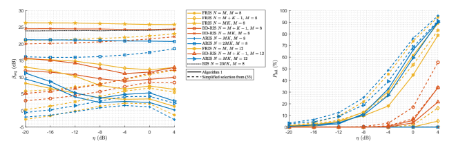
In Fig. 2 (left) we plot the average channel gain over $10^{3}$ channel realizations, $\beta_{\text{avg}}$, versus $\eta$ in a $K=4$ UEs scenario, where we consider various configurations of BS antennas and RS antennas. Note that the value of $\beta$ is directly related to the Shannon capacity of each UE through $\log(1+\beta\text{SNR})$ [40]. We have pessimistically assumed that the channel gain is 0 for every channel realization where the channel selection has failed to provide a solution fulfilling the respective RS passive constraint. Moreover, we have limited the number of iterations of the while loops from [42, Table 2] to avoid unreasonable computation times when the convergence is too slow at the cost of limiting the optimality of the results. As expected, for the same number of RS elements, FRIS outperforms BD-RIS, which outperforms ARIS by a wider margin. However, when selecting the minimum number of RS elements from (18), (16), and (9), FRIS and ARIS achieve a similar channel gain, while BD-RIS can get a substatial improvement (reaching over 10 dB gain for some values of $\eta$). We may also observe that an increase in the number of BS antennas effectively leads to a shift in $\beta_{\text{avg}}$, where the shift seems to be larger for larger RS freedom, i.e., FRIS has greater benefit from more BS antennas than BD-RIS, which has greater benefit than ARIS. On the other hand, the simplified channel selection seems to perform closer to Algorithm 1 as the power of the direct channel increases, meaning that it does a better job at trying to compensate the direct channel than in projecting the solution towards the lowest eigenmode of $\boldsymbol{\mathcal{H}}_{r}$. We have included for comparison the average channel gain for a RIS scenario with $M=8$ and $N=2MK$ elements—same as the best performing ARIS selection. The RIS phases have been optitimized using numerical solvers for maximizing the condition number of the channel, which gives a measure of the orthogonality of the channel [1]. Interestingly, by allowing a small error in the orthogonality constraint, RIS can actually achieve a better channel gain than ARIS with the same number of elements, since its model actually is fixed to reflect maximum power—BD-RIS and FRIS with the same $N$ still lead to a considerable improvement of 2-5 dB. A natural extension of this work could thus consider a relaxation of the orthogonality constraint to study the interplay between channel gain and level of orthogonality.

Fig. 2 (right) shows the failure rate $P_{\text{fail}}$, which is defined as the rate of channel realizations where the channel selection leads to a configuration not fulfilling the passive constraint—i.e., leading to $\beta=0$ in our previous simulation. The same considerations as for Fig. 2 (left) are taken regarding the channel model, employed methods, etc. As expected, the higher the direct channel power (with respect to the cascaded channel power) the higher the failure rate since more power is required to compensate this channel, increasing the minimum $\beta$ to do it—recall that $\sqrt{\beta}$ is quadratically related to the RS power. We may identify similar trends in performance as in the previous simulation results, but we now see that adding extra RS elements eventually leads to $0\%$ failure in the considered range, achieved in our results for ARIS with $N=2MK$, or for BD-RIS and FRIS with $N=MK$. Note that the RIS model is not applicable for this case since it always leads to non-zero orthogonality mismatch by enforcing the full-reflection constraint.

Figure 2: Average channel gain (left) and failure rate (right) versus direct channel power for MU-MIMO with $K=4$.

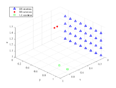
VI-B Pure LoS Example Scenario

We next analyze an example of a pure LoS scenario at 2.4 GHz to showcase the potential of channel orthogonalization with RS. The scenario is depicted in Fig. 3, where all the antenna elements are assumed isotropic, and free space propagation is assumed. In such scenario, by employing Algorithm 1, if the RS corresponds to a FRIS we reach a normalized channel gain of $5$ dB, while if the RS corresponds to a BD-RIS we get a normalized channel gain of $4.85$ dB. On the other hand, if the RS corresponds to an ARIS we are not able to find a suitable orthogonal channel that does not require amplification (the minimum amplification required is 7.42 dB). On the other hand, if the RS corresponds to a RIS maximizing condition number, the average channel gain is $3.84$ dB, while the minimum channel gain is just $1.93$ dB. The main challenge in this type of scenarios comes from the fact that the cascaded channel suffers from double path loss, leading to significantly higher power loss than in the direct channel. Hence, the pure LoS can be seen as a worst case scenario, while considering blockage in the direct channel, or including some multipath propagation would likely help to even up the ratio between direct and cascaded channel power.

Figure 3: LoS scenario.

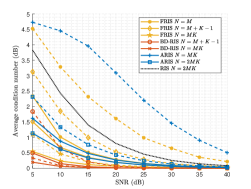
VI-C Imperfect CSI Scenario under IID Rayleigh fading

In Fig. 4 we study the effect of imperfect-CSI on the condition number of the orthogonalized channel with respect to SNR. We have based the simulations on the channel estimation procedure from Section V, which considers estimation over a single time-frequency resource–i.e., leading to correspondence between the estimation SNR and the communication SNR—but we could further increase the estimation SNR, e.g., by combining several time samples or highly-correlated subcarriers. We have also focused on the case where the direct channel is blocked, i.e., $\boldsymbol{H}_{0}=\boldsymbol{0}$, since the presence of an imperfect direct channel only leads to an extra addititive IID Gaussian noise term in the final channel, which has simple characterization, while the imperfect-CSI cascaded channel has less predictable impact due to the involvement of complex operations like matrix pseudoinverses. Moreover, $\boldsymbol{H}_{0}=\boldsymbol{0}$ assures that the RS models can fulfill the passive constraint in all cases whenever the respective conditions from (18), (16), and (9) are fulfilled. The simulation considers $10^{3}$ IID Gaussian realizations of $\boldsymbol{H}_{1}$ and $\boldsymbol{H}_{2}$ with normalized power, and we have compared a random orthogonal channel selection with a channel selection based on Algorithm 1. The results showcase how the proposed channel selection generally helps in reducing the effect of imperfect-CSI towards the loss of orthogonality, especially with excess of RS elements. Interestingly, BD-RIS outperforms FRIS even for the same number of elements, which can be understood by the fact that the FRIS configuration employs considerably more noisy channel parameters ($N^{2}$) than BD-RIS ($N(N+1)/2$). Moreover, all the results show improved orthogonalization performance than RIS—which has been again numerically optimized for minimum condition number—even for a lower number of elements.

Figure 4: Condition number under imperfect-CSI in MU-MIMO with $M=8$ and $K=4$.

VII Conclusions and Future Work

We have analysed the use passive RS technology for channel orthogonalization in MU-MIMO. We have presented three RS models which generalize the widely studied models, and we have discussed their potential implementation, as well as the respective restrictions on the achievable reflection matrices. We have also derived the conditions for achieving arbitrary (orthogonal) channel configuration with the considered RS models. Moreover, we have shown methods to optimize the channel selection procedure, and to practically estimate the channel parameters to be able to apply the corresponding RS configuration. The numerical results have showcased the potential of the methods presented, which allow for perfect channel orthogonalization with reduced loss in terms of channel gain. Overall, BD-RIS seems to achieve a good trade-off in terms of performance and complexity, but more research is needed to confirm its practicality.

The presented work takes an important step towards the achievement of OSDM, which has been proposed as the spatial converse to orthogonal time-frequency modulations like OFDM. However, these results constitute the beginning of a novel research direction with many possibilities of extension. For example, future work could consider the use of alternative technologies to RS in the task of channel orthogonalization. Regarding closer extension to the presented work, we could study the use of alternative optimization methods to those proposed in Section IV. For example, we could consider exploiting the freedom in the pseudoinverse to further improve the results, or we could try to adapt the results to the spectral norm instead of using the relaxation to Frobenius norm. Moreover, the imperfect CSI scenario could also be optimized by proposing specific channel selection schemes which take into account the distribution of the estimation error. Another interesting extension could consider studying the interplay between channel gain and level of orthogonality.

The presented results can also be employed to address other research questions. For example, these findings could be employed towards estimating the number of RIS elements required in general scenarios with different requirements. On the other hand, the general estimation procedure we studied can also be considered in such scenarios to understand the required pilot overhead.

[Proof of Theorem 1] We seek to study the solutions to the matrix equation

$$\boldsymbol{H}_{0}+\boldsymbol{H}_{1}\boldsymbol{\Theta}_{\text{S}}\boldsymbol{H}_{2}=\widetilde{\boldsymbol{H}},$$ (39)

where $\boldsymbol{\Theta}_{\text{S}}=\boldsymbol{\Theta}_{\text{S}}^{\text{T}}$ with dimension $N\times N$, and $\widetilde{\boldsymbol{H}}$ is a non-zero $M\times K$ matrix. We can define WLOG $\boldsymbol{\Theta}_{\text{S}}=\boldsymbol{\Theta}_{\text{U/L}}+\boldsymbol{\Theta}_{\text{U/L}}^{\text{T}}$, where $\boldsymbol{\Theta}_{\text{U/L}}$ corresponds to an upper/lower triangular matrix. We can then rewrite (39) as

$$\boldsymbol{H}_{1}\boldsymbol{\Theta}_{\text{U/L}}\boldsymbol{H}_{2}+\boldsymbol{H}_{1}\boldsymbol{\Theta}_{\text{U/L}}^{\text{T}}\boldsymbol{H}_{2}+\boldsymbol{H}_{0}=\widetilde{\boldsymbol{H}}.$$ (40)

After vectorizing, we reach the linear equation

$$(\boldsymbol{\mathcal{H}}+\boldsymbol{\mathcal{H}}\boldsymbol{K}^{(N,N)})\boldsymbol{Z}_{\text{U/L}}\boldsymbol{\phi}=\boldsymbol{c},$$ (41)

where $\boldsymbol{\phi}$ is a vector containing the unique unknowns from $\boldsymbol{\Theta}_{\text{S}}$ (with the diagonal elements scaled by $1/2$), $\boldsymbol{\mathcal{H}}$ and $\boldsymbol{c}$ are defined as in (13), $\boldsymbol{K}^{(N,N)}$ is the commutation matrix mapping $\text{vec}(\boldsymbol{\Theta}_{\text{U/L}})$ to $\text{vec}(\boldsymbol{\Theta}^{\text{T}}_{\text{U/L}})$ [39], and $\boldsymbol{Z}_{\text{U/L}}$ is a matrix selecting the columns of $\boldsymbol{\mathcal{H}}+\boldsymbol{\mathcal{H}}\boldsymbol{K}^{(N,N)}$ associated to the $N(N+1)/2$ upper/lower triangular elements after vectorization. Let us define the matrix associated to the upper triangular elements as $\boldsymbol{\mathcal{H}}_{\text{U}}=\boldsymbol{\mathcal{H}}\boldsymbol{Z}_{\text{U}}$, while the matrix associated to the lower triangular elements is then given by $\boldsymbol{\mathcal{H}}_{\text{L}}=\boldsymbol{\mathcal{H}}\boldsymbol{K}^{(N,N)}\boldsymbol{Z}_{\text{U}}$, since $\boldsymbol{Z}_{\text{L}}=\boldsymbol{K}^{(N,N)}\boldsymbol{Z}_{\text{U}}$ (and vice-versa). The existence of a solution to (39) is equivalent to the existence of a solution to (41), which is given by the rule

$$\text{rank}\big{(}\boldsymbol{\mathcal{H}}_{\text{U}}+\boldsymbol{\mathcal{H}}_{\text{L}}\big{)}=MK.$$ (42)

Characterizing said rank is not trivial, but, assuming that a solution is available, said solution is given by

$$\boldsymbol{\phi}=\big{(}\boldsymbol{\mathcal{H}}_{\text{U}}+\boldsymbol{\mathcal{H}}_{\text{L}}\big{)}^{\dagger}\boldsymbol{c},$$ (43)

where $(\cdot)^{\dagger}$ here stands for right pseudoinverse (which may not be unique). The solution to (39) can be obtained by reorganizing $\boldsymbol{\phi}$ into the upper/lower triangular elements of an $N\times N$ matrix, i.e.,

$$\boldsymbol{\Theta}_{\text{U/L}}=\text{vec}^{-1}(\boldsymbol{Z}_{\text{U/L}}\boldsymbol{\phi}),$$ (44)

and constructing $\boldsymbol{\Theta}_{\text{S}}=\boldsymbol{\Theta}_{\text{U/L}}+\boldsymbol{\Theta}^{\text{T}}_{\text{U/L}}$, where we can use the commutation matrix to introduce the sum inside the $\text{vec}^{-1}(\cdot)$ operator [39].

We now proceed to prove the conditions under which a solution to (39) exists. Let us assume (9) since this is clearly a necessary condition for (39) due to the stronger constraints on the matrix of unknowns. Given the singular value decomposition $\boldsymbol{H}_{1}=\boldsymbol{U}_{1}\boldsymbol{S}_{1}\boldsymbol{V}_{1}^{\text{H}}$ we can define WLOG $\widetilde{\boldsymbol{\Theta}}_{\text{S}}=\boldsymbol{V}_{1}^{\text{H}}\boldsymbol{\Theta}_{\text{S}}\boldsymbol{V}_{1}^{\text{*}}$, and multiply from the left both sides of (39) by $\boldsymbol{S}_{1,\text{sq}}^{-1}\boldsymbol{U}_{1}^{\text{H}}$, where $\boldsymbol{S}_{1,\text{sq}}$ is the invertible part of $\boldsymbol{S}_{1}$, to reach

$$\begin{bmatrix}\mathbf{I}_{M}&\boldsymbol{0}\end{bmatrix}\widetilde{\boldsymbol{\Theta}}_{\text{S}}\widetilde{\boldsymbol{H}}_{2}=\widecheck{\boldsymbol{H}},$$ (45)

where $\widetilde{\boldsymbol{H}}_{2}$ remains a randomly chosen matrix, and we have defined $\widecheck{\boldsymbol{H}}=\boldsymbol{S}_{1,\text{sq}}^{-1}\boldsymbol{U}_{1}^{\text{H}}(\widetilde{\boldsymbol{H}}-\boldsymbol{H}_{0})$. Let us denote the top $M$ rows of $\widetilde{\boldsymbol{\Theta}}_{\text{S}}$ by

$$\{\widetilde{\boldsymbol{\Theta}}_{\text{S}}\}_{1:M,:}=\begin{bmatrix}\widetilde{\boldsymbol{\Theta}}_{11,\text{S}}&\widetilde{\boldsymbol{\Theta}}_{12}\end{bmatrix},$$ (46)

where $\widetilde{\boldsymbol{\Theta}}_{11,\text{S}}$ must be chosen as a symmetric $M\times M$ matrix, while $\widetilde{\boldsymbol{\Theta}}_{12}$ can be chosen as an unrestricted $M\times(N-M)$ matrix. We may rewrite (46) as

$$\widetilde{\boldsymbol{\Theta}}_{11,\text{S}}\widetilde{\boldsymbol{H}}_{2,\text{T}}+\widetilde{\boldsymbol{\Theta}}_{12}\widetilde{\boldsymbol{H}}_{2,\text{B}}=\widecheck{\boldsymbol{H}},$$ (47)

where $\widetilde{\boldsymbol{H}}_{2,\text{T}}$ and $\widetilde{\boldsymbol{H}}_{2,\text{B}}$ correspond to the top $M\times K$ block and the bottom $(N-M)\times K$ block of $\widetilde{\boldsymbol{H}}_{2}$, respectively. We may then apply on $\widetilde{\boldsymbol{H}}_{2,\text{T}}$ the equivalent trick we used with $\boldsymbol{H}_{1}$ in (46), which here results in

$$\widecheck{\boldsymbol{\Theta}}_{11,\text{S}}\begin{bmatrix}\mathbf{I}_{K}&\boldsymbol{0}\end{bmatrix}^{\text{T}}=\bar{\boldsymbol{H}}-\widecheck{\boldsymbol{\Theta}}_{12}\widecheck{\boldsymbol{H}}_{2,\text{B}}.$$ (48)

From (48) it becomes evident that the solvability is determined by the conditions under which the top $K$ tows of the RHS can be made symmetric. This can be seen from the fact that the left hand side (LHS) of (48) corresponds to a $M\times K$ matrix where the bottom $(M-K)\times K$ block can be freely selected, but the top $K\times K$ block has symmetric constraint. Thus, solving (39) is equivalent to finding an arbitrary $K\times(N-M)$ matrix $\widecheck{\boldsymbol{\Theta}}_{12,\text{T}}$ such that

$$\widecheck{\boldsymbol{\Theta}}_{12,\text{T}}\widecheck{\boldsymbol{H}}_{2,\text{B}}-\widecheck{\boldsymbol{H}}_{2,\text{B}}^{\text{T}}\widecheck{\boldsymbol{\Theta}}_{12,\text{T}}^{\text{T}}=\bar{\boldsymbol{H}}_{\text{T}}-\bar{\boldsymbol{H}}^{\text{T}}_{\text{T}}.$$ (49)

If $N-M\geq K$, (49) is trivially solvable since this allows to select $\widecheck{\boldsymbol{\Theta}}_{12,\text{T}}$ such that $\widecheck{\boldsymbol{\Theta}}_{12,\text{T}}\widecheck{\boldsymbol{H}}_{2,\text{B}}=\bar{\boldsymbol{H}}^{\text{T}}_{\text{T}}$. Let us now assume $N-M<K$. We may now proceed as before to absorb the invertible parts of $\widecheck{\boldsymbol{H}}_{2,\text{B}}$ in the other matrices until we reach

$$\bar{\boldsymbol{\Theta}}_{12}\begin{bmatrix}\mathbf{I}_{N-M}&\boldsymbol{0}\end{bmatrix}-\begin{bmatrix}\mathbf{I}_{N-M}\\ \boldsymbol{0}\end{bmatrix}\bar{\boldsymbol{\Theta}}_{12}^{\text{T}}=\bar{\bar{\boldsymbol{H}}}-\bar{\bar{\boldsymbol{H}}}^{\text{T}}.$$ (50)

The LHS then corresponds to a matrix which has a bottom-right block of zeros of dimension $(M+K-N)\times(M+K-N)$, while the other block is anti-symmetric with 0s on the diagonal. Moreover, the RHS is an anti-symmetric matrix with zeros in the diagonal, while the off-diagonals are in general non-zero, leading to the sufficient (“if”) condition (16) associated to having said block of zeros in the LHS of dimension lower or equal to $1$. If we recall the transformations that we have applied to the top $K\times K$ block of $(\widetilde{\boldsymbol{H}}-\boldsymbol{H}_{0})$ until reaching $\bar{\bar{\boldsymbol{H}}}$, we have essentially multiplied randomly chosen matrices from the right and from the left. Thus, as long as $(\widetilde{\boldsymbol{H}}-\boldsymbol{H}_{0})$ has at least one non-zero entry, the non-diagonal entries of the RHS will be non-zero with probability 1 since they are given by linear combinations of elements of randomly chosen matrices. Hence, (16) is a necessary (“only if”) condition for randomly chosen $\boldsymbol{H}_{1}$ and $\boldsymbol{H}_{2}$, which completes the proof.

References

- [1] J. V. Alegría and F. Rusek, “Channel orthogonalization with reconfigurable surfaces,” in 2022 IEEE Globecom Workshops (GC Wkshps), 2022, pp. 37–42.
- [2] T. Hwang, C. Yang, G. Wu, S. Li, and G. Ye Li, “Ofdm and its wireless applications: A survey,” IEEE Transactions on Vehicular Technology, vol. 58, no. 4, pp. 1673–1694, 2009.
- [3] R. Hadani, S. Rakib, M. Tsatsanis, A. Monk, A. J. Goldsmith, A. F. Molisch, and R. Calderbank, “Orthogonal time frequency space modulation,” in 2017 IEEE Wireless Communications and Networking Conference (WCNC), 2017, pp. 1–6.
- [4] R. H. Roy III and B. Ottersten, “Spatial division multiple access wireless communication systems,” May 7 1996, uS Patent 5,515,378.
- [5] E. Telatar, “Capacity of multi-antenna gaussian channels,” European Transactions on Telecommunications, vol. 10, no. 6, pp. 585–595, 1999. [Online]. Available: https://onlinelibrary.wiley.com/doi/abs/10.1002/ett.4460100604
- [6] A. Paulraj, R. Nabar, and D. Gore, Introduction to Space-Time Wireless Communications, 1st ed. USA: Cambridge University Press, 2008.
- [7] N. Jindal, “MIMO broadcast channels with finite-rate feedback,” IEEE Transactions on Information Theory, vol. 52, no. 11, pp. 5045–5060, 2006.
- [8] T. L. Marzetta, “Noncooperative cellular wireless with unlimited numbers of base station antennas,” IEEE Transactions on Wireless Communications, vol. 9, no. 11, pp. 3590–3600, November 2010.
- [9] E. Björnson, L. Sanguinetti, H. Wymeersch, J. Hoydis, and T. L. Marzetta, “Massive MIMO is a reality—what is next?: Five promising research directions for antenna arrays,” Digital Signal Processing, vol. 94, pp. 3–20, 2019, special Issue on Source Localization in Massive MIMO. [Online]. Available: https://www.sciencedirect.com/science/article/pii/S1051200419300776
- [10] E. Björnson, J. Hoydis, and L. Sanguinetti, “Massive mimo has unlimited capacity,” IEEE Transactions on Wireless Communications, vol. 17, no. 1, pp. 574–590, 2018.
- [11] H. Q. Ngo, E. G. Larsson, and T. L. Marzetta, “Energy and spectral efficiency of very large multiuser mimo systems,” IEEE Transactions on Communications, vol. 61, no. 4, pp. 1436–1449, 2013.
- [12] T. L. Marzetta, E. G. Larsson, H. Yang, and H. Q. Ngo, Fundamentals of Massive MIMO. Cambridge University Press, 2016.
- [13] S. Willhammar, J. Flordelis, L. Van Der Perre, and F. Tufvesson, “Channel hardening in massive mimo: Model parameters and experimental assessment,” IEEE Open Journal of the Communications Society, vol. 1, pp. 501–512, 2020.
- [14] H. Q. Ngo, A. Ashikhmin, H. Yang, E. G. Larsson, and T. L. Marzetta, “Cell-free massive mimo versus small cells,” IEEE Transactions on Wireless Communications, vol. 16, no. 3, pp. 1834–1850, 2017.
- [15] E. D. Carvalho, A. Ali, A. Amiri, M. Angjelichinoski, and R. W. Heath, “Non-stationarities in extra-large-scale massive mimo,” IEEE Wireless Communications, vol. 27, no. 4, pp. 74–80, 2020.
- [16] W. Saad, M. Bennis, and M. Chen, “A vision of 6g wireless systems: Applications, trends, technologies, and open research problems,” IEEE Network, vol. 34, no. 3, pp. 134–142, 2020.
- [17] A. A. Polegre, F. Riera-Palou, G. Femenias, and A. G. Armada, “Channel hardening in cell-free and user-centric massive mimo networks with spatially correlated ricean fading,” IEEE Access, vol. 8, pp. 139 827–139 845, 2020.
- [18] Z. Chen and E. Björnson, “Channel hardening and favorable propagation in cell-free massive mimo with stochastic geometry,” IEEE Transactions on Communications, vol. 66, no. 11, pp. 5205–5219, 2018.
- [19] C. Gentile, P. B. Papazian, N. Golmie, K. A. Remley, P. Vouras, J. Senic, J. Wang, D. Caudill, C. Lai, R. Sun, and J. Chuang, “Millimeter-wave channel measurement and modeling: A NIST perspective,” IEEE Communications Magazine, vol. 56, no. 12, pp. 30–37, 2018.
- [20] S. Priebe and T. Kurner, “Stochastic modeling of THz indoor radio channels,” IEEE Transactions on Wireless Communications, vol. 12, no. 9, pp. 4445–4455, 2013.
- [21] C. Huang, A. Zappone, G. C. Alexandropoulos, M. Debbah, and C. Yuen, “Reconfigurable intelligent surfaces for energy efficiency in wireless communication,” IEEE Transactions on Wireless Communications, vol. 18, no. 8, pp. 4157–4170, 2019.
- [22] E. Basar, M. Di Renzo, J. De Rosny, M. Debbah, M.-S. Alouini, and R. Zhang, “Wireless communications through reconfigurable intelligent surfaces,” IEEE Access, vol. 7, pp. 116 753–116 773, 2019.
- [23] Q. Wu and R. Zhang, “Towards smart and reconfigurable environment: Intelligent reflecting surface aided wireless network,” IEEE Communications Magazine, vol. 58, no. 1, pp. 106–112, 2020.
- [24] O. Ozdogan, E. Björnson, and E. G. Larsson, “Using intelligent reflecting surfaces for rank improvement in MIMO communications,” in ICASSP 2020 - 2020 IEEE International Conference on Acoustics, Speech and Signal Processing (ICASSP), 2020, pp. 9160–9164.
- [25] S. Meng, W. Tang, W. Chen, J. Lan, Q. Y. Zhou, Y. Han, X. Li, and S. Jin, “Rank optimization for mimo channel with ris: Simulation and measurement,” IEEE Wireless Communications Letters, vol. 13, no. 2, pp. 437–441, 2024.
- [26] H. Guo, Y.-C. Liang, J. Chen, and E. G. Larsson, “Weighted sum-rate maximization for reconfigurable intelligent surface aided wireless networks,” IEEE Transactions on Wireless Communications, vol. 19, no. 5, pp. 3064–3076, 2020.
- [27] Y. Zhang, C. Zhong, Z. Zhang, and W. Lu, “Sum rate optimization for two way communications with intelligent reflecting surface,” IEEE Communications Letters, vol. 24, no. 5, pp. 1090–1094, 2020.
- [28] T. Jiang and W. Yu, “Interference nulling using reconfigurable intelligent surface,” IEEE Journal on Selected Areas in Communications, vol. 40, no. 5, pp. 1392–1406, 2022.
- [29] X. Wei, D. Shen, and L. Dai, “Channel estimation for ris assisted wireless communications—part i: Fundamentals, solutions, and future opportunities,” IEEE Communications Letters, vol. 25, no. 5, pp. 1398–1402, 2021.
- [30] J. V. Alegría, J. Vieira, and F. Rusek, “Increased multiplexing gain with reconfigurable surfaces: Simultaneous channel orthogonalization and information embedding,” in GLOBECOM 2023 - 2023 IEEE Global Communications Conference, 2023, pp. 5714–5719.
- [31] S. Shen, B. Clerckx, and R. Murch, “Modeling and architecture design of reconfigurable intelligent surfaces using scattering parameter network analysis,” IEEE Transactions on Wireless Communications, vol. 21, no. 2, pp. 1229–1243, 2022.
- [32] H. Li, S. Shen, and B. Clerckx, “Beyond diagonal reconfigurable intelligent surfaces: From transmitting and reflecting modes to single-, group-, and fully-connected architectures,” IEEE Transactions on Wireless Communications, vol. 22, no. 4, pp. 2311–2324, 2023.
- [33] G. Bartoli, A. Abrardo, N. Decarli, D. Dardari, and M. Di Renzo, “Spatial multiplexing in near field mimo channels with reconfigurable intelligent surfaces,” IET Signal Processing, vol. 17, no. 3, p. e12195, 2023. [Online]. Available: https://ietresearch.onlinelibrary.wiley.com/doi/abs/10.1049/sil2.12195
- [34] R. A. Tasci, F. Kilinc, E. Basar, and G. C. Alexandropoulos, “A new RIS architecture with a single power amplifier: Energy efficiency and error performance analysis,” IEEE Access, vol. 10, pp. 44 804–44 815, 2022.
- [35] R. Long, Y.-C. Liang, Y. Pei, and E. G. Larsson, “Active reconfigurable intelligent surface-aided wireless communications,” IEEE Transactions on Wireless Communications, vol. 20, no. 8, pp. 4962–4975, 2021.
- [36] D. Pozar, Microwave Engineering, 4th Edition. Wiley, 2011. [Online]. Available: https://books.google.se/books?id=JegbAAAAQBAJ
- [37] A. Kord, D. L. Sounas, and A. Alù, “Microwave nonreciprocity,” Proceedings of the IEEE, vol. 108, no. 10, pp. 1728–1758, 2020.
- [38] A. N. Langville and W. J. Stewart, “The kronecker product and stochastic automata networks,” Journal of Computational and Applied Mathematics, vol. 167, no. 2, pp. 429–447, 2004. [Online]. Available: https://www.sciencedirect.com/science/article/pii/S0377042703009312
- [39] J. R. Magnus and H. Neudecker, “The commutation matrix: Some properties and applications,” The Annals of Statistics, vol. 7, no. 2, pp. 381–394, 1979. [Online]. Available: http://www.jstor.org/stable/2958818
- [40] T. M. Cover and J. A. Thomas, Elements of Information Theory (Wiley Series in Telecommunications and Signal Processing). USA: Wiley-Interscience, 2006.
- [41] F. Liu, “New kronecker product decompositions and its applications,” Research Inventy: International Journal of Engineering and Science, vol. 1, pp. 25–30, 12 2012.
- [42] T. E. Abrudan, J. Eriksson, and V. Koivunen, “Steepest descent algorithms for optimization under unitary matrix constraint,” IEEE Transactions on Signal Processing, vol. 56, no. 3, pp. 1134–1147, 2008.
- [43] E. Polak, Optimization: algorithms and consistent approximations. Springer Science & Business Media, 2012, vol. 124.
- [44] X. Chen, Y. He, and Z. Zhang, “Tight error bounds for nonnegative orthogonality constraints and exact penalties,” 2022.
- [45] M. Gavish, “A personal interview with the singular value decomposition,” URL: https://web. stanford. edu/gavish/documents/SVDansyou. pdf, 2010.
- [46] M. Di Renzo, K. Ntontin, J. Song, F. H. Danufane, X. Qian, F. Lazarakis, J. De Rosny, D.-T. Phan-Huy, O. Simeone, R. Zhang, M. Debbah, G. Lerosey, M. Fink, S. Tretyakov, and S. Shamai, “Reconfigurable intelligent surfaces vs. relaying: Differences, similarities, and performance comparison,” IEEE Open Journal of the Communications Society, vol. 1, pp. 798–807, 2020.
- [47] Y. Liu, X. Liu, X. Mu, T. Hou, J. Xu, M. Di Renzo, and N. Al-Dhahir, “Reconfigurable intelligent surfaces: Principles and opportunities,” IEEE Communications Surveys & Tutorials, vol. 23, no. 3, pp. 1546–1577, 2021.