Magnetic Bianchi-I cosmology in the Horndeski theory

Abstract

We study the evolution of Bianchi-I space-times within the framework of the Horndeski theory with $G_{5}=\text{const}/X$. The space-times are filled a global unidirectional electromagnetic field interacting with a scalar field. We consider the minimal interaction and the non-minimal interaction by the law $f^{2}(\phi)F_{\mu\nu}F^{\mu\nu}$. The Horndeski theory allows anisotropy to grow over time, so the question arises of regulating the anisotropic level in this theory. Using the reconstruction method, we build models in which the anisotropic level tends to a small value as the Universe expands. One of the results is a model with a anisotropic bounce.

I Introduction

Observations record magnetic fields at various scales of the Universe. Naturally, a large-scale magnetic field can influence cosmological evolution. This influence has been the subject of study by many researchers over the years Doroshkevich ; Thorne ; Jacobs ; Salimyx ; Horwood ; Bronnikov ; Watanabe ; Soda ; Do ; Nguyen . In this work, we adhere to the widespread hypothesis about the primordial origin of the magnetic field. According to the hypothesis, such a field could arise before or during primary inflation. Therefore, it is interesting to study the interaction of the magnetic field with the scalar field, which causes inflation. The supposed connection of these fields provides great opportunities for observing the dark sector of the Universe.

The phenomenon of accelerated the Universe expansion is the main motive for modifying the gravity theory. The Horndeski gravity (HG) Horndeski is constructed in such a way that the motion equations are of the order of the derivative no higher than the second. In this sense, the HG is the most general variant of the scalartensor theory of gravitation. We use the following parametrization of the action density for the HG Kobayashi1 :

$$L_{H}=\sqrt{-g}\Big{(}\mathcal{L}_{2}+\mathcal{L}_{3}+\mathcal{L}_{4}+\mathcal{L}_{5}\Big{)}\,,$$ (1)

$$\mathcal{L}_{2}=G_{2}(\phi,X)\,,\,\mathcal{L}_{3}=-G_{3}(\phi,X)\Box\phi\,,$$

$$\mathcal{L}_{4}=G_{4}(\phi,X)R+G_{4X}(\phi,X)\left[(\square\phi)^{2}-(\nabla_{\mu}\nabla_{\nu}\phi)^{2}\right]\,,$$

$$\mathcal{L}_{5}=G_{5}(\phi,X)G_{\mu\nu}\,\nabla^{\mu}\nabla^{\nu}\phi-\frac{1}{6}G_{5X}\left[\left(\Box\phi\right)^{3}-3\Box\phi(\nabla_{\mu}\nabla_{\nu}\phi)^{2}+2\left(\nabla_{\mu}\nabla_{\nu}\phi\right)^{3}\right],$$ (2)

where $g$ is the determinant of metric tensor $g_{\mu\nu}$; $R$ is the Ricci scalar and $G_{\mu\nu}$ is the Einstein tensor; the factors $G_{i}$ ($i=2,3,4,5$) are arbitrary functions of the scalar field $\phi$ and the canonical kinetic term, $X=-\frac{1}{2}\nabla^{\mu}\phi\nabla_{\mu}\phi$. We consider the definitions $G_{iX}\equiv\partial G_{i}/\partial X$, $(\nabla_{\mu}\nabla_{\nu}\phi)^{2}\equiv\nabla_{\mu}\nabla_{\nu}\phi\,\nabla^{\nu}\nabla^{\mu}\phi$, and $\left(\nabla_{\mu}\nabla_{\nu}\phi\right)^{3}\equiv\nabla_{\mu}\nabla_{\nu}\phi\,\nabla^{\nu}\nabla^{\rho}\phi\,\nabla_{\rho}\phi\nabla^{\mu}\phi$. We choose the electromagnetic part in the form

$$\mathcal{L}_{F\phi}=-\frac{1}{4}[f(\phi)]^{2}F_{\mu\nu}F^{\mu\nu},$$ (3)

where $F_{\mu\nu}$ is the electromagnetic field. Option $f$=const corresponds to minimal interaction between the electromagnetic and the scalar fields.

The large-scale magnetic field vector specifies a preferred spatial direction. Therefore, we will consider р anisotropic cosmological models. Here we will limit ourselves to Bianchi type-I space-time (BI). BI models have been studied from different perspectives Muharlyamov0 ; Amirhashchi0 ; Koussour ; Koussour1 ; Akarsu ; Sarmah ; Hawking0 ; Hu ; Momeni ; Momeni1 . In the General relativity (GR), the scalar field is an "isotropic"  object – it does not generate anisotropy. In the HG, the "anisotropization"  process SushkovStar ; Tahara by the scalar field is possible even in the absence of an anisotropic source. The "anisotropization"  process is an increase of the anisotropic level during the Universe expansion. But observational data say that the modern Universe is isotropic with a certain accuracy Rahman . Therefore, the problem arises of regulating the development of anisotropy in these models. To solve this problem we used the reconstruction method. Examples of the reconstruction can be found in Muharlyamov1 ; Muharlyamov2 ; Muharlyamov3 ; Bernardo1 ; Bernardo2 . Action densities (1) and (3) contain five arbitrary functions $G_{i}(X,\phi)$ and $f(\phi)$. Such a broad phenomenology expands the possibilities of the reconstruction method. The issue of isotropization in the modified theories of gravity is considered by many researchers Bhattacharya ; Mandal ; Alfedeel ; Arora ; Sharif ; Esposito .

In this article, for case $G_{4}=1/(16\pi)$, $G_{5}=\text{const}/X$, we develop a reconstruction algorithm different from the previous ones Muharlyamov1 ; Muharlyamov2 ; Muharlyamov3 . We will apply this algorithm to the subclass of the HG:

$$G_{2}=\varepsilon X-V(\phi),\,\,G_{3}=0.$$ (4)

The function $G_{5}(X,\phi)$ gives a non-minimal kinetic coupling to the spacetime curvature Gao ; Granda , which may appear in some Kaluza-Klein theories Shafi1 ; Shafi2 . Using anisotropy constraints (relation $\sigma/H$), we recover potential $V(\phi)$ and function $f^{2}(\phi)$; $\sigma$ – the shear scalar. Next, we study the features of the constructed models.

II Field equations

We consider the homogeneous and anisotropic Bianchi I metric:

$$ds^{2}=-dt^{2}+a^{2}_{1}(t)dx_{1}^{2}+a^{2}_{2}(t)dx_{2}^{2}+a^{2}_{3}(t)dx_{3}^{2}.$$ (5)

As a result SushkovStar , the corresponding field equations of the HG can be derived as

$$\frac{1}{8\pi}G^{0}_{0}=G_{2}-G_{2X}\dot{\phi}^{2}-3G_{3X}H\dot{\phi}^{3}+G_{3\phi}\dot{\phi}^{2}-$$

$$-5G_{5X}H_{1}H_{2}H_{3}\dot{\phi}^{3}-G_{5XX}H_{1}H_{2}H_{3}\dot{\phi}^{5}+T^{({\rm em})0}_{0}\,,$$ (6)

$$\frac{1}{8\pi}G^{i}_{i}=G_{2}-\dot{\phi}\frac{dG_{3}}{dt}-$$

$$-\frac{d}{dt}(G_{5X}\dot{\phi}^{3}H_{j}H_{k})-G_{5X}\dot{\phi}^{3}H_{j}H_{k}(H_{j}+H_{k})+T^{({\rm em})i}_{i}\,,$$ (7)

$$\frac{1}{a^{3}}\frac{d}{dt}\left(a^{3}\dot{\phi}\,\Big{[}G_{2X}-2G_{3\phi}+3H\dot{\phi}G_{3X}+H_{1}H_{2}H_{3}(3G_{5X}\dot{\phi}+G_{5XX}\dot{\phi}^{3})\Big{]}\right)=$$

$$=G_{2\phi}-\dot{\phi}^{2}(G_{3\phi\phi}+G_{3X\phi}\ddot{\phi})-\frac{f(\phi)f^{\prime}_{\phi}(\phi)}{2}F_{\gamma\delta}F^{\gamma\delta}\,,$$ (8)

$$\partial_{\mu}[a^{3}f^{2}(\phi)F^{\mu\nu}]=0\,.$$ (9)

Here the dot denotes the $t$-derivative, one has $H_{i}=\dot{a}_{i}/{a}_{i}$, and the average Hubble parameter is $H=\dfrac{1}{3}\sum\limits_{i=1}^{3}H_{i}\equiv\dot{a}/{a}$ with ${a}=({a}_{1}{a}_{2}{a}_{3})^{1/3}$. In the equation (7) there is no summation over the indices $i$; the triples of indices $\{i,j,k\}$ take values $\{1,2,3\}$, $\{2,3,1\}$, or $\{3,1,2\}$. The Einstein tensor components are

$$G^{0}_{0}=-\left(H_{1}H_{2}+H_{2}H_{3}+H_{3}H_{1}\right)\,,$$ (10)

$$G^{i}_{i}=-\left(\dot{H}_{j}+\dot{H}_{k}+H_{j}^{2}+H_{k}^{2}+H_{j}H_{k}\right)\,.$$ (11)

The stressЦenergy tensor of the electromagnetic field contains the interaction factor $f^{2}(\phi)$:

$$T^{({\rm em})\mu}_{\nu}=f^{2}(\phi)\left(-\frac{1}{4}\delta^{\mu}_{\nu}F_{\gamma\delta}F^{\gamma\delta}+F_{\nu\beta}F^{\mu\beta}\right)\,.$$ (12)

We assume that there are homogeneous electric and magnetic fields having the same direction $x_{3}$.

As a consequence of equations (12) and the corresponding Bianchi identity the electromagnetic field tensor $F^{\gamma\delta}$ has non-vanishing components

$$F^{03}=-F^{30}=\frac{q_{e}}{a^{3}f^{2}(\phi)},\,\,F_{21}=-F_{12}=q_{m}\,,$$ (13)

where $q_{e}$ and $q_{m}$ are constants. Respectively, the electric and magnetic field strengths are equal

$$E^{2}=F_{03}F^{30}=\frac{q^{2}_{e}}{a^{2}_{1}a^{2}_{2}f^{4}(\phi)}\,,\,B^{2}=F_{21}F^{21}=\frac{q^{2}_{m}}{a^{2}_{1}a^{2}_{2}}\,.$$ (14)

The tensor $T^{({\rm em})\mu}_{\nu}$ has non-zero components:

$$T^{({\rm em})0}_{0}=T^{({\rm em})3}_{3}=-T^{({\rm em})1}_{1}=-T^{({\rm em})2}_{2}=$$

$$=-\frac{f^{2}(\phi)}{2}(E^{2}+B^{2})=-\frac{\Psi(\phi)}{2a^{2}_{1}a^{2}_{2}}\,,$$ (15)

where

$$\Psi(\phi)\equiv\frac{q_{e}^{2}}{f^{2}(\phi)}+q_{m}^{2}f^{2}(\phi)>0\,.$$ (16)

We will assume that there is no the electric field:

$$\Psi(\phi)=q_{m}^{2}f^{2}(\phi)>0\,.$$ (17)

Let’s consider the following parametrization of three scalar factors:

$$ds^{2}=-dt^{2}+a^{2}(t)[e^{2(\beta_{+}+\sqrt{3}\beta_{-})}dx_{1}^{2}+e^{2(\beta_{+}-\sqrt{3}\beta_{-})}dx_{2}^{2}+e^{-4\beta_{+}}dx_{3}^{2}].$$ (18)

The expansion rates in the direction $x_{1}$, $x_{2}$ and $x_{3}$ are given by

$$H_{1}=H+\dot{\beta}_{+}+\sqrt{3}\dot{\beta}_{-}\,,\,H_{2}=H+\dot{\beta}_{+}-\sqrt{3}\dot{\beta}_{-}\,,\,H_{3}=H-2\dot{\beta}_{+}\,.$$ (19)

From equations (6), (7) and (8) we obtain the consequences

$$\frac{3}{8\pi}\big{(}H^{2}-\sigma^{2}\big{)}=\frac{\Psi(\phi)}{2a^{4}e^{4\beta_{+}}}-G_{2}+\dot{\phi}^{2}G_{2X}+3G_{3X}H\dot{\phi}^{3}-G_{3\phi}\dot{\phi}^{2}+$$

$$+\dot{\phi}^{3}(5G_{5X}+G_{5XX}\dot{\phi}^{2})(H-2\dot{\beta}_{+})\big{[}(H+\dot{\beta}_{+})^{2}-3\dot{\beta}_{-}^{2}\big{]}\,,\,\,\sigma^{2}\equiv\dot{\beta}^{2}_{+}+\dot{\beta}^{2}_{-},$$ (20)

$$\frac{1}{8\pi}\big{(}2\dot{H}+3H^{2}+3\sigma^{2}\big{)}=-\frac{\Psi(\phi)}{6a^{4}e^{4\beta_{+}}}-G_{2}+G_{3\phi}\dot{\phi}^{2}+G_{3X}\dot{\phi}^{2}\ddot{\phi}+$$

$$+\frac{d}{dt}\left[G_{5X}\dot{\phi}^{3}\left(H^{2}-\sigma^{2}\right)\right]+2G_{5X}\dot{\phi}^{3}\left(H^{3}+\dot{\beta}_{+}^{3}-3\dot{\beta}_{+}\dot{\beta}_{-}^{2}\right)\,,$$ (21)

$$\frac{\dot{\beta}_{-}}{8\pi}+G_{5X}\dot{\phi}^{3}\left(2\dot{\beta}_{+}\dot{\beta}_{-}-H\dot{\beta}_{-}\right)=\frac{C_{-}}{{a}^{3}}\,,$$ (22)

$$\frac{\dot{\beta}_{+}}{8\pi}+G_{5X}\dot{\phi}^{3}\left(\dot{\beta}_{-}^{2}-\dot{\beta}_{+}^{2}-H\dot{\beta}_{+}\right)=\frac{1}{3a^{3}}\int\frac{\Psi(\phi)dt}{ae^{4\beta_{+}}}+\frac{C_{+}}{a^{3}},$$ (23)

$$\dot{\phi}\,\Big{\{}G_{2X}-2G_{3\phi}+3H\dot{\phi}G_{3X}+(3G_{5X}\dot{\phi}+G_{5XX}\dot{\phi}^{3})(H-2\dot{\beta}_{+})\times$$

$$\times\big{[}(H+\dot{\beta}_{+})^{2}-3\dot{\beta}_{-}^{2}\big{]}\Big{\}}=\frac{1}{a^{3}}\int\left(G_{2\phi}-\dot{\phi}^{2}(G_{3\phi\phi}+G_{3X\phi}\ddot{\phi})-\frac{\Psi^{\prime}_{\phi}}{2a^{4}e^{4\beta_{+}}}\right)a^{3}dt+\frac{C_{\phi}}{a^{3}}\,,$$ (24)

where $C_{\phi}$, $C_{+}$ and $C_{-}$ are integration constants.

The theory with $G_{5X}\neq 0$ gives the system of nonlinear equations (22), (23) for $\dot{\beta}_{\pm}$. Due to the nonlinearity of equations (22), (23), the "anisotropization"  process SushkovStar ; Tahara by the scalar field is possible even in the absence of an anisotropic source $\dfrac{\Psi(\phi)}{ae^{4\beta_{+}}}$.

Further, we put

$$C_{-}=C_{+}=0\,.$$ (25)

Then, resolving (22) and (23) with respect to $\dot{\beta}_{\pm}$, we obtain one of the solutions

$$\dot{\beta}_{+}=\frac{1}{2}\left(H-\frac{1}{8\pi\cdot G_{5X}\dot{\phi}^{3}}\right),$$ (26)

$$\dot{\beta}_{-}=\sqrt{\frac{3}{4}\left(H-\frac{1}{8\pi\cdot G_{5X}\dot{\phi}^{3}}\right)^{2}+\frac{a^{-3}}{3G_{5X}\dot{\phi}^{3}}\int dt\,\frac{\Psi(\phi)}{ae^{4\beta_{+}}}}\,\,.$$ (27)

In view of (26) and (27), from equations (20) and (24) we obtain

$$3H\left\{G_{3X}\dot{\phi}^{3}+\frac{1}{(8\pi)^{2}\cdot G_{5X}\dot{\phi}^{3}}\left[3+\frac{G_{5XX}\cdot\dot{\phi}^{2}}{G_{5X}}\right]\right\}=$$

$$=-\frac{\Psi(\phi)}{2a^{4}e^{4\beta_{+}}}+\frac{a^{-3}}{8\pi G_{5X}\dot{\phi}^{3}}\left[4+\frac{G_{5XX}\cdot\dot{\phi}^{2}}{G_{5X}}\right]\int dt\,\frac{\Psi}{ae^{4\beta_{+}}}+$$

$$+G_{3\phi}\dot{\phi}^{2}+G_{2}-\dot{\phi}^{2}G_{2X}+\frac{1}{(8\pi)^{3}\cdot(G_{5X}\dot{\phi}^{3})^{2}}\left[7+\frac{2G_{5XX}\cdot\dot{\phi}^{2}}{G_{5X}}\right],$$ (28)

$$3H\left\{G_{3X}\dot{\phi}^{3}+\frac{1}{(8\pi)^{2}\cdot G_{5X}\dot{\phi}^{3}}\left[3+\frac{G_{5XX}\cdot\dot{\phi}^{2}}{G_{5X}}\right]\right\}=-\dot{\phi}^{2}G_{2X}+2G_{3\phi}\dot{\phi}^{2}+\frac{C_{\phi}\dot{\phi}}{a^{3}}+$$

$$+\frac{2}{(8\pi)^{3}\cdot(G_{5X}\dot{\phi}^{3})^{2}}\left[3+\frac{G_{5XX}\cdot\dot{\phi}^{2}}{G_{5X}}\right]+\frac{a^{-3}}{8\pi G_{5X}\dot{\phi}^{3}}\left[3+\frac{G_{5XX}\cdot\dot{\phi}^{2}}{G_{5X}}\right]\times$$

$$\times\int dt\,\frac{\Psi}{ae^{4\beta_{+}}}+\frac{\dot{\phi}}{a^{3}}\int dt\,a^{3}\left(G_{2\phi}-\dot{\phi}^{2}(G_{3\phi\phi}+G_{3X\phi}\ddot{\phi})-\frac{\Psi^{\prime}_{\phi}}{2a^{4}e^{4\beta_{+}}}\right).$$ (29)

The equation (21) can be ignored, since it is automatically fulfilled by virtue of the Bianchi identities.

Next, let’s put

$$G_{5}=-\frac{1}{32\pi\gamma X}\,.$$ (30)

Then from (26) and (27) it follows

$$\dot{\beta}_{+}=\frac{1}{2}\left(H-\gamma\dot{\phi}\right)\Rightarrow\beta_{+}=\frac{1}{2}\left(\ln a-\gamma\phi\right)+\text{const}\,,$$ (31)

$$\frac{1}{a_{1}^{2}a_{2}^{2}}=\frac{1}{a^{4}e^{4\beta_{+}}}=\frac{c_{0}e^{2\gamma\phi}}{a^{6}},\,\,c_{0}>0\,,$$ (32)

$$\dot{\beta}_{-}=\sqrt{\frac{3}{4}\left(H-\gamma\dot{\phi}\right)^{2}+\frac{8\pi\gamma\dot{\phi}}{3a^{3}}\int dt\,\frac{c_{0}e^{2\gamma\phi}\Psi(\phi)}{a^{3}}}\,\,.$$ (33)

The shear scalar $\sigma^{2}$ and the Hubble parameters take the form

$$\sigma^{2}=\left(H-\gamma\dot{\phi}\right)^{2}+\frac{8\pi\gamma\dot{\phi}}{3a^{3}}\int dt\,\frac{c_{0}e^{2\gamma\phi}\Psi(\phi)}{a^{3}}.$$ (34)

$$H_{1,2}=\frac{1}{2}\left(3H-\gamma\dot{\phi}\right)\pm$$

$$\pm\sqrt{\frac{9}{4}\left(H-\gamma\dot{\phi}\right)^{2}+\frac{8\pi\gamma\dot{\phi}}{a^{3}}\int dt\,\frac{c_{0}e^{2\gamma\phi}\Psi(\phi)}{a^{3}}}\,\,,$$ (35)

$$H_{3}=\gamma\dot{\phi}\,.$$ (36)

The system (28)-(29) becomes simple:

$$3H\left\{G_{3X}\dot{\phi}^{3}-\frac{\gamma\dot{\phi}}{8\pi}\right\}=G_{2}-\dot{\phi}^{2}G_{2X}+G_{3\phi}\dot{\phi}^{2}-\frac{\gamma^{2}\dot{\phi}^{2}}{8\pi}-\frac{c_{0}e^{2\gamma\phi}}{2a^{6}}\Psi(\phi)\,,$$ (37)

$$3H\left\{G_{3X}\dot{\phi}^{3}-\frac{\gamma\dot{\phi}}{8\pi}\right\}=-\dot{\phi}^{2}G_{2X}+2G_{3\phi}\dot{\phi}^{2}-\frac{2\gamma^{2}\dot{\phi}^{2}}{8\pi}+\frac{C_{\phi}\dot{\phi}}{a^{3}}+$$

$$+\frac{\dot{\phi}}{a^{3}}\int dt\,a^{3}\left[G_{2\phi}-\dot{\phi}^{2}(G_{3\phi\phi}+G_{3X\phi}\ddot{\phi})-\frac{c_{0}e^{2\gamma\phi}}{2a^{6}}\left(\Psi^{\prime}_{\phi}+2\gamma\Psi\right)\right]\,.$$ (38)

Next, we use the reconstruction method. We have five unknown functions $(a(t),\phi(t),G_{2},G_{3},\Psi)$ and two independent equations. Therefore, we have three degrees of freedom.

Let’s make the first assumption for the integral in (38):

$$-G_{2\phi}+\dot{\phi}^{2}(G_{3\phi\phi}+G_{3X\phi}\ddot{\phi})+\frac{c_{0}e^{2\gamma\phi}}{2a^{6}}\left(\Psi_{\phi}+2\gamma\Psi\right)=H\frac{U^{\prime}_{a}(a)}{a^{2}}\,.$$ (39)

By specifying function $U(a)$, we exhaust one degree of freedom. Equation (38) becomes

$$3H\left\{G_{3X}\dot{\phi}^{3}-\frac{\gamma\dot{\phi}}{8\pi}\right\}=-\dot{\phi}^{2}G_{2X}+2G_{3\phi}\dot{\phi}^{2}-\frac{2\gamma^{2}\dot{\phi}^{2}}{8\pi}+\frac{\dot{\phi}}{a^{3}}\left(C_{\phi}-U(a)\right)\,.$$ (40)

Thus, we get system (37), (39), (40).

III Model $G_{3}=0$, $G_{2}=\varepsilon X-V$

Let’s consider the following model

$$G_{3}=U(a)=C_{\phi}=0,\,\,G_{2}=\varepsilon X-V,\,\,\varepsilon=\pm 1\,.$$ (41)

In this case, from equation (40) it follows

$$\frac{3H\gamma}{8\pi}=\dot{\phi}\left(\varepsilon+\frac{2\gamma^{2}}{8\pi}\right).$$ (42)

Therefore, from (36) we get

$$\frac{H_{3}}{H}=\frac{3\gamma^{2}}{8\pi\left(\varepsilon+\frac{2\gamma^{2}}{8\pi}\right)}=\text{const},\,\,\frac{\dot{\beta}_{+}}{H}=\frac{1}{2}\cdot\frac{\varepsilon-\frac{\gamma^{2}}{8\pi}}{\varepsilon+\frac{2\gamma^{2}}{8\pi}}=\text{const}.$$ (43)

A necessary condition for small anisotropy is $H_{3}\approx H$, which gives

$$\varepsilon=1,\,\,\frac{8\pi}{\gamma^{2}}=1+\mu,\,\,|\mu|\ll 1.$$ (44)

Functions $\beta_{+}$, $\dot{\beta}_{-}$, $\sigma^{2}/H^{2}$ and $H_{i}$ take the form

$$\beta_{+}=\frac{1}{2}\cdot\frac{\frac{8\pi}{\gamma^{2}}-1}{\frac{8\pi}{\gamma^{2}}+2}\cdot\ln a+\text{const}\,,$$ (45)

$$\dot{\beta}_{-}=\sqrt{\frac{3}{4}H^{2}\cdot\left(\frac{\frac{8\pi}{\gamma^{2}}-1}{\frac{8\pi}{\gamma^{2}}+2}\right)^{2}+\frac{8\pi H}{\left(2+\frac{8\pi}{\gamma^{2}}\right)a^{3}}\cdot\int dt\,\frac{c_{0}e^{2\gamma\phi}\Psi(\phi)}{a^{3}}}\,,$$ (46)

$$\frac{\sigma^{2}}{H^{2}}=\left(\frac{\frac{8\pi}{\gamma^{2}}-1}{\frac{8\pi}{\gamma^{2}}+2}\right)^{2}+\frac{8\pi}{\left(2+\frac{8\pi}{\gamma^{2}}\right)Ha^{3}}\cdot\int dt\,\frac{c_{0}e^{2\gamma\phi}\Psi(\phi)}{a^{3}}\,,$$ (47)

$$H_{3}=H\cdot\frac{3}{2+\frac{8\pi}{\gamma^{2}}}\,,$$ (48)

$$H_{1,2}=\frac{3}{2}H\cdot\frac{1+\frac{8\pi}{\gamma^{2}}}{2+\frac{8\pi}{\gamma^{2}}}\pm$$

$$\pm\sqrt{\frac{9}{4}H^{2}\cdot\left(\frac{\frac{8\pi}{\gamma^{2}}-1}{\frac{8\pi}{\gamma^{2}}+2}\right)^{2}+\frac{24\pi H}{\left(2+\frac{8\pi}{\gamma^{2}}\right)a^{3}}\cdot\int dt\,\frac{c_{0}e^{2\gamma\phi}\Psi(\phi)}{a^{3}}}\,.$$ (49)

The parameter $\sigma^{2}/H^{2}$ describes the isotropization process of the Universe. As you can see in (47), there is a constant small term $\left(\frac{\frac{8\pi}{\gamma^{2}}-1}{\frac{8\pi}{\gamma^{2}}+2}\right)^{2}\ll 1$. This model is anisotropic at any time. It is necessary to investigate the behavior of term

$$\frac{8\pi}{\left(2+\frac{8\pi}{\gamma^{2}}\right)Ha^{3}}\cdot\int dt\,\frac{c_{0}e^{2\gamma\phi}\Psi(\phi)}{a^{3}}.$$ (50)

An important criterion for the viability of any anisotropic model is a sufficiently low level of anisotropy at certain stages of the Universe evolution. In particular, it was argued in Hawking that, from the point of view of the particle production, a significant decrease in anisotropy should occur quite early, no later than the beginning of primary nucleosynthesis. The work Campanelli analyzed the effects caused by cosmic anisotropy on the primordial production of ⁴He.

System (37), (39), (40) has consequences:

$$\phi=\ln\left(\frac{a}{c_{1}}\right)^{\frac{3}{\gamma\left(2+\frac{8\pi}{\gamma^{2}}\right)}}\,,$$ (51)

$$V^{\prime}_{\phi}+\frac{c_{0}}{2c_{1}^{6}}\exp\left[-2\gamma\phi\left(1+\frac{8\pi}{\gamma^{2}}\right)\right]\left(\Psi^{\prime}_{\phi}+2\gamma\Psi\right)=0\,,$$ (52)

$$H^{2}=\frac{16\pi}{9}\left(2+\frac{8\pi}{\gamma^{2}}\right)\left[V+\frac{c_{0}}{2c_{1}^{6}}\Psi\exp\left\{-2\gamma\phi\left(1+\frac{8\pi}{\gamma^{2}}\right)\right\}\right]\,.$$ (53)

Of the three, one degree of freedom remains.

From equalities (14), (32) and (51), it follows that the magnetic field strength decreases monotonically with the Universe expansion:

$$B=\text{const}\cdot a^{-3\cdot\frac{1+\frac{8\pi}{\gamma^{2}}}{2+\frac{8\pi}{\gamma^{2}}}}\approx\text{const}\cdot a^{-2}\,.$$ (54)

III.1 Model without magnetic field

In the absence of the magnetic field, $\Psi=0$, from (52) we obtain a constant potential $V=V_{0}$. All Hubble parameters are constant (see (48), (49) and (53)). The Universe is expanding with acceleration in all directions:

$$H=H_{0}\equiv\frac{4}{3}\sqrt{\pi\left(2+\frac{8\pi}{\gamma^{2}}\right)V_{0}}>0\Rightarrow a(t)=a_{0}e^{H_{0}t},$$

$$H_{1}=3H_{0}\cdot\frac{8\pi}{\gamma^{2}\left(2+\frac{8\pi}{\gamma^{2}}\right)}>0\Rightarrow a_{1}(t)=\text{const}\cdot a^{3\cdot\frac{8\pi}{\gamma^{2}\left(2+\frac{8\pi}{\gamma^{2}}\right)}},$$

$$H_{2}=H_{3}=3H_{0}\cdot\frac{1}{2+\frac{8\pi}{\gamma^{2}}}>0\Rightarrow a_{2}(t)=a_{3}(t)=\text{const}\cdot a^{\frac{3}{2+\frac{8\pi}{\gamma^{2}}}}.$$ (55)

Two scale factors are equal ($a_{2}(t)=a_{3}(t)$), that is, this is the locally rotationally symmetric (LRS) BI model. From (47) it follows that the model has a constant level of anisotropy:

$$\frac{\sigma^{2}}{H^{2}}=\left(\frac{\frac{8\pi}{\gamma^{2}}-1}{\frac{8\pi}{\gamma^{2}}+2}\right)^{2}=\text{const}.$$ (56)

As a consequence of assumption (44), the level of anisotropy is low:

$$\frac{\sigma^{2}}{H^{2}}\approx\frac{\mu^{2}}{9}\ll 1,\,H_{2}=H_{3}\approx H_{1}\approx H_{0}.$$ (57)

Scalar field $\phi$ linear with respect to cosmological time:

$$\phi=\frac{3H_{0}t}{\gamma\left(2+\frac{8\pi}{\gamma^{2}}\right)}+\text{const}\,.$$ (58)

III.2 Minimal coupling with the magnetic field

In the case of minimal interaction with the magnetic field:

$$\Psi=q^{2},$$ (59)

we get the potential from (52):

$$V=V_{0}+\frac{c_{0}q^{2}}{2c_{1}^{6}\left(1+\frac{8\pi}{\gamma^{2}}\right)}\exp\left[-2\gamma\phi\left(1+\frac{8\pi}{\gamma^{2}}\right)\right]\,.$$ (60)

Then

$$H^{2}=\frac{16\pi}{9}\left(2+\frac{8\pi}{\gamma^{2}}\right)\left[V_{0}+\frac{c_{0}q^{2}\left(2+\frac{8\pi}{\gamma^{2}}\right)}{2c_{1}^{6}\left(1+\frac{8\pi}{\gamma^{2}}\right)}\left(\frac{c_{1}}{a}\right)^{6\cdot\frac{1+\frac{8\pi}{\gamma^{2}}}{2+\frac{8\pi}{\gamma^{2}}}}\right]\,.$$ (61)

The scale factor $a(t)$, $H(t)$ and the deceleration parameter (DP) are, respectively, given by

$$a=c^{-\frac{1}{1+\frac{8\pi}{\gamma^{2}}}}_{1}\left\{\frac{c_{0}q^{2}\left(2+\frac{8\pi}{\gamma^{2}}\right)}{2V_{0}\left(1+\frac{8\pi}{\gamma^{2}}\right)}\sinh^{2}\left[t/t_{*}\right]\right\}^{\frac{2+\frac{8\pi}{\gamma^{2}}}{6\left(1+\frac{8\pi}{\gamma^{2}}\right)}},\,\,t\geq 0\,\Rightarrow$$ (62)

$$\Rightarrow H=\frac{2+\frac{8\pi}{\gamma^{2}}}{3t_{*}\left(1+\frac{8\pi}{\gamma^{2}}\right)}\coth\left[t/t_{*}\right],\,\,\frac{1}{t^{*}}\equiv 4\left(1+\frac{8\pi}{\gamma^{2}}\right)\sqrt{\frac{\pi V_{0}}{2+\frac{8\pi}{\gamma^{2}}}}\,,$$ (63)

$$q_{d}=\frac{d}{dt}\frac{1}{H}-1=3\cdot\frac{1+\frac{8\pi}{\gamma^{2}}}{2+\frac{8\pi}{\gamma^{2}}}\cdot\cosh^{-2}\left(t/t_{*}\right)-1\,.$$ (64)

Scalar field $\phi$ has the following time dependence

$$\phi=\frac{1}{\gamma\left(1+\frac{8\pi}{\gamma^{2}}\right)}\ln\left[\sqrt{\frac{c_{0}q^{2}\left(2+\frac{8\pi}{\gamma^{2}}\right)}{2V_{0}c_{1}\left(1+\frac{8\pi}{\gamma^{2}}\right)}}\sinh(t/t_{*})\right]\,.$$ (65)

Figure 1: The profile of the DP, $\mu=10^{-4}$.

Let’s consider the "geometric mean"  behavior of the Universe. Based on the type of scale factor (62), the Universe is expanding all the time. From Fig. 1 it is clear that the DP (64) evolves from positive values at past epoch to negative values at late time. In this model, there are two phases of the evolution of the Universe. In the first phase, there is no acceleration ($q_{d}\geq 0$), and the second one is characterized by the acceleration expansion of the Universe ($q_{d}<0$). For $t/t_{*}\ll 1$ we have the approximation $H^{2}\sim a^{-6\cdot\frac{1+\frac{8\pi}{\gamma^{2}}}{2+\frac{8\pi}{\gamma^{2}}}}$, or $H\sim\frac{2+\frac{8\pi}{\gamma^{2}}}{3\left(1+\frac{8\pi}{\gamma^{2}}\right)}\cdot 1/t$. In view of (44), the degree is approximately equal

$$-6\cdot\frac{1+\frac{8\pi}{\gamma^{2}}}{2+\frac{8\pi}{\gamma^{2}}}\approx-4\left(1+\frac{\mu}{6}\right)\approx-4\,.$$ (66)

This corresponds to radiation with the equation of state $w\approx 1/3$. In late-times $(t/t_{*}\gg 1)$, the DP tends to $-1$, which corresponds to de Sitter type expansion:

$$H\rightarrow H_{0}=\frac{4}{3}\sqrt{\pi\left(2+\frac{8\pi}{\gamma^{2}}\right)V_{0}}\,.$$ (67)

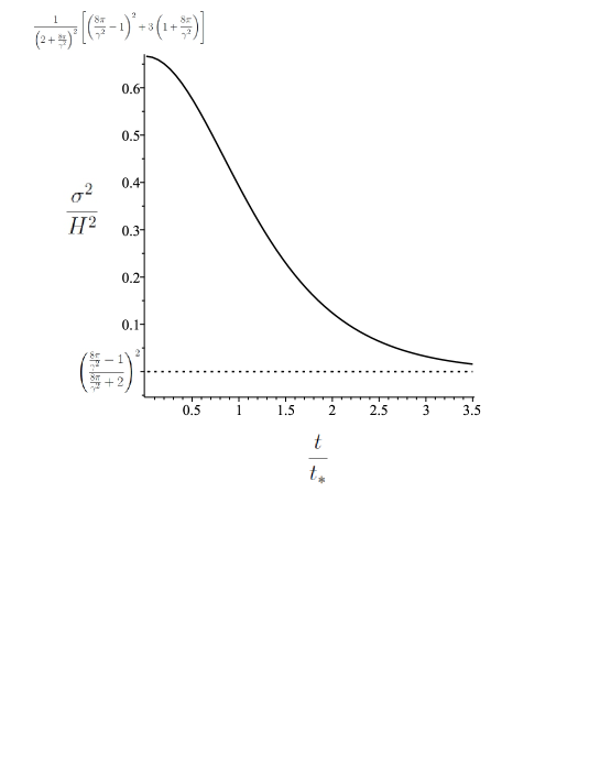
Next, we will consider the anisotropic properties of the model. From (47) and (49) it follows

$$\frac{\sigma^{2}}{H^{2}}=\left(\frac{\frac{8\pi}{\gamma^{2}}-1}{\frac{8\pi}{\gamma^{2}}+2}\right)^{2}+\frac{3}{\left(2+\frac{8\pi}{\gamma^{2}}\right)^{2}}\times$$

$$\times\frac{\sinh^{-\frac{1}{1+\frac{8\pi}{\gamma^{2}}}}\left[t/t_{*}\right]}{\cosh\left[t/t_{*}\right]}\int d\left[t/t_{*}\right]\cdot\sinh^{-\frac{\frac{8\pi}{\gamma^{2}}}{1+\frac{8\pi}{\gamma^{2}}}}\left[t/t_{*}\right]\,,$$ (68)

$$H_{1,2}=\frac{3}{2}H\cdot\frac{1+\frac{8\pi}{\gamma^{2}}}{2+\frac{8\pi}{\gamma^{2}}}\pm\frac{3}{2}H\times$$

$$\times\left\{\left(\frac{\frac{8\pi}{\gamma^{2}}-1}{\frac{8\pi}{\gamma^{2}}+2}\right)^{2}+\frac{4\sinh^{-\frac{1}{1+\frac{8\pi}{\gamma^{2}}}}\left[t/t_{*}\right]}{\left(2+\frac{8\pi}{\gamma^{2}}\right)^{2}\cosh\left[t/t_{*}\right]}\int d\left[t/t_{*}\right]\cdot\sinh^{-\frac{\frac{8\pi}{\gamma^{2}}}{1+\frac{8\pi}{\gamma^{2}}}}\left[t/t_{*}\right]\right\}^{1/2}\,.$$ (69)

Parameter $H_{3}$ remains the same (48).

We mark the necessary properties of the function:

$$\frac{\sinh^{-\frac{1}{1+\frac{8\pi}{\gamma^{2}}}}\left[t/t_{*}\right]}{\cosh\left[t/t_{*}\right]}\int d\left[t/t_{*}\right]\cdot\sinh^{-\frac{\frac{8\pi}{\gamma^{2}}}{1+\frac{8\pi}{\gamma^{2}}}}\left[t/t_{*}\right]\rightarrow 1+\frac{8\pi}{\gamma^{2}},\,\,\text{as}\,\,\,t/t_{*}\rightarrow 0,$$ (70)

$$\frac{\sinh^{-\frac{1}{1+\frac{8\pi}{\gamma^{2}}}}\left[t/t_{*}\right]}{\cosh\left[t/t_{*}\right]}\int d\left[t/t_{*}\right]\cdot\sinh^{-\frac{\frac{8\pi}{\gamma^{2}}}{1+\frac{8\pi}{\gamma^{2}}}}\left[t/t_{*}\right]\propto\exp(-2t/t_{*}),\,\,\text{as}\,\,\,t/t_{*}\rightarrow+\infty.$$ (71)

Figure 2: The profile of the $\sigma^{2}/H^{2}$, $\mu=10^{-4}$.

As seen in Fig. 2, the parameter $\sigma^{2}/H^{2}$ tends monotonically to a constant value over time. It is the bounded function:

$$\left(\frac{\frac{8\pi}{\gamma^{2}}-1}{\frac{8\pi}{\gamma^{2}}+2}\right)^{2}\leq\frac{\sigma^{2}}{H^{2}}\leq\frac{1}{\left(2+\frac{8\pi}{\gamma^{2}}\right)^{2}}\left[\left(\frac{8\pi}{\gamma^{2}}-1\right)^{2}+3\left(1+\frac{8\pi}{\gamma^{2}}\right)\right]\,,\,\,\text{or}$$ (72)

$$\frac{\mu^{2}}{9}\lesssim\frac{\sigma^{2}}{H^{2}}\lesssim\frac{2}{3}\left(1-\frac{\mu}{6}\right)\,.$$ (73)

The anisotropy of the Universe is decreasing, $\sigma^{2}/H^{2}\rightarrow\mu^{2}/9\ll 1$, $t/t_{*}\rightarrow+\infty$.

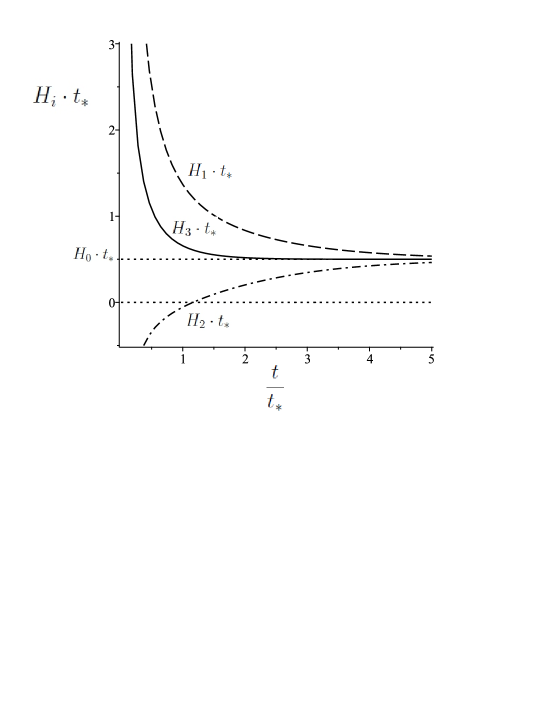
Figure 3: The profile of the $H_{i}\cdot t_{*}$; $H_{0}\cdot t_{*}=\frac{2+\frac{8\pi}{\gamma^{2}}}{3\left(1+\frac{8\pi}{\gamma^{2}}\right)}$, $\mu=10^{-4}$.

As seen in Fig. 3, the functions $H_{i}$ tend monotonically to constant values over time, $t/t_{*}\gg 1$:

$$H_{1}\rightarrow 3H_{0}\cdot\frac{8\pi}{\gamma^{2}\left(2+\frac{8\pi}{\gamma^{2}}\right)};\,\,H_{2},H_{3}\rightarrow 3H_{0}\cdot\frac{1}{2+\frac{8\pi}{\gamma^{2}}}\,,$$ (74)

that is, in this approximation we obtain model (55).

The Universe is expanding along the $x_{1}$ and $x_{3}$ axes: $H_{1,3}>0$. The Hubble parameter $H_{2}$ takes on negative and positive values. The Universe contracts in early times, and expands in late times along axis $x_{2}$. At early time, $t/t_{*}\ll 1$:

$$H_{1,2}\propto\frac{1}{2t}\left\{1\pm\left[1+\frac{4}{\left(2+\frac{8\pi}{\gamma^{2}}\right)^{2}}\right]^{1/2}\right\}\approx\frac{1\pm\sqrt{2}}{2t},\,\,H_{2}<0\,,$$ (75)

$$H_{3}\propto\frac{1}{t\left(1+\frac{8\pi}{\gamma^{2}}\right)}\approx\frac{1}{2t}\,.$$ (76)

At early times scalar factors have the approximation:

$$a_{1,2}\propto\left(\frac{t}{t_{*}}\right)^{\frac{1}{2}\left\{1\pm\left[1+\frac{4}{\left(2+\frac{8\pi}{\gamma^{2}}\right)^{2}}\right]^{1/2}\right\}},\,\,a_{3}\propto\left(\frac{t}{t_{*}}\right)^{\frac{1}{1+\frac{8\pi}{\gamma^{2}}}}\,,\,\,\text{or}$$ (77)

$$a_{1}(a)\sim a^{p_{1}},\,\,a_{2}(a)\sim\frac{1}{a^{|p_{2}|}},\,\,a_{3}(a)=\text{const}\cdot a^{\frac{3}{2+\frac{8\pi}{\gamma^{2}}}}\,,$$ (78)

where

$$p_{1,2}\equiv\frac{3}{2\left(2+\frac{8\pi}{\gamma^{2}}\right)}\left[1+\frac{8\pi}{\gamma^{2}}\pm\left\{\left(\frac{8\pi}{\gamma^{2}}+1\right)^{2}+4\right\}^{1/2}\right]\approx 1\pm\sqrt{2}\,.$$ (79)

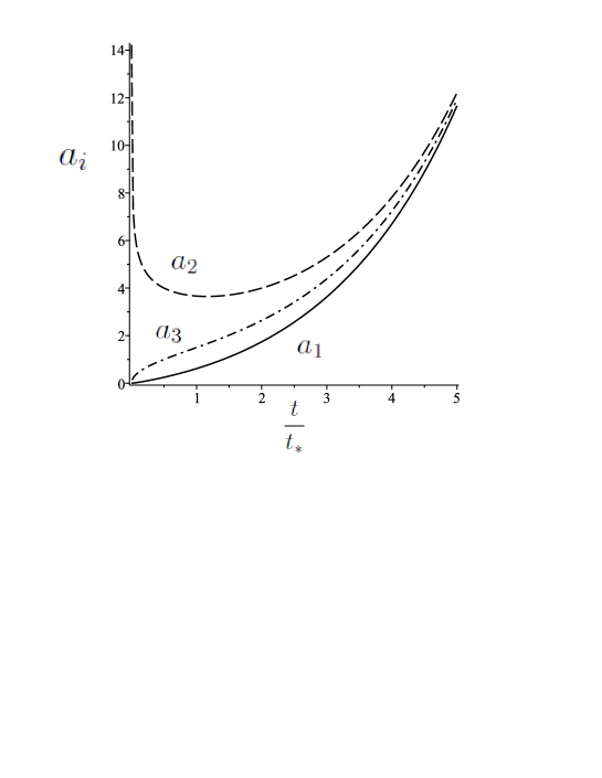
Figure 4: The profile of the $a_{i}(t/t_{*})$ with initial conditions $a_{1}(0.5)=1/4$, $a_{2}(0.5)=4$, $a_{3}(0.5)=1$, $\mu=10^{-4}$.

Scale factors $a_{i}(t)$ are shown in Fig. 4. The figure shows a bouncing scale factor $a_{2}$. The function $a_{2}$ falls from a greater value at the beginning, bounce the minimum value, and then rise again at the end. Other scale factors $a_{1,3}$ start dynamics from zero. At the beginning $t=0$, the Universe is an infinite straight line along axis $x_{2}$: $a_{1}(0)=a_{3}(0)=0$, $a_{2}(0)=+\infty$.

III.3 A massless scalar field

Here we will consider a massless scalar field, $V=0$. In this case from (52) we get

$$\Psi=\Psi_{0}e^{-2\gamma\phi}\,.$$ (80)

Then

$$H^{2}=\frac{8\pi\Psi_{0}c_{0}}{9}\left(2+\frac{8\pi}{\gamma^{2}}\right)\cdot\frac{1}{a^{6}}\,\,\,\text{and}$$ (81)

$$a=\left[8\pi\Psi_{0}c_{0}\left(2+\frac{8\pi}{\gamma^{2}}\right)\right]^{1/6}\cdot t^{1/3}\,,\,\,t\geq 0\,.$$ (82)

Function $\sigma^{2}/H^{2}$ takes the form

$$\frac{\sigma^{2}}{H^{2}}=\left(\frac{\frac{8\pi}{\gamma^{2}}-1}{\frac{8\pi}{\gamma^{2}}+2}\right)^{2}+\frac{3}{\left(2+\frac{8\pi}{\gamma^{2}}\right)^{2}}\cdot\ln\left(\left[8\pi\Psi_{0}c_{0}\left(2+\frac{8\pi}{\gamma^{2}}\right)\right]^{1/2}\cdot t\right)\,.$$ (83)

The anisotropy increases indefinitely as the Universe expands. From this position, this model is not interesting to us.

IV Models with controlled anisotropy

Due to the nonlinearity of the equations (22) and (23), the process УanisotropizationФ  is possible SushkovStar ; Tahara . How to avoid unlimited growth of anisotropy at late times? What should be the potential $V(\phi)$ and the function $\Psi(\phi)$? Let’s explore the different possibilities.

IV.1 A constant anirsotropy model

A possible option is to require a constant level of anisotropy $\sigma/H$=const, using the last degree of freedom. Then from (47) it follows

$$\frac{1}{Ha^{3}}\cdot\int dt\,\frac{e^{2\gamma\phi}\Psi(\phi)}{a^{3}}=\text{const},\,\,\text{or}$$

$$\frac{1}{Ha^{3}}\cdot\int da\,\frac{e^{2\gamma\phi}\Psi(\phi)}{Ha^{4}}=\text{const}\,.$$ (84)

System (51), (52), (53), (84) gives functions $V(\phi)$ and $\Psi(\phi)$:

$$V=Ae^{B\phi},\,\,A>0,\,\,B\neq-2\gamma\left(2+\frac{8\pi}{\gamma^{2}}\right),$$ (85)

$$\Psi=-\frac{2ABc_{1}^{6}}{c_{0}\left[B+2\gamma\left(2+\frac{8\pi}{\gamma^{2}}\right)\right]}\exp\left\{\phi\left[B+2\gamma\left(1+\frac{8\pi}{\gamma^{2}}\right)\right]\right\}\,,$$ (86)

for which the anisotropy is constant. The Hubble parameter and the scale factor are, respectively, given by

$$H^{2}=\frac{32\pi A\left(2+\frac{8\pi}{\gamma^{2}}\right)^{2}}{9\left(B/\gamma+2\left(2+\frac{8\pi}{\gamma^{2}}\right)\right)}\left(\frac{c_{1}}{a}\right)^{-\frac{3B}{\gamma}\cdot\frac{1}{2+\frac{8\pi}{\gamma^{2}}}}\,,$$ (87)

$$a=c_{1}\left[-\frac{B}{\gamma}\,\sqrt{\frac{8\pi A}{B/\gamma+2\left(2+\frac{8\pi}{\gamma^{2}}\right)}}\,\,\cdot t\right]^{-\frac{2\gamma}{3B}\left(2+\frac{8\pi}{\gamma^{2}}\right)}\,.$$ (88)

Equality (17) gives the condition

$$\frac{B/\gamma}{B/\gamma+2\left(2+\frac{8\pi}{\gamma^{2}}\right)}<0$$ (89)

and $H^{2}>0$:

$$\frac{1}{B/\gamma+2\left(2+\frac{8\pi}{\gamma^{2}}\right)}>0.$$ (90)

From the last two inequalities it follows

$$-2\left(2+\frac{8\pi}{\gamma^{2}}\right)<B/\gamma<0.$$ (91)

Magnitude $\sigma^{2}/H^{2}$ takes the form

$$\frac{\sigma^{2}}{H^{2}}=\left(\frac{\frac{8\pi}{\gamma^{2}}-1}{\frac{8\pi}{\gamma^{2}}+2}\right)^{2}-\frac{3B/\gamma}{\left(2+\frac{8\pi}{\gamma^{2}}\right)^{2}\left[B/\gamma+2\left(2+\frac{8\pi}{\gamma^{2}}\right)\right]}\,.$$ (92)

Anisotropy is small, $\sigma/H\ll 1$, if

$$\left|\frac{B}{\gamma}\right|\ll 1,$$ (93)

which is consistent with (91).

Constraints (91) and (93) determine the properties of scale factor (88):

$$a=c_{1}\left[\left|\frac{B}{\gamma}\right|\,\left\{\frac{8\pi A}{\left|B/\gamma+2\left(2+\frac{8\pi}{\gamma^{2}}\right)\right|}\right\}^{1/2}\,\,\cdot t\right]^{\left|\frac{2\gamma}{3B}\left(2+\frac{8\pi}{\gamma^{2}}\right)\right|}\,,$$ (94)

where

$$t\geq 0\,\,\text{and}\,\,\left|\frac{2\gamma}{3B}\left(2+\frac{8\pi}{\gamma^{2}}\right)\right|\gg 1.$$ (95)

Therefore, the Universe is expanding with acceleration. In this model we have power-law inflation. This property is true in all directions:

$$a_{1,2}(a)=\text{const}_{1,2}\cdot a^{k_{1,2}},\,\,a_{3}(a)=\text{const}\cdot a^{\frac{3}{2+\frac{8\pi}{\gamma^{2}}}}\,,$$ (96)

where

$$k_{1,2}=\frac{3}{2}\cdot\frac{1+\frac{8\pi}{\gamma^{2}}}{2+\frac{8\pi}{\gamma^{2}}}\pm$$

$$\pm\sqrt{\frac{9}{4}\left(\frac{\frac{8\pi}{\gamma^{2}}-1}{\frac{8\pi}{\gamma^{2}}+2}\right)^{2}+\frac{9|B/\gamma|}{\left(2+\frac{8\pi}{\gamma^{2}}\right)^{2}\left[B/\gamma+2\left(2+\frac{8\pi}{\gamma^{2}}\right)\right]}}\approx 1,\,\,\frac{3}{2+\frac{8\pi}{\gamma^{2}}}\approx 1.$$ (97)

The Universe begins its evolution from the point: $a_{i}(0)=0.$

IV.2 Model with dynamic anisotropy

Here we will assume

$$\frac{8\pi}{\left(2+\frac{8\pi}{\gamma^{2}}\right)Ha^{3}}\cdot\int da\,\frac{c_{0}e^{2\gamma\phi}\Psi(\phi)}{Ha^{4}}=A^{2}_{0}\left(\frac{c_{1}}{a}\right)^{n},\,\,n>0\,,$$ (98)

then during the Universe expansion the anisotropy will decrease and tend to a small value:

$$\frac{\sigma^{2}}{H^{2}}=\left(\frac{\frac{8\pi}{\gamma^{2}}-1}{\frac{8\pi}{\gamma^{2}}+2}\right)^{2}+A^{2}_{0}\left(\frac{c_{1}}{a}\right)^{n},\,\,\frac{\sigma^{2}}{H^{2}}\rightarrow\left(\frac{\frac{8\pi}{\gamma^{2}}-1}{\frac{8\pi}{\gamma^{2}}+2}\right)^{2}\ll 1,\,\,\text{as}\,\,\,a\rightarrow+\infty.$$ (99)

System (51), (52), (53), (98) gives functions $V(\phi)$ and $\Psi(\phi)$:

$$V=\frac{\Psi_{0}c_{0}}{2c_{1}^{6}(3-n)}\left(ne^{-\gamma\phi n\left(2+\frac{8\pi}{\gamma^{2}}\right)/3}+\frac{9}{A^{2}_{0}\left(2+\frac{8\pi}{\gamma^{2}}\right)^{2}}\right)\times$$

$$\times\left[e^{-\gamma\phi n\left(2+\frac{8\pi}{\gamma^{2}}\right)/3}+\frac{3}{A^{2}_{0}\left(2+\frac{8\pi}{\gamma^{2}}\right)^{2}}\right]^{3(2-n)/n}\,,\,\,0<n<3\,,$$ (100)

$$\Psi=\Psi_{0}e^{\gamma\phi\left[2\left(1+\frac{8\pi}{\gamma^{2}}\right)-n\left(2+\frac{8\pi}{\gamma^{2}}\right)/3\right]}\left[e^{-\gamma\phi n\left(2+\frac{8\pi}{\gamma^{2}}\right)/3}+\frac{3}{A^{2}_{0}\left(2+\frac{8\pi}{\gamma^{2}}\right)^{2}}\right]^{3(2-n)/n}\,.$$ (101)

The Hubble parameters have the form:

$$H^{2}=\frac{8\pi}{3}\left(2+\frac{8\pi}{\gamma^{2}}\right)\frac{\Psi_{0}c_{0}}{c_{1}^{6}(3-n)}\left[\left(\frac{c_{1}}{a}\right)^{n}+\frac{3}{A^{2}_{0}\left(2+\frac{8\pi}{\gamma^{2}}\right)^{2}}\right]^{2(3-n)/n}\,,$$ (102)

$$H_{1,2}=H\left[\frac{3}{2}\cdot\frac{1+\frac{8\pi}{\gamma^{2}}}{2+\frac{8\pi}{\gamma^{2}}}\pm\sqrt{\frac{9}{4}\cdot\left(\frac{\frac{8\pi}{\gamma^{2}}-1}{\frac{8\pi}{\gamma^{2}}+2}\right)^{2}+3A^{2}_{0}\left(\frac{c_{1}}{a}\right)^{n}}\,\,\right]\,.$$ (103)

Parameter $H_{3}$ remains the same (48).

Scale factors $a_{i}$ are expressed through the scale factor $a$:

$$a_{1,2}=s_{1,2}\cdot\left(\frac{a}{c_{1}}\right)^{\frac{3}{2}\cdot\frac{1+\frac{8\pi}{\gamma^{2}}}{2+\frac{8\pi}{\gamma^{2}}}}\left[\sqrt{1+\frac{\nu^{2}}{3A^{2}_{0}}\left(\frac{a}{c_{1}}\right)^{n}}+\sqrt{\frac{\nu^{2}}{3A^{2}_{0}}\left(\frac{a}{c_{1}}\right)^{n}}\,\right]^{\pm\frac{2|\nu|}{n}}\times$$

$$\times\exp\left\{\mp\frac{2}{n}\cdot\sqrt{\nu^{2}+3A^{2}_{0}\left(\frac{c_{1}}{a}\right)^{n}}\,\right\},\,\,\nu^{2}\equiv\dfrac{9}{4}\cdot\left(\dfrac{\frac{8\pi}{\gamma^{2}}-1}{\frac{8\pi}{\gamma^{2}}+2}\right)^{2}\,,$$ (104)

$$a_{3}=s_{3}\cdot\left(\frac{a}{c_{1}}\right)^{\frac{3}{2+\frac{8\pi}{\gamma^{2}}}},\,\,s_{i}=\text{const},\,\,s_{1}s_{2}s_{3}=c_{1}^{3}\,.$$ (105)

Let’s consider the "geometric mean"  behavior of the Universe. For $a/c_{1}\ll 1$ we have the approximation

$$H^{2}\propto a^{-2(3-n)}\Rightarrow a\sim t^{\frac{1}{3-n}},\,\,t\geq 0.$$ (106)

Since $0<n<3$, then the Universe is expanding. In case $2<n<3$, the Universe is expanding with acceleration.

For $A_{0}^{-2/n}a/c_{1}\gg 1$ we have the approximation $H^{2}\approx$ const, which corresponds to de Sitter type expansion, $a=\text{const}\cdot e^{H_{0}t}$. In case $0<n<2$, the phase of the Universe expansion without acceleration is replaced by a phase of accelerated expansion. When $2<n<3$, the power-law inflation is replaced by the exponential inflation over time.

Figure 5: The profile of the $H_{i}/H_{0}$; $n=3/2$, $A^{2}_{0}=10^{-2}$, $\mu=10^{-4}$.

For example, let’s put $n=3/2$, then

$$H^{2}=\frac{16\pi}{9}\left(2+\frac{8\pi}{\gamma^{2}}\right)\frac{\Psi_{0}c_{0}}{c_{1}^{6}}\left[\left(\frac{c_{1}}{a}\right)^{3/2}+\frac{3}{A^{2}_{0}\left(2+\frac{8\pi}{\gamma^{2}}\right)^{2}}\right]^{2}\,.$$ (107)

Therefore,

$$a=c_{1}\left\{3^{-1}A^{2}_{0}\left(2+\frac{8\pi}{\gamma^{2}}\right)^{2}\left[\exp\left(\frac{3}{2}H_{\infty}t\right)-1\right]\right\}^{2/3}\,,$$ (108)

$$H_{\infty}\equiv\frac{4\sqrt{\pi\Psi_{0}c_{0}}}{c_{1}^{3}A^{2}_{0}\left(2+\frac{8\pi}{\gamma^{2}}\right)^{3/2}},\,\,t\geq 0\,.$$

We have the following approximations:

$$a\propto t^{2/3},\,\,\text{as}\,\,\,H_{\infty}t\ll 1;\,\,\,a\propto e^{H_{\infty}t},\,\,\text{as}\,\,\,H_{\infty}t\gg 1.$$ (109)

The first approximation corresponds to the dark matter with the equation of state parameter $w=0$. The second approximation corresponds to the dark energy with $w=-1$. Thus, a model of a unified description of the dark sector is obtained.

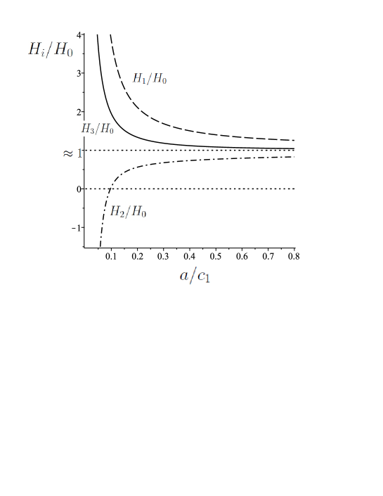
Figure 6: The profile of the $a_{i}/s_{i}$; $n=3/2$, $A^{2}_{0}=10^{-2}$, $\mu=10^{-4}$.

Next, we will consider the anisotropic properties of the model. As seen in Fig. 5, the functions $H_{i}$ tend monotonically to constant values over time, $A_{0}^{-2/n}a/c_{1}\gg 1$:

$$H_{1}\rightarrow 3H_{0}\cdot\frac{8\pi}{\gamma^{2}\left(2+\frac{8\pi}{\gamma^{2}}\right)};\,\,H_{2},H_{3}\rightarrow 3H_{0}\cdot\frac{1}{2+\frac{8\pi}{\gamma^{2}}}\,,$$ (110)

$$H_{0}=\left[\frac{8\pi}{3}\left(2+\frac{8\pi}{\gamma^{2}}\right)\frac{\Psi_{0}c_{0}}{c_{1}^{6}(3-n)}\right]^{1/2}\left[\frac{3}{A^{2}_{0}\left(2+\frac{8\pi}{\gamma^{2}}\right)^{2}}\right]^{(3-n)/n}\,,$$

that is, in this approximation we obtain model (55).

The Universe is expanding along the $x_{1}$ and $x_{3}$ axes: $H_{1,3}>0$. The Hubble parameter $H_{2}$ takes on negative and positive values. The Universe contracts in early times, and expands in late times along axis $x_{2}$. For $A_{0}^{-2/n}a/c_{1}\ll 1$ scalar factors $a_{1,2}$ have the approximation:

$$a_{1,2}(a)\sim\left(\frac{a}{c_{1}}\right)^{\frac{3}{2}\cdot\frac{1+\frac{8\pi}{\gamma^{2}}}{2+\frac{8\pi}{\gamma^{2}}}}\exp\left\{\mp\frac{2\sqrt{3}A_{0}}{n}\cdot\left(\frac{c_{1}}{a}\right)^{n/2}\,\right\}.$$ (111)

Scale factors $a_{i}(a)$ are shown in Fig. 6. The figure shows a bouncing scale factor $a_{2}$. The function $a_{2}$ falls from a greater value at the beginning, bounce the minimum value, and then rise again at the end. Other scale factors $a_{1,3}$ start dynamics from zero. At the beginning $t=0$, the Universe is an infinite straight line along axis $x_{2}$: $a_{1}(0)=a_{3}(0)=0$, $a_{2}(0)=+\infty$.

V Conclusion

We have proposed the reconstruction method in the BI for the subclass of the HG:

$$G_{4}=1/(16\pi),\,\,G_{5}=-\frac{1}{32\pi\gamma X}$$ (112)

with arbitrary functions $G_{2}(X,\phi)$, $G_{3}(X,\phi)$ and with the non-minimal interaction by the law $\Psi(\phi)F_{\mu\nu}F^{\mu\nu}$. Here this method was applied in special case

$$G_{2}=\varepsilon X-V(\phi),\,\,G_{3}=0.$$ (113)

Then the necessary condition for small anisotropy is

$$\varepsilon=1,\,\,\frac{8\pi}{\gamma^{2}}=1+\mu,\,\,|\mu|\ll 1.$$ (114)

This condition is not sufficient.

In the reconstruction framework for theories (113), there is the direct connection (52) between $V(\phi)$ and $\Psi(\phi)$. Using it as first step, we studied cases:

1. Without the magnetic field: $\Psi=0\Rightarrow V=$const. The model has a constant level of anisotropy, $|\sigma/H|=$const$\ll 1$. The Universe has de Sitter type expansion.

2. Minimal coupling with the magnetic field: $\Psi=$const $\Rightarrow\,V=c_{1}+c_{2}\cdot e^{c_{3}\cdot\phi}$, $c_{i}$=const. The anisotropy is limited and decreases to a small value as the Universe expands. In this model, there are two phases of the evolution of the Universe. In the first phase, there is no acceleration, and the second one is characterized by the acceleration expansion of the Universe. There is a anisotropic bounce, $a_{2}$ is a bouncing scale factor. At the beginning $t=0$, the Universe is an infinite straight line along axis $x_{2}$: $a_{1}(0)=a_{3}(0)=0$, $a_{2}(0)=+\infty$.

3. The massless scalar field: $V=0\Rightarrow\,\Psi=\Psi_{0}e^{-2\gamma\phi}$. The anisotropy increases indefinitely as the Universe expands, $\sigma^{2}/H^{2}\propto\ln(t/t_{*})$, $t/t_{*}\rightarrow+\infty$.

We obtained the following models by limiting anisotropy to the first step:

1. The constant level of anisotropy, $1\gg|\sigma/H|$=const $\Rightarrow V=Ae^{B\phi}$ and

   $$\Psi=-\frac{2ABc_{1}^{6}}{c_{0}\left[B+2\gamma\left(2+\frac{8\pi}{\gamma^{2}}\right)\right]}\exp\left\{\phi\left[B+2\gamma\left(1+\frac{8\pi}{\gamma^{2}}\right)\right]\right\}.$$

   In this model we have power-law inflation, $a(t)\sim t^{|\alpha|}$, $|\alpha|\gg 1$.

2. Decreasing anisotropy, $\sigma^{2}/H^{2}=c_{1}+c_{2}/a^{n}$. Then $V$, $\Psi$ have the form (100), (101). In case $0<n<2$, the phase of the Universe expansion without acceleration is replaced by a phase of accelerated expansion. When $2<n<3$, the power-law inflation is replaced by the exponential inflation over time. There is a anisotropic bounce, $a_{2}$ is a bouncing scale factor. At the beginning $t=0$, the Universe is an infinite straight line along axis $x_{2}$: $a_{1}(0)=a_{3}(0)=0$, $a_{2}(0)=+\infty$.

Thus, we solve the question of regulating the anisotropic level. In a more general context, we have found a method of obtaining exact solutions for large subclass of the HG with the electromagnetic field. In the next work, models with $U(a)\neq 0$ (see (39)) are studied.

References

(1) A. G. Doroshkevich, Astrophys. J. 1, 138 (1965)
(2) K. S. Thorne, Astrophys. J. 148, 51 (1967)
(3) K. C. Jacobs, Astrophys. J. 155, 379 (1969)
(4) M. Salimyx, S. L. Sautuyk and R. Martins, Class. Quantum Grav. 15, 1521 (1998)
(5) J. T. Horwood and J. Wainwright, Gen. Rel. Grav. 36, 799 (2004)
(6) K. A. Bronnikov, E. N. Chudayeva and G. N. Shikin, Class. Quantum Grav. 21, 3389 (2004)
(7) M. Watanabe, S. Kanno and J. Soda, PRL 102, 191302 (2009)
(8) J. Soda, Class. Quantum Grav. 29, 083001 (2012)
(9) T.Q. Do, W. F. Kao, Phys. Rev. D 96, 023529 (2017)
(10) D.H. Nguyen, T.M. Pham and T.Q. Do, Eur. Phys. J. C
81, 839 (2021)
(11) G.W. Horndeski: Int. J. Theor. Phys. 10, 363 (1974)
(12) T. Kobayashi, M. Yamaguchi and J. Yokoyama: Prog. Theor. Phys. 126, 511 (2011)
(13) R. K. Muharlyamov, T. N. Pankratyeva, Mod. Phys. Lett. A 34, 1950239 (2019)
(14) H. Amirhashchi and S. Amirhashchi, Phys. Rev. D 99, 023516 (2019)
(15) M. Koussour, H. Filali, S. H. Shekh and M. Bennai, Nuclear Physics B 978, 115738 (2022)
(16) M. Koussour and M. Bennai, Classical and Quantum Gravity 39, 105001 (2022)
(17) O. Akarsu, S. Kumar, S. Sharma and L. Tedesco, Phys. Rev. D 100, 023532 (2019)
(18) P. Sarmah and U. D. Goswami, Mod. Phys. Lett. A 37,
2250134 (2022)
(19) S. W. Hawking and R. J. Taylor, Nature 299,
1278 (1966)
(20) B. L. Hu and L. Parker, Phys. Rev. D 17, 933 (1978)
(21) M. Jamil, D. Momeni, N.S. Serikbayev and R. Myrzakulov, Astrophys Space Sci 339, 37-43 (2012)
(22) M. Jamil, S. Ali, D. Momeni and R. Myrzakulov, Eur. Phys. J. C 72, 1998 (2012)
(23) R. Galeev, R. K. Muharlyamov, A. A. Starobinsky,
S. V. Sushkov and M. S. Volkov, Phys. Rev. D, 103, 104015
(2021)
(24) H. W. H. Tahara, S. Nishi, T. Kobayashi and J. Yokoyama JCAP07, 058 (2018)
(25) W. Rahman et al., Mon. Not. R. Astron. Soc., 514, 139 (2022)
(26) R. K. Muharlyamov, T. N. Pankratyeva, Eur. Phys. J. Plus 136, 590 (2021)
(27) R. K. Muharlyamov, T. N. Pankratyeva, Mod. Phys. Lett. A 37, 2250108 (2022)
(28) R. K. Muharlyamov, T. N. Pankratyeva, Indian J. Phys., 97, 2239Ц2245 (2023)
(29) R. C. Bernardo and J. L. Said: JCAP 09, 014 (2021)
(30) R. C. Bernardo, D. Grandon, J. L. Said and V. H. Cardenas: Phys. Dark Universe
36, 101017 (2022)
(31) K. Bhattacharya and S. Chakraborty, Phys. Rev. D 99, 023520 (2019)
(32) A. De et al., Eur. Phys. J. C, 82, 72 (2022)
(33) A. H. A. Alfedeel and R. K. Tiwari, Indian J. Phys., 96, 1877 (2022)
(34) S. Arora et al. JCAP, 09, 042 (2022)
(35) M. Sharif and A. Majid, Eur. Phys. J. Plus 137, 114 (2022)
(36) F. Esposito, S. Carloni, R. Cianci and S. Vignolo, Phys. Rev. D 105, 084061 (2022)
(37) C. Gao, J. Cosmol. Astropart. Phys. 06 (2010) 023.
(38) L. N. Granda and W. Cardona, J. Cosmol. Astropart. Phys. 07 (2010) 021.
(39) Q. Shafi and C. Wetterich, Phys. Lett. B 152 (1985) 51
(40) Q. Shafi and C. Wetterich, Nucl. Phys. B 289 (1987) 787
(41) S. Hawking and R. Laflamme: Physics Letters B 209, 39 (1988)
(42) L. Campanelli, Phys. Rev. D, 84, 123521