Spread complexity and dynamical transition in two-mode Bose-Einstein condensations
Abstract
We study the spread complexity in two-mode Bose-Einstein condensations and unveil that the long-time average of the spread complexity can probe the dynamical transition from self-trapping to Josephson oscillation. When the parameter increases over a critical value , we reveal that the spread complexity exhibits a sharp transition from lower to higher value, with the corresponding phase space trajectory changing from self-trapping to Josephson oscillation. Moreover, we scrutinize the eigen-spectrum and uncover the relation between the dynamical transition and the excited state quantum phase transition, which is characterized by the emergence of singularity in the density of states at critical energy . In the thermodynamical limit, the cross point of and the initial energy determines the dynamical transition point . Finally, we show that the different dynamical behavior for the initial state at a fixed point can be distinguished by the long-time average of the spread complexity, when the fixed point changes from unstable to stable.
I INTRODUCTION
As a paradigmatic platform for investigating intriguing dynamical phenomena, the two-mode Bose-Einstein condensations (BECs) have attracted intensive studies in past decades (Andrews1997Science, ; Milburn1997PRA, ; Smerzi1997PRL, ; Leggett2001RMP, ; Micheli2003PRA, ; Zhou2003JPAM, ; Mahmud2005PRA, ; LiangCG, ; Tonel2005JPAM, ; Theocharis2006PRE, ). In a two-mode approximation, a two-component BEC or a BEC trapped in a double-well potential can be effectively described by a two-mode or two-site Bose-Hubbard model (Milburn1997PRA, ; Smerzi1997PRL, ; Leggett2001RMP, ; Anglin2001PRA, ; Korsch2007PRA, ; Links2006AHP, ; Folling2007Nature, ; Julia2010PRA, ; Rubeni2017PRA, ; Boukobza2009PRL, ), which is equivalently represented by a large spin model, known as Lipkin-Meshkov-Glick (LMG) model (LMG1965, ; Ma2009PRE, ) in a different parameter region. The two-mode BECs exhibit rich dynamical behaviors, such as Jospheson oscillation (Milburn1997PRA, ; Smerzi1997PRL, ) and self-trapping (Smerzi1999, ; Smerzi2001, ; Albiez2005PRL, ; Liu2006PRA, ), which have been studied in the scheme of nonlinear Schröinger equation and the Bose-Hubbard model. On the other hand, the LMG model is a prototypical model for studying quantum phase transition and excited state phase transition (Corps2021PRL, ; Perez2011PRA, ; Wang2017PRE, ; Santos2016PRA, ; Gamito2022PRE, ; Dusuel2004PRL, ; Relano2009, ). It has been widely applied to study equilibrium and nonequilibrium properties of quantum many-body systems Corps2022PRB ; Corps2023PRL ; Chinni2021PRR ; LMGdyn .
In past years, quenching a quantum system far from equilibrium was used to unveil the exotic dynamical phenomenon, e.g., the long time average of order parameter changes nonanalytically at a dynamical transition point (Sciolla2013PRB, ; Piccitto2019RPB, ; Muniz2020Nature, ; DPT1, ; DPT2, ; DPT3, ), and a series of non-analytical zero points at critical times present in the Loschmidt echo during time evolution (Heyl2013PRL, ; Karrasch2013PRB, ; Jurcevic2017PRL, ; Heyl2019, ; Lang2018, ; Sirker, ; Canovi, ). Both two non-analytical behaviours relate to the intrinsic property of the system and belong to the class of dynamical phase transition. Usually, fully understanding dynamical properties of a many-body system need to be diagnosed by various quantities from different perspectives. The concept of complexity is such a quantity that has been used to characterize the speed of the quantum evolution (Brown2017PRD, ; Balasubramanian2020JHEP, ; Balasubramanian2021JHEP, ). In terms of complexity, the universal properties of operator growth can be seen in the Lanczos coefficients after expanding the operator in Krylov basis (Parker2019PRX, ). Furthermore, the property of a quantum phase also roots in the complexity of a state during the unitary evolution (Sokolov2008PRE, ; Balasubramanian2022PRD, ; Caputa2022PRB, ; Afrasiar2023JSM, ; Caputa2023JHEP, ; Pal2023PRB, ; Pal2023, ) which can be obtained from the quantity named spread complexity. Motivated by these progresses, it is interesting to explore whether complexity can be used as an efficient probe to distinguish different dynamical behaviors in many-body systems.
In this work, we utilize the spread complexity in the Krylov basis to characterize the dynamical transition occurring in two-mode BECs. Usually, this dynamical transition is characterized by the non-analyticity of the long time average of the order parameters in quench dynamics. Here we find that the long-time average of the spread complexity can characterize the dynamical transition in two-mode BECs, consistent with the result obtained from the analysis of dynamical order parameter. It exhibits a transition from the lower complexity to the higher complexity as the phase space trajectory changes from self-trapping to Josephson oscillations. Although the semiclassical phase space dynamics Bohigas1993 provides instructive understanding of the dependence of dynamical transition on the choice of initial state, it is still elusive to understand the role of eigen-spectrum of the underlying Hamiltonian which governs the dynamical evolution. By examining the overlap between the initial state and the eigenstates of the Hamiltonian, we demonstrate that the dynamical behaviour of the quantum system is dominated by small portion of the eigenstates whose energy near the initial state energy. To deepen our understanding, we analyze the structure of spectrum and uncover the relation of dynamical transition with the excited state quantum phase transition EQPT ; EQPT2 , which is characterized by the emergence of singularity in the density of states at critical energy EQPT ; EQPT2 ; Santos2016PRA ; Relano2009 ; Perez2011PRA . Under semiclassical approximation, the critical energy corresponds to the energy of a saddle point, which separates the degenerate region and non-degenerate region. When the parameter increases over a threshold , the saddle point becomes a maximum, and the corresponding dynamics changes dramatically. By studying the dynamics with the initial state at this fixed point, we show that the spread complexity exhibits quite different behavior in the region above or below , and the transition can be characterized by the long-time average of the spread complexity.
The rest of the paper is organized as follows. In section II, we briefly introduce the spread complexity and derive the expression of long-time average of the spread complexity. In section III, we study the dynamical transition in two-mode BECs and demonstrate that the different dynamical behaviors in the self-trapping regime and Josephson oscillation regime can be characterized by the sharp change of the long-time average of spreading complexity. In section IV, we unveil the relation of dynamical transition with the spectrum structure of the underlying Hamiltonian. In section V, we study the dynamical behavior of spreading complexity around a fixed point and demonstrate that different behavior in the region above or below can be characterized by the long-time average of the spread complexity. A summary is given in section VI.
II Long-time average of the spread complexity
Consider a quantum system with a time-independent Hamiltonian . For convenience, we set . Then the time evolution of a state is governed by . Expanding the right hand side in power series, we get
| (1) |
where . Then applying the Gram–Schmidt process to the set of vectors , it generates an orthogonal basis with . The basis is called Krylov basis (Balasubramanian2022PRD, ; Afrasiar2023JSM, ). In this paper, we consider the complete orthonormal basis of the Hillbert space with the maximal value of being , where is the dimension of the Hamiltonian . The full algorithm is described as following: After choosing the initial state , the subsequent Krylov bases can be obtained recursively by following algorithm:
| (2) | ||||
Then the Hamiltonian becomes a tridiagonal form in the Krylov basis :
| (3) |
where and are also called Lanczos coefficients (Viswanath1950, ). In our numerical calculation, we use the MPLAPACK (Nakata2021arXiv, ) library to perform the arbitrary precision computation.
Using the Krylov basis, we can define the spread complexity as (Balasubramanian2022PRD, )
| (4) |
The spread complexity quantifies the degree of complex of the initial state during the time evolution. It can be observed that the return probability is defined as . The return probability is also known as Loschmidt echo and has been widely studied in the non-equilibrium system (Heyl2013PRL, ; Karrasch2013PRB, ; Heyl2019, ; Zhou2019PRB, ; ZengYM, ; ZhouBZ, ). In this paper, we focus on the long time average of the spread complexity
| (5) |
Inserting the complete set of energy eigenstates, we get
| (6) |
where the coefficients are given by with .
III Dynamical transition in two-mode Bose-Einstein condensates
Now, we consider a two-mode Bose-Einstein condensates with the Hamiltonian described by (Leggett2001RMP, ; Micheli2003PRA, ; Tonel2005JPAMG, ; Zibold2010PRL, ; Fan2012PRA, ):
| (7) |
where is atom-atom interaction and is the Rabi frequency of the external field interacting with the condensate. For the sake of convenience, we set as the unit of energy. The angular-momentum operators , and are the Schwinger pseudospin operators:
| (8) |
where and is bosonic creation and annihilation operator, respectively. This many-particle Hamiltonian is closely related to the original LMG model (LMG1965, ), for which however the parameter is negative.
Under the semi-classical approximation with , angular-momentum operators can be replaced by Then we can obtain the equations of motion via the Heisenberg equations of motion:
| (9) | ||||
| (10) |
The classical dynamics has been studied in the previous works which showed the dynamical transition between self-trapped trajectory and Josephson oscillation trajectory. Here, we demonstrate the classical trajectories in Figs. 1(a1)(a4), in which we consider three initial values with and . The four figures corresponding to four different and their trajectories form closed orbits. It can be found that three trajectories show the self-trapped behaviour for small . As increases, the trajectories for different initial state sequentially become Josephson oscillation. Such as in Figs. 1(a2) for , only the trajectory with transition to the Josephson oscillation and others remain self-trapped behaviour. However, in Figs. 1(a3) for , only the trajectory with remains in the self-trapped regime. The dynamical transition of the classical trajectory can be captured by the order parameter which is the time average of the canonical coordinate . In Fig. 1(c), we demonstrate the value of with respect to for three different initial values. Here we carry out the time average from 0 to 1000. It can be found that has a non-zero value for self-trapped trajectories but approaches zero for Josephson oscillation trajectories.

For quantum dynamics, we choose the coherent spin states (CSS) as the initial state (Micheli2003PRA, ; Zhang2021PRB, ). These states are given by
| (11) |
where is the highest-weight state of SU(2) group with spin and . The CSS takes its maximum polarization in the direction . Such a choice of the initial state is relevant to analyze the classical-quantum correspondence. For quantum trajectory, we calculate the time evolved state with and corresponding time dependent expectation value , and . Then we transform into sphere coordinate where . Similar to the classical trajectory, we present the quantum trajectories in the plane, as shown in Figs. 1(b1)(b4). The parameters are the same as in Figs. 1(a1)(a4). It can be observed that the areas of the quantum trajectories are related to the classical trajectories. Particularly, the initial state dependent dynamics transition can also be observed in the quantum trajectory. Similar to the order parameter , we can choose the order parameter in quantum dynamics. In Fig. 1(c), we show the values of by dashed lines and they are similar to the semi-classical ones except that the transition points are smoothen by the finite size effect.


The different distribution of the quantum trajectories can be characterized by the long time average of the spread complexity which is displayed in Fig. 1(d). It can be found that the larger accessible area of trajectory corresponds to the larger value of the spread complexity and vice verse. The connection between quantum trajectories and the spread complexity is intuitive. For the self-trapped trajectories, the time-evolved state is constrained in a small area of the phase space. In the perspective of Krylov space, the self-trapped trajectory is dynamically localized near the space of the initial Krylov state . For the extremely localized case, the dynamics is frozen at initial state and we have and . However, for the Josephson oscillation trajectories, the time-evolved state extends in the phase space and widely distributes in the Krylov space. Considering the maximally delocalized state in Krylov space, we have and . The value is drawn by the red-bolded line for in Fig. 1(d). It can be seen that is closer to the value for the larger area of quantum trajectory.
Next we carry out the finite size analyse on the transition point. To determine the transition point, we differentiate the function with respect to and label the location of the maximum of as , which is size dependent. We show for different size in Fig.2(c) and Fig.2 (d). Further linear fitting the results of indicate the transition point at large limit is for and for . These converged values are close to the transition point and present in the order parameter in Fig. 1(c).
IV Relation to the spectrum structure
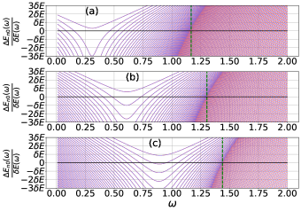
To unveil the relation of dynamical transition to the spectrum structure, we examine the eigen-spectrum of two-mode BEC with respect of . Here, we sort the eigenvalues in such a way that and divide the set into two subsets and . In Fig. (3)(a), we display the values of and , corresponding to the blue dashed lines and red solid lines, respectively. Further considering the initial energy , it can be found the initial energies corresponding to three initial states discussed previously go from the doubly degenerate regime to the non-degenerate regime as increases. The critical energy separates the doubly degenerate regime from the non-degenerate regime in the thermodynamic limit. As depicted in Figs. 3(b)(c)(d), the critical energy can be evidenced by the local divergence in the density of states (Santos2016PRA, ). While states below are non-degenerate, the states above are degenerate in the thermodynamic limit. For a finite size system, it should be noted that the gap of the doubly degenerate energy is exponentially small. With the increasing of , the region of doubly degenerate shrinks and eventually vanishes at . The critical energy for is equal to the initial energy with the initial state , marked by the black dashed line in Fig. (3)(a). For a quantum system, and as for . Meanwhile, under the semi-classical approximation, we can obtain , consistent with the result of the quantum system in the thermodynamic limit.
Now we introduce the energy uncertainty of the initial state , which is calculated by
| (12) |
Then we construct the Gaussian function from and :
| (13) |
where is normalized coefficient. The quantity gives the information of how the initial state distributes within eigenstates of the underlying Hamiltonian . We plot the function and the coefficients versus in Fig. 4. It can be found that almost recovers the distribution of , indicating that the distribution of is similar to the Gaussian function with the center located at . Also, we calculate the Eq. (6) within the energy window and present the results in Fig. 1(d) by dashed lines. The results fit very well with the original data and capture the behaviour of the transition. The normal distribution structure of the probability density function means the behaviour of is dominated by a small portion of eigenstates with eigenvalues near the initial energy. Focusing on the part of spectrum near the initial energy , we consider the shifted spectrum with the unit of and display it in Figs. 5. It can be observed that the structure of energy spectrum changes from two-fold degenerate region to non-degenerate region within the energy window as increases. The transition point indicated by the dashed line is around the cross point of and . Since is dependent on the initial state, its cross point with depends on the initial state too (see Fig.3 (a)). This gives an explanation why the dynamical phase transition point is initial-state-dependent from the perspective of spectrum structure.

Similar to the case of LMG model, a symmetry-breaking transition of eigenstates in the two-mode BECs can be triggered by the excited state quantum phase transitions. For the doubly degenerate eigenstate , we can adopt the notion of the partial symmetry introduced in the study of the excited state quantum phase transition (Corps2022PRB, ; Corps2023PRL, ), with the partial symmetry operator defined as . The partial symmetry operator is a operator, which fulfills .
The time evolved state can be expanded in the eigenstates of the Hamiltonian:
| (14) |
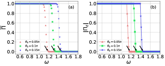
Since our initial state satisfies , when , the time evolved state is restricted in the one of two symmetry subspaces, and thus is conserved. On the contrary, as the parameter cross the transition point, is not conserved. To see it clearly, we numerically calculate the long-time average of the operator :
and the average value of within the energy window , which can be expressed as
| (15) |
where is the number of eigenstates in the energy window . The values of and with respect to are shown in Fig. 6. The transition behaviour presented in and is consistent with the results of Fig.1(c) and Fig.1(d). For , both and equal to 1 as populates within the broken symmetry state. On the other hand, they approach zero for .
V Dynamical behaviour of around a fixed point
Now we study the dynamics around the fixed point . In the regime of , is a saddle point from the perspective of energy surface, denoted by the square symbol in Fig. 7 (a). Besides, there are two degenerate maximums: and , denoted by the star symbol and the triangular symbol in Fig. 7 (a) for , respectively. These two maximums merge into one point at . For , there is only a maximum at , as demonstrated in Fig. 7 (b) for . When increases over the threshold , the trajectory is also dramatically changed, and the corresponding dynamics changes from the Josephson oscillation to the Rabi oscillation (Leggett2001RMP, ; Zibold2010PRL, ). This transition can be characterized by the fixed point whose the Jacobian matrix is
| (16) |
The two eigenvalues of the matrix are . For , two eigenvalues are real number and mutually opposite. So this fixed point is the unstable saddle point. As shown in Fig. 7(a) for , the tangent vector is away from the fixed point. For , two eigenvalues are imaginary number. So the fixed point is stable and called center(Strogatz2014, ) whose nearby trajectories are neither attracted to nor repelled from the fixed point, as illustrated in Fig. 7(b). The threshold point splits two qualitatively different dynamical behavior, i.e., Josephson-type versus Rabi-type oscillation.
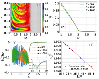
For the quantum system, it has been revealed the existence of exotic dynamical behavior around unstable fixed points (Cao2020PRL, ; Hummel2019PRL, ; Richter2023, ; Kidd2021, ; Bhattacharjee2022JHEP, ), which is refereed to the scrambling characterized by the exponential growth of the out-of-time order correlators. Setting the initial state as , we study how the spread complexity changes with . Here, we show the value of the spread complexity and its long-time average value in Fig. 8(a) and Fig. 8(b), respectively. The dynamics of the suggests that the initial state would evolve to states far away from for , but stays near the initial state for . The dramatically distinct behaviour presented in the is also evidenced by the long time average . When , approaches to zero, as shown in Fig. 8(b).

From the view of the shifted spectrum (Figs. 8(d)) and the overlap (Figs. 8(e)(f)), it can be observed that is highly concentrated on the highest eigenstate for . For the limit case with , the Hamiltonian can be simplified as , and the initial state is the eigenstate of . After dropping a global phase, is time independent in the large limit and the spread complexity maintains zero during the time evolution. For , the initial energy ( for the initial state equals to the critical energy which separates the self-trapped trajectory and Josephson-type trajectory. The distribution of suggests that eigenstates in both the doubly degenerate and non-degenerate regions contribute to , which takes a nonzero value. Additional, the derivative of the with respect to displays oscillation for . The oscillation origin from the quantum fluctuation near the critical energy as the density of state exhibits local divergence.

For the trajectory starting from the fixed point , the dynamics of a classical state is frozen on the plane. However, the remaining radial coordinate of a quantum trajectory is not conserved during the time evolution. Then, we can define the distance of the time evolved state away from the initial state in the phase space as
| (17) |
It can be expected that the distance connects to the state complexity because they both measure the distance between time evolved state and the initial state. To see it clearly, we display the short-time dynamics of with respect to the parameter in the Fig. 9(a) and its long-time average value in Fig. 9(b). Comparing Figs. 8(a)(b) and Fig. 9(a)(b), it can be seen that the dynamical behaviour of is very similar to the dynamical behaviour of . The derivative of the with respect to also shows oscillation for . The similarity between and results from that both of them quantify the distance between time evolved state and the initial state. Here, we can label the location of the minimum of near as an effective transition point , which is guided by the black dashed lines in the insert of Fig. 9(c). It can be seen that separates the oscillation and non-oscillation regime of . From the result of finite size scaling shown in Fig. 9(d), we can obtain , which is approximately equal to the threshold point . The transition point in is the same as because they share the same physical origin.
VI Summary
In summary, we have studied the spread complexity and its long-time average value in the two-mode BECs. Our results demonstrate that the long-time average of the spread complexity can probe the dynamical transition in the two-mode BECs. By choosing spin coherent state as the initial state, we find that exhibits a sharp transition as the phase space trajectory of the time evolved state changes from the self-trapping to Josephson oscillation. By examining the eigen-spectrum of the underlying Hamiltonian, we identified the existence of an excited state quantum phase transition in the region of , characterized by the emergence of singularity in the density of states at critical energy . In the thermodynamical limit, the critical energy separates doubly degenerate eigenstates from non-degenerate eigenstates. We unraveled that the dynamical transition point is determined by the cross point of the initial energy and . When exceeds a threshold , the fixed point changes from a saddle point to a stable fixed point. By studying the dynamics for the initial state at this fixed point, we unveiled that the different dynamical behavior in the region of and can be distinguished by the long-time average of the spread complexity.
Acknowledgements.
This work is supported by National Key Research and Development Program of China (Grant No. 2021YFA1402104 and 2023YFA1406704), the NSFC under Grants No. 12174436 and No. T2121001, and the Strategic Priority Research Program of Chinese Academy of Sciences under Grant No. XDB33000000.References
- (1) M. R. Andrews, C. G. Townsend, H.-J. Miesner, D. S. Durfee, D. M. Kurn, W. Ketterle, Observation of Interference Between Two Bose Condensates, Science 275, 31 (1997).
- (2) G. J. Milburn, J. Corney, E. M. Wright, and D. F. Walls, Quantum dynamics of an atomic Bose-Einstein condensate in a double-well potential, Phys. Rev. A 55, 4318 (1997).
- (3) A. Smerzi, S. Fantoni, S. Giovanazzi, and S. R. Shenoy, Quantum Coherent Atomic Tunneling between Two Trapped Bose-Einstein Condensates, Phys. Rev. Lett. 79, 4950 (1997).
- (4) A. J. Leggett, Bose-Einstein condensation in the alkali gases: Some fundamental concepts, Rev. Mod. Phys. 73, 307 (2001).
- (5) A. Micheli, D. Jaksch, J. I. Cirac, and P. Zoller, Many-particle entanglement in two-component Bose-Einstein condensates, Phys. Rev. A 67, 013607 (2003).
- (6) H.-Q. Zhou, J. Links, R. H McKenzie1 and X.-W. Guan , Exact results for a tunnel-coupled pair of trapped Bose–Einstein condensates, J. Phys. A: Math. Gen. 36, L113 (2003).
- (7) K. W. Mahmud, H. Perry, and W. P. Reinhardt, Quantum phase-space picture of Bose-Einstein condensates in a double well, Phys. Rev. A 71, 023615 (2005).
- (8) A. P. Tonel, J. Links and A. Foerster, Quantum dynamics of a model for two Josephson-coupled Bose–Einstein condensates, J. Phys. A: Math. Gen. 38, 1235 (2005).
- (9) G. Theocharis, P. G. Kevrekidis, D. J. Frantzeskakis,1 and P. Schmelcher, Symmetry breaking in symmetric and asymmetric double-well potentials, Phys. Rev. E 74, 056608 (2006).
- (10) C. Liang, Y. Zhang and S. Chen, Statistical and dynamical aspects of quantum chaos in a kicked Bose-Hubbard dimers, arXiv:2312.08159, Phys. Rev. A 109, xxxxx (2024).
- (11) J. R. Anglin, P. Drummond and A. Smerzi, Exact quantum phase model for mesoscopic Josephson junctions, Phys. Rev. A 64, 063605 (2001).
- (12) E. M. Graefe and H. J. Korsch, Semiclassical quantization of an N-particle Bose-Hubbard model, Phys. Rev. A 76, 032116 (2007).
- (13) S. Fölling, S. Trotzky, P. Cheinet, M. Feld, R. Saers, A. Widera1, T. Müller1 and I. Bloch, Direct observation of second-order atom tunnelling, Nature 448, 1029 (2007).
- (14) J. Links, A. Foerster, A. P. Tonel & G. Santos, The Two-Site Bose–Hubbard Model, Ann. Henri Poincaré 7, 1591 (2006).
- (15) B. Juliá-Díaz, D. Dagnino, M. Lewenstein, J. Martorell, and A. Polls, Macroscopic self-trapping in Bose-Einstein condensates: Analysis of a dynamical quantum phase transition, Phys. Rev. A 81, 023615 (2010).
- (16) D. Rubeni, J. Links and P. S. Isaac, Two-site Bose-Hubbard model with nonlinear tunneling: Classical and quantum analysis, Phys. Rev. A 95, 043607 (2017).
- (17) E. Boukobza, M. Chuchem,D. Cohen and A. Vardi, Phase-Diffusion Dynamics in Weakly Coupled Bose-Einstein Condensates, Phys. Rev. Lett. 102, 180403 (2009).
- (18) H. J. Lipkin, N. Meshkov, and A. J. Glick, Validity of many-body approximation methods for a solvable model: (I). Exact solutions and perturbation theory, Nucl. Phys. 62, 188 (1965).
- (19) J. Ma, X. Wang, and S. Gu, Many-body reduced fidelity susceptibility in Lipkin-Meshkov-Glick mode, Phys. Rev. E 80, 021124 (2009).
- (20) S. Raghavan, A. Smerzi, S. Fantoni, and S. R. Shenoy, Coherent oscillations between two weakly coupled Bose-Einstein condensates: Josephson effects, oscillations, and macroscopic quantum self-trapping, Phys. Rev. A 59, 620 (1999).
- (21) J. R. Anglin, P. Drummond, and A. Smerzi, Exact quantum phase model for mesoscopic Josephson junctions, Phys. Rev. A 64, 063605 (2001).
- (22) M. Albiez, R. Gati, J. Föllling, S. Hunsmann, M. Cristiani, and M. K. Oberthaler, Direct Observation of Tunneling and Nonlinear Self-Trapping in a Single Bosonic Josephson Junction, Phys. Rev. Lett. 95, 010402 (2005).
- (23) G.-F. Wang, L.-B. Fu, and J. Liu, Periodic modulation effect on self-trapping of two weakly coupled Bose-Einstein condensates, Phys. Rev. A 73, 013619 (2006).
- (24) S. Dusuel and J. Vidal, Finite-Size Scaling Exponents of the Lipkin-Meshkov-Glick Model, Phys. Rev. Lett. 93, 237204 (2004).
- (25) P. Pérez-Fernández, A. Relano, J. M. Arias, J. Dukelsky, and J. E. Garcia-Ramos, Decoherence due to an excited-state quantum phase transition in a two-level boson model, Phys. Rev. A 80, 032111 (2009).
- (26) P. Pérez-Fernández, P. Cejnar, J. M. Arias, J. Dukelsky, J. E. García-Ramos, and A. Relaño, Quantum quench influenced by an excited-state phase transition, Phys. Rev. A 83, 033802 (2011).
- (27) L. F. Santos, M. Távora and F. Pérez-Bernal, Excited-state quantum phase transitions in many-body systems with infinite-range interaction: Localization, dynamics, and bifurcation, Phys. Rev. A 94, 012113 (2016).
- (28) Á. L. Corps and A. Relaño, Constant of Motion Identifying Excited-State Quantum Phases, Phys. Rev. Lett. 127, 130602 (2021).
- (29) J. Gamito, J. Khalouf-Rivera, J. M. Arias, P. Pérez-Fernéndez,and F. Pérez-Bernal, Excited-state quantum phase transitions in the anharmonic Lipkin-Meshkov-Glick model: Static aspects, Phys Rev E 106, 044125 (2022).
- (30) Q. Wang and H. T. Quan, Probing the excited-state quantum phase transition through statistics of Loschmidt echo and quantum work, Phys. Rev. E 96, 032142 (2017).
- (31) Á. L. Corps and A. Relaño, Dynamical and excited-state quantum phase transitions in collective systems, Phys. Rev. B 106, 024311 (2022).
- (32) Á. L. Corps and A. Relaño, Theory of Dynamical Phase Transitions in Quantum Systems with Symmetry-Breaking Eigenstates, Phys. Rev. Lett. 130, 100402 (2023).
- (33) K. Chinni, P. M. Poggi, and I. H. Deutsch, Effect of chaos on the simulation of quantum critical phenomena in analog quantum simulators, Phys. Rev. Res. 3, 033145 (2021).
- (34) Angelo Russomanno, Fernando Iemini, Marcello Dalmonte, and Rosario Fazio, Floquet time crystal in the Lipkin-Meshkov-Glick model, Phys. Rev. B 95, 214307 (2017).
- (35) M. Eckstein and M. Kollar, Nonthermal Steady States after an Interaction Quench in the Falicov-Kimball Model, Phys. Rev. Lett. 100, 120404 (2008).
- (36) M. Moeckel and S. Kehrein, Interaction Quench in the Hubbard Model, Phys. Rev. Lett. 100, 175702 (2008).
- (37) B. Sciolla and G. Biroli, Quantum Quenches and Off-Equilibrium Dynamical Transition in the Infinite-Dimensional Bose-Hubbard Model, Phys. Rev. Lett. 105, 220401 (2010).
- (38) B. Sciolla and G. Biroli, Quantum quenches, dynamical transitions, and off-equilibrium quantum criticality, Phys. Rev. B 88, 201110(R) (2013).
- (39) G. Piccitto, B. Žunkovič, and A. Silva, Dynamical phase diagram of a quantum Ising chain with long-range interactions, Phys. Rev. B 100, 180402(R) (2019).
- (40) J. A. Muniz,D. Barberena, R. J. Lewis-Swan1, D. J. Young, J. R. K. Cline1, A. M. Rey and J. K. Thompson, Exploring dynamical phase transitions with cold atoms in an optical cavity, Nature 580, 602 (2020).
- (41) M. Heyl, A. Polkovnikov, and S. Kehrein, Dynamical quantum phase transitions in the transversefield Ising model, Phys. Rev. lett. 110, 135704 (2013).
- (42) C. Karrasch and D. Schuricht, Dynamical phase transitions after quenches in nonintegrable models, Phys. Rev. B 87, 195104 (2013).
- (43) M. Heyl, Dynamical quantum phase transitions: A survey, Europhys. Lett. 125, 26001 (2019).
- (44) E. Canovi, P. Werner, and M. Eckstein, First-Order Dynamical Phase Transitions, Phys. Rev. Lett. 113, 265702 (2014).
- (45) F. Andraschko and J. Sirker, Dynamical quantum phase transitions and the Loschmidt echo: A transfer matrix approach, Phys. Rev. B 89, 125120 (2014).
- (46) J. Lang, B. Frank, and J. C. Halimeh, Dynamical Quantum Phase Transitions: A Geometric Picture, Phys. Rev. Lett. 121, 130603 (2018).
- (47) P. Jurcevic, H. Shen, P. Hauke, C. Maier, T. Brydges, C. Hempel, B. P. Lanyon, M. Heyl, R. Blatt, and C. F. Roos, Direct Observation of Dynamical Quantum Phase Transitions in an Interacting Many-Body System, Phys. Rev. Lett. 119, 080501 (2017).
- (48) A.R. Brown, L. Susskind, and Y. Zhao, Quantum complexity and negative curvature, Phys. Rev. D 95, 045010 (2017).
- (49) V. Balasubramanian, M. DeCross, A. Kara and O. Parrikar, Quantum complexity of time evolution with chaotic Hamiltonians, JHEP 01, 134 (2020).
- (50) V. Balasubramanian, M. DeCross, A. Kar, Y. C. Li and O. Parrikar, Complexity growth in integrable and chaotic models, JHEP 07, 011 (2021).
- (51) D. E. Parker, X. Cao, A. Avdoshkin, T. Scaffidi, and E. Altman, A Universal Operator Growth Hypothesis, Phys. Rev. X 9, 041017 (2019).
- (52) V. V. Sokolov, O. V. Zhirov, G. Benenti, and G. Casa, Complexity of quantum states and reversibility of quantum motion, Phys. Rev. E 78, 046212 (2008).
- (53) V. Balasubramanian , P. Caputa, J. M. Magan, and Q. Wu, Quantum chaos and the complexity of spread of states, Phys. Rev. D 106, 046007 (2022).
- (54) P. Caputa and S. Liu, Quantum complexity and topological phases of matter, Phys. Rev. B 106, 195125 (2022).
- (55) K. Pal, K. Pal, A. Gill, and T. Sarkar, Time evolution of spread complexity and statistics of work done in quantum quenches, Phys. Rev. B 108, 104311 (2023).
- (56) M. Afrasiar, J. K. Basak, B. Dey, K. Pal and K. Pal, Time evolution of spread complexity in quenched Lipkin–Meshkov–Glick model, J. Stat. Mech. 2023, 103101 (2023).
- (57) K. Pal, K. Pal, and T. Sarkar, Complexity in the Lipkin-Meshkov-Glick model, Phys. Rev. E 107, 044130 (2023).
- (58) P Caputa, N. Gupta, S. S. Haque, S. Liu, J. Muruganb and H. J.R. V. Zyl, Spread Complexity and Topological Transitions in the Kitaev Chain, JHEP 01, 120 (2023).
- (59) O. Bohigas, S. Tomsovic, and D. Ullmo, Manifestations of Classical Phase Space Structures in Quantum Mechanics, Phys. Rep. 223, 43 (1993).
- (60) P. Cejnar, M. Macek, S. Heinze, J. Jolie, and J. Dobes, Monodromy and excited-state quantum phase transitions in integrable systems: collective vibrations of nuclei, J. Phys. A: Math. Gen. 39, L515 (2006).
- (61) M. A. Caprio, P. Cejnar, and F. Iachello, Excited-state quantum phase transitions in many-body systems, Ann. Phys. (Amsterdam) 323, 1106 (2008).
- (62) V. Viswanath and G. Müller, The Recursion Method: Application to Many-Body Dynamics (Springer Science Business Media, Berlin, 1994), Vol. 23.
- (63) M. Nakata, MPLAPACK version 2.0.1 user manual, arxiv:2109.13406.
- (64) B. Zhou, C. Yang and S. Chen, Signature of a nonequilibrium quantum phase transition in the long-time average of the Loschmidt echo, Phys. Rev. B 100, 184313 (2019).
- (65) B. Zhou, Y. Zeng, and S. Chen, Exact zeros of the Loschmidt echo and quantum speed limit time for the dynamical quantum phase transition in finite-size systems, Phys. Rev. B 104, 094311 (2021).
- (66) Y. Zeng, B. Zhou, and S. Chen, Dynamical singularity of the rate function for quench dynamics in finite-size quantum systems, Phys. Rev. B 107, 134302 (2023).
- (67) A. P. Tonel, J. Links and A. Foerster, Quantum dynamics of a model for two Josephson-coupled Bose–Einstein condensates, J. Phys. A: Math. Gen. 38, 1235 (2005).
- (68) T. Zibold, E. Nicklas, C. Gross, and M. K. Oberthaler, Classical Bifurcation at the Transition from Rabi to Josephson Dynamics, Phys. Rev. Lett. 105, 204101 (2010).
- (69) W. Fan, Y. Xu, B. Chen, Z. Chen, X. Feng, and C. H. Oh, Quantum phase transition of two-mode Bose-Einstein condensates with an entanglement order parameter, Phys. Rev. A 85, 013645 (2012).
- (70) H. Zhang, and C. D. Batista, Classical spin dynamics based on SU() coherent states, Phys. Rev. B 104, 104409 (2021).
- (71) S. H. Strogatz, Nonlinear Dynamics and Chaos (CRC Press, Boca Raton, 2018).
- (72) T. Xu, T. Scaffidi, and X. Cao, Does Scrambling Equal Chaos, Phys. Rev. Lett. 124, 140602 (2020).
- (73) Q. Hummel, B. Geiger, J. D. Urbina, and K. Richter, Reversible Quantum Information Spreading in Many-Body Systems near Criticality, Phys. Rev. Lett. 123, 160401 (2019).
- (74) R. A. Kidd, A. Safavi-Naini, and J. F. Corney, Saddle-point scrambling without thermalization, Phys. Rev. A 103, 033304 (2021).
- (75) M. Steinhuber, P. Schlagheck, J. D. Urbina, and K. Richter, Dynamical transition from localized to uniform scrambling in locally hyperbolic systems, Phys. Rev. E 108, 024216 (2023).
- (76) B. Bhattacharjee, X. Cao, P. Nandy and T. Pathak, Krylov complexity in saddle-dominated scrambling, JHEP. 05, 174 (2022).