ALPINE: a climbing robot for operations in mountain environments

Abstract

Mountain slopes are perfect examples of harsh environments in which humans are required to perform difficult and dangerous operations such as removing unstable boulders, dangerous vegetation or deploying safety nets. A good replacement for human intervention can be offered by climbing robots. The different solutions existing in the literature are not up to the task for the difficulty of the requirements (navigation, heavy payloads, flexibility in the execution of the tasks). In this paper, we propose a robotic platform that can fill this gap. Our solution is based on a robot that hangs on ropes, and uses a retractable leg to jump away from the mountain walls. Our package of mechanical solutions, along with the algorithms developed for motion planning and control, delivers swift navigation on irregular and steep slopes, the possibility to overcome or travel around significant natural barriers, and the ability to carry heavy payloads and execute complex tasks. In the paper, we give a full account of our main design and algorithmic choices and show the feasibility of the solution through a large number of physically simulated scenarios.

[1]organization=Dipartimento di Ingegneria and Scienza dell’Informazione (DISI), University of Trento, addressline=via Sommarive 9, postcode=38123, city=Trento, country=Italy [2]organization=Dipartimento di Ingegneria Industriale (DII), University of Trento, addressline=via Sommarive 9, postcode=38123, city=Trento, country=Italy [3]organization=Dipartimento di Ingegneria Industriale (DII), University of Trento, addressline=via Sommarive 9, postcode=38123, city=Trento, country=Italy [4]organization=Faculty of Engineering, Free University of Bozen-Bolzano, addressline=via Volta 13/A, postcode=39100, city=Bolzano-Bozen, country=Italy [5]organization=Faculty of Engineering, Free University of Bozen-Bolzano, addressline=via Volta 13/A, postcode=39100, city=Bolzano-Bozen, country=Italy [6]organization=Dipartimento di Ingegneria and Scienza dell’Informazione (DISI), University of Trento, addressline=via Sommarive 9, postcode=38123, city=Trento, country=Italy

1 Introduction

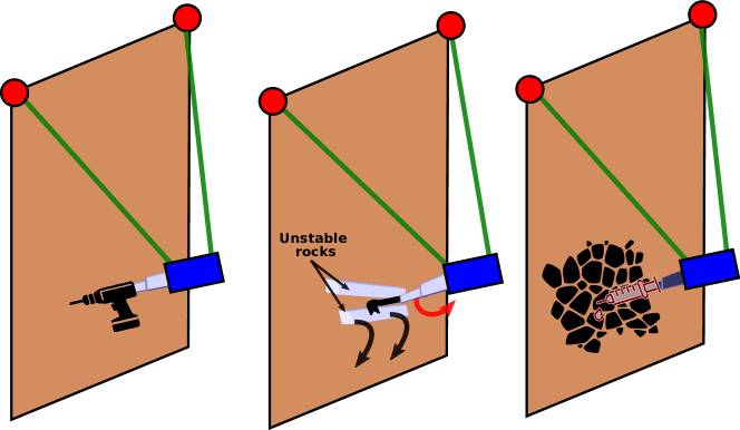
Mountain environments are extremely vulnerable to climate change and often subject to landslides, floods and avalanches. Such ruinous events endanger a large number of economic activities (first and foremost tourism and agriculture) and put at risk the very survival of small towns and villages. Any realistic strategy to counter these risks is necessarily based on constant monitoring and on regular maintenance operations on the mountains slopes. Such activities include detaching from the mountain walls dangerous boulders (a.k.a. scaling), loosing potentially unstable shrubs and bushes, and deploying landslide protection networks. The interested areas are often difficult to reach and maintenance activities are typically performed manually by highly trained human operators. These tasks are challenging and inherently unsafe due to the presence of unstable rocks in the operation area. As it frequently happens, a dangerous human activity in harsh scenarios provides strong motivations for the development of ad-hoc robotics solutions, which in our case take the shape of climbing robots. A climbing robot is endowed with a package of technical solutions that enable its navigation along difficult and unstable mountain slopes and the execution of complex tasks, such as drilling holes, setting anchors in the rock, and scaling loose or dangerous boulders.

Related work. The ability of climbing robots to move on vertical surfaces [1] naturally discloses a wide range of opportunities in application areas such as glass cleaning of tall buildings, pipeline maintenance or infrastructure inspection, such as bridges [2]. Compared to the application of flying robots for inspection tasks [3], the use of climbing robots holds the promise of longer mission durations and more accurate operations.

A first family of robots in this context are walking climbing robots that are often bio-inspired [4] and have been popular in the last three decades. An example is the Stickybot [5], a gecko-inspired robot with adhesive structure under its toes to hold itself on any kind of surface. Others again took inspiration from the flexible claws of wasps or flies [4]. Such wall-crawling solutions, although fascinating in their design principles, have not made inroads into the market. Their main limitation is the risk of accidental falls, possibly caused by strong wind and/or by the surface condition (e.g., the feet could slip away from the slope in conditions of wet and irregular terrain). The same problems determine strong limits on the payload that these robots can carry.

A different family of solutions is based on hybrid flying/climbing robots, i.e., robots that can fly and that, at the same time can land on, adhere to and ascend vertical surfaces. An example of this kind is Scamp [6], which uses a propeller to stick to the wall. Caros (Climbing Aerial RObot System) [7] is a fairly conventional quadrotor equipped with four wheels and capable of transitioning from the ground to the wall. Its rotors are tilt-controlled, hence their thrust is used to generate aerodynamic adhesion to stick to the wall. The limitation is that the robot can only “slide” on the surface. Hybrid propeller-wheeled wall-climbing robots achieve vertical locomotion with wheels by pushing the robot body against the wall using the thrust force of the propellers [8, 9]. Because they can maintain a constant distance to the wall (differently from UAVs), they can capture high quality images of structures for failure/ defect detection. This simplifies the estimation of crack length and width [10]. They can also perform periodic infrastructure health monitoring by performing a hammering test [11]. However, the reduced payload is a strong limitation for the execution of different tasks (e.g., drilling a hole).

A third family is given by climbing robots attached to ropes. They are developed for different reasons, ranging from automated cameras hanging over a stadium for dynamic recordings [12], to windows cleaning robots, cranes and other support systems [13, 14], rovers for cave explorations on other planets [15]. The main differences are the positions of the anchor points where the ropes are fixed, which depends on the application. The reachable space of the robot is defined by the number and the position of the attachment points of the cables. Most results involve fixed extrema for all ropes (one or more) [16], and the control is done with non standard optimisation techniques, that combine optimal control or MPC and simplification steps like linearisation, because of the presence of kinematic loops and high nonlinearities in the model. On the other hand, if one end is free, the robot will swing and other positioning methods should be envised: in fact, the tension is not bilateral. Examples of this family of solution are given by robots hanging on ropes [17, 18, 19] (hanging robots) and is credited with the potential to address the problem of payload limits. In addition, a robot hanging on ropes can potentially explore large areas, with limited power consumption and with a remarkable speed. An example of a hanging robot with high technology readiness level is the BR-8 robot from Rope Robotics [20], which can inspect, diagnose, repair, and clean wind turbine blades. Although well engineered, the BR-8 robot can only operate on surfaces with a regular geometry (e.g., wind turbine blades). Furthermore, the BR-8 moves with a low speed, due to its crawling along the blades. On the contrary, different hanging robot solutions such as the novel bio-inspired dragline locomotion [21] or CLIO [22], can reach high navigation speed using an actuated winding/releasing mechanism, which is a decisive advantage for applications requiring a prompt intervention over different solutions such as climbing robots that use sticky pads and gaits to climb up/down [5, 23].

An efficient locomotion mechanism is certainly key for a climbing robot. However, other aspects are gaining an equal level of importance. The peculiar nature of the activities required to climbing robots, makes them a difficult fit for full autonomy. Existing solutions require a tight supervision by humans in visual contact from helicopters or special structures, such as telescopic platforms or scaffolds. The difficulty and the costs of this type of human intervention calls for an increased level of autonomy for climbing robots. Two key aspects for increasing autonomy are control and motion planning. A Japanese research group managed to implement a rappelling motion on a real humanoid. They employed a decoupled approach by optimising for the locomotion and the rope tension in a separate way [24, 25]. The main limitation of these solutions is the quasi-static motion assumption. Other approaches involved numerical optimisation applied to lower-dimensional template models [26] or hierarchical whole-body controllers to achieve decoupled motion of the flying base [27]. In particular, [26] optimises a multi-jump trajectory where the contact locations and the jump time are free variables, thus overcoming a gap obstacle. However, no physical validation of the approach was provided.

In our previous paper [22], we showed an optimisation of a jump trajectory with a single rope. A rope-based climbing robot moving with jumps is somewhat close to the Salto-1P jumping robot [28], but the key feature of jumping with a rope lies in the ability to address terrains of high inclination (up to vertical). In legged robots, jumping motions on the ground are usually synthesised by means of sophisticated numerical optimisation techniques [29, 30]. For example, Ding et al. [31] consider the dynamics up to the actuation level and employ direct optimal control approaches to derive a trajectory for the centre of mass that satisfies constraints and avoids obstacles (e.g. a gap on the wall) and mixed-integer programming approaches in the case that the contact location is not known a priori. Since the main drawback of these solutions is the exponential computation time, the use of approximations becomes mandatory. As an example, Jiang et al. [32] and Grandia et al. [33] propose using convex polyhedrons to approximate the terrain and constrain the reachability of the robot feet.

System Requirements and Design Highlights. Taking inspiration from human climbers, in this paper we aim to extend our previous work [22] by proposing a rope-assisted robotic platform called ALPINE. This work brings about radical innovations in the area of rope-assisted hanging robots based on a clear recognition of the challenging requirements that they need to satisfy in order to operate in harsh mountain environments. To be more specific, the proposed solution satisfies the following requirements: R1 - carrying a heavy payload (i.e. in the order of tens of kg) and maintaining a stationary position for a long time without consuming energy (e.g., for maintenance operations, see Fig. 1); R2 - moving quickly, efficiently (i.e. in the order of seconds) and with sufficient accuracy (in the order of cm) along very steep, vertical or slanted mountain slopes with different terrain properties; R3 - dealing with irregular surfaces overcoming large obstacles (in the order of meters) along the way (bushes, rock formations); R4 - executing autonomously/semi-autonomously a large number of on-site operations.

Figure 1: Examples of maintenance operations: drilling (left), debris removal (middle), resin injection (right).

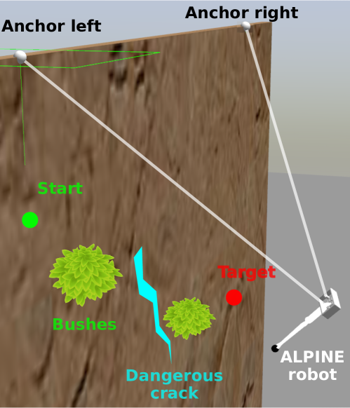
The ALPINE robot proposed in this paper hangs on two ropes, which make it able to carry heavy workloads (e.g., equipments to execute maintenance operations) and to remain in stationary position with a negligible amount of energy by setting the brakes on the rope (R1). To satisfy R2, the robot exploits two ropes (which can pull the structure up-wards and sustain its weight) and a prismatic leg that can extend and retract quickly to make the robot jump away from the slope. During the jump and the flight phase, the ropes are independently wound/unwound to control the robot trajectory. The flight is stabilised using the thrust of an auxiliary rotor propeller. The combination of jumps and mixed vertical/lateral motion is energetically efficient and enables quick motion. In fact, rather than slowly taking steps as walking/sticking mechanisms, the robot can take one or multiple and fast jumps, like Salto-1P [28], and employ the winding/unwinding mechanism to reach the desired locations. The paper proposes motion planning and control strategies to travel around obstacles (R3), as shown in Fig. 2. The adoption of a simplified model of the system allows us to solve the multi-jump motion planning and control problem with efficient numeric approaches. A landing mechanism allows the robot to dissipate the excess of kinetic energy and stay firm on the wall while executing tasks. This feature, along with an appropriate design of the planning and control components, delivers a good degree of flexibility in the operation mode (R4).

Scientific challenges. The first scientific challenge of the ALPINE robot lies in its under-actuation: it is impossible to fully control the robot’s Center of Mass (CoM) when not in contact with the wall. Second, one of the actuators (the leg) operates in an impulsive way, while the ropes can only operate in the pulling direction (unilateral actuation). The problem is partially alleviated by the auxiliary propeller during the flight phase, but the resulting system dynamics is hybrid (the continuous evolution is interpersed with discrete changes). As regards motion planning, since the motion of the robot depends on both the impulse exerted on the wall and the winding/unwinding of the ropes, a successful strategy should consider the combined effects of under-actuation, rope constraints, the actuator limits and the contact interaction (i.e., friction). Whilst numeric optimisation is certainly a powerful tool [29, 34], the combination of these factors and hybrid dynamics, makes the problem tractability far from obvious. Paper Contribution and Summary. The contributions of the paper can be summarised as follows. i) The conceptual design of the jumping robot platform ALPINE (Section 2); ii) a reduced-order model to simplify the solution of optimal control strategies (Section 2); iii) a static analysis to evaluate the maximum value of operating forces that the system is able to withstand in the execution of its tasks (Section 3); iv) A computationally efficient planning algorithm to generate a jump to reach desired targets while overcoming obstacles (Section 4); v) a motion control strategy to track the reference trajectories with high landing accuracy (Section 5). The efficacy of the system design, as well as of motion planning and control, is tested in a large set of physical simulations (Section 6). In Section 7, we offer our conclusion and announce future work directions.

Figure 2: Realistic Gazebo simulation of ALPINE during a jump.

A very preliminary sketch of the robot (with only one rope) was already presented in [22]. We go beyond that contribution extending it to two ropes, adding motion control and landing features and providing a static analysis and performing extensive simulations.

2 Robot Modeling

As mentioned above, a robot hanging on a rope has the ability to preserve energy when static by simply engaging the brakes in the hoist. However, a robot hanging on a single rope [22, 26] has severe limitations in terms of possible lateral motions, and hence reachable locations. Additionally, the lateral pull of the rope makes the system unstable when static, limiting its ability to execute tasks. A possible way to tackle these issues is to have an additional prismatic joint (a slider) that enables the motion of the rope anchor point. While easy to control, this solution requires that the slider be mounted on a path clear from obstacles, which is difficult in environments where rock protrusions and bushes are common.

With these limitations in mind, we opted for a different design based on a second rope attached to an additional fixed anchor on the wall. Both ropes can be independently wound/unwound by means of hoist motors (see Fig. 4). Deploying the two anchors independently removes the limitation of having a clear path for the slider, while the mechanical design is significantly simplified. Another advantage is an increased robustness to disturbances coming from the operations, as detailed in Section 3. The price to pay is a higher control complexity, since the release/winding of the ropes needs to be accurately coordinated.

2.1 Full robot model

We model the robot as 3 kinematic chains branching from the base link (see Fig. 3).

Figure 3: Topology of the joints for the full detail model. Links are red boxes and joints blue circles (revolute) or blue boxes (prismatic). Shaded joints are the passive ones, not shaded ones are the active ones.

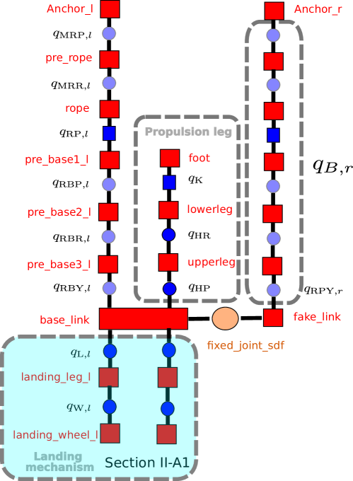
One chain represents the propulsion mechanism (a 3-DoF prismatic leg) [22]: at the extreme of the leg there is a point-like foot. The leg is also endowed with two adjacent rotational joints, called hip pitch ($q_{HP}$, rotating about the base $Y$ axis) and hip roll ($q_{HR}$, rotating about the base $X$ axis). These joints are needed to align the leg to the thrusting impulse, so as to avoid the generation of centroidal moments that would pivot the robot around the rope axis. A prismatic knee joint ($q_{K}$) is used to generate the thrusting impulsive force. The landing mechanism is represented by two additional rotational joints that move the landing links (see Fig. 5) with two passive wheels at the extreme as described in more detail in Section 2.1.1.

The other two kinematic chains model the two ropes. To host the hoist motors, the attachment points of the ropes are mounted with an offset $d_{h}/2$ w.r.t. the base frame (see Fig. 4). We model the attachment between each anchor and the corresponding rope by 2 passive (rotational) joints. Each rope can be seen as an actuated prismatic joint ($q_{RP,l}$ or $q_{RP,r}$), followed by 3 passive rotational joints to model the connection between the rope and the base link (see also Fig. 4).

Figure 4: Kinematic model of the ALPINE robot; solution with two ropes (standard definitions). A propeller is mounted on the rear of the robot. The inertial ($\mathcal{W}$) frame is attached to the left anchor frame.

The described mounting choice is indeed equivalent to allocating $3$ joints at the anchor point and $2$ at the base. However, to avoid a redundant representation, there must be only one passive rotational joint aligned with the rope. To increase the robot controllability (e.g. capability to apply forces on the base) along the direction perpendicular to the ropes plane, we added a propeller mounted on the back of the base link, as depicted in Fig. 4. This brings several advantages. First, it allows the robot to reject disturbances and tracking errors in the direction perpendicular to the ropes plane, enhancing controllability. Second, it increases the maximum force the robot can withstand during operations without losing contact. This is particularly relevant when dealing with harder rocks: by activating the propellers to provide additional push against the walls, we can increase the force margin available for operations, such as drilling. Lastly, it enables the control of the orientation by actuating the propellers in a differential way. In this paper, we will focus on exploiting only the disturbance rejection feature, leaving the other two features for future work.

Neglecting the $4$ joints of the landing mechanism (see Section 2.1.1) and the propeller, the total number of Degrees of Freedom (DoFs) is $n=15$, represented by the configuration vector $\mathbf{q}\in\mathbb{R}^{15}$. Ten of these joints are relative to the attachment of the ropes to the hoist and the anchor and are passive. Fig. 3 illustrates the joint definitions: $MRX$ (Mountain Rope X = Pitch/Roll), $RP$ (Rope Prismatic) and $RBX$ (Rope Base X = Roll/Pitch/Yaw). By stacking the different joint variables related to the left rope, we obtain the vector $\mathbf{q}_{B,l}=\begin{bmatrix}q_{MRP}&q_{MRR}&q_{RP}&q_{RBP}&q_{RBR}&q_{RBY}\end{bmatrix}^{T}$. We can repeat the same for the right rope stacking the joint variable into the vector $\mathbf{q}_{B,r}$ and come up with the definition of the joint state $\mathbf{q}=\begin{bmatrix}\mathbf{q}_{B,l}^{T}&\mathbf{q}_{B,r}^{T}&q_{HP}&q_{HR}&q_{K}\end{bmatrix}^{T}$, where additionally we have $HX$ (Hip X = roll/pitch) and $K$ (Knee) joints. The dynamic equation of motion is subject to a holonomic constraint because the two attachment points $\mathbf{p}_{h,l}(\mathbf{q})$, $\mathbf{p}_{h,r}(\mathbf{q})$ are located at a fixed distance $d_{h}$, i.e.

$$\|\mathbf{p}_{h,l}(\mathbf{q})-\mathbf{p}_{h,r}(\mathbf{q})\|^{2}=d_{h}^{2}.$$ (1)

This description creates a kinematic loop represented by the trapezoid having the two ropes as edges. The full dynamic equation is reported here just for reference

$$\begin{cases}&\mathbf{M}(\mathbf{q})\mathbf{\ddot{q}}+\mathbf{h}(\mathbf{q},\mathbf{\dot{q}})=\begin{bmatrix}\mathbf{0}_{10\times 1}\\ \bm{\tau}_{a}\end{bmatrix}+\mathbf{J}_{c}(\mathbf{q})^{T}\mathbf{f}_{c}+\mathbf{J}_{p}(\mathbf{q})^{T}f_{p},\\ &\mathbf{A}(\mathbf{q})\dot{\mathbf{q}}=\mathbf{0},\\ &\tau_{RP,l}\geq 0,\\ &\tau_{RP,r}\geq 0,\end{cases}$$ (2)

where $\mathbf{M}\in\mathbb{R}^{n\times n}$ is the inertia matrix, $\mathbf{h}\in\mathbb{R}^{n}$ represents the bias terms (Centrifugal, Coriolis and Gravity), and $\mathbf{J_{c}}\in\mathbb{R}^{3\times n}$ is the Jacobian relative to the prismatic leg contact point (foot) that maps the contact force $\mathbf{f}_{c}\in\mathbb{R}^{3}$ into the generalised coordinate space. $f_{p}\in\mathbb{R}$ is a scalar and represents the magnitude of the propeller force that is mapped into the robot dynamics through $\mathbf{J}_{p}(\mathbf{q})=\mathbf{\hat{x}}_{b}^{T}\mathbf{J}_{b}(\mathbf{q})\in\mathbb{R}^{1\times n}$, where $\mathbf{\hat{x}}_{b}$ is the $X$ asis of the base link and $\mathbf{J}_{b}(\mathbf{q})=\begin{bmatrix}\frac{\partial\mathbf{p}(\mathbf{q})}{\partial\mathbf{q}}\end{bmatrix}\in\mathbb{R}^{3\times n}$ is the Jacobian of the robot base. The $\mathbf{A}(\mathbf{q})\dot{\mathbf{q}}=\mathbf{0}$ constraint is (1) rewritten at the velocity level. The force/torque variable of the the actuated joints are grouped into the vector $\bm{\tau}_{a}=\begin{bmatrix}\bm{\tau}_{RP,l}&\bm{\tau}_{RP,r}&\bm{\tau}_{\text{leg}}\end{bmatrix}^{T}\in\mathbb{R}^{5}$. We will employ the right hand side of (2) to express the mapping of the contact force and of the propeller force into joint torques.

2.1.1 Landing Mechanism

The robot in Fig. 4 would not be able to self-stabilise on the wall with a single leg, therefore we designed a landing mechanism, depicted in Fig. 5, formed by two additional rotational joints $q_{L,l}$ and $q_{L,r}$ located on the sides of the base link allowing to activate two landing legs.

Figure 5: Overview of the landing mechanism, with joint and variable definitions. $d_{w}$ and $d_{b}$ are the wall clearance and base line parameters. Passive wheels are attached to the extremes of the landing legs.

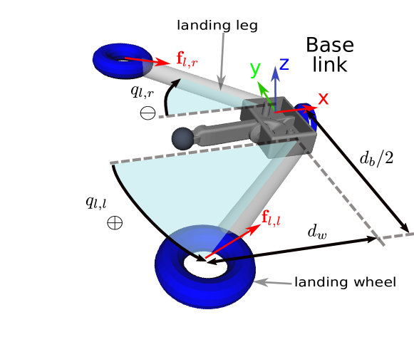
Moreover, we added two wheels at the tips of the landing legs, which can move laterally during the contact and, hence, avoid the generation of internal forces (i.e., non perpendicular to the wall).

2.2 Reduced-order model with minimal representation

The high number of states and the constraint in (2) makes the full dynamics hardly tractable for control design. For this reason, we derive a lower dimensional (reduced-order) model with only $3$ DoFs that captures the dominant dynamics of the system along with the holonomic kinematic constraint (1). To this end, we make the following simplifying assumptions: 1) the mass is entirely concentrated in the body attached to the rope and we neglect the angular dynamics and 2) during the winding/rewinding of the ropes they remain completely elongated (i.e., they are not bending).

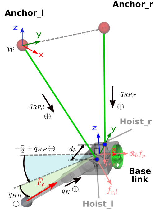
In order to simplify the control design, we approximate the rope attachment points as coincident and then choose a minimal representation for the state with $3$ DoFs. Specifically, the reduced state $\mathbf{q}_{r}$ is defined as $\mathbf{q}_{r}=\begin{bmatrix}\psi&l_{1}&l_{2}\end{bmatrix}\in\mathbb{R}^{3}$, where $\psi$ is the angle formed from the ropes plane and the wall, and $l_{1}$, $l_{2}$ the length of the left and right ropes, respectively. A geometric scheme of the reduced model with vector definitions is shown in Fig. 6.

Figure 6: Reduced order model with two anchor points: standard definitions (left) and side view (right). The impulsive force $\mathbf{f}_{\text{leg}}$ is applied only when the leg is in contact.

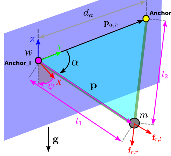
Assuming the inertial frame $\mathcal{W}$ attached to the left anchor point, the dynamics of the point $\mathbf{p}$ (where the robot mass is concentrated, by assumption) is defined by the Newton Equation:

$$m(\mathbf{\ddot{p}}-\mathbf{g})=\underbrace{\mathbf{\hat{f}_{r,l}}f_{r,l}}_{\mathbf{f}_{r,l}}+\underbrace{\mathbf{\hat{f}_{r,r}}f_{r,r}}_{\mathbf{f}_{r,l}}+\mathbf{f}_{leg}+\mathbf{n}_{\perp}f_{p},$$ (3)

where $\mathbf{\hat{f}_{r,i}}=\frac{\mathbf{p}-\mathbf{p}_{a,i}}{\|\mathbf{p}-\mathbf{p}_{a,i}\|}\in\mathbb{R}^{3}$ and $f_{r,i}\in\mathbb{R}$, with $i=\{r,l\}$, are the rope axes and the magnitude of the exerted forces, respectively. The term $\mathbf{n}_{\perp}f_{p}$ represents the propeller’s force where $\mathbf{n}_{\perp}\in\mathbb{R}^{3}$ is the unit vectors perpendicular to the ropes plane.

The two anchor point positions are given by $\mathbf{p}_{a,l}$ and $\mathbf{p}_{a,r}$. The input variables are: 1) the rope forces $\mathbf{f}_{r,i}$ oriented along the rope axes; 2) an impulsive pushing force $\mathbf{f}_{\text{leg}}$ (applied at $\mathbf{p}$) that the robot generates when in contact with the mountain (see Fig. 6). Therefore, the expression of the forward kinematics for the position $\mathbf{p}$ of the robot (origin of the base-link) as a function of $\mathbf{q}_{r}$ is given by:

$$\mathbf{p}(\mathbf{q}_{r})=\begin{bmatrix}l_{1}\sin(\psi)\sqrt{1-\frac{(d_{a}^{2}+l_{1}^{2}-l_{2}^{2})^{2}}{4d_{a}^{2}l_{1}^{2}}}\\ (d_{a}^{2}+l_{1}^{2}-l_{2}^{2})/(2d_{a})\\ -l_{1}\cos(\psi)\sqrt{1-\frac{(d_{a}^{2}+l_{1}^{2}-l_{2}^{2})^{2}}{4d_{a}^{2}l_{1}^{2}}}\end{bmatrix},$$ (4)

where the holonomic constraint (1) has been embedded and $d_{a}$ is the distance between the anchors. The dynamics of the point mass as defined in (3) is given by the second derivative of (4), which gives an implicit expression for the coupled derivatives $\ddot{\psi}$, $\ddot{l_{1}}$ and $\ddot{l_{2}}$, thus leading to the following matrix form of (3)

$$m\underbrace{\left(\mathbf{A}_{d}\begin{bmatrix}\ddot{\psi}\\ \ddot{l}_{1}\\ \ddot{l}_{2}\end{bmatrix}+\mathbf{b}_{d}\right)}_{\ddot{\mathbf{p}}}=\underbrace{m\mathbf{g}+\mathbf{f}_{leg}+\mathbf{J}_{r}\begin{bmatrix}f_{r,l}\\ f_{r,r}\end{bmatrix}+\mathbf{n}_{\perp}f_{p}}_{\mathbf{f}_{tot}},$$ (5)

where $\mathbf{A}_{d}$ and $\mathbf{b}_{d}$ are reported in the Appendix, and $\mathbf{J}_{r}=\begin{bmatrix}\hat{\mathbf{f}}_{r,l}&\hat{\mathbf{f}}_{r,r}\end{bmatrix}\in\mathbb{R}^{3\times 2}$. Finally, we obtain:

$$\begin{bmatrix}\ddot{\psi}\\ \ddot{l}_{1}\\ \ddot{l}_{2}\end{bmatrix}=\mathbf{A}_{d}^{-1}\left[\frac{1}{m}\mathbf{f}_{tot}-\mathbf{b}_{d}\right].$$ (6)

Note that this model has a singularity when the term $\sin(\psi)$ in $\mathbf{A}_{d}$ becomes zero. The configuration $\psi=0$ corresponds to the robot base lying on the vertical wall, which never happens if the ropes are connected directly (i.e., without obstacles in between) to the robot base, due to the presence of the leg. For over-hanging walls, no rope-based system can be employed because the contact cannot be ensured nor maintained.

3 Static Analysis

3.1 Feasible Polytope

In this section we present a numerical procedure to evaluate the static stability of the robot for a set of locations once landed on the wall. Since the robot with only one leg would be inherently unstable on the wall, we consider the ensemble robot and landing mechanism. The analysis aims to answer the following queries: (Q1) Is it possible to find a static balance between gravity, rope tensions and forces at the landing wheels for a given position that allows the robot to remain in contact with the wall? The presence of this equilibrium is key to the execution of any robot task. (Q2) How do the limits on the actuators and the presence of external forces affect static stability? More generally, for each robot location on the wall it is important to evaluate the maximum operation forces that can be generated. Both aspects are fundamental to execute any task, since the contact forces generated for maintenance operation (called operation forces) must be balanced by the landing wheels and by the ropes. For instance, if operation forces required a force on the feet violating the unilateral condition, the robot will tip over. To answer Q2 we consider unilaterality, friction and actuation constraints, while to answer Q1 only unilaterality and friction are sufficient.

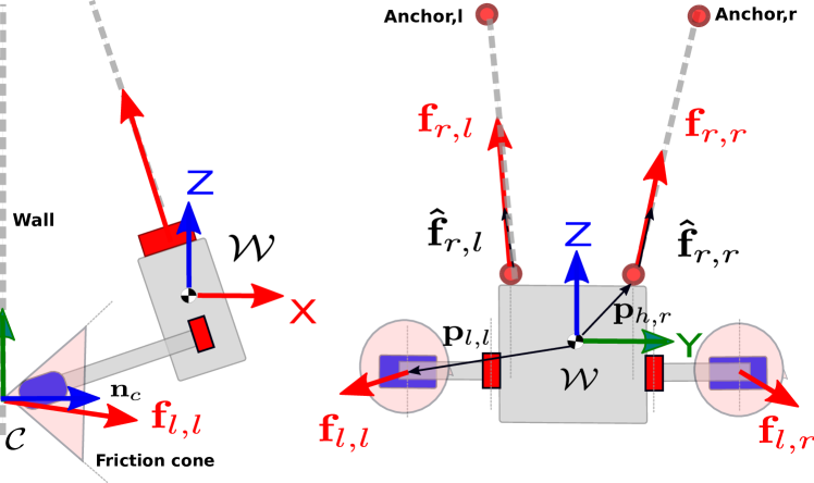
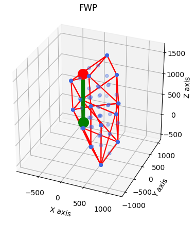
The following assumptions underlie the present analysis: 1) we approximate the assembly robot+landing mechanism as a rigid body which is in contact with the wall with the landing wheels; 2) we neglect the masses of the legs of the landing mechanism; 3) we assume that the contact forces for the landing wheels are linear forces (i.e. point-feet contacts) limited by the unilateral and friction cone constraints. For this analysis we introduce the concept of Feasible Wrench Polytope (FWP) [35] and we refer to Fig. 7 for standard definitions.

Figure 7: Definition of vectors and frames for the rigid body model used in the static analysis: (left) side view (right) front view. Differently from Section 2, the inertial frame W is attached to the CoM.

The FWP represents the set of feasible wrenches at the centroid (i.e., forces and moments) than can be tolerated while satisfying 1) the balance equation of forces under the action of gravity (static condition), 2) unilateral conditions of the contacts, 3) friction constraints and 4) actuation limits. Therefore, the feasible wrenches can be seen as a compact representation of the mentioned constraints 1-4 projected at the CoM by means of a Minkowski sum operation.

Proceeding with the computation of the FWP [35], the first step is to compute the Force polytopes $\mathcal{F}_{i}$ associated with the feet and rope forces. We define $n_{c}=4$ unilateral contacts, two at the landing wheels and two at the rope attachment points with the base (refer to Fig. 7). In the case of the landing wheels, friction constraints are present while the ropes have an additional constraint on the direction: namely, the force has to be acting along the rope axis. Adopting an approximation that is commonplace in robotics, we (conservatively) approximate the cone constraint with an inner pyramid and bound them along the normal direction with the maximum $f_{max}$. Note that the friction cone implicitly encodes also the unilateral constraint ($\mathbf{n}_{c}^{T}\mathbf{f}_{l,i}>0$). This way, we encode in a single matrix of constraints: unilaterality, friction and actuation bound for the $i$-th wheel. The vertices of the obtained force polytope are stored as columns:

$$\mathbf{f}^{\lim}_{l,i}={}_{\mathcal{W}}\mathbf{R}_{c}(\mathbf{n}_{c})\begin{bmatrix}0&\mu&-\mu&-\mu&\mu\\ 0&\mu&\mu&-\mu&-\mu\\ 0&1&1&1&1\end{bmatrix}f_{\mathrm{leg},\max},i\in\{l,r\},$$ (7)

where ${}_{\mathcal{W}}\mathbf{R}_{c}$ is the rotation matrix related to the contact frame $\mathcal{C}$ and $f_{\mathrm{leg},\max}$ is the maximum force in the normal direction $\mathbf{n}_{c}$. Regarding the rope forces, they are constrained to lie on a mono-dimensional manifold (i.e. along the axis $\mathbf{\hat{f}}_{r,i}$) and subject to unilateral ($f_{r,i}<0$) and actuation constraints ($-f_{r,i}^{\max}\leq f_{r,i}$). Then the Force Polytope associated to rope $i$ boils down to a segment with only two vertices:

$$\mathbf{f}^{\lim}_{r,i}=\begin{bmatrix}-\mathbf{\hat{f}}_{r,i}&\mathbf{0}_{3\times 1}\end{bmatrix}f_{r,\max},$$ (8)

Next, for each vertex, we add the moments that are generated in correspondence to the maximum forces:

$$\mathbf{w}_{l,i}=\begin{bmatrix}\dots\mathbf{f}^{\lim}_{l,i,k}\dots\\ \dots\mathbf{p}_{l,i}\times\mathbf{f}^{\lim}_{l,i,k}\dots\end{bmatrix}\quad\text{with }k=1,\dots,5,$$ (9)

where $\mathbf{p}_{l,i}\in\mathbb{R}^{3}$ represents the position of the $i$-th landing wheel and $\mathbf{w}_{l,i,k}\in\mathbb{R}^{6}$ represents a wrench that can be realized at that wheel. Likewise, for ropes:

$$\mathbf{w}_{r,i}=\begin{bmatrix}-\mathbf{\hat{f}}_{r,i}&\mathbf{0}_{3\times 1}\\ -\mathbf{p}_{h,i}\times\mathbf{\hat{f}}_{r,k}&\mathbf{0}_{3\times 1}\end{bmatrix}f_{r,\max},$$ (10)

where $\mathbf{p}_{h,i}\in\mathbb{R}^{3}$ is the $i$-th rope attachment point. Therefore, the set of admissible wrenches that can be applied at the CoM by the $i-{th}$ wheel is:

$$\mathcal{W}_{l,i}=ConvexHull(\mathbf{w}_{l,i,1},\dots,\mathbf{w}_{l,i,5}),\quad i\in\{l,r\}.$$ (11)

The convex hull operation should be performed also for ropes to compute $\mathcal{W}_{r,i}$ and has the purpose to eliminate internal vertices. We now have $n_{c}=4$ wrench polytopes $\mathcal{W}_{i}$ that contain all the admissible wrenches that can be applied to the robot’s CoM.

Finally, the FWP is computed through the Minkowski sum of the $\mathcal{W}_{i}$ for all the contacts:

$$FWP=\oplus_{i=1}^{n_{c}}\mathcal{W}_{i}.$$ (12)

Since we used a vertex description ($\mathcal{V}$-description), the Minkowski sum can be efficiently obtained as in [36]. Remark: To avoid polytopes becoming flat it is preferable to define all quantities w.r.t. an inertial frame placed in a location different from the anchors. More precisely, it is convenient to refer all quantities about the CoM (see Fig. 7). Henceforth, only for this section, we assume that the inertial frame is attached to the CoM and not to the left anchor. In a preliminary analysis, to answer Q1, we assume there are no actuation limits. The FWP, in this case becomes unbounded, and becomes a Contact Wrench Cone (CWC) [37]. We define a robot position feasible if there exists a set of rope and wheel forces that 1) ensures static equilibrium, 2) ensures unilateral and friction constraints.

3.2 Gravitational wrench

To evaluate the feasibility of a robot location, we first compute the gravito-inertial wrench $\mathbf{w}_{G}$ in the specific robot state. Because we are dealing with a static analysis we neglect the inertial effects:

$$\mathbf{w}_{G}=\begin{bmatrix}m\mathbf{g}\\ \mathbf{p}\times m\mathbf{g}\end{bmatrix},$$ (13)

where $\mathbf{p}$ is the robot CoM position (equal to $\mathbf{0}$ because the inertial frame is attached to the CoM). A feasibility criterion can be written as:

$$\mathbf{w}_{G}\in FWP.$$ (14)

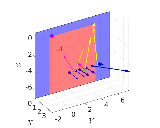
The criterion (14) tells us that it exists a feasible set of forces $\begin{bmatrix}(\hat{\mathbf{f}}_{r,l}f_{r,l}),(\hat{\mathbf{f}}_{r,r}f_{r,r}),\mathbf{f}_{l,l},\mathbf{f}_{l,r}\end{bmatrix}$ that generates the wrench $\mathbf{w}_{G}$. We evaluate (14) at different positions on the wall, on a fine grid. We set a friction coefficient of $\mu=0.8$, a distance of the anchors $d_{a}=5$ m, the relative distance of the landing wheels $d_{b}=0.8$ m and the wall clearance $d_{w}=0.4$ m (see Fig. 5). The outcome of this analysis is that the set of equilibrium locations on the wall is mostly limited to the rectangle delimited by two anchors (red shaded area $\mathcal{A}$ in Fig. 8).

Figure 8: Results of the static analysis in three representative points for $\mathbf{p}_{z}=5$ m. The red shaded area $\mathcal{A}$ indicates all the robot positions for which static equilibrium, unilateral and friction constraints are fulfilled. We report the forces for 3 representative robot positions. The figure shows that, the rope connected to the closer anchor point gets gradually loaded when moving towards it, while the rope connected to the farther anchor gets gradually unloaded.

To answer Q2, we are interested in the additional operation forces that can be tolerated when the robot is in equilibrium, for which we want to evaluate the operating margin. This time, we also consider actuation limits, and find that the answer is closely correlated to the concept of feasibility margin, which can be computed from the FWP. The feasibility margin of applicable operating forces is defined as the smallest distance between the gravitational wrench $\mathbf{w}_{G}$ and the boundaries represented by the FWP facets. Authors in [35] show that an estimate of this margin could be obtained directly from the vertex ($\mathcal{V}$) description. However, a margin computed with the vertex description is a normalised value. Additionally, we might be interested in evaluating the maximum wrench and then the relative margin in a specific direction $\hat{\mathbf{v}}\in\mathbb{R}^{6}$. In this case the vertex description is no longer sufficient, and we ought to derive the half-plane (i.e. $\mathcal{H}$-description) of the FWP from the $\mathcal{V}$-description via the double description algorithm [38]. In the $\mathcal{H}$-description, the FWP set can be written in terms of half-spaces as:

$$FWP=\{\mathbf{w}\in\mathbb{R}^{6}|\hat{\mathbf{a}}_{j}^{T}\mathbf{w}\leq\mathbf{0},j=1,\dots n_{h}\},$$ (15)

where $n_{h}$ is the number of half-spaces of the FWP and $\hat{\mathbf{a}}_{j}\in\mathbb{R}^{6}$ is the normal vector to the j-th facet. The feasibility criterion expressed in (14) can thus be formulated as:

$$\mathbf{A}_{p}\mathbf{w}_{G}\leq\mathbf{b}_{p},$$ (16)

where $\mathbf{A}_{p}\in\mathbb{R}^{n_{h}\times 6}$ is the matrix whose rows are $\hat{\mathbf{a}}_{j}$.

3.3 Evaluating the feasibility margin

The feasibility margin $\gamma\in\mathbb{R}$ in the direction $\hat{\mathbf{v}}$ is the distance (along $\hat{\mathbf{v}}$) between $\mathbf{w}_{G}$ and the polytope boundary and can be obtained by solving the following Linear Program (LP):

$$\gamma^{\star}=\operatorname*{\arg\!\min}_{\gamma} -\gamma$$ (17a)

s.t. $$\mathbf{A}_{p}(\mathbf{w}_{G}+\gamma\mathbf{\hat{v}})\leq\mathbf{b}_{p},$$ (17b)

Hereby, (17b) ensures that the total wrench $\mathbf{w}_{G}+\gamma\hat{v}$ is inside the FWP set.

Figure 9: Representation of the linear part of the FWP computed for a position $\mathbf{p}=[1.5,2.5,-6.5]^{T}$. The green point is the gravitational wrench $\mathbf{w}_{G}$. The red point is the maximum wrench along the direction $\hat{\mathbf{v}}$ (green line).

The solution $\gamma^{\star}$ of (17) gives the surplus of additional external wrench $\gamma^{\star}\mathbf{\hat{v}}$ that can be tolerated by the system [35]. We illustrate in Fig. 9 a 3D representation of the linear part of the FWP computed for a position $\mathbf{p}=\begin{bmatrix}1.5&2.5&-6.5\end{bmatrix}^{T}$.

3.4 Numeric evaluation

In a first representative operation that ensembles a drilling operation, we compute the feasibility margin to generate a pure force (i.e. passing through the CoM) along the $X$ direction $\hat{\mathbf{v}}=\begin{bmatrix}-1&0&0&0&0&0\end{bmatrix}^{T}$ for robot positions with $Y$ ranging between the two anchors (i.e. from $0$ to $5$ m) and the $Z$ component ranging from $-2$ to $-10$ m. We repeat the analysis for two different wall inclinations (0.2 and 0.4 rad) that will result in different $\mathbf{n}_{c}$. To have the robot in contact, the $X$ component is set to $1.7$ and $3$ m, respectively. Figure 10 (left plots) reports the 2D (heat-map) representation of the value of the feasibility margin for the two different wall inclinations. The friction coefficient is set to $\mu=0.8$.

Figure 10: Heat-maps of the feasibility margin computed for different positions along the wall, (left plots) along $-\mathbf{f}_{x}=[-1,0,0,0,0,0]^{T}$ for a drilling application, for a wall inclination of 0.2 rad (first), and 0.4 rad (second) and (right plots) along $-\mathbf{f}_{z}=[0,0,-1,0,0,0]^{T}$ (third) and $\mathbf{m}_{y}=[0,0,0,0,-1,0]^{T}$ direction (fourth) relative to a debris removal operation which involves the application of a not purely centroidal force (also a moment). In the third plot we reported the results for 3 values of the friction coefficient $\mu=\{0.4,0.6,0.8\}$. The feasibility margin is a synthetic metric to estimate the amount of external forces and moments available for operations. We report the absolute value of the margin $\gamma$.

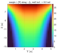
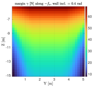
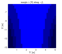
As expected, the margin decreases with the distance to the anchors because the angle $\psi$ decreases with rope elongation (for the same wall clearance), and pushing on the wall becomes more difficult because the legs get more and more unloaded. For the same reason, a more slanted wall involves overall higher gravity components and, hence, overall more feet loading, thus higher values for the margin can be observed. The diagonal shape is related to the friction constraint which is violated in the dark blue area. In these cases the whole static feasibility is invalidated (i.e. $\mathbf{w}_{G}$ goes out of the polytope) and we set the margin to be null.

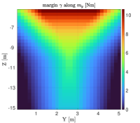
In a second analysis (see Fig. 10, right plots) we consider a composite loading as observed in a debris removal application, pictorially represented in Fig. 1, middle. This time we consider a purely vertical wall (i.e. $\mathbf{n}_{c}=\begin{bmatrix}1&0&0\end{bmatrix}^{T}$) with a constant $\mathbf{p}_{x}=1.5$ m. Interestingly, for the margin in the vertical direction, only two values are possible: zero in the region for which friction constraints are violated (we did a parametric analysis for $\mu=\{0.4,0.6,0.8\}$ to highlight its influence), and the value of the gravity ($147$ N) in the remaining region. This means that the vertical push is obtained through the action of gravity and cannot go beyond that. We also noticed that the position of the feet is fundamental to achieve a stable configuration (i.e. they cannot be shifted too much w.r.t the CoM in the vertical direction, cf. Fig 7). The results for the moment $\mathbf{m_{y}}$ (fourth plot) are more inline with the $\mathbf{f}_{x}$ case, where higher margins are related to positions between the anchors. This is a quantitative evaluation that is important for real operations: being able to evaluate the operating margin is a feature useful to optimise costs-related drilling operations depending on the type of the rock. For instance, to perform a $10$ cm drilling operation on hard rock, a high force could be applied for a short time, or a low force for a long time. Being able to estimate the maximum force applicable gives benefits in terms of cost effectiveness, because it allows to minimise the time budget for the operation.

4 Motion Planning

Setting up a navigation approach for the ALPINE robot is a non-trivial task. First of all, even the simplified dynamics (6) is highly nonlinear. Second, the configurations between which the robot moves are usually distant, and therefore, linearising the dynamics around an operating point would lead to inaccurate results. Third, one of the inputs, the thrusting force $\mathbf{f}_{\text{leg}}$, has an impulsive nature, operating at discrete time instants, and its tangential component is constrained by friction. Therefore, it is not possible to use it in any feedback control scheme.

As customary in robotics, we split the navigation problem into two sub-problems: 1) motion planning, i.e., deciding a trajectory before the motion starts, 2) motion control, i.e., a feedback controller that operates the rope/propeller forces to compensate for small deviations to track the trajectory and land in proximity of the expected position. This section focuses on step 1 and considers the robot without the landing mechanism. The motion plan for the robot is decided by solving a nonlinear optimal control problem (OCP), which in general is modelled as follows:

$$\min_{\mathbf{x}(t),\mathbf{u}(t)} \,\,m_{f}(\mathbf{x}(t_{f}))+\int_{0}^{t_{f}}l\left(\mathbf{x}(t),\mathbf{u}(t)\right)dt,$$ (18a)

s.t.

$$\,\,\dot{\mathbf{x}}(t)=\mathbf{f}(\mathbf{x}(t),\mathbf{u}(t)),$$ (18b)

$$\,\,\mathbf{u}(t)\in\mathcal{U},$$ (18c)

$$\,\,\mathbf{h}\left(\mathbf{x}(t),\mathbf{u}(t)\right)\leq 0,$$ (18d)

$$\,\,\mathbf{B}(\mathbf{x}(t_{0}),\mathbf{x}(t_{f}))=0,$$ (18e)

where $l(\mathbf{x},\mathbf{u})$ and $m_{f}(\mathbf{x})$ are the running and the terminal costs, $\mathbf{x}$ is state, $\mathbf{U}$ is the control input constrained in the convex set $\mathcal{U}$, $\mathbf{f}$ is the dynamics, $\mathbf{h}$ are the path constraints, and $\mathbf{B}$ are the boundary conditions. To reduce the computational effort, we consider as $\mathbf{f}$ the reduced-order model (6), which implicitly includes the closed-loop kinematic constraints. The control inputs should include both the rope forces $\mathbf{u}=\begin{bmatrix}f_{r,l},f_{r,r}\end{bmatrix}\in\mathbb{R}^{2}$ and the leg impulse. However, the latter is applied only during the thrusting phase, which typically lasts a short amount of time $t_{\text{th}}\in\mathbb{R}$. For this reason, we assume it remains constant during this phase, and treat it as an additional state with null dynamics. As decision variables, we consider: 1) the vector of control inputs $\mathbf{U}=\begin{bmatrix}\mathbf{F}_{r,l},\mathbf{F}_{r,r}\end{bmatrix}$ where $\mathbf{F}_{r,l},\mathbf{F}_{r,r}$ are the trajectories of the rope forces along the horizon, 2) the horizon length $t_{f}\in\mathbb{R}$, and 3) the initial leg impulse $\mathbf{f}_{\text{leg}}\in\mathbb{R}^{3}$.

System Dynamics. Because we define a priori the duration of the thrusting phase, the dynamics of our system is time-varying. When the leg is in contact, the dynamics accounts for the force $\mathbf{f}_{\mathrm{leg}}(t)$ generated by the thrusting leg. Rather than modeling this force as an impulse, we model it as:

$$\mathbf{f}_{\mathrm{leg}}(t)=\begin{cases}\mathbf{f}_{\mathrm{leg}}\quad 0\leq t\leq t_{\text{th}},\\ \mathbf{0}_{3\times 1}\quad t>t_{\text{th}}.\end{cases}$$ (19)

Hence, during the contact $t\in\begin{bmatrix}0&t_{\text{th}}\end{bmatrix}$, the leg applies a constant force $\mathbf{f}_{leg}$ while, for $t\in\begin{bmatrix}t_{\text{th}}&t_{f}\end{bmatrix}$, this force is zero. Given the nature of our actuation mechanism, a realistic choice is to have a duration in the order of tens of milliseconds, which consequently determines a remarkable intensity of the impulse. We incorporate the leg force $\mathbf{f_{\text{leg}}}(t)$ in the state vector $\mathbf{x}$ with a null dynamics. The state of our problem, hence, is defined as:

$$\mathbf{x}=\begin{bmatrix}\psi&l_{1}&l_{2}&\dot{\psi}&\dot{l_{1}}&\dot{l_{2}}&\mathbf{f}_{\text{leg}}^{T}\end{bmatrix}^{T}\in\mathbb{R}^{9}.$$ (20)

However, when the contact is broken at $t=t_{th}$, the variable $\mathbf{f}_{\text{leg}}$ must disappear from the state. We model this change in state dimension by defining a matrix $\mathbf{S}$ that selects the first 6 elements the 9D state vector:

$$\begin{array}[]{ll}\mathbf{x}^{+}=\mathbf{S}\,\mathbf{x},&t=t_{th},\end{array}$$ (22)

Consequently, the state-space representation of the nonlinear dynamics, casted in input-affine form, can be derived from (6):

$$\begin{array}[]{ll}\dot{\mathbf{x}}=\mathbf{f}_{leg}(\mathbf{x})+\mathbf{g}_{leg}(\mathbf{x})\mathbf{u},&t<t_{\text{th}},\\ \dot{\mathbf{x}}=\mathbf{f}_{noleg}(\mathbf{x})+\mathbf{g}_{noleg}(\mathbf{x})\mathbf{u},&t>t_{\text{th}},\end{array}$$ (25)

where:

$$\mathbf{f}_{leg}(\mathbf{x})=\begin{bmatrix}\mathbf{x}_{4\dots 6}\\ \mathbf{A}_{d}^{-1}\left[\frac{\mathbf{x}_{7\dots 9}}{m}+\mathbf{g}-\mathbf{b}_{d}\right]\\ \mathbf{0}_{3\times 1}\end{bmatrix}$$ (26)

$$\mathbf{g}_{leg}(\mathbf{x})=\begin{bmatrix}\mathbf{g}_{noleg}(\mathbf{x})\\ \mathbf{0}_{3\times 2}\end{bmatrix}$$ (27)

$$\mathbf{f}_{noleg}(\mathbf{x})=\begin{bmatrix}\mathbf{x}_{4\dots 6}\\ \mathbf{A}_{d}^{-1}\left(\mathbf{g}-\mathbf{b}_{d}\right)\\ \end{bmatrix}$$ (28)

$$\mathbf{g}_{noleg}(\mathbf{x})=\begin{bmatrix}\mathbf{0}_{3\times 1}&\mathbf{0}_{3\times 1}\\ \mathbf{A}_{d}^{-1}\hat{\mathbf{f}}_{r,l}&\mathbf{A}_{d}^{-1}\hat{\mathbf{f}}_{r,r}\end{bmatrix}$$ (29)

To solve OCP (18) we apply a direct method to transform the infinite dimensional problem into an Non Linear Program (NLP). In particular, we chose a single shooting approach where we discretised the rope forces along the horizon in $N$ knots equally spaced by $dt=t_{f}/N$ time intervals and regarded the states $\mathbf{x}(k)\in[0,N]$ as dependent variables, obtaining the following NLP:

$$\min_{\mathbf{U},\mathbf{f}_{leg},t_{f}} \sum_{k=0}^{N-1}\ell\left(\mathbf{x}_{k},\mathbf{u}_{k}\right)+\ell_{\mathrm{f}}\left(\mathbf{x}_{N}\right)$$ (30a)

s.t. $$\mathbf{x}_{0}=\hat{\mathbf{x}}_{0},$$ (30b)

$$\mathbf{x}_{k+1}=\mathbf{f}_{k}(\mathbf{x}_{k})+\mathbf{g}_{k}(\mathbf{x}_{k})\mathbf{u}_{k},k\in\mathbb{I}_{0}^{N-1},$$ (30c)

$$\mathbf{h}_{k}\left(\mathbf{x}_{k},\mathbf{u}_{k}\right)\leq 0,\quad k\in\mathbb{I}_{0}^{N-1},$$ (30d)

We compute the state vector $\mathbf{x}_{k+1}$ from the input $\mathbf{u}_{k}$, by integrating the dynamics $\eqref{eq:dyn_discrete}$ via a fourth-order method (i.e. Runge Kutta 4) starting from the initial state $\mathbf{x}_{0}=\hat{\mathbf{x}}_{0}$. The number of knots $N$ should be roughly adjusted according to an estimate of the jump duration (e.g. by heuristics) in order to reduce the impact of integration errors. Furthermore, to mitigate this issue, we found beneficial to perform integration on a finer grid (cf. paragraph “Integration errors” in Sec. 6.1 for a performance evaluation of different integration schemes). This has the advantage to improve integration accuracy without increasing the problem size.

Boundary Conditions. To start the integration of the dynamics we need to set the initial value for the state:

$$\hat{\mathbf{x}}=\begin{bmatrix}\psi_{0}&l_{1,0}&l_{2,0}&\dot{\psi}_{0}&\dot{l}_{1,0}&\dot{l}_{2,0}&\mathbf{f}_{\text{leg}}\end{bmatrix}^{T}.$$ (31)

Apart from $\mathbf{f}_{leg}$ that is an optimisation variable that we can arbitrarily set (see the Initial Guess paragraph at the end of this section), the other entries can be obtained from the initial robot Cartesian position/velocity.

The inverse kinematics mapping, to convert the robot position $\mathbf{p}$ into $\mathbf{q}_{r}$ can be obtained with simple geometric analysis:

$$\begin{cases}&\psi=\arctan 2(\mathbf{p}_{x},-\mathbf{p}_{z}),\\ &l_{1}=\|\mathbf{p}-\mathbf{p}_{a,l}\|,\\ &l_{2}=\|\mathbf{p}-\mathbf{p}_{a,r}\|,\\ &\dot{\phi}=\frac{(\mathbf{n}_{\parallel}\times\mathbf{n}_{\perp})^{T}\dot{\mathbf{p}}}{(\mathbf{n}_{\parallel}\times\mathbf{n}_{\perp})^{T}(\mathbf{p}_{a,l}-\mathbf{p}_{a,r})},\\ &\dot{l}_{1}=(\mathbf{p}-p_{a,l})^{T}\dot{\mathbf{p}},\\ &\dot{l}_{2}=(\mathbf{p}-p_{a,r})^{T}\dot{\mathbf{p}},\\ \end{cases}$$ (32)

where $\mathbf{n}_{\parallel}=(\mathbf{p}_{a,l}-\mathbf{p}_{a,r})/\|\mathbf{p}_{a,l}-\mathbf{p}_{a,r}\|$ and $\mathbf{n}_{\perp}=I_{3\times 3}-\mathbf{n}_{\parallel}{\mathbf{n}_{\parallel}}^{T}$ are the unit vectors passing through the anchor points, and perpendicular to the rope plane, respectively.

Likewise, for cost and constraint computation, which involve the position/velocity of the robot, these are related to the state variables by means of (4) and its derivative. To avoid overloading the notation, henceforth, we implicitly assume that $\mathbf{p}$, $\dot{\mathbf{p}}$ are expressed as a function of the state $\mathbf{x}$. Finally, we wish to enforce that the robot is at the target position $\mathbf{p}_{tg}$, at the end of the horizon (i.e. end of the jump). The use of hard constraints can prevent convergence when the problem is close to unfeasibility or ill-conditioned. We found it useful to relax the constraint of the terminal state by adding a fixed slack ($s$):

$$\|\mathbf{p}(t_{f})-\mathbf{p}_{tg}\|-s\leq 0.$$ (33)

Finally the time $t_{f}$ is bound to be positive.

State Constraints. State constraints are related to regions of the operation space that are not accessible. A constraint is added to prevent collision with the wall for the whole jump duration

$$\mathbf{n}^{T}\mathbf{p}\geq\epsilon,$$ (34)

where $\mathbf{n}$ is the normal pointing outwards the wall. We set a threshold $\epsilon$ to avoid the singular configuration $\mathbf{p}_{x}=0$ ($\psi=0$) for the model (6). To encourage the optimisation to make the robot detach from the wall with a desired clearance $c\in\mathbb{R}$ we force a via point inequality (e.g. at the half of the duration ($t_{f}/2$) of the trajectory).

$$\mathbf{n}^{T}\mathbf{p}(t_{f}/2)\geq c.$$ (35)

If the rocky wall has an irregular shape, or there are obstacles that the robot should overcome in order to reach its final destination, the via point constraint should be replaced by one that forces the robot to avoid the obstacle. We can model the inaccessible area as a region whose boundary is a surface. We assume that this surface can be expressed by a smooth 2D manifold expressed by $Q(\mathbf{x})=0$. Therefore the admissible region is generally given by $Q(\mathbf{x})\geq 0$ and could be non-convex.

Actuation Constraints. The rope forces are bounded by the limits of the actuators (e.g. a hoist) and by unilateral constraints:

$$-f_{r,i}^{\max}\leq f_{r,i}\leq 0,\quad i=\{l,r\}.$$ (36)

Likewise, the norm of the impulse force $\mathbf{f}_{\mathrm{leg}}$ is upper-bounded by the actuation limit:

$$\|\mathbf{f}_{\mathrm{leg}}\|\leq f_{\mathrm{leg},\max},$$ (37)

while the unilateral constraint is encoded from its normal component:

$$\mathbf{n}_{c}^{T}\mathbf{f}_{\mathrm{leg}}\geq 0,$$ (38)

where $\mathbf{n}_{c}$ is the surface normal at the contact location. This can be locally different from the wall inclination $n$ if there are rock asperities. Additionally, the tangential components of $\mathbf{f}_{\mathrm{leg}}$ are constrained by the following second order friction cone:

$$\|\mathbf{t}_{x}^{T}\mathbf{f}_{\mathrm{leg}}+\mathbf{t}_{y}^{T}\mathbf{f}_{\mathrm{leg}}\|\leq\mu\mathbf{n}_{c}^{T}\mathbf{f}_{\mathrm{leg}}.$$ (39)

Objective Function. As terminal cost we minimise the final kinetic energy $K(t_{f})$ at touch-down. We project the touchdown velocity in the direction normal to the contact location, because it is the one that is getting nullified by the impedance strategy illustrated in Section 5.2. For the running cost we consider 1) a smoothing term for the rope forces, and 2) a second term that penalises the hoist work (i.e. work made to wind/unwind the ropes). Thus, the cost function is:

$$J =w_{s}\sum_{k=0}^{N-1}(f_{{r,i}_{k}}-f_{{r,i}_{k-1}})^{2}+w_{f_{r}}\sum_{k=0}^{N-1}|f_{r,i}\dot{l}_{i}|T_{s}$$ (40)

$$\quad+w_{E}\underbrace{\frac{1}{2}m\mathbf{\dot{p}}(t_{f})^{T}\mathbf{P}\mathbf{\dot{p}}(t_{f})}_{K(t_{f})},\quad i\in\{l,r\},$$ (41)

with $w_{s}$, $w_{hw}$ and $w_{E}$ being the weights associated to the three cost components and $\mathbf{P}=\mathbf{n}_{c}\mathbf{n}_{c}^{T}$ a projection operator to extract the normal component from the velocity $\mathbf{\dot{p}}$.

Initial guess. To speed-up convergence, it is worth to initialise the optimisation with a feasible initial guess. The rope forces are initialised with zeros and the leg impulsive component with $\begin{bmatrix}f_{\mathrm{leg},\max}&f_{\mathrm{leg},\max}&f_{\mathrm{leg},\max}\end{bmatrix}^{T}$ to easily explore areas away from the singularity. The time $t_{f}$ is initialised with the time constant for the system linearised around the initial position $\mathbf{p}_{0}$. Note that the linearised system becomes also a reasonable approximation when the jump length is small with respect to the rope elongation.

5 Flying Motion Control

During the flight phase, which starts after the thrusting phase, the leg has no longer influence on the linear motion of the base and the ropes are the only actuators to control the robot’s motion. Several factors can make the actual robot position diverge from the planned trajectory (e.g., tracking inaccuracies of the leg impulse, approximations due to the use of the reduced order and environmental disturbances like, for instance, wind). The deviation from the planned trajectory is exacerbated by the presence of strong nonlinearities in the system and can result in unsatisfactory outcomes. For this reason, the presence of a feedback-based motion controller is imperative. The strong changes in the configuration of the system during the flight impede the application of linear strategies around a linearised equilibrium. On the other hand, nonlinear (i.e. Lyapunov-based) approaches are not easy to design in the presence of unilateral constraints (that act as saturation). The presence of saturation constraints also prevents the usage of feedback linearisation approaches. With these considerations in mind, a constrained Model Predictive Control (MPC) appeared as the most suitable solution, since it allows to account for several types of constraints. A potential problem with MPC is that, given a nonlinear model, the resulting optimisation problem is non-convex and potentially difficult to solve online. Once again, the reduced-order model helps to diminish these problems.

The MPC optimisation problem aims to minimise the tracking error with respect to the optimised reference position $\mathbf{p}_{\text{ref}}$. The decision variables are: 1) the deviations $\Delta\mathbf{F}_{r,l},\Delta\mathbf{F}_{r,r}\in\mathbb{R}^{2N_{\text{mpc}}}$ of the rope forces with respect to the nominal feed-forward values $\mathbf{F}_{r,l}^{*},\mathbf{F}_{r,r}^{*}$ (the solution of (30)) and 2) the trajectory of the force $\mathbf{F}_{p}\in\mathbb{R}^{N_{\text{mpc}}}$ generated by the propeller, where $N_{\text{mpc}}$ is the length of the MPC horizon. As for motion planning, the reduced-order dynamics (30c) is integrated to obtain the states (in a single shooting fashion) starting from the current state $\hat{\mathbf{x}}$ at sample $k$. The main differences w.r.t. the offline NLP (30) are that: 1) the MPC is active only during the flight phase, hence, the leg impulse is not considered, and 2) we integrate as inputs $\mathbf{F}_{r,i}^{*}+\Delta\mathbf{F}_{r,i}$ instead of $\mathbf{F}_{r,i}^{*}$. The resulting optimisation problem is as follows:

$$\min_{\Delta\mathbf{F}_{r,\{l,r\}},\mathbf{F}_{p}}w_{p}\sum_{i=0}^{N_{\text{mpc}}-1}\|\mathbf{p}_{{\text{ref}}_{k+i}}-\mathbf{p}_{i}\|^{2}+$$ (42a)

$$+w_{u}\left(\sum_{i=0}^{N_{\text{mpc}}-1}(f_{{r,l}_{i}}-f_{{r,l}_{i-1}})^{2}+(f_{{r,r}_{i}}-f_{{r,r}_{i-1}})^{2}\right)$$

$$+w_{pf}\|\mathbf{p}_{{\text{ref}}_{k+N_{\text{mpc}}}}-\mathbf{p}_{N_{\text{mpc}}}\|^{2},$$

s.t.

$$\mathbf{x}_{0}=\hat{\mathbf{x}}_{k},$$ (42b)

$$\mathbf{x}_{i+1}=\mathbf{f}\left(\mathbf{x}_{i},\begin{bmatrix}\mathbf{F}_{{r,l}_{k+i}}^{*}+\Delta\mathbf{F}_{{r,l}_{i}}\\ \mathbf{F}_{{r,r}_{k+i}}^{*}+\Delta\mathbf{F}_{{r,r}_{i}}\\ \mathbf{F}_{p_{i}}\end{bmatrix}\right),\quad i\in\mathbb{I}_{0}^{N_{\text{mpc}}-1},$$ (42c)

$$-f_{r,\max}\leq\mathbf{F}_{{r,l}_{k+i}}+\Delta\mathbf{F}_{{r,l}_{i}}\leq 0,\quad i\in\mathbb{I}_{0}^{N_{\text{mpc}}-1},$$ (42d)

$$-f_{r,\max}\leq\mathbf{F}_{{r,r}_{k+i}}+\Delta\mathbf{F}_{{r,r}_{i}}\leq 0,\quad i\in\mathbb{I}_{0}^{N_{\text{mpc}}-1},$$ (42e)

$$-f_{p,\max}\leq\mathbf{F}_{p_{i}}\leq f_{p,\max}$$ (42f)

where $k$ is the index relative to the solution of (30) while $i$ is the index for the MPC trajectory (receding horizon). In the cost function (42), we included also a regularisation (smoothing term) for $\Delta\mathbf{F}_{r,l},\Delta\mathbf{F}_{r,r}$. The constraints (42d) and (42e) bound the rope forces, while (42f) bounds the propeller force. Problem (42a) is solved every $dt_{\text{mpc}}$ seconds and only the first value is retained from the solution $\Delta\mathbf{F}_{r,l},\Delta\mathbf{F}_{r,r}$, while the rest is discarded. As common practice, to speed up convergence, we bootstrap each optimisation with the solution of the previous loop. Note that the simulation is running at a much higher rate than the MPC ($dt_{\text{sim}}\ll dt_{\text{mpc}}$) and we apply zero-order hold. When the last sample MPC trajectory matches with the end of the optimal reference trajectory, we start reducing the length of the MPC horizon until the end of the reference trajectory.

5.1 Flying motion control: orientation

In the previous section, we showed how to control the robot Cartesian position during the flight phase, however controlling the orientation is also relevant. To avoid creating undesired moments, the direction of $\mathbf{f}_{c}$ should point towards the CoM. Tracking errors on $\mathbf{f}_{c}$ could result in moments that would initiate unwanted pivoting motions. Indeed, this eventually leads to undesirable landing postures (i.e. with landing wheels misaligned with the rock wall), with the risk of tipping over. A solution could be to optimise also for the orientation in (30), but this would require the extension of our simplified model to describe also the angular dynamics.

Leg reorientation. In the case moderate orientation changes are expected, a kinematic strategy could be adopted: rather than trying to re-orient the base, we can consider to re-orient both the prismatic leg and the landing mechanism, in order to align them with the wall. Because of the presence of the ropes, most of the times the orientation errors are related to misalignment with the vertical $Z$ axis of the base (see Fig. 4).

Figure 11: Kinematic strategy for reorientation of the landing system.

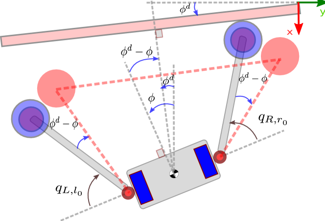
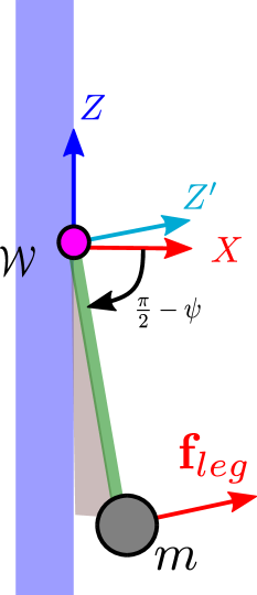
If we chose a $Z-Y-X$ sequence for the Euler angles to represent orientation, the orientation errors about the $Z$ axis can simply be associated with the tracking error in the yaw direction: $\phi^{d}-\phi$. To align the prismatic leg and the landing links to the wall, it suffices to continuously adjust their set-points as follows (see Fig. 11):

$$q^{d}_{L,i} =q_{{L,i}_{0}}+(\phi^{d}-\phi),\quad\quad\quad i\in\{l,r\},$$ (43)

where $\phi$ is the actual value of the yaw angle that can be obtained from the rotation matrix ${}_{w}\mathbf{R}_{b}$, which represents the orientation of the base link:

$$\phi =\arctan({}_{w}\mathbf{R}_{b_{21}},{}_{w}\mathbf{R}_{b_{11}}).$$ (44)

This approach is meant to have good performance in face of orientation errors up to $0.6$ rads. This value is related to the maximum opening of the landing joints, namely, when the landing link is aligned with the base link $Y$ axis.

5.2 Flying motion control: landing

The purpose of the landing mechanism is twofold: 1) to dissipate the excess of kinetic energy at the landing, to avoid bounces and 2) to keep the robot firm on the wall for maintenance operations. During the flight phase, the central thrusting leg is retracted and the landing legs are extruded in order to make contact with the wall during the landing phase. At impact, the kinetic energy

$$\tau^{d}_{L,i} =K_{L}(q^{d}_{L,i}-q_{L,i})-D_{L}\dot{q}_{L,i}\quad\quad\quad i\in\{l,r\},$$ (45)

is dissipated through a joint impedance control law implemented for the $q_{L,l}$ and $q_{L,r}$ joints, with stiffness $K_{l}$ and damping $D_{l}$ selected to achieve a critically damped behaviour. The damping value is set considering the reflected inertia of the robot at the joint level. This control strategy avoids the robot bouncing, thus ensuring a constant contact. For the sake of simplicity, we did not consider the influence of the ropes and gravity force in the impedance law. This is reasonable since, at the impact, the gravity forces and the rope forces are aligned with the landing joint axis; this alleviates their adverse effects on the landing joints (unless the wall is significantly slanted). A more accurate design of a Cartesian impedance controller could be implemented, considering the full (constrained) robot dynamics [39], but this is left for future developments. Notice that, once the joint impedance law takes care of the kinetic energy in the direction perpendicular to the wall, any residual lateral effect can be dissipated with mechanical damping from the landing wheels.

6 Simulation Results

This section presents simulation results to show how the proposed package of solutions enables the robot to navigate along the mountain wall.

6.1 Simulation Setup and Model Validation

We simulate the robot in a Gazebo environment, which computes the full robot (constrained) dynamics using the ODE physic engine [40]. We employ the Unified Robot Description Format (URDF) [41] formalism to describe the robot model and the Pinocchio library [42] to compute the kinematic functions. We always initialise the simulation in a way that the closed loop kinematic constraints are satisfied at the startup (i.e. at a joint configuration $\mathbf{q}_{\text{init}}$).

The optimisation has been implemented in Matlab using the fmincon function. To improve performance, we used a C++ implementation of the Optimal Control Problem (OCP) both for motion planning and control, which is freely available.

As in [22], in a first experiment, we run the optimisation to perform a jump from an initial position $\mathbf{p}_{0}=\begin{bmatrix}0.2&2.5&-6\end{bmatrix}^{T}$ m to a target position $\mathbf{p}_{tg}=\begin{bmatrix}0.2&4&-4\end{bmatrix}^{T}$ m. We validate the results for both the reduced model (in a Matlab environment) and the full model (in Gazebo). For the Matlab simulation, we simply integrate (6) with an ode45 Runge-Kutta variable-step scheme. For the Gazebo simulation, we setup a state machine that orchestrates the 3 phases of the jump: leg orientation, thrusting and flying. The offline optimisation is run before the leg orientation phase, providing the values of the initial impulse ($\mathbf{f}_{\mathrm{leg}}^{*}$), the pattern of the rope forces $\mathbf{F}_{r,l}^{*}$, $\mathbf{F}_{r,r}^{*}$ and the jump duration $t_{f}^{*}$. Since the simulation runs at 1 kHz ($dt_{\text{sim}}$ = 0.001 s) while the optimised trajectory has a different time discretisation ($d_{t}=t_{f}/N$), depending on the jump duration $t_{f}$, appropriate interpolations are performed to adapt the rate difference. During the thrusting phase, we generate the pushing impulse $\mathbf{f}_{\mathrm{leg}}$ at the CoM by applying a force $\mathbf{f}_{c}$ at the contact point.

To avoid generating moments at the CoM, we perform a preliminary step (leg orientation phase) to align the prismatic leg to the direction of $\mathbf{f}_{c}$. To achieve this, we command the set-points for hip roll and hip pitch joints to be $q_{HR}^{d}=\textrm{atan2}(\mathbf{f}_{\mathrm{leg},y},\mathbf{f}_{\mathrm{leg},x})$ and $q_{HP}^{d}=-\pi+\textrm{atan2}(\mathbf{f}_{\mathrm{leg},z},\mathbf{f}_{\mathrm{leg},x})$. Then, we employ the leg dynamics to map the contact force $\mathbf{f}_{c}=\mathbf{f}_{\text{leg}}$ into torques $\bm{\tau}_{\text{leg}}^{d}$ at the leg joints:

$$\bm{\tau}_{\text{leg}}^{d}=\begin{bmatrix}\tau_{HP}\\ \tau_{HR}\\ \tau_{K}\end{bmatrix}=\mathbf{h}_{\text{leg}}(\mathbf{q},\dot{\mathbf{q}})-\mathbf{J}_{c,{\text{leg}}}^{T}(\mathbf{q}){\mathbf{f}}_{c},$$ (46)

where $\mathbf{J}_{c,{\text{leg}}}\in\mathbb{R}^{3\times 3}$ is the sub-matrix of the Jacobian $\mathbf{J}_{c}$, whose columns are relative to the leg joints, and $\mathbf{h}_{\text{leg}}\in\mathbb{R}^{3}$ represents the bias terms (Centrifugal, Coriolis, gravity).

In general, a PD controller is superimposed to the feed-forward torques $\bm{\tau}_{\text{leg}}^{d}$ to drive the leg joints $q_{HR},q_{HP},q_{K}$. However, during the thrusting phase, only the feed-forward torques $\bm{\tau}_{\text{leg}}^{d}$ are applied, while the PD controller is switched off. Finally, during the flying phase, the rope (prismatic) joints are actuated in force control mode. The optimised force patterns $\tau_{RP,l}^{d}=f_{r,l}^{*}$ and $\tau_{RP,r}^{d}=f_{r,r}^{*}$ are set as reference forces for the whole jump duration $t_{f}$. During the flight, the landing mechanism and the prismatic leg are continuously reoriented to be always aligned with the wall face, as explained in Section 5.1.

Figure 12 reports the results in open loop. Simulating the simplified model, the final error norm is below $0.06$ m (due to integration errors), while in the full-model simulation, it is around $0.34$ m. These errors are in a range that can be efficiently handled by a controller, as demonstrated in Section 5. However, the purpose of this validation is to show that the proposed reduced model is a good approximation of the real system and it is sufficient to generate feasible jumps trajectories that do not involve large orientation changes.

Figure 12: Simulation. Open loop validation of the optimisation results. Reference position for the CoM from optimisation (red), simulated trajectory with Matlab (blue) and Gazebo (black).

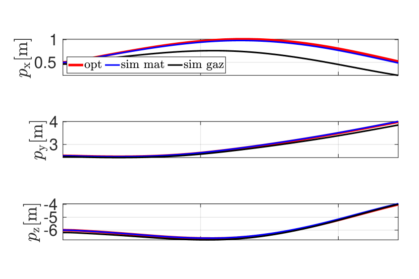
Table 1 reports the value of the physical parameters used in the simulation, together with the optimisation settings, that achieve a good compromise between accuracy and convergence rate.

Table 1: Simulation and optimisation parameters

Name	Symbol	Value
Robot mass [kg]	$m$	5, 13 (with land. mech)
Anchor distance [m]	$d_{a}$	5
Left Anchor position [m]	$\mathbf{p}_{a,l}$	$\begin{bmatrix}0&0&0\end{bmatrix}$
Right Anchor position [m]	$\mathbf{p}_{a,r}$	$\begin{bmatrix}0&b&0\end{bmatrix}$
Friction coeff. []	$\mu$	0.8
Contact normal	$n_{c}$	$\begin{bmatrix}1&0&0\end{bmatrix}$
Wall normal	$n$	$\begin{bmatrix}1&0&0\end{bmatrix}$
Thrust impulse duration [s]	$t_{\text{th}}$	0.05
Discretisation steps (NLP)	$N$	30
Simulation time interval [s]	$dt_{\text{sim}}$	0.001
Sub-integration steps	$N_{\text{sub}}$	5
Hoist work weight	$w_{\text{hw}}$	0.1
Smoothing weight	$w_{s}$	1
Integration method	-	RK4
Max. (normal) leg force [N]	$f_{\mathrm{leg}}^{\text{max}}$	300, 600 (with land. mech)
Max. rope force [N]	$f_{r}^{\text{max}}$	90, 300 (with land. mech)
Jump Clearance [m]	$c$	1
Slack [m]	$s$	0.02
Discretisation steps (MPC)	$N_{\text{mpc}}$	50
Tracking term weight (MPC)	$w_{p,\text{mpc}}$	1
Terminal cost weight (MPC)	$w_{pf,\text{mpc}}$	0
Smoothing weight (MPC)	$w_{u,\text{mpc}}$	$10^{-5}$

Integration errors. To decrease the computational load of the optimisation process, we can reduce the density of the trajectory’s discretisation, which refers to the number of specified points $N$, also known as knots. This reduction, however, results in integration errors, particularly in single shooting settings. First-order integration methods, such as Explicit Euler, may not be sufficient to strike a good balance between computational time and accuracy. To improve accuracy, we found beneficial using higher order integration schemes like Explicit Runge Kutta 4 (RK4) and to perform a number of $N_{\text{sub}}$ integration sub-steps of the dynamics within two adjacent knots. We considered that the rope forces remain constant on the time interval $dt$ between two knots.

In Table 2 we evaluate different combinations of: 1) number $N$ of discretisation nodes, 2) number of sub-steps $N_{\text{sub}}$ and 3) integration method of different order (Euler or RK4). We benchmark on the same experimental jump employed in validation. We report the number of iterations needed to converge, the solution time, the absolute error at the end of the trajectory with respect to the target $\mathbf{e}_{a}=\mathbf{p}_{tg}-\mathbf{p}(t_{f})$, and the error due to integration $\mathbf{e}_{i}=\mathbf{p}_{gt}-\mathbf{p}(t_{f})$, where $\mathbf{p}_{gt}$ is the final position obtained by integrating with a smaller time step of $0.1$ ms.

Table 2: Performances of different integration schemes

$N$	Method	$N_{sub}$	Iters	Comp, Time [$s$]	$\|\mathbf{e}_{i}\|$	$\|\mathbf{e}_{a}\|$
40	RK4	0	44	1.19	0.141	0.148
60	RK4	0	30	1.74	0.045	0.17
40	RK4	5	26	2.1	0.1	0.144
40	EUL	0	28	0.28	0.83	0.85
40	EUL	10	28	1.32	0.05	0.167
30	RK4	5	34	1.71	0.037	0.134

From Table 2 it is evident that both the computation time and the integration error $\|\mathbf{e}_{i}\|$ are linearly proportional (directly and inversely) to the number of discretisation points $N$. Increasing either the number of sub-steps $N_{\text{sub}}$ or the order of integration (i.e. using RK4 instead of Euler) makes the single iteration slower but it makes an accuracy improvement; instead, by reducing $N$, the accuracy decreases. Adding a certain number of integration sub-steps allows to reduce $N$ keeping the accuracy unaltered. Setting $N$ too low the problem can become ill conditioned and convergence might not be achieved. As expected, being RK4 a higher order method, it is superior than Forward Euler in terms of accuracy and requires a lower number of knots $N$ to achieve the same accuracy. As a reasonable trade off, we selected the RK4 with $N=30$ and $N_{\text{sub}}=5$ intermediate integration steps.

6.2 MPC Disturbance tests

To evaluate the effectiveness of the MPC (Section 5) in tracking and rejecting disturbances during the flight phase, we conducted a test similar to the one of the previous section, but with the presence of disturbances. We set $N_{\text{mpc}}=0.4N$ and $dt_{\text{mpc}}$ equal to the optimal control time step $dt$. Since the MPC optimisation takes on average $0.8$ s to be computed, to avoid delays in the simulation, we paused the simulation during the optimisation. We postpone to future work a customised C++ implementation more performing than the C++ code generated from Matlab.

Figure 13 presents the tracking plots for the $3$ reduced states $(\psi,l_{1},l_{2})$ when both an impulsive and a constant disturbance are applied to the robot base. The impulsive disturbance is applied after lift-off and persists for $0.2$ s, while the constant disturbance is applied during the whole jump. This test has the purpose to emulate the effect of wind. The MPC is able to compensate the impulsive disturbance only after $1.4$ s, reaching the target with a cumulative error of $7.2$ cm. The error during the transient in the impulsive case is related to the presence of the unilateral constraint ($f_{r,i}\leq 0$), which is hit by the left rope.

Thanks to the predictive capability of MPC, despite the saturation of the control inputs, the tracking error is reduced.

Figure 13: Simulation with MPC. Tracking of the state variables in face of an impulsive $\bm{\delta}_{i}=[50,-50,30]^{T}$ N (black) and constant disturbance (blue) $\bm{\delta}_{c}=[7,-7,0]^{T}$ N. The last plot shows the rope forces in the case of the impulsive disturbance.

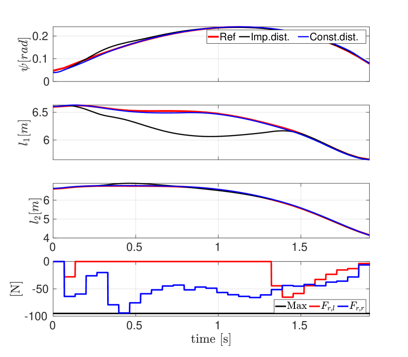
Notably, the impulsive disturbance test reveals that the disturbance it is more promptly rejected on the $\psi$ variable compared to the other states. This can be attributed to the assumption of having bilateral actuation in the propeller thrust forces (i.e. no unilateral constraint). In the case of constant disturbance, the controller proficiently compensated the disturbance at steady state and during the transient, showing a landing error of $7.3$ cm.

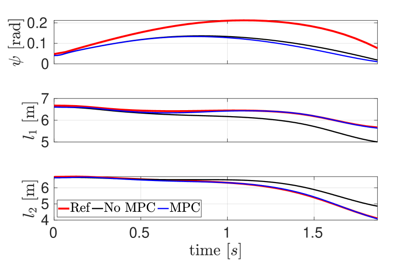
Ablation Study. In this paragraph, we want to evaluate how performance degrades when the propeller is not present (e.g. a propeller is not installed for cutting costs). We repeated the last tests switching off either the propeller or the whole MPC controller. The results are reported both in Fig. 14 and Fig. 15. The plots reveal that the errors are completely recovered (the MPC controller is still active on the ropes) only on $l_{1}$ and $l_{2}$ (with a cumulative error of $6$ cm for $l_{1}$ and $l_{2}$ at landing), while there is a remarkable worsening in the tracking of $\psi$.

Figure 14: Ablation study. Simulation with impulsive disturbance $\bm{\delta}_{i}$ without propellers.

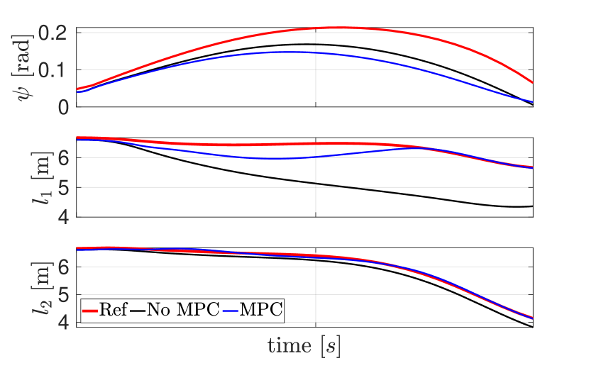
This is related to the fact that the system is under-actuated and the rope forces are constrained on a plane. Therefore, errors on $\psi$ cannot be easily recovered.

Figure 15: Ablation study. Simulation with constant disturbance $\bm{\delta}_{c}$ without propellers.

6.3 Disturbance Rejection: robustness evaluation

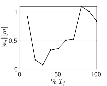
In this section, we test the controller under random impulsive disturbances applied at different moments of the flight phase. We repeat 100 tests with random disturbances with amplitudes between $25$ N and $50$ N. We limit the disturbance to a downward hemisphere 1) to avoid unloading the ropes and 2) because it is more representative of a real situation (e.g. rock-falling from above). To quantitatively evaluate the tracking performance during the flight phase, we completely retract the prismatic leg to avoid early or delayed touch-down and let the simulation stop at the end of the horizon ($t=t_{f}$), where we evaluate the difference between the position of the robot and the desired target. This discrepancy is referred to as the landing error $\mathbf{e}_{a}$. We discretised the flight phase in 10 intervals of equal duration. For each interval we performed 10 tests applying a randomised disturbance in that interval. In Fig. 16 (left) we report $\|{\mathbf{e}}_{a}\|$ as a function of the moment the random disturbance is applied. The plot shows an increasing trend for the error if the impulse is applied close to touchdown, because the controller has no time to compensate it, but similarly its effect is mitigated by the short time to touch-down. As a result, $\|{\mathbf{e}}_{a}\|$ is limited in a small range, which is an indicator of the capability of the controller to reject a variety of constant disturbances in different directions.

Figure 16: (left) Mean of the norm of the landing error $\|{\mathbf{e}}_{a}\|$ for a random impulsive disturbance applied at different moments of the flight phase. The duration of the flight phase is normalized: 0 is lift-off and 100 is touch-down moment. (right) Set of targets to evaluate jumps of variable length and directions. The first target is the rightmost (blue), the others in the list are in CCW order.

Regarding the constant disturbance, we repeated the experiment for the 6 directions that represent the vertices of a cube, with a constant amplitude of 7 N. The norm of the landing error $\|\mathbf{e}_{a}\|$ is reported in Table 3. Except for the $\begin{bmatrix}0&1&0\end{bmatrix}$ direction, they have the same order of magnitude, which is an indicator of the capability of the controller to reject a variety of constant disturbances of different directions. A constant disturbance in direction $\begin{bmatrix}0&1&0\end{bmatrix}$ ($Y$) is problematic for this specific jump because it would require mainly the action of the left rope to be rejected, which is almost unloaded for the landing point $\mathbf{p}_{tg}$.

Table 3: Tracking errors with constant disturbance

Dist. direction	$\|\mathbf{e}_{a}\|$ [$m$]
$\begin{bmatrix}1&0&0\end{bmatrix}$	0.0512
$\begin{bmatrix}-1&0&0\end{bmatrix}$	0.0539
$\begin{bmatrix}0&1&0\end{bmatrix}$	2.4885
$\begin{bmatrix}0&-1&0\end{bmatrix}$	0.2109
$\begin{bmatrix}0&0&1\end{bmatrix}$	0.0835
$\begin{bmatrix}0&0&-1\end{bmatrix}$	0.1384

6.4 Multiple targets: omni-directional jumps

We now aim to demonstrate the effectiveness of the control inputs obtained from the offline optimization process presented in Section 4 in maneuvering the robot to reach various target locations.

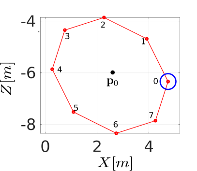
It is important to highlight that while we consider the wall to be vertical, a similar approach has also been proven to work for jumps from non-vertical (i.e. slanted) surfaces [22]. To showcase the capabilities of our approach, we have generated a total of 8 target points, evenly distributed on an ellipse around the $\mathbf{p}_{0}$ location on the wall. The main axis of the ellipse measures $2.5$ m and is inclined at an angle of $45$ degrees with respect to the horizontal plane. The minor axis, on the other hand, spans a length of $2$ m (refer to Fig. 16(right) for a visual representation). This has the purpose to evaluate how good the optimization generalises to different jump lengths and directions. The simulation results are reported in Table 4 and in the accompanying video.

We compute the energy consumption $E$ for each jump, considering the energy consumed in winding/unwinding the ropes and in the pushing impulse:

$$E=\frac{1}{2}m\|\mathbf{\dot{p}}(t_{\text{th}})\|^{2}+\int_{0}^{t_{f}}\left(|f_{r,l}(t)\dot{l}_{1}|+|f_{r,r}(t)\dot{l}_{2}|\right)dt,$$ (47)

where the former is proportional to the kinetic energy of the robot evaluated at the lift-off ($t=t_{\text{th}}$) (assuming the robot starting standstill). The second term is the energy consumed by the hoist motors as the integral of the power along the whole jump duration $t_{f}$. The hoist work, in general, dominates. In a first batch of tests we set the weight relative to the hoist work $w_{hw}=0$ in (41). In another set of experiments we set a non zero weight for the hoist work $w_{hr}=100$.

To demonstrate the robustness of the approach in a real application where states derivatives are usually obtained by numeric differentiation of encoder readings, we added a zero-mean white Gaussian noise to the state with standard deviation $\bm{\sigma}=\begin{bmatrix}0.01\,\mbox{rad/s}&0.2\,\mbox{m/s}&0.2\,\mbox{m/s}\end{bmatrix}$.

Table 4 reports mean and standard deviation of the norm of the absolute landing error $\mathbf{e}_{a}=\mathbf{p}_{tg}-\mathbf{p}(t_{f})$ and the energy consumption $E$ for each jump. To better appreciate the impact of noise we also report between parenthesis the values without noise.

Table 4: Tracking error and energy consumption without hoist work penalization

Exp.	$\mathbf{p}_{tg}$ [m]	$\|\mathbf{e}_{a}\|$ [m]	$E$ [J]
0	$\begin{bmatrix}0.28&4.73&-6.34\end{bmatrix}$	(0.6) 0.9 $\pm$ 0.19	(103) 162 $\pm$ 111
1	$\begin{bmatrix}0.28&3.91&-4.69\end{bmatrix}$	(0.078) 0.3 $\pm$ 0.008	(119) 129 $\pm$ 4
2	$\begin{bmatrix}0.28&2.26&-3.86\end{bmatrix}$	(0.079) 0.4084 $\pm$ 0.16	(200) 147 $\pm$ 16
3	$\begin{bmatrix}0.28&0.75&-4.35\end{bmatrix}$	(0.081) 1.5 $\pm$ 0.95	(287) 607 $\pm$ 317
4	$\begin{bmatrix}0.28&0.26&-5.86\end{bmatrix}$	(0.066) 0.17 $\pm$ 0.007	(228) 199 $\pm$ 5
5	$\begin{bmatrix}0.28&1.08&-7.51\end{bmatrix}$	(0.067) 0.24 $\pm$ 0.06	(261) 214 $\pm$ 45
6	$\begin{bmatrix}0.28&2.73&-8.34\end{bmatrix}$	(0.08) 0.2653 $\pm$ 0.044	(32) 202 $\pm$ 71
7	$\begin{bmatrix}0.28&4.25&-7.85\end{bmatrix}$	(0.32) 0.62 $\pm$ 0.27	(78) 152 $\pm$ 108

Interestingly, the highest errors are with test 0 and 7, which are the targets that are closer to the vertical of the right anchor (i.e. at $\mathbf{p}_{{a,r}_{y}}=5$ m). This is reasonable because in these tests one of the two ropes is almost unloaded and cannot control properly the error in the $Y$ direction. This suggests that a reduction in performance occurs when one of the ropes is almost unloaded. For the other tests, the error is on average around $0.07$ m. The noise results in higher errors with a similar trend, except for test 3, which resulted in a significantly higher average error of $2.22$ m. Inspecting the collected data for that target, we noted that the error had an erratic behaviour being very high only in some tests that increase the overall mean, while others are in the same range as 1, 2, 4, 5, 6. We conjecture that this is related to the fact that test 3, being an upward jump, was exceptionally demanding for the left rope that was working at the boundary of its physical actuation limits.

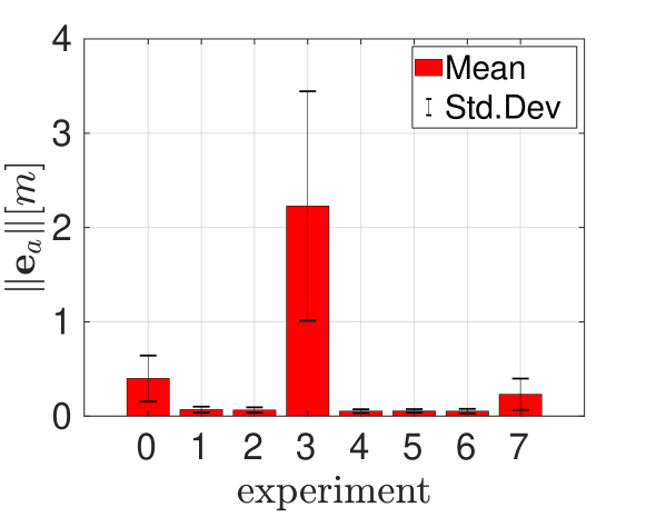
Regarding the consumed energy, this is low for jumps to a lower point (i.e. 6, 7), because the gravity helps and the ropes can be let to passively unwind the ropes to attain the target. However, it was surprisingly high for tests 3, 4, and 5. The reason is that, because there was no penalization in the cost function, the optimiser found elaborated trajectories to reach the target with high accuracy disregarding the energy. Therefore, we repeated the previous tests penalising, this time, the hoist work. The results are reported in Table 5.

Table 5: Tracking error and energy consumption with hoist work penalization

Exp.	$\mathbf{p}_{tg}$ [m]	$\|\mathbf{e}_{a}\|$ [m]	$E$ [J]
0	$\begin{bmatrix}0.28&4.73&-6.34\end{bmatrix}$	(0.4) 0.4 $\pm$ 0.244	(19.4) 152 $\pm$ 125
1	$\begin{bmatrix}0.28&3.91&-4.69\end{bmatrix}$	(0.067) 0.068 $\pm$ 0.0315	(54 ) 120 $\pm$ 4
2	$\begin{bmatrix}0.28&2.26&-3.86\end{bmatrix}$	(0.071) 0.064 $\pm$ 0.278	(124) 171$\pm$ 42
3	$\begin{bmatrix}0.28&0.75&-4.35\end{bmatrix}$	(0.077) 2.22 $\pm$ 1.21	( 97) 568 $\pm$ 210
4	$\begin{bmatrix}0.28&0.26&-5.86\end{bmatrix}$	(0.07) 0.06 $\pm$ 0.023	(45 ) 200 $\pm$ 11
5	$\begin{bmatrix}0.28&1.08&-7.51\end{bmatrix}$	(0.095) 0.06 $\pm$ 0.018	(14 ) 224 $\pm$ 54
6	$\begin{bmatrix}0.28&2.73&-8.34\end{bmatrix}$	(0.12) 0.053 $\pm$ 0.024	(10 )236$\pm$ 75
7	$\begin{bmatrix}0.28&4.25&-7.85\end{bmatrix}$	(0.28) 0.23 $\pm$ 0.16	(13 ) 160 $\pm$ 117

In this case, the optimiser managed to find solutions that are more energy efficient, with similar accuracy. The trend is now inline with the physical intuition that targets above $\mathbf{p}_{0}$ (i.e. 1, 2, 3) are more energy demanding than the ones below (i.e. 5, 6, 7). The impact of noise (c.f. Fig. 17) is similar to the previous case.

Figure 17: Mean and standard deviation for 50 repetitions of each test in Fig. 16 (with hoist work penalisation) adding white Gaussian Noise to the state derivatives.

To highlight the versatility of the approach, in the accompanying video, we conducted additional tests by placing the anchor points at different locations, specifically 5, 7, 9, and 11 meters apart. Despite these varying placements, our optimization algorithm still successfully produces valid results. We observed that the proposed method yields different solutions for the same target based on the anchor location, yet in all cases a level of landing accuracy comparable with the previous experiments is achieved.

6.5 Obstacle avoidance

In this section we test capability of the optimal planner to deal with a non-flat wall surface. We model an obstacle as a hemi-ellipsoid whose semi axes are $R_{x}=1.5$ m, $R_{y}=1.5$ m and $R_{z}=0.87$ m, with centre $\mathbf{o}=\begin{bmatrix}-0.5&2.5&-6\end{bmatrix}^{T}$ m. To implement obstacle avoidance we set a path constraint $f(\mathbf{x})>0$ on the $X$ component of the robot position: $\mathbf{p}_{x}>\hat{x}+c$. Where $c$ is a clearance margin that should be kept from the obstacle, for safety. $\hat{x}\in\mathbb{R}$ is a function $f(\mathbf{p}_{y},\mathbf{p}_{z})$ that can be easily obtained from the ellipsoid equation:

$$\begin{aligned} &\hat{x}=\mathbf{o}_{x}+\sqrt{q},\\ &q=R_{x}^{2}-\frac{R_{x}}{R_{y}}(\mathbf{p}_{y}-\mathbf{o}_{y})-\frac{R_{x}}{R_{z}}(\mathbf{p}_{z}-\mathbf{o}_{z})^{2}.\\ \end{aligned}$$ (48)

To ensure that the constraint is enforced only for positions in the convex hull of the ellipsoid (where the square root is defined), we check if the argument $q$ of the square root is positive, otherwise we consider the usual wall constraint (34):

$$\begin{cases}\mathbf{p}_{x}>\hat{x}+c,\quad&q>0,\\ \mathbf{p}_{x}>\epsilon,\quad&q<0.\end{cases}$$ (49)

Considering this constraint, and setting a clearance $c=1$ m, we optimize a jump starting from a point $\mathbf{p}_{0}=\begin{bmatrix}0.5&0.5&-6\end{bmatrix}^{T}$ (to the left of the obstacle) to reach a target $\mathbf{p}_{tg}=\begin{bmatrix}0.5&4.5&-6\end{bmatrix}^{T}$ (to the right). The accompanying video shows that the optimisation is able to find a trajectory that allows the robot to successfully overpass the obstacle. One limitation of the actual approach, is that targets that are in the shade cone of the obstacle, could not be reached. This is because the ropes would collide with the obstacle, unless the obstacle is small enough and the ropes come from the sides. Another limitation is that the optimisation turned out to be very sensitive to the relative location of obstacle and target and required fine parameter tuning to achieve convergence.

6.6 Landing test

In this section, we conduct a simulation of the robot equipped with the landing mechanism presented in Section 2.1.1 with the aim of assessing the effectiveness of the landing strategy in dissipating any excess kinetic energy during touchdown without causing any rebound with the additional difficulty of a slanted wall, as discussed below.

Depending on the accumulated errors during the flight phase, the touch-down could be either early or delayed with respect to the duration of the optimised trajectory. In the case that the touch-down is delayed, we use the feed-forward coming from the optimisation to determine the ropes forces and we apply a gravity compensation action. Due to the additional weight of the lander, in these tests, we increased the mass to $15$ kg. This requires that we also ought to adjust the actuation limits: $f_{\mathrm{leg},\max}=600$ N and $f_{r,\max}=300$ N. The landing joints $q_{L,f}$ are controlled through the PD strategy (45) with stiffness and damping set to $K_{L}=60$ N/m and $D_{L}=10$ N/m respectively.

Figure 18 reports the tracking of the Cartesian position of the robot for the landing test. It is evident, inspecting the first plot ($X$ variable), that the robot is able to land without re-bounce and that an early touch-down occurred.

Figure 18: Simulation of the landing test for a wall inclination of 0.1 rad from the vertical. The red and blue plots are the reference and actual position of the robot, respectively. The vertical red shaded line highlights the early touch-down moment.

7 Conclusions

This paper presents a robotic platform designed to execute rescue and maintenance operations along mountain slopes. The robot hangs on two ropes that are attached to anchors deployed on the top of the wall. The motion is guaranteed by two motors that wind and un-wind the ropes, and by a retractable leg that pushes away the robot from the mountain. An auxiliary propeller guarantee the stability of the robot during the flight phases. We have discussed in depth the design of the robot, and shown a simplified dynamic model that captures the dominant components of the system’s dynamics, while being mathematically tractable. The model has been used to design motion planning and control strategies based on a suitable MPC formulation. The paper also discusses effective means to compute the locations where the system can be in equilibrium and apply sufficient forces on the wall (e.g., to scale boulders, or drill holes). As an essential part of our work, we also developed a complete and realistic simulation model that we used to collect a large number of simulation results in different application scenarios.

This paper could open the way to a large amount of future work, addressing the problems that this novel platform and its potential applications have unveiled. A non-complete list includes: 1. developing a multi-jump motion planner that considers the hybrid dynamics of the system to plan the system actions across the mode transitions related to the landing-take-off phase; 2. considering a more complete simplified model that accounts for rotational dynamics to improve the control algorithm during the flight phase; 3. developing control strategies for specific operations (e.g., drilling scaling); 4. developing learning approaches to enable jumps on crumbly terrain with hardly predictable responses.

Appendix

Definitions of $\mathbf{A}_{d}$, $\mathbf{b}_{d}$ introduced in  (6) of the reduced order model.

$$\mathbf{A}_{d}=\begin{bmatrix}-\mathbf{p}_{z}&\frac{\mathbf{p}_{x}}{l_{1}}-\frac{\sin(\psi)^{2}\mathbf{p}_{y}}{2d_{a}\mathbf{p}_{x}l_{1}}\left(2l_{1}^{2}-d_{a}\right)&\frac{l_{2}\mathbf{p}_{y}\sin(\psi)^{2}}{d_{a}\mathbf{p}_{x}}\\ 0&\frac{l_{1}}{d_{a}}&-\frac{l_{2}}{d_{a}}\\ \mathbf{p}_{x}&\frac{\cos(\psi)sin(\psi)\mathbf{p}_{y}}{2\mathbf{p}_{x}l_{1}d_{a}}\left(2l_{1}^{2}-d_{a}\right)+\frac{\mathbf{p}_{z}}{l_{1}}&-\frac{l_{2}\mathbf{p}_{y}\cos(\psi)\sin(\psi)}{d_{a}\mathbf{p}_{x}}\end{bmatrix}$$ (50)

$$\mathbf{b}_{d}=\begin{bmatrix}q_{1}-\frac{\sin(\psi)^{2}q_{2}}{q_{4}}-\frac{{\mathbf{p}_{y}2d_{a}}^{2}\sin(\psi)q_{1}^{2}}{q_{3}}+\frac{\dot{\psi}\mathbf{p}_{y}2d_{a}\cos(\psi)q_{1}}{q_{6}}+\frac{\dot{l_{1}}\mathbf{p}_{y}2d_{a}\sin(\psi)q_{1}}{q_{6}l_{1}}\\ \frac{-{\dot{l_{2}}}^{2}+{\dot{l}_{1}}^{2}}{d_{a}}\\ q_{7}+\frac{\cos(\psi)q_{2}}{q_{4}}+\frac{{\mathbf{p}_{y}2d_{a}}^{2}\cos(\psi)q_{1}^{2}}{q_{3}}-\frac{\dot{l}_{1}\mathbf{p}_{y}2d_{a}\cos(\psi)q_{1}}{q_{6}l_{1}}+\frac{\dot{\psi}\mathbf{p}_{y}2d_{a}\sin(\psi)q_{1}}{q_{6}}\end{bmatrix}^{T}$$ (51)

with:

$$\begin{cases}q_{0}=&2\dot{l}_{1}\frac{\mathbf{p}_{z}}{l1}\dot{\psi}-l_{1}{\dot{\psi}}^{2}\frac{\mathbf{p}_{x}}{l_{1}}\\ q_{1}=&-l_{2}^{2}\dot{l_{1}}+2l_{1}l_{2}\dot{l_{2}}-l_{1}^{2}\dot{l_{1}}+d_{a}^{2}\dot{l_{1}}\\ q_{2}=&3{\dot{l}_{1}}^{2}{\mathbf{p}_{y}2d_{a}}^{2}+8l_{1}l_{2}\dot{l}_{1}\dot{l_{2}}\mathbf{p}_{y}2d_{a}-2{l_{1}}^{2}{\dot{l_{2}}}^{2}\mathbf{p}_{y}2d_{a}+4\,{l_{1}}^{2}\,{l_{2}}^{2}\,{\dot{l_{2}}}^{2}\\ &-6\,{l_{1}}^{2}\,{\dot{l}_{1}}^{2}\,\mathbf{p}_{y}2d_{a}-8\,{l_{1}}^{3}\,l_{2}\,\dot{l}_{1}\,\dot{l_{2}}+4\,{l_{1}}^{4}\,{\dot{l}_{1}}^{2}\\ q_{3}=&\frac{16d_{a}^{4}{l_{1}}^{2}{\mathbf{p}_{x}}^{3}}{\sin(\psi)^{3}}\\ q_{4}=&\frac{4d_{a}^{2}{l_{1}}^{2}\mathbf{p}_{x}}{\sin(\psi)}\\ q_{6}=&\frac{2d_{a}^{2}l_{1}\mathbf{p}_{x}}{\sin(\psi)}\\ q_{7}=&-\mathbf{p}_{z}\dot{\psi}^{2}+2\dot{l_{1}}\dot{\psi}\frac{\mathbf{p}_{x}}{l_{1}}\end{cases}$$

References

- Nishi et al. [1986] A. Nishi, Y. Wakasugi, K. Watanabe, Design of a robot capable of moving on a vertical wall, Adv. Robot. 1 (1986) 35–45. doi:10.1163/156855386X00300.
- Potenza et al. [2020] F. Potenza, C. Rinaldi, E. Ottaviano, V. Gattulli, A robotics and computer-aided procedure for defect evaluation in bridge inspection, Journal of Civil Structural Health Monitoring 10 (2020) 471–484.
- Seo et al. [2018] J. Seo, L. Duque, J. Wacker, Drone-enabled bridge inspection methodology and application, Automation in Construction 94 (2018) 112–126.
- Ji et al. [2018] A. Ji, Z. Zhao, P. Manoonpong, W. Wang, G. Chen, Z. Dai, A bio-inspired climbing robot with flexible pads and claws, Journal of Bionic Engineering 15 (2018) 368–378.
- Kim et al. [2008] S. Kim, M. Spenko, S. Trujillo, B. Heyneman, D. Santos, M. R. Cutkoskly, Smooth vertical surface climbing with directional adhesion, IEEE Transactions on Robotics 24 (2008) 65–74. doi:10.1109/TRO.2007.909786.
- Pope et al. [2017] M. T. Pope, C. W. Kimes, H. Jiang, E. W. Hawkes, M. A. Estrada, C. F. Kerst, W. R. Roderick, A. K. Han, D. L. Christensen, M. R. Cutkosky, A Multimodal Robot for Perching and Climbing on Vertical Outdoor Surfaces, IEEE Trans. Robot. 33 (2017) 38–48. doi:10.1109/TRO.2016.2623346.
- Myeong et al. [2015] W. C. Myeong, K. Y. Jung, S. W. Jung, Y. H. Jung, H. Myung, Drone-type wall-climbing robot platform for structural health monitoring, Int. Conf. Adv. Exp. Struct. Eng. 2015-Augus (2015) 1–6.
- Sukvichai et al. [2017] K. Sukvichai, P. Maolanon, K. Songkrasin, Design of a double-propellers wall-climbing robot, in: 2017 IEEE International Conference on Robotics and Biomimetics (ROBIO), 2017, pp. 239–245. doi:10.1109/ROBIO.2017.8324424.
- Alkalla et al. [2017] M. Alkalla, M. Fanni, A. Mohamed, S. Hashimoto, Tele-operated propeller-type climbing robot for inspection of petrochemical vessels, Industrial Robot: An International Journal 44 (2017) 166–177. doi:10.1108/IR-07-2016-0182.
- Yang et al. [2023] L. Yang, B. Li, J. Feng, G. Yang, Y. Chang, B. Jiang, J. Xiao, Automated wall-climbing robot for concrete construction inspection, Journal of Field Robotics 40 (2023) 110–129. URL: https://onlinelibrary.wiley.com/doi/abs/10.1002/rob.22119. doi:https://doi.org/10.1002/rob.22119.
- Nishimura et al. [2022] Y. Nishimura, S. Takahashi, H. Mochiyama, T. Yamaguchi, Automated hammering inspection system with multi-copter type mobile robot for concrete structures, IEEE Robotics and Automation Letters 7 (2022) 9993–10000. doi:10.1109/LRA.2022.3191246.
- Qian et al. [2018] S. Qian, B. Zi, W.-W. Shang, Q.-S. Xu, A review on cable-driven parallel robots, Chinese Journal of Mechanical Engineering 31 (2018) 1–11.
- Korayem et al. [2014] M. Korayem, H. Tourajizadeh, A. Zehfroosh, A. Korayem, Optimal path planning of a cable-suspended robot with moving boundary using optimal feedback linearization approach, Nonlinear Dynamics 78 (2014) 1515–1543.
- Zhang et al. [2018] N. Zhang, W. Shang, S. Cong, Dynamic trajectory planning for a spatial 3-dof cable-suspended parallel robot, Mechanism and Machine Theory 122 (2018) 177–196.
- Newdick et al. [2023] S. Newdick, N. Ongole, T. G. Chen, E. Schmerling, M. R. Cutkosky, M. Pavone, Motion planning for a climbing robot with stochastic grasps, in: 2023 IEEE International Conference on Robotics and Automation (ICRA), 2023, pp. 11838–11844. doi:10.1109/ICRA48891.2023.10160218.
- Lahouar et al. [2009] S. Lahouar, E. Ottaviano, S. Zeghoul, L. Romdhane, M. Ceccarelli, Collision free path-planning for cable-driven parallel robots, Robotics and Autonomous Systems 57 (2009) 1083–1093.
- Polzin et al. [2023] M. Polzin, F. Centamori, J. Hughes, Heading for the abyss: Control strategies for exploiting swinging of a descending tethered aerial robot, in: 2023 IEEE International Conference on Robotics and Automation (ICRA), 2023, pp. 5373–5378. doi:10.1109/ICRA48891.2023.10160347.
- Webpage [2024a] Webpage, Youbube - Blade BUG: the robot that can repair wind turbines, Accessed on 02/2024a. URL: https://www.youtube.com/watch?v=I3X6YlF4jAI.
- Webpage [2024b] Webpage, Youbube - Wind Turbine Blade Repairs - Robotics Revolutionizing the Wind Industry, Accessed on 02/2024b. URL: https://www.youtube.com/watch?v=pz9Wn2Kcj4A.
- Webpage [2024c] Webpage, Rope robotics, Accessed on 02/2024c. URL: https://roperobotics.com/.
- Wang et al. [2014] L. Wang, U. Culha, F. Iida, A dragline-forming mobile robot inspired by spiders, Bioinspiration and Biomimetics 9 (2014). doi:10.1088/1748-3182/9/1/016006.
- Focchi et al. [2023] M. Focchi, M. Bensaadallah, M. Frego, A. Peer, D. Fontanelli, A. Del Prete, L. Palopoli, CLIO: a Novel Robotic Solution for Exploration and Rescue Missions in Hostile Mountain Environments, in: 2023 IEEE International Conference on Robotics and Automation (ICRA), 2023, pp. 7742–7748. doi:10.1109/ICRA48891.2023.10160440.
- Riskin and Racey [2010] D. K. Riskin, P. A. Racey, How do sucker-footed bats hold on, and why do they roost head-up?, Biological Journal of the Linnean Society 99 (2010) 233–240. URL: https://doi.org/10.1111/j.1095-8312.2009.01362.x. doi:10.1111/j.1095-8312.2009.01362.x.
- Bando et al. [2017] M. Bando, M. Murooka, T. Yanokura, S. Nozawa, K. Okada, M. Inaba, Rappelling by a humanoid robot based on transition motion generation and reliable rope manipulation, IEEE-RAS Int. Conf. Humanoid Robot. (2017) 129–135. doi:10.1109/HUMANOIDS.2017.8239547.
- Bando et al. [2018] M. Bando, M. Murooka, S. Nozawa, K. Okada, M. Inaba, Walking on a Steep Slope Using a Rope by a Life-Size Humanoid Robot, IEEE Int. Conf. Intell. Robot. Syst. (2018) 705–712. doi:10.1109/IROS.2018.8594292.
- Hoffman et al. [2021] E. M. Hoffman, M. P. Polverini, A. Laurenzi, N. G. Tsagarakis, Modeling and Optimal Control for Rope-Assisted Rappelling Maneuvers, Proc. - IEEE Int. Conf. Robot. Autom. 2021-May (2021) 9826–9832. doi:10.1109/ICRA48506.2021.9560802.
- Coelho et al. [2021] A. Coelho, Y. S. Sarkisov, J. Lee, R. Balachandran, A. Franchi, K. Kondak, C. Ott, Hierarchical control of redundant aerial manipulators with enhanced field of view, in: 2021 International Conference on Unmanned Aircraft Systems (ICUAS), 2021, pp. 994–1002. doi:10.1109/ICUAS51884.2021.9476739.
- Haldane et al. [2017] D. W. Haldane, J. K. Yim, R. S. Fearing, Repetitive extreme-acceleration (14-g) spatial jumping with salto-1p, IEEE International Conference on Intelligent Robots and Systems 2017-Septe (2017) 3345–3351. doi:10.1109/IROS.2017.8206172.
- Nguyen et al. [2019] Q. Nguyen, M. J. Powell, B. Katz, J. D. Carlo, S. Kim, Optimized jumping on the MIT cheetah 3 robot, Proc. - IEEE Int. Conf. Robot. Autom. 2019-May (2019) 7448–7454. doi:10.1109/ICRA.2019.8794449.
- Chignoli and Kim [2021] M. Chignoli, S. Kim, Online trajectory optimization for dynamic aerial motions of a quadruped robot, in: 2021 IEEE International Conference on Robotics and Automation (ICRA), 2021, pp. 7693–7699. doi:10.1109/ICRA48506.2021.9560855.
- Ding et al. [2021] Y. Ding, M. Zhang, C. Li, H.-W. Park, K. Hauser, Hybrid sampling/optimization-based planning for agile jumping robots on challenging terrains, in: 2021 IEEE International Conference on Robotics and Automation (ICRA), 2021, pp. 2839–2845. doi:10.1109/ICRA48506.2021.9561939.
- Jiang et al. [2022] X. Jiang, W. Chi, Y. Zheng, S. Zhang, Y. Ling, J. Xu, Z. Zhang, Locomotion generation for quadruped robots on challenging terrains via quadratic programming, Auton. Robots (2022). URL: https://doi.org/10.1007/s10514-022-10068-3. doi:10.1007/s10514-022-10068-3.
- Grandia et al. [2022] R. Grandia, F. Jenelten, S. Yang, F. Farshidian, M. Hutter, Perceptive Locomotion through Nonlinear Model Predictive Control, arXiv (2022) 1–20. URL: http://arxiv.org/abs/2208.08373. arXiv:2208.08373.
- Ding et al. [2020] Y. Ding, C. Li, H. W. Park, Kinodynamic motion planning for multi-legged robot jumping via mixed-integer convex program, IEEE Int. Conf. Intell. Robot. Syst. (2020) 3998–4005. doi:10.1109/IROS45743.2020.9341572. arXiv:2011.01809.
- Orsolino et al. [2018] R. Orsolino, M. Focchi, C. Mastalli, H. Dai, G. D. Caldwell, C. Semini, Application of wrench based feasibility analysis to the online trajectory optimization of legged robots, IEEE Robotics and Automation Letters (2018). doi:10.1109/LRA.2018.2836441.
- Delos and Teissandier [2015] V. Delos, D. Teissandier, Minkowski sum of polytopes defined by their vertices, Journal of Applied Mathematics and Physics (2015).
- Dai and Tedrake [2016] H. Dai, R. Tedrake, Planning robust walking motion on uneven terrain via convex optimization, in: 2016 IEEE-RAS 16th International Conference on Humanoid Robots (Humanoids), 2016, pp. 579–586. doi:10.1109/HUMANOIDS.2016.7803333.
- Fukuda and Prodon [1996] K. Fukuda, A. Prodon, Double description method revisited, in: M. Deza, R. Euler, I. Manoussakis (Eds.), Combinatorics and Computer Science, Springer Berlin Heidelberg, Berlin, Heidelberg, 1996, pp. 91–111.
- Mingo et al. [2022] E. Mingo, S. Kothakota, A. Moreno, A. Curti, N. Miguel, L. Marchionni, Whole-body kinematics modeling in presence of closed-linkages: application to the kangaroo biped robot, HAL archive, Id: hal-03652472 https://hal.science/hal-03652472/document (2022).
- Smith [2024] R. Smith, ODE: Open Dynamics Engine, Accessed on 02/2024. URL: https://www.ode.org.
- Webpage [2024] Webpage, URDF Package Summary, Accessed on 02/2024. URL: http://wiki.ros.org/urdf.
- Carpentier et al. [2019] J. Carpentier, G. Saurel, G. Buondonno, J. Mirabel, F. Lamiraux, O. Stasse, N. Mansard, The Pinocchio C++ library – A fast and flexible implementation of rigid body dynamics algorithms and their analytical derivatives, in: IEEE International Symposium on System Integrations (SII), 2019.
Appendix
Definitions of , introduced in (6) of the reduced order model.