Geometric Generative Models based on Morphological Equivariant PDEs and GANs

Abstract

Content and image generation consist in creating or generating data from noisy information by extracting specific features such as texture, edges, and other thin image structures. We are interested here in generative models, and two main problems are addressed. Firstly, the improvements of specific feature extraction while accounting at multiscale levels intrinsic geometric features; and secondly, the equivariance of the network to reduce its complexity and provide a geometric interpretability. To proceed, we propose a geometric generative model based on an equivariant partial differential equation (PDE) for group convolution neural networks (G-CNNs), so called PDE-G-CNNs, built on morphology operators and generative adversarial networks (GANs). Equivariant morphological PDE layers are composed of multiscale dilations and erosions formulated in Riemannian manifolds, while group symmetries are defined on a Lie group. We take advantage of the Lie group structure to properly integrate the equivariance in layers, and are able to use the Riemannian metric to solve the multiscale morphological operations. Each point of the Lie group is associated with a unique point in the manifold, which helps us derive a metric on the Riemannian manifold from a tensor field invariant under the Lie group so that the induced metric has the same symmetries. The proposed geometric morphological GAN (GM-GAN) is obtained by using the proposed morphological equivariant convolutions in PDE-G-CNNs to bring nonlinearity in classical CNNs. GM-GAN is evaluated on MNIST data and compared with GANs. Preliminary results show that GM-GAN model outperforms classical GAN.

Keywords: Partial differential equations. Equivariance. Morphological operators. Riemannian manifolds. Lie group. Symmetries. Convolution neural networks.

1 Introduction

Content generation is one of the most quickly developing domain, mainly because of its potential real life applications. Encouraging results of generative models are due to prominent advances in learning methods based on adversarial neural network. Generative models outperform CNNs in many aspects; for instance, samples outside the training set can be created or rejected by generative models, while CNNs and recursive NNs fail to do so. This capability to generate data beyond mere density estimation makes generative models become very important for the prediction of samples outside the training set, and may be a reason of their high interests in recent years. Generative models also have found many interesting real life applications in various domains; for instance, in realistic synthetic images generation, content generation from words and phrases [54, 71], adversarial training [55], missing data completion [68, 43, 70], image manipulation based on predefined features [37, 53, 18, 50, 45, 72], multimodal tasks with a single input [42, 63], samples generation from the same distribution [3, 66], data quality enhancement [48, 57, 67]. GANs [40, 39] brought a new perspective to the deep learning community, deep learning with adversarial training is considered today as one of the most robust technique. With adversarial generative networks, there exists not only a good neural network-based classifier, referred to as the discriminator network, but also a generative network capable of producing realistic adversarial samples, all within a single architecture. This means that we now have a network that is aware of internal representations through its training to distinguish real inputs from artificial ones. Many extensions have been built for increasing its performances. Conditional GAN (CGAN) [37] was proposed as an extension of original GAN for generating facial images on the basis of facial attributes. Deep Convolutional GAN (DCGAN) [53] was proposed for image generation where both the generator and discriminator networks are convolutional. GRAN [44] is a GAN model based on a sequential process. Bidirectional GAN (BiGAN) and extensions [27, 17] were proposed to map data into a latent code similar to an autoencoder. Generative Multi-Adversarial Network (GMAN) [32] was proposed for extending the minimax game to multiple players in GANs. In a different perspective, Wasserstein Generative Adversarial Network (WGAN) [4] was introduced as one of the most distinguished GAN models, because it reduced instability issues during the training and removed the effect of mode collapse. GANs and variants lack an inference mechanism.

Related works

Significant advances in deep learning progress are attributed to CNNs [41]. Despite its successful applications in many real life problems, it is still not very clear why deep learning techniques work. Pursuing this goal, many works attempt to give an answer to this so challenging question by setting mathematical frameworks that underlie the process. A promising direction is to consider symmetries as a fundamental design principle for network architectures. This can be implemented by constructing deep neural networks that are compatible with a symmetry group that acts transitively on the input data. Among noticeable properties in CNNs, the equivariance concerning translations played an important role. Equivariance means that the operation of performing a transformation of the input data then passing them through the network is the same as passing the input data through the network and then performing a transformation of the output. Deep neural networks are inherently translationally invariant; however, invariance does not extend straightforward to other types of transformations. G-CNNs [21, 12, 23] were introduced to tackle this issue by generalizing CNNs in a way such that symmetries are incorporated and fully exploited in the learning process. In addition to reducing a lot sample complexity by exploiting symmetries since there is no more need to learn them, G-CNNs show great improvements compared to former CNNs [65, 22, 11]. Very recently, PDE-G-CNNs [60, 13] were proposed as PDEs-based framework based that generalized G-CNNs. Authors proposed to replace the classical convolution, pooling and ReLUs in traditional CNNs by resolving a PDE composed of four terms where each one behaved separately like a convection, diffusion, dilation and erosion. The proposed PDEs were solved by providing analytical kernels approximations [60] and exact kernels sub-Riemannian approximations [13]. PDE-G-CNNs were shown to increase the performance for classification tasks. Intensive research on equivariant operators other than transformations is still conducted [56, 38, 62].

Paper contributions

Main contributions are: 1) improving of specific feature extraction while accounting at multiscale levels intrinsic geometric features, and 2) making the network equivariant for reducing its complexity and providing a geometric interpretability. As for alternatives for these issues, 3) we propose here a new geometric generative model based on a new PDE-G-CNNs built on multiscale morphology operators and geometric image processing techniques.

Manuscript organization

In Section 2, we recall some background on multiscale mathematical operators and their links with PDEs. In Section 3, we define the notion of equivariance in Lie groups and present the group invariance property on Riemannian manifolds. In Section 4, we present the viscosity solutions for morphological dilations and erosions formulated as Lie group morphological convolutions in Riemannian manifolds. The proposed geometric generative (GM-GAN) model in presented in Section 5. Section 6 is dedicated to numerical experiments and comparisons with classical GAN models. The paper ends in Section 7 where concluding remarks and perspectives are discussed.

2 Background on PDEs-based mathematical morphology

Let $b:\mathds{R}^{2}\rightarrow\bar{}\mathds{R}$ be a concave function, known also as the structuring function or convolution kernel. Let us consider the subset $\mathds{E}$ of $\mathds{Z}^{2}$ and the function $f:\mathds{E}\rightarrow\bar{}\mathds{R}$.

Definition 2.1

Morphological dilation and erosion are respectively defined as:

$$f\oplus b(x)=\sup_{y\in\mathds{E}}[f(y)+b(x-y)]$$ (1)

$$f\ominus b(x)=\inf_{y\in\mathds{E}}[f(y)-b(y-x)].$$ (2)

Let $B\subseteq\mathds{E}$ be a bounded set. A flat structuring function (SF) satisfies $b(x)=0$ if $x\in B$ and $b(x)=-\infty$ if $x\in B^{c}$. The flat morphological dilation and erosion respectively write:

$$f\oplus B(x)=\sup_{y\in B}[f(x-y)]\mbox{ and }f\ominus B(x)=\inf_{y\in B}[f(x+y)].$$ (3)

As for an interpretation, erosion shrinks positive peaks, and peaks thinner than the structuring function disappear. One has the dual effects for morphological flat dilation. Both the morphological dilation and erosion are translation invariant.

Definition 2.2

Let $\mathcal{F}$ be a family of real functions defined on $\Omega\subseteq\mathds{R}^{2}$. We say that $T:\mathcal{F}\rightarrow\mathcal{F}$ is said to be increasing (monotone) if and only if it satisfies:
$\forall~{}f_{1},f_{2}\in\mathcal{F}$ such that $(f_{1}\geq f_{2}$ on $\Omega)$ implies $(T(f_{1})\geq T(f_{2})$ on $\Omega)$.

Proposition 2.1

Morphological dilation and erosion satisfy the following duality and adjunction properties:

1. duality: $f\oplus b=-(-f\ominus b)$

2. adjunction: $(f_{1}\oplus b\leq f_{2}$ on $E)$ $\Longleftrightarrow(f_{1}\leq f_{2}\ominus b$ on $E)$.

Let $(b_{t})_{t\geq 0}$ the family of structuring functions defined by using the SF $b$, as follows:

$$b_{t}(x)=\left\{\begin{array}[]{cl}tb(x/t)&\text{for }t>0\\ 0&\text{for }t=0,\;x=0\\ -\infty&\text{otherwise}.\end{array}\right.$$

The family $(b_{t})_{t\geq 0}$ satisfies the semi-group property:
$\forall~{}s,t\geq 0$, $(b_{s}\oplus b_{t})(x)=$ $b_{s+t}(x,y)$.

Definition 2.3

Morphological multiscale dilations and erosions are defined as follows:

$$(f\oplus b_{t})(x)=\sup_{y\in\mathds{E}}[f(y)+b_{t}(x-y)]$$ (4)

$$(f\ominus b_{t})(x)=\inf_{y\in\mathds{E}}[f(y)-b_{t}(y-x)].$$ (5)

Considering flat structuring function (SF), morphological multiscale dilations and erosions are obtained equivalently by considering $B_{t}=tB$ as multiscale SFs.

Linking between morphological scale-spaces and PDEs is established [1, 58, 14] by running the following PDE for performing multiscale flat dilations and erosions on an image $f$:

$$\partial_{t}w\pm\|\nabla u\|=0;~{}w(\cdotp,0)=f.$$ (6)

Depending on the shape of SF, different PDEs can be obtained. For instance, considering the sets
$S_{p}=\left\{x=(x_{1},x_{2})\in\mathds{R}^{2}:|x|_{p}\leq 1\right\}$, where $|\cdotp|_{p}$ is the $L^{p}$ norm, one gets:

• for a square $S_{1}$: $\partial_{t}w\pm\|\nabla u\|_{1}=0;~{}u(\cdotp,0)=f$

• for a dis $S_{2}$: $\partial_{t}w\pm\|\nabla u\|_{2}=0;~{}u(\cdotp,0)=f$

• for a rhombus $S_{\infty}$: $\partial_{t}w\pm\|\nabla u\|_{\infty}=0;~{}u(\cdotp,0)=f$.

Notice that PDE (6) is a special case of first order Hamilton-Jacobi equation type, which can be formulated in a more general form as follows:

$$\left\{\begin{array}[]{l}\dfrac{\partial w(x,t)}{\partial t}+H\left(x,\nabla w(x,t)\right)=0\mbox{ on }\mathds{R}^{n}\times(0,+\infty)\\ w(\cdotp,0)=f\mbox{ on }\mathds{R}^{n}.\end{array}\right.$$ (7)

General Hamilton-Jacobi equation is studied in a viscosity sense [24] since there is no classical solution for such equations. For a convex Hamiltonian $H$ and some regularity on $f$, the viscosity solution is given by Hopf-Lax-Oleinik (HLO) formula [49, 9]:

$$w(x,t)=\inf_{y\in\mathds{R}^{n}}\left\{f(y)+tL\left(\dfrac{x-y}{t}\right)\right\},$$ (8)

where $L$ is the Lagrangian, defined as the Legendre-Fenchel transform of $H$. Many studies have been proposed on Hopf-Lax-Oleinik viscosity solutions in $\mathds{R}^{n}$ [33, 10, 25], and the subject is still of high interests with active research using for example Heisenberg groups [51], Carnot groups [7], Riemannian manifolds [35, 2, 5, 26], Caputo time-fractional derivatives [16] or linking the intrinsic HLO semigroup and the intrinsic slope [28].

3 Equivariance and homogeneous spaces on Riemannian manifolds

Let $M$ be a smooth manifold and $x\in M$. A linear mapping $v:C^{\infty}(M;\mathbb{R})\rightarrow\mathbb{R}$ satisfying the Leibniz rule:

$$\forall~{}f_{1},f_{2}\in C^{\infty}(M;\mathbb{R})\quad v(f_{1}f_{2})=f_{1}(x)v(f_{2})+v(f_{1})f_{2}(x)$$ (9)

is called a derivation at $x$. For all $x\in M$, the set of derivations at $x$ forms a real vector space of dimension $d$ denoted $T_{x}M$ so called the tangent space at $x$; its elements can be also called tangent vectors. In Euclidean space, an operator satisfying (9) is the derivative along a specific direction, and this definition is a generalization of derivatives on smooth manifolds in general.

Let $G$ be a connected Lie group. We assume that the group $G$ acts regularly on the spaces $P$ and $Q$, meaning that there exists regular maps $\rho_{P}:G\times P\rightarrow P$ and $\rho_{Q}:G\times Q\rightarrow Q$ respectively defined for all $r,h\in G$, by:

$$\rho_{P}(rh,x)=\rho_{P}(r,\rho_{P}(h,x))$$

and

$$\rho_{Q}(rh,x)=\rho_{Q}(r,\rho_{Q}(h,x)),$$

making $\rho_{P}$ and $\rho_{Q}$ group actions on their respective spaces. In addition, we assume that the group $G$ acts transitively on the spaces (smooth manifolds), meaning that for any two elements in these spaces, there exists a transformation in $G$ that maps them to each other. This implies that $P$ and $Q$ can be viewed as homogeneous spaces.

Definition 3.1

A Riemannian metric on a differentiable manifold $M$ is given by a scalar product $\mu$ on each tangent space $T_{x}M$ depending smoothly on the base point $x\in M$, that is, $\forall~{}x\in M$,
$\mu_{x}:T_{x}M\times T_{x}M\to\mathbb{R}$ is a symmetric, bilinear and positive definite map, and $\mu_{x}$ varies smoothly over $M$.
A Riemannian manifold $(M,\mu)$ is a differentiable manifold $M$ equipped with a Riemannian metric $\mu$.

Definition 3.2

Let $G$ a connected Lie group with neutral element $e$ and $(M,\mu)$ a connected Riemannian manifold. A left action of $G$ on $(M,\mu)$ is an application $\varphi:G\times(M,\mu)\to(M,\mu)$ satisfying:

1. $\varphi(e,x)=x$, $\forall~{}x\in(M,\mu)$.

2. $\varphi(g,\varphi(h,x)=\varphi(gh,x)$, $\forall~{}g,h\in G$ and $\forall~{}x\in(M,\mu)$.

Let $\varphi:G\times(M,\mu)\to(M,\mu)$ be a left action of $G$ on $(M,\mu)$. For a fixed $g\in G$, we define $\varphi_{g}:(M,\mu)\to(M,\mu)$; $x\mapsto\varphi_{g}(x)=\varphi(g,x)$. We say $\varphi:G\times(M,\mu)\to(M,\mu)$ is a left action if we have

$$\varphi_{e}=id_{M}\ \text{and}\ \varphi_{g}\circ\varphi_{h}=\varphi_{gh},~{}\forall~{}g,h\in G.$$ (10)

Let $\varphi_{h}:(M,\mu)\longrightarrow(M,\mu)$ be the left group action (considered here as a multiplication) by an element $h\in G$ defined $\forall~{}x\in(M,\mu)$ by:

$$\varphi_{h}(x)=h\cdot x.$$ (11)

Let $\mathcal{L}_{h}$ be the left regular representation of $G$ on functions $f$ defined on $M$ by:

$$(\mathcal{L}_{h}f)(x)=f(\varphi_{h^{-1}}(x)),$$ (12)

with $h^{-1}$ being the inverse of $h\in G$.

We consider a layer in a neural network as an operator (from functions on $M_{1}$ to functions on $M_{2}$). To ensure the equivarianc of the network, we shall require the operator to be equivariant with respect to the actions on the function spaces.

Let $x_{0}$ be an arbitrary fixed point on the connected Riemannian manifold $(M,\mu)$. Let $\pi:G\rightarrow(M,\mu)$ be the projection defined by assigning to each element $h$ of $G$ an element of $(M,\mu)$ in the following:

$$\forall~{}h\in G\,~{}~{}\pi(h)=\varphi_{h}(x_{0}).$$ (13)

In other words, once a reference point $x_{0}\in(M,\mu)$ is chosen, the projection $\pi(h)$ assigns to every element $h$ in $G$ the unique point in $(M,\mu)$ to which $h$ sends the chosen reference point $x_{0}$ under the action of $L$ given by (11).

In this work, we consider a connected Lie group $G$ that acts transitively on the connected Riemannian manifold $(M,\mu)$. This means that for any points $x$ and $y\in(M,\mu)$, there exists an element $h\in G$ such that $\varphi_{h}(x)=y$, corresponding to the definition of an homogeneous space under the action of the group $G$.

Definition 3.3

Let $G$ be a connected Lie group with homogeneous spaces $M$ and $N$. Let $\phi$ be an operator on functions from $M$ to functions on $N$. We say that $\phi$ is equivariant with respect to $G$ if for all functions $f$, one has:

$$\forall~{}h\in G,~{}(\phi\circ\mathcal{L}_{h})f=(\mathcal{L}_{h}\circ\phi)f,$$ (14)

We deal here with operators acting on vector and tensor fields; then, making them equivariant will make the process equivariant.

Let $h\in G$, $x\in(M,\mu)$ and $T_{x}M$ be the tangent space of $(M,\mu)$ at the point $x$. The pushforward of the group action $\varphi_{h}$ denoted $(\varphi_{h})_{*}$ is defined by: $(\varphi_{h})_{*}:T_{x}M\rightarrow T_{\varphi_{h}(x)}M$ such that for all smooth functions $f$ on $(M,\mu)$ and all $v\in T_{x}M$, one has:

$$((\varphi_{h})_{*}v)f:=v(f\circ(\varphi_{h})_{*}).$$ (15)

For all $x\in(M,\mu)$, we refer to $G$-invariance of vector fields $X:x\mapsto T_{x}M$ if $\forall~{}h\in G$ and for all differentiable functions $f$, one has:

$$X(x)f=X(\varphi_{h}(x))[\mathcal{L}_{h}f].$$ (16)

Definition 3.4

A vector field $X$ on $(M,\mu)$ is invariant with respect to $G$ if $\forall~{}h~{}\in G$ and $\forall~{}x\in(M,\mu)$, one has:

$$X(\varphi_{h}(x))=(\varphi_{h})_{*}X(x).$$ (17)

Definition 3.5

A $(0,2)$-tensor field $\mu$ on $M$ is $G$-invariant if $\forall~{}h\in G$, $\forall~{}x\in M$ and $\forall~{}v,w\in T_{x}(M)$, one has:

$$\mu|_{h}(v,w)=\mu|_{\varphi_{h}(x)}((\varphi_{h})_{*}v,(\varphi_{x})_{*}w).$$ (18)

It follows from Definition 3.5 that properties derived from metric tensor field $G$ invariance and vector field $G$ invariance are the same.

Definition 3.6

Let $(M,\mu)$ a connected Riemannian manifold, $x,y\in(M,\mu)$. The distance between $x$ and $y$ is defined as follows:

$$d_{\mu}(x,y)=\inf_{{\gamma~{}\in~{}\Gamma_{t}(x,y)}}\int_{0}^{t}\sqrt{\mu|_{\gamma(t)}(\dot{\gamma}(t),\dot{\gamma}(t))}dt,$$ (19)

with $\Gamma_{t}(x,y)=\{\gamma:[0,t]\longrightarrow(M,\mu)~{}~{}\text{of class}~{}~{}C^{1},\gamma(0)=x~{}~{}\text{and}~{}~{}\gamma(t)=y\}$.

Definition 3.7

The cut locus is defined as the set of points $x\in M$ (or $h\in G$) from which the distance map is not smooth (except at $x$ or $h$).

Proposition 3.1

Let $x,y\in(M,\mu)$ such that $\varphi_{h}(y)$ is away from the cut locus of $\varphi_{h}(x)$. Then, $\forall~{}h\in G$, one has:

$$d_{\mu}(x,y)=d_{\mu}\big{(}\varphi_{h}(x),\varphi_{h}(y)\big{)}.$$ (20)

• Let us perform a left multiplication by $h$ in one direction and by $h^{-1}$ in the other direction. A bijection can then be established between $C^{1}$ curves connecting $x$ to $y$ and connecting $\varphi_{h}(x)$ to $\varphi_{h}(y)$. Thus, we have:

  $$d_{\mu}\big{(}\varphi_{h}(x),\varphi_{h}(y)\big{)} =\inf_{{\beta~{}\in~{}\Gamma_{t}(\varphi_{h}(x),\varphi_{h}(y))}}\int_{0}^{t}\sqrt{\mu|_{\beta(t)}(\dot{\beta}(t),\dot{\beta}(t))}dt,$$

  $$=\inf_{{h\gamma~{}\in~{}\Gamma_{t}(\varphi_{h}(x),\varphi_{h}(y))}}\int_{0}^{t}\sqrt{\mu|_{h\gamma(t)}\Big{(}\varphi_{h}(\dot{\gamma}(t)),\varphi_{h}(\dot{\gamma}(t))\Big{)}}dt~{}~{}~{}~{}~{}\text{with}~{}~{}\gamma\in\Gamma_{t}(\varphi_{h}(x),\varphi_{h}(y))$$

  $$=\inf_{{h\gamma~{}\in~{}\Gamma_{t}(\varphi_{h}(x),\varphi_{h}(y))}}\int_{0}^{t}\sqrt{\mu|_{h\gamma(t)}\Big{(}(\varphi_{h})_{*}\dot{\gamma}(t),(\varphi_{h})_{*}\dot{\gamma}(t)\Big{)}}dt$$

  $$=\inf_{{h\gamma~{}\in~{}\Gamma_{t}(\varphi_{h}(x),\varphi_{h}(y))}}\int_{0}^{t}\sqrt{\mu|_{\gamma(t)}(\dot{\gamma}(t),\dot{\gamma}(t))}dt~{}~{}~{}~{}~{}~{}~{}~{}~{}~{}~{}~{}~{}~{}\text{by \eqref{eq:c3eq9}}$$

  $$=\inf_{{\gamma~{}\in~{}\Gamma_{t}(x,y)}}\int_{0}^{t}\sqrt{\mu|_{\gamma(t)}\big{(}\dot{\gamma}(t),\dot{\gamma}(t)\big{)}}dt=d_{\mu}(x,y)\nobreak\hskip 0.0pt\hskip 15.00002pt minus 5.0pt\nobreak\vrule height=7.5pt,width=5.0pt,depth=2.5pt$$

Remark 3.1

Staying away from the cut locus provides a unique distance in Definition 3.6. Also, thanks to Proposition 3.1, $d_{\mu}$ shares the same symmetries, since we derive it from a tensor field invariant under $G$.

4 Group morphological convolutions and PDEs

Let $(M,\mu)$ be a compact and connected Riemannian manifold endowed with a metric $\mu$, and $f,b:(M,\mu)\longrightarrow\mathbb{R}$.

Definition 4.1

The group morphological convolution $\diamondsuit$ between $b$ and $f$ is defined $\forall~{}x\in(M,\mu)$ by: $\displaystyle{b\diamondsuit f(x)=\inf_{p\in G}\{f(\varphi_{p}(x_{0}))+b(\varphi_{p^{-1}}(x))\}}$.

Denote $TM$ the tangent bundle $(M,\mu)$ and $L:TM\to\mathbb{R}$ a Lagrangian function.

$$h_{t}(x,y)=\inf_{\begin{subarray}{c}\gamma\end{subarray}}\Big{\{}\int_{0}^{t}L(\gamma(s),\gamma^{\prime}(s))\mathrm{d}s;\gamma:[0,t]\to(M,\mu)\text{ of class }C^{1},\gamma(0)=x,\gamma(t)=y\Big{\}}.$$ (21)

Definition 4.2

A function $u:V\to\mathbb{R}$ is a viscosity subsolution of $H(x,d_{x}u)=c\in\mathbb{R}$ on the open subset $V\subset(M,\mu)$, where $d_{x}u$ is the differential of $u$ at a point $x\in(M,\mu)$, if for every $\mathcal{C}^{1}$ function $\varphi:V\to\mathbb{R}$ with $\varphi\geq u$ everywhere, and at every point $x_{0}\in V$ where $u(x_{0})=\varphi(x_{0})$, one has $H(x_{0},d_{x_{0}}\varphi)\leq c$.
A function $u:V\to\mathbb{R}$ is a viscosity supersolution of $H(x,d_{x}u)=c$ on the open subset $V\subset(M,\mu)$, if for every $\mathcal{C}^{1}$ function $\varphi:V\to\mathbb{R}$, with $u\geq\varphi$ everywhere, and at every point $y_{0}\in V$ where $u(y_{0})=\varphi(y_{0})$, one has: $H(y_{0},d_{y_{0}}\varphi)\geq c$.
A function $u:V\to\mathbb{R}$ is a viscosity solution of $H(x,d_{x}u)=c$ on the open subset $V\subset(M,\mu)$, if it is both a viscosity subsolution and a viscosity supersolution.

Let $H:T^{\ast}\!M\to\mathbb{R}$ be the Hamiltonian associated to the Lagrangian $L$, $H$ is defined on the cotangent bundle $T^{\ast}\!M$ of $(M,\mu)$, $H(x,q)=\underset{v\in T_{x}\!M}{\sup}\{q(v)-L(x,v)\}$. The first-order Hamilton-Jacobi PDE (7) can be extended in Riemannian manifolds as follows:

$$\partial_{t}w+H\left(x,\nabla w\right)=0\text{ in }(M,\mu)\times(0,+\infty);~{}w(\cdot,0)=f\text{ on }(M,\mu).$$

Definition 4.3

$L$ is a Tonelli Lagrangian if the above conditions are fulfilled:

1. $L:TM\to\mathbb{R}$ is of class $C^{2}$, at least.

2. $L$ is superlinear above compact subset of $M$; i.e.,$\underset{\|p\|\to\infty}{\lim}\dfrac{L(p)}{\|p\|}=+\infty$, $\|\cdotp\|$ being a norm induced by a Riemannian metric on $M$.

3. For each $(x,v)\in TM$, $\dfrac{\partial^{2}L}{\partial^{2}v}(x,v)$ is positive definite as a quadratic form.

Theorem 4.1 ([35])

Let $L:TM\rightarrow\mathbb{R}$ be a Tonelli Lagrangian. If $f\in C^{0}(M,\mathds{R})$, then the function $w:M\times[0;+\infty]\rightarrow\mathds{R}$ defined by:

$$w(x,t)=\inf_{y\in M}\left\{f(y)+h_{t}(x,y)\right\}$$ (22)

is a viscosity solution of the equation:

$$\frac{\partial w}{\partial t}+H(x,\nabla w)=0\text{ in }M\times(0,+\infty);w(\cdotp,0)=f\text{ on }M,$$ (23)

with $H$ being the Hamiltonian associated with $L$.

By reversing the time, the viscosity solution of the PDE:

$$\frac{\partial w}{\partial t}-H(x,\nabla w)=0\text{ in }M\times(0,+\infty);w(\cdotp,0)=f\text{ on }M,$$ (24)

is given by:

$$w(x,t)=\sup_{y\in M}\left\{f(y)-h_{t}(x,y)\right\}.$$ (25)

Riemannian multiscale operations can be performed by choosing a specific Hamiltonian, respectively, $H=\lVert\nabla_{\mu}w\rVert^{k}_{\mu}$ for the multiscale dilations and
$H=-\lVert\nabla_{\mu}w\rVert^{k}_{\mu}$ for multiscale erosions. Doing so links mathematical morphology to first order Hamilton-Jacobi PDEs, and taking $k>1$ allows to deal with more general structuring functions than the quadratic ones.

Proposition 4.2

Let $f\in C^{0}((M,\mu),\mathbb{R})$ a continuous function and let
$c_{k}=\frac{k-1}{k^{\frac{k}{k-1}}}$, $k>1$. Viscosity solutions of the Cauchy problem

$$\dfrac{\partial w}{\partial t}+\|\nabla_{\mu}w\|^{k}_{\mu}=0\text{ in }(M,\mu)\times(0;~{}\infty);~{}w(\cdotp,0)=f\text{ on }(M,\mu),$$ (26)

are given by: $\displaystyle{f_{t}(x)=b_{t}^{k}\diamondsuit f(x):=\inf_{h\in G}\left\{f\big{(}\varphi_{h}(x_{0})\big{)}+c_{k}\frac{d_{\mu}\big{(}\varphi_{h^{-1}}(x),x_{0}\big{)}^{\frac{k}{k-1}}}{t^{\frac{1}{k-1}}}\right\}}$,
where $b^{k}_{t}=c_{k}\dfrac{d_{\mu}(x_{0},\cdotp)^{\frac{k}{k-1}}}{t^{\frac{1}{k-1}}}$ are the multiscale structuring functions.

• Viscosity solutions of the PDE (26) are given by HLO formulas [26]:

  $${f_{t}(x)=\inf_{y\in M}\left\{f(y)+c_{k}\frac{d_{\mu}(x,y)^{\frac{k}{k-1}}}{t^{\frac{1}{k-1}}}\right\}}.$$

  The projection $\pi$ (13) is defined by associating any $h\in G$ to an element $x\in(M,\mu)$. Then, using the definition and accounting the invariance property in Proposition 3.1, one gets:

  $$f_{t}(x) =\inf_{h\in G}\left\{f\big{(}\varphi_{h}(x_{0})\big{)}+c_{k}\dfrac{d_{\mu}(x,\varphi_{h}(x_{0}))^{\frac{k}{k-1}}}{t^{\frac{1}{k-1}}}\right\}$$

  $$=\inf_{h\in G}\left\{f\big{(}\varphi_{h}(x_{0})\big{)}+c_{k}\frac{d_{\mu}\big{(}\varphi_{h^{-1}}(x),x_{0}\big{)}^{\frac{k}{k-1}}}{t^{\frac{1}{k-1}}}\right\}$$

  $$=\inf_{h\in G}\left\{f\big{(}\varphi_{h}(x_{0})\big{)}+b_{t}^{k}\big{(}\varphi_{h^{-1}}(x)\big{)}\right\}=b_{t}^{k}\diamondsuit f(x).\nobreak\hskip 0.0pt\hskip 15.00002pt minus 5.0pt\nobreak\vrule height=7.5pt,width=5.0pt,depth=2.5pt$$

By reversing the time, we can prove that the viscosity solutions of the Cauchy problem corresponding to multiscale dilations:

$$\dfrac{\partial w}{\partial t}-\|\nabla_{\mu}w\|^{k}_{\mu}=0\text{ in }(M,\mu)\times(0;~{}\infty);~{}w(\cdotp,0)=f\text{ on }(M,\mu)$$ (27)

are given by [26]:

$${f^{t}(x)=\sup_{x\in(M,\mu)}\left\{f(y)-C_{k}\frac{d_{\mu}(x,y)^{\frac{k}{k-1}}}{t^{\frac{1}{k-1}}}\right\}},$$

and thus, using the same arguments as in the preceding proof, one has:

$$f_{t}(x)=-(b_{t}^{k}\diamondsuit(-f))(x).$$

5 Morphological equivariant PDEs for generative models

We aim at proposing generative models for images that are based on PDEs satisfying an equivariance property. Our approach is resumed in two major steps: i) designing morphological PDEs as an alternative for traditional CNNs that preserve an equivariant processing in composing feature maps in layers, and ii) proposing a generative model based on this structure.

5.1 Morphological PDE-based layers

Feature maps are carried out in traditional CNNs throughout the classical convolution, pooling and ReLU activation functions. Our goal is to propose PDEs that behave like traditional CNNs, in one hand, and preserve an equivariance property, on the other hand. For that purpose, PDEs will be formulated on group transformations to ensure equivariance and make PDEs consistent with G-CNNs [21, 12, 23]. Equivariance is a robust way to incorporate desired and essential symmetries into the network so that there is no more need to learn such symmetries; consequently, the amount of data is reduced. Viewing layers as image processing operators allows us use well elaborated image analysis and processing techniques to design the network. Thin image analysis is needed to achieve our objective. Due to its nonlinearity aspects, good shape and geometry description capabilities, mathematical morphology appeared as an efficient and powerful tool for multiscale image and data analysis [59]. For a better analysis of geometrical image structures, it is also interesting to consider works from geometric image analysis [64, 34, 29, 15, 31]. Image and data analysis and processing methods based on non-Euclidean metrics; for instance, Riemannian metrics, are well known to improve a lot Euclidean based approaches. Riemannian manifolds are proved to behave very well for capturing thin data structures, providing then better representations and analysis of geometrical structures present in the data. This fact is shown in many image processing studies with real life applications; for instance, in video surveillance, shape and surface analysis, human body and face analysis, image segmentation [61, 6, 19, 47, 69, 52]. For these reasons, we choose homogeneous spaces to avoid Euclidean metrics so that the network is provided with image processing capabilities for a better handling of geometric thin structures [20, 46, 36, 30, 26], to finally get richer feature maps.

5.2 PDE model design

Let $(M,\mu)$ be a compact and connected Riemannian manifold, $f:(M,\mu)\longrightarrow\mathbb{R}$.

PDE-G-CNNs were formally introduced in homogeneous spaces with $G$-invariance metric tensor fields on quotient spaces [60]. Built on the primary approach, the proposed model is based on a combination of traditional CNNs and morphological PDE layers of Hamilton-Jacobi type in Riemannian manifolds, and is composed of the following PDEs:
$\bullet$ Convection:

$$\dfrac{\partial w}{\partial t}+\alpha w=0\text{ in }(\mathcal{M},\mu)\times(0,~{}\infty);~{}w(\cdot,0)=f\text{ on }(\mathcal{M},\mu).$$

$\bullet$ Diffusion:

$$\dfrac{\partial w}{\partial t}+(-\Delta_{\mu})^{k/2}w=0\text{ in }(\mathcal{M},\mu)\times(0,~{}\infty);~{}w(\cdot,0)=f\text{ on }(\mathcal{M},\mu).$$

$\bullet$ Morphological multiscale erosions and dilations for ($+$) and ($+$) sign:

$$\dfrac{\partial w}{\partial t}\pm\|\nabla_{\mu}w\|^{{k}}_{\mu}=0\text{ in }(\mathcal{M},\mu)\times(0,~{}\infty);~{}w(\cdot,0)=f\text{ on }(\mathcal{M},\mu),$$ (28)

where $\alpha$ a is vector field invariant under $G$ on $(\mathcal{M},\mu)$, $\Delta_{\mu}$ represents the Laplace-Beltrami operator, $\|\cdot\|_{\mu}$ the norm induced by the Riemannian metric $\mu$ and $k>1$. The above system of PDEs consitutes the PDE model solved in a step basis using the operator splitting method, where each step corresponds to one of the PDEs. In this work, we only use the morphological multiscale operations steps (28), the convection and diffusion terms are left for future work. Thus, our PDE layers are defined by the following PDEs:

$$\begin{cases}\dfrac{\partial w}{\partial t}\pm\|\nabla_{\mu}w\|^{{k}}_{\mu}=0&\text{ on }(\mathcal{M},\mu)\times(0,\infty)\\ w(\cdot,0)=f&\text{ in }(\mathcal{M},\mu).\end{cases}$$

PDEs (28) introduce nonlinearities into the generator network of the GM-GAN using morphological convolutions, which are obtained a viscosity sense and given respectively for multiscale dilations and erosions thanks to Proposition 4.2, by:

$$f_{t}(x)=b_{t}^{k}\diamondsuit f(x)\text{ and }f^{t}(x)=-(b_{t}^{k}\diamondsuit(-f))(x),$$

where $b^{k}_{t}=c_{k}\dfrac{d_{\mu}(x_{0},\cdot)^{\frac{k}{k-1}}}{t^{\frac{1}{k-1}}}$.

Proposition 5.1

Let $k>1$. Then, $\forall~{}t,s\geq 0$, the family of structuring functions $b_{t}^{k}$ satisfy the following semigroup property: $b_{t+s}^{k}=b_{t}^{k}\diamondsuit b_{s}^{k}$.

• Indeed, one has:

  $$b_{t+s}^{k}\diamondsuit f(x)=\inf_{p\in G}\{f(\varphi_{p}(x_{0}))+b_{t+s}^{k}(\varphi_{p^{-1}}(x))\}.$$

  Then, using Theorem 2.1-(ii) in [8], one gets:

  $$b_{t+s}^{k}\diamondsuit f(x) =\inf_{h\in G}\{b_{s}^{k}\diamondsuit f(\varphi_{h}(x_{0}))+b_{t}^{k}(\varphi_{h^{-1}}(x))\}$$

  $$=(b_{t}^{k}\diamondsuit b_{s}^{k})\diamondsuit f(x).\nobreak\hskip 0.0pt\hskip 15.00002pt minus 5.0pt\nobreak\vrule height=7.5pt,width=5.0pt,depth=2.5pt$$

Next, we show that layers introduce nonlinearities in traditional CNNs, max pooling and ReLUs can be seen as morphological convolutions:

Proposition 5.2

Let $f\in C^{\infty}((\mathcal{M},\mu))$ and $B\subset(\mathcal{M},\mu)$ an non-empty set. Consider the flat structuring function $b:(\mathcal{M},\mu)\rightarrow\mathbb{R}\cup\{\infty\}$. Then, one has:

$${-\left(b\diamondsuit(-f)\right)(x)=\underset{\varphi_{h^{-1}}(x)\in B}{\sup_{h\in G}}f\left(\varphi_{h}(x_{0})\right)}.$$

• Using the definition of group convolutions 4.1, one gets:

  $$-\left(b\diamondsuit(-f)\right)(x) =-\inf\left\{\underset{\varphi_{h^{-1}}(x)\in B}{\inf_{h\in G}}-f\left(\varphi_{h}(x_{0})\right),\underset{\varphi_{h^{-1}}(x)\notin B}{\inf_{h\in G}}-f\left(\varphi_{h}(x_{0})\right)+\infty\right\}$$

  $$=-\underset{\varphi_{h^{-1}}(x)\in B}{\inf_{h\in G}}-f\left(\varphi_{h}(x_{0})\right)$$

  $$=\underset{\varphi_{h^{-1}}(x)\in B}{\sup_{h\in G}}f\left(\varphi_{h}(x_{0})\right).\nobreak\hskip 0.0pt\hskip 15.00002pt minus 5.0pt\nobreak\vrule height=7.5pt,width=5.0pt,depth=2.5pt$$

The max pooling of function $f$ with motif $B$ can in fact be seen as a flat morphological dilation with a structurant element $B$. It is truly the case for example for $\mathds{R}^{n}$. Indeed, for $f\in C^{0}\left(\mathbb{R}^{n}\right)$ and $B\subset\mathbb{R}^{n}$ a compact set, for every $x\in\mathbb{R}^{n}$, one has:

$${-\left(b\diamondsuit_{\mathbb{R}^{n}}(-f)\right)(x)=\sup_{y\in B}f(x-y)},$$

where the right hand side of the preceding equation is in fact a flat dilation with a structurant element $B$ (see (3) in Definition 2.1).

Proposition 5.3

Let $f\in C_{c}^{0}((\mathcal{M},\mu))$. Morphological dilation with the following structuring function: $b(x)=0$, if $x=x_{0}$; and $b(x)=\underset{x\in\mathcal{M}}{\sup}f(x)$, otherwise, is exactly the same as applying a ReLU to $f$:

$${-\left(b\diamondsuit(-f)\right)(x)=\max\{0,f(x)\}}.$$

• Using $b$ in the definition of morphological group convolution yields:

  $$-\left(b\diamondsuit-f\right)(x) =-\inf_{h\in G}\left\{b\left(\varphi_{h^{-1}}(x)\right)-f\left(\varphi_{h}(x_{0})\right)\right\}$$

  $$=-\inf_{h\in G}\left\{\inf_{\varphi_{h^{-1}}(x)=x_{0}}-f\left(\varphi_{h}(x_{0})\right),\inf_{\varphi_{h^{-1}}(x)\neq x_{0}}-f\left(\varphi_{h}(x_{0})\right)+\sup_{y\in\mathcal{M}}f(y)\right\}$$

  $$=\sup\left\{f(x),\underset{z\neq x}{\sup_{z\in\mathcal{M}}}f(z)-\sup_{y\in\mathcal{M}}f(y)\right\},$$

  The existence of the supremum of $f$ is guaranteed since $f$ is continuous on a compact support; moreover, one has $\displaystyle{\underset{z\neq x_{0}}{\sup_{z\in\mathcal{M}}}f(z)=\sup_{y\in\mathcal{M}}f(y)}$. Thus, one gets:

  $$-\left(b\diamondsuit(-f)\right)(x)=\max\{f(x),0\}.\nobreak\hskip 0.0pt\hskip 15.00002pt minus 5.0pt\nobreak\vrule height=7.5pt,width=5.0pt,depth=2.5pt$$

5.3 Architecture of morphological equivariant PDEs based on GAN

We present here a generative model based on morphological equivariant convolutions in PDE-G-CNNs in order to provide nonlinearity in classical CNNs in GANs. We choose to work with GANs due to their simplicity and performance. As shown in the preceding section, morphological convolutions allow to introduce equivariant nonlinearities with respect to other transformations, which should turn out to improve the capacity to better capture data information.

Similarly to GAN, the proposed geometric morphological GAN (GM-GAN) is composed of two networks: a generator (G) and a discriminator (D) which are both multi-layer perceptrons. As detailed in the preceding section, we introduce into the network morphological PDE-based layers through the resolution in a step basis of Hamilton-Jacobi PDEs (28), whose viscosity solutions are given for multiscale erosions and dilations thanks to Proposition 4.2, as:

$$\displaystyle{f_{t}(x)=\inf_{h\in G}\left\{f\big{(}\varphi_{h}(x_{0})\big{)}+c_{k}\frac{d_{\mu}\big{(}\varphi_{h^{-1}}(x),x_{0}\big{)}^{\frac{k}{k-1}}}{t^{\frac{1}{k-1}}}\right\}}\text{ and }$$

$$\displaystyle{f^{t}(x)=\sup_{h\in G}\left\{f\big{(}\varphi_{h}(x_{0})\big{)}-c_{k}\frac{d_{\mu}\big{(}\varphi_{h^{-1}}(x),x_{0}\big{)}^{\frac{k}{k-1}}}{t^{\frac{1}{k-1}}}\right\}}.$$

For computation purpose, we provide the distance $d_{\mu}$ in the geodesic ball by considering the hyperbolic ball:

$$B=\{(x_{1},x_{2})\in\mathbb{R}^{2}\text{ such that }x_{1}^{2}+x_{2}^{2}<1\},$$

which is endowed with the metric:

$$\mu=\dfrac{4(\mathrm{d}x_{1}^{2}+\mathrm{d}x_{2}^{2})}{(1-\lVert x\rVert^{2})^{2}},$$

where $\lVert\cdot\rVert$ denotes the Euclidean norm in $\mathds{R}^{2}$. The distance is obtained as follows:

$${d_{\mu}(x,y)=\text{Argcosh}\left(1+\frac{2\lVert x-y\rVert^{2}}{(1-\lVert x\rVert^{2})(1-\lVert y\rVert^{2})}\right)}.$$

Concave structuring functions $b^{k}_{t}=c_{k}\dfrac{d_{\mu}(x_{0},\cdotp)^{\frac{k}{k-1}}}{t^{\frac{1}{k-1}}}$ are represented in Fig. 1 for different values of $t$ and $k$ in $]-1;~{}1[$.

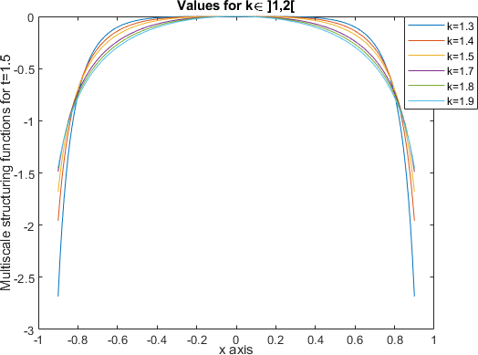
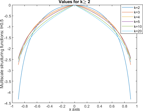
(a)	(b)

Figure 1: $b_{t}^{k}(x)$, $x\in]-1;~{}1[$: (a) for $t=1.5$ and $k\in]1;~{}2[$. (b) for $t=0.5$ and $k\geq 2$.

GM-GAN training procedure remains the same as traditional GANs. Specifically, the training procedure is carried out separately but simultaneously. The model takes as input some noise $z$ defined with a prior probability $p_{z}$, and then, attempts to learn the distribution of the generator $p_{g}$, by representing a function $G(z;\theta_{g})$ from $z$ to the data space. The discriminator network $D$ takes an input image $x$ and finds a function $D(x;\theta_{d})$ from $x$ to a single scalar, which is the probability that the image $x$ comes from $p_{data}$ which defines the origin of the sampled images. The output of the $D$ network returns a value close to $1$ if $x$ is a real image from $p_{data}$, and a value very close to $0$ if $x$ comes from $p_{g}$; otherwise. The main objective of network $D$ is to maximize $D(x)$ for an image coming from the true data distribution $p_{data}$, while minimizing $D(x)=D(G(z;\theta_{g}))$ for images generated from $p_{z}$ and not from $p_{data}$. The objective of the generator $G$ is to deceive the $D$ network, meaning to maximize $D(G(z;\theta_{g}))$. This is equivalent to minimize $1-D(G(z;\theta_{g}))$ as $D$ is a binary classifier. This conflict between these objectives is called the minimax game and formulated as follows:

$${\min\max E_{x\sim p_{data}(x)}[\log D(x)]+E_{z\sim p_{z}(z)}[\log(1-D(G(z;\theta_{g})))]}.$$

The case $p_{g}=p_{data}$ corresponds to the global optimum of the minimax game. Main contributions of the proposed GM-GAN rely on the equivariance property and non linearity characteristics brought out by group morphological convolutions and their ability to extract thin geometrical features, which lead to richer feature maps and a reduction of the amount training data.

For the GM-GAN generator, let $x$ be the input data into the morphological layer called Morphoblock. Then, $x$ goes first through a multiscale morphological erosion operation, followed by a multiscale morphological dilation. Afterwards, both erosion and dilation are followed by a linear convolution. The output of the PDE layer is obtained by a linear combination of the two outputs. The overall architecture of the GM-GAN generator is illustrated in Fig. 2.

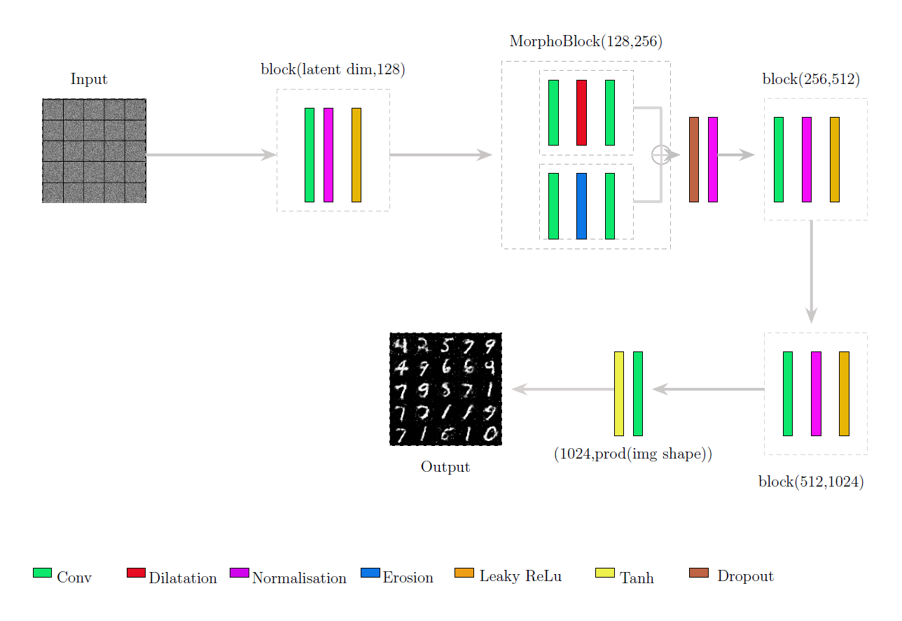
Figure 2: Architecture of GM-GAN generator.

6 Numerical experiments

GM-GAN and GAN are applied to MNIST dataset. MNIST database consists of $70,000$ black-and-white $28$x$28$ images that represent handwritten digits from $0$ to $9$. It is divided into a training set of $60,000$ images and a test set of $10,000$ images. Same training parameters are set for GM-GAN and GAN: number of epochs to $200$, the batch size to $64$, the latent space dimensionality to $100$, and the interval between image samples to $400$. Generated images with GM-GAN and GAN are displayed in Fig. 3.

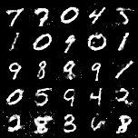
(a) GM-GAN: $70$

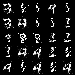
(b) GAN: $70$

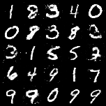
(c) GM-GAN: $90$

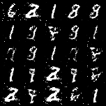
(d) GAN: $195$

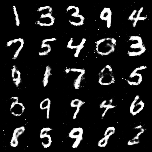
(e) GM-GAN: $71$

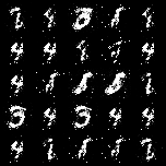
(f) GAN: $71$

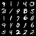
(g) GM-GAN: $91$

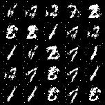
(h) GAN: $196$

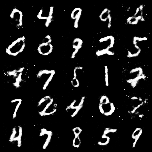
(i) GM-GAN: $72$

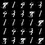
(j) GAN: $72$

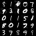
(k) GM-GAN: $92$

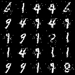
(l) GAN: $197$

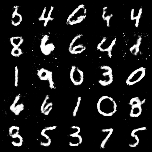
(m) GM-GAN:$73$

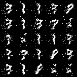
(n) GAN: $73$

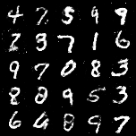
(o) GM-GAN: $93$

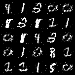
(p) GAN: $198$

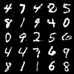
(q) GM-GAN: $74$

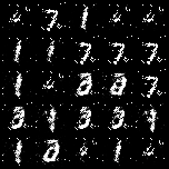
(r) GAN: $74$

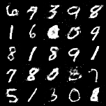
(s) GM-GAN: $94$

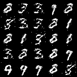
(t) GAN: $199$

Figure 3: Generated images from MNIST with GM-GAN and GAN on MNIST.

Clearly, we can say that generated images with GM-GAN are of higher quality than those produced by the traditional GAN. This can be seen by comparing images produced at epochs $70$ to $74$ with GM-GAN (Figs. 3(a), 3(e), 3(i), 3(m) and 3(q)) and ones generated at same epochs with GAN (Figs. 3(b), 3(f), 3(j), 3(n) and 3(r)). Indeed, some digits are clearly identifiable in the images generated by GM-GAN, whereas it is almost impossible to recognize the digits in those produced by GAN. Additionally, we also observe that the images generated with GM-GAN at epochs from $90$ to $94$ (Figs. 3(c), 3(g), 3(k), 3(o) and 3(s)) are also of better quality than those generated at the last five epochs with, that is at epochs from $195$ to $199$ (Figs. 3(d), 3(h), 3(l), 3(p) and 3(t)). To better display the quality of GM-GAN image generation, we zoom in on some areas in images generated at epochs $85$, $92$ and $96$ (Figs. 4-(a)-(b), (c)-(d) and (e)-(f); respectively) to demonstrate the realistic variations between the generated images of the same digit. This indicates that the GM-GAN model has a deep understanding of the sample characteristics and is capable of generalizing them beyond the specific examples it was trained on. This can be observed in Fig. 4-(b) with digits $3$ and $6$, Fig. 4-(d) with digits $2$ and $8$, and Fig. 4-(f) with digits $9$ and $7$.

 

(a)

 

(b)

 

(c)

 

(d)

 

(e)

 

(f)

Figure 4: Zoom in on images generated with GM-GAN at different epochs.

The complexity of GM-GAN is also reduced thanks to its equivariance property, thus eliminating the need to learn symmetries. This reduction is highlighted by halving the MNIST training dataset and comparing the generated images at epochs 36 and 42. The results of GM-GAN (Figs. 5(a), 5(e) respectively for epochs $36$ and $42$) once again demonstrate better image quality and greater variability in generated digits compared to GAN (Figs. 5(b), 5(f) respectively for epochs 36 and 42). These results underscore the importance of equivariance in morphological operators, thereby allowing for dataset reduction without significantly impacting generation results (see the images generated by GM-GAN at epochs $36$ and $42$ (Figs. 5(c), 5(g)) as well as those generated by GAN at these same epochs (Figs. 5(d), 5(h)) using the complete dataset).

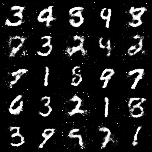
(a) GM-GAN(1/2)

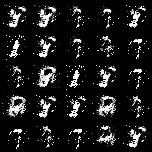
(b) GAN($1/2$)

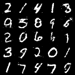
(c) GM-GAN

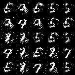
(d) GAN

(e) GM-GAN(1/2)

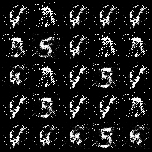
(f) GAN($1/2$)

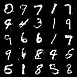
(g) GM-GAN

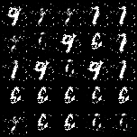
(h) GAN

Figure 5: Comparison between generated images at epoch $36$ (top line) and $42$ (bottom line) using $-$ Half MNIST dataset: (5(a),5(e)) MG-GAN, (5(b),5(f)) GAN. Whole MNIST dataset: (5(c),5(g)) MG-GAN, (5(d),5(h)) GAN.

Quantitative evaluations are also proposed using Frechet Inception Distance (FID) and Kullback-Leibler Divergence (KL). Low FID indicates high similarity between the generated and real data, which corresponds to good generation quality, and lower KL indicates better performance of the generative model, meaning that the distribution of generated data is closer to the distribution of real data. We report in Table 1 the quantitative results evaluated with KL and FID metrics for a sample of $10,432$ images generated with GM-GAN and GAN, which confirms the qualitative results discussed just above.

Models	Metrics
	KL divergence	FID metric
GM-GAN	$0.95$	$0.93$
GAN	$1.07$	$15.55$

Table 1: KL and FID metrics for GM-GAN an GAN.

As seen in Table 1, GM-GAN exhibits lower KL and much lower FID than GAN, suggesting that data generated with GM-GAN is closer, more realistic and trustworthy to the real data in terms of feature distribution.

7 Conclusion and perspectives

We have proposed here a geometric generative GM-GAN model based on PDE-G-CNNs and constructed from equivariant morphological operators and geometric image processing techniques. The proposed equivariant morphological PDE layers are composed of multiscale dilations and erosions without any need to approximate convolutions kernels, and meanwhile, group symmetries are defined on Lie groups allowing a geometrical interpretability of GM-GAN with left invariance properties. As shown by preliminary results on MNIST dataset, GM-GAN outperforms classical GAN. Indeed, thin image features are better extracted by accounting intrinsic geometric features at multiscale levels, and the network complexity is reduced. The proposed approach can be extended to more generative models. Ongoing works include applying GM-GAN on other datasets and designing fully equivariant generative models entirely based on PDE-G-CNNs.

References

- [1] Alvarez, L., Guichard, F., Lions, P.L., Morel, J.M.: Axioms and fundamental equations of image processing. Archive for rational mechanics and analysis 123, 199–257 (1993)
- [2] Angulo, J., Velasco-Forero., S.: Riemannian Mathematical Morphology. Pattern Recognition Letters 47, 93–101 (oct 2014)
- [3] Antoniou, A., Storkey, A., Edwards, H.: Data augmentation generative adversarial networks. arXiv preprint arXiv:1711.04340 (2017)
- [4] Arjovsky, M., Chintala, S., Bottou, L.: Wasserstein generative adversarial networks. In: International conference on machine learning. pp. 214–223. PMLR (2017)
- [5] Azagra, D., Ferrera, J.: Regularization by sup–inf convolutions on riemannian manifolds: An extension of lasry–lions theorem to manifolds of bounded curvature. Journal of Mathematical Analysis and Applications 423(2), 994–1024 (mar 2015)
- [6] Balan, V., Stojanov, J.: Finslerian-type GAF extensions of the riemannian framework in digital image processing. Filomat 29(3), 535–543 (2015). https://doi.org/10.2298/fil1503535b
- [7] Balogh, Z.M., Calogero, A., Pini, R.: The hopf–lax formula in carnot groups: a control theoretic approach. Calculus of Variations and Partial Differential Equations 49(3-4), 1379–1414 (may 2013)
- [8] Balogh, Z.M., Engulatov, A., Hunziker, L., Maasalo, O.E.: Functional inequalities and Hamilton–Jacobi equations in geodesic spaces. Potential analysis (2012)
- [9] Bardi, M., Evans, L.C.: On Hopf’s formulas for solutions of Hamilton-Jacobi equations. Nonlinear Analysis, Theory, Methods and Applications 8(11), 1373–1381 (jan 1984)
- [10] Barles, G.: Existence results for first order hamilton jacobi equations. Annales de l’Institut Henri Poincare (C) Non Linear Analysis 1(5), 325–340 (sep 1984). https://doi.org/10.1016/s0294-1449(16)30415-2
- [11] Bekkers, E.: B-Spline CNNs on Lie Groups. In: International Conference on Learning Representations (2019)
- [12] Bekkers, E.J., Lafarge, M.W., Veta, M., Eppenhof, K.A., Pluim, J.P., Duits, R.: Roto-translation covariant convolutional networks for medical image analysis. In: Medical Image Computing and Computer Assisted Intervention – MICCAI 2018: 21st International Conference, Proceedings, Part I. pp. 440–448. Granada, Spain (Sep 2018)
- [13] Bellaard, G., Bon, D.L., Pai, G., Smets, B.M., Duits, R.: Analysis of (sub-)Riemannian PDE-G-CNNs. Journal of Mathematical Imaging and Vision pp. 1–25 (2023)
- [14] Brockett, R.W., Maragos, P.: Evolution Equations for Continuous-Scale Morphological Filtering. IEEE Transactions on Signal Processing 42(12), 3377–386 (December 1994)
- [15] Burger, M., Sawatzky, A., Steidl, G.: First order algorithms in variational image processing. Springer (2016)
- [16] Camilli, F., Maio, R.D., Iacomini, E.: A hopf-lax formula for hamilton-jacobi equations with caputo time-fractional derivative. Journal of Mathematical Analysis and Applications 477(2), 1019–1032 (sep 2019). https://doi.org/10.1016/j.jmaa.2019.04.069
- [17] Chen, M., Denoyer, L.: Multi-view generative adversarial networks. In: Machine Learning and Knowledge Discovery in Databases: European Conference, ECML PKDD 2017, Skopje, Macedonia, September 18–22, 2017, Proceedings, Part II 10. pp. 175–188. Springer (2017)
- [18] Chen, X., Duan, Y., Houthooft, R., Schulman, J., Sutskever, I., Abbeel, P.: Infogan: Interpretable representation learning by information maximizing generative adversarial nets. Advances in neural information processing systems 29 (2016)
- [19] Citti, G., Franceschiello, B., Sanguinetti, G., Sarti, A.: Sub-riemannian mean curvature flow for image processing. SIAM Journal on Imaging Sciences 9(1), 212–237 (jan 2016). https://doi.org/10.1137/15m1013572
- [20] Citti, G., Sarti, A.: A cortical based model of perceptual completion in the roto-translation space. Journal of Mathematical Imaging and Vision 24, 307–326 (2006)
- [21] Cohen, T., Welling, M.: Group Equivariant Convolutional Networks. In: International conference on machine learning. pp. 2990–2999. PMLR (2016)
- [22] Cohen, T.S., Geiger, M., Köhler, J., Welling, M.: Spherical CNNs. In: International Conference on Learning Representations (2018)
- [23] Cohen, T.S., Geiger, M., Weiler, M.: A general theory of equivariant cnns on homogeneous spaces. Advances in neural information processing systems 32 (2019)
- [24] Crandall, M.G., Ishii, H., Lions, P.L.: User’s guide to viscosity solutions of second order partial differential equations. Bulletin of the American mathematical society 27(1), 1–67 (1992)
- [25] Crandall, M.G., Lions, P.L.: On existence and uniqueness of solutions of hamilton-jacobi equations. Nonlin. Anal.: Theo. Meth. & Appli. 10(4), 353–370 (1986). https://doi.org/10.1016/0362-546x(86)90133-1
- [26] Diop, E.H.S., Mbengue, A., Manga, B., Seck, D.: Extension of Mathematical Morphology in Riemannian Spaces. In: Lecture Notes in Computer Science, pp. 100–111. Springer International Publishing (2021)
- [27] Donahue, J., Krähenbühl, P., Darrell, T.: Adversarial feature learning. arXiv preprint arXiv:1605.09782 (2016)
- [28] Donato, D.D.: The intrinsic hopf-lax semigroup vs. the intrinsic slope. Journal of Mathematical Analysis and Applications 523(2), 127051 (jul 2023). https://doi.org/10.1016/j.jmaa.2023.127051
- [29] Dubrovina-Karni, A., Rosman, G., Kimmel, R.: Multi-region active contours with a single level set function. IEEE transactions on pattern analysis and machine intelligence 37(8), 1585–1601 (2014)
- [30] Duits, R., Bekkers, E.J., Mashtakov, A.: Fourier transform on the homogeneous space of 3D positions and orientations for exact solutions to linear PDEs. Entropy 21(1), 38 (2019)
- [31] Duits, R., Burgeth, B.: Scale spaces on Lie groups. In: International Conference on Scale Space and Variational Methods in Computer Vision. pp. 300–312 (2007)
- [32] Durugkar, I., Gemp, I., Mahadevan, S.: Generative multi-adversarial networks. arXiv preprint arXiv:1611.01673 (2016)
- [33] Evans, L.C., Souganidis, P.E.: Differential games and representation formulas for solutions of hamilton-jacobi-isaacs equations. Indiana University Mathematics Journal 33(5), 773–797 (mar 1984). https://doi.org/10.21236/ada127758
- [34] Fadili, J., Kutyniok, G., Peyré, G., Plonka-Hoch, G., Steidl, G.: Guest editorial: mathematics and image analysis. Journal of Mathematical Imaging and Vision 52, 315–316 (2015)
- [35] Fathi, A.: The Weak KAM Theorem in Lagrangian Dynamics. Cambridge University Press (2008)
- [36] Franceschiello, B., Mashtakov, A., Citti, G., Sarti, A.: Geometrical optical illusion via sub-Riemannian geodesics in the roto-translation group. Differential Geometry and its Applications 65, 55–77 (2019)
- [37] Gauthier, J.: Conditional generative adversarial nets for convolutional face generation. Class project for Stanford CS231N: convolutional neural networks for visual recognition, Winter semester 2014(5), 2 (2014)
- [38] Gerken, J.E., Aronsson, J., Carlsson, O., Linander, H., Ohlsson, F., Petersson, C., Persson, D.: Geometric deep learning and equivariant neural networks. Artificial Intelligence Review 56(12), 14605–14662 (Jun 2023). https://doi.org/10.1007/s10462-023-10502-7
- [39] Goodfellow, I.: Generative Adversarial Networks. In: NIPS. p. 57 (2017)
- [40] Goodfellow, I., Pouget-Abadie, J., Mirza, M., Xu, B., Warde-Farley, D., Ozair, S., Courville, A., Bengio, Y.: Generative adversarial nets. Advances in neural information processing systems 27 (2014)
- [41] Gu, J., Wang, Z., Kuen, J., Ma, L., Shahroudy, A., Shuai, B., TingLiu, Wang, X., Wang, L., Wang, G., Cai, J., Chen, T.: Recent Advances in Convolutional Neural Networks. Pattern recognition 77, 354–377 (2018)
- [42] Hausman, K., Chebotar, Y., Schaal, S., Sukhatme, G., Lim, J.J.: Multi-modal imitation learning from unstructured demonstrations using generative adversarial nets. Advances in neural information processing systems 30 (2017)
- [43] Iizuka, S., Simo-Serra, E., Ishikawa, H.: Globally and locally consistent image completion. ACM Transactions on Graphics (ToG) 36(4), 1–14 (2017)
- [44] Im, D.J., Kim, C.D., Jiang, H., Memisevic, R.: Generating images with recurrent adversarial networks. arXiv preprint arXiv:1602.05110 (2016)
- [45] Isola, P., Zhu, J.Y., Zhou, T., Efros, A.A.: Image-to-image translation with conditional adversarial networks. In: Proceedings of the IEEE conference on computer vision and pattern recognition. pp. 1125–1134 (2017)
- [46] Janssen, M.H., Janssen, A.J., Bekkers, E.J., Bescós, J.O., Duits, R.: Design and processing of invertible orientation scores of 3D images. Journal of mathematical imaging and vision 60, 1427–1458 (2018)
- [47] Kurtek, S., Jermyn, I.H., Xie, Q., Klassen, E., Laga, H.: Elastic shape analysis of surfaces and images. In: Riemannian Computing in Computer Vision, pp. 257–277. Springer International Publishing (2016)
- [48] Ledig, C., Theis, L., Huszár, F., Caballero, J., Cunningham, A., Acosta, A., Aitken, A., Tejani, A., Totz, J., Wang, Z., et al.: Photo-realistic single image super-resolution using a generative adversarial network. In: Proceedings of the IEEE conference on computer vision and pattern recognition. pp. 4681–4690 (2017)
- [49] Lions, P.L.: Generalized solutions of Hamilton-Jacobi equations. Pitman Advanced Publishing Program, London (1982)
- [50] Liu, M.Y., Breuel, T., Kautz, J.: Unsupervised image-to-image translation networks. Advances in neural information processing systems 30 (2017)
- [51] Manfredi, J.J., Stroffolini, B.: A version of the HOPF-LAX formula in the Heisenberg group. Com. in Partial Differential Equations 27(5-6), 1139–1159 (2002)
- [52] Pierson, E., Daoudi, M., Tumpach, A.B.: A Riemannian Framework for Analysis of Human Body Surface. In: IEEE/CVF Winter Conference on Applications of Computer Vision, WACV. pp. 2763–2772. Waikoloa, HI, USA (Jan 2022). https://doi.org/10.48550/ARXIV.2108.11449
- [53] Radford, A., Metz, L., Chintala, S.: Unsupervised representation learning with deep convolutional generative adversarial networks. arXiv preprint arXiv:1511.06434 (2015)
- [54] Reed, S., Akata, Z., Yan, X., Logeswaran, L., Schiele, B., Lee, H.: Generative adversarial text to image synthesis. In: International conference on machine learning. pp. 1060–1069. PMLR (2016)
- [55] Ren, H., Chen, D., Wang, Y.: RAN4IQA: Restorative adversarial nets for no-reference image quality assessment. In: Proceedings of the AAAI conference on artificial intelligence (2018)
- [56] Romero, D., Bekkers, E., Tomczak, J., Hoogendoorn, M.: Attentive Group Equivariant Convolutional Networks. In: Proceedings of Machine Learning Research. pp. 8188–8199 (2020)
- [57] Sajjadi, M.S., Scholkopf, B., Hirsch, M.: Enhancenet: Single image super-resolution through automated texture synthesis. In: Proceedings of the IEEE international conference on computer vision. pp. 4491–4500 (2017)
- [58] Sapiro, G., Kimmel, R., Shaked, D., Kimia, B.B., Bruckstein, A.M.: Implementing continuous-scale morphology via curve evolution. Pattern Recognition 26(9), 1363–1372 (1993)
- [59] Shih, F.: Image processing and mathematical morphology : fundamentals and applications. CRC Press, Boca Raton (2009)
- [60] Smets, B.M.N., Portegies, J., Bekkers, E.J., Duits, R.: PDE-Based Group Equivariant Convolutional Neural Networks. Journal of Mathematical Imaging and Vision 65(1), 209–239 (2022)
- [61] Su, J., Kurtek, S., Klassen, E., Srivastava, A.: Statistical analysis of trajectories on Riemannian manifolds: Bird migration, hurricane tracking and video surveillance. The Annals of Applied Statistics 8(1) (Mar 2014). https://doi.org/10.1214/13-aoas701
- [62] Tian, C., Zhang, Y., Zuo, W., Lin, C.W., Zhang, D., Yuan, Y.: A Heterogeneous Group CNN for Image Super-Resolution. IEEE Transactions on Neural Networks and Learning Systems pp. 1–13 (2024)
- [63] Vukotić, V., Raymond, C., Gravier, G.: Generative adversarial networks for multimodal representation learning in video hyperlinking. In: Proceedings of the 2017 ACM on International Conference on Multimedia Retrieval. pp. 416–419 (2017)
- [64] Welk, M., Weickert, J.: Pde evolutions for m-smoothers: from common myths to robust numerics. In: International Conference on Scale Space and Variational Methods in Computer Vision. pp. 236–248. Springer (2019)
- [65] Winkels, M., Cohen, T.S.: 3d G-CNNs for pulmonary nodule detection. In: Medical Imaging with Deep Learning (2018)
- [66] Xu, Q., Qin, Z., Wan, T.: Generative cooperative net for image generation and data augmentation. In: Integrated Uncertainty in Knowledge Modelling and Decision Making: 7th International Symposium, IUKM 2019, Nara, Japan, March 27–29, 2019, Proceedings 7. pp. 284–294. Springer (2019)
- [67] Xu, X., Sun, D., Pan, J., Zhang, Y., Pfister, H., Yang, M.H.: Learning to super-resolve blurry face and text images. In: Proceedings of the IEEE international conference on computer vision. pp. 251–260 (2017)
- [68] Yeh, R.A., Chen, C., Yian Lim, T., Schwing, A.G., Hasegawa-Johnson, M., Do, M.N.: Semantic image inpainting with deep generative models. In: Proceedings of the IEEE conference on computer vision and pattern recognition (2017)
- [69] Younes, L.: Shapes and Diffeomorphisms. Springer Berlin Heidelberg (May 2019)
- [70] Yu, J., Lin, Z., Yang, J., Shen, X., Lu, X., Huang, T.S.: Generative image inpainting with contextual attention. In: Proceedings of the IEEE conference on computer vision and pattern recognition. pp. 5505–5514 (2018)
- [71] Zhang, H., Xu, T., Li, H., Zhang, S., Wang, X., Huang, X., Metaxas, D.N.: Stackgan: Text to photo-realistic image synthesis with stacked generative adversarial networks. In: Proceedings of the IEEE international conference on computer vision. pp. 5907–5915 (2017)
- [72] Zhu, J.Y., Zhang, R., Pathak, D., Darrell, T., Efros, A.A., Wang, O., Shechtman, E.: Toward multimodal image-to-image translation. Advances in neural information processing systems 30 (2017)