Establishing a leader in a pairwise comparisons method

Abstract

Like electoral systems, decision-making methods are also vulnerable to manipulation by decision-makers. The ability to effectively defend against such threats can only come from thoroughly understanding the manipulation mechanisms. In the presented article, we show two algorithms that can be used to launch a manipulation attack. They allow for equating the weights of two selected alternatives in the pairwise comparison method and, consequently, choosing a leader. The theoretical considerations are accompanied by a Monte Carlo simulation showing the relationship between the size of the PC matrix, the degree of inconsistency, and the ease of manipulation. This work is a continuation of our previous research published in the paper [30].

1 Introduction

The pairwise comparisons method (PC) constitutes a convenient and broadly applied tool for a complexity reduction in the multiple criteria decision-making (MCDM) frameworks such as the Analytic Hierarchy Process (AHP) [27], Best-Worst Method (BWM) [26], MACBETH [1], or PROMETHEE [6].

In recent decades, many researchers studied PC methods intensively concerning its consistency, optimal derivation of a priority vector, priority vector’s desirable properties, and other aspects, see e.g. [10, 19, 20, 25]. Since the objective of a PC method is to rank compared objects (usually alternatives or criteria) from the best to the worst, it may happen that an expert deliberately distorts one or more pairwise comparisons to promote a selected object, see e.g. [21, 32, 33]. In particular, the problem of preference manipulation has gained attention in the context of group decision-making (see, e.g. [11, 12, 23, 24, 28]), or electoral systems analysis ([5, 13, 15]). The studies above focused on manipulation detection, various anti-manipulation strategies (mainly through some penalization brought upon a manipulator), or an estimation of manipulation robustness. Prevention of manipulation was discussed, e.g., in [21, 29, 31].

In particular, a recent study by Kułakowski et al. [21] introduced two heuristics enabling the detection of manipulators and minimizing their effect on the group consensus by diminishing their weights. The first heuristic is based on the assumption that manipulators will provide judgments that can be considered outliers concerning those of the other experts in the group. The second heuristic assumes dishonest judgments are less consistent than the average consistency of the group.

The presented study is a follow-up of the work by Szybowski et al. [30], where an algorithm balancing the weights of two given alternatives of a pairwise comparisons matrix (EQ algorithm) has been introduced. This study aims to introduce a modification of the EQ algorithm that is more efficient in the case of its multiple uses and to propose two other algorithms based on the EQ algorithm (greedy and bubble sort) capable of altering the best alternative by a minimal change in elements of an original additive PC matrix. Further, we define the so-called Average Ranking Stability Index (ARSI) as a measurement of ranking manipulation’s difficulty. Last but not least, we perform Monte Carlo simulations to analyze relationships between the size of a PC matrix, its inconsistency, and the degree of manipulation difficulty given by the ARSI. In the proposed method, we use PC matrix orthogonalization. We can also use this technique in procedures to increase the consistency of PC matrices [4, 17].

The paper is organized as follows: Section 2 provides preliminaries, Section 3 presents new algorithms, and Section 4 includes numerical (Monte Carlo) simulations. Conclusions close the article.

2 Preliminaries

2.1 Multiplicative and additive pairwise comparisons systems

Let $E=\{e_{1},\ldots,e_{n}\}$ be a finite set of alternatives, $n\geq 2$, and the goal is to rank all alternatives from the best to the worst by pairwise comparisons.

• In the multiplicative pairwise comparisons (MPCs) framework, an expert expresses his/her judgment of a relative preference (importance) of $e_{i}$ and $e_{j}$ by the value $m_{ij}\in\mathbb{R^{+}}$, where $m_{ij}>1$ means $e_{i}$ is preferred over $e_{j}$, and $m_{ij}=1$ denotes equal preference of both alternatives.

  
  

  MPCs are reciprocal, if:

  $m_{ij}=1/m_{ji};\forall i,j\in\{1,...,n\}$.

  MPCs are consistent, if:

  $m_{ij}\cdot m_{jk}=m_{ik};\forall i,j\in\{1,...,n\}$.

  All MPCs are conveniently arranged into an $n\times n$ multiplicative pairwise comparisons matrix $M=[m_{ij}]$, and a priority vector (vector of alternatives’ weights) is then calculated by the eigenvector [27] or the (row) geometric mean method [9].

  Inconsistency of an MPC matrix $M$ can be estimated by the consistency index ($CI$) [27]:

  $CI(M)=\dfrac{\lambda_{max}-n}{n-1}$, where $\lambda_{max}$ denotes the maximal eigenvalue of $M$. Of course, there are a number of other methods for determining the degree of inconsistency of a PC matrix such as the Koczkodaj’s index [18], Kazibudzki’s Square Logarithm Deviations index [16] or Barzilai’s error [2]. A comprehensive review of methods for measuring inconsistency in PC matrices can be found in [7]. In addition to the inconsistency of the PC matrix, the incompleteness index can also be determined [22].

  
  

• In the additive pairwise comparisons (APCs) framework, an expert expresses his/her judgment of a relative preference (importance) of $e_{i}$ and $e_{j}$ by the value $a_{ij}\in\mathbb{R}$, where $a_{ij}>0$ means $e_{i}$ is preferred over $e_{j}$, and $a_{ij}=0$ denotes equal preference of both alternatives.

  
  

  APCs are reciprocal, if:

  $a_{ij}=-a_{ji};\forall i,j\in\{1,...,n\}$.

  APCs are consistent, if:

  $a_{ij}+a_{jk}=a_{ik};\forall i,j\in\{1,...,n\}$.

  All APCs are conveniently arranged into an $n\times n$ additive pairwise comparisons matrix $A=[a_{ij}]$, and a priority vector (vector of alternatives’ weights) is then calculated by the row arithmetic mean method [3].

Multiplicative and additive pairwise comparisons share the same group structure (are isomorphic) [8] and can be easily converted into each other by exponential and logarithmic transformations respectively:

$a_{ij}=log(m_{ij}),m_{ij}=exp(a_{ij})$

Both MPC and APC systems have they advantages. While the MPCs are based on ratios, which are natural to human thinking, APCs enable to use rich mathematical apparatus of linear algebra, which is especially convenient for theoretical considerations [14].

The space

$$\mathcal{A}:=\{[a_{ij}]:\ \forall i,j\in\{1,\ldots,n\}\ a_{ij}\in\mathbb{R}\textnormal{ and }a_{ij}+a_{ji}=0\},$$

is a linear space of additive pairwise comparisons matrices (PCMs). Recall that any linear space is endowed with a (orthogonal) basis and that for two given $n\times n$ matrices $A$ and $B$ their standard Frobenius product is defined as follows:

$$\langle A,B\rangle=\sum_{k=1}^{n}\sum_{l=1}^{n}a_{kl}b_{kl},$$

which induces the Frobenius norm

$$||A||=\sqrt{\langle A,A\rangle}$$

and the Frobenius distance

$$d(A,B)=||A-B||.$$

2.2 Ranking stability index

In the additive pairwise comparisons method it is usually assumed that the elements of a PCM fall within a certain range $[-M,M]$, for a fixed $M>0$. In this case, according to [30] the Ranking Stability Index of alternatives $e_{i}$ and $e_{j}$ has been defined as

$$RSI_{ij}^{M}=\frac{|\sum_{k=1}^{n}(a_{ik}-a_{jk})|}{2M}.$$

This index expresses a rescaled distance of the weights of the $i$-th and $j$-th alternatives.

The Ranking Stability Index for a PCM $A$ is given by the formula

$$RSI^{M}(A)=\min_{1\leq i\leq j\leq n}RSI_{ij}^{M},$$

and it measures the ease of the easiest manipulation.

However, sometimes the decision process is more complicated and some attempts of manipulations may not be that obvious. Therefore, it could be useful to define the Average Ranking Stability Index for $A$ as follows:

$$ARSI^{M}(A)=\frac{2}{n(n-1)^{2}}\sum_{1\leq i\leq j\leq n}RSI_{ij}^{M}.$$

Since for all $i,j$

$$0\leq RSI_{ij}^{M}\leq n-1,$$

we immediately get

$$0\leq ARSI^{M}\leq 1.$$

3 Establishing a leading alternative

3.1 Equating two alternatives

Let us recall the algorithm of finding the best approximation of a given PCM $A$, which equates the weights of two given alternatives $e_{i}$ and $e_{j}$ (for $i<j$). This algorithm has been introduced in [30] and we will denote it by EQ($A,i,j$).

In the beginning, we consider the case $i=1$ and $j=2$.

For this purpose we define:

• the tie space ${\cal A}_{12}$, i.e. the $\frac{n^{2}-n-2}{2}$-dimensional subspace of all additive PCMs which induce the ranking such that alternatives $1$ and $2$ are equal:

  $${\cal A}_{12}=\left\{A\in{\cal A}:\sum_{k=1}^{n}a_{1k}=\sum_{k=1}^{n}a_{2k}\right\},$$

• the set

  $$Z_{12}:=\{(q,r):\ 3\leq q<r\leq n\}.$$

We define a basis for the tie space ${\cal A}_{12}$ which consists of additive PCMs $C^{qr}$ ($(q,r)\in Z_{12}$), $E^{1}$, $F^{p}$ ($p\in\{3,\ldots,n\}$) and $G^{p}$ ($p\in\{3,\ldots,n-1\}$), whose elements are given by

$$c_{kl}^{qr}=\left\{\begin{array}[]{rl}1,&k=q,\ l=r\\ -1,&k=r,\ l=q\\ 0,&\textnormal{otherwise}\end{array}\right..$$

$$e_{kl}^{1}=\left\{\begin{array}[]{rl}1,&(k=1,\ l=2)\\ -1,&(k=2,\ l=1)\\ 2,&k=2,\ l=n\\ -2,&k=n,\ l=2\\ 0,&\textnormal{otherwise}\end{array}\right.,$$

$$f_{kl}^{p}=\left\{\begin{array}[]{rl}1,&(k=1,\ l=p)\textnormal{ or }(k=2,\ l=n)\\ -1,&(k=p,\ l=1)\textnormal{ or }(k=n,\ l=2)\\ 0,&\textnormal{otherwise}\end{array}\right.,$$

and

$$g_{kl}^{p}=\left\{\begin{array}[]{rl}1,&(k=2,\ l=p)\textnormal{ or }(k=n,\ l=2)\\ -1,&(k=p,\ l=2)\textnormal{ or }(k=2,\ l=n)\\ 0,&\textnormal{otherwise}\end{array}\right..$$

Theorem 1 (Theorem 5,[30]).

A family of matrices

$${\cal B}=\{B^{p}\}_{p=1}^{\frac{n^{2}-n}{2}-1}:=\{C^{qr}\}_{(q,r)\in Z_{12}}\cup\{E^{1}\}\cup\{F^{p}\}_{p=3}^{n}\cup\{G^{p}\}_{p=3}^{n-1}$$ (1)

is a basis of ${\cal A}_{12}$.

Next, we apply a standard Gram-Schmidt process to the basis

$$B^{1},\ldots,B^{\frac{n^{2}-n}{2}-1}$$

of the vector space ${\cal A}_{12}$ equipped with a standard Frobenius inner product $\langle\cdot,\cdot\rangle$ and we obtain a pairwise orthogonal basis

$$H^{1},\ldots,H^{\frac{n^{2}-n}{2}-1}$$ (2)

as follows:

$$H^{1} = B^{1},$$

$$H^{2} = B^{2}-\frac{\langle H^{1},B^{2}\rangle}{\langle H^{1},H^{1}\rangle}H^{1},$$

$$H^{3} = B^{3}-\frac{\langle H^{1},B^{3}\rangle}{\langle H^{1},H^{1}\rangle}H^{1}-\frac{\langle H^{2},B^{3}\rangle}{\langle H^{2},H^{2}\rangle}H^{2},$$

$$\cdots = \cdots$$

$$H^{\frac{n^{2}-n}{2}-1} = B^{\frac{n^{2}-n}{2}-1}-\sum_{p=1}^{\frac{n^{2}-n}{2}-2}\frac{\langle H^{p},B^{\frac{n^{2}-n}{2}-1}\rangle}{\langle H^{p},H^{p}\rangle}H^{p}.$$

Example 2.

Consider $n=4$. Then the dimension of ${\cal A}_{12}$ is $\frac{n^{2}-n-2}{2}=5$.

Since $Z_{12}=\{(3,4)\}$, we get the following basis of ${\cal A}_{12}$:

$B^{1}=C^{34}=\left(\begin{array}[]{cccc}0&0&0&0\\ 0&0&0&0\\ 0&0&0&1\\ 0&0&-1&0\end{array}\right),$ $B^{2}=E^{1}=\left(\begin{array}[]{cccc}0&1&0&0\\ -1&0&0&2\\ 0&0&0&0\\ 0&-2&0&0\end{array}\right),$

$B^{3}=F^{3}=\left(\begin{array}[]{cccc}0&0&1&0\\ 0&0&0&1\\ -1&0&0&0\\ 0&-1&0&0\end{array}\right),$ $B^{4}=F^{4}=\left(\begin{array}[]{cccc}0&0&0&1\\ 0&0&0&1\\ 0&0&0&0\\ -1&-1&0&0\end{array}\right),$

$B^{5}=G^{3}=\left(\begin{array}[]{cccc}0&0&0&0\\ 0&0&1&-1\\ 0&-1&0&0\\ 0&1&0&0\end{array}\right).$

Application of the Gram-Schmidt process to this basis results in an orthogonal basis

$$H^{1}=B^{1} = \left(\begin{array}[]{cccc}0&0&0&0\\ 0&0&0&0\\ 0&0&0&1\\ 0&0&-1&0\end{array}\right),$$

$$\langle H^{1},B^{2}\rangle=0\Rightarrow H^{2}=B^{2} = \left(\begin{array}[]{cccc}0&1&0&0\\ -1&0&0&2\\ 0&0&0&0\\ 0&-2&0&0\end{array}\right),$$

$$\langle H^{1},B^{3}\rangle=0,\ \langle H^{2},B^{3}\rangle=4,\ \langle H^{2},H^{2}\rangle=10 \Rightarrow$$

$$\Rightarrow H^{3} = \left(\begin{array}[]{cccc}0&-\frac{2}{5}&1&0\\ \frac{2}{5}&0&0&\frac{1}{5}\\ -1&0&0&0\\ 0&-\frac{1}{5}&0&0\end{array}\right),$$

$$\langle H^{1},B^{4}\rangle=0,\ \langle H^{2},B^{4}\rangle=4,\ \langle H^{3},B^{4}\rangle=\frac{2}{5},\ \langle H^{3},H^{3}\rangle=\frac{12}{5} \Rightarrow$$

$$\Rightarrow H^{4} = \left(\begin{array}[]{cccc}0&-\frac{1}{3}&-\frac{1}{6}&1\\ \frac{1}{3}&0&0&\frac{1}{6}\\ \frac{1}{6}&0&0&0\\ -1&-\frac{1}{6}&0&0\end{array}\right),$$

$$\langle H^{1},B^{5}\rangle=0,\ \langle H^{2},B^{5}\rangle=-4,\ \langle H^{3},B^{5}\rangle=-\frac{2}{5}\ \langle H^{4},B^{5}\rangle=-\frac{1}{3},\$$

$$\langle H^{4},H^{4}\rangle=\frac{7}{3}\Rightarrow H^{5} = \left(\begin{array}[]{cccc}0&\frac{2}{7}&\frac{1}{7}&\frac{1}{7}\\ -\frac{2}{7}&0&1&-\frac{1}{7}\\ -\frac{1}{7}&-1&0&0\\ -\frac{1}{7}&\frac{1}{7}&0&0\end{array}\right).$$

Now, for an additive PCM $A$ we find its projection $A^{\prime}$ onto the subspace ${\cal A}_{12}$ as a linear combination of the orthogonal basis vectors

$$H^{1},\ldots,H^{\frac{n^{2}-n}{2}-1}:$$

i.e.

$$A^{\prime}=\varepsilon_{1}H^{1}+\ldots\varepsilon_{\frac{n^{2}-n}{2}-1}H^{\frac{n^{2}-n}{2}-1},$$

where the factors

$$\varepsilon_{1},\ldots,\varepsilon_{\frac{n^{2}-n}{2}-1}$$

are expressed by formulas:

$$\varepsilon_{k}=\frac{\langle A,H^{k}\rangle}{\langle H^{k},H^{k}\rangle},\ k=1,\ldots,\frac{n^{2}-n}{2}-1.$$

Thus, the algorithm EQ($A,1,2$) can be written in a very simple way:

1. ${\displaystyle A^{\prime}:=\sum_{k=1}^{\frac{n^{2}-n}{2}-1}\frac{\langle A,H^{k}\rangle}{\langle H^{k},H^{k}\rangle}H^{k};}$

2. Return($A^{\prime}$);

Now, let us consider the general case, i.e. $1\leq i<j\leq n$.

Remark 3.

If $P$ is a matrix of permutation of the $p$-th and $q$-th coordinates, then

$$||PA-PB||=||A-B||,$$

and

$$||AP-BP||=||A-B||,$$

for each PCMs $A$ and $B$.

Proof.

The thesis follows from the fact that we get $P(A-B)$ (and $(A-B)P$) from $A-B$ by the permutation of the $p$-th and the $q$-th rows (columns). ∎

Thus, in order to find the closest matrix to $A$ equating the $i$-th and $j$-th alternatives, we first permute alternatives $\{i,j\}$ with $\{1,2\}$, then perform EQ($A,1,2$), and finally permute $\{1,2\}$ with $\{i,j\}$.

Let us define the permutation matrix $P_{ij}=[p_{kl}]_{k,l=1}^{n}$.

If $i=1$ and $j\neq 2$, then we put:

$$p_{kl}=\left\{\begin{array}[]{cl}1,&(k,l)\in\{(2,j),(j,2)\}\textnormal{ or }k=l\not\in\{2,j\}\\ 0,&\textnormal{otherwise,}\end{array}\right.$$

If $i\neq 1$ and $j=2$, then we put:

$$p_{kl}=\left\{\begin{array}[]{cl}1,&(k,l)\in\{(1,i),(i,1)\}\textnormal{ or }k=l\not\in\{1,i\}\\ 0,&\textnormal{otherwise,}\end{array}\right.$$

If $i\neq 1$ and $j\neq 2$, then we put:

$$p_{kl}=\left\{\begin{array}[]{cl}1,&(k,l)\in\{(1,i),(i,1),(2,j),(j,2)\}\textnormal{ or }k=l\not\in\{1,2,i,j\}\\ 0,&\textnormal{otherwise.}\end{array}\right.$$

SInce for each $(i,j)\neq(1,2)$ the matrix $P_{ij}$ is orthogonal we have

Remark 4.

$P_{ij}^{-1}=P_{ij}^{T}=P_{ij}$.

We are ready to introduce the general algorithm EQ($A,i,j$):

1. If $(i,j)\neq(1,2)$, then $A:=P_{ij}AP_{ij}$;

2. $A$:=EQ($A,1,2$);

3. If $(i,j)\neq(1,2)$, then $A:=P_{ij}AP_{ij}$;

4. Return($A$).

Notice that the above procedure improves the algorithm introduced in Szybowski2023aomo [30], because:
1. we allow $j=n$,
2. we always use the same orthogonal base $H^{1},\ldots,H^{\frac{n^{2}-n}{2}-1}$ (which is important if we have to run EQ($i,j$) several times for different $i$ and $j$).

Theorem 5 (Theorem 9, [30]).

Let $A=[a_{kl}]\in{\cal{A}}$, $i,j\in\{1,\ldots,n\}$, and $A^{\prime}=[a^{\prime}_{kl}]$ be the orthogonal projection of $A$ onto ${\cal A}_{ij}$. Then
(1) For each $k\not\in\{i,j\}$

$$\sum_{l=1}^{n}a^{\prime}_{kl}=\sum_{l=1}^{n}a_{kl},$$ (8)

(2)

$$\sum_{l=1}^{n}a^{\prime}_{il}=\sum_{l=1}^{n}a^{\prime}_{jl}=\frac{\sum_{l=1}^{n}a_{il}+\sum_{l=1}^{n}a_{jl}}{2}.$$ (9)

3.2 The algorithm for establishing a leading alternative in a PC method

Let us present the main algorithm of the paper.

Suppose we have a PCM $A$ and we want to promote the $p$-th alternative for the first place in the ranking.

3.2.1 The greedy algorithm

INPUT: $A,\ p$.

1. $q:=$ the number of the best alternative

2. If $p=q$ then return($A$);

3. Construct the basis (1);

4. Apply the Gram-Schmidt process to obtain the basis (2);

5. repeat
   

   • $A:=$EQ($A,p,q$);

   • $q:=$ the number of the best alternative;

   until ranking($p$) $=$ ranking($q$);
   

6. return($A$);

Example 6.

Let us consider a $4\times 4$ ($n=4$) PCM

$$A=\left(\begin{array}[]{cccc}0&1&2&9\\ -1&0&1&8\\ -2&-1&0&7\\ -9&-8&-7&0\end{array}\right).$$

The weights in a ranking vector obtained as the arithmetic means of elements of rows of $A$ are

$$w=(3,2,1,-6)^{T},$$

so the initial value of $q$ is 1.

Our goal is to promote the fourth alternative ($p=4$) to the first position in a ranking.

In the example the alternative number 4 is definitely the worst one, so the algorithm EQ must run $n-1=3$ times, which is the maximal possible number of iterations.

We construct the basis $B^{1},\ldots,B^{5}$. Next, we apply the Gram-Shmidt procedure to obtain basis $H^{1},\ldots,H^{5}$. Both bases are described in Ex. 2.

THE 1ST ITERATION OF THE LOOP:

We run EQ($A,1,4$), i.e. we calculate:

$$P_{14}=\left(\begin{array}[]{cccc}1&0&0&0\\ 0&0&0&1\\ 0&0&1&0\\ 0&1&0&0\end{array}\right).$$

$$A^{(2)}=P_{14}AP_{14}=\left(\begin{array}[]{cccc}0&9&2&1\\ -9&0&-7&-8\\ -2&7&0&-1\\ -1&8&1&0\end{array}\right).$$

$$A^{(3)}=\textnormal{EQ}(A^{(2)},1,2)=\left(\begin{array}[]{cccc}0&0&-2.5&-3.5\\ 0&0&-2.5&-3.5\\ 2.5&2.5&0&-1\\ 3.5&3.5&1&0\end{array}\right).$$

$$A^{(4)}=P_{14}A^{(3)}P_{14}=\left(\begin{array}[]{cccc}0&-3.5&-2.5&0\\ 3.5&0&1&3.5\\ 2.5&-1&0&2.5\\ 0&-3.5&-2.5&0\end{array}\right).$$

The ranking vector for $A^{(4)}$ is

$$w=(-1.5,2,1,-1.5)^{T},$$

so the next value of $q$ is 2.

THE 2ND ITERATION OF THE LOOP:

We run EQ($A^{(4)},2,4$), i.e. we calculate:

$$P_{24}=\left(\begin{array}[]{cccc}0&0&0&1\\ 0&1&0&0\\ 0&0&1&0\\ 1&0&0&0\end{array}\right).$$

$$A^{(5)}=P_{24}A^{(4)}P_{24}=\left(\begin{array}[]{cccc}0&-3.5&-2.5&0\\ 3.5&0&1&3.5\\ 2.5&-1&0&2.5\\ 0&-3.5&-2.5&0\end{array}\right).$$

$$A^{(6)}=\textnormal{EQ}(A^{(5)},1,2)=\left(\begin{array}[]{cccc}0&0&-0.75&1.75\\ 0&0&-0.75&1.75\\ 0.75&0.75&0&2.5\\ -1.75&-1.75&-2.5&0\end{array}\right).$$

$$A^{(7)}=P_{24}A^{(6)}P_{24}=\left(\begin{array}[]{cccc}0&-1.75&-2.5&-1.75\\ 1.75&0&-0.75&0\\ 2.5&0.75&0&0.75\\ 1.75&0&-0.75&0\end{array}\right).$$

The ranking vector for $A^{(7)}$ is

$$w=(-1.5,0.25,1,0.25)^{T},$$

so the next value of $q$ is 3.

THE 3RD ITERATION OF THE LOOP:

We run EQ($A^{(7)},3,4$), i.e. we calculate:

$$P_{34}=\left(\begin{array}[]{cccc}0&0&1&0\\ 0&0&0&1\\ 1&0&0&0\\ 0&1&0&0\end{array}\right).$$

$$A^{(8)}=P_{34}A^{(7)}P_{34}=\left(\begin{array}[]{cccc}0&0.75&2.5&0.75\\ -0.75&0&1.75&0\\ -2.5&-1.75&0&-1.75\\ -0.75&0&1.75&0\end{array}\right).$$

$$A^{(9)}=\textnormal{EQ}(A^{(8)},1,2)=\left(\begin{array}[]{cccc}0&0&2.125&0.375\\ 0&0&2.125&0.375\\ -2.125&-2.125&0&-1.75\\ -0.375&-0.375&1.75&0\end{array}\right).$$

$$A^{(10)}=P_{34}A^{(9)}P_{34}=\left(\begin{array}[]{cccc}0&-1.75&-2.125&-2.125\\ 1.75&0&-0.375&-0.375\\ 2.125&0.375&0&0\\ 2.125&0.375&0&0\end{array}\right).$$

The ranking vector for $A^{(10)}$ is

$$w=(-1.5,0.25,0.625,0.625)^{T},$$

so the final value of $q$ is 3. The weights of alternatives $p$ and $q$ are now equal and the highest, so the algorithm breaks. The output matrix is $A^{10)}$.

Notice that the chosen alternative is not a sole leader in the ranking. However, even the slightest correction of the element $a_{pq}$ in favor of the alternative $p$ may change that. For example, if we put $a_{34}=-0.1$ (and, respectively $a_{43}=0.1$), then we get "the winning ranking":

$$w=(-1.5,0.25,0.6,0.65)^{T}.$$

3.2.2 The bubble algorithm

As Example 6 shows, the greedy algorithm has some disadvantages. It is fast on average, however, if the preferred alternative is on the bottom of the ranking we may need to run a loop $n-1$ times. Secondly, the whole procedure may competely reverse the ranking, which is undesirable.

Therefore, we suggest an alternative algorithm, which promotes a chosen alternative stepwise.

INPUT: $A,\ p$.

1. $q:=$ the number of the best alternative

2. If $p=q$ then return($A$);

3. Construct the basis (1);

4. Apply the Gram-Shmidt process to obtain the basis (2);

5. repeat
   

   • $A:=$EQ($A,p,q$);

   • $q:=$ the number of the alternative directly ahead of the alternative $p$ in the ranking;

   until ranking($p$) $=$ ranking($q$);
   

6. return($A$);

Example 7.

Consider once more the matrix $A$ from the example 6. The output matrix after running the bubble algorithm is of the form:

$$A^{(10)}=\left(\begin{array}[]{cccc}0&1.625&3.875&0\\ -1.625&0&2.25&-1.625\\ -3.875&-2.25&0&-3.875\\ 0&1.625&3.875&0\end{array}\right),$$

and the final ranking vector is

$$w=(1.375,-0.25,-2.5,1.375)^{T},$$

so the fourth alternative moved up to the first position (ex aequo with the first one), but the relative positions of the other alternatives did not change.

4 Monte Carlo Simulation

For Monte Carlo testing, we generated $2500$ preference profiles within which the relative priority of a pair of alternatives ranges from $[1/9,9]$. The number of alternatives ranges from $5$ to $9$, i.e. for five alternatives we generate $500$ random profiles, for 6 alternatives - $500$ profiles were prepared, etc.

Based on the drawn preference profiles, we created random pairwise comparison matrices (PCM) in such a way that for a preference profile

$$w=\left(w(a_{1}),\ldots,w(a_{n})\right)^{T}$$

a $C_{\alpha}$ is a $n\times n$ PCM in the form

$$C_{\alpha}=\left(\begin{array}[]{ccccc}1&c_{1,2}r_{1,2}&c_{1,3}r_{1,3}&\cdots&c_{1,n}r_{1,n}\\ c_{2,1}r_{2,1}&1&c_{2,3}r_{2,3}&\cdots&c_{2,n}r_{2,n}\\ \vdots&\cdots&\ddots&\cdots&\vdots\\ \vdots&\cdots&\cdots&\ddots&\vdots\\ c_{n,1}r_{n,1}&c_{n,2}r_{n,2}&\cdots&c_{n,n-1}r_{n,n-1}&1\end{array}\right),$$

where

$$c_{ij}=\frac{w(a_{i})}{w(a_{j})},$$

and $r_{ij}$ is a real number randomly selected from $[1/\alpha,\alpha]$ for $i,j=1,\ldots,n$. Thus, by increasing the value of $\alpha$, we effectively increase the inconsistency of $C_{\alpha}$. We created matrices in the form of $C_{\alpha}$ for all $2,500$ random preference profiles and for all $\alpha$ values from the set $\{1,1.1,1.2,\ldots,4.9,5\}$. In the end, we generated $102,500=2,500\times 41$ random PCM matrices with varying degrees of inconsistency and dimensions ranging from $5\times 5$ to $9\times 9$. All generated matrices were used as input to both greedy (Sec. 3.2.1) and bubble algorithms (Sec. 3.2.2).

(a) Greedy algorithm, LBN strategy

(b) Greedy algorithm, LBR strategy

(c) Bubble algorithm, LBN strategy

(d) Bubble algorithm, LBR strategy

Figure 1: Number of iterations vs. number of alternatives

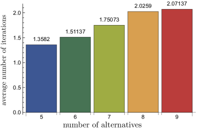
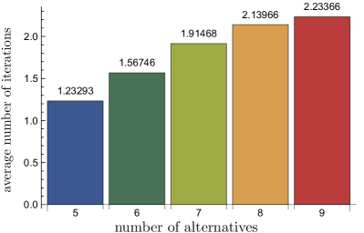
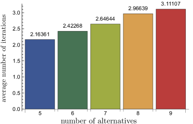
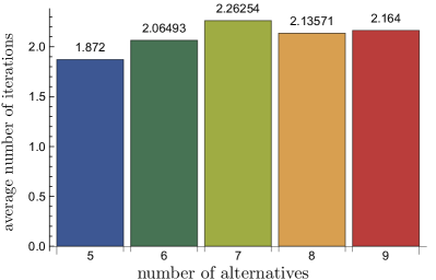
For both algorithms, we examined for two different strategies for selecting the promoted alternative. In the first case, we took as the subject of promotion the alternative with the n-th index (the last in the sense of numbering) regardless of its actual ranking position. In the second strategy, we first calculated the ranking using GMM and then promoted the last alternative in the ranking. The first strategy was called LBN - "last by numbering" and the second LBR - "last by ranking." Hence, it took us $102,500$ $\times$ ($2$ algorithms) $\times$ ($2$ strategies) $=$ $410,000$ runs of the greedy and bubble algorithms to conduct the assumed experiments.

Figure 2: Number of iterations and number of tested matrices vs. inconsistency using the bubble algorithm and LBR strategy as example.

In all four cases, the average number of iterations depends on the number of alternatives (Fig. 1). In most cases, it increases as the number of alternatives increases. The only exception was seen in the case of the bubble algorithm and the LBR strategy where a greater number of alternatives does not necessarily translate into an increased number of iterations (Fig. 1d).

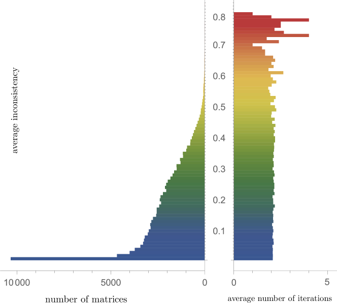
While the relationship between the number of alternatives and the number of iterations of the algorithms seems significant, there is no evident relationship between the inconsistency of the tested matrices and the number of iterations. In order to observe this possible relationship, we divided the set of tested matrices into subsets where the first one contained C matrices with CI(C) between 0 and $0.01$, the second one between $0.01$ and $0.02$, and so on. For each interval, we counted the average inconsistency, the average number of iterations and the set count. As long as the set size did not fall below a few tens of elements, the average number of iterations remained similar regardless of the average inconsistency of the matrix in a given subset (Fig. 2). Since the result was similar in each of the four variants considered in the figure, we used in (Fig. 2) the result for the bubble algorithm and the LBR strategy. It is worth noting that the modifications made by the algorithm to the matrix do not change its level of inconsistency. Thus, attempts to detect such manipulation using only inconsistency measurements may be ineffective.

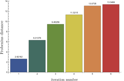
The Frobenius distance between the input matrix and the matrices that are the output of successive algorithms’ iterations increases. This is because each iteration changes subsequent elements of the matrix, moving it away from the original matrix (Fig. 3). This behavior can be observed regardless of the type of algorithm and strategy adopted.

Figure 3: Frobenius distance between input matrix and its subsequent improvements. Average values for greedy algorithm and LBN strategy.

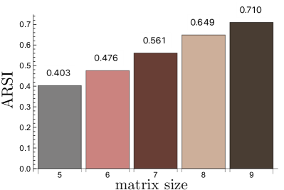
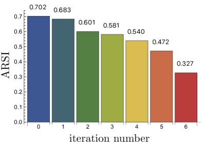
Similarly, a consistently observable pattern is the decline in the Average Ranking Stability Index ARSI values. The ARSI values depend on the size of the matrix i.e., the larger the dimension of the matrix, the higher the ARSI (Fig. 4).

Figure 4: The average RSI (ARSI) value for the matrices studied depending on the size of the matrix.

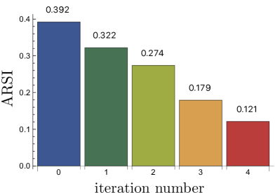
Therefore in the study we calculated the corresponding values in groups of matrices of the same dimensions (Fig. 5). This corresponds to the intuitive observation that making the first intervention is the most difficult. Each subsequent one comes more and more easily. More formally, ARSI is being reduced in subsequent iterations of the algorithm, since they make two alternatives’ weights equal and closer to the rest and leave other alternatives’ weights unchanged. This implies that each manipulation increases the possibility of other manipulations.

(a) PC matrices $5\times 5$

(b) PC matrices $9\times 9$

Figure 5: Decreasing (average) value of ARSI for modified matrices in successive iterations using the greedy algorithm and LBN strategy as an example. Iteration $0$ shows the average ARSI value for the unmodified input matrices.

5 Conclusions

In the presented work we have introduced two algorithms of promoting a given alternative to the position of a ranking leader. They are both based on the EQ algorithm equating two given alternatives in a ranking. The first one, called the greedy algorithm, in each step equates the rankings of a promoted alternative and the current leader. The second one (the bubble algorithm) in each step equates an alternative with the one directly preceding it in the ranking. We have also defined the Average Ranking Stability Index (ARSI) for a PC matrix to measure how easily the data manipulation may happen.

The Monte Carlo study has shown that in general it is harder to create a new leader when there are more alternatives. On the other hand, the input inconsistency of data has no influence on the ease of manipulation. The third conclusion is that each each manipulation facilitates the subsequent ones. The final remark is that the EQ algorithm does not change the scale, i.e. if the input PC matrix elements have been taken from the range $[-M,M]$, the output matrix elements had the same property.

6 Acknowledgments

The research has been supported by The National Science Centre, Poland, project no. 2021/41/B/HS4/03475 and by the Polish Ministry of Science and Higher Education (task no. 11.11.420.004).

References

- [1] C.A. Bana e Costa, De Corte, J.M., and J.C. Vansnick. On the mathematical foundation of MACBETH. In J. Figueira, S. Greco, and M. Ehrgott, editors, Multiple Criteria Decision Analysis: State of the Art Surveys, pages 421–463. Springer Verlag, Boston, Dordrecht, London, 2016.
- [2] J. Barzilai. Consistency measures for pairwise comparison matrices. Journal of Multi-Criteria Decision Analysis, 7(3):123–132, 1998.
- [3] J. Barzilai and B. Golany. Deriving weights from pairwise comparison matrices: The additive case. Operations Research Letters, 9(6):407–410, November 1990.
- [4] J. Benítez, W. W. Koczkodaj, and A. Kowalczyk. Computationally efficient orthogonalization for pairwise comparisons method. Applied Mathematics and Computation, 473:128651, July 2024.
- [5] F. Brandt, V. Conitzer, U. Endriss, J. Lang, and A. D. Procaccia, editors. Handbook of Computational Social Choice. Cambridge University Press, March 2016.
- [6] J.P. Brans and B. Mareschal. PROMETHEE methods. In J. Figueira, S. Greco, and M. Ehrgott, editors, Multiple Criteria Decision Analysis: State of the Art Surveys, pages 187–219. Springer Verlag, Boston, Dordrecht, London, 2016.
- [7] M. Brunelli. A survey of inconsistency indices for pairwise comparisons. International Journal of General Systems, 47(8):751–771, September 2018.
- [8] B. Cavallo, J. Mazurek, and J. Ramík. A comparative study on precision of pairwise comparison matrices. Fuzzy Optimization and Decision Making, November 2023.
- [9] G. B. Crawford. The geometric mean procedure for estimating the scale of a judgement matrix. Mathematical Modelling, 9(3–5):327 – 334, 1987.
- [10] L. Csató and D. G. Petróczy. On the monotonicity of the eigenvector method. European Journal of Operational Research, 2020.
- [11] Y. Dong, Y. Liu, H. Liang, F. Chiclana, and E. Herrera-Viedma. Strategic weight manipulation in multiple attribute decision making. Omega, 75:154–164, 2018.
- [12] Y. Dong, Q. Zha, H. Zhang, and F. Herrera. Consensus Reaching and Strategic Manipulation in Group Decision Making With Trust Relationships. IEEE Transactions on Systems, Man, and Cybernetics: Systems, 51(10):6304–6318, October 2021.
- [13] P. Faliszewski, E. Hemaspaandra, and L. A. Hemaspaandra. Using complexity to protect elections. Communications of the ACM, 53(11):74–82, 2010.
- [14] M. Fedrizzi, M. Brunelli, and A. Caprila. The linear algebra of pairwise comparisons. International Journal of Approximate Reasoning, 118:190–207, March 2020.
- [15] A. Gibbard. Manipulation of voting schemes: A general result. Econometrica, 41(4):587–601, 1973. ISBN: 00129682.
- [16] P. T. Kazibudzki. On estimation of priority vectors derived from inconsistent pairwise comparison matrices. Journal of Applied Mathematics and Computational Mechanics, 21(4):52–59, 2022.
- [17] W. W. Koczkodaj, R. Smarzewski, and J. Szybowski. On Orthogonal Projections on the Space of Consistent Pairwise Comparisons Matrices. Fundamenta Informaticae, 172(4):379–397, 2020. Publisher: IOS Press.
- [18] W. W. Koczkodaj and R. Urban. Axiomatization of inconsistency indicators for pairwise comparisons. International Journal of Approximate Reasoning, 94:18–29, March 2018.
- [19] K. Kułakowski. On the properties of the priority deriving procedure in the pairwise comparisons method. Fundamenta Informaticae, 139(4):403 – 419, July 2015.
- [20] K. Kułakowski, J. Mazurek, and M. Strada. On the similarity between ranking vectors in the pairwise comparison method. Journal of the Operational Research Society, 0(0):1–10, 2021.
- [21] K. Kułakowski, J. Szybowski, J. Mazurek, and S. Ernst. Resilient heuristic aggregation of judgments in the pairwise comparisons method. Information Sciences, 657:119979, 2024.
- [22] K. Kułakowski, J. Szybowski, and A. Prusak. Towards quantification of incompleteness in the pairwise comparisons methods. International Journal of Approximate Reasoning, 115:221–234, October 2019.
- [23] O. Lev and Y. Lewenberg. “Reverse Gerrymandering”: Manipulation in Multi-Group Decision Making. Proceedings of the AAAI Conference on Artificial Intelligence, 33(01):2069–2076, July 2019.
- [24] X. Liang, J. Guo, and P. Liu. A consensus model considers managing manipulative and overconfident behaviours in large-scale group decision-making. Information Sciences, 654:119848, January 2024.
- [25] J. Mazurek. Advances in Pairwise Comparisons: Detection, Evaluation and Reduction of Inconsistency. Multiple Criteria Decision Making. Springer Nature Switzerland, 2023.
- [26] J. Rezaei. Best-worst multi-criteria decision-making method. Omega, 53(C):49–57, June 2015.
- [27] T. L. Saaty. A scaling method for priorities in hierarchical structures. Journal of Mathematical Psychology, 15(3):234 – 281, 1977.
- [28] Y. Sasaki. Strategic manipulation in group decisions with pairwise comparisons: A game theoretical perspective. European Journal of Operational Research, 304(3):1133–1139, February 2023.
- [29] Q. Sun, J. Wu, F. Chiclana, S. Wang, E. Herrera-Viedma, and R. R. Yager. An approach to prevent weight manipulation by minimum adjustment and maximum entropy method in social network group decision making. Artificial Intelligence Review, December 2022.
- [30] J. Szybowski, K. Kułakowski, and S. Ernst. Almost optimal manipulation of a pair of alternatives, 2023.
- [31] J. Wu, M. Cao, F. Chiclana, Y. Dong, and E. Herrera-Viedma. An Optimal Feedback Model to Prevent Manipulation Behavior in Consensus Under Social Network Group Decision Making. IEEE Transactions on Fuzzy Systems, 29(7):1750–1763, July 2021.
- [32] R. R. Yager. Penalizing strategic preference manipulation in multi-agent decision making. IEEE Transactions on Fuzzy Systems, 9(3):393–403, 2001.
- [33] R. R. Yager. Defending against strategic manipulation in uninorm-based multi-agent decision making. European Journal of Operational Research, 141(1):217–232, 2002.