A Markov approach to credit rating migration
conditional on economic states

Michael Kalkbrener**footnotemark: *,   Natalie Packhamfootnotemark:
Abstract

We develop a model for credit rating migration that accounts for the impact of economic state fluctuations on default probabilities. The joint process for the economic state and the rating is modelled as a time-homogeneous Markov chain. While the rating process itself possesses the Markov property only under restrictive conditions, methods from Markov theory can be used to derive the rating process’ asymptotic behaviour. We use the mathematical framework to formalise and analyse different rating philosophies, such as point-in-time (PIT) and through-the-cycle (TTC) ratings. Furthermore, we introduce stochastic orders on the bivariate process’ transition matrix to establish a consistent notion of “better” and “worse” ratings. Finally, the construction of PIT and TTC ratings is illustrated on a Merton-type firm-value process.

Keywords: Risk management, credit risk, credit ratings, Markov chains

MSC classification: 60J20, 91G40, 60J05, 60E1511footnotetext: Michael Kalkbrener, Deutsche Bank AG, Otto-Suhr-Allee 16, 10585 Berlin, Germany.

22footnotetext: Natalie Packham, Berlin School of Economics and Law, Badensche Str. 52, 10825 Berlin, Germany.   Email: packham@hwr-berlin.de The views expressed in this paper are those of the authors and do not necessarily reflect the position of Deutsche Bank AG.

1 Introduction

It is generally accepted that corporate default rates depend on economic conditions (Wilson, 1998; Nickell et al., 2000; Bangia et al., 2002; Heitfield, 2005; Malik and Thomas, 2012). Rating systems, which are designed to provide information on the credit quality of corporates, differ with respect to the type of economic information reflected in the rating. The two main rating philosophies are through-the-cycle (TTC) ratings, which are insensitive to economic conditions and focus on company-specific criteria, and point-in-time (PIT) ratings, which reflect the current economic situation as well as expectations of future economic developments. However, no precise definition of PIT and TTC characteristics of rating systems has been established. One objective of this paper is to develop a mathematical framework for rating migration processes, factoring in the economic situation, that allows for a formal characterisation of PIT and TTC ratings.

The distinction between PIT and TTC rating concepts is particularly relevant for banks who need to comply with accounting standards and capital regulation. Assessing the credit risk of a company solely by its probability of default (PD), incentivises procyclical adjustments of financial institutions’ capital requirements, i.e., decreasing default rates in economic upturns would allow financial institutions to reduce capital for their corporate credit portfolios, while increasing default rates in economic downturns would increase capital requirements, see e.g. Borio et al. (2001); Behn et al. (2016) and references therein. As this procyclical capitalisation poses a threat to financial stability, financial regulators prefer banks to assess regulatory capital requirements for credit risk using TTC ratings and default probabilities,333Capital requirements regulation and directive – CRR/CRD IV, Article 502 which are designed to be stable through the business cycle. In contrast, the International Financial Reporting Standard (IFRS) 9 as well as the accounting standard Current Expected Credit Losses (CECL) require financial institutions to calculate expected credit losses that reflect current economic conditions and forecasts of future economic conditions,444International Financial Reporting Standard (IFRS) 9, Paragraph 5.5.17. For CECL, see FASB Accounting Standards Update (ASU) 2016-13. leading to the challenging problem of incorporating the impact of economic factors into the estimation of default probabilities.

Models of rating migration processes specified as time-homogeneous Markov chains, as is common in the credit risk literature (Duffie and Singleton, 2003; Jarrow et al., 1997; Lando, 2004; Bluhm et al., 2003), lack the necessary flexibility to capture the complex link to the macroeconomic environment. To resolve this problem, several extensions of the simple Markov framework have been proposed in the literature: regime-switching models specify different rating migration matrices for periods of economic contraction and expansion (Bangia et al., 2002), mixtures of Markov chain models define rating migration processes as a combination of several Markov chains (Frydman and Schuermann, 2008; Fei et al., 2012).

The model presented in this paper extends the above-mentioned approaches by incorporating an economic state process with finitely many states. Our starting point is to model the evolution of economic states $\mathcal{A}$ as a time-homogeneous Markov chain $(A_{t})_{t\in\mathbb{N}_{0}}$. Rating migrations $(R_{t})_{t\in\mathbb{N}_{0}}$, specified on the state space of rating classes $\mathcal{R}$, are not assumed to follow a Markov process but are defined by transition matrices that depend on the state of the economy. However, it is a key assumption that the rating process has the Markov property if its state space is extended to the product space $\mathcal{A}\times\mathcal{R}$ consisting of economic states and rating classes. More formally, the combined process $(X_{t})_{t\in\mathbb{N}_{0}}=(A_{t},R_{t})_{t\in\mathbb{N}_{0}}$ defined on the product space $\mathcal{A}\times\mathcal{R}$ of economic states and ratings is assumed to be a time-homogeneous Markov chain.

In the first part of the paper (Sections 24), we study conditions on the conditional transition matrices that guarantee the Markov property for $(R_{t})_{t\in\mathbb{N}_{0}}$ within the state space $\mathcal{R}$ itself. Since $(R_{t})_{t\in\mathbb{N}_{0}}$ is a projection of the time-homogeneous Markov chain $(X_{t})_{t\in\mathbb{N}_{0}}$, this problem is a special case of the more general question of whether functions of Markov chains possess the Markov property (Rosenblatt, 1971). We show that only a small subclass of TTC rating migration processes are (time-inhomogeneous) Markov chains on the state space $\mathcal{R}$, which provides theoretical support to the claim that real-world rating systems do not have the Markov property, e.g. Altman (1998); Lando and Skødeberg (2002); Güttler and Raupach (2010). However, it can be shown that for any non-Markovian rating process $(R_{t})_{t\in\mathbb{N}_{0}}$ there exists a time-inhomogeneous Markov chain $({\widetilde{R}}_{t})_{t\in\mathbb{N}_{0}}$on $\mathcal{R}$ with time-dependent transition matrices $({\widetilde{P}}_{t})_{t\in{\mathbb{N}}}$ that has identical default rates and future rating distributions as $(R_{t})_{t\in\mathbb{N}_{0}}$, i.e.,

$${\mathbb{P}}({\widetilde{R}}_{t}=r)={\mathbb{P}}(R_{t}=r),\quad t\in\mathbb{N}_{0},\quad r\in{\mathcal{R}},$$

where ${\mathbb{P}}(R_{t}=r)$ denotes the probability of $R_{t}$ being in rating class $r$. Using the Perron-Frobenius Theorem, we prove that the sequence of transition matrices $({\widetilde{P}}_{t})_{t\in{\mathbb{N}}}$ converges to a limit, denoted by ${\widetilde{P}}_{\infty}$. The corresponding time-homogeneous Markov chain on $\mathcal{R}$ with transition matrix ${\widetilde{P}}_{\infty}$ replicates the rating distribution and default behaviour of $(R_{t})_{t\in\mathbb{N}_{0}}$ in the asymptotic limit. In particular, ${\widetilde{P}}_{\infty}$ specifies the vector of asymptotic default probabilities of the different rating classes.

The explicit incorporation of an economic state process into the specification of the rating process $(R_{t})_{t\in\mathbb{N}_{0}}$ allows for a unified analysis of different rating philosophies. In the second part of the paper (Section 5), we provide a formal definition of PIT and TTC rating migration processes based on a decomposition of conditional transition matrices into default and non-default components. In a nutshell, TTC ratings have a firm-specific character, i.e., the non-default rating transitions are insensitive to economic state fluctuations, whereas PIT non-default ratings are explicitly assigned according to a firm’s PD (probability of default), whence they swing with economic state fluctuations.

The third part of the paper (Section 6) is concerned with orderings on distributions on the state space $\mathcal{A}\times\mathcal{R}$ of the combined process $(X_{t})_{t\in\mathbb{N}_{0}}$, formalising the notions of “better” or “worse” economic states and rating states. A natural approach to order rating states is by first-order stochastic dominance, see Jarrow et al. (1997), which, amongst other properties, preserves the order of long-term default probabilities. Several extensions of first-order stochastic dominance exist in a multivariate setting, amongst which stochastic dominance and the upper orthant order turn out to be relevant for the combined process $(X_{t})_{t\in\mathbb{N}_{0}}$. We analyse conditions for stochastic monotonicity of transition matrices of $(X_{t})_{t\in\mathbb{N}_{0}}$ as well as conditions for preserving the order of multi-year default probabilities conditional on the initial economic state and rating.

In the fourth part (Section 7), we apply the theoretical framework to create PIT and TTC ratings using a Merton-type firm-value process (Merton, 1974). The economic state influences the firm-value by adding a systematic drift. PIT ratings are determined by classifying firms according to their PDs. While the PIT rating construction is relatively straightforward, there are various methods to build TTC ratings, such as considering a firm’s idiosyncratic risk or stressed PDs. In a worked example we select the TTC rating that most closely aligns with the PIT rating by minimising the differences in multi-year PDs conditional on various combinations of initial economic states and PIT ratings. This provides valuable insights into how PIT and TTC ratings coexist, as well as their similarities and differences.

We conclude by demonstrating how rating models within our framework concurrently meet requirements of ratings and PDs in both accounting and regulatory capital standards (Section 8).

2 Conditional rating transition matrices

2.1 Definition

We refer to Norris (1998) for basic definitions in the theory of Markov chains. Let $(\Omega,\mathcal{F},{\mathbb{P}})$ be a probability space. On this probability space there exists a stochastic process $(A_{t})_{t\in\mathbb{N}_{0}}$ taking values in a set $\mathcal{A}$, which consists of $K$ economic states. The economic state process is assumed to be a time-homogeneous Markov chain with transition matrix $M=(m_{ab})\in[0,1]^{K\times K}$, i.e., ${\mathbb{P}}(A_{t+1}=b|A_{t}=a)=m_{ab}$ for $t\in\mathbb{N}_{0}$.

In addition, a stochastic process $(R_{t})_{t\in\mathbb{N}_{0}}$ denoting the rating process of a firm exists, taking values in the set $\mathcal{R}$. The set $\mathcal{R}$ has $J$ elements, which are interpreted as rating states including an absorbing default state $\overline{r}$. The subset of non-default ratings is denoted by $\widehat{\mathcal{R}}$, i.e., $\widehat{\mathcal{R}}={\mathcal{R}}\setminus\{\overline{r}\}$.

We do not require the rating process $(R_{t})_{t\in\mathbb{N}_{0}}$ to have the Markov property. Instead we make the weaker assumption that the joint process $(X_{t})_{t\in\mathbb{N}_{0}}=(A_{t},R_{t})_{t\in\mathbb{N}_{0}}$ taking values in the product space $\mathcal{X}=\mathcal{A}\times\mathcal{R}$ is a time-homogeneous Markov chain with transition matrix

$$P=(p_{(a,r),(b,s)})\in[0,1]^{KJ\times KJ},$$ (1)

where

$$p_{(a,r),(b,s)}={\mathbb{P}}(A_{t+1}=b,R_{t+1}=s|A_{t}=a,R_{t}=r)$$

denotes the probability of moving from the state $(a,r)$ to $(b,s)$. The distribution of $X_{0}$ is denoted by $\lambda\in[0,1]^{KJ}$. W.l.o.g. we assume a default probability of 0 at time 0, i.e., $\lambda_{(a,\overline{r})}=0$ for $a\in{\mathcal{A}}$.

It is a reasonable assumption that if the current economic state is known, knowledge about the current rating does not add information about the future economic state. The following Lemma establishes that, under this assumption, the transition matrix $P$ is fully determined by

  1. 1.

    the transition probabilities $m_{ab}$ of the economic state process and

  2. 2.

    the rating transition probabilities conditional on economic state transitions, i.e., the conditional probabilities ${\mathbb{P}}(R_{t+1}=s|R_{t}=r,A_{t+1}=b,A_{t}=a)$.

To formalize this statement, conditional rating migration matrices $M^{(a,b)}=(m_{rs}^{(a,b)})\in[0,1]^{J\times J}$ are defined for each economic state transition $(a,b)\in{\mathcal{A}}\times{\mathcal{A}}$, where

$$m_{rs}^{(a,b)}={\mathbb{P}}(R_{t+1}=s|R_{t}=r,A_{t+1}=b,A_{t}=a).$$

We assume that migrations from non-default ratings to any other rating class have positive probability, i.e., $m_{rs}^{(a,b)}>0$ for all $r\in\widehat{\mathcal{R}}$, $s\in{\mathcal{R}}$ and $a,b\in\mathcal{A}$. Since $\overline{r}$ is absorbing, $m_{\overline{r}r}^{(a,b)}=0$ and $m_{\overline{r}\,\overline{r}}^{(a,b)}=1$.

Lemma 2.1.

$p_{(a,r),(b,s)}=m_{ab}m_{rs}^{(a,b)}$ if and only if $A_{t+1}$ and $R_{t}$ are conditionally independent given $A_{t}$.

Proof.

$\Leftarrow$”: Using that ${\mathbb{P}}(A_{t+1}=b|A_{t}=a)={\mathbb{P}}(A_{t+1}=b|A_{t}=a,R_{t}=r)$:

$\displaystyle m_{ab}m_{rs}^{(a,b)}$ $\displaystyle={\mathbb{P}}(A_{t+1}=b|A_{t}=a)\,{\mathbb{P}}(R_{t+1}=s|R_{t}=r,A_{t+1}=b,A_{t}=a)$
$\displaystyle={\mathbb{P}}(A_{t+1}=b|A_{t}=a,R_{t}=r)\,{\mathbb{P}}(R_{t+1}=s|R_{t}=r,A_{t+1}=b,A_{t}=a)$
$\displaystyle={\mathbb{P}}(A_{t+1}=b,R_{t+1}=s|R_{t}=r,A_{t}=a)$
$\displaystyle=p_{(a,r),(b,s)}.$

$\Rightarrow$” follows in the same way. ∎

From now on we assume that $A_{t+1}$ and $R_{t}$ are conditionally independent given $A_{t}$. It immediately follows from $P=(m_{ab}m_{rs}^{(a,b)})$ that the process $X_{t}$ as well as the rating process $R_{t}$, which can be considered as the projection of $X_{t}$ onto the state space ${\mathcal{R}}$, are completely specified by the initial distribution $\lambda\in[0,1]^{KJ}$ of $(A_{0},R_{0})$, the transition matrix $M\in[0,1]^{K\times K}$ of $A_{t}$ and the $K^{2}$ conditional rating migration matrices $M^{(a,b)}\in[0,1]^{J\times J}$. The probability of a path of economic states and ratings has the form

$${\mathbb{P}}(X_{0}=(a_{0},r_{0}),\ldots,X_{T}=(a_{T},r_{T}))={\mathbb{P}}(X_{0}=(a_{0},r_{0}))\prod_{t=0}^{T-1}m_{a_{t}a_{t+1}}m_{r_{t}r_{t+1}}^{(a_{t},a_{t+1})}.$$

2.2 Example of a rating system

The following example shows the economic state transition matrix $M$ and the $M^{(a,b)}$ and $P$ matrices of a rating system. It is derived from a Merton model (Merton (1974)), as will be explained in detail in Section 7.

Economic state transitions are assumed to follow a Markov process with transition matrix

$$M=\begin{pmatrix}0.8&0.175&0.025\\ 0.1&0.8&0.1\\ 0.025&0.175&0.8\end{pmatrix}.$$ (2)

Here, the first state is considered to be a good, the second state a neutral and the third state a bad economic state.

Refer to caption
Refer to caption
Figure 1: $M^{(a,b)}$ matrices (left) and $P$ matrix (right). Economic states are labelled 1 (good), 2 (neutral) and 3 (bad). Ratings are ordered from the highest rating class to the worst (default). Darker shades indicate values closer to one, whereas white indicates a value of zero or close to zero.

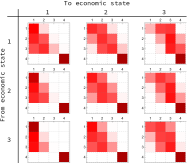
There are four rating classes, of which the first three – ordered from best to worst – are non-default ratings and the fourth is the (absorbing) default state. The left hand side of Figure 1 shows the $M^{(a,b)}$ matrices for economic states $a,b\in\{1,2,3\}$. In this example, the economic state transition $(a,b)$ has a strong impact on rating migration: if $b$ is the best economic state 1, upgrades clearly dominate downgrades (as illustrated by the three matrices in the first column), whereas a transition to the worst state $b=3$ increases the probability of downgrades. Two examples of $M^{(a,b)}$ matrices are:

$$M^{(2,1)}=\begin{pmatrix}0.9808&0.0192&0.0001&4\cdot 10^{-7}\\ 0.8371&0.1598&0.0030&0.0001\\ 0.6137&0.3660&0.0195&0.0008\\ 0&0&0&1\end{pmatrix},\ \ \ M^{(2,3)}=\begin{pmatrix}0.1737&0.5058&0.3188&0.0017\\ 0.0213&0.2460&0.7004&0.0323\\ 0.0033&0.0911&0.7814&0.1242\\ 0&0&0&1\end{pmatrix}.$$

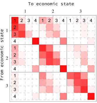
The right-hand side of Figure 1 shows the $P$ matrix resulting from $p_{(a,r),(b,s)}=m_{ab}m^{(a,b)}_{rs}$, for all $a,b\in\mathcal{A}$ and $r,s\in\mathcal{R}$.

3 Analysis of the Markov property of rating processes

3.1 A class of Markovian rating processes

As a consequence of the dependence on the underlying economic states, rating processes $(R_{t})_{t\in\mathbb{N}_{0}}$ typically do not have the Markov property if their state space is restricted to the set of rating classes. In this section, we establish conditions on the transition matrices $M^{(a,b)}$ that ensure that $(R_{t})_{t\in\mathbb{N}_{0}}$ is a Markov process on $\mathcal{R}$.

It is a key model assumption in this paper that rating processes have the Markov property on the extended state space $\mathcal{X}=\mathcal{A}\times\mathcal{R}$, which consists of all combinations of economic states and rating classes. More formally, $(R_{t})_{t\in\mathbb{N}_{0}}$ is the projection of the time-homogeneous Markov chain $(X_{t})_{t\in\mathbb{N}_{0}}$ with state space $\mathcal{X}$ onto the state space $\mathcal{R}$. Hence, the question whether $(R_{t})_{t\in\mathbb{N}_{0}}$ is a Markov process can be addressed in the more general context of studying the Markov property of functions of Markov processes, see Rosenblatt (1971).

The general results in Rosenblatt (1971) can be significantly improved in our setup by utilizing the structure of the transition matrix $P=(p_{(a,r),(b,s)})\in[0,1]^{KJ\times KJ}$ given in Lemma 2.1, i.e., representing $p_{(a,r),(b,s)}$ in the form $p_{(a,r),(b,s)}=m_{ab}m_{rs}^{(a,b)}$. Not surprisingly, severe restrictions on the conditional transition matrices $M^{(a,b)}$ are required to ensure the Markov property of the rating process $(R_{t})_{t\in\mathbb{N}_{0}}$. It turns out that the following definition formalizes the key property of conditional transition matrices $M^{(a,b)}$ of Markovian rating processes $(R_{t})_{t\in\mathbb{N}_{0}}$.

Definition 3.1.

The conditional transition matrices $M^{(a,b)}$ have identical ratios of non-default migration probabilities if for all $r,r^{\prime},s,s^{\prime}\in\widehat{\mathcal{R}}$ and $a,a^{\prime},b,b^{\prime}\in\mathcal{A}$

$$\frac{m_{rs}^{(a,b)}}{m_{r^{\prime}s^{\prime}}^{(a,b)}}=\frac{m_{rs}^{(a^{\prime},b^{\prime})}}{m_{r^{\prime}s^{\prime}}^{(a^{\prime},b^{\prime})}}.$$ (3)

It is easily verified that the two matrices provided in the example in Section 2.2 do not fulfil this: $m_{1,1}^{(2,1)}/m_{1,2}^{(2,1)}>1$, while $m_{1,1}^{(2,3)}/m_{1,2}^{(2,3)}<1$.

As an example of a simple class of rating migration processes that have identical ratios of non-default migration probabilities, consider processes based on just two ratings $r$ and $\overline{r}$. Since $r$ is the only element of $\widehat{\mathcal{R}}$ condition (3) is always satisfied, regardless of the specification of the conditional transition matrices.

The above condition significantly reduces the free parameters that are required for specifying conditional transition matrices. Choose $a,b\in{\mathcal{A}}$ and $r,s\in\widehat{\mathcal{R}}$ and specify $M^{(a,b)}$ and $m_{rs}^{(a^{\prime},b^{\prime})}$ for all $(a^{\prime},b^{\prime})\not=(a,b)$. All other parameters $m_{r^{\prime}s^{\prime}}^{(a^{\prime},b^{\prime})}$ are defined by (3), i.e., for $(r^{\prime},s^{\prime})\not=(r,s)$

$$m_{r^{\prime}s^{\prime}}^{(a^{\prime},b^{\prime})}=\frac{m_{r^{\prime}s^{\prime}}^{(a,b)}}{m_{rs}^{(a,b)}}m_{rs}^{(a^{\prime},b^{\prime})}.$$

Since $M^{(a,b)}$ is a stochastic matrix with one absorbing state, only $(J-1)^{2}+K^{2}-1$ free parameters are required for fully specifying conditional transition matrices with identical ratios of non-default migration probabilities. In the case $K=1$, just one rating transition matrix is defined, which is equivalent to the standard specification of a time-homogeneous Markov chain. For $K>1$, the number of conditional rating migration matrices $M^{(a,b)}$ as well as the number of free parameters increases by $K^{2}$.

The set of Equations (3) is a sufficient condition for the Markov property, see Corollary 3.3. In fact, Theorem 3.2 shows that the Equations (3) are equivalent to the economic state variable $A_{t}$ being independent of the rating history up to time $t$ (conditional on no default), which is a slightly stronger condition than the Markov property of $(R_{t})_{t\in\mathbb{N}_{0}}$.

More formally, let $t\in\mathbb{N}_{0}$. Conditional on no default, the economic state variable $A_{t}$ is independent of the rating history up to time $t$ if for all $a\in\mathcal{A}$ and $r_{0},s_{0},\ldots,r_{t},s_{t}\in\widehat{\mathcal{R}}$ with ${\mathbb{P}}(R_{0}=r_{0},\ldots,R_{t}=r_{t})>0$ and ${\mathbb{P}}(R_{0}=s_{0},\ldots,R_{t}=s_{t})>0$,

$${\mathbb{P}}(A_{t}=a|R_{0}=r_{0},\ldots,R_{t}=r_{t})={\mathbb{P}}(A_{t}=a|R_{0}=s_{0},\ldots,R_{t}=s_{t})={\mathbb{P}}(A_{t}=a|R_{t}\not=\overline{r}).$$ (4)
Theorem 3.2.

The following conditions are equivalent.

  1. (i)

    The conditional transition matrices $M^{(a,b)}$ have identical ratios of non-default migration probabilities.

  2. (ii)

    For every joint distribution $\lambda\in[0,1]^{KJ}$ of independent variables $A_{0}$ and $R_{0}$ and every stochastic matrix $M\in[0,1]^{K\times K}$ the rating process $R_{t}$ specified by the distribution $\lambda$ and transition matrices $M$ and $M^{(a,b)}$ satisfies (4) for every $t\in\mathbb{N}_{0}$.

Proof.

In this proof we abbreviate a rating path $\{R_{0}=r_{0},\ldots,R_{t}=r_{t}\}$ and a path $\{A_{0}=a_{0},\ldots,A_{t}=a_{t}\}$ of economic states by $r_{0..t}$ and $a_{0..t}$ respectively.

$\Rightarrow$”: For $t\in\mathbb{N}_{0}$ let $a_{0},b_{0},\ldots,a_{t},b_{t}\in\mathcal{A}$, $r_{0},s_{0},\ldots,r_{t},s_{t}\in\widehat{\mathcal{R}}$ with ${\mathbb{P}}(a_{0..t})>0$ and ${\mathbb{P}}(b_{0..t})>0$. We assume that $A_{0}$ and $R_{0}$ are independent variables and ${\mathbb{P}}(R_{0}=r_{0})>0$ and ${\mathbb{P}}(R_{0}=s_{0})>0$. We first prove by induction on $t$ that

$$\frac{{\mathbb{P}}(r_{0..t}|a_{0..t})}{{\mathbb{P}}(s_{0..t}|a_{0..t})}=\frac{{\mathbb{P}}(r_{0..t}|b_{0..t})}{{\mathbb{P}}(s_{0..t}|b_{0..t})}.$$ (5)

Since $A_{0}$ and $R_{0}$ are independent, Equation (5) holds for $t=0$. For $t>0$, we assume that (5) holds for $t-1$. Note that

$${\mathbb{P}}(r_{0..t}|a_{0..t})=\frac{{\mathbb{P}}(r_{0..t-1},a_{0..t-1})m_{a_{t-1}a_{t}}m_{r_{t-1}r_{t}}^{(a_{t-1},a_{t})}}{{\mathbb{P}}(a_{0..t-1})m_{a_{t-1}a_{t}}}={\mathbb{P}}(r_{0..t-1}|a_{0..t-1})m_{r_{t-1}r_{t}}^{(a_{t-1},a_{t})}.$$ (6)

Hence, by induction and (3),

$$\frac{{\mathbb{P}}(r_{0..t}|a_{0..t})}{{\mathbb{P}}(s_{0..t}|a_{0..t})}=\frac{{\mathbb{P}}(r_{0..t-1}|a_{0..t-1})m_{r_{t-1}r_{t}}^{(a_{t-1},a_{t})}}{{\mathbb{P}}(s_{0..t-1}|a_{0..t-1})m_{s_{t-1}s_{t}}^{(a_{t-1},a_{t})}}=\\ \frac{{\mathbb{P}}(r_{0..t-1}|b_{0..t-1})m_{r_{t-1}r_{t}}^{(b_{t-1},b_{t})}}{{\mathbb{P}}(s_{0..t-1}|b_{0..t-1})m_{s_{t-1}s_{t}}^{(b_{t-1},b_{t})}}=\frac{{\mathbb{P}}(r_{0..t}|b_{0..t})}{{\mathbb{P}}(s_{0..t}|b_{0..t})}.$$

For proving (4) we apply Bayes formula. For $t=0$, Equation (4) is implied by the independence of $A_{0}$ and $R_{0}$. Otherwise it follows from (6) that Bayes formula can be expressed as

$${\mathbb{P}}(a_{0..t}|r_{0..t})=\frac{{\mathbb{P}}(a_{0..t}){\mathbb{P}}(r_{0..t-1}|a_{0..t-1})m_{r_{t-1}r_{t}}^{(a_{t-1},a_{t})}}{\sum_{(b_{0},\ldots,b_{t})\in{\mathcal{A}}^{t+1}}{\mathbb{P}}(b_{0..t}){\mathbb{P}}(r_{0..t-1}|b_{0..t-1})m_{r_{t-1}r_{t}}^{(b_{t-1},b_{t})}}.$$ (7)

Hence, ${\mathbb{P}}(a_{0..t}|r_{0..t})={\mathbb{P}}(a_{0..t}|s_{0..t})$ is equivalent to

$$\sum_{(b_{0},\ldots,b_{t})\in{\mathcal{A}}^{t+1}}{\mathbb{P}}(b_{0..t}){\mathbb{P}}(r_{0..t-1}|a_{0..t-1}){\mathbb{P}}(s_{0..t-1}|b_{0..t-1})m_{r_{t-1}r_{t}}^{(a_{t-1},a_{t})}m_{s_{t-1}s_{t}}^{(b_{t-1},b_{t})}=\\ \sum_{(b_{0},\ldots,b_{t})\in{\mathcal{A}}^{t+1}}{\mathbb{P}}(b_{0..t}){\mathbb{P}}(r_{0..t-1}|b_{0..t-1}){\mathbb{P}}(s_{0..t-1}|a_{0..t-1})m_{s_{t-1}s_{t}}^{(a_{t-1},a_{t})}m_{r_{t-1}r_{t}}^{(b_{t-1},b_{t})}.$$ (8)

By (5), Equation (8) holds if and only if

$$\sum_{(b_{0},\ldots,b_{t})\in{\mathcal{A}}^{t+1}}{\mathbb{P}}(b_{0..t}){\mathbb{P}}(r_{0..t-1}|a_{0..t-1}){\mathbb{P}}(s_{0..t-1}|b_{0..t-1})(m_{r_{t-1}r_{t}}^{(a_{t-1},a_{t})}m_{s_{t-1}s_{t}}^{(b_{t-1},b_{t})}-m_{s_{t-1}s_{t}}^{(a_{t-1},a_{t})}m_{r_{t-1}r_{t}}^{(b_{t-1},b_{t})})=0.$$

Since the conditional transition matrices $M^{(a,b)}$ have identical ratios of non-default migration probabilities it follows that $m_{r_{t-1}r_{t}}^{(a_{t-1},a_{t})}m_{s_{t-1}s_{t}}^{(b_{t-1},b_{t})}-m_{s_{t-1}s_{t}}^{(a_{t-1},a_{t})}m_{r_{t-1}r_{t}}^{(b_{t-1},b_{t})}=0$. Hence, we obtain ${\mathbb{P}}(a_{0..t}|r_{0..t})={\mathbb{P}}(a_{0..t}|s_{0..t})$, which implies (4).

$\Leftarrow$”: Let $a,a^{\prime},b,b^{\prime}\in\mathcal{A}$ and $r,r^{\prime},s,s^{\prime}\in\widehat{\mathcal{R}}$ such that $m_{rs}^{(a,b)}m_{r^{\prime}s^{\prime}}^{(a^{\prime},b^{\prime})}\not=m_{r^{\prime}s^{\prime}}^{(a,b)}m_{rs}^{(a^{\prime},b^{\prime})}$. If $b=b^{\prime}$ we choose $c\in\mathcal{A}$ with $c\not=b$. Obviously, at least one of the two inequalities

$$\frac{m_{rs}^{(a,b)}}{m_{r^{\prime}s^{\prime}}^{(a,b)}}\not=\frac{m_{rs}^{(a,c)}}{m_{r^{\prime}s^{\prime}}^{(a,c)}},\ \ \ \ \ \ \frac{m_{rs}^{(a^{\prime},b^{\prime})}}{m_{r^{\prime}s^{\prime}}^{(a^{\prime},b^{\prime})}}\not=\frac{m_{rs}^{(a,c)}}{m_{r^{\prime}s^{\prime}}^{(a,c)}}$$

holds. Hence, we can assume that $b\not=b^{\prime}$. We now define $A_{0}$ and $R_{0}$ as independent variables specified by

$${\mathbb{P}}(A_{0}=a)={\mathbb{P}}(A_{0}=a^{\prime})=\frac{1}{|\{a,a^{\prime}\}|},\ \ \ {\mathbb{P}}(R_{0}=r)={\mathbb{P}}(R_{0}=r^{\prime})=\frac{1}{|\{r,r^{\prime}\}|}.$$

Furthermore, it is assumed that the transition matrix $M$ satisfies $m_{ab}=m_{a^{\prime}b^{\prime}}=1/2$ if $a=a^{\prime}$ and $m_{ab}=m_{a^{\prime}b^{\prime}}=1$ if $a\not=a^{\prime}$.

In both cases, ${\mathbb{P}}(A_{0}=a,A_{1}=b)={\mathbb{P}}(A_{0}=a^{\prime},A_{1}=b^{\prime})=1/2$ and Bayes formula (7) specializes to

$${\mathbb{P}}(A_{0}=a,A_{1}=b|R_{0}=r,R_{1}=s)=\frac{m_{rs}^{(a,b)}}{m_{rs}^{(a,b)}+m_{rs}^{(a^{\prime},b^{\prime})}}.$$

Since $m_{rs}^{(a,b)}(m_{r^{\prime}s^{\prime}}^{(a,b)}+m_{r^{\prime}s^{\prime}}^{(a^{\prime},b^{\prime})})\not=m_{r^{\prime}s^{\prime}}^{(a,b)}(m_{rs}^{(a,b)}+m_{rs}^{(a^{\prime},b^{\prime})})$ we obtain

$\displaystyle{\mathbb{P}}(A_{0}=a,A_{1}=b|R_{0}=r,R_{1}=s)$ $\displaystyle=$ $\displaystyle\frac{m_{rs}^{(a,b)}}{m_{rs}^{(a,b)}+m_{rs}^{(a^{\prime},b^{\prime})}}$
$\displaystyle\not=$ $\displaystyle\frac{m_{r^{\prime}s^{\prime}}^{(a,b)}}{m_{r^{\prime}s^{\prime}}^{(a,b)}+m_{r^{\prime}s^{\prime}}^{(a^{\prime},b^{\prime})}}$
$\displaystyle=$ $\displaystyle{\mathbb{P}}(A_{0}=a,A_{1}=b|R_{0}=r^{\prime},R_{1}=s^{\prime}).$

It follows from $b\not=b^{\prime}$ that ${\mathbb{P}}(A_{0}=a,A_{1}=b)={\mathbb{P}}(A_{1}=b)$ and therefore

$${\mathbb{P}}(A_{1}=b|R_{0}=r,R_{1}=s)\not={\mathbb{P}}(A_{1}=b|R_{0}=r^{\prime},R_{1}=s^{\prime}).$$

Hence, (4) does not hold. ∎

Corollary 3.3.

The rating process $R_{t}$ has the Markov property if

  1. (i)

    the variables $A_{0}$ and $R_{0}$, which are specified by their joint distribution $\lambda\in[0,1]^{KJ}$, are independent and

  2. (ii)

    the conditional transition matrices $M^{(a,b)}$ have identical ratios of non-default migration probabilities.

Proof.

By Theorem 3.2, Equation (4) holds for $t\in\mathbb{N}_{0}$, which implies

$${\mathbb{P}}(A_{t}=a|R_{0}=r_{0},\ldots,R_{t}=r_{t})={\mathbb{P}}(A_{t}=a|R_{t}=r_{t})$$

for $a\in\mathcal{A}$ and $r_{0},\ldots,r_{t}\in\widehat{\mathcal{R}}$ with ${\mathbb{P}}(R_{0}=r_{0},\ldots,R_{t}=r_{t})>0$. Hence, in case of no default at time $t$, i.e., $R_{t}\not=\overline{r}$, we obtain

$${\mathbb{P}}(R_{t+1}=r_{t+1}|R_{0}=r_{0},\ldots,R_{t}=r_{t})\\ \begin{aligned} &=\sum_{a,b\in\mathcal{A}}{\mathbb{P}}(R_{t+1}=r_{t+1},A_{t}=a,A_{t+1}=b|R_{0}=r_{0},\ldots,R_{t}=r_{t})\\ &=\sum_{a,b\in\mathcal{A}}{\mathbb{P}}(R_{t+1}=r_{t+1},A_{t+1}=b|A_{t}=a,R_{0}=r_{0},\ldots,R_{t}=r_{t})\,{\mathbb{P}}(A_{t}=a|R_{0}=r_{0},\ldots,R_{t}=r_{t})\\ &=\sum_{a,b\in\mathcal{A}}{\mathbb{P}}(R_{t+1}=r_{t+1},A_{t+1}=b|R_{t}=r_{t},A_{t}=a){\mathbb{P}}(A_{t}=a|R_{t}=r_{t})\\ &={\mathbb{P}}(R_{t+1}=r_{t+1}|R_{t}=r_{t}).\end{aligned}$$

If $R_{t}=\overline{r}$ then the Markov property holds because $\overline{r}$ is absorbing. ∎

3.2 Time-inhomogeneous Markov chains on ratings

As shown above, rating processes typically do not have the Markov property. However, it is easy to prove that for each rating process $(R_{t})_{t\in\mathbb{N}_{0}}$, a time-inhomogeneous Markov process can be constructed that replicates the unconditional distribution of $(R_{t})_{t\in\mathbb{N}_{0}}$ for each $t\in\mathbb{N}_{0}$.555A Markov chain is time-inhomogeneous if the transition matrices are time-dependent, see e.g. Chapter 1 of Brémaud (1999). Using mathematical results from Markov chain theory, this process will then be used to determine the long-term and asymptotic rating transition behaviour of $(R_{t})_{t\in\mathbb{N}_{0}}$, see Section 4.

More precisely, we define a time-inhomogeneous Markov chain on the state space $\mathcal{R}$ that replicates the rating distribution

$$({\mathbb{P}}(R_{t}=r))_{r\in{\mathcal{R}}},\quad t\in\mathbb{N}_{0}.$$
Proposition 3.4.

There exists a time-inhomogeneous Markov process $({\widetilde{R}}_{t})_{t\in\mathbb{N}_{0}}$ with

  1. (i)

    state space $\mathcal{R}$,

  2. (ii)

    initial distribution ${\tilde{\lambda}}$ on $[0,1]^{J}$ defined by ${\tilde{\lambda}}=({\mathbb{P}}(R_{0}=r))_{r\in{\mathcal{R}}}$,

  3. (iii)

    transition matrices $({\widetilde{P}}_{t})_{t\in\mathbb{N}_{0}}$ that can be determined from $(\lambda,P)$, such that

    $${\mathbb{P}}({\widetilde{R}}_{t}=r)={\mathbb{P}}(R_{t}=r),\quad t\in\mathbb{N}_{0},\quad r\in{\mathcal{R}}.$$ (9)

In particular, long-term default probabilities and distributions of non-default ratings can be immediately derived via

$$({\mathbb{P}}(R_{T}=r))_{r\in{\mathcal{R}}}={\tilde{\lambda}}\cdot\prod_{t=1}^{T}{\widetilde{P}}_{t},\quad T\in\mathbb{N}_{0}.$$ (10)

Essentially, the distributions of the process ${\widetilde{R}}$ are averaged with respect to the economic state transitions. Depending on the initial distribution $\lambda$ of $(X_{t})_{t\in\mathbb{N}_{0}}=(A_{t},R_{t})_{t\in\mathbb{N}_{0}}$, information about the initial economic state may enter the rating distributions, which creates the time-inhomogeneity in the transitions.

Proof.

First, we construct transition matrices $({\widetilde{P}}_{t})_{t\in\mathbb{N}_{0}}$. For $t\in\mathbb{N}_{0}$, let $\lambda_{t}\in[0,1]^{KJ}$ be the distribution of $X_{t}$, i.e., $\lambda_{t,(a,r)}={\mathbb{P}}(X_{t}=(a,r))$ for $(a,r)\in\mathcal{X}$, and define the matrix ${\widetilde{P}}_{t}=({\tilde{p}}_{t,rs})\in[0,1]^{J\times J}$ for $t\geq 1$: if ${\mathbb{P}}(R_{t-1}=r)>0$, then

$\displaystyle{\tilde{p}}_{t,rs}$ $\displaystyle={\mathbb{P}}(R_{t}=s|R_{t-1}=r)=\sum_{a\in\mathcal{A}}{\mathbb{P}}(R_{t}=s|R_{t-1}=r,A_{t-1}=a)\cdot{\mathbb{P}}(A_{t-1}=a|R_{t-1}=r)$
$\displaystyle=\sum_{a\in\mathcal{A}}{\mathbb{P}}(R_{t}=s|R_{t-1}=r,A_{t-1}=a)\cdot\frac{{\mathbb{P}}(A_{t-1}=a,R_{t-1}=r)}{{\mathbb{P}}(R_{t-1}=r)}$
$\displaystyle=\frac{\sum_{a,b\in\mathcal{A}}p_{(a,r)(b,s)}\cdot\lambda_{t-1,(a,r)}}{\sum_{a^{\prime}\in\mathcal{A}}\lambda_{t-1,(a^{\prime},r)}}.$

Otherwise, ${\tilde{p}}_{t,rs}=0$ for $s\in\widehat{\mathcal{R}}$ and ${\tilde{p}}_{t,r\overline{r}}=1$. By definition, the matrices ${\widetilde{P}}_{t}$, $t\geq 1$, are stochastic and can be calculated iteratively from $(\lambda,P)$. Hence, the process $({\widetilde{R}}_{t})_{t\geq\mathbb{N}_{0}}$ can be defined as a time-inhomogeneous Markov chain. It is easily verified that ${\mathbb{P}}({\widetilde{R}}_{t}=r)={\mathbb{P}}(R_{t}=r)$, $t>0$: From

$${\mathbb{P}}(R_{t}=s)=\sum_{r\in{\mathcal{R}}}{\mathbb{P}}(R_{t}=s|R_{t-1}=r)\cdot{\mathbb{P}}(R_{t-1}=r),$$

the claim follows by definition of ${\tilde{\lambda}}$ and by induction. ∎

Bluhm and Overbeck (2007) propose a parametric class of time-inhomogeneous Markov chains to calibrate observed multi-year default rates. Proposition 3.4 provides theoretical support to the claim that a convincing fit can be achieved even if the underlying process is not Markovian.

4 Asymptotic properties

In this section, we use standard techniques from the theory of Markov chains to prove that the sequence of transition matrices $({\widetilde{P}}_{t})_{t\in\mathbb{N}_{0}}$ converges to a limit, denoted by ${\widetilde{P}}_{\infty}$. The proof is based on the Perron-Frobenius Theorem (Perron (1907); Frobenius (1912)). In order to apply the theorem we assume in this section that the economic state process $(A_{t})_{t\in\mathbb{N}_{0}}$ is irreducible and aperiodic. Hence, the transition matrix $M$ is primitive, i.e., there exists an integer $k$ such that $M^{k}>0$. Furthermore, recall that $m^{(a,b)}_{rs}>0$ for all $r\in\widehat{\mathcal{R}}$, $s\in{\mathcal{R}}$ and $a,b\in\mathcal{A}$. This assumption implies that $\widehat{P}$ is a primitive matrix, where $\widehat{\mathcal{X}}=\mathcal{A}\times\widehat{\mathcal{R}}$ and $\widehat{P}$ is the restriction of $P$ to $\widehat{\mathcal{X}}$, i.e., $\widehat{P}=(\hat{p}_{(a,r),(b,s)})\in[0,1]^{K(J-1)\times K(J-1)}$ with $\hat{p}_{(a,r),(b,s)}=p_{(a,r),(b,s)}$ for $(a,r),(b,s)\in\widehat{\mathcal{X}}$. Likewise, we denote the restriction of $\lambda$ to $\widehat{\mathcal{X}}$ by $\hat{\lambda}\in[0,1]^{K(J-1)}$. Note that the assumption ${\mathbb{P}}(X_{0}\in\widehat{\mathcal{X}})=1$ implies that $\hat{\lambda}$ is a distribution on $\widehat{\mathcal{X}}$.

The matrix $\widehat{P}$ is not stochastic but it is primitive. Hence, the following properties are a consequence of the Perron-Frobenius Theorem (see e.g. Theorems 1.1 and 1.2 of Seneta (1973), Chapter 6 of Brémaud (1999)):

  1. (P1)

    The primitive matrix $\widehat{P}$ has a real eigenvalue $\rho$ with algebraic as well as geometric multiplicity one such that $\rho>0$ and $\rho>|\rho^{\prime}|$ for any other eigenvalue $\rho^{\prime}$. Moreover, the left eigenvector $\mu$ and the right eigenvector $\nu$ associated with $\rho$ can be chosen positive and such that $\mu\nu=1$.666Note that the left eigenvector $\mu$ is a row-vector and the right eigenvector $\nu$ is a column-vector, both of dimension $K(J-1)$. Hence, $\mu\nu$ is a real number whereas $\nu\mu$ is a $K(J-1)\times K(J-1)$ matrix.

  2. (P2)

    The matrix $((1/\rho)\widehat{P})^{n}$ converges to the matrix $\nu\mu$.

We assume that the components of $\mu$ add up to 1, i.e., $\mu$ is a distribution on $\widehat{\mathcal{X}}$. Let ${\tilde{\mu}}$ be the corresponding distribution on $\mathcal{R}$ specified by

$${\tilde{\mu}}_{r}=\sum_{a\in\mathcal{A}}\mu_{(a,r)}\text{ for }r\in\widehat{\mathcal{R}}\quad\text{ and }\quad{\tilde{\mu}}_{\overline{r}}=0,$$ (11)

and define the stochastic matrix ${\widetilde{P}}_{\infty}=({\tilde{p}}_{\infty,rs})\in[0,1]^{J\times J}$ by

$${\tilde{p}}_{\infty,rs}=\sum_{a\in\mathcal{A}}\mu_{(a,r)}\sum_{b\in\mathcal{A}}p_{(a,r),(b,s)}/{\tilde{\mu}}_{r},\quad r\in\widehat{\mathcal{R}},s\in{\mathcal{R}},$$ (12)

${\tilde{p}}_{\infty,\overline{r}r}=0$ for $r\in\widehat{\mathcal{R}}$ and ${\tilde{p}}_{\infty,\overline{r}\,\overline{r}}=1$.

We will now study the asymptotic properties of the Markov chain $(X_{t})_{t\in\mathbb{N}_{0}}$. Since ${\mathcal{A}}\times\{\overline{r}\}$ is a closed subset of the state space of $(X_{t})_{t\in\mathbb{N}_{0}}$ it immediately follows from the assumptions on the transition matrices $M$ and $M^{(a,b)}$ that

$$\lim_{t\rightarrow\infty}{\mathbb{P}}(X_{t}\in{\mathcal{A}}\times\{\overline{r}\})=1.$$

The more relevant question is the asymptotic behaviour of $(X_{t})_{t\in\mathbb{N}_{0}}$ conditionally on no default, which is summarized in the following theorem. In particular, it is shown that the conditional distribution of non-default rating states of $X$ converges to $\mu$, which implies convergence of $({\widetilde{P}}_{t})_{t\in{\mathbb{N}}}$ to ${\widetilde{P}}_{\infty}$. Furthermore, $1-\rho$ is the limit of the marginal default rates.777Marginal default rates refer to probabilities of default conditional on no prior default, as opposed to cumulative default rates.

In the following, note that $\{R_{t}=\overline{r}\}=\{X_{t}\in(\cdot,\overline{r})\}$ and $\{R_{t}\not=\overline{r}\}=\{X_{t}\not\in(\cdot,\overline{r})\}$. For ease of exposition, we use both notations.

Theorem 4.1.
  1. (i)

    For all $(a,r)\in\widehat{\mathcal{X}}$,

    $$\lim_{t\rightarrow\infty}{\mathbb{P}}(X_{t}=(a,r)|X_{t}\not\in(\cdot,\overline{r}))=\mu_{(a,r)}.$$

    Furthermore,

    $$\lim_{t\rightarrow\infty}{\widetilde{P}}_{t}={\widetilde{P}}_{\infty}\quad\text{ and }\quad\lim_{t\rightarrow\infty}{\mathbb{P}}(R_{t}=\overline{r}|R_{t-1}\not=\overline{r})=1-\rho.$$ (13)
  2. (ii)

    If the limit distribution $\mu=(\mu_{(a,r)})\in[0,1]^{K(J-1)}$ is the distribution of $X_{0}$ on the set of non-default states $\widehat{\mathcal{X}}$, i.e., $\hat{\lambda}=\mu$, then for all $t\in{\mathbb{N}}$

    $${\mathbb{P}}(X_{t}=(a,r)|X_{t}\notin(\cdot,\overline{r}))=\mu_{(a,r)}\quad\text{ and }\quad{\widetilde{P}}_{t}={\widetilde{P}}_{\infty}.$$
Proof.

(i) Since $\nu$ is a column-vector with positive entries and $\hat{\lambda}\not=0$ has only non-negative entries, the vector product $c=\hat{\lambda}\cdot\nu$ is a positive number. By (P2),

$$\lim_{t\rightarrow\infty}\hat{\lambda}\cdot((1/\rho)\widehat{P})^{t}=\hat{\lambda}\cdot\nu\cdot\mu=c\cdot\mu.$$ (14)

Let $t\in{\mathbb{N}}$ and define $\alpha_{t}\in[0,1]^{K(J-1)}$ as the distribution of $X_{t}$ conditional on $R_{t}\not=\overline{r}$, i.e.,

$$\alpha_{t}={\mathbb{P}}(X_{t}=(a,r)|X_{t}\not\in(\cdot,\overline{r}))_{(a,r)\in\widehat{\mathcal{X}}}.$$

Since the set of default states ${\mathcal{A}}\times\{\overline{r}\}$ is closed,

$$\alpha_{t}=\frac{{\mathbb{P}}(X_{t-1}\notin(\cdot,\overline{r}))}{{\mathbb{P}}(X_{t}\notin(\cdot,\overline{r}))}\cdot\alpha_{t-1}\cdot\widehat{P}=\frac{1}{{\mathbb{P}}(X_{t}\notin(\cdot,\overline{r}))}\cdot\hat{\lambda}\cdot\widehat{P}^{t}$$ (15)

and therefore

$$\alpha_{t}=\frac{\rho^{t}}{{\mathbb{P}}(X_{t}\notin(\cdot,\overline{r}))}\cdot\hat{\lambda}\cdot((1/\rho)\widehat{P})^{t}.$$

Using (14) and the fact that the $L_{1}$-norm of $\mu$ and $\alpha_{t}$ is 1 for each $t\in{\mathbb{N}}$ we obtain

$$\lim_{t\rightarrow\infty}\alpha_{t}=\mu.$$ (16)

Since $\widehat{P}$ is primitive, ${\mathbb{P}}(X_{t}=(a,r))>0$ for all $(a,r)\in\widehat{\mathcal{X}}$ and sufficiently large $t\in{\mathbb{N}}$. By the definition of the matrix ${\widetilde{P}}_{t}=({\tilde{p}}_{t,rs})\in[0,1]^{J\times J}$, for all $r\in\widehat{\mathcal{R}}$ and $s\in{\mathcal{R}}$

$\displaystyle{\tilde{p}}_{t+1,rs}$ $\displaystyle=\left(\sum_{a\in A}{\mathbb{P}}(X_{t}=(a,r))\sum_{b\in A}p_{(a,r),(b,s)}\right)/{\mathbb{P}}(X_{t}\in(\cdot,r))$
$\displaystyle=\left(\sum_{a\in A}({\mathbb{P}}(X_{t}=(a,r))/{\mathbb{P}}(X_{t}\notin(\cdot,\overline{r})))\sum_{b\in A}p_{(a,r),(b,s)}\right)/({\mathbb{P}}(X_{t}\in(\cdot,r))/{\mathbb{P}}(X_{t}\notin(\cdot,\overline{r})))$
$\displaystyle=\left(\sum_{a\in A}\alpha_{t,(a,r)}\sum_{b\in A}p_{(a,r),(b,s)}\right)/\sum_{a\in A}\alpha_{t,(a,r)}$ (17)

and ${\tilde{p}}_{t+1,\overline{r}r}=0$ for $r\in\widehat{\mathcal{R}}$ and ${\tilde{p}}_{t+1,\overline{r}\,\overline{r}}=1$. Hence, by (16),

$$\lim_{t\rightarrow\infty}{\widetilde{P}}_{t}={\widetilde{P}}_{\infty}.$$

From (16) and the first equation in (15) it follows that

$$\mu=\left(\lim_{t\rightarrow\infty}\frac{{\mathbb{P}}(X_{t-1}\notin(\cdot,\overline{r}))}{{\mathbb{P}}(X_{t}\notin(\cdot,\overline{r}))}\right)\cdot\mu\cdot\widehat{P}.$$

Since $\mu$ is an eigenvector with eigenvalue $\rho$,

$$\lim_{t\rightarrow\infty}\frac{{\mathbb{P}}(X_{t-1}\notin(\cdot,\overline{r}))}{{\mathbb{P}}(X_{t}\notin(\cdot,\overline{r}))}=\frac{1}{\rho}\quad\text{ and }\quad\lim_{t\rightarrow\infty}{\mathbb{P}}(X_{t}\in(\cdot,\overline{r})|X_{t-1}\notin(\cdot,\overline{r}))=1-\rho.$$

(ii) We now assume that $\hat{\lambda}=\mu$. It follows from (15) and $\mu\cdot\widehat{P}=\rho\cdot\mu$ that

$$\alpha_{t}=\frac{1}{{\mathbb{P}}(X_{t}\notin(\cdot,\overline{r}))}\cdot\mu\cdot\widehat{P}^{t}=\frac{1}{{\mathbb{P}}(X_{t}\notin(\cdot,\overline{r}))}\cdot\rho^{t}\cdot\mu=\mu$$

for every $t\in{\mathbb{N}}$ and therefore, by (17), ${\widetilde{P}}_{t}={\widetilde{P}}_{\infty}$. ∎

Definition 4.2.

Let $({S}_{t})_{t\in\mathbb{N}_{0}}$ be the time-homogeneous Markov chain with state space $\mathcal{R}$, transition matrix ${\widetilde{P}}_{\infty}=({\tilde{p}}_{rs})\in[0,1]^{J\times J}$ and initial distribution ${\tilde{\lambda}}$. Then $({S}_{t})_{t\in\mathbb{N}_{0}}$ is called the asymptotic approximation of $(R_{t})_{t\in\mathbb{N}_{0}}$.

The following corollary summarises the properties of the asymptotic approximation.

Corollary 4.3.
  1. (i)

    For any $r\in\widehat{\mathcal{R}}$,

    $$\lim_{t\rightarrow\infty}{\mathbb{P}}({S}_{t}=r|{S}_{t}\not=\overline{r})=\lim_{t\rightarrow\infty}{\mathbb{P}}(R_{t}=r|R_{t}\not=\overline{r}).$$ (18)
  2. (ii)

    If the limit distribution $\mu=(\mu_{(a,r)})\in[0,1]^{K(J-1)}$ is the distribution of $X_{0}$ on $\widehat{\mathcal{X}}$ then

    $${\mathbb{P}}({S}_{t}=r)={\mathbb{P}}(R_{t}=r)={\mathbb{P}}(X_{t}\in(\cdot,r))$$ (19)

    for $t\in\mathbb{N}_{0}$ and $r\in{\mathcal{R}}$. Furthermore, for $t\in{\mathbb{N}}$,

    $${\mathbb{P}}({S}_{t}=\overline{r}|{\mathbb{P}}({S}_{t-1}\not=\overline{r})={\mathbb{P}}(R_{t}=\overline{r}|{\mathbb{P}}({R}_{t-1}\not=\overline{r})=(1-\rho)\rho^{t-1}.$$ (20)
Proof.

We first assume that the limit distribution $\mu=(\mu_{(a,r)})\in[0,1]^{K(J-1)}$ is the distribution of $X_{0}$ on $\widehat{\mathcal{X}}$. It follows from Theorem 4.1 that ${\widetilde{R}}_{t\in\mathbb{N}_{0}}$ is a time-homogeneous Markov process, which equals the asymptotic approximation $({S}_{t})_{t\in\mathbb{N}_{0}}$, and

$${\mathbb{P}}(R_{t}\not=\overline{r}|R_{t-1}\not=\overline{r})=\rho\ \ \ \ \hbox{ and }\ \ \ \ {\mathbb{P}}(R_{t}=\overline{r}|R_{t-1}\not=\overline{r})=1-\rho$$

for all $t\in{\mathbb{N}}$. Hence, Equations (19) and (20) follow from Proposition 3.4. Furthermore, we obtain from Theorem 4.1 that $({\tilde{\mu}}_{r})_{r\in\widehat{\mathcal{R}}}$ is a positive left eigenvector of the restriction of ${\widetilde{P}}_{\infty}$ to $\widehat{\mathcal{R}}$. Analogously to the proof of Theorem 4.1, it follows from the Perron-Frobenius Theorem that

$$\lim_{t\rightarrow\infty}{\mathbb{P}}({S}_{t}=r|{S}_{t}\not=\overline{r})={\tilde{\mu}}_{r},\quad r\in\widehat{\mathcal{R}},$$ (21)

holds for any initial distribution of ${S}_{0}$. Hence, (18) follows from Theorem 4.1. ∎

5 Rating philosophies: Point-in-time and through-the-cycle

5.1 Definition of TTC and PIT ratings

This section deals with the characterisation of rating systems. Ratings are designed to provide information on the credit quality of an obligor. However, rating systems may differ with respect to the type of information reflected in the rating. There exist two main rating philosophies:

  1. (i)

    Point-in-time (PIT) ratings reflect the likelihood of default over a future period, e.g. one year, and are therefore dependent on firm-specific as well as systematic factors. The PIT rating of an obligor reflects the current state of the economy as well as all available information about the current and future economic development. As such, PIT ratings fluctuate over economic cycles (e.g. economic downturns lead to an increased number of downgrades), whereas expected one-period default probabilities of PIT rating classes are stable.

  2. (ii)

    In contrast, through-the-cycle (TTC) ratings have a longer rating horizon covering multiple periods, i.e., the rating is performed through the cycle. As a consequence, economic effects cancel out and TTC ratings are therefore independent of the state of the economy and, as such, are insensitive to economic or credit cycles. However, since actual corporate default rates depend on the economic environment the expected one-period default probabilities of TTC rating classes inevitably fluctuate with the economic cycle.888The characteristics of expected one-period default probabilities of TTC rating classes is different to TTC PDs defined in the literature as long-run averages of one-year default probabilities (e.g. Vallés (2006); Gordy and Howells (2004); Altman and Rijken (2004)) or stressed default probability (e.g. Heitfield (2005); Crouhy et al. (2001)). A comparison of these concepts in our mathematical framework is provided in Sections 7.3 and 8 of this paper.

Refer to caption
Figure 2: Example paths of economic states (top), PIT (middle) and TTC (bottom) rating distributions over 30 time periods for a firm starting in the best PIT rating. Economic states are ordered from best (1) to worst (3).

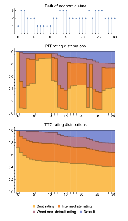
Figure 2 shows an example of an economic path (top) together with rating distributions of PIT and TTC ratings for a firm starting in the best PIT rating. This shows how PIT ratings fluctuate with the economy while TTC non-default ratings are insensitive to the economic environment. The rating models used in this illustration will be discussed in Section 7.

Both rating philosophies are interesting theoretical concepts. For practical applications, however, it is almost impossible to implement TTC or PIT ratings in a strict sense. First of all, it is very difficult to completely separate firm-specific components from macroeconomic developments. It is equally challenging to implement a rating system that comprehensively reflects the current state of the economy as well as all available information about the future economic development in a timely manner. As a consequence, real-world rating systems are typically hybrids in the following sense: Individual ratings are impacted by macroeconomic developments, e.g. upgrades are more frequent in economic upturns, but not all the available economic information is reflected leading to fluctuations of default rates of rating classes across credit cycles. Rating systems mainly differ with respect to the weights of TTC and PIT components, i.e., whether they are predominantly through-the-cycle or point-in-time, see Morone and Cornaglia (2009); Rubtsov and Petrov (2016) for estimating the degree of PIT-ness of a rating system. The consistent calculation of TTC and PIT default probabilities is intensively discussed in the literature, e.g. in Aguais et al. (2008); Carlehed and Petrov (2012); Rubtsov and Petrov (2016); Miu and Ozdemir (2017); Rubtsov (2021).

In order to formally define point-in-time rating migration processes we consider expected (one-period) default probabilities for each combination of economic state $a$ and rating $r$:

$${\rm PD}(a,r)=\sum_{b\in\mathcal{A}}p_{(a,r)(b,\overline{r})}={\mathbb{P}}(R_{t+1}=\overline{r}\mid A_{t}=a,R_{t}=r)$$

for any $t\in{\mathbb{N}}_{0}$. Since the PIT rating $r$ of a company already reflects the impact of the state of the economy on its creditworthiness the corresponding default probability is completely determined by $r$.

Definition 5.1.

A rating migration process is point-in-time (PIT) if ${\rm PD}(a,r)={\rm PD}(b,r)$ for all ratings $r\in{\mathcal{R}}$ and economic states $a,b\in{\mathcal{A}}$.

Essentially, this captures that ratings are assigned such that expected default and survival probabilities of a rating class do not depend on the economic state. However, ex-post default frequencies ${\mathbb{P}}(R_{t+1}=\overline{r}|R_{t}=r,A_{t}=a,A_{t+1}=b)$ still depend on the economic state transition, e.g. if the economy transitions into a worse state, more defaults will be observed compared to a neutral or positive transition.

In contrast, through-the-cycle ratings are insensitive to economic or credit cycles. More formally, let $Q^{(a,b)}\in[0,1]^{J\times J}$ be the matrix of transition probabilities from rating $r$ to rating $s$ conditionally on economic states $a,b\in{\mathcal{A}}$ and no default:

$$q_{rs}^{(a,b)}=\begin{cases}{\mathbb{P}}(R_{t+1}=s|R_{t}=r,A_{t}=a,A_{t+1}=b,R_{t+1}\not=\overline{r})=\displaystyle\frac{m_{rs}^{(a,b)}}{1-m_{r\overline{r}}^{(a,b)}},&\text{ if }r,s\not=\overline{r},\\ 1,&\text{ if }r=s=\overline{r},\\ 0,&\text{ else.}\end{cases}$$ (22)
Definition 5.2.

A rating migration process is through-the-cycle (TTC) if there exists a stochastic matrix $Q\in[0,1]^{J\times J}$ such that $Q^{(a,b)}=Q$ for all $a,b\in\mathcal{A}$.

The definition captures that, conditional on no-default, rating transitions are independent of the economic state.

5.2 Decomposition into rating and default components

For all $a,b\in\mathcal{A}$ the rating migration matrix $M^{(a,b)}$ can be decomposed into a matrix product

$$M^{(a,b)}=D^{(a,b)}\cdot Q^{(a,b)},$$ (23)

where the non-default component $Q^{(a,b)}$ has already been specified in (22) and the default component $D^{(a,b)}\in[0,1]^{J\times J}$ is defined as a stochastic matrix with entries

$\displaystyle d_{r\overline{r}}^{(a,b)}$ $\displaystyle={\mathbb{P}}(R_{t+1}=\overline{r}|R_{t}=r,A_{t}=a,A_{t+1}=b)=m_{r\overline{r}}^{(a,b)},$
$\displaystyle d_{rr}^{(a,b)}$ $\displaystyle={\mathbb{P}}(R_{t+1}\not=\overline{r}|R_{t}=r,A_{t}=a,A_{t+1}=b)=1-m_{r\overline{r}}^{(a,b)},\quad\text{ if }r\not=\overline{r},$

and all other entries taking value zero. The default component $D^{(a,b)}$ can be further decomposed as

$$D^{(a,b)}=D^{a}\cdot C^{(a,b)},$$

where $D^{a}\in[0,1]^{J\times J}$ is fully specified by the default probabilities ${\rm PD}(a,r)$, i.e., $D_{a}$ depends on the current economic state $a$ of the economy but not on futures states, whereas $C^{(a,b)}\in[0,1]^{J\times J}$ specifies the ex-post deviation from the expected default probability ${\rm PD}(a,r)$ if the economy transitions from $a$ to $b$. More precisely,

  • for each state $a\in\mathcal{A}$ of the economy, $D^{a}=(d_{rs}^{a})\in[0,1]^{J\times J}$ is a stochastic matrix containing default and survival probabilities unconditional on the future state of the economy; its entries are, for $r\not=\overline{r}$,

    $$d_{r\overline{r}}^{a}={\rm PD}(a,r)={\mathbb{P}}(R_{t+1}=\overline{r}|A_{t}=a,R_{t}=r),\ \ \ \ \ \ d_{rr}^{a}=1-d_{r\overline{r}}^{a},\ \ \ \ \ \ d_{\overline{r}\,\overline{r}}^{a}=1;$$

    all other entries take value zero;

  • $C^{(a,b)}\in[0,1]^{J\times J}$ has entries, for $r\not=\overline{r}$,

    $$c_{rr}^{(a,b)}=\frac{d_{rr}^{(a,b)}}{d_{rr}^{a}},\ \ \ \ \ \ c_{r\overline{r}}^{(a,b)}=1-c_{rr}^{(a,b)},\ \ \ \ \ \ c_{\overline{r}\,\overline{r}}^{(a,b)}=1;$$

    all other entries in $C^{(a,b)}$ are zero.

Proposition 5.3.

For $a,b\in\mathcal{A}$,

$$M^{(a,b)}=D^{(a,b)}\cdot Q^{(a,b)}\ \ \ \hbox{and}\ \ \ D^{(a,b)}=D^{a}\cdot C^{(a,b)}.$$

The matrices $C^{(a,b)}$ satisfy

$$\sum_{b\in\mathcal{A}}m_{ab}C^{(a,b)}=I$$

for all $a\in\mathcal{A}$ and identity matrix $I\in[0,1]^{J\times J}$.

Proof.

The equation $M^{(a,b)}=D^{(a,b)}\cdot Q^{(a,b)}$ immediately follows from the definition of $D^{(a,b)}$ and $Q^{(a,b)}$.

All matrix elements of $D^{a}\cdot C^{(a,b)}$ and $D^{(a,b)}$ are 0 except the diagonal elements and the last columns. By definition,

$$d_{rr}^{a}c_{rr}^{(a,b)}=d_{rr}^{(a,b)}$$ (24)

and therefore the matrices $D^{a}\cdot C^{(a,b)}$ and $D^{(a,b)}$ have the same diagonal elements. The matrix elements in the last column satisfy the following equations:

$$d_{rr}^{a}c_{r\overline{r}}^{(a,b)}+d_{r\overline{r}}^{a}=d_{rr}^{a}(1-c_{rr}^{(a,b)})+d_{r\overline{r}}^{a}=d_{rr}^{a}-d_{rr}^{(a,b)}+d_{r\overline{r}}^{a}=d_{r\overline{r}}^{(a,b)}$$

and therefore $D^{(a,b)}=D^{a}\cdot C^{(a,b)}$.

It follows from (24) and

$$d_{rr}^{a}=\frac{{\mathbb{P}}(A_{t}=a,R_{t}=r,R_{t+1}\not=\overline{r})}{{\mathbb{P}}(A_{t}=a,R_{t}=r)},\ \ \ \ \ \ d_{rr}^{(a,b)}=\frac{{\mathbb{P}}(A_{t}=a,A_{t+1}=b,R_{t}=r,R_{t+1}\not=\overline{r})}{{\mathbb{P}}(A_{t}=a,A_{t+1}=b,R_{t}=r)}$$

that

$$c_{rr}^{(a,b)}=\frac{{\mathbb{P}}(A_{t+1}=b|A_{t}=a,R_{t}=r,R_{t+1}\not=\overline{r})}{{\mathbb{P}}(A_{t+1}=b|A_{t}=a,R_{t}=r)}.$$

By Lemma 2.1,

$$\sum_{b\in\mathcal{A}}m_{ab}c_{rr}^{(a,b)}=\sum_{b\in\mathcal{A}}{\mathbb{P}}(A_{t+1}=b|A_{t}=a,R_{t}=r)c_{rr}^{(a,b)}=1$$

for all $a\in\mathcal{A}$. Since all matrix elements of $C^{(a,b)}$ are 0 except the diagonal and the last column and each row sum equals 1 we obtain

$$\sum_{b\in\mathcal{A}}m_{ab}C^{(a,b)}=I.$$

PIT and TTC rating migration processes have a rather intuitive interpretation in the context of the decomposition

$$M^{(a,b)}=D^{a}\cdot C^{(a,b)}\cdot Q^{(a,b)},\quad a,b\in\mathcal{A},$$

given in the proposition above:

  1. 1.

    A rating migration process is point-in-time (PIT) iff there exists a stochastic matrix $D\in[0,1]^{J\times J}$ such that $D^{a}=D$ for all $a\in\mathcal{A}$, i.e.,

    $$M^{(a,b)}=D\cdot C^{(a,b)}\cdot Q^{(a,b)},\quad a,b\in\mathcal{A}.$$

    Note that the matrix $D$, which does not depend on economic states, specifies the expected default and survival probabilities for each rating class whereas the economic-state dependent matrix $C^{(a,b)}$ reflects that ex-post default frequencies ${\mathbb{P}}(R_{t+1}=\overline{r}|R_{t}=r,A_{t}=a,A_{t+1}=b)$ still depend on the economic state transition.

  2. 2.

    A rating migration process is through-the-cycle (TTC) if there exists a stochastic matrix $Q\in[0,1]^{J\times J}$ such that $Q^{(a,b)}=Q$ for all $a,b\in\mathcal{A}$, i.e.,

    $$M^{(a,b)}=D^{(a,b)}\cdot Q=D^{a}\cdot C^{(a,b)}\cdot Q,\quad a,b\in\mathcal{A}.$$ (25)

    In contrast to rating migrations specified by $Q$ for all economic states, expected default probabilities are economic-state dependent for TTC processes, which is reflected by the specification of the default component $D^{a}$.

We will now provide an alternative definition of TTC and PIT rating migration processes in terms of the asymptotic rating migration matrix ${\widetilde{P}}_{\infty}$. Analogously to the decomposition of the conditional rating migration matrices $M^{(a,b)}$ (see Equation (23)), ${\widetilde{P}}_{\infty}$ can be decomposed into a default component ${\widetilde{D}}_{\infty}$ and a non-default component ${\widetilde{Q}}_{\infty}$ with

$${\widetilde{P}}_{\infty}={\widetilde{D}}_{\infty}\cdot{\widetilde{Q}}_{\infty}.$$ (26)
Theorem 5.4.
  1. (i)

    $(R_{t})_{t\in\mathbb{N}_{0}}$ is a TTC rating migration process if and only if ${\widetilde{Q}}_{\infty}=Q^{(a,b)}$ for each $a,b\in{\mathcal{A}}$.

  2. (ii)

    $(R_{t})_{t\in\mathbb{N}_{0}}$ is a PIT rating migration process if and only if ${\widetilde{D}}_{\infty}=D^{a}$ for each $a\in{\mathcal{A}}$.

Note that the condition in Theorem 5.4(ii) can also be expressed as follows.

Corollary 5.5.

$(R_{t})_{t\in\mathbb{N}_{0}}$ is a PIT rating migration process if and only if the default vector of ${\widetilde{P}}_{\infty}$ equals the PD vector $({{\rm PD}(a,r))}_{r\in{\mathcal{R}}}$ for all economic states $a\in\mathcal{A}$.

The proof of Theorem 5.4 is an immediate consequence of the following lemma, which provides a characterisation of the rating migration matrices ${\widetilde{P}}_{t}$ of the time-inhomogeneous Markov process $({\widetilde{R}}_{t})_{t\in\mathbb{N}_{0}}$ if $(R_{t})_{t\in\mathbb{N}_{0}}$ is PIT or TTC.

Lemma 5.6.
  1. (i)

    Let $(R_{t})_{t\in\mathbb{N}_{0}}$ be a TTC rating migration process and let $Q$ denote the uniquely defined non-default component of the rating transition matrices $M^{(a,b)}$. Then $Q$ is the non-default component of each of the rating transition matrices ${\widetilde{P}}_{t}$ for $t>0$.

  2. (ii)

    Let $(R_{t})_{t\in\mathbb{N}_{0}}$ be a PIT rating migration process and write each rating transition matrix $M^{(a,b)}$ in the form

    $$M^{(a,b)}=D\cdot C^{(a,b)}\cdot Q^{(a,b)}.$$

    Then $D$ is the default component of each of the rating transition matrices ${\widetilde{P}}_{t}$ for $t>0$.

Proof.

(i) Let $r,s\in\widehat{\mathcal{R}}$ and denote the distribution of $X_{t}$ by $\lambda_{t}\in[0,1]^{KJ}$, i.e., $\lambda_{t,(a,r)}={\mathbb{P}}(X_{t}=(a,r))$ for $(a,r)\in\mathcal{X}$ and $t\in\mathbb{N}_{0}$. Using the expression of $\tilde{p}_{t,rs}$ from the proof of Proposition 3.4, we obtain

$\displaystyle\tilde{p}_{t,rs}$ $\displaystyle=\frac{\sum_{a,b\in\mathcal{A}}p_{(a,r)(b,s)}\cdot\lambda_{t-1,(a,r)}}{\sum_{a\in\mathcal{A}}\lambda_{t-1,(a,r)}}=\frac{\sum_{a,b\in\mathcal{A}}m_{a,b}m_{rs}^{(a,b)}\lambda_{t-1,(a,r)}}{\sum_{a\in\mathcal{A}}\lambda_{t-1,(a,r)}}$
$\displaystyle=\frac{\sum_{a,b\in\mathcal{A}}m_{a,b}q_{rs}(1-m_{r\overline{r}}^{(a,b)})\lambda_{t-1,(a,r)}}{\sum_{a\in\mathcal{A}}\lambda_{t-1,(a,r)}}=q_{rs}c_{r},$

where $c_{r}$ is defined by

$$c_{r}=\frac{\sum_{a,b\in\mathcal{A}}m_{a,b}(1-m_{r\overline{r}}^{(a,b)})\lambda_{t-1,(a,r)}}{\sum_{a\in\mathcal{A}}\lambda_{t-1,(a,r)}}.$$

Since $\sum_{s\in\hat{R}}q_{rs}c_{r}+\tilde{p}_{t,r\overline{r}}=1$, it follows, together with $\sum_{s\in\hat{R}}q_{rs}=1$, that $c_{r}=1-\tilde{p}_{t,r\overline{r}}$. As a consequence, $\tilde{p}_{t,rs}=q_{rs}\left(1-\tilde{p}_{t,r\overline{r}}\right)$ and therefore $q_{rs}=\tilde{p}_{t,rs}/(1-\tilde{p}_{t,r\overline{r}})$.

(ii) It follows from Proposition 5.3 that for every $a\in\mathcal{A}$

$$\sum_{b\in\mathcal{A}}m_{ab}D^{(a,b)}=D\sum_{b\in\mathcal{A}}m_{ab}C^{(a,b)}=D.$$

Hence, for $r\in{\mathcal{R}}$,

$${\tilde{p}}_{t,r\overline{r}}=\frac{\sum_{a,b\in\mathcal{A}}p_{(a,r)(b,\overline{r})}\lambda_{t-1}(a,r)}{\sum_{a\in\mathcal{A}}\lambda_{t-1}(a,r)}=\frac{\sum_{a\in\mathcal{A}}\lambda_{t-1}(a,r)\sum_{b\in\mathcal{A}}m_{ab}d_{r\overline{r}}^{(a,b)}}{\sum_{a\in\mathcal{A}}\lambda_{t-1}(a,r)}=d_{r\overline{r}}.$$ (27)

The default component ${\widetilde{D}}_{t}$ of ${\widetilde{P}}_{t}$ is a stochastic matrix and all matrix element are zero except the diagonal elements and the last column, which equals $({\tilde{p}}_{t,r\overline{r}})_{r\in{\mathcal{R}}}$. Hence, by (27), ${\widetilde{D}}_{t}=D$ for every $t>0$. ∎

We finish this subsection by showing an interesting property of TTC rating migration processes. In Section 3, a class of Markovian rating processes has been identified. These processes are characterized by the property that their rating migration matrices $M^{(a,b)}$ have identical ratios of non-default migration probabilities. It is easy to prove that this class of rating processes is a subclass of TTC rating migration processes.

Definition 5.7.

The conditional transition matrices $M^{(a,b)}$ have identical survival ratios if for all $r,s\in\widehat{\mathcal{R}}$ and $a,a^{\prime},b,b^{\prime}\in\mathcal{A}$

$$\frac{d_{rr}^{(a,b)}}{d_{ss}^{(a,b)}}=\frac{d_{rr}^{(a^{\prime},b^{\prime})}}{d_{ss}^{(a^{\prime},b^{\prime})}},$$ (28)

where $D^{(a,b)}=(d_{rs}^{(a,b)})$ is the default component of $M^{(a,b)}$, see Equation (23).

Proposition 5.8.

The following conditions are equivalent for a rating migration process $(R_{t})_{t\in\mathbb{N}_{0}}$.

  1. (i)

    The matrices $M^{(a,b)}$ have identical ratios of non-default migration probabilities (3).

  2. (ii)

    $(R_{t})_{t\in\mathbb{N}_{0}}$ is TTC and the matrices $M^{(a,b)}$ have identical survival ratios (28).

Proof.

$\Rightarrow$”: Let $r,r^{\prime},s\in\widehat{\mathcal{R}}$ and $a,a^{\prime},b,b^{\prime}\in\mathcal{A}$. It follows from (3) that

$$m_{rs}^{(a,b)}d_{r^{\prime}r^{\prime}}^{(a^{\prime},b^{\prime})}=\sum_{s^{\prime}\in\widehat{\mathcal{R}}}m_{rs}^{(a,b)}m_{r^{\prime}s^{\prime}}^{(a^{\prime},b^{\prime})}=\sum_{s^{\prime}\in\widehat{\mathcal{R}}}m_{rs}^{(a^{\prime},b^{\prime})}m_{r^{\prime}s^{\prime}}^{(a,b)}=m_{rs}^{(a^{\prime},b^{\prime})}d_{r^{\prime}r^{\prime}}^{(a,b)}.$$

By setting $r^{\prime}$ to $r$ and to $s$ respectively we obtain

$$q_{rs}^{(a,b)}=\frac{m_{rs}^{(a,b)}}{d_{rr}^{(a,b)}}=\frac{m_{rs}^{(a^{\prime},b^{\prime})}}{d_{rr}^{(a^{\prime},b^{\prime})}}=q_{rs}^{(a^{\prime},b^{\prime})}~{}\hbox{ and }~{}\frac{d_{rr}^{(a,b)}}{d_{rr}^{(a^{\prime},b^{\prime})}}=\frac{m_{rs}^{(a,b)}}{m_{rs}^{(a^{\prime},b^{\prime})}}=\frac{d_{ss}^{(a,b)}}{d_{ss}^{(a^{\prime},b^{\prime})}}.$$

$\Leftarrow$”: Let $r,r^{\prime},s,s^{\prime}\in\widehat{\mathcal{R}}$ and $a,a^{\prime},b,b^{\prime}\in\mathcal{A}$. Since $(R_{t})_{t\in\mathbb{N}_{0}}$ is TTC there exists a matrix $Q=(q_{rs})\in[0,1]^{J\times J}$ such that $m_{rs}^{(a,b)}=q_{rs}d_{rr}^{(a,b)}$. Together with (28),

$$\frac{m_{rs}^{(a,b)}}{m_{r^{\prime}s^{\prime}}^{(a,b)}}=\frac{q_{rs}d_{rr}^{(a,b)}}{q_{r^{\prime}s^{\prime}}d_{r^{\prime}r^{\prime}}^{(a,b)}}=\frac{q_{rs}d_{rr}^{(a^{\prime},b^{\prime})}}{q_{r^{\prime}s^{\prime}}d_{r^{\prime}r^{\prime}}^{(a^{\prime},b^{\prime})}}=\frac{m_{rs}^{(a^{\prime},b^{\prime})}}{m_{r^{\prime}s^{\prime}}^{(a^{\prime},b^{\prime})}}.$$

6 Ordered rating processes

6.1 Ordered rating distributions

In this section, we formalize the notions of “better” or “worse” economic and rating states. A rating $r$ is typically considered better than a rating $s$ if the multi-year PDs of $r$ are consistently smaller than the multi-year PDs of $s$. In order to satisfy this condition, not only the 1y PDs of $r$ and $s$ have to be ordered accordingly but the rating migration matrices also have to meet certain requirements. Informally, the probability that an $r$-rated company is downgraded to a bad rating has to be lower than the corresponding migration probability for an $s$-rated company. It is well-know that these conditions on migration probabilities can be formalised by monotonicity properties of rating migration matrices, where a migration matrix is called monotone with respect to a given (partial) order on the set of rating distributions if the order is preserved under multiplication with the respective migration matrix. The main objective of the section is to study conditions on the transition matrices $M$, $M^{(a,b)}$ and $P$ to ensure monotonicity of the matrices with respect to a given order.

Our starting point is the formal specification of a total order on the set ${\mathcal{R}}$ of ratings. We assume that the vector of asymptotic PDs ${({\tilde{p}}_{r\overline{r}})}_{r\in{\mathcal{R}}}$ consists of $J$ distinct values and introduce the total order $\leq$ on ${\mathcal{R}}$ by $r\leq r^{\prime}$ if ${\tilde{p}}_{r\overline{r}}\leq{\tilde{p}}_{r^{\prime}\overline{r}}$ for $r,r^{\prime}\in{\mathcal{R}}$. Note that the default rating $\overline{r}$ is the biggest element, i.e., $r\leq\overline{r}$ for all $r\in{\mathcal{R}}$.

Consider rating distributions $\lambda$ and $\mu$ represented by their density functions, i.e., $\lambda={(\lambda_{r})}_{r\in{\mathcal{R}}}$ and $\mu={(\mu_{r})}_{r\in{\mathcal{R}}}$ are elements of $[0,1]^{J}$ with $\sum_{r\in{\mathcal{R}}}\lambda_{r}=\sum_{r\in{\mathcal{R}}}\mu_{r}=1$. The distribution $\mu$ is typically considered to be more risky than $\lambda$ if for all $r\in{\mathcal{R}}$

$$\sum_{r\leq s}\lambda_{s}\leq\sum_{r\leq s}\mu_{s},$$ (29)

see Jarrow et al. (1997). The partial order on rating distributions defined by (29) is called stochastic dominance or usual stochastic order, written $\lambda\leq_{st}\mu$. It is obvious that (29) is equivalent to $\bar{F}_{\lambda}(r)\leq\bar{F}_{\mu}(r)$ for all $r\in{\mathcal{R}}$, where $\bar{F}_{\lambda}(r)=\sum_{r\leq s}\lambda_{s}$ denotes the survival function of $\lambda$. In the context of a rating transition matrix, where each row represents a rating distribution, tail probabilities thus induce the notion of “better” and “worse” ratings. Another condition equivalent to (29) is

$$\lambda x^{T}\leq\mu x^{T}\hbox{ for each increasing real-valued sequence }x=(x_{1},\ldots,x_{J})\in{\mathbb{R}}^{J},$$ (30)

see (Müller and Stoyan, 2002; Föllmer and Schied, 2002; Shaked and Shanthikumar, 2007; Rolski et al., 2009).

A stochastic matrix $L\in[0,1]^{J\times J}$ is called monotone with respect to a partial order $\leq$ on the set of distributions if $\lambda L\leq\mu L$ for all distributions with $\lambda\leq\mu$, see e.g. (Rolski et al., 2009). In particular, a stochastic matrix $L$ is called stochastically monotone if it is monotone with respect to $\leq_{st}$. It is easy to show (Theorem 7.4.1 of Rolski et al. (2009)) that $L$ is stochastically monotone iff

$$r\leq s\hbox{ implies }l_{r}\leq_{st}l_{s}\hbox{ for all }r,s\in{\mathcal{R}},$$ (31)

where the distribution $l_{r}$ denotes the $r$-th row of matrix $L$.

We now apply the concept of stochastic monotonicity to the (conditional) rating migration matrices $M^{(a,b)}\in[0,1]^{J\times J}$. It follows immediately from the definition that the $M^{(a,b)}$ are stochastically monotone if and only if the order relation $\leq_{st}$ is preserved on each economic path.

Theorem 6.1.

The following two conditions are equivalent:

  1. (i)

    For each $a,b\in{\mathcal{A}}$, the (conditional) rating migration matrix $M^{(a,b)}\in[0,1]^{J\times J}$ is stochastically monotone.

  2. (ii)

    For all rating distributions $\lambda,\mu\in[0,1]^{J}$ and each path $a_{0},\ldots,a_{T}\in{\mathcal{A}}$ of economic states,

    $$\lambda\leq_{st}\mu\hbox{ implies }\lambda\prod_{t=0}^{T-1}M^{(a_{t},a_{t+1})}\leq_{st}\mu\prod_{t=0}^{T-1}M^{(a_{t},a_{t+1})}.$$

6.2 Ordered distributions of economic states and ratings

We will now order the set of distributions on the product space $\mathcal{X}=\mathcal{A}\times\mathcal{R}$ of economic states and ratings. First we fix a total order $\leq$ on the set of economic states ${\mathcal{A}}$. The total orders on ${\mathcal{A}}$ and ${\mathcal{R}}$ are now extended to the (partial) product order $\leq$ on ${\mathcal{X}}$: $(a,r)\leq(b,s)$ in ${\mathcal{X}}$ if $a\leq b$ in ${\mathcal{A}}$ and $r\leq s$ in ${\mathcal{R}}$.

Let $\lambda=(\lambda_{a,r})_{(a,r)\in{\mathcal{X}}}$ and $\mu=(\mu_{a,r})_{(a,r)\in{\mathcal{X}}}$ be distributions on ${\mathcal{X}}$, i.e., elements of $[0,1]^{KJ}$ with $\sum_{(a,r)\in{\mathcal{X}}}\lambda_{a,r}=1$. The following definition generalizes the concept of stochastic dominance (or the usual stochastic order) to distributions on ${\mathcal{X}}$: the distribution $\mu$ stochastically dominates $\lambda$, written $\lambda\leq_{st}\mu$, if

$$\sum_{(a,r)\in U}\lambda_{a,r}\leq\sum_{(a,r)\in U}\mu_{a,r},\ \ \ \ \ \hbox{for all upper sets }U\subseteq{\mathcal{X}},$$ (32)

where $U\subseteq{\mathcal{X}}$ is called an upper set if $(a,r)\in U$ and $(a,r)\leq(b,s)$ implies $(b,s)\in U$.999 Upper sets of the ordered set $\{1,2\}\times\{1,2,3\}$ with Hasse diagram $(1,1)$ $(1,2)$ $(1,3)$ $(2,1)$ $(2,2)$ $(2,3)$:
{},{(2,3)},{(2,3)(1,3)},{(2,3)(2,2)},{(2,3)(2,2)(1,3)},{(2,3)(2,2)(2,1)},{(2,3)(2,2)(1,3)(1,2)},{(2,3)(2,2)(2,1)(1,3)},{(2,3)(2,2)(2,1)(1,3)(1,2)},{(2,3)(2,2)(2,1)(1,3)(1,2)(1,1)}232313232223221323222123221312232221132322211312232221131211\{\},\left\{\begin{array}[]{c}(2,3)\\ \end{array}\right\},\left\{\begin{array}[]{c}(2,3)\\ (1,3)\\ \end{array}\right\},\left\{\begin{array}[]{c}(2,3)\\ (2,2)\\ \end{array}\right\},\left\{\begin{array}[]{c}(2,3)\\ (2,2)\\ (1,3)\\ \end{array}\right\},\left\{\begin{array}[]{c}(2,3)\\ (2,2)\\ (2,1)\\ \end{array}\right\},\left\{\begin{array}[]{c}(2,3)\\ (2,2)\\ (1,3)\\ (1,2)\\ \end{array}\right\},\left\{\begin{array}[]{c}(2,3)\\ (2,2)\\ (2,1)\\ (1,3)\\ \end{array}\right\},\left\{\begin{array}[]{c}(2,3)\\ (2,2)\\ (2,1)\\ (1,3)\\ (1,2)\\ \end{array}\right\},\left\{\begin{array}[]{c}(2,3)\\ (2,2)\\ (2,1)\\ (1,3)\\ (1,2)\\ (1,1)\\ \end{array}\right\}.
As for rating distributions, stochastic dominance on 𝒳𝒳{\mathcal{X}} can be characterized via increasing real-valued sequences, see e.g. Theorem 3.3.4 of Müller and Stoyan (2002). More precisely, the relation λstμsubscript𝑠𝑡𝜆𝜇\lambda\leq_{st}\mu holds for distributions on 𝒳𝒳{\mathcal{X}} iff λxTμxT𝜆superscript𝑥𝑇𝜇superscript𝑥𝑇\lambda x^{T}\leq\mu x^{T} for each increasing real-valued sequence x=(xa,r)(a,r)𝒳𝑥subscriptsubscript𝑥𝑎𝑟𝑎𝑟𝒳x=(x_{a,r})_{(a,r)\in{\mathcal{X}}} in KJsuperscript𝐾𝐽{\mathbb{R}}^{KJ}, where x𝑥x is called increasing if (a,r)(b,s)𝑎𝑟𝑏𝑠(a,r)\leq(b,s) implies xa,rxb,ssubscript𝑥𝑎𝑟subscript𝑥𝑏𝑠x_{a,r}\leq x_{b,s}.

Another potential generalisation of the partial order on rating distributions defined in (29) is formalised by the concept of upper orthant orders. In our setup, the upper orthant order on ${\mathcal{X}}$ can be defined as follows. For $(a,r)\in{\mathcal{X}}$ let $U_{(a,r)}$ denote the upper set generated by $(a,r)$, i.e., $U_{(a,r)}=\{(b,s)\in{\mathcal{X}}\mid(a,r)\leq(b,s)\}$ and let $\lambda=(\lambda_{a,r})_{(a,r)\in{\mathcal{X}}}$ and $\mu=(\mu_{a,r})_{(a,r)\in{\mathcal{X}}}$ be distributions on ${\mathcal{X}}$. The upper orthant order $\leq_{uo}$ is defined by $\lambda\leq_{uo}\mu$ if

$$\sum_{(b,s)\in U_{(a,r)}}\lambda_{b,s}\leq\sum_{(b,s)\in U_{(a,r)}}\mu_{b,s}\ \ \ \ \ \hbox{for all }(a,r)\in{\mathcal{X}}.$$ (33)

Note that the definition of $\leq_{uo}$ is obtained by restricting the upper sets in the definition (32) of $\leq_{st}$ to upper sets that are generated by single elements $(a,r)\in{\mathcal{X}}$.101010From the list of upper sets in the previous footnote, this excludes the first, fifth, eigth and ninth sets. It is an immediate consequence that $\lambda\leq_{st}\mu$ implies $\lambda\leq_{uo}\mu$. Again, it is obvious that (33) is equivalent to $\bar{F}_{\lambda}(a,r)\leq\bar{F}_{\mu}(a,r)$ for all $(a,r)\in{\mathcal{X}}$, where $\bar{F}_{\lambda}(a,r)=\sum_{(a,r)\leq(b,s)}\lambda_{b,s}$ denotes the survival function of $\lambda$.

In analogy to the ordering of ratings in a rating transition matrix, a minimum requirement on the transition matrix $P=(p_{(a,r),(b,s)})$ is

$$(a,r)\leq(a^{\prime},r^{\prime})\text{ implies }p_{(a,r)}\leq_{uo}p_{(a^{\prime},r^{\prime})}\hbox{ for every }(a,r),(a^{\prime},r^{\prime})\in{\mathcal{X}},$$ (34)

where the row vectors of $P$ are denoted by $p_{(a,r)}$. In other words, $(a,r)\leq(a^{\prime},r^{\prime})$ implies ${\mathbb{P}}(A_{t+1}\geq b,R_{t+1}\geq s|A_{t}=a,R_{t}=r)\leq{\mathbb{P}}(A_{t+1}\geq b,R_{t+1}\geq s|A_{t}=a^{\prime},R_{t}=r^{\prime})$, for all $(b,s)\in\mathcal{X}$. It turns out, however, this is not sufficient to ensure that the order of multi-year PDs is preserved.

To this end, we will now analyse the monotonicity of the transition matrix $P$ with respect to the partial orders $\leq_{st}$ and $\leq_{uo}$. First of all, it can be shown (e.g. Corollary 5.2.4 of Müller and Stoyan (2002)) that $P$ is stochastically monotone, i.e., $\lambda\leq_{st}\mu$ implies $\lambda P\leq_{st}\mu P$, if and only if the following generalisation of (31) holds:

$$(a,r)\leq(a^{\prime},r^{\prime})\hbox{ implies }p_{(a,r)}\leq_{st}p_{(a^{\prime},r^{\prime})}\hbox{ for every }(a,r),(a^{\prime},r^{\prime})\in{\mathcal{X}}.$$ (35)

If $\leq_{st}$ is replaced by $\leq_{uo}$, i.e., (34) is considered instead of (35), a condition for monotonicity with respect to $\leq_{uo}$ is obtained, which is necessary but not sufficient. In order to ensure the $\leq_{uo}$-monotonicity of $P$, further conditions on the row vectors of $P$ are required, which can be derived from results in Müller (2013).

For $(a,r)\in{\mathcal{X}}$ define the distribution $1^{(a,r)}=(1^{(a,r)}_{b,s})_{(b,s)\in{\mathcal{X}}}$ by $1^{(a,r)}_{a,r}=1$ and $1^{(a,r)}_{b,s}=0$ for $(b,s)\not=(a,r)$. Note that if $P$ is monotone with respect to $\leq_{st}$ or $\leq_{uo}$ the matrix products $P^{t}$ satisfy

$$(a,r)\leq(a^{\prime},r^{\prime})\hbox{ implies }1^{(a,r)}P^{t}\leq_{uo}1^{(a^{\prime},r^{\prime})}P^{t},$$ (36)

for $(a,r),(a^{\prime},r^{\prime})\in{\mathcal{X}}$ and $t\in{\mathbb{N}}$. An immediate consequence of condition (36) is that multi-year default probabilities are ordered with respect to the initial economic state and rating. More formally, we define the multi-year default probabilities

$${\rm PD}_{t}(a,r)={\mathbb{P}}(R_{t}=\overline{r}\mid A_{0}=a,R_{0}=r),\ \ \ t\in{\mathbb{N}},$$

for initial economic state and rating $(a,r)\in{\mathcal{X}}$. If the transition matrix $P$ satisfies (36) then

$$(a,r)\leq(a^{\prime},r^{\prime})\hbox{ implies }{\rm PD}_{t}(a,r)\leq{\rm PD}_{t}(a^{\prime},r^{\prime})\hbox{ for }t\in{\mathbb{N}}.$$ (37)

For the rest of this section we will study monotonicity properties of the transition matrix $M\in[0,1]^{K\times K}$ and the conditional rating migration matrices $M^{(a,b)}\in[0,1]^{J\times J}$ that imply stochastic monotonicity of the transition matrix $P\in[0,1]^{KJ\times KJ}$. It turns out that $M$ and the $M^{(a,b)}$ have to be stochastic monotone and, in addition, the $M^{(a,b)}$ have to satisfy a condition formulated in terms of the following order relation: $M^{(a,b)}\leq_{st}M^{(a^{\prime},b^{\prime})}$ if $m_{r}^{(a,b)}\leq_{st}m_{r}^{(a^{\prime},b^{\prime})}$ for all $r\in{\mathcal{R}}$, where $m_{r}^{(a,b)}$ and $m_{r}^{(a^{\prime},b^{\prime})}$ denote the rows of $M^{(a,b)}$ and $M^{(a^{\prime},b^{\prime})}$ respectively.

Theorem 6.2.

Assume that the transition matrix $M\in[0,1]^{K\times K}$ and the rating migration matrices $M^{(a,b)}\in[0,1]^{J\times J}$ have the following properties:

  1. (i)

    $M$ is stochastically monotone.

  2. (ii)

    $M^{(a,b)}$ is stochastically monotone for all $a,b\in{\mathcal{A}}$.

  3. (iii)

    $a\leq a^{\prime}$ and $b\leq b^{\prime}$ imply $M^{(a,b)}\leq_{st}M^{(a^{\prime},b^{\prime})}$ for all $a,a^{\prime},b,b^{\prime}\in{\mathcal{A}}$.

Then the transition matrix $P\in[0,1]^{KJ\times KJ}$ is stochastically monotone.

Proof.

Let $a,a^{\prime}\in{\mathcal{A}}$ and $r,r^{\prime}\in{\mathcal{R}}$ such that $a\leq a^{\prime}$ and $r\leq r^{\prime}$. In order to prove (35) it suffices to show that

$$\sum_{(b,s)\in U}p_{(a,r),(b,s)}\leq\sum_{(b,s)\in U}p_{(a,r^{\prime}),(b,s)}\ \ \ \hbox{ and }\ \ \ \sum_{(b,s)\in U}p_{(a,r),(b,s)}\leq\sum_{(b,s)\in U}p_{(a^{\prime},r),(b,s)},$$ (38)

where $U\subseteq{\mathcal{X}}$ is an arbitrary upper set with respect to the order $\leq$ on ${\mathcal{X}}$.

We define the partition

$$U=\bigcup_{b\in{\mathcal{A}}}\{(b,r)\mid r\in U_{b}\},\ \ \ U_{b}=\{r\in{\mathcal{R}}\mid(b,r)\in U\},$$

where each $U_{b}$ is an upper set in $\mathcal{R}$. By Lemma 2.1, $p_{(a,r),(b,s)}=m_{ab}m_{rs}^{(a,b)}$. Hence, the left inequality in (38) follows from the assumption that the rating migration matrices $M^{(a,b)}$ are stochastically monotone for all $a,b\in{\mathcal{A}}$:

$$\sum_{(b,s)\in U}p_{(a,r),(b,s)}=\sum_{b\in{\mathcal{A}}}m_{ab}\sum_{s\in U_{b}}m_{rs}^{(a,b)}\leq\sum_{b\in{\mathcal{A}}}m_{ab}\sum_{s\in U_{b}}m_{r^{\prime}s}^{(a,b)}=\sum_{(b,s)\in U}p_{(a,r^{\prime}),(b,s)}.$$

It remains to prove the right inequality in (38). By definition of the product order $\leq$ on ${\mathcal{X}}$, $b\leq c$ implies $U_{b}\subseteq U_{c}$ for all $b,c\in{\mathcal{A}}$. Together with $M^{(a,b)}\leq_{st}M^{(a,c)}$ it follows that

$$\sum_{s\in U_{b}}m_{rs}^{(a,b)}\leq\sum_{s\in U_{b}}m_{rs}^{(a,c)}\leq\sum_{s\in U_{c}}m_{rs}^{(a,c)}.$$

Hence, by defining $x_{b}=\sum_{s\in U_{b}}m_{rs}^{(a,b)}$ we obtain a real-valued increasing sequence $(x_{b})_{b\in{\mathcal{A}}}$, i.e., $b\leq c$ implies $x_{b}\leq x_{c}$. Since $M$ is stochastically monotone it follows from (30) that

$$\sum_{(b,s)\in U}p_{(a,r),(b,s)}=\sum_{b\in{\mathcal{A}}}m_{ab}\sum_{s\in U_{b}}m_{rs}^{(a,b)}\leq\sum_{b\in{\mathcal{A}}}m_{a^{\prime}b}\sum_{s\in U_{b}}m_{rs}^{(a,b)}.$$ (39)

Since $M^{(a,b)}\leq_{st}M^{(a^{\prime},b)}$,

$$\sum_{b\in{\mathcal{A}}}m_{a^{\prime}b}\sum_{s\in U_{b}}m_{rs}^{(a,b)}\leq\sum_{b\in{\mathcal{A}}}m_{a^{\prime}b}\sum_{s\in U_{b}}m_{rs}^{(a^{\prime},b)}=\sum_{(b,s)\in U}p_{(a^{\prime},r),(b,s)}.$$

Together with (39), we obtain the right inequality in (38). ∎

7 Ratings in the Merton model

To demonstrate the above and further properties of PIT and TTC ratings, we consider a Merton firm-value model (Merton, 1974), where an additional drift component, reflecting the economic state, affects the firm’s profitability.111111For an application to real data using historical S&P rating data and GDP growth rates, see (Gera, 2020). More specifically, consider a firm’s asset value process (credit quality process, ability-to-pay process) $(V_{t})_{t\geq 0}$, with

$$V_{t+1}=V_{t}{\bf e}^{(\mu+\mu_{t+1}^{A}-1/2\sigma^{2})+\sigma\Delta W_{t+1}},$$ (40)

where, in the standard Merton-model, $\mu,\sigma>0$ are constants and $W=(W_{t})_{t\geq 0}$ is a Brownian motion (without loss of generality, we set $\Delta t=1$). The economic state process $A_{t}$, independent of $W$ introduces an additional drift in the credit quality process with magnitude given by the one-to-one mapping $v:\mathcal{A}\rightarrow{\mathbb{R}}$, i.e., the drift is given by $\mu_{t}^{A}=v(A_{t})$.

The firm is in default at time $t+1$ if $\{V_{t+1}<D_{t+1}\}$, with $D_{t+1}$ the $\mathcal{F}_{t}$-measurable default threshold. In a Markov setting, $D_{t+1}$ will be $\sigma(V_{t},\mu_{t}^{A})$-measurable. If one associates with $V$ the firm’s asset value, then $D$ corresponds to the firm’s debt value, with default taking place if the asset value drops below the debt value. We give details on how the firm updates its debt level $D$ in Assumption 1 below.

To ease notation, we write the log asset-to-debt ratio process $Z_{t}=\ln(V_{t}/D_{t})$. Because default takes place if $Z_{t}<0$, this process has an interpretation as the “distance to default”. Because the firm updates $Z_{t}$ (e.g. by updating $D_{t}$), we also write $Z_{(t+1)-}=\ln(V_{t+1}/D_{t})$ to denote the random variable, which initially at time $t$ reflects the “distance to default”, and in response to which the firm updates $D_{t}$ to $D_{t+1}$.

7.1 Point-in-time rating

At any time, a firm’s PIT rating is determined by its probability of default. The non-default rating classes $r_{1},\ldots,r_{J-1}$ are specified via PD buckets $(d_{j-1},d_{j}]$, $j=1,\ldots J-1$, with PD boundaries $\{d_{0}=0,d_{1},\ldots,d_{J-1}=1\}$. In other words, rating $r_{j}$ is assigned at time $t$ if the firm’s probability of default at time $t$ is in $(d_{j-1},d_{j}]$. To ensure that the overall Markov process is time-homogeneous, we assume that the firm makes adjustments to its capital structure over time. This assumption is justified e.g. by (Lemmon et al., 2008) who observe that capital structures and leverage ratios tend to remain stable over time. In the following, we assume that the firm is not in default at time $t$.

Assumption 1.

At time $t$, the initial debt level is $D_{t}$. Denote $Z_{(t+1)-}=\ln(V_{t+1}/D_{t})$. The rating class $r_{j}$ at time $t$ is determined from ${\mathbb{P}}(Z_{(t+1)-}<0|Z_{t},\mu_{t}^{A})\in(d_{j-1},d_{j}]$. Associated with each rating class is a PD $p_{j}\in(d_{j-1},d_{j}]$, $j=1,\ldots,J$. Based on the rating class $r_{j}$, the firm chooses its debt level $D_{t+1}$ such that ${\mathbb{P}}(Z_{t+1}<0|Z_{t},\mu_{t}^{A})=p_{j}$.

By construction, a PIT rating is fully determined by a firm’s PD, so a firm with rating $r_{j}$ has a probability of default of $p_{j}$, regardless of the state of the economy. Formally,

$$R_{t}=r_{j}\quad\iff\quad{\mathbb{P}}(Z_{(t+1)-}<0|Z_{t},\mu_{t}^{A})\in(d_{j-1},d_{j}]\quad\iff\quad{\mathbb{P}}(Z_{t+1}<0|Z_{t},\mu_{t}^{A})=p_{j}.$$

This is how PIT ratings are assigned. The following proposition gives details about the rating process obtained by this construction.

Proposition 7.1.
  1. (i)

    At time $t$, conditional on no-default, i.e., $R_{t}\in\widehat{\mathcal{R}}$, which is equivalent to $\{Z_{t}\geq 0\}$, the firm’s initial probability of default is given by

    $${\mathbb{P}}(Z_{(t+1)-}<0|Z_{t},\mu_{t}^{A})=\sum_{a\in\mathcal{A}}{\rm N}\left(-\frac{Z_{t}+\mu+v(a)-\frac{1}{2}\sigma^{2}}{\sigma}\right){\mathbb{P}}(\mu_{t+1}^{A}=v(a)|\mu_{t}^{A}),$$

    where ${\rm N}$ denotes the standard normal distribution function.

  2. (ii)

    For each economic state, there exist asset-to-debt ratios $\alpha_{1},\ldots,\alpha_{J-1}$, determined by solving, for each rating class $r_{j}$,

    $${\mathbb{P}}(R_{t+1}=\overline{r}|R_{t}=r_{j},A_{t})=p_{j}=\sum_{a\in\mathcal{A}}{\rm N}\left(-\frac{\ln(\alpha_{j})+\mu+v(a)-\frac{1}{2}\sigma^{2}}{\sigma}\right){\mathbb{P}}(\mu_{t+1}^{A}=v(a)|\mu_{t}^{A}),$$ (41)

    where $p_{j}$ is the default probability associated with rating $r_{j}$. The asset-to-debt ratio correspond to $\alpha_{j}=V_{t}/D_{t+1}$, $j=1,\ldots,J-1$. In particular, the left equation implies that the rating is a PIT rating, see Definition 5.1.

  3. (iii)

    There exist rating boundaries $c_{J+1}=-\infty<c_{J}=0<c_{J-1}<\cdots<c_{1}=\infty$ depending on $A_{t}$, $A_{t+1}$ and $R_{t}$ such that the conditional rating transition probabilities $m_{r\,r_{j}}^{(a,b)}$ are given by

    $$m_{r\,r_{j}}^{(a,b)}={\mathbb{P}}(R_{t+1}=r_{j}|R_{t}=r,A_{t}=a,A_{t+1}=b)={\rm N}(c_{j})-{\rm N}(c_{j+1}),\quad j=1,\ldots,J.$$

    Using that the asset-to-debt ratio is $\alpha$ given $R_{t}=r$ and $A_{t}=a$, the boundaries are

    $\displaystyle c_{j+1}$ $\displaystyle=\frac{\min(\tilde{c}_{j+1},0)-\ln(\alpha)-\mu-v(b)+1/2\sigma^{2}}{\sigma}$ (42)
    $\displaystyle c_{j}$ $\displaystyle=\frac{\tilde{c}_{j}-\ln(\alpha)-\mu-v(b)+1/2\sigma^{2}}{\sigma},$ (43)

    where $\tilde{c}_{j},\tilde{c}_{j+1}$, depending on $A_{t}=a$, are such that

    $${\mathbb{P}}(Z_{(t+1)-}<0|Z_{t},\mu_{t}^{A}=v(a))\in(d_{j-1},d_{j}]\quad\iff\quad Z_{t}\in[\tilde{c}_{j+1},\tilde{c}_{j}).$$
  4. (iv)

    The process $(R_{t},A_{t})$ is a time-homogeneous Markov process.

Proof.

(i) The claim is obtained from $Z_{(t+1)-}=Z_{t}+\mu+\mu_{t+1}^{A}-\frac{1}{2}\sigma^{2}+\sigma\Delta W_{t+1}$ and taking expectation with respect to $\mu_{t+1}^{A}$.

(ii) By construction $R_{t}=r_{j}$ if and only if ${\mathbb{P}}(Z_{t+1}<0|Z_{t},\mu_{t}^{A})=p_{j}$. Since the asset-to-debt ratio $V_{t}/D_{t+1}$ is $(Z_{t},\mu_{t}^{A})$-measurable, $V_{t}/D_{t+1}$ may be replaced by $\alpha_{j}$, so that

$\displaystyle Z_{t+1}$ $\displaystyle=\ln(V_{t}/D_{t+1})+\mu+\mu_{t+1}^{A}-1/2\sigma^{2}+\sigma\Delta W_{t+1}$
$\displaystyle=\ln(\alpha_{j})+\mu+\mu_{t+1}^{A}-1/2\sigma^{2}+\sigma\Delta W_{t+1}.$

The left equation of (41) holds by definition of the rating classes, while the right equation holds by construction of the PIT rating system on the firm-value process. It remains to observe that the sum in (41) is a mixture of functions strictly monotone in $\alpha_{j}$; hence, $\alpha_{j}$ is uniquely determined given $p_{j}$. (iii) If $j=J$, then

$${\mathbb{P}}(R_{t+1}=\overline{r}|R_{t},\mu_{t}^{A},\mu_{t+1}^{A})={\mathbb{P}}(Z_{(t+1)-}<0|R_{t},\mu_{t}^{A},\mu_{t+1}^{A}),$$

so $c_{J+1}=-\infty$ and $c_{J}=0$. In the case $j\not=J$, we have

$${\mathbb{P}}(R_{t+1}=r_{j}|R_{t},A_{t},A_{t+1})\\ \begin{aligned} &={\mathbb{P}}\left({\mathbb{P}}(Z_{t+2}<0|Z_{t+1},\mu_{t+1}^{A})=p_{j},Z_{t+1}>0\big{|}Z_{t},\mu_{t}^{A},\mu_{t+1}^{A}\right)\\ &={\mathbb{P}}\left({\mathbb{P}}(Z_{(t+2)-}<0|Z_{t+1},\mu_{t+1}^{A})\in(d_{j-1},d_{j}],Z_{t+1}>0\big{|}Z_{t},\mu_{t}^{A},\mu_{t+1}^{A}\right).\end{aligned}$$ (44)

On $\{Z_{t+1}\geq 0\}$, holding $\mu_{t+1}^{A}$ fixed, the PD ${\mathbb{P}}(Z_{(t+2)-}<0|Z_{t+1},\mu_{t+1}^{A})$ is invertible in $Z_{t+1}$, since from (i):

$${\mathbb{P}}(Z_{(t+2)-}<0|Z_{t+1},\mu_{t+1}^{A})=\sum_{k=1}^{K}{\rm N}\left(-\frac{Z_{t+1}+\mu+\mu_{t+2}^{A}-\frac{1}{2}\sigma^{2}}{\sigma}\right)\,{\mathbb{P}}(\mu_{t+2}^{A}=v(a_{k})|\mu_{t+1}^{A}),$$ (45)

which is a mixture of functions strictly monotone in $Z_{t+1}$. Hence, there exist boundaries $\tilde{c}_{j+1},\tilde{c}_{j}$ dependent on $\mu_{t+1}^{A}$ such that,

$${\mathbb{P}}(Z_{(t+2)-}<0|Z_{t+1},\mu_{t+1}^{A})\in(d_{j-1},d_{j}]\quad\iff\quad Z_{t+1}\in[\tilde{c}_{j+1},\tilde{c}_{j}).$$

Inserting in (45) and using that, if $R_{t}=r$,

$$Z_{t+1}=\ln(\alpha)+\mu+\mu_{t+1}^{A}-1/2\sigma^{2}+\sigma\Delta W_{t+1},$$

gives

$${\mathbb{P}}(R_{t+1}=r_{j}|R_{t}=r,A_{t}=a,A_{t+1}=b)\\ \begin{aligned} &={\mathbb{P}}(Z_{t+1}\in[\min(\tilde{c}_{j+1},0),\tilde{c}_{j})|V_{t}/D_{t+1}=\alpha,\mu_{t}^{A}=v(a),\mu_{t+1}^{A}=v(b))\\ &={\mathbb{P}}(\Delta W_{t+1}\in[c_{j+1},c_{j})),\end{aligned}$$

where $c_{j+1}$ and $c_{j}$ are given by (42) and (43), respectively. (iv) It is a consequence of Assumption 1 and parts (ii), (iii) that the rating transition probabilities do not depend on time or on the history of the asset-to-debt ratio. ∎

7.2 Through-the-cycle rating

The PIT rating construction implies that, when observing the economic state, it is equivalent to observe a firm’s credit quality or rating process. The Markov property is secured via Assumption 1, which links the credit quality (via the asset-to-debt ratio) to the firm’s rating class.

Conditional TTC rating changes are determined independent of the economic state, for example due to credit quality changes idiosyncratic to the firm. As a consequence, building a TTC rating on the process (40) following Assumption 1 will, in general, be non-Markovian, as observing the history of economic state transitions will reveal additional information on a firm’s probability of default. Hence, a similar construction for a TTC rating requires different assumptions on the firm’s activities: achieving the Markov property requires the firm to eliminate credit quality information from systematic changes (i.e., the economic state) at each point in time. This stronger assumption will, in general, lead to a time-inhomogeneous Markovian PIT rating. Depending on the economic state, one would have to adjust rating boundaries to yield probabilities of default that are independent of the economic state.

Not only is the stronger assumption suggested above economically implausible, but from a practical point of view, it is not desirable to have two disconnected rating systems yielding entirely different rating classes. Rather, it is reasonable to build on the PIT property, i.e., the connection between rating class and probability of default, while enforcing the TTC property.

As a consequence, we shall stick to the construction of the PIT rating, in particular Assumption 1, and establish the closest TTC rating by minimising the discrepancy between TTC and PIT default term structures, conditional on economic states and PIT ratings. This provides a feasible construction of a TTC rating from a given PIT rating, even without the explicit PIT rating construction from the previous section.

In the following, we assume throughout that the number of rating classes are the same for both PIT and TTC ratings.

Definition 7.2.

A firm’s default term structure at time 00 is defined as

$$t\mapsto p_{t}:={\mathbb{P}}(R_{t}=\overline{r}|R_{t-1}\not=\overline{r}),\quad t>0.$$

PDs entering the default term structure are calculated as follows: with $\lambda_{0}$ the initial distribution of rating and economic state, $\lambda_{t}=\lambda_{0}\cdot P^{t}$ is the time-$t$ distribution, where $P$ is the rating transition matrix given by (1). The time-$t$ default probability is given by ${\mathbb{P}}(R_{t}=\overline{r})=\sum_{a\in\mathcal{A}}\lambda_{t,(a,\overline{r})}$, where $\lambda_{t,(a,r)}$, $a\in\mathcal{A}$, $r\in\mathcal{R}$, denote the entries of $\lambda_{t}$.

The construction of the TTC rating could be done in one step, but due to the computational burden, we break it down into two steps:

  1. (I)

    Define the TTC $Q$ matrix (see Definition 5.2), which embodies the non-default rating transitions and is independent of the economic state.

  2. (II)

    Determine the TTC $P$ matrix and TTC initial distributions conditional on economic state and PIT rating.

The two steps are now described in detail:

(I). There are different plausible ways to build a TTC’s rating $Q$ matrix: one can average the PIT rating’s $Q^{(a,b)}$ matrices, which depend on the economic state transitions. The averaging may be weighed according to the probabilities of economic state transitions:

$${\mathbb{P}}(A_{t+1}=b,A_{t}=a)={\mathbb{P}}(A_{t+1}=b|A_{t}=a)\,{\mathbb{P}}(A_{t}=a)=m_{ab}\cdot\mu_{a}^{A},\quad a,b\in\mathcal{A},$$

where $\mu^{A}$ denotes the stationary distribution of the economic states.

Another method – the one used in the numerical example below – would use the PIT ratings’ asymptotic $Q$ matrix, which is denoted by $\tilde{Q}$ and derived from $\tilde{P}_{\infty}$, see Equations (12) and (26).

(II). From Equation (25), a TTC rating transition matrix is characterised by

$$M^{(a,b)}=D^{(a,b)}\cdot Q,\quad a,b\in\mathcal{A}.$$ (46)

It remains to specify the default probabilities $m_{r_{j}\overline{r}}^{(a,b)}$, $j=1,\ldots,J-1$, of the default component matrix $D^{(a,b)}$. The goal is to determine the default probabilities by calibrating default-term structures for each combination of PIT rating and economic state. This requires calibrating probabilities of the initial TTC rating for each of these combinations as well. More specifically, for each initial state $(a,r)$, the initial probabilities under the TTC rating, $\lambda_{(a,r)}^{\text{TTC}}\in[0,1]^{KJ}$, are determined by calibrating the default term structure conditional on the economic state $a$ and the PIT rating $r$. In addition, default-term structures are fitted where only the economic state is given and the initial PIT rating is specified by the stationary distribution of the non-default states. The corresponding TTC default-term structures (for each economic state) are also determined from the TTC rating’s stationary distributions. Formally, the calibration problem is specified as

$$\min_{\{m_{r\overline{r}}^{(a,b)},\lambda_{(a,r)}^{\text{TTC}}|r\in\widehat{\mathcal{R}},a,b\in\mathcal{A}\}}\left(\sum_{r\in\widehat{\mathcal{R}}}\sum_{a\in\mathcal{A}}\sum_{t\in\mathcal{T}}\left(p_{t,(a,r)}^{\text{TTC}}-p_{t,(a,r)}^{\text{PIT}}\right)^{2}+\sum_{a\in\mathcal{A}}\sum_{t\in\mathcal{T}}(p_{t,a}^{\text{TTC}}-p_{t,a}^{\text{PIT}})^{2}\right)^{1/2}.$$ (47)

As outline above, $(p_{t,(a,r)}^{\text{PIT}})_{t\in\mathcal{T}}$ and $(p_{t,(a,r)}^{\text{TTC}})_{t\in\mathcal{T}}$ as well as $\lambda_{(a,r)}^{\text{TTC}}$ refer to default term structures, resp. an initial distribution, conditional on economic state $a$ and PIT rating $r$, whereas $(p_{t,a}^{\text{TTC}})_{t\in\mathcal{T}}$ and $(p_{t,a}^{\text{PIT}})_{t\in\mathcal{T}}$ refer to default term structures where the initial rating distribution is determined from the respective stationary distribution conditional on economic state $a\in\mathcal{A}$. Constraints of the optimisation problem ensure that the initial distribution is a probability measure, that the matrix $P^{\text{TTC}}$ is a stochastic matrix and that PDs of default term structures with varying initial distributions are well-ordered.

7.3 Example

Parameter Value
Merton model
$\mu$ 0.003
$\sigma$ 0.006
$\Delta t$ 1
Economic states
# economic states 3
Economic state transition matrix $M$ $\begin{pmatrix}0.8&0.175&0.025\\ 0.1&0.8&0.1\\ 0.025&0.175&0.8\end{pmatrix}$
Economic state drift $\mu^{A}$ $\{\sigma,0,-\sigma\}$
Rating classes
# non-default rating classes 3
PIT default probabilities $p\in\{0.0002,0.005,0.025\}$
PIT rating boundaries $d\in\{0,0.0003,0.02,1\}$
Table 1: Parameters used in the example.

This section illustrates PIT and TTC ratings determined from a Merton model as outlined in the previous sections. The parameters used are shown in Table 1.
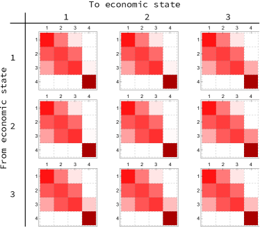
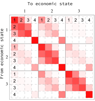
Refer to caption
Refer to caption
Figure 3: $M^{(a,b)}$ matrices (left) and $P$ matrix (right) of TTC rating. Economic states are labelled 1 (good), 2 (neutral) and 3 (bad). Darker shades indicate values closer to one, whereas white indicates a value of zero or close to zero.

Figure 1 in Section 2.2 shows the PIT $M^{(a,b)}$ matrices and $P$ matrix. Figure 3 shows the corresponding matrices of the TTC rating. The $M^{(a,b)}$ matrices reveal that, as expected, rating transitions in the PIT rating depend more strongly on the economic state transition, while transitions to non-default ratings of the TTC system vary little across economic state transitions. The PDs of TTC rating classes (last column in each matrix) show variation across the economic states. It is easily verified that the $P$ matrices are monotone with respect to the upper orthant order. They are even stochastically monotone, so powers are monotone with respect to the upper orthant order as well.

Refer to caption
Figure 4: Default curves generated by PIT (left) and TTC (right) ratings. Left, from top to bottom: initial PIT ratings are ordered from best to worst non-default rating; each curve denotes the economic state in which the curve starts (blue: good, red: neutral, green: bad). Right: Corresponding TTC ratings, where initial distributions $\lambda^{\text{TTC}}_{(a,r)},r\in\mathcal{\hat{R}},a\in\mathcal{A}$, are calibrated to respective initial PIT rating, see Equation (47).

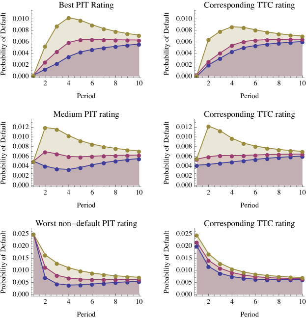
In the following, we compare various default curves generated by PIT and TTC ratings. The left-hand side of Figure 4 shows default curves for all combinations of initial PIT non-default ratings and economic states. The right-hand side shows the corresponding calibrated TTC ratings. Regardless of the economic state, the PIT one-period PD depends only on the initial PIT rating. This is not the case for TTC ratings, although default probabilities are close, given that each TTC default curve represents firms in one PIT rating. The default curves converge at the long end across ratings and economic states. Because TTC rating classes are more stable, due to the constant $Q$ matrix, convergence tends to occur faster.

Refer to caption
Figure 5: Default curves generated by TTC ratings. Colour-coded curves denote the initial economic state (blue: good, red: neutral, green: bad). The grey curve denotes the default probabilities of the asymptotic approximation (12), which corresponds to a TTC rating that has no economic-state information at all.

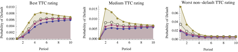
Figure 5 shows default curves for every combination of initial TTC rating and initial economic state. In each graph, the curves are again ordered according to the initial economic state (blue: good, red: neutral, green: bad). As the one-period PDs for the best and medium TTC ratings are practically zero, regardless of the economic state, a firm’s rating path will nearly certainly pass through the worst TTC rating before it defaults.

Also shown in Figure 5 (in grey) are default curves derived from the asymptotic approximation (12) of the TTC rating. As before, (conditional) rating migrations are insensitive to the economic state, but in addition, this is now also the case for PDs. These PDs meet regulatory capital requirements by being based on the observed historical average one-year default rate, Basel Committee on Banking Supervision (2016). It can be seen that these PDs over- or underestimate real PDs depending on the economic state.

Refer to caption
Figure 6: Default curves generated by PIT and TTC ratings where only the initial economic state is known. The initial distributions of the PIT and TTC ratings are determined from the stationary distribution of $P$. Colour-coded curves denote the initial economic state (blue: good, red: neutral, green: bad). The grey curve denotes the default probabilities of the asymptotic approximation (12), which corresponds to a TTC rating that has no economic-state information at all.

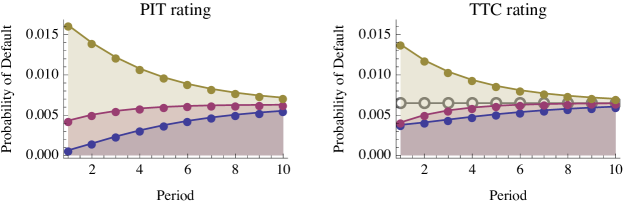
Finally, Figure 6 shows default curves of PIT and TTC ratings, where only the initial economic state is known. The initial distributions are chosen as the stationary distributions, which are determined from the $P$ matrices with default states removed, and then conditioned on each economic state. The curves can be interpreted as representing – conditional on the economic state – the default probabilities of a randomly picked firm. As such, ideally, the curves would be equal, as the default probabilities of a randomly picked firm should not depend on a particular rating philosophy. However, as can be seen, with the TTC rating being “more stable”, it is harder to differentiate the neutral and bad economic states than in the case of the PIT ratings where the initial default probabilities are given.

The grey curve in Figure 6 shows the default curve of the TTC rating’s asymptotic approximation (12). Given that there is no initial information about the firm and the economic state, these PDs remain constant through time.

8 Conclusion

To conclude, we point out how the rating framework introduced in this paper complies with requirements of ratings and PDs in both accounting and regulatory capital standards.

The International Financial Reporting Standard (IFRS) 9 as well as the accounting standard Current Expected Credit Losses (CECL) require financial institutions to calculate expected credit losses that reflect current economic conditions and forecasts of future economic conditions121212International Financial Reporting Standard (IFRS) 9, Paragraph 5.5.17. Hence, default probabilities that are used for calculating expected credit losses for accounting purposes have to be realistic estimates of the actual probability of default taking the current economic state as well as the future (stochastic) development of economic conditions into account. As the accounting standards do not contain any requirements on rating systems, even default probabilities of a rating process $(R_{t})_{t\in\mathbb{N}_{0}}$ that is predominantly TTC satisfies the accounting requirements as long as the PD curve ${{\mathbb{P}}(R_{t}=\overline{r})}_{t\in\mathbb{N}_{0}}$ specified by $(R_{t})_{t\in\mathbb{N}_{0}}$ provides a realistic estimate of the actual probabilities of default. This requirement typically implies that default probabilities ${\mathbb{P}}(R_{t+1}=\overline{r}|R_{t}=r)$ show a strong dependence on economic states to make up for the low sensitivity of non-default ratings to economic conditions if $(R_{t})_{t\in\mathbb{N}_{0}}$ is predominantly TTC.

The PD curve ${{\mathbb{P}}(R_{t}=\overline{r})}_{t\in\mathbb{N}_{0}}$ can be derived from the time-inhomogeneous transition matrices ${\widetilde{P}}_{t}$ via Equation (10). In our setup, the transition matrices ${\widetilde{P}}_{t}$ depend on the probabilities of the different economic paths $(a_{0},a_{1},\ldots,a_{t})\in{\mathcal{A}}^{t+1}$ specified by the Markov process $(A_{t})_{t\in\mathbb{N}_{0}}$. In practice, the specification of economic scenarios $(a_{0},a_{1},\ldots,a_{T})$ is based on actual macro-economic forecasts, which provide the economic information required for the transition matrices ${\widetilde{P}}_{1},\ldots,{\widetilde{P}}_{T}$ up to a forecast horizon $T$. For extending the default curve beyond $T$, the asymptotic transition matrix ${\widetilde{P}}_{\infty}$ is typically used, which formalizes the long-term average migrations of the rating process, see Equation (12).

In contrast to accounting requirements, financial regulators wish to avoid procyclical capitalisation of financial institutions, as this would incentivise firms to reduce their capital when the economy thrives, which in turn would require firms to increase their capital in economic downturns, when this is particularly difficult to achieve. As this procyclical capitalisation poses a threat to financial stability, financial regulators prefer banks to assess regulatory capital requirements for credit risk using through-the-cycle (TTC) ratings,131313Capital requirements regulation and directive – CRR/CRD IV, Article 502 which are designed to be stable through the business cycle. In addition, default probabilities in regulatory capital requirement calculations should be based on the observed historical average one-year default rate, see Basel Committee on Banking Supervision (2016). In order to satisfy these requirements in our setup, consider a rating migration process $(R_{t})_{t\in\mathbb{N}_{0}}$ that is predominantly TTC. The asymptotic PDs of $(R_{t})_{t\in\mathbb{N}_{0}}$ correspond to the historical average one-year default rate of this rating migration process. Hence, the asymptotic approximation $(S_{t})_{t\in\mathbb{N}_{0}}$ based on the transition matrix ${\widetilde{P}}_{\infty}$ (see Definition 4.2) is a rating migration process that is consistent with the regulatory requirements listed above. However, as the example in Section 7.3 demonstrates, $(S_{t})_{t\in\mathbb{N}_{0}}$ does not provide realistic PD estimates. In particular, these PDs – shown in Figures 5 and 6 – tend to underestimate the actual default risk in a negative economic environment. Alternatively, the asymptotic default probabilities specified by ${\widetilde{P}}_{\infty}$ could be replaced by default probabilities taken from a conditional transition matrix $M^{(a,b)}$, where the choice of the economic states $a,b\in{\mathcal{A}}$ reflects the underlying economic assumptions. For example, if the transition from $a$ to $b$ represents a negative economic scenario the default probabilities in $M^{(a,b)}$ could be interpreted as stressed PDs. If default probabilities are specified in this way the underestimation of the actual default risk could be avoided, even in a negative economic environment, but at the expense of overly conservative PD estimates during benign economic times.

References

  • Aguais et al. (2008) Aguais, S. D., L. R. Forest, M. King, M. C. Lennon, and B. Lordkipanidze. Designing and Implementing a Basel II Compliant PIT-TTC Ratings Framework. In The Basel Handbook. Risk Books, 2nd edition, 2008.
  • Altman and Rijken (2004) Altman, E. I. and H. A. Rijken. How rating agencies achieve rating stability. Journal of Banking & Finance, 28(11):2679–2714, 2004.
  • Altman (1998) Altman, E. I. The importance and subtlety of credit rating migration. Journal of Banking & Finance, 22(10-11):1231–1247, 1998.
  • Bangia et al. (2002) Bangia, A., F. X. Diebold, A. Kronimus, C. Schagen, and T. Schuermann. Ratings migration and the business cycle, with application to credit portfolio stress testing. Journal of Banking & Finance, 26:445–474, 2002.
  • Basel Committee on Banking Supervision (2016) Basel Committee on Banking Supervision. Reducing variation in credit risk-weighted assets - constraints on the use of internal model approaches. Consultative Document, 2016.
  • Behn et al. (2016) Behn, M., R. Haselmann, and P. Wachtel. Procyclical capital regulation and lending. The Journal of Finance, 71(2):919–956, 2016.
  • Bluhm and Overbeck (2007) Bluhm, C. and L. Overbeck. Calibration of PD term structures: to be Markov or not to be. Risk, 20(11):98–103, 2007.
  • Bluhm et al. (2003) Bluhm, C., L. Overbeck, and C. Wagner. An Introduction to Credit Risk Modeling. Chapman & Hall/CRC, London, 2003.
  • Borio et al. (2001) Borio, C., C. Furfine, and P. Lowe. Procyclicality of the financial system and financial stability: issues and policy options. BIS papers, No. 1, 2001.
  • Brémaud (1999) Brémaud, P. Markov chains: Gibbs fields, Monte Carlo simulation, and Queues, volume 31. Springer, 1999.
  • Carlehed and Petrov (2012) Carlehed, M. and A. Petrov. A methodology for point-in-time-through-the-cycle probability of default decomposition in risk classification systems. The Journal of Risk Model Validation, 6(3):3, 2012.
  • Crouhy et al. (2001) Crouhy, M., D. Galai, and R. Mark. Prototype risk rating system. Journal of Banking & Finance, 25(1):47–95, 2001.
  • Duffie and Singleton (2003) Duffie, D. and K. J. Singleton. Credit Risk: Pricing, Measurement, and Management. Princeton University Press, 2003.
  • Fei et al. (2012) Fei, F., A.-M. Fuertes, and E. Kalotychou. Credit rating migration risk and business cycles. Journal of Business Finance & Accounting, 39(1-2):229–263, 2012.
  • Föllmer and Schied (2002) Föllmer, H. and A. Schied. Stochastic Finance. An Introduction in Discrete Time. de Gruyter, 2002.
  • Frobenius (1912) Frobenius, G. Über Matrizen aus nicht negativen Elementen. Sitzungsberichte der Königlich Preussischen Akademie der Wissenschaften, pages 456–477, 1912.
  • Frydman and Schuermann (2008) Frydman, H. and T. Schuermann. Credit rating dynamics and markov mixture models. Journal of Banking & Finance, 32(6):1062–1075, 2008.
  • Gera (2020) Gera, I. Credit rating migration processes based on economic state-dependent transition matrices. Master’s thesis, Goethe-University Frankfurt, 2020.
  • Gordy and Howells (2004) Gordy, M. B. and B. Howells. Procyclicality in Basel II: Can we treat the disease without killing the patient? Working Paper, Board of Governors of the Federal Reserve System, April 2004.
  • Güttler and Raupach (2010) Güttler, A. and P. Raupach. The impact of downward rating momentum. Journal of Financial Services Research, 37(1):1, 2010.
  • Heitfield (2005) Heitfield, E. A. Dynamics of rating systems. In Studies on the Validation of Internal Rating Systems. BIS Working Papers, No. 14, 2005.
  • Jarrow et al. (1997) Jarrow, R. A., D. Lando, and S. M. Turnbull. A Markov model for the term structure of credit risk spreads. Review of Financial Studies, 10(2):481–523, 1997.
  • Lando and Skødeberg (2002) Lando, D. and T. M. Skødeberg. Analyzing rating transitions and rating drift with continuous observations. Journal of Banking & Finance, 26(2-3):423–444, 2002.
  • Lando (2004) Lando, D. Credit Risk Modeling. Princeton University Press, 2004.
  • Lemmon et al. (2008) Lemmon, M. L., M. R. Roberts, and J. F. Zender. Back to the beginning: persistence and the cross-section of corporate capital structure. Journal of Finance, 63(4):1575–1608, 2008.
  • Malik and Thomas (2012) Malik, M. and L. C. Thomas. Transition matrix models of consumer credit ratings. International Journal of Forecasting, 28(1):261–272, 2012.
  • Merton (1974) Merton, R. C. On the pricing of corporate debt: The risk structure of interest rates. Journal of Finance, 29(2):449–470, May 1974.
  • Miu and Ozdemir (2017) Miu, P. and B. Ozdemir. Adapting the Basel II advanced internal-ratings-based models for International Financial Reporting Standard 9. Journal of Credit Risk, 13(2):53–83, 2017.
  • Morone and Cornaglia (2009) Morone, M. and A. Cornaglia. Rating philosophy and dynamic properties of internal rating systems: a general framework and an application to backtesting. Journal of Risk Model Validation, 3(4):61–88, 2009.
  • Müller and Stoyan (2002) Müller, A. and D. Stoyan. Comparison methods for stochastic models and risks, volume 389. Wiley, 2002.
  • Müller (2013) Müller, A. Stochastic Orders in Reliability and Risk, chapter Duality Theory and Transfers for Stochastic Order Relations, pages 41–57. Springer New York, 2013.
  • Nickell et al. (2000) Nickell, P., W. Perraudin, and S. Varotto. Stability of rating transitions. Journal of Banking & Finance, 24:203–227, 2000.
  • Norris (1998) Norris, J. R. Markov Chains. Cambridge University Press, 1998.
  • Perron (1907) Perron, O. Zur Theorie der Matrices. Mathematische Annalen, 64(2):248–263, 1907.
  • Rolski et al. (2009) Rolski, T., H. Schmidli, V. Schmidt, and J. L. Teugels. Stochastic processes for insurance and finance. John Wiley & Sons, 2 edition, 2009.
  • Rosenblatt (1971) Rosenblatt, M. Markov processes, Structure and Asymptotic Behavior. Springer, 1971.
  • Rubtsov and Petrov (2016) Rubtsov, M. and A. Petrov. A point-in-time-through-the-cycle approach to rating assignment and probability of default calibration. Journal of Risk Model Validation, 10(2):83–112, 2016.
  • Rubtsov (2021) Rubtsov, M. Calibration of rating grades to point-in-time and through-the-cycle levels of probability of default. Journal of Risk Model Validation, 2021.
  • Seneta (1973) Seneta, E. Non-negative matrices. George Allen & Unwin Ltd, 1973.
  • Shaked and Shanthikumar (2007) Shaked, M. and J. G. Shanthikumar. Stochastic orders. Springer Science & Business Media, 2007.
  • Vallés (2006) Vallés, V. Stability of a ”through-the-cycle” rating system during a financial crisis. Financial Stability Institute, Bank of International Settlements (BIS), 2006.
  • Wilson (1998) Wilson, T. C. Portfolio credit risk. Federal Reserve Bank of New York Economic Policy Review, 1998.