Learning Quadruped Locomotion Using
Differentiable Simulation

Abstract

While most recent advancements in legged robot control have been driven by model-free reinforcement learning, we explore the potential of differentiable simulation. Differentiable simulation promises faster convergence and more stable training by computing low-variant first-order gradients using the robot model, but so far, its use for legged robot control has remained limited to simulation. The main challenge with differentiable simulation lies in the complex optimization landscape of robotic tasks due to discontinuities in contact-rich environments, e.g., quadruped locomotion. This work proposes a new, differentiable simulation framework to overcome these challenges. The key idea involves decoupling the complex whole-body simulation, which may exhibit discontinuities due to contact, into two separate continuous domains. Subsequently, we align the robot state resulting from the simplified model with a more precise, non-differentiable simulator to maintain sufficient simulation accuracy. Our framework enables learning quadruped walking in minutes using a single simulated robot without any parallelization. When augmented with GPU parallelization, our approach allows the quadruped robot to master diverse locomotion skills, including trot, pace, bound, and gallop, on challenging terrains in minutes. Additionally, our policy achieves robust locomotion performance in the real world zero-shot. To the best of our knowledge, this work represents the first demonstration of using differentiable simulation for controlling a real quadruped robot. This work provides several important insights into using differentiable simulations for legged locomotion in the real world.

I Introduction

Many grazing animals, such as giraffes, lambs, and calves, can learn to stand and walk within minutes to hours after birth. On the other hand, most machine learning algorithms, particularly traditional model-free reinforcement learning (RL), need massive parallelization to achieve a stable walking policy. How can legged robots master walking in minutes with a few trials and errors?

Recent progress in legged robot control has largely been driven by GPU-accelerated massive simulation and reinforcement learning [15, 20, 24, 30, 22, 9, 39, 19]. Central to these advancements is the policy gradient algorithm [35, 34, 6]. The policy gradient can generally be expressed as the following

$$\nabla_{\theta}J(\theta)\approx\mathbb{E}[\nabla_{\theta}\log\pi_{\theta}(u_{t}|x_{t})R_{t}(\bm{\tau})],$$

where it stands as a zeroth-order approximation of the true gradient based on sampled trajectories $\bm{\tau}$. Here, $R_{t}(\bm{\tau})$ represents the sum of future rewards. Despite impressive real-world performance, this approach to gradient estimation is known for its high variance. Consequently, several additional strategies are required for stable training, such as using a clipped surrogate objective [31], increasing the number of samples, designing task-specific learning curriculums, employing distributed initialization techniques, and engineering suitable reward functions.

As a result, RL struggles with complex tasks where data generalization is slow, like vision-based navigation. Despite the need for more effective learning algorithms, progress has been limited. Instead, research leans towards imitation learning, utilizing existing datasets or expert demonstrations for more consistent learning outcomes. Notably, the learning-by-cheating approach [4] is a popular imitation learning framework: first, you train an RL teacher with privileged information and then, you derive a student policy based on visual inputs. However, the success of this approach heavily depends on the quality of expert demos and lacks generalizability and adaptability to new tasks.

In robotics, leveraging well-established knowledge about robot dynamics can enable the construction of first-order gradient estimations, which typically exhibit significantly lower variance than their zeroth-order counterparts and hold great potential for more stable training and faster convergence. Recently, policy training using first-order gradient has been notably advanced through differentiable simulation [8, 14, 36, 29, 37]; these works have shown promising results in reducing both the number of simulation samples and total training time compared to zeroth-order methods.

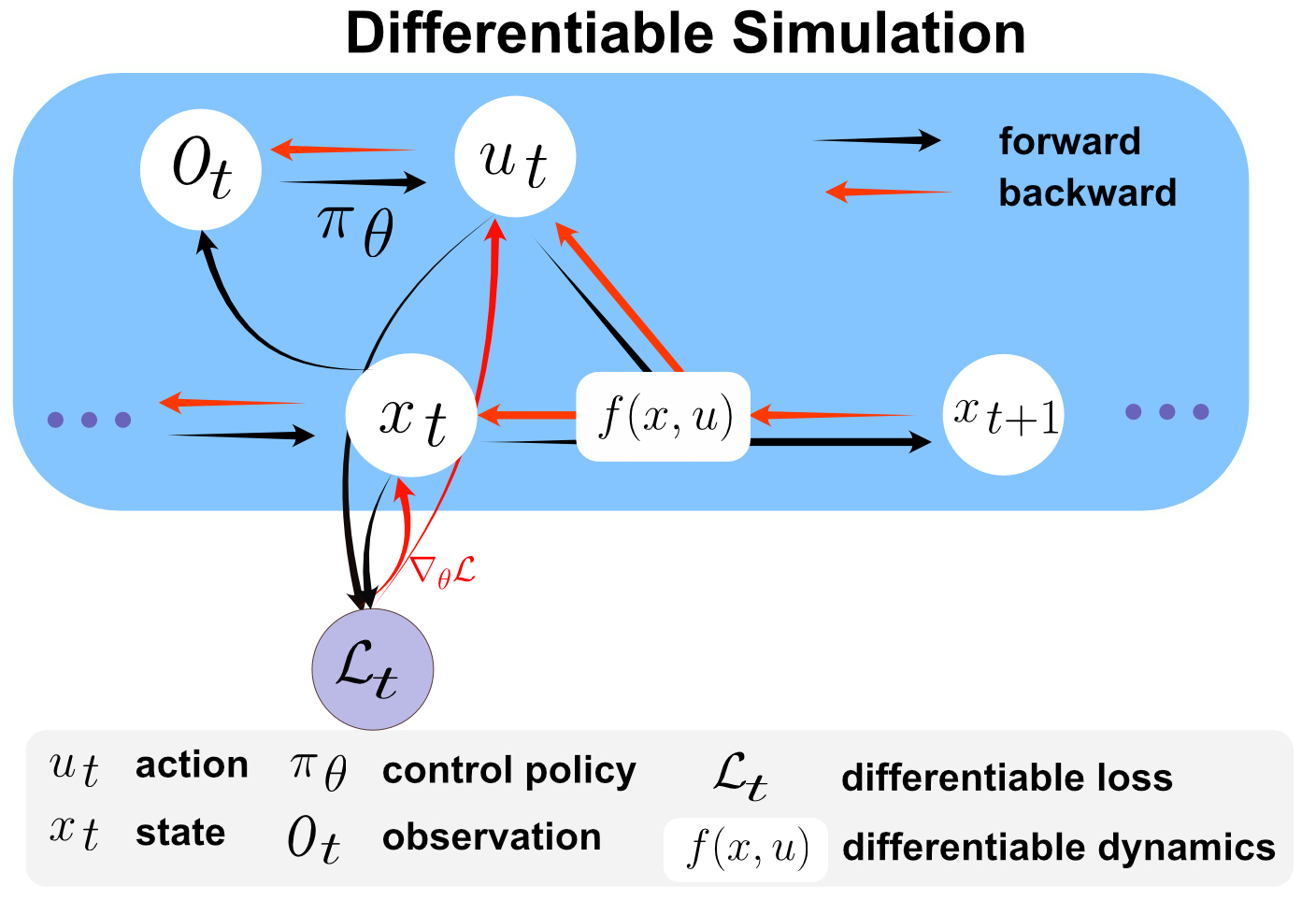
Figure 1: Graphical model for policy learning using differentiable simulation, in which both the loss function and the dynamics are differentiable.

However, the optimization landscape in robotic tasks is inherently complex, characterized by nonlinearities, non-smooth and discontinuous dynamics, non-convexities, and long temporal horizons. Additionally, deploying real-world robots introduces additional challenges, such as the sim-to-real gap, noisy state estimation, and system delay. Consequently, policy training through differentiable simulation can suffer from issues like local minimum and gradient vanishing/explosion. While differentiable simulation offers a promising avenue, its effectiveness in significantly accelerating policy learning in contact-rich environments and its applicability to real-world scenarios like dynamic quadruped control remains an open challenge in robotics.

This work set out to explore the potential of differentiable simulation in accelerating policy training within contact-rich scenarios like dynamic legged locomotion. Our goal is to establish an effective policy training framework that leverages the robot model for precise gradient computation while mitigating the difficulties posed by complex, discontinuous optimization landscapes. Moreover, we intend to evaluate the strengths and weaknesses of this approach in comparison to zeroth-order methods, particularly model-free policy gradients. We aim to provide useful insights for developing more efficient and robust methods that benefit from both worlds.

Contribution: We show that differentiable simulation offers considerable advantages over model-free reinforcement learning for policy training in legged locomotion. Notably, we demonstrate that a single robot, without the need for parallelization, can quickly learn to walk within minutes using our approach. Leveraging the advantage of GPUs for parallelized simulation, our robot learns diverse walking skills over challenging terrain in minutes. Specifically, we train a quadruped robot to walk with different gait patterns, including trot, pace, bound, and gallop, and with varying gait frequencies. While model-free RL can also achieve similar performance given sufficient parallelization, our approach requires much less data and yields better performance.

More importantly, we show that the policy trained via differentiable simulation can be transferred to the real world directly without fine-tuning. To the best of our knowledge, this work represents the first demonstration of using differentiable simulation for controlling a real quadruped robot. This highlights the effectiveness of differentiable simulation for real-world applications in dynamic legged locomotion scenarios.

The key to our approach is a novel policy training framework that combines the smooth gradients obtained from a simplified dynamics model for efficient backpropagation with the high fidelity of a more complex, non-differentiable simulator for accurate forward simulation. 1) Decoupling Simulation Spaces: Rather than handling the whole body dynamics as a unified differentiable simulator, which may encounter non-smoothness due to contact interactions. We proposed to separate the simulation into two distinct spaces: the floating base space and the joint space. For the robot body, we employ an approximation using single rigid-body dynamics, which offers a continuous and effective representation of the floating base (the robot body). 2) PD Control as A Differentiable Layer: The simulation within the joint space benefits from the inherent differentiability and smoothness of a Proportional-Derivative (PD) controller. This allows us to treat the PD control as an explicit, differentiable layer within our simulation framework. 3) Alignment with Non-Differentiable Simulators: To address potential inaccuracies arising from our simplified rigid-body dynamics model, we incorporate a more precise, non-differentiable simulator. This non-differentiable simulator can simulate complex contact dynamics and is used to align our simplified model, thereby ensuring that our training pipeline remains grounded in realistic dynamics.

II Related Work

II-A Model Predictive Control

Model predictive control (MPC) has a long history in legged locomotion [18, 16]. MPC relies on fast online optimization and an accurate dynamics model to control the robot. To trade-off between model accuracy and computation speed, many methods use a reduced optimization model, such as single rigid-body dynamics [7, 11, 2]. Research has also studied control using more complex formulations, including centroidal [10] and whole-body dynamics [26]. Despite their success, MPC lacks the flexibility in its optimization objective design and robustness when facing disturbances or unexpected scenarios. Empirical evidence suggests that MPC tends to underperform when compared to data-driven approaches such as deep reinforcement learning.

II-B Reinforcement Learning

Deep reinforcement learning has emerged as a dominant approach for developing control policies in legged locomotion [15, 20, 24, 19]. Recently, an important advancement in this area has been the introduction of IsaacGym [21], which is a GPU-accelerated simulator. IsaacGym can dramatically reduce the time required for dynamics simulation and policy training, enabling robots to learn to walk on flat ground in minutes [30]. This advancement has significantly accelerated the pace of research in legged locomotion, opening new avenues to address increasingly complex challenges [38, 1, 9, 22, 39].

Nevertheless, it is important to highlight that the progress in applying reinforcement learning to legged locomotion is primarily driven by the enhanced computational capabilities provided by modern GPUs rather than substantial breakthroughs in the underlying algorithms. Consequently, in scenarios where data collection cannot be accelerated through computational means, researchers may resort to alternative strategies such as “learning-by-cheating” to circumvent these limitations. This highlights a gap in the current approach to deep RL in legged locomotion, suggesting a need for innovative algorithmic developments that do not solely rely on computational advancements.

II-C Differentiable Simulation

Differentiable simulation has recently gained momentum, thanks to the development of differentiable physics simulators [8, 5, 12] and flexible automatic differentiation tools like Jax, DiffTaichi, Pytorch [3, 13, 27]. In principle, policy training through differentiable simulation allows better convergence by replacing the zeroth-order gradient estimation of a stochastic objective with a more accurate estimate based on first-order gradients [33]. However, challenges such as the noisy optimization landscape and issues of exploding or vanishing gradients in long-horizon tasks render first-order gradient methods less effective.

Several approaches have been developed to tackle these challenges. For instance, SHAC [36] addresses the gradient issue by truncating trajectories into several smaller segments, which helps manage exploding or vanishing gradients. On the other hand, PODS [25] takes advantage of second-order gradients. This approach facilitates monotonic policy improvement and promises faster convergence than first-order methods. However, PODS’ effectiveness relies on very accurate computation of second-order derivatives from the differentiable simulator, making it sensitive to the precision of these derivatives. Another notable example is DiffMimic [29], which focuses on mimicking motion trajectories for physically simulated characters.

Research in differentiable simulation has mainly been focused on speeding up policy optimization using first-order gradients, alleviating local minima problems, addressing gradient vanishing/explosion issues, or developing control policies for simulated characters. They show that differentiable simulation is a promising direction for improving sample efficiency. However, the capability of differentiable simulation to substantially speed up policy learning in contact-rich scenarios with physical interactions, as well as their practical applicability to real-world situations, such as quadruped locomotion, continues to be a significant challenge in robotics.

Our research distinguishes itself from earlier studies by presenting a novel perspective that leads to an effective solution tailored for real-world robotic applications.

III Methodology

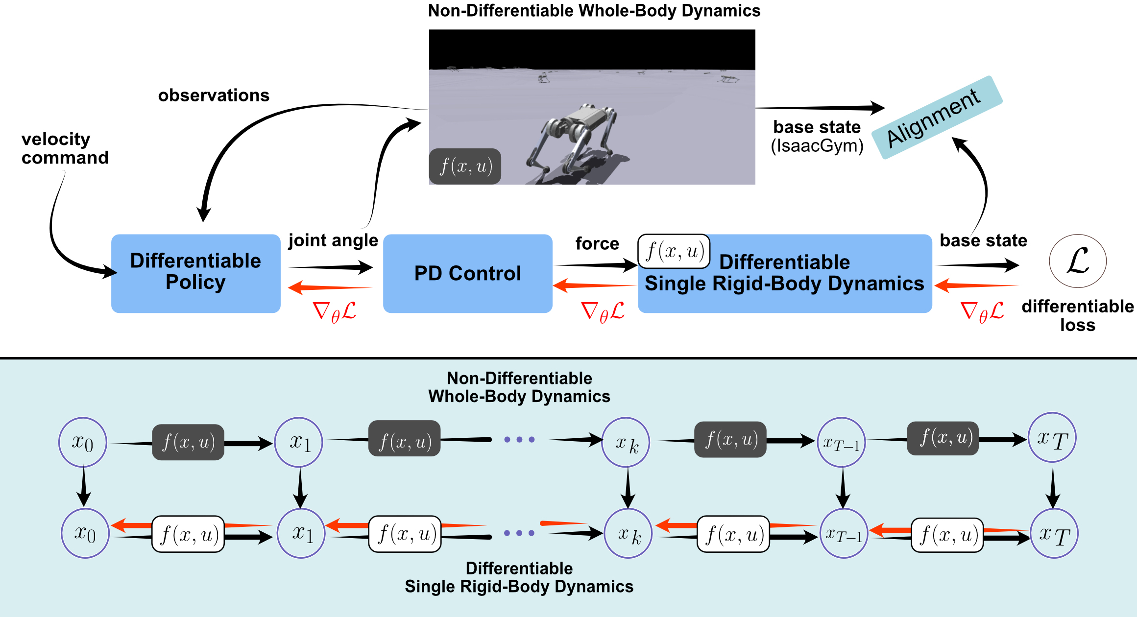
Figure 2: System overview of legged robot control using differentiable simulation. Our approach leverages the differentiability and smoothness of a single rigid-body dynamics for dynamics simulation. Additionally, we treat PD control as a differential layer in our computation graph. Finally, we use the state from a more accurate, non-differentiable simulator (IsaacGym) to align the simulated state in the simple rigid-body simulation.

III-A Overview

Fig. 2 shows our training setup that employs differentiable simulation. The fundamental idea is that the main body of a legged robot can be modeled using differentiable and smooth single rigid-body dynamics, while the simulation of the robot’s four legs can be approached separately from its main body. We use a Proportional-Derivative (PD) controller to connect the legs dynamics with the main body. In the forward pass, this PD controller converts joint angles into torques, which then produce the contact forces needed for the robot’s rigid-body simulation. During backpropagation, the PD controller functions as a differentiable component, enabling gradients to be propagated back through the system. Finally, we use non-differentiable whole-body dynamics simulation to align the state produced by our simplified rigid-body dynamics.

III-B Problem Formulation

We formulate legged robot control as an optimization problem. The robot is modeled as a discrete-time dynamical system, characterized by continuous state and control input spaces, denoted as $\mathcal{X}$ and $\mathcal{U}$, respectively. At each time step $k$, the system state is $x_{k}\in\mathcal{X}$, and the corresponding control input is $u_{k}\in\mathcal{U}$. An observation $o_{k}\in\mathcal{O}$ is generated at each time step based on the current state $x_{k}$ through a sensor model $h:\mathcal{X}\rightarrow\mathcal{O}$, such that $o_{k}=h(x_{k})$. The system’s dynamics are governed by the function $f:\mathcal{X}\times\mathcal{U}\rightarrow\mathcal{X}$, which describes the time-discretized evolution of the system as $x_{k+1}=x_{k}+\Delta t\cdot f(x_{k},u_{k})$. The discrete-time instants are $t_{k}=\Delta t\cdot k$, where $k$ ranges from 0 to $N$, thereby establishing a finite time horizon for the control problem. At each time step $k$, the robot receives a cost signal $l_{k}=l(x_{k},u_{k})$, which is a function of the current state $x_{k}$ and the control input $u_{k}$.

The control policy is represented as a deterministic, differentiable function such as a neural network $u_{k}=\pi_{\theta}(o_{k})$. The neural network takes the observation $o_{k}$ as input and outputs the control input $u_{k}$. The optimization objective is to find the optimal policy parameters $\theta^{\ast}$ by minimizing the total loss via gradient descent:

$$\min_{\theta}\mathcal{L}_{\theta} =\sum_{k=0}^{N-1}l(x_{k},u_{k})=\sum_{k=0}^{N-1}l(x_{k},\pi_{\theta}(o_{k}))$$ (1)

$$\theta \leftarrow\theta-\alpha\nabla_{\theta}\mathcal{L}_{\theta}$$ (2)

where $\alpha$ is the learning rate and $l(x_{k},u_{k})$ is the differentiable loss at simulation time step $k$.

III-C Forward Simulation

Legged robots are characterized by complex dynamics resulting from their multi-body configuration and the contact between their body and the environment. The contacts introduce discontinuities in the dynamics, making first-order gradient-based optimization algorithms difficult. An important aspect of our approach involves separating the simulation of the robot’s body from that of its joints. This design choice allows a simple implementation of the differentiable simulator.

First, we represent the robot’s main body using single rigid-body dynamics. Single rigid-body dynamics have been shown to be useful for dynamic locomotion using online gradient-based optimization [7, 11]. The single rigid-body model offers a continuous representation of the robot base dynamics, avoiding the complex optimization landscape introduced by contacts. We develop our differentiable simulation using the single rigid-body dynamics, which is expressed as follows,

$$\dot{\mathbf{p}}_{WB} =\mathbf{v}_{WB} \dot{\mathbf{v}}_{WB} =\frac{1}{m}\sum_{i}\mathbf{f}_{i}+\mathbf{g}$$

$$\dot{\mathbf{q}}_{WB} =\frac{1}{2}\Lambda(\bm{\omega}_{B})\cdot\mathbf{q}_{WB} \dot{\bm{\omega}}_{B} =\mathbf{I}^{-1}\left(\bm{\eta}-\bm{\omega}_{B}\times(\mathbf{I}\bm{\omega}_{B})\right)$$

In this approximation, the state of our system is

$$\mathbf{x}=[\mathbf{p},\mathbf{q},\mathbf{v},\bm{\omega}],$$

where $\mathbf{p}_{\text{WB}}\in\mathbb{R}^{3}$ is the position and $\mathbf{v}_{\text{WB}}\in\mathbb{R}^{3}$ is the linear velocity of the center of mass in the world frame ${W}$, We use a unit quaternion $\mathbf{q}_{\text{WB}}$ to represent the orientation of the body in the world frame and use $\bm{\omega}_{\text{B}}$ to denote the body rates in the body frame ${B}$. Here, $\mathbf{\Lambda}(\bm{\omega}_{B})$ is a skew-symmetric matrix. The control inputs are the ground reaction force $\mathbf{f}_{i}$ from the legs.

To simulate the rigid-body dynamics, it is important to know the ground reaction force. One option for the control policy design is to output the ground reaction force directly, similar to the MPC design [7, 11]. Another option is to control the robot in the joint space, e.g., output desired joint position, which allows more control authority for the policy and adaptive behavior. In this case, it is required to convert the neural network output (joint position) into the control input of the single rigid-body model, which is the ground reaction force. This conversion is achieved using a PD controller for forward propagation,

$$\bm{\tau}=\mathbf{k_{p}(q^{\text{ref}}-q)}+\mathbf{k_{d}(\dot{q}^{\text{ref}}-\dot{q})}$$ (3)

which calculates the required motor torque $\bm{\tau}$. Here, $\mathbf{k_{p}}$ and $\mathbf{k_{d}}$ are fixed gains, $\mathbf{q^{\text{ref}}}$ and $\mathbf{q}$ are the reference joint position and the current joint position separately, and $\mathbf{\dot{q}^{\text{ref}}}$ and $\mathbf{\dot{q}}$ are the reference joint velocity and the current joint velocity respectively.

Subsequently, the motor torques are then converted to ground reaction forces $\mathbf{f}$ using the foot Jacobian $\mathbf{J}$:

$$\mathbf{f}=(\mathbf{J}^{T})^{-1}\bm{\tau}.$$

The continuous nature of PD control enables the backpropagation of policy gradients. Consequently, our simulation framework treats the PD controller as an explicit, differentiable layer.

III-D Backpropagation Through Time

In differentiable simulation for policy learning, the backward pass is crucial for computing the analytic gradient of the objective function with respect to the policy parameters. Following [23], the policy gradient can be expressed as follows

$$\frac{\partial\mathcal{L}_{\theta}}{\partial\theta} =\frac{1}{N}\sum_{k=0}^{N-1}\left(\sum_{i=1}^{k}\frac{\partial l_{k}}{\partial x_{k}}\prod_{j=i}^{k}\left(\frac{\partial x_{j}}{\partial x_{j-1}}\right)\frac{\partial x_{i}}{\partial\theta}+\frac{\partial l_{k}}{\partial u_{k}}\frac{\partial u_{k}}{\partial\theta}\right),$$ (4)

where the matrix of partial derivatives $\partial x_{j}/\partial x_{j-1}$ is the Jacobian of the dynamical system $f$. Therefore, we can compute the policy gradient directly by backpropagating through the differentiable physics model and a loss function $l_{k}$ that is differentiable with respect to the system state and control inputs. A graphical model for gradient backpropagation in policy learning using differentiable simulation is given in Fig. 1. Due to the usage of multiplication $\prod$, there are two potential issues in using Eq. (4) for policy gradient: 1) gradient vanishing or exploding, 2) long computation time. We tackle these two problems via short-horizon policy training.

III-E Short-Horizon Policy Training

Although smoothed physical models (e.g., single rigid-body dynamics) improve the local optimization landscape, the complexity of the optimization problem escalates significantly in long-horizon problems involving extensive concatenation of simulation steps. The situation further deteriorates when the actions within each step are interconnected through a nonlinear and nonconvex neural network control policy. The complexity of the resulting reward landscape leads simple gradient-based methods to become trapped in local optima quickly. Instead of directly solving a long-horizon policy training problem, following [36, 30], where long-horizon simulation tasks are truncated into short-horizon simulation, we utilize short-horizon policy learning to achieve stable gradient backpropagation over a short horizon.

III-F Alignment with A Non-Differentiable Simulator

Due to the simplification of our single rigid-body dynamics, the robot state can diverge from its actual one, eventually leading to unrealistic states due to compounding errors. We proposed to align the body state in our differentiable simulation using information from other simulators that use accurate whole-body dynamics. Specifically, we align the robot state in our differentiable simulation with the state information from IsaacGym [21].

We use the following equation to align the robot state.

$$\mathbf{x}^{\text{diff}}_{t+1}=\mathbf{x}^{\text{non-diff}}_{t+1}+\alpha*(\mathbf{x}^{\text{diff}}_{t+1}-\mathbf{x}^{\text{diff, detach}}_{t+1})$$ (5)

Here, $\mathbf{x}^{\text{diff, detach}}_{t+1}$ and $\mathbf{x}^{\text{diff}}_{t+1}$ represent the same robot state of our differentiable simulator at time step $t+1$; hence, they share the same value. The word detach indicates that $\mathbf{x}^{\text{diff, detach}}_{t+1}$ is detached from the computational graph for automatic differentiation. Therefore, we can reset the robot state using the value from the non-differentiable simulation during forward simulation: $\mathbf{x}^{\text{diff}}_{t+1}=\mathbf{x}^{\text{non-diff}}_{t+1}+\alpha*\bm{0}$. During backpropagation, the gradient of the state at a given time $t$ is computed as follows

$$\partial\mathbf{x}^{\text{diff}}_{t+1}/\partial\mathbf{x}^{\text{diff}}_{t}=\bm{0}+\alpha*\partial\mathbf{x}^{\text{diff}}_{t+1}/\partial\mathbf{x}^{\text{diff}}_{t}.$$ (6)

Here, $0<\alpha\leq 1$ is used to decay the gradient.

The non-differentiable simulator can simulate complex contact dynamics and is used to align our simplified model, thereby ensuring that our differentiable training pipeline remains grounded in realistic dynamics. At the same time, our approach benefits from the simplified differentiable simulator, which offers smooth gradients for backpropagation. Fig. 2 shows the computational graph of the forward propagation and backpropagation using alignment.

III-G Differentiable Loss Function

A fundamental difference between policy training using differentiable simulation and reinforcement learning is that the loss function has to be differentiable when using differentiable simulation. On the one hand, RL allows the direct optimization of non-differentiable rewards, such as binary rewards $0/1$. On the other hand, differentiable simulation requires a smooth differentiable cost function to provide learning signals for the desired control inputs.

We formulate a loss function tailored for velocity tracking, where the main objective is to follow a specified velocity command, denoted as $\mathbf{v}^{\text{ref}}$. Additionally, we maintain the robot’s body height, represented by $p_{z}$. To enhance the robustness of this system, we incorporate several regularization terms: one to mitigate large angular velocity, thus controlling the body rate; another to limit the output action, preventing large control actions; and a term aimed at stabilizing the robot’s orientation using projected gravity vector.

$$l(\mathbf{x}_{t},\mathbf{u}_{t}) = b\|\mathbf{v}-\mathbf{v}^{\text{ref}}\|^{2}+a\|p_{z}-p_{z}^{\text{ref}}\|+c\|\bm{\omega}\|^{2}$$ (7)

$$+d\|\mathbf{u}\|^{2}+f\|\mathbf{g}_{\text{proj}}\|+g\|\mathbf{p}_{\text{foot}}-\mathbf{p}_{\text{foot}}^{\text{ref}}\|^{2}$$

Finally, we use a foot position loss function to provide a learning signal for the swing legs. This loss is critical for the swing leg since it contains information about the motor position. The swing trajectory is computed by fitting a quadratic polynomial over the lift-off, mid-air, and landing position of each foot, where the lift-off position is the foot location at the beginning of the swing phase, the landing position is calculated using the Raibert Heuristics [28].

IV Experimental Setup

Simulation Setup: We develop our own differentiable simulation using PyTorch and CUDA. Our differentiable simulator allows both forward propagation of the robot dynamics and backpropagation of the policy gradient. Additionally, we run IsaacGym alongside our differentiable simulation and use it to align the robot state resulting from our simplified robot dynamics. IsaacGym simulates the whole-body dynamics and complicated contacts between the robot and its environment. Both simulations are parallelized on GPU. We use a discretized simulation time step of $0.002\text{\,}\mathrm{s}$ and use a control frequency of $100\text{\,}\mathrm{Hz}$.

Observation and Action: The policy observation includes random commands ($\textbf{cmd}_{\text{rand}}$) for the reference velocity, sinusoidal and cosinusoidal representations of gait phases, the base velocity ($\mathbf{v}_{WB}$), the base orientation ($\mathbf{q}_{WB}$), the angular velocity ($\bm{\omega}_{B}$), motor position deviations from default ($\mathbf{q}-\mathbf{q}_{\text{default}}$), and a projected gravity vector ($\mathbf{g}_{\text{projected}}$). The policy action $\delta\mathbf{q}$ is the desired joint position offset from the default joint position.

Observation	Dimension	Action	Dimension
$\textbf{cmd}_{\text{rand}}$	3	$\delta\mathbf{q}$	12
$\bm{\sin}(\text{gait phase})$	4
$\bm{\cos}(\text{gait phase})$	4
$\mathbf{v}_{WB}$	3
$\mathbf{q}_{WB}$	4
$\bm{\omega}_{B}$	3
$\mathbf{q}-\mathbf{q}_{\text{default}}$	12
$\mathbf{g}_{\text{projected}}$	3

TABLE I: Policy observation and action.

Hardware: We use Mini Cheetah [17] for our real-world experiments. Mini Cheetah is a small and inexpensive, yet powerful and mechanically robust quadruped robot, intended to enable rapid development of control systems for legged robots. The robot uses custom back-driveable modular actuators, which enable high-bandwidth force control, high force density, and robustness to impacts [17]. The control policy runs at $100\text{\,}\mathrm{Hz}$ during deployment.

V Experimental Results

V-A Learning to Walk with One Robot

This section explores whether a robot can learn to walk in a single simulation environment without parallelization. We design a simple velocity tracking task where the robot is required to follow a constant velocity in the $x$-axis, e.g., $v_{x}=0.2~{}m/s$. At each training iteration, we simulate 24 times steps with one single robot. Hence, each training iteration contains only 24 data points. We trained the policy for a total 1000 iterations, which corresponded to 24,000 data points and 4 minutes of real-time experiences in total. The result is given by the learning curve in Fig. 3. Surprisingly, despite extremely limited data, our policy successfully learns to walk after minutes of training. As a comparison, model-free reinforcement learning failed to yield positive outcomes under the same condition.

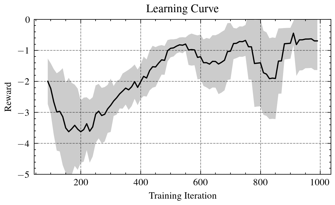
Figure 3: Learning to walk with one simulated robot. We run 10 experiments with different random seeds. The plot is smoothed using a moving average.

V-B Learning Diverse Walking Skills on Challenging Terrains

Though our approach enables tracking a constant velocity using one simulated robot on flat ground, it is generally helpful to parallelize the simulation for more complex tasks. To this end, we design a more difficult task: learning diverse locomotion skills over challenging terrains. Specifically, we design four different gait patterns, including trot, pace, bound, and gallop. Additionally, we vary the gait frequency from $1\text{\,}\mathrm{Hz}$ to $4\text{\,}\mathrm{Hz}$. The robot receives a high-level velocity command and is required to track randomly commanded velocity and yaw.

Fig. 5 shows the learning curves using different numbers of robots for policy training. We compare the learning performance of our method with a model-free RL algorithm (PPO) [31]. Given minimal samples, e.g., only four robots, RL has a plodding convergence speed and does not learn meaningful walking skills, e.g., the policy constantly falls after a few simulation steps. In contrast, differentiable simulation achieves much higher rewards and can acquire useful walking skills, albeit with relatively low success rates.

As the number of robots increases, the performance for both algorithms improved. Notably, the performance improvement for RL is much more significant than our approach. This indicates the that the zero-order gradient estimates used by reinforcement learning is generally inaccurate and requires much more samples to achieve stable training. On the contrary, the first-order gradient estimates used by our differentiable simulation can have very stable and accurate gradients even given very limited simulation samples. Fig. 5 demonstrates diverse walking skills over challenging terrains using a blind policy trained via differentiable simulation.

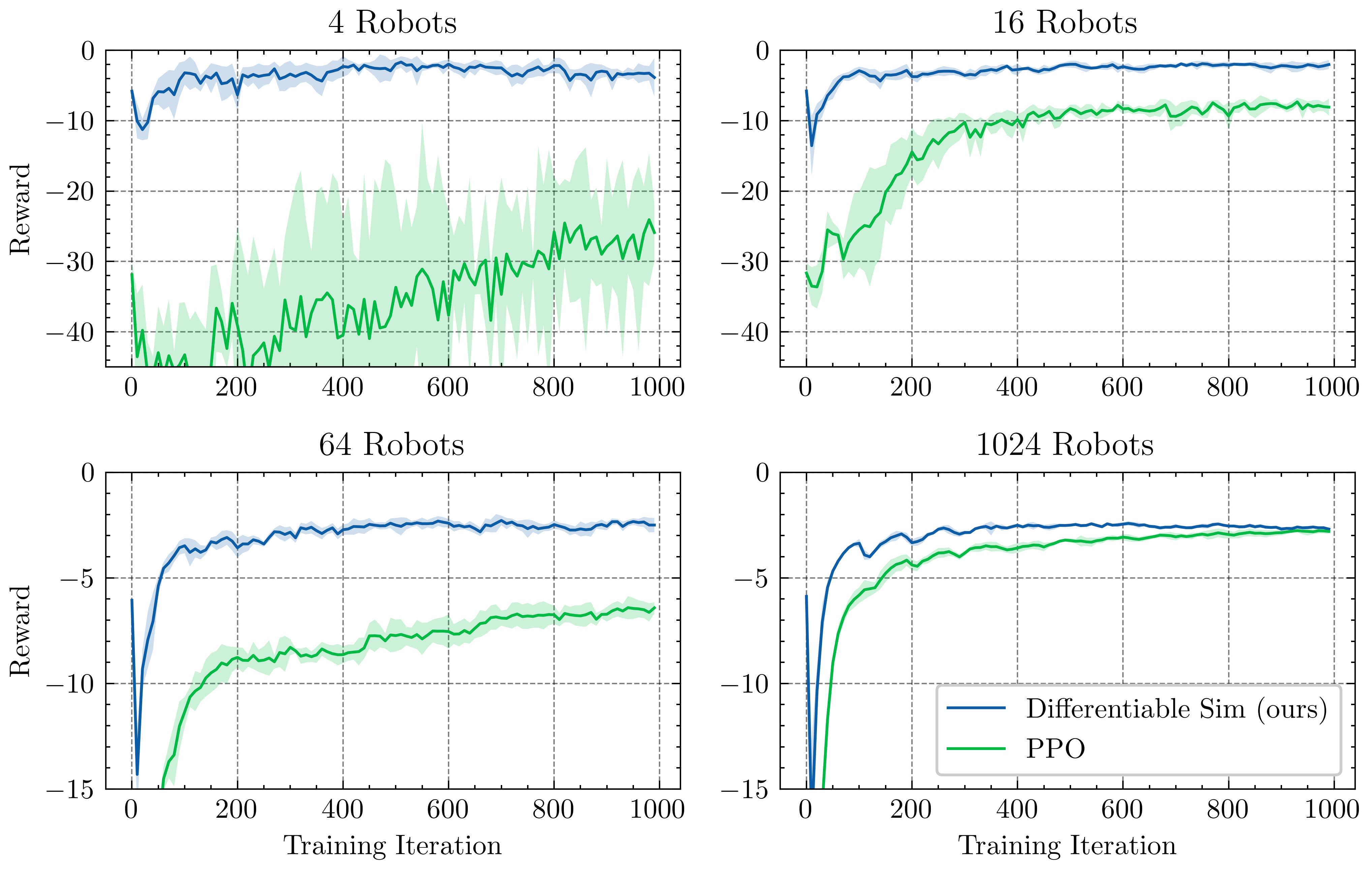
Figure 4: Learning to walk on challenging terrains, reinforcement learning versus differentiable simulation. Differentiable simulation achieves faster and more stable convergence, given limited simulation samples.

Additionally, we compare the training wall-clock time and the performance of the resulting policies between the two methodologies. Differentiable simulation often involves the creation of a complex computational graph to facilitate gradient computation, especially for backpropagation through time. As the simulation horizon extends, the length of the computational graph can increase proportionally, leading to a substantial increase in the total training time. This increase can diminish its benefits in situations where gathering a large number of samples is both cheap and fast.

Robots	Final Reward		Training Time [min]
	PPO	Ours	PPO	Ours
4	$-25.82\pm 2.16$	$\mathbf{-3.83\pm 3.01}$	$\mathbf{7.27\pm 0.12}$	$7.28\pm 0.12$
16	$-8.07\pm 1.30$	$\mathbf{-2.03\pm 0.69}$	$7.54\pm 0.06$	$\mathbf{7.50\pm 0.08}$
64	$-6.42\pm 0.29$	$\mathbf{-2.49\pm 0.37}$	$8.46\pm 0.16$	$\mathbf{8.23\pm 0.07}$
1024	$-2.80\pm 0.13$	$\mathbf{-2.69\pm 0.06}$	$\mathbf{11.44\pm 0.13}$	$11.55\pm 0.09$

TABLE II: Learning to walk on challenging terrains, reinforcement learning versus differentiable control. We compare the final reward and the total training walk-clock time.

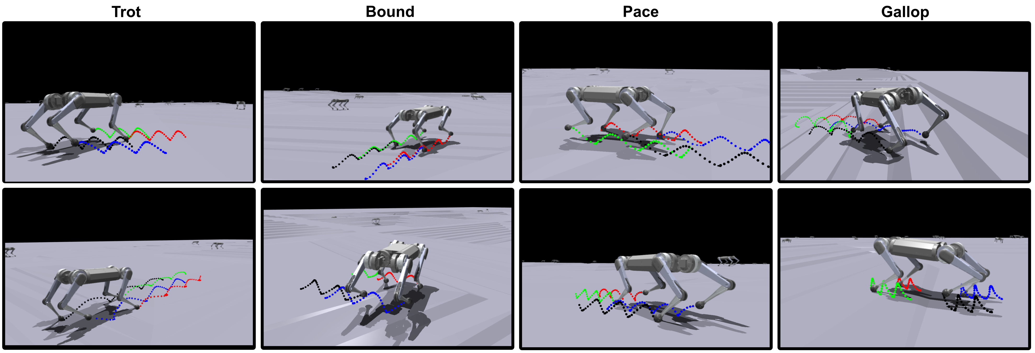
Figure 5: Diverse locomotion skills over challenging terrains using a blind policy trained via differentiable simulation.

As presented in Table II, a differentiable simulation achieves comparable overall training time. This efficiency is achieved by employing a truncated simulation timestep, which results in a smaller computational graph and enables fast and effective backpropagation. RL requires marginally longer training time due to its mini-batch and multi-epoch training scheme, in contrast, differentiable simulation only uses one gradient update. Differentiable simulation achieved overall higher reward during evaluation.

V-C On the Importance of Non-differentiable Terminal Penalty

This subsection highlights one important benefit of Reinforcement Learning (RL) compared to differentiable simulation: RL can significantly enhance its robustness by directly optimizing through non-differentiable rewards or penalties. Specifically, we use an non-differentiable value $p=200$ to penalize the robot (Eq. 7) when the robot experiences termination during training, e.g., falling on the ground.

$$r(\mathbf{x}_{t},\mathbf{u}_{t})=\begin{cases}-l(\mathbf{x}_{t},\mathbf{u}_{t})-p&\text{if termination}\\ -l(\mathbf{x}_{t},\mathbf{u}_{t})&\text{otherwise}\end{cases}$$ (8)

Fig. 6 shows a study of using non-differentiable terminal penalty for both RL and differentiable simulation. The results show that adding a final penalty can greatly affect how well reinforcement learning (RL) works. Without a penalty, RL might get trapped in a local minimum. However, with a large penalty at the end, RL can achieve better task reward as well as more robust control performance. This is because RL optimizes a discounted return, which estimates “how good” it is to be in a given state. RL uses a state-value function to encode this information

$$V_{\pi}(s)=\mathbb{E}[G|S_{0}=s]=\mathbb{E}\left[\sum_{t=0}^{\infty}\gamma^{t}R_{t+1}|S_{0}=s\right],$$ (9)

On the other hand, a terminal penalty has no impact on differentiable simulation since the gradient of a constant value is equal to zero. As a result, differentiable simulation requires well-defined continuous functions, e.g., a potential function or control barrier functions for robust control.

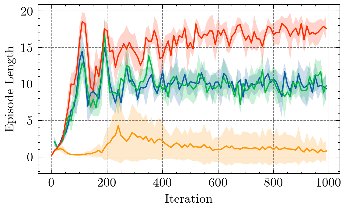
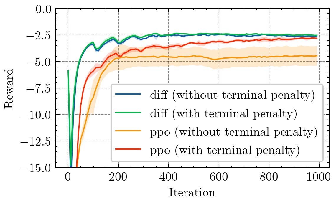
Figure 6: A comparison of non-differentiable terminal penalty for policy training. Using a non-differentiable terminal penalty, PPO can achieve robust control performance, e.g., longer episode length. We use 1024 robots for simulation.

V-D Real World Experiment

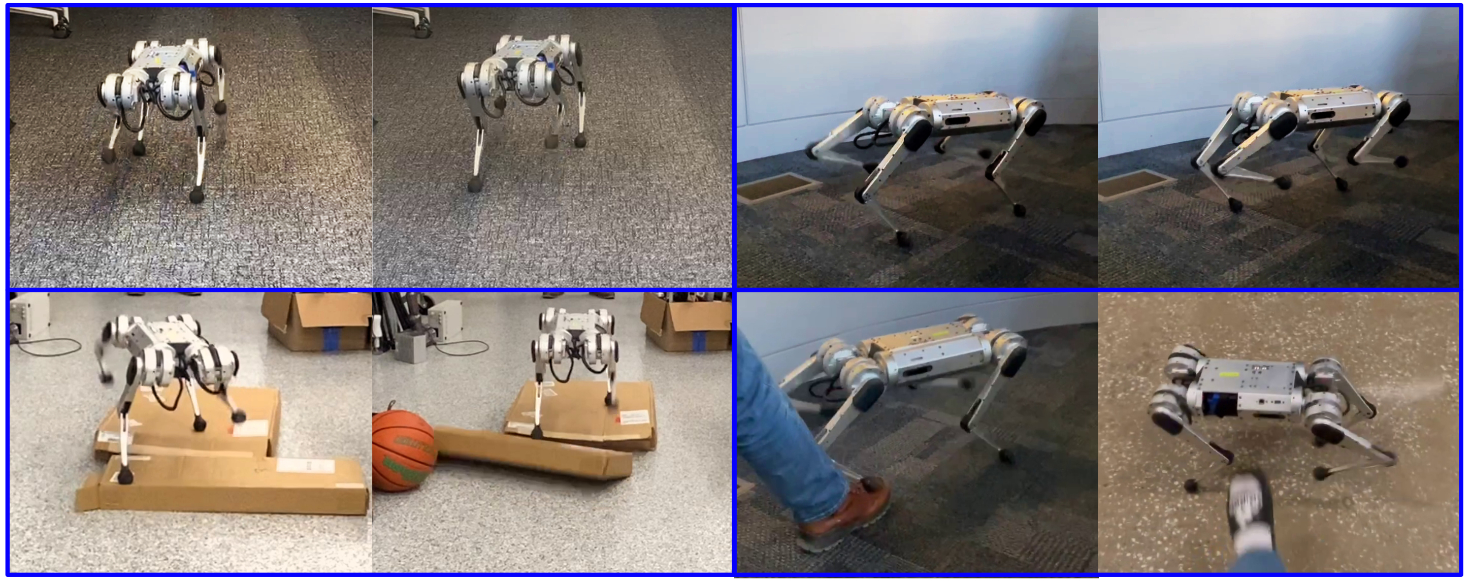
Figure 7: Real-world deployment using a Mini Cheetah. All the experiments are conducted using one single blind policy.

We demonstrate the performance of our policy in the real world using Mini Cheetah. Fig. 7 shows several snapshots of the robot’s behavior using different gait patterns. We trained a blind policy in simulation using 64 robots and then transfer the policy directly to the real world without fine-tuning. The robot can walk forward and backward with different gait patterns and frequencies. Moreover, the policy proved robust, enabling the robot to manage certain disruptions, such as unexpected forces applied to its body and locomotion on deformable terrain.

VI Limitations

A fundamental advantage of reinforcement learning (zeroth-order gradient optimization) lies in its optimization objective: RL can directly optimize non-differentiable rewards, including task-level rewards [32]. Conversely, differential simulation relies on information to be backpropagated from its differentiable loss function, making it challenging to explore novel solutions guided by task-level objectives, e.g., how to make survive differentiable?

Our system design requires the specification of foot position using heuristic methods, which is a limitation compared to RL. RL’s flexibility allows for more robust performance enhancements, such as implementing a simple termination penalty to discourage falling behaviors or employing constant survival rewards to promote longevity.

VII Conclusion

In conclusion, we propose a novel framework leveraging the advantages of differentiable simulators for the complex task of quadruped locomotion in the real world. Our framework overcomes the challenges of contact-rich environments for differentiable simulators by integrating a simplified rigid-body model with a non-differentiable model for whole-body dynamics. In this setting, the learned locomotion policy is updated by directly backpropagating the differentiable loss function through the simplified model while the state of the robot is aligned using the more precise whole-body dynamics model. This framework not only introduces the advantages of faster and more stable training convergence of differential simulators to legged robots but also ensures the accurate simulation of complex contact forces. Notably, our experiments demonstrate that the proposed framework can train a policy to walk in minutes using only one simulation environment, a setting in which model-free RL falls short. Furthermore, the policy, aligned with an accurate simulator, seamlessly transfers to the real world in a zero-shot fashion.

An interesting future application of our simulator alignment is the task of learning directly on the hardware, where the locomotion policy is continually updated using the differentiable model in an online fashion while aligning robot states directly with real-world states. Beyond this, the proven training stability and fast training convergence of our differential simulator framework holds the promise for addressing the high-sample inefficiency in tasks like vision-based policy for navigation. In summary, our work bridges the gap between differentiable simulators and real-world legged locomotion, opening avenues for numerous future applications.

VIII Acknowledgments

This work was supported by the European Union’s Horizon Europe Research and Innovation Programme under grant agreement No. 101120732 (AUTOASSESS) and the European Research Council (ERC) under grant agreement No. 864042 (AGILEFLIGHT). The authors especially thank Yuang Zhang for his help with the software development, Seungwoo Hong for the useful discussion about rigid-body dynamics and nonlinear model predictive control, and Nico Messikommer for the valuable feedback. Also, the authors thank Se Hwan Jeon, Ho Jae Lee, Matthew Chignoli, Steve Heim, Elijah Stanger-Jones, and Charles Khazoom for their helpful support.

References

- Agarwal et al. [2023] Ananye Agarwal, Ashish Kumar, Jitendra Malik, and Deepak Pathak. Legged locomotion in challenging terrains using egocentric vision. In Conference on Robot Learning, pages 403–415. PMLR, 2023.
- Bledt and Kim [2019] Gerardo Bledt and Sangbae Kim. Implementing regularized predictive control for simultaneous real-time footstep and ground reaction force optimization. In 2019 IEEE/RSJ International Conference on Intelligent Robots and Systems (IROS), pages 6316–6323. IEEE, 2019.
- Bradbury et al. [2018] James Bradbury, Roy Frostig, Peter Hawkins, Matthew James Johnson, Chris Leary, Dougal Maclaurin, George Necula, Adam Paszke, Jake VanderPlas, Skye Wanderman-Milne, and Qiao Zhang. JAX: composable transformations of Python+NumPy programs, 2018. URL http://github.com/google/jax.
- Chen et al. [2020] Dian Chen, Brady Zhou, Vladlen Koltun, and Philipp Krähenbühl. Learning by cheating. In Conference on Robot Learning, pages 66–75. PMLR, 2020.
- de Avila Belbute-Peres et al. [2018] Filipe de Avila Belbute-Peres, Kevin Smith, Kelsey Allen, Josh Tenenbaum, and J Zico Kolter. End-to-end differentiable physics for learning and control. Advances in neural information processing systems, 31, 2018.
- Deisenroth et al. [2013] Marc Peter Deisenroth, Gerhard Neumann, Jan Peters, et al. A survey on policy search for robotics. Foundations and Trends® in Robotics, 2(1–2):1–142, 2013.
- Di Carlo et al. [2018] Jared Di Carlo, Patrick M Wensing, Benjamin Katz, Gerardo Bledt, and Sangbae Kim. Dynamic locomotion in the mit cheetah 3 through convex model-predictive control. In 2018 IEEE/RSJ international conference on intelligent robots and systems (IROS), pages 1–9. IEEE, 2018.
- Freeman et al. [2021] C Daniel Freeman, Erik Frey, Anton Raichuk, Sertan Girgin, Igor Mordatch, and Olivier Bachem. Brax–a differentiable physics engine for large scale rigid body simulation. arXiv preprint arXiv:2106.13281, 2021.
- Fu et al. [2023] Zipeng Fu, Xuxin Cheng, and Deepak Pathak. Deep whole-body control: learning a unified policy for manipulation and locomotion. In Conference on Robot Learning, pages 138–149. PMLR, 2023.
- Grandia et al. [2023] Ruben Grandia, Fabian Jenelten, Shaohui Yang, Farbod Farshidian, and Marco Hutter. Perceptive locomotion through nonlinear model-predictive control. IEEE Transactions on Robotics, 2023.
- Hong et al. [2020] Seungwoo Hong, Joon-Ha Kim, and Hae-Won Park. Real-time constrained nonlinear model predictive control on so (3) for dynamic legged locomotion. In 2020 IEEE/RSJ International Conference on Intelligent Robots and Systems (IROS), pages 3982–3989. IEEE, 2020.
- Howell et al. [2022] Taylor Howell, Simon Le Cleac’h, Jan Bruedigam, Zico Kolter, Mac Schwager, and Zachary Manchester. Dojo: A differentiable simulator for robotics. arXiv preprint arXiv:2203.00806, 2022. URL https://arxiv.org/abs/2203.00806.
- Hu et al. [2019] Yuanming Hu, Luke Anderson, Tzu-Mao Li, Qi Sun, Nathan Carr, Jonathan Ragan-Kelley, and Frédo Durand. Difftaichi: Differentiable programming for physical simulation. arXiv preprint arXiv:1910.00935, 2019.
- Huang et al. [2021] Zhiao Huang, Yuanming Hu, Tao Du, Siyuan Zhou, Hao Su, Joshua B Tenenbaum, and Chuang Gan. Plasticinelab: A soft-body manipulation benchmark with differentiable physics. arXiv preprint arXiv:2104.03311, 2021.
- Hwangbo et al. [2019] Jemin Hwangbo, Joonho Lee, Alexey Dosovitskiy, Dario Bellicoso, Vassilios Tsounis, Vladlen Koltun, and Marco Hutter. Learning agile and dynamic motor skills for legged robots. Science Robotics, 4(26):eaau5872, 2019.
- Kalakrishnan et al. [2010] Mrinal Kalakrishnan, Jonas Buchli, Peter Pastor, Michael Mistry, and Stefan Schaal. Fast, robust quadruped locomotion over challenging terrain. In 2010 IEEE International Conference on Robotics and Automation, pages 2665–2670. IEEE, 2010.
- Katz et al. [2019] Benjamin Katz, Jared Di Carlo, and Sangbae Kim. Mini cheetah: A platform for pushing the limits of dynamic quadruped control. In 2019 International Conference on Robotics and Automation (ICRA), pages 6295–6301, 2019. doi: 10.1109/ICRA.2019.8793865.
- Kolter et al. [2008] J Zico Kolter, Mike P Rodgers, and Andrew Y Ng. A control architecture for quadruped locomotion over rough terrain. In 2008 IEEE International Conference on Robotics and Automation, pages 811–818. IEEE, 2008.
- Kumar et al. [2021] Ashish Kumar, Zipeng Fu, Deepak Pathak, and Jitendra Malik. Rma: Rapid motor adaptation for legged robots. arXiv preprint arXiv:2107.04034, 2021.
- Lee et al. [2020] Joonho Lee, Jemin Hwangbo, Lorenz Wellhausen, Vladlen Koltun, and Marco Hutter. Learning quadrupedal locomotion over challenging terrain. Science robotics, 5(47):eabc5986, 2020.
- Makoviychuk et al. [2021] Viktor Makoviychuk, Lukasz Wawrzyniak, Yunrong Guo, Michelle Lu, Kier Storey, Miles Macklin, David Hoeller, Nikita Rudin, Arthur Allshire, Ankur Handa, and Gavriel State. Isaac gym: High performance gpu-based physics simulation for robot learning, 2021.
- Margolis et al. [2022] Gabriel B Margolis, Ge Yang, Kartik Paigwar, Tao Chen, and Pulkit Agrawal. Rapid locomotion via reinforcement learning. arXiv preprint arXiv:2205.02824, 2022.
- Metz et al. [2021] Luke Metz, C Daniel Freeman, Samuel S Schoenholz, and Tal Kachman. Gradients are not all you need. arXiv preprint arXiv:2111.05803, 2021.
- Miki et al. [2022] Takahiro Miki, Joonho Lee, Jemin Hwangbo, Lorenz Wellhausen, Vladlen Koltun, and Marco Hutter. Learning robust perceptive locomotion for quadrupedal robots in the wild. Science Robotics, 7(62):eabk2822, 2022.
- Mora et al. [2021] Miguel Angel Zamora Mora, Momchil Peychev, Sehoon Ha, Martin Vechev, and Stelian Coros. Pods: Policy optimization via differentiable simulation. In International Conference on Machine Learning, pages 7805–7817. PMLR, 2021.
- Neunert et al. [2018] Michael Neunert, Markus Stäuble, Markus Giftthaler, Carmine D Bellicoso, Jan Carius, Christian Gehring, Marco Hutter, and Jonas Buchli. Whole-body nonlinear model predictive control through contacts for quadrupeds. IEEE Robotics and Automation Letters, 3(3):1458–1465, 2018.
- Paszke et al. [2019] Adam Paszke, Sam Gross, Francisco Massa, Adam Lerer, James Bradbury, Gregory Chanan, Trevor Killeen, Zeming Lin, Natalia Gimelshein, Luca Antiga, et al. Pytorch: An imperative style, high-performance deep learning library. Advances in neural information processing systems, 32, 2019.
- Raibert [1986] Marc H Raibert. Legged robots that balance. MIT press, 1986.
- Ren et al. [2023] Jiawei Ren, Cunjun Yu, Siwei Chen, Xiao Ma, Liang Pan, and Ziwei Liu. Diffmimic: Efficient motion mimicking with differentiable physics. 2023.
- Rudin et al. [2022] Nikita Rudin, David Hoeller, Philipp Reist, and Marco Hutter. Learning to walk in minutes using massively parallel deep reinforcement learning. In Conference on Robot Learning, pages 91–100. PMLR, 2022.
- Schulman et al. [2017] John Schulman, Filip Wolski, Prafulla Dhariwal, Alec Radford, and Oleg Klimov. Proximal policy optimization algorithms. arXiv preprint arXiv:1707.06347, 2017.
- Song et al. [2023] Yunlong Song, Angel Romero, Matthias Müller, Vladlen Koltun, and Davide Scaramuzza. Reaching the limit in autonomous racing: Optimal control versus reinforcement learning. Science Robotics, 8(82):eadg1462, 2023.
- Suh et al. [2022] Hyung Ju Suh, Max Simchowitz, Kaiqing Zhang, and Russ Tedrake. Do differentiable simulators give better policy gradients? In International Conference on Machine Learning, pages 20668–20696. PMLR, 2022.
- Sutton and Barto [2018] Richard S Sutton and Andrew G Barto. Reinforcement learning: An introduction. MIT press, 2018.
- Williams [1992] Ronald J Williams. Simple statistical gradient-following algorithms for connectionist reinforcement learning. Machine learning, 8:229–256, 1992.
- Xu et al. [2021] Jie Xu, Viktor Makoviychuk, Yashraj Narang, Fabio Ramos, Wojciech Matusik, Animesh Garg, and Miles Macklin. Accelerated policy learning with parallel differentiable simulation. In International Conference on Learning Representations, 2021.
- Xu et al. [2022] Jie Xu, Sangwoon Kim, Tao Chen, Alberto Rodriguez Garcia, Pulkit Agrawal, Wojciech Matusik, and Shinjiro Sueda. Efficient tactile simulation with differentiability for robotic manipulation. In 6th Annual Conference on Robot Learning, 2022. URL https://openreview.net/forum?id=6BIffCl6gsM.
- Yang et al. [2023] Yuxiang Yang, Guanya Shi, Xiangyun Meng, Wenhao Yu, Tingnan Zhang, Jie Tan, and Byron Boots. Cajun: Continuous adaptive jumping using a learned centroidal controller. arXiv preprint arXiv:2306.09557, 2023.
- Zhuang et al. [2023] Ziwen Zhuang, Zipeng Fu, Jianren Wang, Christopher Atkeson, Soeren Schwertfeger, Chelsea Finn, and Hang Zhao. Robot parkour learning. arXiv preprint arXiv:2309.05665, 2023.