Learning WENO for entropy stable schemes to solve conservation laws

Abstract

Entropy conditions play a crucial role in the extraction of a physically relevant solution for a system of conservation laws, thus motivating the construction of entropy stable schemes that satisfy a discrete analogue of such conditions. TeCNO schemes (Fjordholm et al. 2012) [14] form a class of arbitrary high-order entropy stable finite difference solvers, which require specialized reconstruction algorithms satisfying the sign property at each cell interface. Recently, third-order WENO schemes called SP-WENO (Fjordholm and Ray, 2016) [16] and SP-WENOc (Ray, 2018) [44] have been designed to satisfy the sign property. However, these WENO algorithms can perform poorly near shocks, with the numerical solutions exhibiting large spurious oscillations. In the present work, we propose a variant of the SP-WENO, termed as Deep Sign-Preserving WENO (DSP-WENO), where a neural network is trained to learn the WENO weighting strategy. The sign property and third-order accuracy are strongly imposed in the algorithm, which constrains the WENO weight selection region to a convex polygon. Thereafter, a neural network is trained to select the WENO weights from this convex region with the goal of improving the shock-capturing capabilities without sacrificing the rate of convergence in smooth regions. The proposed synergistic approach retains the mathematical framework of the TeCNO scheme while integrating deep learning to remedy the computational issues of the WENO-based reconstruction. We present several numerical experiments to demonstrate the significant improvement with DSP-WENO over the existing variants of WENO satisfying the sign property.

1 Introduction

Hyperbolic systems of conservation laws dictate the behavior of quantities that are conserved in time as the system evolves. These systems of PDEs are ubiquitous across many disciplines. A generic system of conservation laws in one spatial dimension can be mathematically expressed as

$$\frac{\partial}{\partial t}{\bm{u}}(x,t)+\frac{\partial}{\partial x}{\bm{f}}({\bm{u}}(x,t)) =\mathbf{0}\quad \forall\ x\in\Omega\subset\mathbb{R},\ t\in\mathbb{R}^{+}$$ (1)

$${\bm{u}}(x,0) ={\bm{u}}_{0}(x)\quad \forall\ x\in\Omega,$$

where ${\bm{u}}$: $\Omega\times\mathbb{R}^{+}\xrightarrow{}\mathbb{R}^{d}$ represents a vector of $d$ conserved variables and ${\bm{f}}$: $\mathbb{R}^{d}\xrightarrow{}\mathbb{R}^{d}$ is a smooth flux, representing the flow of the conserved quantities.

However, it is well-known that solutions to nonlinear conservation laws can develop discontinuities in finite time even with smooth initial conditions. Thus, solutions to (1) must be understood in the weak (distributional) sense. Moreover, since weak solutions are not unique in general, additional constraints in terms of the entropy conditions must be imposed such that a physically relevant weak solution is extracted. Assume that for (1), $\eta({\bm{u}})$ is a convex entropy function and $q({\bm{u}})$ is the entropy flux function satisfying the compatibility condition

$$\nabla_{{\bm{u}}}q({\bm{u}})^{\top}=\nabla_{{\bm{u}}}\eta({\bm{u}})^{\top}\nabla_{\bm{u}}{\bm{f}}({\bm{u}}).$$

The solution ${\bm{u}}$ of (1) is said to be an entropy solution if it satisfies the following inequality for all admissible entropy pairs $(\eta({\bm{u}}),q({\bm{u}}))$ associated with (1):

$$\frac{\partial}{\partial t}\eta({\bm{u}})+\frac{\partial}{\partial x}q({\bm{u}})\leq 0,$$ (2)

which is understood in the weak sense. The entropy is conserved for smooth solutions, and thus (2) is taken to be an equality, i.e., $\eta$ is the solution of a conservation law. In contrast, entropy is dissipated near shocks, thus the inequality in (2) is strict near such discontinuities. Scalar conservation laws have unique entropy solutions [27], but the uniqueness of entropy solutions is not guaranteed for general systems of conservation laws [31, 8]. However, the entropy conditions provide the only non-linear estimates currently available for generic systems of conservation laws [10], and are thus essential. In practice, the entropy condition (2) is considered with respect to a specific choice of $(\eta({\bm{u}}),q({\bm{u}}))$ for a general system (1).

It is meaningful to develop entropy stables scheme, i.e., schemes satisfying a discrete version of (2), to solve systems of conservation laws. Further, it is essential for such methods to be high-order accurate while being capable of capturing discontinuities without spurious oscillations. There has been much focus on this area in the past few decades, and finite difference methods remain one such popular framework. In finite difference methods, the computational domain is partitioned into cells, on which a discrete version of the conservation law is formulated. Point values of the solution in the cells are evolved in time using time integration techniques, such as strong stability preserving Runge-Kutta methods [18]. In [53], a novel approach to constructing entropy stable finite difference schemes was proposed, which comprises two steps: (1) beginning with a second-order entropy conservative flux such that entropy is conserved locally and (2) adding an artificial dissipation term to ensure entropy stability.

TeCNO schemes [14] are a popular class of arbitrary high-order entropy stable finite difference schemes which build on the formulation considered in [53]. These schemes consist of augmenting high-order entropy conservative fluxes with high-order numerical diffusion, which rely on specialized polynomial reconstruction algorithms. Crucially, these reconstructions must satisfy a sign property at each cell interface so that entropy stability is ensured. This property requires the jump in the reconstructed cell interface values to have the same sign as the jump in the corresponding cell values.

Although any reconstruction method with the sign property can be used to formulate entropy stable TeCNO schemes, only a handful of such algorithms are currently available. The second-order limited total variation diminishing (TVD) using the minmod limiter is the simplest reconstruction possessing the sign property [14]. Third-order and fourth-order sign-preserving reconstructions based on non-linear limiting of polynomials were proposed [7, 6]. The essentially non-oscillatory (ENO) reconstruction method, which adaptively chooses the smoothest stencil for reconstruction, satisfies the sign property as demonstrated in [15]. To overcome some of the computational challenges encountered when using ENO, third-order weighted ENO (WENO) reconstructions were proposed in [16, 44] which guarantee the sign property. However, these WENO schemes (termed as SP-WENO), while ensuring entropy stability in the TeCNO framework, are susceptible to spurious oscillations near discontinuities. We will highlight this issue in greater detail in the present work. We also mention here an alternate strategy [39] based on TeCNO schemes, where the sign property of reconstructions is not required. Instead, a specialized diffusion operator is constructed to ensure entropy stability, which can be used with any high-order reconstruction algorithm. We will not focus on this approach in the present work.

The last few years have witnessed a surge in the use of deep learning-based strategies to solve problems in scientific computing. Key examples includes building surrogates to solve PDEs [43, 9, 35, 33, 40], learning parameter-to-observable maps [37, 36, 21], solving Bayesian inference problems [17, 41, 56, 11, 47], or learning closure models [51, 2, 38]. Among these is the class of deep learning (DL) approaches which aim to enhance existing numerical solvers, instead of replacing them. The philosophy here is to first identify computational bottlenecks in the solver, and then use domain knowledge to train specialized neural networks to replace the bottleneck, keeping the rest of the solver intact. Thus, this synergistic approach leverages the “best of both worlds”, leading to a more robust numerical solver aided by DL. For instance, in [45, 46], deep-learned troubled-cell indicators were designed for discontinuous Galerkin (DG) schemes solving conservation laws, to identify (classify) elements containing discontinuities. Once flagged, the DG solver can apply any suitable limiter in the troubled-cells to avoid Gibbs oscillations. These DL indicators are free of problem-dependent parameters and trained in model agnostic manner, i.e., the same network can be used to solve any system of conservation laws. Similar DL-based shock capturing strategies have also been explored in [13, 3, 58, 49, 4, 1]

DL techniques have also been used to learn ENO/WENO-type reconstructions. In [12], it was shown that ENO (and some of its variants) are equivalent to deep ReLU neural networks, which in turn highlighted the potential of deep networks to approximate rough functions. A six-point ENO-type reconstruction was proposed in [32] where the stencil selection is performed using a neural network. However, when used to solve conservation laws, some numerical experiments were accompanied by a degeneracy in the expected order of accuracy. In [52], a neural network was trained to develop an optimal variant of the classical WENO-JS [23]. The trained network, called WENO-NN, was shown to outperform WENO-JS by being for anti-diffusive leading to sharper shock profiles in numerical solutions. However, this also lead to the development of spurious oscillations in under-resolved simulations. Further, WENO-NN was not able to retain the desired order of accuracy for smooth solutions. A DL-based fifth-order WENO called WENO-DS was proposed in [26], where the WENO weights were fine-tuned to improve its shock-capturing capabilities. The authors proved the formal order of accuracy of WENO-DS, and also demonstrated it numerically. However, WENO-DS is trained using the flux values as input to the network, thus it is designed to work for a specific conservation law model. The network is tuned separately for each PDE considered, and thus, one instance of WENO-DS is not generally model agnostic.

In the present work, we are interested in using DL to recover reconstruction algorithms constrained to satisfy useful physical properties. In particular, we construct a variant of SP-WENO, which we call DSP-WENO, where a neural network predicts the weights associated with the reconstruction, while ensuring that the sign property (along with other crucial constraints) are satisfied. These constraints are strongly imposed which results in a convex polygonal region for the WENO weight selection. Then, a neural network is trained on suitably generated training samples to learn the weight selection algorithm of the DSP-WENO for appropriate behavior near discontinuities and smooth regions. The proposed DSP-WENO is constructed to be third-order accurate, which is also demonstrated numerically. When used in the TeCNO framework, DSP-WENO overcomes the computational issues faced by the existing SP-WENO strategies. We re-iterate that the DSP-WENO only replaces the reconstruction needed in the high-order diffusion term, keeping the rest of the TeCNO framework intact. Thus the proposed method can be seen as a deep learning-based enhancement of an existing numerical algorithm. We remark here that a single DSP-WENO network is trained (offline) to be used with any conservation laws, i.e., the proposed algorithm is agnostic to the specific PDE model being solved.

The rest of the paper is organized as follows. In Section 2, we describe the framework of high-order entropy stable finite difference schemes. In Section 3, we introduce the formulation and properties of existing sign-preserving WENO reconstructions. The construction of our DL-based method is explained in Section 4. The results of various numerical tests including one-dimensional and two-dimensional scalar and systems of conservation laws are presented in Section 5. Final conclusions and future directions are discussed in Section 6.

2 Finite Difference Schemes/Entropy Stable Schemes

We consider a one-dimensional finite difference formulation for ease of discussion, which can easily be extended to higher dimensions. We partition the spatial domain $\Omega$ using disjoint cells $I_{i}=[x_{i-\frac{1}{2}},x_{i+\frac{1}{2}})$ of uniform length $h\equiv x_{i+\frac{1}{2}}-x_{i-\frac{1}{2}}$. The mesh point $x_{i}$ is the center of the cell $I_{i}$ while the half indices denote the cell interfaces. Figure 1 shows an example of the discretized mesh. Keeping time continuous, the semi-discrete finite difference scheme for (1) is expressed as

$$\frac{d{\bm{u}}_{i}(t)}{dt}+\frac{1}{h}({\bm{f}}_{i+\frac{1}{2}}-{\bm{f}}_{i-\frac{1}{2}})=0.$$ (3)

Here, ${\bm{u}}_{i}(t)$ approximates the point values of the solution to (1) at cell center $x_{i}$ and time $t$, while ${\bm{f}}_{i+\frac{1}{2}}$ is a consistent, conservative numerical approximation of the flux ${\bm{f}}$ at the cell interface $x_{i+\frac{1}{2}}$. We seek entropy stable schemes to approximate (1) which satisfy a discrete version of the entropy condition (2). As described in [53], we begin by constructing an entropy conservative scheme.

Definition 1.

The numerical scheme (3) is entropy conservative if it satisfies the following discretization of (2)

$$\frac{d\eta({\bm{u}}_{i})}{dt}+\frac{1}{h}\left(\tilde{q}_{i+\frac{1}{2}}-\tilde{q}_{i-\frac{1}{2}}\right)=0,$$ (4)

where $\tilde{q}_{i+\frac{1}{2}}$ is a numerical entropy flux consistent with entropy flux $q$ in (2).

Figure 1: The mesh for finite difference schemes. Cell centers are labeled as integers, and the interfaces or cell boundaries are labeled using half indices: $x_{i+\frac{1}{2}}$ is between cells $I_{i}$ and $I_{i+1}$. When reconstructing the function at an interface, we can either reconstruct from the left (as indicated in blue) or from the right (as indicated in green).

We denote the undivided jump and average across the interface $x_{i+\frac{1}{2}}$ by

$$\Delta(\cdot)_{i+\frac{1}{2}}=(\cdot)_{i+1}-(\cdot)_{i},\hskip 8.53581pt\overline{(\cdot)}_{i+\frac{1}{2}}=\frac{(\cdot)_{i+1}+(\cdot)_{i}}{2}.$$

Additionally, we introduce the entropy potential $\Psi({\bm{u}}):={\bm{v}}({\bm{u}})^{\top}{\bm{f}}({\bm{u}})-q({\bm{u}})$, where ${\bm{v}}({\bm{u}})=\nabla_{\bm{u}}\eta({\bm{u}})$ is the vector of entropy variables. A sufficient condition for constructing entropy conservative fluxes is provided by the following theorem.

Theorem 1.

([53]) The second-order accurate numerical scheme (3) with the two-point numerical flux $\tilde{{\bm{f}}}_{i+\frac{1}{2}}=\tilde{{\bm{f}}}_{i+\frac{1}{2}}({\bm{u}}_{i},{\bm{u}}_{i+1})$ is entropy conservative if

$$\left(\Delta{\bm{v}}_{i+\frac{1}{2}}\right)^{\top}\tilde{{\bm{f}}}_{i+\frac{1}{2}}=\Delta\Psi_{i+\frac{1}{2}}.$$ (5)

Specifically, it satisfies the entropy condition with the consistent numerical entropy flux given by

$$\tilde{q}_{i+\frac{1}{2}}=\left(\overline{{\bm{v}}}_{i+\frac{1}{2}}\right)^{\top}\tilde{{\bm{f}}}_{i+\frac{1}{2}}-\overline{\Psi}_{i+\frac{1}{2}}.$$

The expression (5) in Theorem 1 provides a recipe to construct second-order entropy conservative fluxes. It leads to a unique flux construction for scalar conservation laws (given $\eta)$. For systems of conservation laws, it is possible to carefully construct numerical fluxes that satisfy (5) with additional desirable properties [22, 5, 55, 19]. To construct higher-order entropy conservative fluxes, we follow the approach in [30]. This involves computing suitable linear combinations of the second-order two-point fluxes

$$\tilde{{\bm{f}}}_{i+\frac{1}{2}}^{2p}=\sum_{r=1}^{p}B_{r}^{p}\sum_{s=0}^{r-1}\tilde{{\bm{f}}}({\bm{u}}_{i-s},{\bm{u}}_{i-s+r}),$$ (6)

which yields $2p$th-order accurate entropy conservative fluxes. The scalar coefficients $B_{r}^{p}$ can be obtained by solving the $p$ linear equations

$$2\sum_{r=1}^{p}rB_{r}^{p}=1,\hskip 8.53581pt\sum_{i=1}^{p}i^{2s-1}B_{r}^{p}=0\hskip 8.53581pt(s=2,...,p).$$

For example, the fourth-order entropy conservative flux is given by

$$\tilde{{\bm{f}}}_{i+\frac{1}{2}}^{2p}=\frac{4}{3}\tilde{{\bm{f}}}({\bm{u}}_{i},{\bm{u}}_{i+1})-\frac{1}{6}\left(\tilde{{\bm{f}}}({\bm{u}}_{i-1},{\bm{u}}_{i+1})+\tilde{{\bm{f}}}({\bm{u}}_{i},{\bm{u}}_{i+2})\right).$$ (7)

Entropy is conserved for smooth solutions and thus using an entropy conservative scheme is meaningful. However, entropy is dissipated near discontinuities in accordance to (2). Hence, an entropy variable-based numerical dissipation term is added to the entropy conservative numerical flux

$${\bm{f}}_{i+\frac{1}{2}}=\tilde{{\bm{f}}}^{2p}_{i+\frac{1}{2}}-\frac{1}{2}\mathbf{D}_{i+\frac{1}{2}}\Delta{\bm{v}}_{i+\frac{1}{2}},$$ (8)

where $\mathbf{D}_{i+\frac{1}{2}}\succeq 0$ (a positive semi-definite matrix) is evaluated at some suitable averaged states. The numerical flux (8) satisfies the following result.

Lemma 1.

([14]) The numerical scheme (3) with numerical flux (8) satisfies the discrete entropy inequality

$$\frac{d\eta({\bm{u}}_{i})}{dt}+\frac{1}{h}\left(q_{i+\frac{1}{2}}-q_{i-\frac{1}{2}}\right)\leq 0,$$ (9)

where the numerical entropy flux is of the form

$$q_{i+\frac{1}{2}}=\tilde{q}_{i+\frac{1}{2}}-\frac{1}{2}\left(\overline{{\bm{v}}}_{i+\frac{1}{2}}\right)^{\top}\mathbf{D}_{i+\frac{1}{2}}\Delta{\bm{v}}_{i+\frac{1}{2}}.$$ (10)

While any positive semi-definite matrix ensures entropy stability in the sense of (9), we choose the form $\mathbf{D}_{i+\frac{1}{2}}=\mathbf{R}_{i+\frac{1}{2}}\Lambda_{i+\frac{1}{2}}\mathbf{R}^{\top}_{i+\frac{1}{2}}$. Here, $\mathbf{R}$ is a matrix consisting of the right eigenvectors of the flux Jacobian and $\mathbf{\Lambda}$ is a nonnegative diagonal matrix that depends on the eigenvalues of the flux Jacobian. Specifically, we choose the Roe-type diffusion matrix with $\mathbf{\Lambda}=\operatorname{diag}{(|\lambda^{1}|,...,|\lambda^{d}|)}$. See [53] for other choices for the diffusion matrix.

Note that the term $\Delta{\bm{v}}_{i+\frac{1}{2}}$ in (8) is $\mathcal{O}(h)$. Therefore, the numerical scheme that results from using (8) is only first-order accurate regardless of the accuracy of the entropy conservative flux. Since the accuracy of the scheme is limited by the diffusion term, we construct a higher-order diffusion term by suitably reconstructing the jump in entropy variables at the cell interfaces.

We consider the interface at $x_{i+\frac{1}{2}}$ between the cells $I_{i}$ and $I_{i+1}$, as shown in Figure 1. We reconstruct from the left and right of this interface. We define the (locally) scaled entropy variables ${\bm{z}}=\mathbf{R}^{\top}_{i+\frac{1}{2}}{\bm{v}}$ corresponding to this interface. The flux in (8) can thus be expressed as

$${\bm{f}}_{i+\frac{1}{2}}=\tilde{{\bm{f}}}^{2p}_{i+\frac{1}{2}}-\frac{1}{2}\mathbf{R}_{i+\frac{1}{2}}\Lambda_{i+\frac{1}{2}}\Delta{\bm{z}}_{i+\frac{1}{2}}.$$ (11)

Let ${\bm{z}}_{i}(x)$ and ${\bm{z}}_{i+1}(x)$ be polynomial reconstructions of the scaled entropy variables in $I_{i}$ and $I_{i+1}$, respectively. We denote the reconstructed values and jump at the cell interface by

$${\bm{z}}_{i+\frac{1}{2}}^{-}={\bm{z}}_{i}(x_{i+\frac{1}{2}}),\hskip 5.69054pt{\bm{z}}_{i+\frac{1}{2}}^{+}={\bm{z}}_{i+1}(x_{i+\frac{1}{2}}),\hskip 5.69054pt\llbracket{\bm{z}}\rrbracket_{i+\frac{1}{2}}={\bm{z}}_{i+\frac{1}{2}}^{+}-{\bm{z}}_{i+\frac{1}{2}}^{-}.$$

Replacing the original jump $\Delta{\bm{z}}_{i+\frac{1}{2}}$ in (11) by the reconstructed jump $\llbracket{\bm{z}}\rrbracket_{i+\frac{1}{2}}$ will lead to a higher-order accurate scheme. However, this scheme is not guaranteed to be entropy stable. The following lemma provides a sufficient condition on the reconstruction algorithm that ensures entropy stability.

Lemma 2.

([14]) For each interface $x_{i+\frac{1}{2}}$, if the reconstruction satisfies the sign property

$$\operatorname{sign}{(\llbracket{\bm{z}}\rrbracket_{i+\frac{1}{2}})}=\operatorname{sign}{(\Delta{\bm{z}}_{i+\frac{1}{2}})},$$ (12)

then the scheme with the numerical flux

$${\bm{f}}_{i+\frac{1}{2}}=\tilde{{\bm{f}}}^{2p}_{i+\frac{1}{2}}-\frac{1}{2}\mathbf{R}_{i+\frac{1}{2}}\Lambda_{i+\frac{1}{2}}\llbracket{\bm{z}}\rrbracket_{i+\frac{1}{2}},$$ (13)

is entropy stable.

High-order entropy stable schemes described in Lemma 2 are called TeCNO schemes, which rely on reconstructions satisfying the sign property (12). However, only a handful of reconstructions are known to satisfy the sign property. In [15], it was proven that ENO reconstructions satisfy this critical condition. In [16], third-order WENO schemes (known as SP-WENO) were designed to possess the sign property, which serves as the starting point for the novel reconstruction proposed in the present work. We discuss the SP-WENO formulation in Section 3.1.

3 Sign-Preserving WENO Reconstructions

A typical WENO reconstruction [23] produces a $(2k-1)$th-order accurate reconstruction by taking a convex combination of the $2k-1$ candidate polynomials considered in the $k$th-order ENO reconstruction. A third-order WENO has the following form for the left and right reconstructions of the variable $z$ at the interface $x_{i+\frac{1}{2}}$:

$$z_{i+\frac{1}{2}}^{-} =\hskip 9.95845ptw_{0,i+\frac{1}{2}}\left(\frac{z_{i}}{2}+\frac{z_{i+1}}{2}\right)+w_{1,i+\frac{1}{2}}\left(-\frac{z_{i-1}}{2}+\frac{3z_{i}}{2}\right),$$ (14)

$$z_{i+\frac{1}{2}}^{+} =\tilde{w}_{0,i+\frac{1}{2}}\left(-\frac{z_{i+2}}{2}+\frac{3z_{i+1}}{2}\right)+\tilde{w}_{1,i+\frac{1}{2}}\left(\frac{z_{i}}{2}+\frac{z_{i+1}}{2}\right),$$

where the weights must be chosen to: (i) ensure third-order accuracy of the reconstructions $z_{i+\frac{1}{2}}^{\pm}$ for smooth solutions and (ii) provide minimal weight to linear polynomials on stencils containing discontinuities. In general, WENO reconstructions do not satisfy the sign property, and their use in the TeCNO framework described by (13) does not yield entropy stable schemes. Thus, a WENO reconstruction must be specifically designed to also satisfy the sign property.

3.1 SP-WENO [16]

SP-WENO was the first variant of WENO schemes designed to satisfy the sign property. In this framework, the weights in (14) are given as

$$w_{0}=\frac{3}{4}+2C_{1},\quad\tilde{w}_{0}=\frac{1}{4}-2C_{2},\quad w_{1}=1-w_{0},\quad\tilde{w}_{1}=1-\tilde{w}_{0}.$$ (15)

We define the jump ratios at the interface $x_{i+\frac{1}{2}}$ as $\theta_{i}^{-}:=\Delta z_{i+\frac{1}{2}}/\Delta z_{i-\frac{1}{2}}$, $\theta_{i}^{+}:=1/\theta_{i}^{-}$ and the additional terms

$$\psi_{i+\frac{1}{2}}^{+}:=\frac{1-\theta_{i+1}^{-}}{1-\theta_{i}^{+}},\quad\psi_{i+\frac{1}{2}}^{-}=\frac{1}{\psi_{i+\frac{1}{2}}^{+}}.$$ (16)

Then the perturbations $C_{1}$, $C_{2}$ in SP-WENO are determined as

$$C_{1}(\theta_{i}^{+},\theta_{i+1}^{-})=\begin{cases}\frac{1}{8}\left(\frac{f^{+}}{(f^{+})^{2}+(f^{-})^{2}}\right)&\text{ if }\theta_{i}^{+}\neq 1,\psi^{+}<0,\psi^{+}\neq-1\\ 0&\text{ if }\theta_{i}^{+}\neq 1,\psi^{+}=-1\\ -\frac{3}{8}&\text{ if }\theta_{i}^{+}=1\text{ or }\psi^{+}\geq 0,|\theta_{i}^{+}|\leq 1\\ \frac{1}{8}&\text{ if }\psi^{+}\geq 0,|\theta_{i}^{+}|>1\end{cases},$$

and $C_{2}(\theta_{i}^{+},\theta_{i+1}^{-})=C_{1}(\theta_{i+1}^{-},\theta_{i}^{+})$, where

$$f^{+}(\theta_{i}^{+},\theta_{i+1}^{-}):=\begin{cases}\frac{1}{1+\psi^{+}}&\text{ if }\theta_{i}^{+}\neq 1,\psi^{+}\neq-1\\ 1&\text{ otherwise}\end{cases},\hskip 14.22636ptf^{-}(\theta_{i}^{+},\theta_{i+1}^{-}):=f^{+}(\theta_{i+1}^{-},\theta_{i}^{+}).$$

We summarize the key properties that SP-WENO satisfies:

1. Consistency: The weights obey $0\leq w_{0},w_{1},\tilde{w}_{0},\tilde{w}_{1}\leq 1$, or equivalently $-3/8\leq C_{1},C_{2}\leq 1/8$.

2. Sign Property: The reconstructed values (14) satisfy the condition (12). Further, we can show that the reconstructed jump can be re-written as

   $$\llbracket z\rrbracket_{i+\frac{1}{2}}=\frac{1}{2}[\tilde{w}_{0}(1-\theta_{i+1}^{-})+w_{1}(1-\theta_{i}^{+})]\Delta z_{i+\frac{1}{2}},$$ (17)

   which leads to the following constraint (equivalent to the sign property)

   $$[\tilde{w}_{0}(1-\theta_{i+1}^{-})+w_{1}(1-\theta_{i}^{+})]\geq 0.$$ (18)

3. Negation Symmetry: The weights remain unchanged under the transformation $z\mapsto-z$. In other words, they are not biased toward positive or negative solution values. To ensure this property, a sufficient condition is to choose $C_{1},C_{2}$ to be functions of features invariant to this negation transformation. For example,

   $$C_{k}=C_{k}(\theta_{i}^{+},\theta_{i+1}^{-},|\Delta z_{i+\frac{1}{2}}|,(|z_{i}|+|z_{i+1}|))\hskip 8.53581ptk=1,2.$$ (19)

4. Mirror Property: Mirroring the solution about interface $x_{i+\frac{1}{2}}$ should also mirror the weights about the interface. Assuming negation symmetry holds and $C_{1},C_{2}$ are of the form (19), the mirror property is ensured if

   $$C_{1}(a,b,c,d)=C_{2}(b,a,c,d)\hskip 5.69054pt\forall a,b,c,d\in\mathbb{R}.$$ (20)

5. Inner Jump Condition: This condition ensures that the reconstruction is locally monotonicity-preserving. For each cell $i$:

   $$\operatorname{sign}{\left(z_{i+\frac{1}{2}}^{-}-z_{i-\frac{1}{2}}^{+}\right)}=\operatorname{sign}{\left(\Delta z_{i+\frac{1}{2}}\right)}=\operatorname{sign}{\left(\Delta z_{i-\frac{1}{2}}\right)},$$ (21)

   whenever the second equality holds. With consistent weights, this property is automatically satisfied.

6. Bound on jumps: The reconstructed jump has the bound

   $$|\llbracket z\rrbracket_{i+\frac{1}{2}}|\leq 2|\Delta z_{i+\frac{1}{2}}|.$$ (22)

3.2 SP-WENOc [44]

While SP-WENO leads to an entropy stable scheme, numerical results presented in [44] (also see Section 5) demonstrate its poor performance near discontinuities in the TeCNO framework. As discussed in [44], this issue can be attributed to the fact that the reconstructed jump $\llbracket z\rrbracket_{i+\frac{1}{2}}$ is zero in most cases, resulting in zero numerical diffusion (see (13)) in these regions. While the absence of numerical diffusion may be acceptable in smooth regions, this can cause Gibbs oscillations near discontinuities. The most important problematic cases lie in the so-called C-region [44], where the jump ratios are either $\theta_{i}^{+}<1$, $\theta_{i+1}^{-}>1$ or $\theta_{i}^{+}>1$, $\theta_{i+1}^{-}<1$ (cases 2 and 3 as discussed in Section 3.3).

SP-WENOc seeks to remedy this by introducing a small perturbation $\mathcal{G}$ to ensure that the reconstructed jump is nonzero in the C-region. The modified jump is taken to be of the form

$$\llbracket z\rrbracket_{i+\frac{1}{2}}=\frac{1}{2}\left[\tilde{w}_{0}(1-\theta_{i+1}^{-})+w_{1}(1-\theta_{i}^{+})+\mathcal{G}\right]\Delta z_{i+\frac{1}{2}}.$$

where $\mathcal{G}$ is chosen as

$$\mathcal{G}=\left(\min{\left(\frac{\left|\Delta z_{i+\frac{1}{2}}\right|}{0.5(|z_{i}|+|z_{i+1}|)},\left|\Delta z_{i+\frac{1}{2}}\right|\right)}\right)^{3}.$$ (23)

The perturbed jump can be realized by using the following modifications to $C_{1},C_{2}$

$$\overline{C}_{1}=C_{1}-\frac{1}{4}\frac{\mathcal{G}}{(1-\theta_{i}^{+})},\hskip 8.53581pt\overline{C}_{2}=C_{2}-\frac{1}{4}\frac{\mathcal{G}}{(1-\theta_{i+1}^{-})}.$$ (24)

To keep the weights consistent, the following additional modification is introduced

$$C_{1}^{\#}=\min{\left(\max{\left(\overline{C}_{1},-\frac{3}{8}\right)},\frac{1}{8}\right)},\hskip 8.53581ptC_{2}^{\#}=\min{\left(\max{\left(\overline{C}_{2},-\frac{3}{8}\right)},\frac{1}{8}\right)}.$$ (25)

SP-WENOc retains all of the properties enumerated in Section 3.1 with the exception of the bound on the reconstructed jumps. SP-WENOc certainly injects more diffusion near discontinuities and mitigates the oscillatory behavior to some extent. However, the overshoots present in solutions, while reduced, are still significant in a multitude of test cases when compared to the performance of ENO reconstructions in the TeCNO framework (see Section 5).

3.3 Feasible Region for SP-WENO

The SP-WENO and SP-WENOc formulations are just two possible weight selection strategies satisfying the constraints that guarantee consistency, sign-preservation, and third-order accuracy. Note that none of these constraints describe the behavior of solutions near shocks, and so these two reconstruction methods are not necessarily constructed with precise shock-capturing in mind. That is to say, there are potentially other SP-WENO variants that perform better near discontinuities while satisfying the constraints.

As noted in [16], the reconstruction problem at an interface can be broken down in several cases depending on the jump ratios $\theta_{i}^{+},\theta_{i+1}^{-}$. Each case has its own constraints on the perturbations $(C_{1},C_{2})$ such that consistency, sign-preservation, and third-order accuracy are guaranteed. We first define the notion of a feasible region based on the values of $\theta_{i}^{+},\theta_{i+1}^{-}$.

Definition 2 (Feasible Region).

Let $\Omega_{\Theta}\subset{\mathbb{R}}^{2}$ such that $(\theta_{i}^{+},\theta_{i+1}^{-})\in\Omega_{\Theta}$. Corresponding to $\Omega_{\Theta}$, we define a feasible region $\Omega_{C}\subset{\mathbb{R}}^{2}$ such that any $(C_{1},C_{2})\in\Omega_{C}$ satisfies

1. Consistency: $-\frac{3}{8}\leq C_{1},C_{2}\leq\frac{1}{8}$.

2. Sign Property: The choice of $(C_{1},C_{2})$ lead to weights that satisfy the constraint (18).

3. Accuracy: Additional order constraints (if necessary) on $(C_{1},C_{2})$ to ensure that third-order accuracy is achieved near smooth regions.

In Table 1, we list the various cases of interest along with the corresponding sign property and accuracy constraints. Note that the various $\Omega_{\Theta}$ listed in the table (column 2) form a disjoint partition of ${\mathbb{R}}^{2}$. Further, $\psi^{+}_{i+\frac{1}{2}}$ is used to describe $\Omega_{\Theta}$ in cases 2 and 3, which is a function of $\theta^{+}_{i},\theta^{-}_{i+1}$ by virtue of (16). We reintroduce the following notation from [16] (with the $i+\frac{1}{2}$ subscript dropped from $\psi^{+},\psi^{-}$ terms)

$$\mathcal{L}:=\begin{cases}\frac{C_{1}}{\frac{1}{8}(1+\psi^{+})}+\frac{C_{2}}{\frac{1}{8}(1+\psi^{-})},&\text{ if }\psi^{+}\neq-1\\ C_{1}-C_{2}+1,&\text{ if }\psi^{+}=\psi^{-}=-1\end{cases},$$ (26)

which is also used to define the sign property constraints in Table 1. The expression of $\mathcal{L}$ can be obtained from the constraint (18) through simple algebraic manipulations. For full details, we refer interested readers to [16].

The SP-WENO and SP-WENOc formulations satisfy the constraints of each scenario. As will be discussed in the DL-based DSP-WENO formulation, we carefully consider these scenarios while constructing the reconstruction method learned via a neural network.

Remark 1.

The consistency constraint $-\frac{3}{8}\leq C_{1},C_{2}\leq\frac{1}{8}$ must always be satisfied. Thus, in cases where there are no constraints due to the sign property or third-order accuracy, consistency will be the only constraint governing the feasible region $\Omega_{C}$.

Case	$\bm{\Omega_{\Theta}}$	Sign Property Constraint	Accuracy Constraint	Remarks
1	$\theta_{i}^{+},\theta_{i+1}^{-}>1$	$C_{1}=C_{2}=\frac{1}{8}$	None	$\tilde{w}_{0}=w_{1}=0$
2a	$\theta_{i}^{+}<1,\theta_{i+1}^{-}>1$ $-1\leq\psi_{i+\frac{1}{2}}^{+}<0$	$\mathcal{L}\leq 1$	$C_{1},C_{2}\sim\mathcal{O}(h)$	C-region
2b	$\theta_{i}^{+}<1,\theta_{i+1}^{-}>1$ $\psi_{i+\frac{1}{2}}^{+}<-1$	$\mathcal{L}\geq 1$	$C_{1},C_{2}\sim\mathcal{O}(h)$	C-region
3a	$\theta_{i}^{+}>1,\theta_{i+1}^{-}<1$ $-1\leq\psi_{i+\frac{1}{2}}^{+}<0$	$\mathcal{L}\geq 1$	$C_{1},C_{2}\sim\mathcal{O}(h)$	C-region
3b	$\theta_{i}^{+}>1,\theta_{i+1}^{-}<1$ $\psi_{i+\frac{1}{2}}^{+}<-1$	$\mathcal{L}\leq 1$	$C_{1},C_{2}\sim\mathcal{O}(h)$	C-region
4a	$\theta_{i+1}^{-}=1,\theta_{i}^{+}>1$	$C_{1}=\frac{1}{8}$	None	$w_{1}=0$
4b	$\theta_{i+1}^{-}=1,\theta_{i}^{+}\leq 1$	None	None
5a	$\theta_{i}^{+}=1,\theta_{i+1}^{-}>1$	$C_{2}=\frac{1}{8}$	None	$\tilde{w}_{0}=0$
5b	$\theta_{i}^{+}=1,\theta_{i+1}^{-}\leq 1$	None	None
6	$\theta_{i}^{+},\theta_{i+1}^{-}<1$	None	None

Table 1: Summary of the possible $\Omega_{\Theta}$ along with the sign property and accuracy constraints defining the associated feasible region $\Omega_{C}$. Here $\mathcal{L}$ is given by (26).

4 DSP-WENO

The typical goal of deep learning is to approximate an unknown function

$${\bm{\mathcal{N}}}:\mathbb{R}^{N_{I}}\mapsto\mathbb{R}^{N_{O}},\text{ given the dataset }\mathbb{T}=\{(\bm{X}^{(k)},\bm{Y}^{(k)})\}_{k=1}^{K}.$$ (27)

To this end, an artificial neural network ${\bm{\mathcal{N}}}_{{\bm{\Phi}}}:\mathbb{R}^{N_{I}}\mapsto\mathbb{R}^{N_{O}}$, consisting of multiple affine transformations (layers) separated by non-linear activation functions, is trained to approximate the unknown function. Each layer comprises a set of neurons that are parameterized by tunable weights and biases. Mathematically, the simplest neural network architecture, known as the multilayer perceptron (MLP), is of the form

$${\bm{\mathcal{N}}}_{{\bm{\Phi}}}:=\rho\circ\mathcal{A}_{\Phi_{L+1}}^{(L+1)}\circ\sigma\circ\mathcal{A}_{\Phi_{L}}^{(L)}\circ\sigma\circ\mathcal{A}_{\Phi_{L-1}}^{(L-1)}\circ\cdots\circ\sigma\circ\mathcal{A}_{\Phi_{1}}^{(1)},$$ (28)

where $\mathcal{A}_{\Phi_{k}}^{(k)}$ is an affine transformation representing a layer of the MLP parameterized by its weights and biases $\Phi_{k}$, $\sigma$ is a non-linear activation function applied component-wise, and $\rho$ is an output function that transforms the network output into a usable form. The first $L$ parameterized layers are known as the hidden layers, while the final layer is known as the output layer. $\bm{\Phi}=\{\Phi_{k}\}_{k=1}^{L}$ is the collection of all the trainable weights and biases of the network.

Given a training dataset, the network parameters are learned by optimizing an objective/loss function $\Pi(\bm{\Phi})$ via an iterative gradient descent-type optimization algorithm. These algorithms require the gradient of the MLP with respect to its trainable parameters, which can be efficiently computed using back-propagation. Assuming that a suitable network architecture is chosen (along with any other hyperparameters), and with sufficient representative data in the training set, the trained network is capable of approximating the true function ${\bm{\mathcal{N}}}$ [42, 24, 57].

In the present work, the unknown function ${\bm{\mathcal{N}}}$ serves to select the perturbations $C_{1},C_{2}$ based on local features of the solution. As discussed previously, SP-WENO and SP-WENOc stipulate possible functions that ${\bm{\mathcal{N}}}$ can be, though they may not be optimal. Our idea is to learn a weight selection strategy by approximating ${\bm{\mathcal{N}}}$ with ${\bm{\mathcal{N}}}_{{\bm{\Phi}}}$ so that shock-capturing behavior is improved. Using the training dataset $\mathbb{T}$ consisting of local features and the actual interface values, we hope to train a neural network such that a suitable variant of the SP-WENO reconstruction is learned.

For the $k$-th sample in $\mathbb{T}$, $\bm{X}^{(k)}\in{\mathbb{R}}^{4}$ consists of the four cell center values of some function $z$ in the local stencil centered about (some) $x_{i+\frac{1}{2}}$: $[z_{i-1},z_{i},z_{i+1},z_{i+2}]$, while $\bm{Y}^{(k)}\in{\mathbb{R}}^{2}$ is the true cell interface values $z^{\pm}(x_{i+\frac{1}{2}})$. Note that the interface values from the left (-) and right (+) will be identical for a smooth function, but might be different if there is a discontinuity at the interface.

We want to ensure that all the inputs to the neural network are of the same order of magnitude (essential for generalization), so we first scale the cell center values as

$$z_{i+j}^{*}=\frac{z_{i+j}}{\max{(1,(\max\limits_{-1\leq r\leq 2}{(|z_{i+r}|)}))}},\hskip 8.53581ptj=-1,0,1,2.$$ (29)

Note that a similar input scaling is also considered in [45, 46]. Using the scaled cell center values $[z_{i-1}^{*},z_{i}^{*},z_{i+1}^{*},z_{i+2}^{*}]$, we compute $\theta_{i+1}^{-},\theta_{i}^{+},\left|\Delta z_{i-\frac{1}{2}}^{*}\right|,\left|\Delta z_{i+\frac{1}{2}}^{*}\right|,\left|\Delta z_{i+\frac{3}{2}}^{*}\right|$. We note that the jump ratios $\theta_{i+1}^{-},\theta_{i}^{+}$ are invariant to the scaling (29). Thus we define the map ${\bm{\mathcal{S}}}:{\mathbb{R}}^{4}\rightarrow{\mathbb{R}}^{5}$ which transforms $\bm{X}^{(k)}$ in the training set to the jump ratios and scaled absolute jumps mentioned above, i.e.,

$${\bm{\mathcal{S}}}([z_{i-1},z_{i},z_{i+1},z_{i+2}])=\left[\theta_{i+1}^{-},\theta_{i}^{+},\left|\Delta z_{i-\frac{1}{2}}^{*}\right|,\left|\Delta z_{i+\frac{1}{2}}^{*}\right|,\left|\Delta z_{i+\frac{3}{2}}^{*}\right|\right].$$ (30)

Since $\theta_{i+1}^{-},\theta_{i}^{+}$ can assume values with significantly large magnitudes, we transform $\theta_{i+1}^{-},\theta_{i}^{+}$ using the hyperbolic tangent in order to bound the input to the network. The features that serve as the input to the neural network $\left[\tanh{(\theta_{i+1}^{-})},\tanh{(\theta_{i}^{+})},\left|\Delta z_{i-\frac{1}{2}}^{*}\right|,\left|\Delta z_{i+\frac{1}{2}}^{*}\right|,\left|\Delta z_{i+\frac{3}{2}}^{*}\right|\right]\in{\mathbb{R}}^{5}$. Thus we define the map ${\bm{\mathcal{F}}}:{\mathbb{R}}^{4}\rightarrow{\mathbb{R}}^{5}$ which transforms $\bm{X}^{(k)}$ in the training set to the input of the MLP, i.e.,

$${\bm{\mathcal{F}}}([z_{i-1},z_{i},z_{i+1},z_{i+2}])=\left[\tanh{(\theta_{i+1}^{-})},\tanh{(\theta_{i}^{+})},\left|\Delta z_{i-\frac{1}{2}}^{*}\right|,\left|\Delta z_{i+\frac{1}{2}}^{*}\right|,\left|\Delta z_{i+\frac{3}{2}}^{*}\right|\right].$$ (31)

The output of the neural network ${\bm{\mathcal{N}}}_{\bm{\Phi}}$ is the vector of convex weights $\bm{\alpha}\in{\mathbb{R}}^{5}$. In other words, we have

$$\bm{\alpha}^{(k)}={\bm{\mathcal{N}}}_{\bm{\Phi}}({\bm{\mathcal{F}}}(\bm{X}^{(k)}))\quad\text{with }\sum_{s=1}^{5}\alpha^{(k)}_{s}=1,\quad 0\leq\alpha^{(k)}_{s}\leq 1.$$ (32)

Let us also define a function ${\bm{\mathcal{V}}}:{\mathbb{R}}^{5}\rightarrow{\mathbb{R}}^{2\times 5}$ that maps ${\bm{\mathcal{S}}}(\bm{X}^{(k)})$ to 5 vertices in ${\mathbb{R}}^{2}$, i.e.,

$${\bm{\mathcal{V}}}({\bm{\mathcal{S}}}(\bm{X}^{(k)}))=\bm{\nu}^{(k)}:=\left[\bm{\nu}^{(k)}_{1},\bm{\nu}^{(k)}_{2},\bm{\nu}^{(k)}_{3},\bm{\nu}^{(k)}_{4},\bm{\nu}^{(k)}_{5}\right]\qquad\bm{\nu}^{(k)}_{s}\in{\mathbb{R}}^{2}\quad 1\leq s\leq 5.$$ (33)

In (33), the $\bm{\nu}^{(k)}_{s}$ corresponds to the vertices of a convex polygon (defining the feasible region), thus ensuring that any convex combination of these vertices will result in a vector in ${\mathbb{R}}^{2}$ that lies in the (closure) of this convex polygon. These convex regions are formed by at most five vertices. In situations with less than five vertices, some of the $\bm{\nu}^{(k)}_{s}$ in (33) are replaced by a repeated interior node of the convex region, typically the centroid. We provide more precise details of ${\bm{\mathcal{V}}}$ in Section 4.2. The output of the MLP is combined with these vertices to obtain the DSP-WENO weight perturbations $C_{1},C_{2}$, given by

$$\begin{bmatrix}C_{1}\\ C_{2}\end{bmatrix}={\bm{\mathcal{V}}}({\bm{\mathcal{S}}}(\bm{X}^{(k)})){\bm{\mathcal{N}}}_{\bm{\Phi}}({\bm{\mathcal{F}}}(\bm{X}^{(k)}))=\bm{\nu}^{(k)}\bm{\alpha}^{(k)},$$ (34)

where it is understood that $C_{1},C_{2}$ will also be indexed by the sample index $k$.

Using (14) and (15), we define the reconstruction function $\mathcal{P}:{\mathbb{R}}^{6}\rightarrow{\mathbb{R}}^{2}$, that takes as input the cell center values, $[z_{i-1},z_{i},z_{i+1},z_{i+2}]$ and the WENO weight perturbations $C_{1},C_{2}$ to give the reconstructed values $z^{\pm}_{i+\frac{1}{2}}$ at the interface $x_{i+\frac{1}{2}}$

$$\widehat{\bm{Y}}^{(k)}:=[z^{-}_{i+\frac{1}{2}},z^{+}_{i+\frac{1}{2}}]=\mathcal{P}(\bm{X}^{(k)},[C_{1},C_{2}]).$$ (35)

We finally define the objective function in terms of the trainable parameters ${\bm{\Phi}}$ of the network

$$\Pi(\bm{\Phi}) =\frac{1}{K}\sum_{k=1}^{K}\Pi_{k}({\bm{\Phi}}),$$ (36)

$$\Pi_{k}({\bm{\Phi}}) =\left\|\widehat{\bm{Y}}^{(k)}-\bm{Y}^{(k)}\right\|_{1}$$

$$=\Big{\|}\mathcal{P}\Big{(}\bm{X}^{(k)},\underbrace{{\bm{\mathcal{V}}}({\bm{\mathcal{S}}}(\bm{X}^{(k)})){\bm{\mathcal{N}}}_{\bm{\Phi}}({\bm{\mathcal{F}}}(\bm{X}^{(k)}))}_{[C_{1},C_{2}]}\Big{)}-\bm{Y}^{(k)}\Big{\|}_{1},$$ (37)

where $\|.\|_{1}$ denotes the $l_{1}$ norm. Thus, the network is trained by solving the minimization problem

$${\bm{\Phi}}^{\dagger}=\underset{{\bm{\Phi}}}{\arg\min}\Pi(\bm{\Phi}).$$

Figure 2 summarizes how DSP-WENO computes the reconstructed interface values. Note that the only learnable component of the algorithm is $\mathcal{N}_{\bm{\Phi}}$.

Remark 2.

We have tried the training process with other loss functions, including the mean squared error loss function, but ultimately using the loss function (36) provides the best performance. Moreover, this is particularly meaningful since the $L^{1}$ norm is typically used when computing convergence in conservation laws.

Remark 3.

If $\Delta z_{i+\frac{1}{2}}=0$, $\theta_{i+1}^{-}$ and $\theta_{i}^{+}$ are undefined. In this case, we simply set $z_{i+\frac{1}{2}}^{-}=z_{i},z_{i+\frac{1}{2}}^{+}=z_{i+1}$ leading to the reconstruction jump $\llbracket z\rrbracket_{i+\frac{1}{2}}=0$. Otherwise if $\Delta z_{i+\frac{1}{2}}\neq 0$, we evaluate the reconstructions using DSP-WENO as described above. This is also the strategy followed for SP-WENO and SP-WENOc.

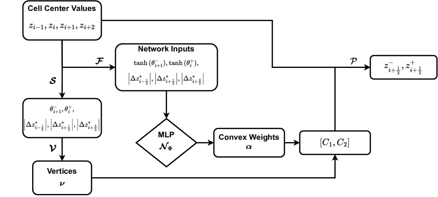
Figure 2: Schematic for the DSP-WENO reconstruction algorithm.

4.1 Data Selection

To generate training data for the neural network, we sample stencils consisting of four cells from parameterized smooth and discontinuous functions of the form listed in Table 2. The dataset has a 50/50 balanced split of smooth and discontinuous data. The section of the dataset consisting of smooth data consists of an equal representation of the three smooth types listed in Table 2. For discontinuous data, the jump will either be between the first and second cells, the second and third cells, or the third and fourth cells. In any case, using the four cell center values, we compute the jump ratios $\theta_{i+1}^{-}$ and $\theta_{i}^{+}$ and the absolute jumps across the three cell interfaces in the stencil, via ${\bm{\mathcal{S}}}$ defined in (30). Further, we compute a set of vertices using ${\bm{\mathcal{V}}}$ defined in (33). Finally, the true values at the cell interface $x_{i+\frac{1}{2}}$ are recorded to serve as target values that DSP-WENO will aim to reconstruct. Overall, the dataset consists of 100,000 samples, roughly corresponding to 50,000 discontinuous samples and 50,000 smooth samples.

No.	Type	$u(x)$	Parameters
1	Smooth	$ax^{3}+bx^{2}+cx+d$	$a,b,c,d\in\mathbb{U}[-10,10]$
2	Smooth	$(x-a)(x-b)(x-c)+d$	$a,b,c,d\in\mathbb{U}[-2,2]$
3	Smooth	$\sin{(a\pi x+b)}$	$a,b\in\mathbb{U}[-2,2]$
4	Discontinuous	$\begin{cases}ax+b\text{ if }x\leq 0.5\\ cx+d\text{ if }x>0.5\end{cases}$	$a,b,c,d\in\mathbb{U}[-5,5]$

Table 2: Functions used in constructing the training dataset where $\mathbb{U}[p,q]$ denotes the uniform distribution on the interval $[p,q].$

Remark 4.

We do not use solutions to conservation laws to train the network. We instead generate functions of varying regularity that canonically represent the local solution features we can expect to observe in solutions to conservation laws. Thus, there is an insignificant cost in generating the training data. A similar strategy was also considered in [45, 46].

Remark 5.

In our experiments, we noticed that the performance of DSP-WENO, particularly in the framework of TeCNO schemes, was highly dependent on the training set used to train DSP-WENO. In other words, the training set is itself a hyperparameter, that needs to be carefully constructed based on domain expertise.

4.2 Vertex Selection Algorithm

In this section, we describe the vertex selection algorithm that defines the map ${\bm{\mathcal{V}}}$ in (33). As discussed in Section 3.3 and listed in Table 1, there is a feasible region $\Omega_{C}$ associated with each $\Omega_{\Theta}$. Any choice of $(C_{1},C_{2})$ in the feasible region leads to consistent WENO weights which are guaranteed to satisfy the sign property and yield third-order accuracy in smooth regions. We show below that the $\Omega_{C}$ constructed to satisfy the various feasibility constraints leads to a convex polygon in $\mathbb{R}^{2}$. The objective with the neural network approach is to learn how to explore these $\Omega_{C}$ to better select $(C_{1},C_{2})$. In comparison, SP-WENO and SP-WENOc have handcrafted weight selection strategies that suffer from significant overshoots near discontinuities in the TeCNO framework. DSP-WENO aspires to mitigate this behavior through a data-driven search in the feasible regions.

Now, we discuss how the vertices of the convex $\Omega_{C}$ are selected. The fully-detailed algorithm can be found in Algorithm 1. Note that the vertex algorithm is applied for each four-cell stencil in the mesh. With the exception of cases 2 and 3 (see Table 1), the vertex selection for most scenarios is quite straight-forward. This is due to the fact that all cases besides 2 and 3 do not require an additional accuracy constraint, and so we only need to select vertices that yield a convex figure that satisfies the sign property and consistency of the WENO weights. Cases 2 and 3 are more involved since we do require that $C_{1},C_{2}=\mathcal{O}(h)$ in smooth regions. To address this, we construct an $\mathcal{O}(h)$ region in $\mathbb{R}^{2}$ as depicted in Figure 3. The dashed lines enclose a box representing the consistency requirements for the perturbations, i.e., $-3/8\leq C_{1},C_{2}\leq 1/8$. The $\mathcal{L}=1$ line shown in orange separates the regions satisfying the sign property for Cases 2 and 3, represented as solid dark and light grey regions respectively. Within these grey regions, we construct smaller sub-regions that also satisfy the accuracy constraints. These sub-regions are shown in blue and green, and form the required feasible regions $\Omega_{C}$ for cases 2 and 3. To construct these sub-regions, we first define the box $\mathcal{H}=[\gamma_{2},\gamma_{1}]\times[\gamma_{2},\gamma_{1}]\subset[-3/8,1/8]\times[-3/8,1/8]$ where

$$\gamma_{1} =\min{\left(\max{\left(|\Delta z_{i-\frac{1}{2}}^{*}|,|\Delta z_{i+\frac{1}{2}}^{*}|,|\Delta z_{i+\frac{3}{2}}^{*}|\right)},\frac{1}{8}\right)},$$ (38)

$$\gamma_{2} =-\min{\left(\max{\left(|\Delta z_{i-\frac{1}{2}}^{*}|,|\Delta z_{i+\frac{1}{2}}^{*}|,|\Delta z_{i+\frac{3}{2}}^{*}|\right)},\frac{3}{8}\right)}.$$

The region $\mathcal{H}$ is shown as a red dotted box in Figure 3. Note that when the $z$ on the local stencil is smooth, $|\Delta z_{i-\frac{1}{2}}^{*}|,|\Delta z_{i+\frac{1}{2}}^{*}|,|\Delta z_{i+\frac{3}{2}}^{*}|=\mathcal{O}(h)$. Thus, we ensure that $\gamma_{1},\gamma_{2}=\mathcal{O}(h)$, and searching for $(C_{1},C_{2})$ inside $\mathcal{H}$ would constrain $C_{1},C_{2}=\mathcal{O}(h)$, which is the order constraint for cases 2 and 3 assuming smoothness for $z$. When a discontinuity is present, $\mathcal{H}$ can potentially expand to the whole consistency region for $C_{1},C_{2}$. With the line $\mathcal{L}=1$ splitting $\mathcal{H}$, we have that the feasible region for Case 2 consists of the region above $\mathcal{L}=1$ and that of Case 3 consists of the region below $\mathcal{L}=1$. We further note that the closer the perturbations are to zero, the more accurate the reconstruction. In smooth regions, this is desirable, but near discontinuities, capturing shocks becomes the priority, so searching a wider search space becomes important.

As shown in Figure 3, the line $\mathcal{L}=1$ splits $\mathcal{H}$ into a triangular and pentagonal $\Omega_{C}$ region, with two out of three and two out of five vertices lying on the line $\mathcal{L}=1$, respectively. A peculiarity of choosing $(C_{1},C_{2})$ on this line is that it ensures the left and right reconstructed states at the interface are equal, i.e, $\llbracket z\rrbracket_{i+\frac{1}{2}}=0$. As discussed in Section 3.2, a zero reconstruction jump is undesirable in the vicinity of a discontinuity in the TeCNO framework. When choosing $(C_{1},C_{2})$ from a triangular region, two of whose vertices are on this line, which biases the selection to be on this line (this is what we also observed in practice). Thus, when constructing a triangular $\Omega_{C}$ above or below $\mathcal{L}=1$, we do not use the triangle that is a part of $\mathcal{H}$. Instead, we replace one of the vertices lying on $\mathcal{L}=1$ with another vertex pulled away from this line (without violating the consistency and sign property constraints) to form a flipped triangular $\Omega_{C}$ that is outside of $\mathcal{H}$. This flipped $\Omega_{C}$ still satisfies $C_{1},C_{2}=\mathcal{O}(h)$, and thus any point selected in this triangle will also satisfy this constraint. For instance, let us consider Case 2 when $\psi^{+}<-1$, where $\Omega_{C}$ is triangular (see Figure 3(c),(d)). In this scenario, according to Algorithm 1, the vertex outside $\mathcal{H}$ is $(\gamma_{2},\frac{1}{8}(1+\psi^{-})-\gamma_{1}\psi^{-})$. For smooth regions, $C_{1}=\gamma_{2}=\mathcal{O}(h)$. Further, we can deduce that $(1+\psi^{-})=\mathcal{O}(h)$. Since $\gamma_{1}=\mathcal{O}(h)$, it is clear that $C_{2}=\frac{1}{8}(1+\psi^{-})-\gamma_{1}\psi^{-}=\mathcal{O}(h)$. Similar arguments can be made for Case 3 when $-1<\psi^{+}<0$ where $\Omega_{C}$ is once again triangular (see Figure 3(a),(b)).

The number of vertices needed to construct a convex figure across all the possible scenarios is at most five. Thus, to ensure that the neural network always outputs the same number of convex weights $\bm{\alpha}$ corresponding to the vertices, we constrain the output dimension of the network to be five. In the various scenarios where the number of vertices is less than five, we augment the set of vertices to a set of five vertices by including either redundant vertices or some averaged state of the figure’s vertices. For instance, in Cases 2 and 3, when the feasible region is a triangle, we augment the set of three vertices with the centroid of the triangle twice.

Remark 6.

When constructing the triangular $\Omega_{C}$ for Cases 2 and 3, we do not discard all vertices lying on $\mathcal{L}=1$. This is because while $\llbracket z\rrbracket_{i+\frac{1}{2}}=0$ is not desirable near discontinuities, it does lead to better accuracy near smooth regions. Thus, we retain at least one of these vertices to maintain a balance in performance between smooth and discontinuous reconstructions.

Remark 7.

We do not modify the vertices of the pentagonal $\Omega_{C}$ obtained in Cases 2 and 3, as only two of the five vertices are on $\mathcal{L}=1$. Thus, the pentagonal regions do not suffer from the biasing issue faced by triangular $\Omega_{C}$.

Remark 8.

The vertex modification algorithm for the triangular $\Omega_{C}$ is not unique. After experimenting with a few configurations of choosing the shifted vertex, we found the one used in Algorithm 1 yields the best performance.

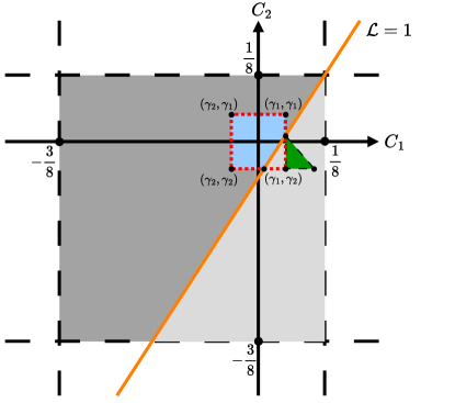
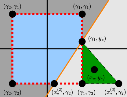
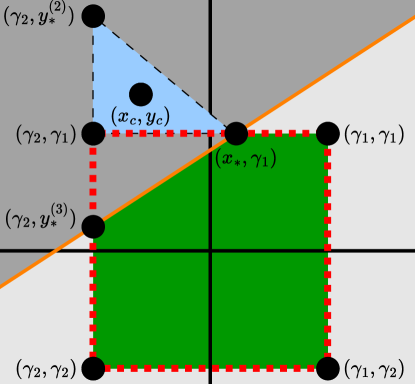
Figure 3: Feasible region for Case 2 (dark grey) and Case 3 (light grey). The $\mathcal{O}(h)$ box $\mathcal{H}$ (outlined by red dots) is centered about the origin. The vertex selection algorithm further restricts the search space to the blue and green regions for Case 2 and Case 3, respectively. (a) $\psi^{+}\in(-1,0)$ with a zoomed in view in (b), (c) $\psi^{+}\in(-\infty,-1)$ with a zoomed in view in (d).

Algorithm 1 Vertex Selection Algorithm

Input: Jump ratios $\theta_{i+1}^{-}$, $\theta_{i}^{+}$ and scaled absolute jumps $|\Delta z_{i-\frac{1}{2}}^{*}|$, $|\Delta z_{i+\frac{1}{2}}^{*}|$, $|\Delta z_{i+\frac{3}{2}}^{*}|$
Output: Set of vertices $\bm{\nu}=\left[\bm{\nu}_{1},\bm{\nu}_{2},\bm{\nu}_{3},\bm{\nu}_{4},\bm{\nu}_{5}\right]$

1:Evaluate $\psi^{\pm}$ according to (16), and $\gamma_{1},\gamma_{2}$ according to (38)

2:if $\theta_{i+1}^{-},\theta_{i}^{+}>1$ then

3:    $\bm{\nu}=\left[(\frac{1}{8},\frac{1}{8}),(\frac{1}{8},\frac{1}{8}),(\frac{1}{8},\frac{1}{8}),(\frac{1}{8},\frac{1}{8}),(\frac{1}{8},\frac{1}{8})\right]$

4:else if $\theta_{i+1}^{-}>1$, $\theta_{i}^{+}<1$ then

5:    if $\psi^{+}<-1$ then

6:         $x_{*}=\frac{1}{8}(1+\psi^{+})-\gamma_{1}\psi^{+}$

7:         if $x_{*}<\gamma_{2}$ then

8:             $\hat{x}=\frac{(\psi^{-})^{2}+\psi^{-}}{8((\psi^{-})^{2}+1)}$,    $\hat{y}=\frac{1}{8}(1+\psi^{-})-\hat{x}\psi^{-}$

9:             $\bm{\nu}=\left[(\hat{x},\hat{y}),(\hat{x},\hat{y}),(\hat{x},\hat{y}),(\hat{x},\hat{y}),(\hat{x},\hat{y})\right]$

10:         else

11:             $y_{*}^{(2)}=\frac{1}{8}(1+\psi^{-})-\gamma_{1}\psi^{-}$

12:             $x_{c}=\frac{1}{3}(2\gamma_{2}+x_{*})$,    $y_{c}=\frac{1}{3}(2\gamma_{1}+y_{*}^{(2)})$

13:             $\bm{\nu}=\left[(\gamma_{2},\gamma_{1}),(x_{*},\gamma_{1}),(\gamma_{2},y_{*}^{(2)}),(x_{c},y_{c}),(x_{c},y_{c})\right]$

14:         end if

15:    else

16:         $y_{*}=\frac{1}{8}(1+\psi^{-})-\gamma_{1}\psi^{-}$

17:         if $y_{*}<\gamma_{2}$ then

18:             $\bm{\nu}=\left[(\gamma_{2},\gamma_{1}),(\gamma_{1},\gamma_{1}),(\gamma_{2},\gamma_{2}),(\gamma_{1},\gamma_{2}),(0,0)\right]$

19:         else

20:             $x_{*}^{(2)}=\frac{1}{8}(1+\psi^{+})-\gamma_{2}\psi^{+}$

21:             $\bm{\nu}=\left[(\gamma_{2},\gamma_{1}),(\gamma_{1},\gamma_{1}),(\gamma_{2},\gamma_{2}),(\gamma_{1},y_{*}),(x_{*}^{(2)},\gamma_{2})\right]$

22:         end if

23:    end if

24:else if $\theta_{i+1}^{-}<1$, $\theta_{i}^{+}>1$ then

25:    if $\psi^{+}<-1$ then

26:         $x_{*}=\frac{1}{8}(1+\psi^{+})-\gamma_{1}\psi^{+}$

27:         if $x_{*}<\gamma_{2}$ then

28:             $\bm{\nu}=\left[(\gamma_{2},\gamma_{1}),(\gamma_{1},\gamma_{1}),(\gamma_{2},\gamma_{2}),(\gamma_{1},\gamma_{2}),(0,0)\right]$

29:         else

30:             $y_{*}^{(3)}=\frac{1}{8}(1+\psi^{-})-\gamma_{2}\psi^{-}$

31:             $\bm{\nu}=\left[(\gamma_{1},\gamma_{2}),(\gamma_{1},\gamma_{1}),(\gamma_{2},\gamma_{2}),(x_{*},\gamma_{1}),(\gamma_{2},y_{*}^{(3)})\right]$

32:         end if

33:    else

34:         $y_{*}=\frac{1}{8}(1+\psi^{-})-\gamma_{1}\psi^{-}$

35:         if $y_{*}<\gamma_{2}$ then

36:             $\hat{x}=\frac{(\psi^{-})^{2}+\psi^{-}}{8((\psi^{-})^{2}+1)}$,    $\hat{y}=\frac{1}{8}(1+\psi^{-})-\hat{x}\psi^{-}$

37:             $\bm{\nu}=\left[(\hat{x},\hat{y}),(\hat{x},\hat{y}),(\hat{x},\hat{y}),(\hat{x},\hat{y}),(\hat{x},\hat{y})\right]$

38:         else

39:             $x_{*}^{(3)}=\frac{1}{8}(1+\psi^{+})-\gamma_{1}\psi^{+}$

40:             $x_{c}=\frac{1}{3}(2\gamma_{1}+x_{*}^{(3)})$,    $y_{c}=\frac{1}{3}(2\gamma_{2}+y_{*})$

41:             $\bm{\nu}=\left[(\gamma_{1},\gamma_{2}),(x_{*}^{(3)},\gamma_{2}),(\gamma_{1},y_{*}),(x_{c},y_{c}),(x_{c},y_{c})\right]$

42:         end if

43:    end if

44:else if $\theta_{i+1}^{-}==1$, $\theta_{i}^{+}>1$ then

45:    $\bm{\nu}=\left[(\frac{1}{8},-\frac{3}{8}),(\frac{1}{8},\frac{1}{8}),(\frac{1}{8},\frac{1}{8}),(\frac{1}{8},-\frac{3}{8}),(\frac{1}{8},-\frac{1}{8})\right]$

46:else if $\theta_{i}^{+}==1$, $\theta_{i+1}^{-}>1$ then

47:    $\bm{\nu}=\left[(\frac{1}{8},\frac{1}{8}),(\frac{1}{8},\frac{1}{8}),(-\frac{3}{8},\frac{1}{8}),(-\frac{3}{8},\frac{1}{8}),(-\frac{1}{8},\frac{1}{8})\right]$

48:else

49:    $\bm{\nu}=\left[(\frac{1}{8},\frac{1}{8}),(\frac{1}{8},-\frac{3}{8}),(-\frac{3}{8},-\frac{3}{8}),(-\frac{3}{8},\frac{1}{8}),(-\frac{1}{8},-\frac{1}{8})\right]$

50:end if

4.3 Neural Network Architecture

Since the neural network only has to learn to generate five convex weights given a relatively small feature space as input, we use a fairly simple network architecture. In particular, we employ an MLP that consists of three hidden layers with five neurons each, and an output layer also containing five neurons, leading to an MLP with $\#{\bm{\Phi}}=120$ trainable parameters. The ReLU activation function is used in the hidden layers. Following the output layer, we use the softmax activation function to ensure that the network predicts a vector of convex vertex weights $\bm{\alpha}$. The predicted $\bm{\alpha}$ are used to obtain the perturbation according to (34), which are then used to estimate the cell interface reconstructions according to (35).

Other variations of the the MLP’s architecture (including activation functions) were considered, but ultimately this architecture yielded the best results.

4.4 Training Setup

We use the $l_{1}$ loss function (36) to calculate the difference between the actual values at the cell interface and the reconstructed values that are obtained from DSP-WENO. The objective of the training process is to minimize this loss. To train the neural network, we use the Adam optimizer [25] with optimizer parameters $\beta_{1}=0.5$, $\beta_{2}=0.9$, and a weight decay regularization of $10^{-5}$. We use a learning rate of 0.001. We perform a training/validation/test split in a 0.6/0.2/0.2 proportion, so that we can assess the performance on withheld data (the validation set) and then test on unseen data (the test set) when the network is finished being trained. We use mini-batches of size 500 and reshuffle the training set every epoch. The network is trained using PyTorch for 50 epochs on a 2.60 GHz Intel Core i7-10750H CPU. The training time for training one instance of this MLP is less than 30 seconds. We perform five training runs with different random initializations of the network weight and biases and select the network that performs the best on the test set.

4.5 Properties of DSP-WENO

DSP-WENO by construction satisfies all properties of SP-WENO with the exception of the mirror property. This property is lost due to the nature of the vertex selection algorithm and computation of the convex weights by the neural network. While it is possible to have pursued a construction that preserves the mirror property, we choose to omit it so as not to overly constrain the network. Additionally, DSP-WENO satisfies the following stability estimate for the reconstructed jump in terms of the original jumps.

Lemma 3.

(Bounds on jumps) The DSP-WENO reconstructed jump satisfies the following estimate:

$$\left|\llbracket z\rrbracket_{i+\frac{1}{2}}\right|\leq\frac{1}{2}\left|\Delta z_{i-\frac{1}{2}}\right|+\left|\Delta z_{i+\frac{1}{2}}\right|+\frac{1}{2}\left|\Delta z_{i+\frac{3}{2}}\right|\hskip 8.53581pt\forall\hskip 2.84526pti\in\mathbb{Z}.$$ (39)

Proof.

If $\Delta z_{i+\frac{1}{2}}=0$, the bound will clearly be satisfied since $|\llbracket z\rrbracket_{i+\frac{1}{2}}|=0$ in this case by construction of DSP-WENO. Hence, we assume $\Delta z_{i+\frac{1}{2}}\neq 0$. We start with the explicit expression for $\llbracket z\rrbracket_{i+\frac{1}{2}}$ (17) and expand

$$\llbracket z\rrbracket_{i+\frac{1}{2}} =\frac{1}{2}\left[\tilde{w}_{0}\left(1-\theta_{i+1}^{-}\right)+w_{1}\left(1-\theta_{i}^{+}\right)\right]\Delta z_{i+\frac{1}{2}}$$

$$=\frac{1}{2}\left[\left(\frac{1}{4}-2C_{2}\right)\left(1-\frac{\Delta z_{i+\frac{3}{2}}}{\Delta z_{i+\frac{1}{2}}}\right)+\left(\frac{1}{4}-2C_{1}\right)\left(1-\frac{\Delta z_{i-\frac{1}{2}}}{\Delta z_{i+\frac{1}{2}}}\right)\right]\Delta z_{i+\frac{1}{2}}$$

$$=\left(C_{1}-\frac{1}{8}\right)\Delta z_{i-\frac{1}{2}}+\left(\frac{1}{4}-C_{1}-C_{2}\right)\Delta z_{i+\frac{1}{2}}+\left(C_{2}-\frac{1}{8}\right)\Delta z_{i+\frac{3}{2}}.$$

By consistency, we have $-3/8\leq C_{1},C_{2}\leq 1/8$. Thus, the absolute value of the jump is clearly bounded

$$\left|\llbracket z\rrbracket_{i+\frac{1}{2}}\right| \leq\left|C_{1}-\frac{1}{8}\right|\left|\Delta z_{i-\frac{1}{2}}\right|+\left|\frac{1}{4}-C_{1}-C_{2}\right|\left|\Delta z_{i+\frac{1}{2}}\right|+\left|C_{2}-\frac{1}{8}\right|\left|\Delta z_{i+\frac{3}{2}}\right|$$

$$\leq\frac{1}{2}\left|\Delta z_{i-\frac{1}{2}}\right|+\left|\Delta z_{i+\frac{1}{2}}\right|+\frac{1}{2}\left|\Delta z_{i+\frac{3}{2}}\right|.$$

∎

Remark 9.

The estimate (39) is not unique to DSP-WENO and is a consequence of the sign property constraint (18). Thus, it is also satisfied by every variant of SP-WENO. However, it was shown in [16] that the original SP-WENO satisfies a sharper bound which is attributed to the fact the the reconstructed jump is zero is many cases.

5 Numerical Results

In this section, we present several numerical results to demonstrate the efficacy of the proposed DSP-WENO approach. We consider both 1D and 2D test cases for the evolution of scalar and systems of conservation laws. In 1D, we discretize a domain $[a,b]$ using an $N$-cell uniform mesh with $h=\frac{b-a}{N}$

$$x_{i+\frac{1}{2}}:=a+ih,\hskip 8.53581ptx_{i}=\frac{x_{i-\frac{1}{2}}+x_{i+\frac{1}{2}}}{2},\hskip 8.53581pti=0,...,N.$$

In 2D, we discretize the domain $[a,b]\times[c,d]$ using a uniform mesh (in each dimension) with $h_{x}=\frac{b-a}{N_{x}}$ and $h_{y}=\frac{d-c}{N_{y}}$. The mesh is constructed as

$$x_{i+\frac{1}{2}}:=a+ih_{x},\hskip 8.53581ptx_{i}=\frac{x_{i-\frac{1}{2}}+x_{i+\frac{1}{2}}}{2},\hskip 8.53581pti=0,...,N_{x},$$

$$y_{j+\frac{1}{2}}:=c+jh_{y},\hskip 8.53581pty_{j}=\frac{y_{j-\frac{1}{2}}+y_{j+\frac{1}{2}}}{2},\hskip 8.53581ptj=0,...,N_{y}.$$

Ghost cells are introduced to extend the mesh as needed while imposing either periodic or Neumann boundary conditions. In all evolution cases, we use the TeCNO4 numerical flux, consisting of the fourth-order accurate entropy conservative flux (7) and various sign-preserving reconstruction methods for the diffusion operator. The CFL may vary across problems and is specified in each case. SSP-RK3 (see [18]) is used for time-marching in all evolution test cases.

5.1 Reconstruction Accuracy

Before proceeding to solve conservation laws, we demonstrate the reconstruction accuracy of DSP-WENO. We consider the reconstruction of a smooth inclined sine wave

$$u(x)=\sin{(10\pi x)}+x,\hskip 8.53581ptx\in[0,1],$$

as the mesh size $h$ is varied. To compute the error in the interface values, we evaluate

$$\|u^{-}_{i+\frac{1}{2}}-u(x_{i+\frac{1}{2}})\|_{L^{1}_{h}}+\|u^{+}_{i+\frac{1}{2}}-u(x_{i+\frac{1}{2}})\|_{L^{1}_{h}},$$

where the discrete $L^{1}$ norm is defined as

$$\|(\cdot)_{i}\|_{L^{1}_{h}}=\sum_{i=1}^{N}|(\cdot)_{i}|h.$$

Table 3 shows the errors and corresponding convergence rates for ENO3, SP-WENO, SP-WENOc, and DSP-WENO. All reconstruction methods achieve the expected third-order convergence with the SP-WENO variants exhibiting super-convergence. Note that the errors of DSP-WENO are about an order of magnitude larger than those of SP-WENO and SP-WENOc while being similar to ENO3 on the finer meshes.

Now, we consider a continuous function with a sharp connection between two linear components to mimic a discontinuity:

$$u(x)=\begin{cases}\frac{1}{2}x&\text{ if }-0.5\leq x<0\\ \frac{x}{\epsilon}&\text{ if }0\leq x\leq\epsilon\\ x-\epsilon+1&\text{ if }\epsilon<x\leq 0.5\end{cases},$$

where $\epsilon$ is chosen as 0.001. We reconstruct on a mesh consisting of 1000 cells, ensuring that a single cell is sitting inside the jump. In other words, we are simulating a scenario where the discontinuity is not perfectly resolved. Figure 4 shows the left and right reconstructed interface values for ENO3, SP-WENO, SP-WENOc, and DSP-WENO, zoomed into the region close to the simulated discontinuity. Figure 4 also features bar plots that show the actual jump in cell center values and the reconstructed jump at the interface for each method. The left and right reconstructed values are almost identical outside of the $0\leq x\leq\epsilon$ region for all the methods, and thus not visible in the figure given the scale of the jump. However, inside the pseudo-shock where a cell (let us call it $I_{0}$) lies, SP-WENO and SP-WENOc do not fully capture the non-zero jumps. At the left interface of $I_{0}$, SP-WENO results in a very small reconstructed jump, while SP-WENOc leads to a larger jump but which is still an order of magnitude smaller as compared to the jump at the right interface of $I_{0}$. On the other hand, ENO3 and DSP-WENO give rise to larger reconstructed jumps at both interfaces of $I_{0}$, which is the desirable behavior in the vicinity of discontinuities. In the numerical results that follow, we will see a visible impact of the reconstructed jump magnitude.

N	ENO3		SP-WENO		SP-WENOc		DSP-WENO
	$L_{h}^{1}$		$L_{h}^{1}$		$L_{h}^{1}$		$L_{h}^{1}$
	Error	Rate	Error	Rate	Error	Rate	Error	Rate
40	3.47e-2	-	7.27e-2	-	7.41e-2	-	1.65e-1	-
80	4.54e-3	2.93	5.85e-3	3.64	6.37e-3	3.54	3.01e-2	2.45
160	5.84e-4	2.96	4.45e-4	3.72	4.71e-4	3.76	2.83e-3	3.41
320	7.42e-5	2.98	3.29e-5	3.76	3.43e-5	3.78	2.14e-4	3.73
640	9.38e-6	2.98	2.37e-6	3.79	2.46e-6	3.80	1.55e-5	3.78
1280	1.17e-6	3.00	1.68e-7	3.82	1.74e-7	3.82	1.22e-6	3.67
2560	1.47e-7	3.00	1.18e-8	3.84	1.21e-8	3.84	1.13e-7	3.44

Table 3: Reconstruction accuracy for inclined sine wave.

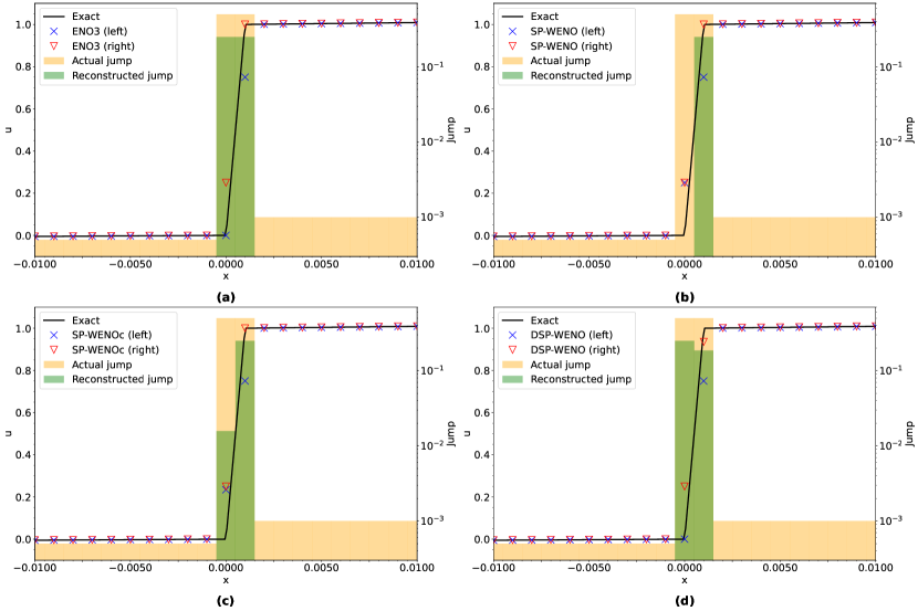
Figure 4: Reconstruction of a simulated discontinuity, which is not well-resolved, using: (a) ENO3, (b) SP-WENO, (c) SP-WENOc, (d) DSP-WENO.

5.2 Linear Advection

Consider the one-dimensional scalar linear advection equation

$$u_{t}+cu_{x}=0.$$

For the 1D scalar case, the finite difference TeCNO4 numerical flux (13) simplifies to

$$f_{i+\frac{1}{2}}=\tilde{f}^{2p}_{i+\frac{1}{2}}-a_{i+\frac{1}{2}}\left(v_{i+\frac{1}{2}}^{+}-v_{i+\frac{1}{2}}^{-}\right),$$ (40)

where $v:=\eta^{\prime}(u)=u$ is the entropy variable corresponding to the square entropy $\eta(u)=\frac{u^{2}}{2}$. The entropy conservative component $\tilde{f}^{2p}$ of the flux is constructed using (7) with the following second-order entropy conservative flux

$$\tilde{f}_{i+\frac{1}{2}}=c\frac{(u_{i}+u_{i+1})}{2}.$$

Additionally, $a_{i+\frac{1}{2}}=|c|$ for the linear advection model. We set the convective velocity $c=1$ for all test cases.

5.2.1 Smooth Initial Condition

We consider two test cases with smooth initial conditions on $[-\pi,\pi]$ with periodic boundary conditions.

Test 1: $u_{0}(x)=\sin(x)$, simulated until final time $T=0.5$ with CFL = 0.4.

Test 2: $u_{0}(x)=\sin^{4}(x)$, simulated until final time $T=0.5$ with CFL = 0.5.

Table 4 shows the $L_{h}^{1}$ errors with various reconstructions for both of these test cases. ENO3 works well for Test 1 and achieves third-order convergence with marginally smaller absolute errors when compared to the results of SP-WENO, SP-WENOc, and DSP-WENO. However, the convergence rate with ENO3 deteriorates in Test 2. It has been observed in [48] that ENO3 performs poorly for this test case with the MUSCL scheme due to linear instabilities, and we observe the same issues with ENO3 in the TeCNO framework (also seen in [16]). The other reconstruction methods are stable, as SP-WENO, SP-WENOc, and DSP-WENO do not suffer from this issue. All three reconstruction methods achieve third-order convergence, though the errors of DSP-WENO are about an order of magnitude larger than those of SP-WENO and SP-WENOc. Moreover, SP-WENO and SP-WENOc exhibit super-convergence. This can be attributed to the reconstructed jump often being zero, which effectively disables the local diffusion and results in the local numerical flux entirely consisting of the fourth-order entropy conservative flux.

DSP-WENO is much more dissipative, so in these test cases and in general for smooth regions, we observe larger errors (though the third-order convergence is still maintained). However, this increase in diffusion leads to improved performance over SP-WENO and SP-WENOc when the solution is not smooth (see the results of Sections 5.2.2, 5.3, and 5.4).

	N	ENO3		SP-WENO		SP-WENOc		DSP-WENO
		$L_{h}^{1}$		$L_{h}^{1}$		$L_{h}^{1}$		$L_{h}^{1}$
		Error	Rate	Error	Rate	Error	Rate	Error	Rate
	100	3.23e-5	-	6.90e-5	-	6.80e-5	-	1.66e-4	-
	200	4.04e-6	3.00	7.65e-6	3.17	7.48e-6	3.18	3.58e-5	2.21
Test 1	400	5.05e-7	3.00	8.29e-7	3.20	8.17e-7	3.20	4.57e-6	2.97
	600	1.50e-7	3.00	2.26e-7	3.20	2.23e-7	3.20	1.35e-6	3.02
	800	6.31e-8	3.00	8.72e-8	3.31	8.60e-8	3.31	5.72e-7	2.97
	1000	3.23e-8	3.00	4.21e-8	3.27	4.15e-8	3.26	2.95e-7	2.97
	100	1.48e-3	-	1.52e-3	-	1.46e-3	-	1.87e-3	-
	200	1.98e-4	2.91	1.68e-4	3.18	1.68e-4	3.12	2.61e-3	2.84
Test 2	400	2.58e-5	2.94	1.79e-5	3.23	1.78e-5	3.23	3.35e-5	2.96
	600	8.25e-6	2.81	4.69e-6	3.31	4.70e-6	3.29	9.59e-6	3.08
	800	4.64e-6	2.00	1.81e-6	3.31	1.80e-6	3.33	3.93e-6	3.10
	1000	3.46e-6	1.31	8.64e-7	3.32	8.61e-7	3.31	2.03e-6	2.96

Table 4: Linear advection Tests 1 and 2 with TeCNO4 flux.

5.2.2 Discontinuous Initial Condition

Test 3 The domain is $[0,1.4]$, final time is $T=1.4$, and CFL = 0.2, with initial profile

$$u_{0}(x)=\begin{cases}10(x-0.2)&\text{if }0.2<x\leq 0.3\\ 10(0.4-x)&\text{if }0.3<x\leq 0.4\\ 1&\text{if }0.6<x\leq 0.8\\ 100(x-1)(1.2-x)&\text{if }1.0<x\leq 1.2\\ 0&\text{otherwise}\end{cases},$$

and periodic boundary conditions. Note that the initial profile is a composition of shapes with different orders of regularity. The results on a mesh with 100 cells for various reconstruction methods are shown in Figure 5. ENO2 leads to the most dissipative approximation on this mesh. Overall, ENO3 yields the best performance, as its solution is the closest to the exact solution while avoiding any spurious oscillatory behavior. The solution obtained with DSP-WENO appears to be marginally more dissipative than ENO3, but without exhibiting the large undershoots/overshoots observed when using SP-WENO or SP-WENOc.

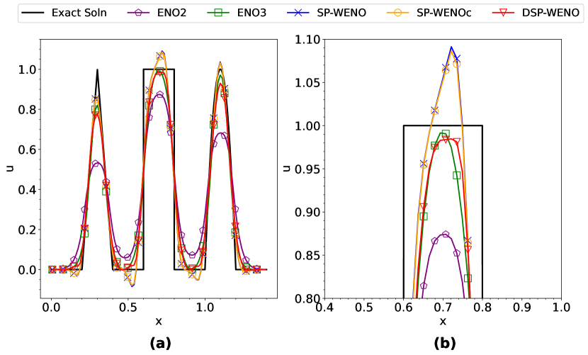
Figure 5: Linear advection Test 3: Solution with TeCNO4 at time $T=1.4$. (a) Comparison of different reconstruction methods for $x\in[0,1.4]$, (b) Zoomed in comparison for $x\in[0.4,1]$.

5.3 Burgers’ Equation

We now consider the Burgers’ Equation

$$u_{t}+\left(\frac{u^{2}}{2}\right)_{x}=0.$$

As with linear advection, we use (40) with entropy variables $v=u$ corresponding to the square entropy $\eta(u)=\frac{u^{2}}{2}$. The high-order entropy conservative flux (7) makes use of the following second-order entropy conservative flux

$$\tilde{f}_{i+\frac{1}{2}}=\frac{(u_{i}^{2}+u_{i+1}^{2}+u_{i}u_{i+1})}{6}.$$

Additionally, we take $a_{i+\frac{1}{2}}=\frac{|u_{i}|+|u_{i+1}|}{2}$.

Test 1: The domain is $[-1,1]$, final time is $T=0.5$, and CFL = 0.4, with initial profile

$$u_{0}(x)=\begin{cases}3&\text{if }x<0\\ -1&\text{if }x>0\end{cases},$$

and Neumann boundary conditions. The mesh consists of 100 cells. Figure 6 shows that all the solutions experience oscillations. This is a fundamental problem with high-order TeCNO schemes, so there often is no way to completely eliminate the overshooting behavior without introducing additional diffusion. However, we observe that DSP-WENO performs better in mitigating the oscillations leading up to the overshoot.

Remark 10.

While omitted from Figure 6, we found that these oscillations cannot be avoided even with the most restrictive linear reconstruction using the minmod limiter, which also satisfies the sign property [14].

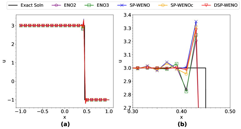
Figure 6: Burgers’ Test 1: Solution with TeCNO4 at time $T=0.5$. (a) Comparison of different reconstruction methods for $x\in[-1,1]$, (b) Zoomed in comparison for $x\in[0.3,0.5]$.

Test 2: The domain is $[-4,4]$, final time is $T=0.4$, and CFL = 0.4, with initial profile

$$u_{0}(x)=\begin{cases}3&\text{if }-1\leq x<-0.5\\ 1&\text{if }-0.5\leq x<0\\ 3&\text{if }0\leq x<0.5\\ 2&\text{if }0.5\leq x<1\\ \sin{(\pi x)}&\text{if }|x|>1\end{cases},$$

and periodic boundary conditions. This initial condition is taken from [45] and contains both smooth and discontinuous features. When solved on a mesh with 400 cells, Figure 7 shows that SP-WENO and SP-WENOc perform poorly near the shocks, especially at $x=1.3$ where the overshoots are relatively large. While the oscillations are still present with DSP-WENO, they are significantly mitigated when compared to the other SP-WENO methods.

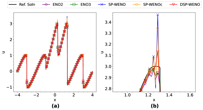
Figure 7: Burgers’ Test 2: Solution with TeCNO4 at time $T=0.4$. Comparison of different reconstruction methods for various domains: (a) $x\in[-4,4]$, (b) $x\in[0.86,1.65]$.

5.4 Euler Equations

We now consider the Euler equations described by

$$\frac{\partial}{\partial t}\begin{pmatrix}\rho\\ \rho\textbf{u}\\ E\end{pmatrix}+\nabla\cdot\begin{pmatrix}\rho\textbf{u}\\ p\mathbf{I}+\rho(\textbf{u}\otimes\textbf{u})\\ (E+p)\textbf{u}\end{pmatrix}=\mathbf{0},$$

where $\rho$, $\textbf{u}=(\text{u}_{1},\text{u}_{2},\text{u}_{3})^{\top}$, and $p$ represent the fluid density, velocity, and pressure, respectively. Note that u is distinct from ${\bm{u}}$, with the latter representing the vector of conserved variables. $E$ is the total energy per unit volume given by

$$E=\rho\left(\frac{|\textbf{u}|^{2}}{2}+e\right).$$

where $e$ is the specific internal energy given by a caloric equation of state, $e=e(\rho,p)$. Here, we take the equation of state to be

$$e=\frac{p}{(\gamma-1)\rho},$$

where $\gamma=c_{p}/c_{v}$ denotes the ratio of specific heats. In all the test cases, we set $\gamma=1.4$.

For the Euler equations, a popular choice for the entropy-entropy flux pair [20] is

$$\eta=-\frac{\rho s}{\gamma-1},\hskip 8.53581pt\bm{q}=[q_{1},q_{2},q_{3}]=-\frac{\rho\textbf{u}^{\top}s}{\gamma-1},$$ (41)

where $s=\ln{(p)}-\gamma\ln{(\rho)}$ is associated with the thermodynamic specific entropy. The corresponding vector of entropy variables is given by

$${\bm{v}}=\begin{pmatrix}\frac{\gamma-s}{\gamma-1}-\beta|\textbf{u}|^{2},\hskip 8.53581pt2\beta\textbf{u}^{\top},\hskip 8.53581pt-2\beta\end{pmatrix}^{\top}.$$ (42)

where $\beta=\rho/(2p)$.

In the TeCNO scheme, we use the second-order kinetic energy preserving and entropy conservative (KEPEC) flux [5] and (7) to construct the fourth-order entropy conservative flux. In 1D, the KEPEC flux is given as:

$${\bm{f}}=\begin{pmatrix}F^{\rho}\\ F^{m}\\ F^{e}\end{pmatrix}=\begin{pmatrix}\hat{\rho}\overline{\text{u}}\\ \tilde{p}+\overline{\text{u}}F^{\rho}\\ F^{e}\end{pmatrix},\hskip 8.53581ptF^{e}=\left[\frac{1}{2(\gamma-1)\hat{\beta}}-\frac{1}{2}\overline{|\text{u}|^{2}}\right]F^{\rho}+\overline{\text{u}}F^{m},$$ (43)

where $\tilde{p}=\overline{\rho}/(2\overline{\beta})$ and $\beta=\rho/(2p)$. $\hat{\rho}$, $\hat{\beta}$ represent the logarithmic averages (see [22, 5]) of the respective positive quantities.

For the diffusion term in 1D, we use the Roe-type diffusion operator

$$\mathbf{D}_{i+\frac{1}{2}}=\tilde{\mathbf{R}}_{i+\frac{1}{2}}\mathbf{\Lambda}_{i+\frac{1}{2}}\tilde{\mathbf{R}}_{i+\frac{1}{2}}^{\top},$$ (44)

where $\mathbf{R}_{i+\frac{1}{2}}$ consists of the eigenvectors of the flux Jacobian $\partial_{{\bm{u}}}{\bm{f}}$ and

$$\mathbf{\Lambda}_{i+\frac{1}{2}}=\operatorname{diag}{\left(|u-a|,|u|,|u+a|\right)}_{i+\frac{1}{2}}.$$ (45)

In (45), $a=\sqrt{\gamma p/\rho}$ is the speed of sound in air. The matrices $\mathbf{D}_{i+\frac{1}{2}}$ and $\mathbf{\Lambda}_{i+\frac{1}{2}}$ are evaluated at some averaged state. For additional details on the diffusion operator, and the flux formulation in higher dimensions, we refer the readers to [5, 44].

5.4.1 1D Euler Equations

We begin our study of the Euler equations in one dimension.

Modified Sod Shock Tube: This is a shock tube problem [54] solved on the domain is $[0,1]$ with initial profile

$$(\rho,\text{u},p)=\begin{cases}(1,0.75,1)&\text{if }x<0.3\\ (0.125,0,0.1)&\text{if }x\geq 0.3\end{cases}.$$

It is solved on a domain with 400 cells with Neumann boundary conditions, up to a final time of $T=0.2$ with CFL=0.4. Figure 8 shows that SP-WENO and SP-WENOc exhibit significant overshoots, especially near the shock at $x\approx 0.72$. DSP-WENO markedly improves on the performance of both methods by featuring only very minor overshoots in comparison. Further, the accuracy in shock-capturing is comparable to ENO3, with a sharper resolution of the contact discontinuity at $x\approx 0.57$.

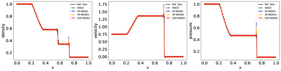
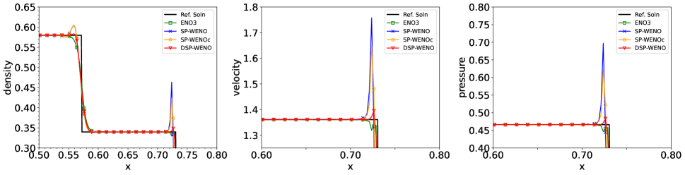
Figure 8: Modified Sod Shock Tube Test: Solution with TeCNO4 at time $T=0.2$ for $\rho$, u, and $p$. Comparison of different reconstruction methods for various domains: (a) $x\in[0,1]$ for $\rho$, u, and $p$, (b) $\rho$: $x\in[0.5,0.8]$, u: $x\in[0.6,0.8]$, $p$: $x\in[0.6,0.8]$.

Shu-Osher Test: This test case, proposed in [50], contains the interaction of an oscillatory smooth wave and a right-moving shock. The domain is $[-5,5]$, final time is $T=1.8$, and CFL = 0.4, with initial profile

$$(\rho,\text{u},p)=\begin{cases}(3.857143,2.629369,10.33333)&\text{if }x<-4\\ (1+0.2\sin{(5x)},0,1)&\text{if }x\geq-4\end{cases},$$

and Neumann boundary conditions. The mesh consists of 400 cells. This was one of the test cases presented in [44] where SP-WENOc significantly mitigates the overshoots near the shock as compared to SP-WENO, which is also what we observe in Figure 9. DSP-WENO is clearly the most dissipative of the methods (although comparable to ENO3) when focusing in the regions with smooth physical high-frequency oscillations. However, there is essentially no overshoot near the shock with DSP-WENO, which is a large improvement over SP-WENO and SP-WENOc.

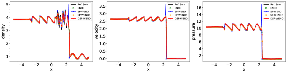
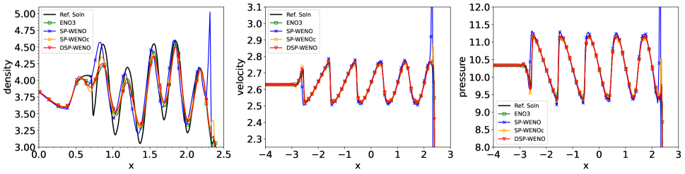
Figure 9: Shu-Osher Test: Solution with TeCNO4 at time $T=1.8$ for $\rho$, u, and $p$. Comparison of different reconstruction methods for various domains: (a) $x\in[-5,5]$ for $\rho$, u, and $p$, (b) $\rho$: $x\in[0,2.5]$, u: $x\in[-4,3]$, $p$: $x\in[-4,3]$.

Lax Test: For the Lax shock tube problem [29], the domain is $[-5,5]$, final time is $T=1.3$, and CFL = 0.4, with initial profile

$$(\rho,\text{u},p)=\begin{cases}(0.445,0.698,3.528)&\text{if }x<0\\ (0.5,0,0.571)&\text{if }x\geq 0\end{cases},$$

and Neumann boundary conditions. The mesh consists of 200 cells. Figure 10 shows that SP-WENO and SP-WENOc exhibit significant overshoots near the shocks. The solution obtained with DSP-WENO greatly minimizes the oscillatory behavior, similar to the previous test cases.

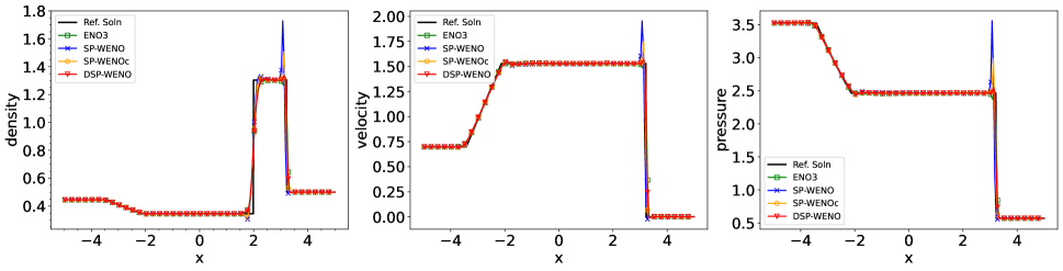
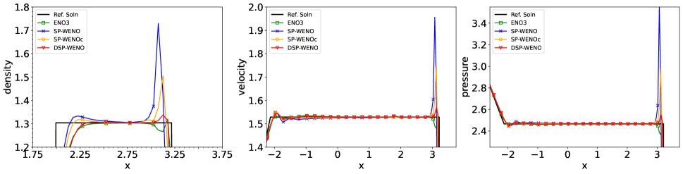
Figure 10: Lax Shock Tube Test: Solution with TeCNO4 at time $T=1.3$ for $\rho$, u, and $p$. Comparison of different reconstruction methods for various domains: (a) $x\in[-5,5]$ for $\rho$, u, and $p$, (b) $\rho$: $x\in[1.75,3.75]$, u: $x\in[-2.25,3.75]$, $p$: $x\in[-2.6,3.75]$.

Double Rarefaction: For this problem consisting of two rarefaction waves [34], the domain is $[-1,1]$, final time is $T=0.6$, and CFL = 0.4, with initial profile

$$(\rho,\text{u},p)=\begin{cases}(7,-1,0.2)&\text{if }x<0\\ (7,1,0.2)&\text{if }x\geq 0\end{cases},$$

and Neumann boundary conditions. This can be a challenging test case as the solution is close to vacuum near $x=0$. We solve the problem on a mesh consisting of 128 cells. With the absence of a discontinuity (except in the initial condition), the solutions obtained using ENO3, SP-WENOc, and DSP-WENO are very similar, as shown in Figure 11. Note that SP-WENO is omitted because the solver blows up due to the initial condition, even with lowering the CFL.

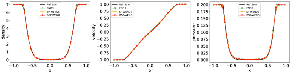
Figure 11: Double Rarefaction Test: Solution with TeCNO4 at time $T=0.6$ for $\rho$, u, and $p$. Comparison of different reconstruction methods for $x\in[-1,1]$ for $\rho$, u, and $p$.

5.4.2 2D Euler Equations

We continue our study of the Euler equations by considering several test cases in two dimensions.

Isentropic Vortex: In this problem, we consider the advection of a smooth isentropic vortex. This results in an entirely smooth solution, so we perform a mesh-refinement study here. The domain is $[-5,5]\times[-5,5]$, final time is $T=10$, and CFL = 0.5. The initial conditions are

$$\text{u}_{1}=1-\frac{\Gamma}{2\pi}y\exp{\left(\frac{1-r^{2}}{2}\right)},\hskip 8.53581pt\text{u}_{2}=\frac{\Gamma}{2\pi}x\exp{\left(\frac{1-r^{2}}{2}\right)},\hskip 8.53581pt\mathcal{T}=1-\frac{(\gamma-1)\Gamma^{2}}{8\gamma\pi^{2}}\exp{(1-r^{2})},$$

where $\mathcal{T}$ is the fluid temperature field, $r^{2}=x^{2}+y^{2}$ and $\Gamma=5$ (the vortex strength). Further, we have $\rho=\mathcal{T}^{1/(\gamma-1)}$ and $p=\mathcal{T}^{\gamma/(\gamma-1)}$ due to the isentropic conditions. Assuming periodic boundary condition, the vortex moves horizontal with unit velocity and completes one full periodic cycle at the final time. Table 5 shows $L_{h}^{1}$ errors with various reconstructions. We observe that ENO3 is unable to achieve third-order convergence, which we hypothesis is due to the linear instabilities with ENO [48]. The SP-WENO variants lead to third-order accuracy, with the results using DSP-WENO being more dissipative as compared to SP-WENO and SP-WENOc. We reiterate that this behavior is due to SP-WENO and SP-WENOc having zero reconstructed jumps in larger regions of the domain.

	N	ENO3		SP-WENO		SP-WENOc		DSP-WENO
		Error	Rate	Error	Rate	Error	Rate	Error	Rate
	50	1.17e-1	-	7.56e-2	-	7.51e-2	-	1.64e-1	-
	100	1.75e-2	2.74	6.62e-3	3.51	6.73e-3	3.48	1.91e-2	3.10
Density	150	7.13e-3	2.22	1.37e-3	3.88	1.40e-3	3.87	5.25e-3	3.19
	200	3.60e-3	2.38	4.59e-4	3.80	4.69e-4	3.80	2.14e-3	3.12
	300	1.48e-3	2.19	1.01e-4	3.73	1.03e-4	3.74	6.16e-4	3.07
	400	7.86e-4	2.20	3.57e-5	3.61	3.64e-5	3.61	2.50e-4	3.14
	50	2.14e-1	-	1.80e-1	-	1.80e-1	-	3.04e-1	-
	100	3.51e-2	2.61	2.10e-2	3.10	2.12e-2	3.09	4.39e-2	2.79
x-Velocity	150	1.30e-2	2.45	5.19e-3	3.44	5.26e-3	3.44	1.29e-2	3.03
	200	6.06e-3	2.66	1.86e-3	3.58	1.87e-3	3.59	5.25e-3	3.12
	300	2.27e-3	2.43	4.73e-4	3.37	4.75e-4	3.38	1.46e-3	3.15
	400	1.17e-3	2.28	1.77e-4	3.41	1.79e-4	3.40	5.91e-4	3.15
	50	1.71e-1	-	1.06e-1	-	1.07e-1	-	2.46e-1	-
	100	2.52e-2	2.77	9.52e-3	3.48	9.75e-3	3.45	2.87e-2	3.10
Pressure	150	1.04e-2	2.18	1.99e-3	3.87	2.05e-3	3.85	7.81e-3	3.21
	200	5.22e-3	2.40	6.60e-4	3.83	6.81e-4	3.82	3.19e-3	3.11
	300	2.13e-3	2.21	1.43e-4	3.77	1.47e-4	3.77	9.13e-4	3.09
	400	1.12e-3	2.23	5.02e-5	3.65	5.15e-5	3.66	3.70e-4	3.14

Table 5: $L_{h}^{1}$ error for advecting isentropic vortex with TeCNO4 flux.

2D Riemann problem (configuration 4): We consider a two-dimensional Riemann problem for the Euler equations [28] whose initial conditions are

$$(\rho,\text{u}_{1},\text{u}_{2},p)=\begin{cases}(1.1,0,0,1.1)&\text{if }x>0.5,y>0.5\\ (0.5065,0.8939,0,0.35)&\text{if }x\leq 0.5,y>0.5\\ (1.1,0.8939,0.8939,1.1)&\text{if }x\leq 0.5,y\leq 0.5\\ (0.5065,0,0.8939,0.35)&\text{if }x>0.5,y\leq 0.5\end{cases}.$$

When solved on the domain $[0,1]\times[0,1]$ with Neumann boundary conditions, the solution evolves into four interacting shock waves. We solve the problem on a mesh consisting of 400 $\times$ 400 cells until a final time $T=0.23$ with CFL = 0.5. The solutions depicted in Figure 12 seem qualitatively similar with all methods. However, if we notice the maximum solution values (listed under the colorbars), we can observe that it is the largest with SP-WENO, followed by SP-WENOc. Further, the maximum values with DSP-WENO are much closer to ENO3. We can attribute the variation of these values to overshoots near the shocks, which is captured more clearly in Figure 13 which shows one-dimensional slices of the solution at $x=0.5$ and $x=0.9$. Clearly, SP-WENO and SP-WENOc exhibit large overshoots, while DSP-WENO mitigates this behavior and is closer to ENO3. The reference solution is obtained using ENO3 by solving the problem on a finer $1200\times 1200$ mesh.

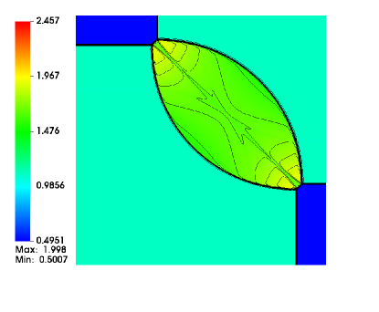
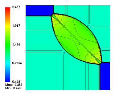
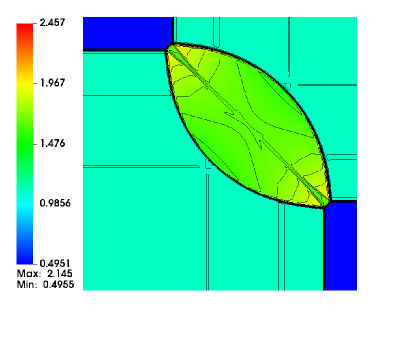
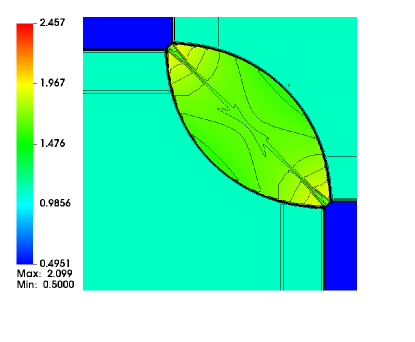
Figure 12: 2D Riemann problem (configuration 4): Density profiles at time $T=0.23$. Comparison of TeCNO4 with different reconstruction methods: (a) ENO3, (b) SP-WENO, (c) SP-WENOc, (d) DSP-WENO.

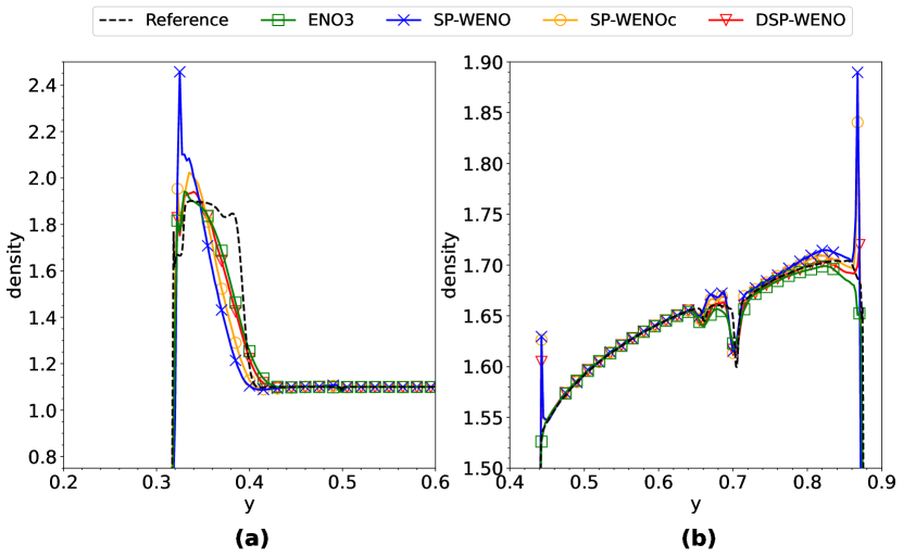
Figure 13: 2D Riemann problem (configuration 4): One-dimensional slices of the solution using each reconstruction methods: (a) $x=0.9$, (b) $x=0.5$.

2D Riemann problem (configuration 12): We consider another two-dimensional Riemann problem for the Euler equations whose initial conditions on the domain $[0,1]\times[0,1]$ are given by

$$(\rho,\text{u}_{1},\text{u}_{2},p)=\begin{cases}(0.5313,0,0,0.4)&\text{if }x>0.5,y>0.5\\ (1,0.7276,0,1)&\text{if }x\leq 0.5,y>0.5\\ (0.8,0,0,1)&\text{if }x\leq 0.5,y\leq 0.5\\ (1,0,0.7276,1)&\text{if }x>0.5,y\leq 0.5\end{cases}.$$

In this case, the evolved solution (with Neumann boundaries) comprises two shock waves and two contact discontinuities. The problem is solved on a mesh consisting of 400 $\times$ 400 cells until a final time $T=0.25$ with CFL = 0.5. As shown in Figure 14, all methods sharply resolve the shocks and contact waves. However, SP-WENO and SP-WENOc lead to significant overshoots, which can once again be observed by looking at the maximum solution values and the one-dimensional slices shown in Figure 15. On the other hand, the overshoots are generally smaller with DSP-WENO and comparable to ENO3. The reference solution is once again generated using ENO3 by solving the problem on $1200\times 1200$ mesh.

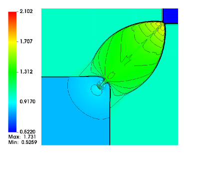
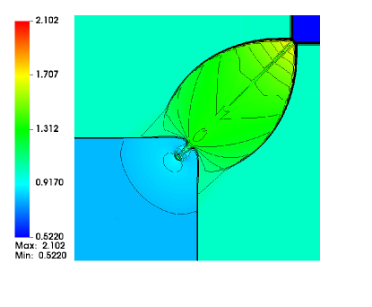
Figure 14: 2D Riemann problem (configuration 12): Density profiles at time $T=0.25$. Comparison of TeCNO4 with different reconstruction methods: (a) ENO3, (b) SP-WENO, (c) SP-WENOc, (d) DSP-WENO.

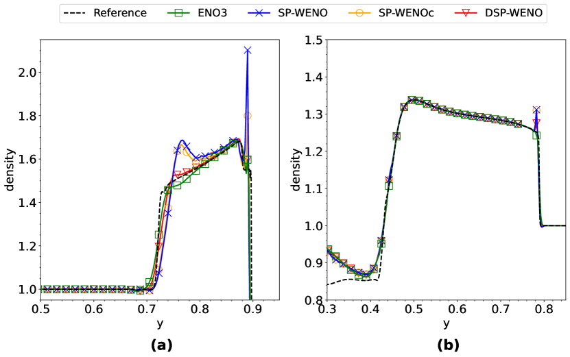
Figure 15: 2D Riemann problem (configuration 12): One-dimensional slices of the solution using each reconstruction methods: (a) $x=0.89$, (b) $x=0.5$.

Shock-vortex interaction: In this problem, we consider the interaction of a left-moving shock wave with a right-moving vortex [14]. The domain is $[0,1]\times[0,1]$, final time is $T=0.2$, and CFL = 0.45. The initial shock is given by

$${\bm{u}}_{0}(x)=\begin{cases}{\bm{u}}^{L}&\text{if }x<0.5\\ {\bm{u}}^{R}&\text{if }x\geq 0.5\end{cases},$$

where the left state is ${\bm{u}}^{L}=(\rho^{L},\text{u}_{1}^{L},\text{u}_{2}^{L},p^{L})=(1,\sqrt{\gamma},0,1)$ and the right state is given by

$$\hskip 14.22636ptp^{R} =1.3,\hskip 8.53581pt\rho^{R}=\rho^{L}\left(\frac{\gamma-1+(\gamma+1)p^{R}}{\gamma+1+(\gamma-1)p^{R}}\right),$$

$$\hskip 14.22636pt\text{u}_{1}^{R} =\sqrt{\gamma}+\sqrt{2}\left(\frac{1-p^{R}}{\sqrt{\gamma-1+p^{R}(\gamma+1)}}\right),\hskip 8.53581pt\text{u}_{2}^{R}=0.$$

A vortex is introduced into the left state by the following perturbations

$$\hskip 14.22636pt\delta\text{u}_{1} =\epsilon\frac{(y-y_{c})}{r_{c}}\exp{\left(\kappa(1-r^{2})\right)},\hskip 8.53581pt\delta\text{u}_{2}=-\epsilon\frac{(x-x_{c})}{r_{c}}\exp{\left(\kappa(1-r^{2})\right)},$$

$$\hskip 14.22636pt\delta\mathcal{T} =-\frac{\gamma-1}{4\kappa\gamma}\epsilon^{2}\exp{\left(2\kappa(1-r^{2})\right)},\hskip 8.53581pt\delta s=0.$$

where $r^{2}=((x-x_{c})^{2}+(y-y_{c})^{2})/r_{c}^{2}$. Note that the perturbation represents a steady-state isentropic vortex, whose parameters are selected to be $\epsilon=0.3$, $r_{c}=0.05$, $\kappa=0.204$, and $(x_{c},y_{c})=(0.25,0.5)$. The boundary conditions are Neumann, and the mesh consists of 400 $\times$ 400 cells. From the solutions shown in Figure 16, all methods seem to perform equally well for this test case.

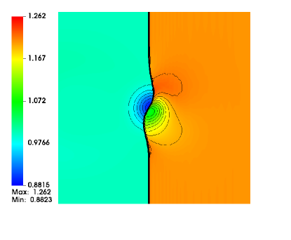
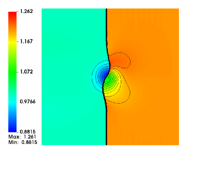
Figure 16: Shock-vortex interaction: Density profiles at time $T=0.2$. Comparison of TeCNO4 with different reconstruction methods: (a) ENO3, (b) SP-WENO, (c) SP-WENOc, (d) DSP-WENO.

6 Conclusion

In this work, we designed a novel neural network-based third-order WENO scheme called DSP-WENO, which is guaranteed to satisfy the sign property. Thus, DSP-WENO can be used within the TeCNO framework to obtain high-order entropy stable finite difference schemes. The motivation behind the proposed approach was two-fold: i) overcome the linear instability issues faced by ENO reconstruction, and ii) have better shock-capturing capabilities compared to existing WENO algorithms, i.e., SP-WENO and SP-WENOc, that satisfy the sign property.

A key element in the proposed strategy was to decouple the constraints guaranteeing the sign property and third-order accuracy (in smooth regions) from the learning process. A strong imposition of these constraints led to a convex polygonal feasible region from which the WENO weights need to be selected. Then a network was trained to adaptively choose the weights from the feasible region to ensure good reconstruction properties near discontinuities. In contrast, we could impose these constraints weakly by adding a penalty term to the loss functions (analogous to physics informed neural networks [43]). However, this would lead to the following challenges:

• The weak imposition would not guarantee the satisfaction of the sign property in all situations, thus making it impossible to prove entropy stability in the TeCNO framework.

• Neural networks trained on data extracted at a particular mesh resolution are rarely capable of demonstrating mesh convergence when tested on data from finer grids. In fact, the training (and test) errors typically plateau after a certain number of epochs, with the error values being several orders of magnitude larger than machine epsilon.

Thus, there are major benefits of decoupling such constraints from the learning process and imposing them strongly.

The training data used to train DSP-WENO did not require solving conservation laws. Instead the data was generated from a library of functions with varying smoothness, which mimic the local structures typically arising in solutions to conservation laws. Thus, the cost of generating training data is insignificant, and the trained DSP-WENO is model agnostic, i.e., does not depend on a specific conservation law. In other words, the DSP-WENO needs to be trained once offline and can then be used for any conservation law. This strategy was based on similar ideas first considered in [45] for designing troubled-cell detectors.

When comparing the numerical solutions obtained using various reconstruction methods satisfying the sign property, DSP-WENO achieved third-order accuracy in smooth regions, while being more dissipative compared to SP-WENO and SP-WENOc. This was attributed to the fact that the reconstructed jump is mostly zero (or small) with SP-WENO and SP-WENOc. However, this had a negative impact near discontinuities where the solutions exhibited large spurious oscillations due to insufficient diffusion. DSP-WENO significantly mitigated these spurious oscillations without compromising the order of accuracy in smooth regions. Further, DSP-WENO did not suffer from linear instabilities faced by ENO3. One could argue that ENO3 results in marginally better solutions near discontinuities compared to DSP-WENO. However, it is important to acknowledge that the ENO3 stencil (corresponding to an interface) comprises six cells, while SP-WENO and its variants (including DSP-WENO) have access to the solution on a stencil with just four cells.

The present work demonstrates that it is possible to use deep learning tools to learn adaptive reconstruction algorithms constrained to satisfy critical physical properties, such as the sign property. Further, it provides a framework to extend DSP-WENO to high-order ($>3$) accurate reconstructions satisfying the sign property. This would involve formulating the sign property constraint on a larger stencil and transforming the constraints into corresponding convex polyhedral regions in high dimensional spaces for the WENO weights. Thus, instead of attempting to construct an explicit weight selection strategy by hand (which presents significant challenges in high dimensions), a neural network can learn the selection procedure from training data. Further, similar sign-preserving WENO-type reconstructions can also be designed on unstructured grids. These extensions will be explored in future work.

References

- [1] Rémi Abgrall and Maria Han Veiga “Neural Network-Based Limiter with Transfer Learning” In Communications on Applied Mathematics and Computation 5.2, 2023, pp. 532–572 DOI: 10.1007/s42967-020-00087-1
- [2] Andrea Beck, David Flad and Claus-Dieter Munz “Deep neural networks for data-driven LES closure models” In Journal of Computational Physics 398, 2019, pp. 108910 DOI: https://doi.org/10.1016/j.jcp.2019.108910
- [3] Andrea D. Beck, Jonas Zeifang, Anna Schwarz and David G. Flad “A neural network based shock detection and localization approach for discontinuous Galerkin methods” In Journal of Computational Physics 423, 2020, pp. 109824 DOI: https://doi.org/10.1016/j.jcp.2020.109824
- [4] Oscar P. Bruno, Jan S. Hesthaven and Daniel V. Leibovici “FC-based shock-dynamics solver with neural-network localized artificial-viscosity assignment” In Journal of Computational Physics: X 15, 2022, pp. 100110 DOI: https://doi.org/10.1016/j.jcpx.2022.100110
- [5] Praveen Chandrashekar “Kinetic energy preserving and entropy stable finite volume schemes for compressible Euler and Navier-Stokes equations” In Communications in Computational Physics 14.5 Cambridge University Press, 2013, pp. 1252–1286
- [6] Xiaohan Cheng “A fourth order entropy stable scheme for hyperbolic conservation laws” In Entropy 21.5 MDPI, 2019, pp. 508
- [7] Xiaohan Cheng and Yufeng Nie “A third-order entropy stable scheme for hyperbolic conservation laws” In Journal of Hyperbolic Differential Equations 13.01 World Scientific, 2016, pp. 129–145
- [8] Elisabetta Chiodaroli, Camillo De Lellis and Ondřej Kreml “Global Ill-Posedness of the Isentropic System of Gas Dynamics” In Communications on Pure and Applied Mathematics 68.7, 2015, pp. 1157–1190 DOI: https://doi.org/10.1002/cpa.21537
- [9] Salvatore Cuomo et al. “Scientific Machine Learning Through Physics–Informed Neural Networks: Where we are and What’s Next” In Journal of Scientific Computing 92.3, 2022, pp. 88 DOI: 10.1007/s10915-022-01939-z
- [10] Constantine M Dafermos and Constantine M Dafermos “Hyperbolic conservation laws in continuum physics” Springer, 2005
- [11] Agnimitra Dasgupta, Javier Murgoitio-Esandi, Deep Ray and Assad Oberai “Conditional score-based generative models for solving physics-based inverse problems” In NeurIPS 2023 Workshop on Deep Learning and Inverse Problems, 2023
- [12] Tim De Ryck, Siddhartha Mishra and Deep Ray “On the approximation of rough functions with deep neural networks” In SeMA Journal 79.3, 2022, pp. 399–440 DOI: 10.1007/s40324-022-00299-w
- [13] Niccolo Discacciati, Jan S Hesthaven and Deep Ray “Controlling oscillations in high-order discontinuous Galerkin schemes using artificial viscosity tuned by neural networks” In Journal of Computational Physics 409 Elsevier, 2020, pp. 109304
- [14] Ulrik S Fjordholm, Siddhartha Mishra and Eitan Tadmor “Arbitrarily high-order accurate entropy stable essentially nonoscillatory schemes for systems of conservation laws” In SIAM Journal on Numerical Analysis 50.2 SIAM, 2012, pp. 544–573
- [15] Ulrik S Fjordholm, Siddhartha Mishra and Eitan Tadmor “ENO reconstruction and ENO interpolation are stable” In Foundations of Computational Mathematics 13 Springer, 2013, pp. 139–159
- [16] Ulrik S Fjordholm and Deep Ray “A sign preserving WENO reconstruction method” In Journal of Scientific Computing 68 Springer, 2016, pp. 42–63
- [17] Hwan Goh, Sheroze Sheriffdeen, Jonathan Wittmer and Tan Bui-Thanh “Solving Bayesian Inverse Problems via Variational Autoencoders” In Proceedings of the 2nd Mathematical and Scientific Machine Learning Conference 145, Proceedings of Machine Learning Research PMLR, 2022, pp. 386–425 URL: https://proceedings.mlr.press/v145/goh22a.html
- [18] Sigal Gottlieb, Chi-Wang Shu and Eitan Tadmor “Strong stability-preserving high-order time discretization methods” In SIAM review 43.1 SIAM, 2001, pp. 89–112
- [19] Ayoub Gouasmi, Scott M. Murman and Karthik Duraisamy “Entropy Conservative Schemes and the Receding Flow Problem” In Journal of Scientific Computing 78.2, 2019, pp. 971–994 DOI: 10.1007/s10915-018-0793-8
- [20] Amiram Harten “On the symmetric form of systems of conservation laws with entropy” In Journal of Computational Physics 49.1, 1983, pp. 151–164 DOI: https://doi.org/10.1016/0021-9991(83)90118-3
- [21] Daniel Zhengyu Huang, Nicholas H. Nelsen and Margaret Trautner “An operator learning perspective on parameter-to-observable maps”, 2024 arXiv:2402.06031 [cs.LG]
- [22] Farzad Ismail and Philip L. Roe “Affordable, entropy-consistent Euler flux functions II: Entropy production at shocks” In Journal of Computational Physics 228.15, 2009, pp. 5410–5436 DOI: https://doi.org/10.1016/j.jcp.2009.04.021
- [23] Guang-Shan Jiang and Chi-Wang Shu “Efficient Implementation of Weighted ENO Schemes” In Journal of Computational Physics 126.1, 1996, pp. 202–228 DOI: https://doi.org/10.1006/jcph.1996.0130
- [24] Patrick Kidger and Terry Lyons “Universal Approximation with Deep Narrow Networks” In Proceedings of Thirty Third Conference on Learning Theory 125, Proceedings of Machine Learning Research PMLR, 2020, pp. 2306–2327 URL: https://proceedings.mlr.press/v125/kidger20a.html
- [25] Diederik P Kingma and Jimmy Ba “Adam: A method for stochastic optimization” In arXiv preprint arXiv:1412.6980, 2014
- [26] Tatiana Kossaczká, Matthias Ehrhardt and Michael Günther “Enhanced fifth order WENO shock-capturing schemes with deep learning” In Results in Applied Mathematics 12 Elsevier, 2021, pp. 100201
- [27] S.. Kružkov “First order quasilinear equations in several independent variables” In Mathematics of the USSR-Sbornik 10.2, 1970, pp. 217 DOI: 10.1070/SM1970v010n02ABEH002156
- [28] Alexander Kurganov and Eitan Tadmor “Solution of two-dimensional Riemann problems for gas dynamics without Riemann problem solvers” In Numerical Methods for Partial Differential Equations: An International Journal 18.5 Wiley Online Library, 2002, pp. 584–608
- [29] Peter D Lax “Weak solutions of nonlinear hyperbolic equations and their numerical computation” In Communications on pure and applied mathematics 7.1 Wiley Online Library, 1954, pp. 159–193
- [30] Philippe G Lefloch, Jean-Marc Mercier and Christian Rohde “Fully discrete, entropy conservative schemes of arbitrary order” In SIAM Journal on Numerical Analysis 40.5 SIAM, 2002, pp. 1968–1992
- [31] Camillo Lellis and László Székelyhidi “On Admissibility Criteria for Weak Solutions of the Euler Equations” In Archive for Rational Mechanics and Analysis 195.1, 2010, pp. 225–260 DOI: 10.1007/s00205-008-0201-x
- [32] Yue Li, Lin Fu and Nikolaus A Adams “A six-point neuron-based ENO (NENO6) scheme for compressible fluid dynamics” In arXiv preprint arXiv:2207.08500, 2022
- [33] Zongyi Li et al. “Fourier Neural Operator for Parametric Partial Differential Equations” arXiv, https://arxiv.org/abs/2010.08895, 2020 DOI: 10.48550/ARXIV.2010.08895
- [34] Timur Linde, Philip Roe, Timur Linde and Philip Roe “Robust euler codes” In 13th computational fluid dynamics conference, 1997, pp. 2098
- [35] Lu Lu et al. “Learning nonlinear operators via DeepONet based on the universal approximation theorem of operators” In Nature Machine Intelligence 3.3, 2021, pp. 218–229 DOI: 10.1038/s42256-021-00302-5
- [36] Kjetil O Lye, Siddhartha Mishra, Deep Ray and Praveen Chandrashekar “Iterative surrogate model optimization (ISMO): An active learning algorithm for PDE constrained optimization with deep neural networks” In Computer Methods in Applied Mechanics and Engineering 374 Elsevier, 2021, pp. 113575
- [37] Kjetil O. Lye, Siddhartha Mishra and Deep Ray “Deep learning observables in computational fluid dynamics” In Journal of Computational Physics 410, 2020, pp. 109339 DOI: https://doi.org/10.1016/j.jcp.2020.109339
- [38] Romit Maulik, Omer San and Jamey D. Jacob “Spatiotemporally dynamic implicit large eddy simulation using machine learning classifiers” In Physica D: Nonlinear Phenomena 406, 2020, pp. 132409 DOI: https://doi.org/10.1016/j.physd.2020.132409
- [39] Prashant Kumar Pandey and Ritesh Kumar Dubey “Sign stable arbitrary high order reconstructions for constructing non-oscillatory entropy stable schemes” In Applied Mathematics and Computation 454 Elsevier, 2023, pp. 128099
- [40] Dhruv Patel et al. “Variationally mimetic operator networks” In Computer Methods in Applied Mechanics and Engineering 419, 2024, pp. 116536 DOI: https://doi.org/10.1016/j.cma.2023.116536
- [41] Dhruv V Patel, Deep Ray and Assad A Oberai “Solution of physics-based Bayesian inverse problems with deep generative priors” In Computer Methods in Applied Mechanics and Engineering 400 Elsevier, 2022, pp. 115428
- [42] Allan Pinkus “Approximation theory of the MLP model in neural networks” In Acta Numerica 8 Cambridge University Press, 1999, pp. 143–195 DOI: 10.1017/S0962492900002919
- [43] M. Raissi, P. Perdikaris and G.E. Karniadakis “Physics-informed neural networks: A deep learning framework for solving forward and inverse problems involving nonlinear partial differential equations” In Journal of Computational Physics 378, 2019, pp. 686–707 DOI: https://doi.org/10.1016/j.jcp.2018.10.045
- [44] Deep Ray “A Third-Order Entropy Stable Scheme for the Compressible Euler Equations” In Theory, Numerics and Applications of Hyperbolic Problems II: Aachen, Germany, August 2016, 2018, pp. 503–515 Springer
- [45] Deep Ray and Jan S Hesthaven “An artificial neural network as a troubled-cell indicator” In Journal of computational physics 367 Elsevier, 2018, pp. 166–191
- [46] Deep Ray and Jan S Hesthaven “Detecting troubled-cells on two-dimensional unstructured grids using a neural network” In Journal of Computational Physics 397 Elsevier, 2019, pp. 108845
- [47] Deep Ray, Javier Murgoitio-Esandi, Agnimitra Dasgupta and Assad A. Oberai “Solution of physics-based inverse problems using conditional generative adversarial networks with full gradient penalty” A Special Issue in Honor of the Lifetime Achievements of T. J. R. Hughes In Computer Methods in Applied Mechanics and Engineering 417, 2023, pp. 116338 DOI: https://doi.org/10.1016/j.cma.2023.116338
- [48] AM Rogerson and E Meiburg “A numerical study of the convergence properties of ENO schemes” In Journal of Scientific Computing 5 Springer, 1990, pp. 151–167
- [49] Lukas Schwander, Deep Ray and Jan S. Hesthaven “Controlling oscillations in spectral methods by local artificial viscosity governed by neural networks” In Journal of Computational Physics 431, 2021, pp. 110144 DOI: https://doi.org/10.1016/j.jcp.2021.110144
- [50] Chi-Wang Shu and Stanley Osher “Efficient implementation of essentially non-oscillatory shock-capturing schemes, II” In Journal of Computational Physics 83.1 Elsevier, 1989, pp. 32–78
- [51] Anand Pratap Singh and Karthik Duraisamy “Using field inversion to quantify functional errors in turbulence closures” In Physics of Fluids 28.4, 2016, pp. 045110 DOI: 10.1063/1.4947045
- [52] Ben Stevens and Tim Colonius “Enhancement of shock-capturing methods via machine learning” In Theoretical and Computational Fluid Dynamics 34.4, 2020, pp. 483–496 DOI: 10.1007/s00162-020-00531-1
- [53] Eitan Tadmor “Entropy stability theory for difference approximations of nonlinear conservation laws and related time-dependent problems” In Acta Numerica 12 Cambridge University Press, 2003, pp. 451–512
- [54] Eleuterio F Toro “Riemann solvers and numerical methods for fluid dynamics: a practical introduction” Springer Science & Business Media, 2013
- [55] Andrew R. Winters and Gregor J. Gassner “Affordable, entropy conserving and entropy stable flux functions for the ideal MHD equations” In Journal of Computational Physics 304, 2016, pp. 72–108 DOI: https://doi.org/10.1016/j.jcp.2015.09.055
- [56] Liu Yang, Dongkun Zhang and George Em Karniadakis “Physics-Informed Generative Adversarial Networks for Stochastic Differential Equations” In SIAM Journal on Scientific Computing 42.1, 2020, pp. A292–A317 DOI: 10.1137/18M1225409
- [57] Dmitry Yarotsky and Anton Zhevnerchuk “The phase diagram of approximation rates for deep neural networks” arXiv, https://arxiv.org/abs/1906.09477, 2019 DOI: 10.48550/ARXIV.1906.09477
- [58] Jonas Zeifang and Andrea Beck “A data-driven high order sub-cell artificial viscosity for the discontinuous Galerkin spectral element method” In Journal of Computational Physics 441, 2021, pp. 110475 DOI: https://doi.org/10.1016/j.jcp.2021.110475