Extrapolating Solution Paths of Polynomial Homotopies
towards Singularities with PHCpack and phcpy

Abstract

A robust path tracker [Telen, Van Barel, Verschelde, SISC 2020] computes the radius of convergence of Newton’s method, estimates the distance to the nearest path, and then applies Padé approximants to predict the next point on the path. Apriori step size control is less sensitive to finely tuned tolerances than aposteriori step size control, and is therefore robust. Extrapolation methods are effective to accurately locate the singular points at the end of solution paths, as illustrated with phcpy, the scripting interface to PHCpack.

1 Introduction

A polynomial homotopy is a family of polynomial systems which depend on one parameter $t$. Regular solutions of a polynomial homotopy have Taylor series developments in $t$. The solutions paths are analytic functions of $t$. Application of the theorem of Fabry [4] enables to locate the nearest singular solution. The calculations in this paper can be considered in the area of numerical analytic continuation [6], [18, 19].

Extrapolation methods, in particular the rho [26] and theta [2] algorithms, are effective in accelerating logarithmically converging series towards a single pole of a polynomial homotopy. We demonstrate the interplay between compiled code in a library, for the computationally intensive calculation of the Taylor series, and the interactive Python scripts for the extrapolation methods. Our calculations happen in Jupyter notebooks [11] with phcpy [16, 21] in a Python kernel. The interface to the compiled code in PHCpack [20] does not require compilation as it is done through the Ctypes module of Python which allows to call functions in libraries directly, similar to ccall in Julia.

Since version 2.4.88, PHCpack became a crate of alire, the package manager of the gnu-ada compiler, which builds the executable phc and libPHCpack, integrating code of MixedVol [5] and DEMiCs [14], for fast mixed volume computation, and algorithms for multiple double arithmetic of QDlib [7] and CAMPARY [9]. The development of phcpy was motivated in part by SageMath [3]. All software is free and open source, released under version 3 of the GNU GPL license. Computations are done with phcpy 1.1.4 and version 2.4.90 of PHCpack.

2 Extrapolation Experiments

The polynomial homotopy

$$x^{2}-\frac{4}{5}\left(\frac{1}{2}-I\right)\left(\vphantom{\frac{1}{2}}1-t\right)\left(\frac{1}{2}+I-t\right)=0,\quad I=\sqrt{-1}.$$ (1)

has two singularities: one at $t=1$ and another at $t=1/2+I$. The coefficient $4/5(1/2-I)$ makes that at $t=0$, the solution paths $x(t)$ start at $x(0)=\pm~{}1$. The phase portrait [24], made with complexplorer-0.1.2 [13] (which depends on matplotlib [8]), is shown in Figure 1.

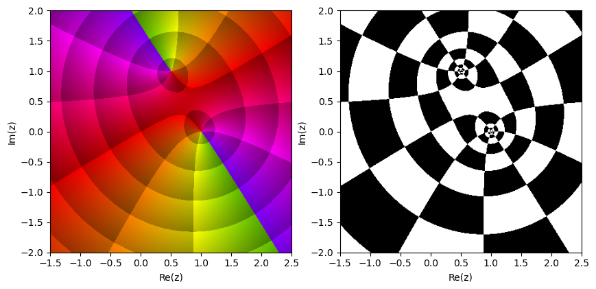
Figure 1: A phase portrait of $f(z)=\sqrt{4/5(1/2-I)(1-z)(1/2+I-z)}$, depicting at the left the color-coded phase $f/|f|$ on the domain of $f$. At the right is a polar chessboard.

Using the algorithms in [1] to compute the Taylor series is done with phcpy in the code snippet below:

from phcpy.solutions import make_solution
from phcpy.series import double_newton_at_point

pol = [’x^2 - (4/5)*(1/2 - I)*(1 - t)*(1/2 + I - t);’]
variables = [’x’, ’t’]
sols = [make_solution(variables, [1, 0])]
deg = 33  # degree of truncation
nit = 8   # number of iterations of Newton’s method
srs = double_newton_at_point(pol, sols, idx=2, maxdeg=deg, nbr=nit)

The srs contains the string representation of the Taylor series and the coefficients can be extracted with the help of SymPy [10]. Denoting $c_{n}$ as the coefficient of $t^{n}$ in the Taylor series, the ratio $c_{n}/c_{n+1}$ equals (1.0362677867627397 -0.03656143770249911j), for $n=31$, illustrating the very slow convergence to 1. Series such as this are said to be converge logarithmically, as it may take about twice as many terms in the series to gain one bit of accuracy.

The rho algorithm of Wynn [26] performs spectacularly well on the Taylor series of $x(t)=\sqrt{1-t}$, where there is only one pole. In the definition of the function rhoComplex below, observe the inverse divided differences. The connection with Thiele interpolation is one possible justification of its good performance on $x(t)=\sqrt{1-t}$.

def rhoComplex(nbr):
    """
    Runs the rho algorithm in complex double arithmetic,
    on the numbers given in the list nbr, using x(n) = n+1.
    Returns the last element of the table of extrapolated numbers.
    """
    rho1 = [1.0/(nbr[n] - nbr[n-1]) for n in range(1, len(nbr))]
    rho = [nbr, rho1]
    for k in range(2, len(nbr)):
        nextrho = []
        for n in range(k, len(nbr)):
            invrho1 = complex(k)/(rho[k-1][n-k+1] - rho[k-1][n-k])
            nextrho.append(rho[k-2][n-k+1] + invrho1)
        rho.append(nextrho)
    return nextrho[-1]

Because the two singularities of (1) are relatively too close to each other, the rho algorithm fails to improve the sequence of Fabry ratios. In the second homotopy:

$$x^{2}-\left(\frac{1}{272}\right)\left(\vphantom{\frac{1}{2}}-4-16I\right)\left(\vphantom{\frac{1}{2}}1-t\right)\left(\vphantom{\frac{1}{2}}-4+16I-t\right)=0,$$ (2)

the singularity at $-4+16I$ is much farther from the other singularity at $1$, and then the rho algorithm ends at (1.0000000000014202+4.354118985724171e-14j), using 32 coefficients of the Taylor series, with an error of 1.42e-12.

The differences between the location of the singularities in the homotopies (1) and (2) is shown in the schematic of Figure 2. The $P$ at the right of Figure 2 illustrates the notion of the last pole, introduced in [23].

Figure 2: At the left, the pole $P=1/2+I$ is relatively close to 1, while at the right, the pole $P=-4+16I$ is much farther from 1.

The right of Figure 2 is a representative schematic for a solution path converging to a singular solution at 1.

3 Path Tracking Towards a Singular Solution

One important innovation in the modernization [21] of PHCpack with a scripting interface was the introduction of a step-by-step path tracker, which allows the user to ask for the next point on a path. Recently, another step-by-step tracker which applies the apriori step size control algorithms of [17] was added to phcpy.

The homotopy

$$\gamma(1-t)\left(\begin{array}[]{rcl}x^{2}-1&=&0\\ y^{2}-1&=&0\\ \end{array}\right)+t\left(\begin{array}[]{rcl}x^{2}+y-3&=&0\\ x+0.125y^{2}-1.5&=&0\end{array}\right)$$ (3)

ends at $t=1$ at an example of [15], which has a triple root at $(x,y)=(1,2)$. Figure 3 shows one path defined by the homotopy (3), converging to $(1,2)$.

Figure 3: Points on one solution path starting at $(1,1)$ and converging to $(1,2)$.

The code below collects the points on the solution path in the list path. The constant $\gamma$ in the homotopy (3) is set to the value $-0.917-0.398I$. Expecting a singularity at the end of the path, as long as the distance between the closest pole and 1.0 is larger than 1.0e-4, the path tracker continues. Three lists are produced: in path are the points on the path, in predicted are the predicted solutions, and poles contains the list of poles closest to the path.

from phcpy.solutions import make_solution
from phcpy.curves import set_gamma_constant
from phcpy.curves import initialize_double_artificial_homotopy
from phcpy.curves import set_double_solution, get_double_solution
from phcpy.curves import double_predict_correct, double_t_value
from phcpy.curves import double_closest_pole

pols = [’x**2+y-3;’, ’x+0.125*y**2-1.5;’]
start = [’x**2 - 1;’, ’y**2 - 1;’]
startsol = make_solution([’x’, ’y’], [1, 1])
set_gamma_constant(complex(-0.917, -0.398))
initialize_double_artificial_homotopy(pols, start)
set_double_solution(2, startsol)
path = [startsol]
predicted = []
poles = []
cfp = complex(0.0)
while abs(cfp - 1.0) > 1.0e-4:
    double_predict_correct()
    (repole, impole) = double_closest_pole()
    tval = double_t_value()
    cfp = complex(tval + repole, impole)
    poles.append(cfp)
    sol = get_double_solution()
    predsol = get_double_predicted_solution()
    path.append(sol)
    predicted.append(predsol)
print(sol)

The code prints

    t :  9.99968379127468E-01   0.00000000000000E+00
    m : 1
    the solution for t :
     x :  1.05353846638456E+00   6.88135807075172E-03
     y :  1.89010705713382E+00  -1.44977473137858E-02
    == err :  6.369E-14 = rco :  7.184E-04 = res :  2.849E-17 =

The value 7.184E-04 next to rco is the estimate for the inverse condition number of the Jacobian matrix at the point, which gives an upper bound on the error of the update in Newton’s method. In particular, the update of Newton’s method is correct up to the last four decimal places. Even as 0.999684 is already close to 1, the solution is thus still well conditioned.

The list poles ends with (1.0000808949264557-6.886127445687259e-08j). Observe how small the imaginary part is. Only seven terms in the Taylor series were used to compute this approximation for 1.0.

To visualize the poles with complexplorer, consider the function

$$f(z)=\sum_{p\in L}\frac{1}{z-p},$$ (4)

where $L$ is the list of the first twelve poles. The phase portrait of $f$ is shown in Figure 4. The phase portrait starts to look interesting at the first closest pole, around $t\approx 0.471+0.101I$.

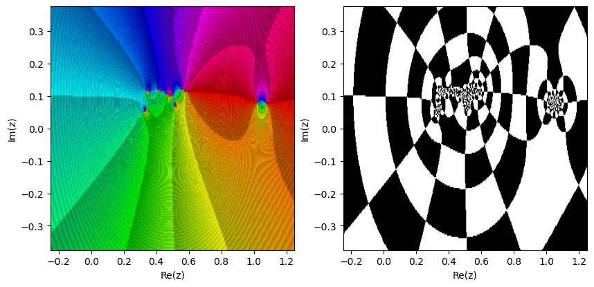
Figure 4: A phase portrait of $f(z)$, defined in (4) by the poles of one path converging to a singular solution.

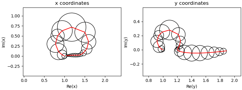
Figure 5: At each point on the path, a circle is drawn, with center at the point and the radius is the distance to the predicted solution.

Figure 5 is constructed using the information of the points on the path and the predicted solutions. The predicted solutions are evaluated Padé approximants, evaluated in the radius of convergence for Newton’s method, as estimated by the application of the theorem of Fabry. The plots in Figure 5 show a sequence of circles with overlapping interiors. Towards the end of the path, observe that the radii of the circles decrease, as we approach the singularity at the end. The smaller circles in the middle of the path indicate nearby poles.

4 Iterated Aitken Extrapolation

Looking at the list path, the solution at the end is not very accurate: the 1-norm of its solution components equals 2.27e-01, which means that we have only one decimal place of accuracy. If we consider the last seven points on the path, then we observe a very slowly converging sequence of points. Aitken extrapolation is effective in accelerating logarithmically converging sequences [12]. The function below contains the definition of Aitken extrapolation:

     def Aitken(x):
         """
         Applies Aitken extrapolation to the sequence x.
         Returns the transformed sequence.
         """
         y = [0.0 for _ in range(len(x)-2)]
         for k in range(len(x)-2):
             dxk = x[k+1] - x[k]
             ddx = x[k+2] - 2*x[k+1] + x[k]
             y[k] = x[k] - dxk*dxk/ddx
         return y

The iterated Aitken extrapolation applies Aitken extrapolation repeatedly [25], as defined in the function below:

def repeatedAitken(x, exa, verbose=True):
    """
    Applies Aitken extrapolation repeatedly on the sequence x.
    If verbose, then the error with the exact value in exa is shown.
    Returns the last element.
    """
    cffs = x
    while len(cffs) > 2:
        a = Aitken(cffs)
        if verbose:
            print(’on’, len(cffs), ’:’, a[len(a)-1], end=’’)
            err = abs(a[len(a)-1] - exa)
            print(f’ error :{err: .2e}’)
        cffs = a
    return cffs[0]

Executing repeatedAitken(ypt, 2.0) produces the sequence

on 7 : (2.0137784911225802+0.004510752594407998j) error : 1.45e-02
on 5 : (2.0026132752890415+0.001430742263173204j) error : 2.98e-03
on 3 : (2.0008714460040284+0.000612101736300566j) error : 1.06e-03

with similar results as repeatedAitken(xpt, 1.0). The error has decreased from 2.27e-01 to 1.69e-03. With relatively little effort, we gained two decimal places in the solution.

The rho algorithm and its iterated version produce similar results, but its application is more delicate, as the default values of the interpolation points need to take the values of the $t$ parameter into account.

5 Building and Installing phcpy

Thanks to the efforts of Doug Torrance, both PHCpack and phcpy can be installed with the package managers of Ubuntu.

Ad hoc makefiles, customized for Linux, Windows, and Mac OS X, were written during the development of PHCpack, but became too cumbersome to maintain. GPRbuild is the project manager of the GNAT toolchain, which made the building of the executable phc and the library libPHCpack, along with its components in C and C++ (in particular: DEMiCs) more portable, since version 2.4.85 [22]. Since version 2.4.88, PHCpack can be built via "alr get phcpack".

The development of phcpy started in python2, with the writing of extension modules, which needed compilation, and later adjustments for python3. The compilation imposed restrictions for Windows, as the Python interpreters on Windows are typically built with the Microsoft compilers which are not interoperable with gcc. Version 1.1.3 of phcpy (the third major rewrite of phcpy) used the Ctypes module. Once the libPHCpack is in its proper place, the instruction "pip install ." in the folder where the setup.py is located will extend the Python interpreter with phcpy, also on native Windows systems.

6 Conclusions

Extrapolating on Taylor series towards singular solutions, this paper illustrates the application of numerical analytic continuation to solving polynomial systems. With phcpy, the algorithms of [17] and [23] have become better accessible.

References

- [1] N. Bliss and J. Verschelde. The method of Gauss-Newton to compute power series solutions of polynomial homotopies. Linear Algebra and its Applications, 542:569–588, 2018.
- [2] C. Brezinski. Accélération de suites à convergence logarithmique. C. R. Acad. Sc. Paris, Série A, 273:727–730, 1971.
- [3] B. Eröcal and W. Stein. The Sage project: Unifying free mathematical software to create a viable alternative to Magma, Maple, Mathematica, and MATLAB. In K. Fukuda, J. van der Hoeven, M. Joswig, and N. Takayama, editors, Mathematical Software - ICMS 2010, volume 6327 of Lecture Notes in Computer Science, pages 12–27. Springer-Verlag, 2010.
- [4] E. Fabry. Sur les points singuliers d’une fonction donnée par son développement en série et l’impossibilité du prolongement analytique dans des cas très généraux. Annales scientifiques de l’École Normale Supérieure, 13:367–399, 1896.
- [5] T. Gao, T. Y. Li, and M. Wu. Algorithm 846: MixedVol: a software package for mixed-volume computation. ACM Trans. Math. Softw., 31(4):555–560, 2005.
- [6] P. Henrici. An algorithm for analytic continuation. SIAM Journal on Numerical Analysis, 3(1):67–78, 1966.
- [7] Y. Hida, X. S. Li, and D. H. Bailey. Algorithms for quad-double precision floating point arithmetic. In 15th IEEE Symposium on Computer Arithmetic (Arith-15 2001), pages 155–162. IEEE Computer Society, 2001.
- [8] J. D. Hunter. Matplotlib: A 2D graphics environment. Computing in Science & Engineering, 9(3):90–95, 2007.
- [9] M. Joldes, J.-M. Muller, V. Popescu, and Tucker. W. CAMPARY: Cuda Multiple precision arithmetic library and applications. In Mathematical Software – ICMS 2016, the 5th International Conference on Mathematical Software, pages 232–240. Springer-Verlag, 2016.
- [10] D. Joyner, O. Čertík, A. Meurer, and B. E. Granger. Open source computer algebra systems: SymPy. ACM Communications in Computer Algebra, 45(4):225–234, 2011.
- [11] T. Kluyver, B. Ragan-Kelley, F. Pérez, B. Granger, M. Bussonnier, J. Frederic, K. Kelley, J. Hamrick, J. Grout, S. Corlay, P. Ivanov, D. Avila, S. Abdalla, C. Willing, and Jupyter Development Team. Jupyter Notebooks—a publishing format for reproducible computational workflows. In F. Loizides and B. Schmidt, editors, Positioning and Power in Academic Publishing: Players, Agents, and Agendas, pages 87–90. IOS Press, 2016.
- [12] C. Kowaleski. Acceleration de la convergence pour certaines suites a convergence logarithmique. In M.G. de Bruin and H. van Rossum, editors, Padé Approximation and its Applications, Amsterdam 1980, volume 888 of Lecture Notes in Mathematics, pages 263–272. Springer-Verlag, 1981.
- [13] I. Kuvychko. Complexplorer. Available at https://github.com/kuvychko/ complexplorer.
- [14] T. Mizutani and A. Takeda. DEMiCs: A software package for computing the mixed volume via dynamic enumeration of all mixed cells. In M.E. Stillman, N. Takayama, and J. Verschelde, editors, Software for Algebraic Geometry, volume 148 of The IMA Volumes in Mathematics and its Applications, pages 59–79. Springer-Verlag, 2008.
- [15] T. Ojika. Modified deflation algorithm for the solution of singular problems. I. A system of nonlinear algebraic equations. Journal of Mathematical Analysis and Applications, 123:199–221, 1987.
- [16] J. Otto, A. Forbes, and J. Verschelde. Solving polynomial systems with phcpy. In Proceedings of the 18th Python in Science Conference, pages 563–582, 2019.
- [17] S. Telen, M. Van Barel, and J. Verschelde. A robust numerical path tracking algorithm for polynomial homotopy continuation. SIAM Journal on Scientific Computing, 42(6):A3610–A3637, 2020.
- [18] L. N. Trefethen. Approximation Theory and Approximation Practice. Extented Edition. SIAM, 2020.
- [19] L. N. Trefethen. Numerical analytic continuation. Japan Journal of Industrial and Applied Mathematics, 40(3):1587–1636, 2023.
- [20] J. Verschelde. Algorithm 795: PHCpack: A general-purpose solver for polynomial systems by homotopy continuation. ACM Trans. Math. Softw., 25(2):251–276, 1999. Available at https://github.com/janverschelde/PHCpack.
- [21] J. Verschelde. Modernizing PHCpack through phcpy. In P. de Buyl and N. Varoquaux, editors, Proceedings of the 6th European Conference on Python in Science (EuroSciPy 2013), pages 71–76, 2014.
- [22] J. Verschelde. Exporting Ada software to Julia and Python. Ada User Journal, 43(1):75–77, 2022.
- [23] J. Verschelde and K. Viswanathan. Locating the closest singularity in a polynomial homotopy. In Proceedings of the 24th International Workshop on Computer Algebra in Scientific Computing (CASC 2022), volume 13366 of Lecture Notes in Computer Science, pages 333–352. Springer-Verlag, 2022.
- [24] E. Wegert. Visual Complex Functions: An Introduction with Phase Portraits. Birkhäuser, 2012.
- [25] E.J. Weniger. Nonlinear sequence transformations for the acceleration of convergence and the summation of series. Computer Physics Reports, 10:189–371, 1989.
- [26] P. Wynn. On a procrustean technique for the numerical transformation of slowly convergent sequences and series. Proc. Camb. Phil. Soc., 52:663–672, 1956.