Deep Clustering Evaluation: How to Validate Internal Clustering Validation Measures
Abstract
Deep clustering, a method for partitioning complex, high-dimensional data using deep neural networks, presents unique evaluation challenges. Traditional clustering validation measures, designed for low-dimensional spaces, are problematic for deep clustering, which involves projecting data into lower-dimensional embeddings before partitioning. Two key issues are identified: 1) the curse of dimensionality when applying these measures to raw data, and 2) the unreliable comparison of clustering results across different embedding spaces stemming from variations in training procedures and parameter settings in different clustering models. This paper addresses these challenges in evaluating clustering quality in deep learning. We present a theoretical framework to highlight ineffectiveness arising from using internal validation measures on raw and embedded data and propose a systematic approach to applying clustering validity indices in deep clustering contexts. Experiments show that this framework aligns better with external validation measures, effectively reducing the misguidance from the improper use of clustering validity indices in deep learning.
Keywords: Deep clustering, Internal validation measures, Clustering evaluation, ACE, Admissible space
1 Introduction
Clustering, a core task in unsupervised learning, groups entities based on similarities, proving essential across various applications from image analysis to data segmentation (LeCun et al.,, 1998; JAIN et al.,, 1999). With advancements in deep learning, particularly in image processing, deep networks have excelled in label prediction and feature extraction from unlabeled data. This progress has spawned deep clustering methods (Yang et al.,, 2016; Ghasedi Dizaji et al.,, 2017; Caron et al.,, 2018), which enhance traditional clustering techniques’ scalability to high-dimensional data by using deep networks to project data into a lower-dimensional latent feature space (or named embedding space). This projection facilitates data partitioning in this more manageable space, supported by innovative clustering loss designs and network structures, leading to a proliferation of successful clustering methods in diverse fields.
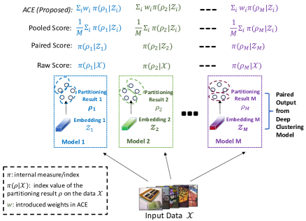
Evaluating clustering results in machine learning is essential for ensuring algorithmic quality and optimal partitioning. This evaluation typically involves two types (Liu et al.,, 2010): internal measures (also known as validity index), which assess clustering quality based on the data and outcomes without external information, and external measures, which compare results to known labels or “ground truth”. The usage of external measures is often limited as such ground truth is frequently unavailable. See more details in Section 2.2. Internal measures often falter for high-dimensional data due to the notorious curse of dimensionality, making their application based on the raw input data (the generated score from which is referred to as the raw score in this paper) impractical for the majority of deep clustering problems. In addition to the data partitioning results, deep clustering algorithms yield embedded data, constituting a “paired output” alongside the partitioning results. Due to the significantly reduced dimensionality of the embedded data, many works in the literature (Wang et al.,, 2018, 2021; Huang et al.,, 2021b, a; Ronen et al.,, 2022; Hadipour et al.,, 2022; Li et al.,, 2023) utilize internal measures based on the paired embedded data as a validation criterion (referred to as the paired score in this paper). Figure 1 illustrates these two evaluation approaches. Despite the ability of embedded data to mitigate the curse of dimensionality, the application of the paired score for calculating and comparing different partitioning results is problematic. The embedding space, where this embedded data resides, is influenced by training parameters and processes. Internal measures are typically designed under the assumption that the evaluated data comes from the same feature space. Consequently, this variation in embedding spaces hampers the precise reflection of partitioning quality and compromises the reliability of comparing internal measure values for partitioning results based on their respective paired embedding spaces. For instance, one model might disperse embedded data points across clusters with more separation but slight errors at the boundaries, while another could distribute data across clusters more compactly without any errors in classification. Despite its less precise partitioning, the first model might receive a higher score from an internal measure like the silhouette score, which evaluates based on distances within and between clusters. The questionable reliance on the paired score in much of the existing literature, as mentioned earlier, highlights the need to appropriately validate internal measures for assessing deep clustering performances. This paper provides a theoretical understanding that such comparisons across different embedding spaces may fail due to the embedding space discrepancy. Ideally, we want to compare clustering results based on one ideal embedding space. However, in real practice, we lack knowledge about which space is ideally separable. To address this problem, we propose a simple yet effective logic and strategy to guide the usage of internal measures in deep clustering evaluation.
In summary, our major contributions include:
Theoretical Justifications: We provide formal theoretical proofs showcasing that employing both 1) the high-dimensional raw data and 2) separate embedded data paired with individual partitioning results for computing clustering validity measures does not ensure the convergence of the comparative relationship between clustering results to the truth. We also establish theoretical properties for identifying admissible embedding spaces among all embedding spaces obtained with clustering results. These properties serve as a foundational framework for developing a strategy to select optimal spaces. To the best of our knowledge, we are the first to explore the significance of feature spaces for evaluating deep clustering.
Evaluation Strategy: Based on the theoretical analysis, we introduce a strategy for identifying admissible embedding spaces during evaluation. By combining the calculated internal measure scores from the chosen embedding spaces, we enhance the robustness of the evaluation results. Through extensive experiments and ablation studies, focusing on scenarios such as hyperparameter tuning, cluster number selection, and checkpoint selection, we demonstrate the effectiveness and importance of the proposed framework for evaluating deep clustering methods.
2 Preliminaries
2.1 Deep Clustering
Let denote a collection of unlabeled observations, where is i.i.d. generated from some unknown distribution . A clustering problem can be defined as partitioning these observations into latent groups or clusters. We denote the unknown labels corresponding to the observations as , where each and represents the number of the groups. Clustering techniques find a good mapping (up to permutations) from to , which we represent as . The outcomes of form a partition of the index set , where if and only if for any and . Deep clustering approaches transform the high-dimensional space to a significantly lower-dimensional space through an encoder network, denoted as , that maps each to . The reduced-dimension data space is often referred to in the literature as embedding space. In practice, can be built using a convnet or transformer encoder. Subsequently, clustering is performed on the lower-dimensional data to generate labels . In this context, we employ to represent the mapping from to . Then the clustering algorithm can be expressed as a composition function . Generally, existing deep clustering methods can be categorized into two classes: autoencoder-based and clustering deep neural network-based approaches (Min et al.,, 2018). Please refer to Appendix A.1 for an in-depth literature review and additional details on various deep clustering methods.
2.2 Clustering Evaluation
External measures
In clustering, partitions are autonomously learned without supervised labels, hindering a direct comparison with the actual partition on holdout sets, as commonly practiced in supervised learning. If true partition labels are available, external validation measures, which assess the similarity between estimated partition labels and true cluster labels, are employed. Two widely used metrics for this purpose are normalized mutual information (NMI) and clustering accuracy (ACC) (see Appendix A.3 for definitions). External measures are primarily used for benchmarking, but their applicability is limited in many clustering evaluation settings due to the requirement for true labels. Despite its limited usage, considering it as a similarity measure with truth, in this paper, we will treat it as the “truth” measure in our analysis.
Internal measures
Internal measures, known as validity indices, are developed to evaluate clustering quality based on the intrinsic characteristics of data and the resulting partitions, without relying on external labels. Examples of these indices include the Silhouette score (Rousseeuw,, 1987), Calinski-Harabasz index (Caliński & Harabasz,, 1974), Davies-Bouldin index (Davies & Bouldin,, 1979), Cubic clustering criterion (CCC) (Sarle,, 1983), Dunn index (Dunn,, 1974), Cindex (Hubert & Levin,, 1976), SDbw index (Halkidi & Vazirgiannis,, 2001), and CDbw index (Halkidi & Vazirgiannis,, 2008). Given the data and a resulting partition , we use the notation to indicate the clustering validity index. Since the focus in this paper is on the embedding space, we use to represent , which denotes the score based on the embedded data . For a comprehensive understanding of each index, including definitions and details, please refer to Appendix A.4.
3 Theoretical Analysis for Deep Clustering Evaluation
Given the established preliminaries, in this section, we provide a theoretical analysis for deep clustering evaluation. The proofs substantiating the theorems and corollaries are available in Appendix A.2 for further reference.
Lemma 1.
[Theorem 1 in Beyer et al., (1999)] Denote random points where each point is a -dimensional vector. Let be a random query point that is chosen independently from . Let be the probability density function of any fixed distribution on . For any distance function , define and . Given a fixed , for any , we have
where the expectation is taken over the product distribution .
Theorem 1.
[Distance Meaningless in High Dimensions] The clustering validity index based on the high-dimensional space will go to 0 as the dimension increases.
As shown in Theorem 1, as the dimensionality increases, the distance between data points converges, rendering the computed similarities and dissimilarities between points in the input space meaningless.
Calculating distances based on the reduced embedding space has been used in the literature as an alternative when assessing the clustering quality. The common practice of utilizing paired embedding spaces to compare partitioning results (Figure 1) may lead to erroneous conclusions, as different deep clustering models often produce distinct latent spaces . Even within the same category of methods, variations in the training process, such as hyperparameters (e.g., learning rates), random initializations, and data shuffling, can further contribute to variations in . We will demonstrate in Theorem 2 that comparing different partitioning results based on their paired embedding spaces will fail, even when all the embedding spaces are ideal. Before stating the theorem, we provide some definitions.
Definition 1.
Let denote the unknown true partition. For two partitions, is better than if , where we denote as the external validation measure.
Let denote the collection of all possible partitions on the given data .
Definition 2.
Define
as the set of pairs of partitions whose validity index ranking is consistent with the truth. A clustering validity index is -consistent in space if
for some constant .
In particular, is inadmissible if and is admissible if . In addition, is consistent if and is inconsistent if .
Remark 1.
Note that the constant depends on the space . In turn, we call a space admissible for the validity index if and is inadmissible if .
Definition 3.
A space is as good as another space if for any clustering method , which we denote as .
Remark 2.
It follows from the above definition that is not as good as if does not converge to 1, which we denote as . Note that and can happen simultaneously. For the purpose of theoretical analysis, for a pair of spaces , we only consider three cases: , , or the two spaces are the same (denoted as ).
Definition 4.
Two spaces are distinguishable if the set
satisfies that for any given , where .
Theorem 2.
Consider two distinguishable spaces and a clustering validity index that is consistent in both and . Assume that the partition is as good as . Then does not always converge to 1.
Remark 3.
Theorem 2 implies that even in the most ideal case where is consistent with the truth, comparing the paired scores does not guarantee the rank consistency.
In Theorem 2, we show that comparing the goodness between the partitions and is not equivalent to comparing and . In this endeavor, Theorem 3 motivates us to develop a more effective approach that can better align with external measures.
Theorem 3.
Consider two spaces and is admissible in both and . For any pair of partitions and , their validity indices under the two spaces are highly rank correlated. That is,
Corollary 1.
Suppose we have partitioning results to compare: . Assume is admissible in both and . Then the scores and satisfies
Remark 4.
As we can see, the probability is affected by . When increase, the probability will converge to a small quantity. In fact, when we have if . The only case is when is consistent in both and , i.e., . It suggests that the choice of validity index itself is important for comparing multiple deep clustering results. If the validity index is not consistent, a large will naturally make this task challenging, even infeasible.
Remark 5.
If two spaces satisfy that , then Theorem 3 still holds.
4 Proposed Strategy
In practice, identifying a consistent space is often challenging and may be deemed impossible. Consequently, our objective is to detect a group of admissible spaces for the selected validity index, aiming for a rank measurement more likely to align with the external measure than not. To reduce variance in both detection and estimation, we employ an ensemble-style scoring scheme to estimate a final score across different spaces. A straightforward version of this ensemble-style score involves averaging the scores over all obtained embedding spaces, defined as the pooled score (Figure 1), which we include as a comparative approach. Based on these ideas, we introduce an Adaptive Clustering Evaluation (ACE) strategy for deep clustering assessment. Let denote the outputs generated from -th deep clustering trials, . These trials are conducted on the same task but may involve different algorithms or configurations. Here, , represents the clustering results that we evaluate. We propose a three-step algorithm, which is also presented in Algorithm 1.
Input: Clustering outputs , ; internal measure
-
1.
For each retained embedding space , calculate .
-
2.
Calculate rank correlation for each pair .
-
3.
Based on the rank correlation matrix , perform density-based stage-wise grouping (Appendix A.5.2) to divide the embedding spaces into mutually exclusive subgroups .
-
1.
For each subgroup , build an undirected graph where and with for significantly positive-correlated spaces and , else .
-
2.
For each in the -th group , run a link analysis to get the rating . Then calculate for each .
-
3.
Select
Output:
Step 1: Multimodality test.
Intuitively, we expect an admissible space to be multimodal. In this step, we introduce a procedure to select admissible spaces from the set by their capacity to exhibit multimodality in the data distribution. We employ the widely applied multimodality testing method known as the Dip test (Hartigan & Hartigan,, 1985), which assesses the presence of more than one mode in the data distribution without assuming a specific form for the underlying distribution. We retain the models that are significantly multi-modal. More details of the Dip test are in Appendix A.5.1.
Step 2: Space screening and grouping.
For each retained embedding space , based on the chosen internal measure, we calculate the measure values across all clustering results, denoted as . Following Remark 5, as spaces with similar values are highly rank correlated, we divide the retained spaces into groups based on their rank correlation. Identifying the group of spaces with the highest is challenging since depends on the unknown external measure. In practice, we rely on Definition 3 and select the group with the highest value of the validity index (see more details in Step 3). Considering the absence of prior knowledge about the number of groups, we adopt density-based clustering approaches like HDBSCAN (McInnes et al.,, 2017) as suitable methods. These approaches are particularly well-suited because they eliminate the need to specify the number of groups and can identify outlier spaces during grouping. We aim to maintain a manageable number of selected spaces because including any inadmissible space can significantly impair the evaluation. Therefore, within spaces in the same group, we further create subgroups of spaces with similar scales. Hence, we have developed a stage-wise grouping scheme based on a density-based approach. In this algorithm, we initially group embedding spaces based on their rank correlations. Subsequently, we create subgroups, denoted as , within the generated groups based on the score values of each space. Ultimately, among all these subgroups, we select the group of spaces that yields the highest aggregated measure score as the final evaluation result. Please refer to Appendix A.5.2 for more details on implementing the stage-wise algorithm. The subsequent section will discuss the aggregation of scores obtained from a subgroup of spaces.
Step 3: Ensemble analysis.
For each subgroup with more than one space, we propose an ensemble analysis to obtain an aggregated score. Consider a subgroup with embedding spaces denoted as . Within the same subgroup, we treat each space as a vertex and represent the rank correlation between two spaces using an undirected graph, . Thus, , where is the vertex set of embedding spaces, and is the edge with the magnitude of rank correlation . For the edge set, we only connect the vertices representing spaces that are significantly rank correlated, determined through a multiple testing procedure. Note that in testing, our null hypothesis assumes that the correlation is non-positive. After obtaining the graph, we can run a link analysis to rate each space based on the magnitude of its link to other spaces. The basic idea is that a top-rated space in a subgroup should be a hub, demonstrating high rank correlation with many other spaces in the same subgroup. We consider implementing algorithms for link analysis (e.g., PageRank (Ding et al.,, 2002)), and their details can be found in Appendix A.5.3. With this implementation, we obtain a rating for each space. Using these ratings, we generate a score by aggregating the scores of all the embedding spaces within the subgroup, represented as . In the case of a subgroup with only one space, we directly consider the scores from this space as the aggregated score. This way, we generate a score based on a subgroup that rates the “hub” spaces higher. After obtaining for each subgroup , we ultimately select the subgroup where the vector of scores has the largest average value among all the subgroups. This ensures the selection of embedding spaces that are both highly rank correlated and have high scores.
5 Experiments
As outlined in Section 2.1, deep clustering methods are broadly categorized into two types: autoencoder-based and clustering deep neural network-based approaches. In our experiments, we focus on evaluating two well-known methods from each category, namely DEPICT (Ghasedi Dizaji et al.,, 2017) 111https://github.com/herandy/DEPICT as a representative autoencoder-based approach and JULE (Yang et al.,, 2016) 222https://github.com/jwyang/JULE.torch as a prominent CDNN-based approach. We ran DEPICT and JULE source code on the datasets mentioned in their original papers. These datasets consist of COIL20 and COIL100 (multi-view object image datasets) (Nene et al.,, 1996), USPS and MNIST-test (handwritten digits datasets) (LeCun et al.,, 1998), UMist, FRGC-v2.02, CMU-PIE, and Youtube-Face (YTF) (face image datasets) (Graham & Allinson,, 1998; Sim et al.,, 2002; Wolf et al.,, 2011). USPS, MNIST-test, YTF, FRGC, and CMU-PIE are employed in both JULE and DEPICT papers, while COIL-20, COIL-100, and YTF are used exclusively in JULE. Table 3 provides details on sample size, image size, and the number of classes for all datasets. Additionally, we conducted experiments using another deep clustering method, DeepCluster (Caron et al.,, 2018) , renowned for its success on large-scale datasets like ImageNet. In our experiment, we ran DeepCluster 333https://github.com/facebookresearch/deepcluster on the validation set of ImageNet. Please see Appendix A.6.3 for implementation details.
To validate the concepts proposed in this paper, we conducted three experiments addressing critical aspects of deep clustering: hyperparameter tuning, determining the number of clusters, and checkpoint selection. The main text covers the results of the first two experiments, while detailed discussions and findings from the third experiment are available in Appendix A.6.4. Our experiments employed clustering validity indices, as outlined in Section 2.2, including Silhouette score, Calinski-Harabasz index, and Davies-Bouldin index—with relevant results presented in the main text. Additionally, for the Silhouette score, we experimented with different distance metrics, including the commonly used Euclidean distance and cosine distance, to examine the impact of metric choices on evaluation performance. We also utilized cubic clustering criterion (CCC), Dunn index, Cindex, SDbw index, and CDbw index—with corresponding results detailed in Appendix A.6.4. For evaluation, we assessed the performance of different approaches by comparing their ranking consistency using two external measure scores: normalized mutual information (NMI) and clustering accuracy (ACC), as introduced in Section 2.2. To quantify rank consistency, we reported Spearman’s rank correlation coefficient () and Kendall rank coefficient (), as defined in Appendix A.6.2. Experimental details can be found in Appendix A.6.3. We present scores calculated based on the input space as raw score; scores obtained from paired embeddings as paired score; scores obtained through pooling over all embeddings as pooled score; and scores derived from our proposed strategy represented as ACE.
Hyperparameter tuning
In this context, we employ a grid search with hyperparameter combinations, and focus on crucial parameters for JULE (learning rate and unfolding rate) and DEPICT (learning rate and balancing parameter). We train corresponding deep clustering models for each combination, calculating internal measure scores using chosen validity indices and evaluating performance across different scoring approaches. Table 1 reveals that, consistent with Theorem 1, scores computed on embedding spaces consistently outperform raw scores for both JULE and DEPICT. Additionally, Theorem 2 is validated, with pooled scores and ACE scores exhibiting higher NMI rank correlations than paired scores. ACE scores consistently yield the highest average rank correlation, affirming the efficacy of our proposed strategies. Similar results across various scenarios in Appendix A.6.4 underscore the unreliable nature of using paired scores for evaluation and the need for admissible spaces. Similar conclusions are drawn from the rank correlation with ACC reported in Appendix A.6.4, reinforcing our findings.
| USPS | YTF | FRGC | MNIST-test | CMU-PIE | UMist | COIL-20 | COIL-100 | Average | ||||||||||
| JULE: Calinski-Harabasz index | ||||||||||||||||||
| Raw score | 0.58 | 0.47 | 0.79 | 0.62 | -0.44 | -0.28 | 0.81 | 0.62 | -0.99 | -0.93 | -0.57 | -0.40 | -0.31 | -0.18 | 0.32 | 0.21 | 0.02 | 0.01 |
| Paired score | 0.17 | 0.13 | 0.52 | 0.40 | -0.13 | -0.10 | 0.49 | 0.34 | -0.13 | -0.08 | 0.70 | 0.50 | 0.53 | 0.38 | 0.20 | 0.19 | 0.29 | 0.22 |
| Pooled score | 0.84 | 0.68 | 0.91 | 0.79 | 0.29 | 0.22 | 0.82 | 0.67 | 0.94 | 0.82 | 0.81 | 0.60 | 0.62 | 0.47 | 0.89 | 0.73 | 0.77 | 0.62 |
| ACE | 0.80 | 0.63 | 0.90 | 0.73 | 0.39 | 0.26 | 0.87 | 0.71 | 0.98 | 0.90 | 0.81 | 0.61 | 0.60 | 0.45 | 0.95 | 0.82 | 0.79 | 0.64 |
| JULE: Davies-Bouldin index | ||||||||||||||||||
| Raw score | -0.48 | -0.30 | -0.47 | -0.32 | -0.43 | -0.30 | -0.83 | -0.67 | -0.97 | -0.88 | -0.70 | -0.50 | -0.58 | -0.40 | -0.79 | -0.61 | -0.66 | -0.50 |
| Paired score | -0.10 | -0.03 | -0.32 | -0.21 | -0.08 | -0.05 | -0.13 | -0.06 | 0.26 | 0.20 | 0.62 | 0.44 | 0.61 | 0.42 | 0.43 | 0.35 | 0.16 | 0.13 |
| Pooled score | -0.26 | -0.12 | -0.46 | -0.34 | 0.11 | 0.07 | -0.16 | -0.07 | 0.92 | 0.78 | 0.30 | 0.20 | -0.25 | -0.17 | -0.46 | -0.35 | -0.03 | -0.00 |
| ACE | -0.08 | -0.02 | -0.30 | -0.21 | 0.22 | 0.16 | 0.73 | 0.55 | 0.10 | 0.06 | 0.38 | 0.27 | 0.23 | 0.22 | 0.48 | 0.33 | 0.22 | 0.17 |
| JULE: Silhouette score (cosine distance) | ||||||||||||||||||
| Raw score | 0.68 | 0.51 | 0.84 | 0.69 | 0.03 | 0.01 | 0.64 | 0.49 | 0.66 | 0.50 | -0.46 | -0.34 | -0.14 | -0.11 | 0.12 | 0.08 | 0.30 | 0.23 |
| Paired score | 0.28 | 0.22 | 0.73 | 0.56 | 0.09 | 0.06 | 0.63 | 0.47 | 0.50 | 0.36 | 0.71 | 0.50 | 0.68 | 0.50 | 0.74 | 0.54 | 0.54 | 0.40 |
| Pooled score | 0.70 | 0.56 | 0.93 | 0.81 | 0.40 | 0.27 | 0.79 | 0.64 | 0.95 | 0.85 | 0.77 | 0.56 | 0.27 | 0.16 | 0.68 | 0.52 | 0.69 | 0.55 |
| ACE | 0.89 | 0.73 | 0.93 | 0.83 | 0.52 | 0.35 | 0.81 | 0.66 | 0.99 | 0.93 | 0.79 | 0.59 | 0.44 | 0.38 | 0.92 | 0.78 | 0.79 | 0.66 |
| JULE: Silhouette score (euclidean distance) | ||||||||||||||||||
| Raw score | 0.81 | 0.62 | 0.85 | 0.70 | 0.07 | 0.04 | 0.71 | 0.53 | 0.32 | 0.29 | -0.45 | -0.32 | -0.13 | -0.05 | 0.23 | 0.15 | 0.30 | 0.24 |
| Paired score | 0.27 | 0.20 | 0.72 | 0.55 | 0.04 | 0.03 | 0.56 | 0.41 | 0.42 | 0.30 | 0.70 | 0.50 | 0.64 | 0.46 | 0.55 | 0.41 | 0.49 | 0.36 |
| Pooled score | 0.71 | 0.58 | 0.90 | 0.77 | 0.41 | 0.28 | 0.78 | 0.63 | 0.96 | 0.85 | 0.79 | 0.57 | 0.26 | 0.16 | 0.70 | 0.54 | 0.69 | 0.55 |
| ACE | 0.88 | 0.72 | 0.89 | 0.75 | 0.42 | 0.28 | 0.81 | 0.65 | 0.98 | 0.90 | 0.88 | 0.70 | 0.41 | 0.36 | 0.92 | 0.78 | 0.77 | 0.64 |
| DEPICT: Calinski-Harabasz index | ||||||||||||||||||
| Raw score | -0.05 | -0.10 | 0.73 | 0.62 | 0.43 | 0.25 | 0.43 | 0.35 | -0.95 | -0.83 | 0.12 | 0.06 | ||||||
| Paired score | 0.76 | 0.57 | 0.44 | 0.26 | 0.76 | 0.57 | 0.89 | 0.72 | 0.49 | 0.44 | 0.67 | 0.51 | ||||||
| Pooled score | 0.96 | 0.83 | 0.53 | 0.41 | 0.90 | 0.77 | 0.96 | 0.87 | 0.61 | 0.56 | 0.79 | 0.69 | ||||||
| ACE | 0.91 | 0.77 | 0.56 | 0.44 | 0.94 | 0.82 | 0.96 | 0.87 | 0.96 | 0.87 | 0.87 | 0.75 | ||||||
| DEPICT: Davies-Bouldin index | ||||||||||||||||||
| Raw score | 0.05 | -0.10 | 0.63 | 0.48 | 0.48 | 0.32 | -0.01 | -0.03 | -0.14 | -0.18 | 0.20 | 0.10 | ||||||
| Paired score | 0.81 | 0.59 | 0.45 | 0.31 | 0.90 | 0.74 | 0.89 | 0.72 | 0.63 | 0.59 | 0.73 | 0.59 | ||||||
| Pooled score | 0.96 | 0.88 | 0.49 | 0.35 | 0.64 | 0.48 | 0.43 | 0.32 | -0.77 | -0.61 | 0.35 | 0.28 | ||||||
| ACE | 0.91 | 0.82 | 0.76 | 0.58 | 0.91 | 0.79 | 0.96 | 0.87 | 0.98 | 0.92 | 0.90 | 0.80 | ||||||
| DEPICT: Silhouette score (cosine distance) | ||||||||||||||||||
| Raw score | 0.37 | 0.29 | 0.68 | 0.53 | 0.68 | 0.54 | 0.80 | 0.60 | 0.46 | 0.32 | 0.60 | 0.46 | ||||||
| Paired score | 0.81 | 0.62 | 0.45 | 0.33 | 0.90 | 0.75 | 0.89 | 0.72 | 0.77 | 0.58 | 0.76 | 0.60 | ||||||
| Pooled score | 0.96 | 0.86 | 0.68 | 0.56 | 0.94 | 0.82 | 0.97 | 0.90 | 0.93 | 0.79 | 0.90 | 0.78 | ||||||
| ACE | 0.97 | 0.90 | 0.71 | 0.56 | 0.94 | 0.82 | 0.97 | 0.90 | 0.94 | 0.83 | 0.91 | 0.80 | ||||||
| DEPICT: Silhouette score (euclidean distance) | ||||||||||||||||||
| Raw score | 0.50 | 0.36 | 0.76 | 0.61 | 0.57 | 0.41 | 0.74 | 0.59 | -0.21 | -0.12 | 0.47 | 0.37 | ||||||
| Paired score | 0.73 | 0.50 | 0.47 | 0.36 | 0.79 | 0.65 | 0.86 | 0.69 | 0.59 | 0.52 | 0.69 | 0.54 | ||||||
| Pooled score | 0.96 | 0.86 | 0.65 | 0.53 | 0.94 | 0.82 | 0.97 | 0.90 | 0.92 | 0.75 | 0.89 | 0.77 | ||||||
| ACE | 0.97 | 0.88 | 0.65 | 0.50 | 0.95 | 0.83 | 0.98 | 0.90 | 0.94 | 0.82 | 0.90 | 0.79 | ||||||
Qualitative analysis
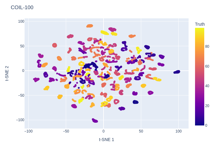
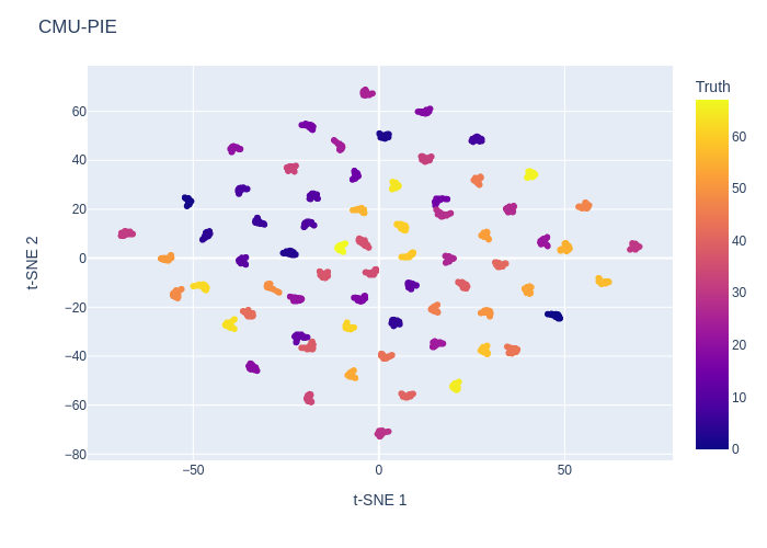
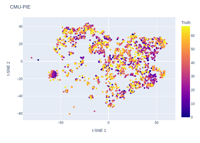
In both tasks, we analyze the rank correlation between retained spaces after the multimodality test, considering various indices (Figures 3 to 33). The observed grouping behavior varies with validity measures, and the number of generated spaces influences clustering outcomes, underscoring the impact of these factors. Additionally, we employ t-SNE plots (Van der Maaten & Hinton,, 2008) to compare embedding spaces selected and excluded by ACE (Figures 4 to 34). Two representative examples respectively based on Silhouette score (cosine distance) with JULE and Calinski-Harabasz index with DEPICT, are presented in Figure 2. In these figures, selected spaces tend to exhibit more compact and well-separated clusters aligned with true labels, highlighting their superior clustering performance. Further details and discussions are available in Appendix A.6.4.

Determination of the number of clusters
In this experiment, we address the challenge of an unknown number of clusters, denoted as , in the clustering process across all datasets. Similar to the hyperparameter tuning experiment, we conduct a grid search to explore various values of and identify the optimal one. Specifically, running both JULE and DEPICT with evenly distributed values of covering the true , we compute internal measure scores from resulting pairs of embedded data and partitioning results. In Table 2, we find that, similar to hyperparameter tuning experiments, ACE scores consistently exhibit the highest average rank correlation, while raw scores yield the lowest correlation. Additionally, ACE and pooled scores, calculated by averaging over embedding spaces, achieve better correlation than paired scores across most scenarios. We also report the optimal number of clusters obtained by each approach in brackets, revealing that ACE and pooled scores contribute to the choice of . For instance, in DEPICT, ACE selects and for different indices for YTF with true , while paired scores suggest . Results for other indices and ACC comparison are reported in Appendix A.6.4, showing similar findings.
| USPS (10) | YTF (41) | FRGC (20) | MNIST-test (10) | CMU-PIE (68) | UMist (20) | COIL-20 (20) | COIL-100 (100) | Average | ||||||||||
| JULE: Calinski-Harabasz index | ||||||||||||||||||
| Raw score | 0.44 (5) | 0.56 (5) | 0.95 (50) | 0.89 (50) | -0.93 (10) | -0.83 (10) | 0.43 (5) | 0.51 (5) | -0.37 (10) | -0.24 (10) | -0.33 (5) | -0.24 (5) | 0.74 (15) | 0.64 (15) | 0.53 (80) | 0.47 (80) | 0.18 | 0.22 |
| Paired score | 0.65 (10) | 0.64 (10) | 0.1 (50) | 0.06 (50) | -0.93 (15) | -0.83 (15) | 0.64 (10) | 0.6 (10) | -0.03 (20) | -0.02 (20) | -0.13 (5) | -0.07 (5) | 0.76 (15) | 0.71 (15) | 0.74 (80) | 0.56 (80) | 0.22 | 0.21 |
| Pooled score | 0.65 (10) | 0.64 (10) | 0.9 (50) | 0.78 (50) | -0.87 (15) | -0.72 (15) | 0.64 (10) | 0.6 (10) | 0.9 (70) | 0.73 (70) | -0.14 (5) | -0.11 (5) | 0.74 (15) | 0.64 (15) | 0.72 (80) | 0.64 (80) | 0.44 | 0.40 |
| ACE | 0.65 (10) | 0.64 (10) | 0.93 (50) | 0.83 (50) | -0.72 (15) | -0.67 (15) | 0.64 (10) | 0.6 (10) | 0.88 (70) | 0.73 (70) | -0.14 (5) | -0.11 (5) | 0.74 (15) | 0.64 (15) | 0.79 (80) | 0.69 (80) | 0.47 | 0.42 |
| JULE: Davies-Bouldin index | ||||||||||||||||||
| Raw score | -0.27 (45) | -0.29 (45) | 0.92 (45) | 0.78 (45) | 0.87 (50) | 0.72 (50) | -0.46 (45) | -0.42 (45) | 0.72 (100) | 0.47 (100) | 0.19 (50) | 0.16 (50) | -0.88 (45) | -0.79 (45) | -0.92 (20) | -0.82 (20) | 0.02 | -0.02 |
| Paired score | 0.54 (15) | 0.38 (15) | 0.15 (50) | 0.17 (50) | 0.85 (45) | 0.67 (45) | 0.43 (10) | 0.29 (10) | 0.78 (100) | 0.56 (100) | -0.08 (45) | 0.02 (45) | -0.26 (40) | -0.14 (40) | -0.9 (20) | -0.78 (20) | 0.19 | 0.15 |
| Pooled score | 0.98 (15) | 0.91 (15) | 0.83 (50) | 0.67 (50) | 0.82 (40) | 0.61 (40) | 0.79 (10) | 0.6 (10) | 0.82 (90) | 0.64 (90) | -0.21 (45) | -0.02 (45) | -0.76 (50) | -0.57 (50) | -0.92 (20) | -0.82 (20) | 0.29 | 0.25 |
| ACE | 0.98 (15) | 0.91 (15) | 0.83 (50) | 0.67 (50) | 0.87 (40) | 0.72 (40) | 0.79 (10) | 0.6 (10) | 0.85 (90) | 0.69 (90) | -0.21 (45) | -0.02 (45) | -0.69 (50) | -0.57 (50) | -0.94 (20) | -0.82 (20) | 0.31 | 0.27 |
| JULE: Silhouette score (cosine distance) | ||||||||||||||||||
| Raw score | 0.69 (20) | 0.51 (20) | 1.0 (50) | 1.0 (50) | 0.67 (30) | 0.5 (30) | 0.07 (10) | 0.02 (10) | -0.28 (60) | -0.11 (60) | 0.13 (50) | 0.07 (50) | -0.52 (45) | -0.43 (45) | 0.42 (200) | 0.24 (200) | 0.27 | 0.23 |
| Paired score | 0.99 (10) | 0.96 (10) | 0.3 (50) | 0.22 (50) | 0.72 (25) | 0.61 (25) | 0.87 (10) | 0.69 (10) | 0.98 (70) | 0.91 (70) | -0.07 (45) | 0.07 (45) | 0.52 (25) | 0.36 (25) | 0.39 (200) | 0.2 (200) | 0.59 | 0.50 |
| Pooled score | 0.95 (10) | 0.87 (10) | 0.98 (50) | 0.94 (50) | 0.68 (45) | 0.56 (45) | 0.96 (10) | 0.87 (10) | 0.98 (70) | 0.91 (70) | -0.07 (45) | -0.02 (45) | 0.71 (20) | 0.57 (20) | 0.41 (200) | 0.24 (200) | 0.70 | 0.62 |
| ACE | 0.95 (10) | 0.87 (10) | 0.98 (50) | 0.94 (50) | 0.7 (45) | 0.61 (45) | 0.96 (10) | 0.87 (10) | 0.98 (70) | 0.91 (70) | -0.07 (45) | -0.02 (45) | 0.74 (20) | 0.5 (20) | 0.46 (180) | 0.33 (180) | 0.71 | 0.63 |
| JULE: Silhouette score (euclidean distance) | ||||||||||||||||||
| Raw score | 0.56 (10) | 0.47 (10) | 1.0 (50) | 1.0 (50) | -0.18 (10) | -0.17 (10) | 0.61 (30) | 0.47 (30) | 0.55 (60) | 0.38 (60) | 0.19 (50) | 0.16 (50) | -0.41 (30) | -0.36 (30) | 0.39 (200) | 0.2 (200) | 0.34 | 0.27 |
| Paired score | 0.85 (10) | 0.73 (10) | 0.33 (50) | 0.28 (50) | 0.72 (25) | 0.61 (25) | 0.88 (10) | 0.69 (10) | 0.96 (80) | 0.87 (80) | 0.07 (45) | 0.16 (45) | 0.55 (25) | 0.43 (25) | 0.44 (200) | 0.29 (200) | 0.60 | 0.51 |
| Pooled score | 0.95 (10) | 0.87 (10) | 0.97 (50) | 0.89 (50) | 0.68 (45) | 0.56 (45) | 0.95 (10) | 0.82 (10) | 0.98 (70) | 0.91 (70) | 0.14 (45) | 0.11 (45) | 0.76 (25) | 0.57 (25) | 0.47 (200) | 0.33 (200) | 0.74 | 0.63 |
| ACE | 0.95 (10) | 0.87 (10) | 0.98 (50) | 0.94 (50) | 0.78 (45) | 0.67 (45) | 0.95 (10) | 0.82 (10) | 0.98 (70) | 0.91 (70) | 0.14 (45) | 0.11 (45) | 0.71 (25) | 0.43 (25) | 0.47 (200) | 0.33 (200) | 0.74 | 0.64 |
| DEPICT: Calinski-Harabasz index | ||||||||||||||||||
| Raw score | 0.46 (5) | 0.6 (5) | -0.69 (5) | -0.56 (5) | -0.88 (10) | -0.78 (10) | 0.46 (5) | 0.6 (5) | -0.92 (10) | -0.82 (10) | -0.31 | -0.19 | ||||||
| Paired score | 0.46 (5) | 0.6 (5) | -0.99 (5) | -0.96 (5) | -0.85 (10) | -0.72 (10) | 0.44 (5) | 0.56 (5) | -0.92 (10) | -0.82 (10) | -0.37 | -0.27 | ||||||
| Pooled score | 0.46 (5) | 0.6 (5) | -0.98 (5) | -0.91 (5) | -0.85 (10) | -0.72 (10) | 0.46 (5) | 0.6 (5) | 0.44 (10) | 0.56 (10) | -0.09 | 0.03 | ||||||
| ACE | 0.46 (5) | 0.6 (5) | -0.66 (5) | -0.51 (5) | 0.77 (30) | 0.61 (30) | 0.46 (5) | 0.6 (5) | 0.92 (80) | 0.82 (80) | 0.39 | 0.42 | ||||||
| DEPICT: Davies-Bouldin index | ||||||||||||||||||
| Raw score | -0.39 (45) | -0.42 (45) | 0.99 (50) | 0.96 (50) | 0.68 (50) | 0.39 (50) | -0.22 (35) | -0.16 (35) | 0.92 (100) | 0.82 (100) | 0.40 | 0.32 | ||||||
| Paired score | 0.46 (5) | 0.6 (5) | -0.78 (5) | -0.64 (5) | -0.85 (10) | -0.72 (10) | 0.44 (5) | 0.56 (5) | -0.1 (10) | 0.02 (10) | -0.17 | -0.04 | ||||||
| Pooled score | 0.6 (15) | 0.51 (15) | 0.88 (50) | 0.73 (50) | -0.13 (20) | -0.17 (20) | 0.74 (10) | 0.64 (10) | 0.92 (100) | 0.82 (100) | 0.60 | 0.51 | ||||||
| ACE | 0.62 (10) | 0.6 (10) | 0.95 (50) | 0.87 (50) | 0.77 (35) | 0.67 (35) | 0.78 (10) | 0.69 (10) | 0.96 (70) | 0.91 (70) | 0.82 | 0.75 | ||||||
| DEPICT: Silhouette score (cosine distance) | ||||||||||||||||||
| Raw score | -0.13 (25) | -0.11 (25) | 1.0 (50) | 1.0 (50) | 0.97 (45) | 0.89 (45) | 0.71 (15) | 0.56 (15) | -0.43 (60) | -0.33 (60) | 0.42 | 0.40 | ||||||
| Paired score | 0.44 (5) | 0.56 (5) | -0.7 (5) | -0.6 (5) | -0.85 (10) | -0.72 (10) | 0.44 (5) | 0.56 (5) | 0.07 (10) | 0.11 (10) | -0.12 | -0.02 | ||||||
| Pooled score | 0.6 (15) | 0.51 (15) | 0.61 (40) | 0.47 (40) | 0.07 (25) | 0.06 (25) | 0.71 (10) | 0.64 (10) | 0.98 (80) | 0.91 (80) | 0.59 | 0.52 | ||||||
| ACE | 0.65 (15) | 0.64 (15) | 0.87 (40) | 0.78 (40) | 0.93 (35) | 0.83 (35) | 0.85 (10) | 0.78 (10) | 0.99 (80) | 0.96 (80) | 0.86 | 0.80 | ||||||
| DEPICT: Silhouette score (euclidean distance) | ||||||||||||||||||
| Raw score | -0.34 (25) | -0.29 (25) | 1.0 (50) | 1.0 (50) | 0.3 (50) | 0.11 (50) | 0.39 (10) | 0.33 (10) | -0.43 (10) | -0.33 (10) | 0.18 | 0.16 | ||||||
| Paired score | 0.44 (5) | 0.56 (5) | -0.61 (5) | -0.47 (5) | -0.85 (10) | -0.72 (10) | 0.44 (5) | 0.56 (5) | -0.12 (10) | -0.02 (10) | -0.14 | -0.02 | ||||||
| Pooled score | 0.6 (15) | 0.51 (15) | 0.98 (50) | 0.91 (50) | 0.07 (25) | 0.06 (25) | 0.73 (10) | 0.69 (10) | 0.99 (80) | 0.96 (80) | 0.67 | 0.63 | ||||||
| ACE | 0.46 (5) | 0.6 (5) | 0.94 (40) | 0.87 (40) | 0.02 (25) | 0.06 (25) | 0.85 (10) | 0.78 (10) | 0.98 (80) | 0.91 (80) | 0.65 | 0.64 | ||||||
Ablation studies
In our two experiments, we conducted ablation studies to gain insights into crucial aspects of our proposed approach (see Appendix A.6.5). Our findings emphasize the significant role of the Dip test in enhancing ACE’s performance in specific tasks, while its impact on the pooled score remains marginal. Exploring different family-wise error rates () for edge inclusion in link analysis revealed consistent performance for different , underscoring the robustness of ACE across varying . The comparison of including all edges further highlighted the importance of the testing procedure for edge inclusion, as it led to significantly lower correlations in specific cases. Additionally, our examination of an alternative density-based clustering method, DBSCAN (Ester et al.,, 1996), showcased comparable evaluation performance, but the simplicity of HDBSCAN made it the preferred choice for grouping in our approach. Lastly, the comparison between two link analysis algorithms (HITS (Kleinberg,, 1999) and PageRank) favored PageRank, indicating slightly better performance, particularly due to its consideration of both incoming and outgoing links simultaneously. Collectively, these findings deepen our understanding of the components influencing ACE’s performance, offering valuable insights for its effective application across various clustering tasks.
6 Discussion and Future Work
This paper addresses the challenges in evaluating deep clustering methods by introducing a theoretical framework that revisits traditional validation measures’ limitations. The contributions encompass formal justifications, highlighting the necessity of rethinking evaluation approaches in the deep clustering setting, along with proposing a strategy based on admissible embedding spaces. Extensive experiments demonstrate the framework’s effectiveness in scenarios such as hyperparameter tuning, cluster number selection, and checkpoint selection. Considering the complexity introduced in the deep clustering setting, the paper is primarily focused on providing a systematic guideline and insights for deep clustering evaluation. Different indices define clustering goodness in distinct ways, highlighting the need for a nuanced understanding of each metric, which we leave as future research. The ACE approach relies on the existence of admissible spaces, and challenges arise in scenarios with too few or even no admissible spaces. The proposed strategy, demonstrated to be effective with , can be adapted for scenarios with too few admissible spaces, as discussed in Appendix A.6.5. The challenging scenario of no admissible spaces is discussed in the checkpoint selection experiment (Appendix A.6.4), where despite no significant departure from unimodality, pooled scores outperform paired scores across all indices. This suggests that direct pooling could be a viable solution when is small or no retained space after the multimodality test. Additionally, practitioners are encouraged to leverage empirical knowledge and exploratory data visualization techniques when deciding which spaces to incorporate. The analysis in Appendix A.6.4 underscores that effective spaces typically show compact and well-separated clusters. Our future work will further delve into providing detailed insights for various metrics in deep clustering evaluation.
References
- Agresti, (2010) Agresti, Alan. 2010. Analysis of ordinal categorical data. Vol. 656. John Wiley & Sons.
- Beyer et al., (1999) Beyer, Kevin, Goldstein, Jonathan, Ramakrishnan, Raghu, & Shaft, Uri. 1999. When Is “Nearest Neighbor” Meaningful? Pages 217–235 of: Beeri, Catriel, & Buneman, Peter (eds), Database Theory — ICDT’99. Berlin, Heidelberg: Springer Berlin Heidelberg.
- Caliński & Harabasz, (1974) Caliński, Tadeusz, & Harabasz, Jerzy. 1974. A dendrite method for cluster analysis. Communications in Statistics-theory and Methods, 3(1), 1–27.
- Caron et al., (2018) Caron, Mathilde, Bojanowski, Piotr, Joulin, Armand, & Douze, Matthijs. 2018. Deep clustering for unsupervised learning of visual features. Pages 132–149 of: Proceedings of European Conference on Computer Vision.
- Davies & Bouldin, (1979) Davies, David L, & Bouldin, Donald W. 1979. A cluster separation measure. IEEE transactions on pattern analysis and machine intelligence, 224–227.
- Deng et al., (2009) Deng, Jia, Dong, Wei, Socher, Richard, Li, Li-Jia, Li, Kai, & Fei-Fei, Li. 2009. Imagenet: A large-scale hierarchical image database. Pages 248–255 of: IEEE Conference on Computer Vision and Pattern Recognition.
- Desgraupes, (2013) Desgraupes, Bernard. 2013. Clustering indices. University of Paris Ouest-Lab Modal’X, 1(1), 34.
- Ding et al., (2002) Ding, Chris, He, Xiaofeng, Husbands, Parry, Zha, Hongyuan, & Simon, Horst D. 2002. PageRank, HITS and a unified framework for link analysis. Pages 353–354 of: Proceedings of the 25th annual international ACM SIGIR conference on Research and development in information retrieval.
- Dunn, (1974) Dunn, Joseph C. 1974. Well-separated clusters and optimal fuzzy partitions. Journal of cybernetics, 4(1), 95–104.
- Ester et al., (1996) Ester, Martin, Kriegel, Hans-Peter, Sander, Jörg, Xu, Xiaowei, et al. 1996. A density-based algorithm for discovering clusters in large spatial databases with noise. Pages 226–231 of: kdd, vol. 96.
- Ghasedi Dizaji et al., (2017) Ghasedi Dizaji, Kamran, Herandi, Amirhossein, Deng, Cheng, Cai, Weidong, & Huang, Heng. 2017. Deep clustering via joint convolutional autoencoder embedding and relative entropy minimization. Pages 5736–5745 of: Proceedings of IEEE International Conference on Computer Vision.
- Graham & Allinson, (1998) Graham, Daniel B, & Allinson, Nigel M. 1998. Characterising virtual eigensignatures for general purpose face recognition. Pages 446–456 of: Face Recognition. Springer.
- Hadipour et al., (2022) Hadipour, Hamid, Liu, Chengyou, Davis, Rebecca, Cardona, Silvia T, & Hu, Pingzhao. 2022. Deep clustering of small molecules at large-scale via variational autoencoder embedding and K-means. BMC bioinformatics, 23(4), 1–22.
- Hagberg et al., (2008) Hagberg, Aric, Swart, Pieter, & S Chult, Daniel. 2008. Exploring network structure, dynamics, and function using NetworkX. Tech. rept. Los Alamos National Lab.(LANL), Los Alamos, NM (United States).
- Halkidi & Vazirgiannis, (2001) Halkidi, Maria, & Vazirgiannis, Michalis. 2001. Clustering validity assessment: Finding the optimal partitioning of a data set. Pages 187–194 of: Proceedings 2001 IEEE international conference on data mining. IEEE.
- Halkidi & Vazirgiannis, (2008) Halkidi, Maria, & Vazirgiannis, Michalis. 2008. A density-based cluster validity approach using multi-representatives. Pattern Recognition Letters, 29(6), 773–786.
- Hartigan & Hartigan, (1985) Hartigan, John A, & Hartigan, Pamela M. 1985. The dip test of unimodality. The annals of Statistics, 70–84.
- Hennig, (2023) Hennig, Christian. 2023. fpc: Flexible Procedures for Clustering. R package version 2.2-11.
- Holm, (1979) Holm, Sture. 1979. A simple sequentially rejective multiple test procedure. Scandinavian journal of statistics, 65–70.
- Huang et al., (2021a) Huang, Yufang, Liu, Yifan, Steel, Peter AD, Axsom, Kelly M, Lee, John R, Tummalapalli, Sri Lekha, Wang, Fei, Pathak, Jyotishman, Subramanian, Lakshminarayanan, & Zhang, Yiye. 2021a. Deep significance clustering: a novel approach for identifying risk-stratified and predictive patient subgroups. Journal of the American Medical Informatics Association, 28(12), 2641–2653.
- Huang et al., (2021b) Huang, Yufang, Axsom, Kelly M, Lee, John, Subramanian, Lakshminarayanan, & Zhang, Yiye. 2021b. DICE: Deep Significance Clustering for Outcome-Aware Stratification. arXiv preprint arXiv:2101.02344.
- Hubert & Levin, (1976) Hubert, Lawrence J, & Levin, Joel R. 1976. A general statistical framework for assessing categorical clustering in free recall. Psychological bulletin, 83(6), 1072.
- JAIN et al., (1999) JAIN, AK, MURTY, MN, & FLYNN, PJ. 1999. Data Clustering: A Review. ACM Computing Surveys, 31(3).
- Kendall, (1938) Kendall, Maurice G. 1938. A new measure of rank correlation. Biometrika, 30(1/2), 81–93.
- Kiefer, (1964) Kiefer, J. 1964. The Advanced Theory of Statistics, Volume 2,” Inference and Relationship.”.
- Kleinberg, (1999) Kleinberg, Jon M. 1999. Authoritative sources in a hyperlinked environment. Journal of the ACM (JACM), 46(5), 604–632.
- Knight, (1966) Knight, William R. 1966. A computer method for calculating Kendall’s tau with ungrouped data. Journal of the American Statistical Association, 61(314), 436–439.
- Langville & Meyer, (2005) Langville, Amy N, & Meyer, Carl D. 2005. A survey of eigenvector methods for web information retrieval. SIAM review, 47(1), 135–161.
- LeCun et al., (1998) LeCun, Yann, Bottou, Léon, Bengio, Yoshua, & Haffner, Patrick. 1998. Gradient-based learning applied to document recognition. Proceedings of the IEEE, 86(11), 2278–2324.
- Li et al., (2023) Li, Shenghao, Guo, Hui, Zhang, Simai, Li, Yizhou, & Li, Menglong. 2023. Attention-based deep clustering method for scRNA-seq cell type identification. PLOS Computational Biology, 19(11), e1011641.
- Liu et al., (2010) Liu, Yanchi, Li, Zhongmou, Xiong, Hui, Gao, Xuedong, & Wu, Junjie. 2010. Understanding of internal clustering validation measures. Pages 911–916 of: 2010 IEEE international conference on data mining. IEEE.
- Malika et al., (2014) Malika, Charrad, Ghazzali, Nadia, Boiteau, Veronique, & Niknafs, Azam. 2014. NbClust: an R package for determining the relevant number of clusters in a data Set. J. Stat. Softw, 61, 1–36.
- Masci et al., (2011) Masci, Jonathan, Meier, Ueli, Cireşan, Dan, & Schmidhuber, Jürgen. 2011. Stacked convolutional auto-encoders for hierarchical feature extraction. Pages 52–59 of: International Conference on Artificial Neural Networks.
- McInnes et al., (2017) McInnes, Leland, Healy, John, & Astels, Steve. 2017. hdbscan: Hierarchical density based clustering. The Journal of Open Source Software, 2(11), 205.
- Min et al., (2018) Min, Erxue, Guo, Xifeng, Liu, Qiang, Zhang, Gen, Cui, Jianjing, & Long, Jun. 2018. A survey of clustering with deep learning: From the perspective of network architecture. IEEE Access, 6, 39501–39514.
- Nene et al., (1996) Nene, Sameer A, Nayar, Shree K, Murase, Hiroshi, et al. 1996. Columbia object image library (coil-20).
- Neville et al., (2020) Neville, Zachariah, Brownstein, Naomi, Ackerman, Maya, & Adolfsson, Andreas. 2020. clusterability: Performs Tests for Cluster Tendency of a Data Set. R package version 0.1.1.0.
- Page et al., (1998) Page, Lawrence, Brin, Sergey, Motwani, Rajeev, & Winograd, Terry. 1998. The pagerank citation ranking: Bring order to the web. Tech. rept. Technical report, stanford University.
- Pedregosa et al., (2011) Pedregosa, F., Varoquaux, G., Gramfort, A., Michel, V., Thirion, B., Grisel, O., Blondel, M., Prettenhofer, P., Weiss, R., Dubourg, V., Vanderplas, J., Passos, A., Cournapeau, D., Brucher, M., Perrot, M., & Duchesnay, E. 2011. Scikit-learn: Machine Learning in Python. Journal of Machine Learning Research, 12, 2825–2830.
- Ronen et al., (2022) Ronen, Meitar, Finder, Shahaf E, & Freifeld, Oren. 2022. Deepdpm: Deep clustering with an unknown number of clusters. Pages 9861–9870 of: Proceedings of the IEEE/CVF Conference on Computer Vision and Pattern Recognition.
- Rousseeuw, (1987) Rousseeuw, Peter J. 1987. Silhouettes: a graphical aid to the interpretation and validation of cluster analysis. Journal of computational and applied mathematics, 20, 53–65.
- Sarle, (1983) Sarle, WS. 1983. SAS Technical report a-108, cubic clustering criterion, SAS Institute Inc. URL: https://support. sas. com/documentation/onlinedoc/v82/techreport_a108. pdf.
- Seabold & Perktold, (2010) Seabold, Skipper, & Perktold, Josef. 2010. statsmodels: Econometric and statistical modeling with python. In: 9th Python in Science Conference.
- Sim et al., (2002) Sim, Terence, Baker, Simon, & Bsat, Maan. 2002. The CMU pose, illumination, and expression (PIE) database. Pages 53–58 of: Proceedings of fifth IEEE international conference on automatic face gesture recognition. IEEE.
- Song et al., (2013) Song, Chunfeng, Liu, Feng, Huang, Yongzhen, Wang, Liang, & Tan, Tieniu. 2013. Auto-encoder based data clustering. Pages 117–124 of: Iberoamerican Congress on Pattern Recognition.
- Spearman, (1961) Spearman, Charles. 1961. The proof and measurement of association between two things.
- Van der Maaten & Hinton, (2008) Van der Maaten, Laurens, & Hinton, Geoffrey. 2008. Visualizing data using t-SNE. Journal of machine learning research, 9(11).
- Vincent et al., (2008) Vincent, Pascal, Larochelle, Hugo, Bengio, Yoshua, & Manzagol, Pierre-Antoine. 2008. Extracting and composing robust features with denoising autoencoders. Pages 1096–1103 of: Proceedings of the 25th international conference on Machine learning.
- Wang & Jiang, (2018) Wang, Jinghua, & Jiang, Jianmin. 2018. An Unsupervised Deep Learning Framework via Integrated Optimization of Representation Learning and GMM-Based Modeling. Pages 249–265 of: Asian Conference on Computer Vision. Springer.
- Wang et al., (2018) Wang, Yiqi, Shi, Zhan, Guo, Xifeng, Liu, Xinwang, Zhu, En, & Yin, Jianping. 2018. Deep embedding for determining the number of clusters. In: Proceedings of the AAAI Conference on Artificial Intelligence, vol. 32.
- Wang et al., (2021) Wang, Zeya, Ni, Yang, Jing, Baoyu, Wang, Deqing, Zhang, Hao, & Xing, Eric. 2021. DNB: A joint learning framework for deep Bayesian nonparametric clustering. IEEE Transactions on Neural Networks and Learning Systems, 33(12), 7610–7620.
- Wolf et al., (2011) Wolf, Lior, Hassner, Tal, & Maoz, Itay. 2011. Face recognition in unconstrained videos with matched background similarity. Pages 529–534 of: IEEE Conference on Computer Vision and Pattern Recognition.
- Yang et al., (2017) Yang, Bo, Fu, Xiao, Sidiropoulos, Nicholas D, & Hong, Mingyi. 2017. Towards k-means-friendly spaces: Simultaneous deep learning and clustering. Pages 3861–3870 of: international conference on machine learning.
- Yang et al., (2016) Yang, Jianwei, Parikh, Devi, & Batra, Dhruv. 2016. Joint unsupervised learning of deep representations and image clusters. Pages 5147–5156 of: IEEE Conference on Computer Vision and Pattern Recognition.
- Zwillinger & Kokoska, (1999) Zwillinger, Daniel, & Kokoska, Stephen. 1999. CRC standard probability and statistics tables and formulae. Crc Press.
Appendix A Appendix.
A.1 Deep Clustering Algorithm
Deep clustering encompasses the projection of high-dimensional data into a low-dimensional feature space using deep neural networks, followed by the partitioning of the embedded data within the feature space to generate cluster labels. The primary learning objective of most deep clustering methods typically involves minimizing a clustering loss through the generated embedded data. In this paper, we discuss two primary categories of deep clustering methods: autoencoder-based and clustering deep neural network (CDNN)-based approaches, as outlined in (Min et al.,, 2018). The key distinction between these classes lies in the integration of autoencoders.
The autoencoder, a widely utilized neural network structure, is employed extensively for tasks involving reconstruction and feature extraction. Consisting of an encoder and a decoder, each of which can be either a fully-connected neural network or a convolutional neural network, the autoencoder’s decoder architecture typically mirrors that of the encoder. The encoder compresses input data into an embedding space, while the decoder reconstructs the input data based on these embeddings. In methods utilizing autoencoders, cluster analysis is conducted using the embedded data from the encoder component (Song et al.,, 2013; Yang et al.,, 2017; Ghasedi Dizaji et al.,, 2017). Convolutional autoencoders, renowned for learning image representations by jointly minimizing both reconstruction loss and clustering loss, find frequent application in clustering tasks (Vincent et al.,, 2008; Masci et al.,, 2011; Ronen et al.,, 2022).
Another category of deep clustering methods has emerged, aiming to jointly learn image clusters and embeddings without incorporating an autoencoder (Yang et al.,, 2016; Ghasedi Dizaji et al.,, 2017; Caron et al.,, 2018; Wang et al.,, 2021). These methods demonstrate promising performance in recovering true labels. Within this category, some approaches either train or fine-tune data embeddings from autoencoders and estimate cluster structures using conventional clustering techniques like -means (Yang et al.,, 2017) and Gaussian mixture models (Wang & Jiang,, 2018). Others introduce an end-to-end clustering pipeline within a unified learning framework, enhancing model scalability by directly minimizing a clustering loss atop a network (Yang et al.,, 2016; Caron et al.,, 2018; Wang et al.,, 2021). CDNN-based methods, in particular, exclusively necessitate a clustering loss and involve an iterative procedure for jointly updating the network and estimating cluster labels. They can circumvent the need for a decoder, a requirement in autoencoder-based models, making CDNN-based methods more efficient. This efficiency enables their wider applicability to large-scale datasets (Caron et al.,, 2018).
In the following sections, we provide more details regarding the deep clustering algorithms evaluated in this paper: JULE (Yang et al.,, 2016), DEPICT (Ghasedi Dizaji et al.,, 2017) and DeepCluster (Caron et al.,, 2018).
A.1.1 JULE
JULE (Yang et al.,, 2016) stands out as a joint unsupervised learning approach that employs agglomerative clustering techniques to train its feature extractor, deviating from the conventional use of autoencoders. JULE formulates joint learning within a recurrent framework. Here, the merging operations of agglomerative clustering serve as a forward pass for creating cluster labels, while the representation learning of deep neural networks constitutes the backward pass. JULE introduces a unified weighted triplet loss, optimizing it end-to-end to concurrently estimate cluster labels and deep embeddings. In each epoch, JULE systematically merges two clusters, computing the loss for the backward pass. The proposed loss in JULE achieves a dual purpose: it reduces inner-cluster distances and simultaneously increases intra-cluster distances.
A.1.2 DEPICT
DEPICT (Ghasedi Dizaji et al.,, 2017) follows an autoencoder-based framework. The approach includes stacking a multinomial logistic regression function on a multilayer convolutional autoencoder. DEPICT introduces a novel clustering loss designed to efficiently map data into a discriminative embedding subspace and precisely predict cluster assignments. This loss is defined through relative entropy minimization, further regularized by a prior on the frequency of cluster assignments. DEPICT employs a joint learning framework to concurrently minimize both the clustering loss and the reconstruction loss.
A.1.3 DeepCluster
DeepCluster is an end-to-end approach that simultaneously updates network parameters and image clusters. This method employs -means on features extracted from large deep convolutional neural networks, such as AlexNet and VGG-16, to predict cluster assignments. Subsequently, it utilizes these cluster assignments as “pseudo-labels” to optimize the parameters of the convolutional neural networks. Successfully applied to extensive datasets like ImageNet (Deng et al.,, 2009), this method has exhibited promising performance in learning visual features (Caron et al.,, 2018).
A.2 Technical Proofs
A.2.1 Proof of Theorem 1
Proof.
By Lemma 1, the distance function is meaningless in high dimension since all the points has asymptotically the same distance to the query point. Thus, any distance-based clustering validity index will converge to . ∎
A.2.2 Proof of Theorem 2
Proof.
Since is a consistent score, we have .
(1) If by definition we have . Thus
as .
(2) If ,
i) Consider the case where , i.e., and are the same.
So does not converge to 1.
ii) Consider the case where , without loss of generality we assume . Then we have the following decomposition:
The first quantity represents the clustering difference on space , and the second quantity represents the space difference. If the clustering difference is larger than the space difference, we then have . Since and are distinguishable, by definition we have for some . So
In summary, happens only when . ∎
A.2.3 Proof of Theorem 3
Proof.
By definition we have
and
Thus,
since and .
For the special case where is consistent in both and . We have a.s. if and only if a.s.. Thus,
∎
A.2.4 Proof of Corollary 1
Proof.
To set up the rank among the clusterings, we need to do times of pairwise comparison.
For any , by definition we have
and . So for any fixed pair of (, we have
and thus
∎
A.3 External Validation Measure
Normalized Mutual Information
Normalized Mutual Information (NMI) is a widely adopted metric for gauging the similarity between two distinct cluster assignments, denoted by sets and . The NMI is computed using the formula:
| (1) |
Here, denotes the mutual information between and , and stands for the entropy function. The NMI ranges between 0 (indicating no mutual information) and 1 (reflecting perfect correlation). In the context of clustering performance evaluation, when provided with true partition labels denoted as and estimated partition labels denoted as , we can leverage as a reliable metric.
Clustering accuracy
Clustering accuracy (ACC) is defined as the proportion of correctly matched pairs resulting from the optimal alignment of true class labels and predicted cluster labels. The clustering accuracy of with respect to is expressed as:
| (2) |
where denotes the set of all permutations of partition indices. Like accuracy in classification, clustering ACC computes the ratio of correct predictions to total predictions. However, it differs from classification accuracy by utilizing the best one-to-one mappings between predicted class memberships and ground-truth ones.
A.4 Clustering validity indices
In this section, we provide additional details for the clustering indices mentioned in the paper, which include the Silhouette score(Rousseeuw,, 1987), Dunn index (Dunn,, 1974; Desgraupes,, 2013),cubic clustering criterion (CCC) (Sarle,, 1983), Cindex (CIND) (Hubert & Levin,, 1976; Desgraupes,, 2013), Calinski-Harabasz index (Caliński & Harabasz,, 1974; Desgraupes,, 2013), Davies-Bouldin index (DB) (Davies & Bouldin,, 1979; Desgraupes,, 2013), SDBW index (SDBW) (Halkidi & Vazirgiannis,, 2001; Desgraupes,, 2013), and CDbw index (CDbw) (Halkidi & Vazirgiannis,, 2008). The data in used for clustering and evaluation purposes is denoted as . Here, represents the index set for the -th cluster, and its size is denoted as .
Let represent the barycenter of the observations in cluster , and let denote the barycenter of all observations (Desgraupes,, 2013).
| (3) | ||||
A.4.1 Silhouette Score (Rousseeuw,, 1987)
Using a chosen distance function to calculate the distance between observations and (i.e., and ), let represent the mean distance between the -th observation and all other observations in the same cluster .
| (4) |
Let represents the smallest mean distance of the -th observation to all observations in any other cluster, where represents clusters other than .
| (5) |
Then, a silhouette value of the observation can be defined as:
| (6) |
The silhouette score is defined as the mean of the mean silhouette value of a cluster throughout all clusters.:
| (7) |
A.4.2 Dunn Index (Dunn,, 1974)
Let represent the minimal distance between points of different clusters, and denote the largest within-cluster distance. The distance between clusters and is defined as the distance between their closest points:
| (8) |
and corresponds to the smallest among these distances :
| (9) |
For each cluster , let denote the largest distance between two distinct points within the cluster:
| (10) |
and corresponds to the largest of these distances :
| (11) |
The Dunn index is defined as the quotient of and :
| (12) |
A.4.3 Davies-Bouldin index (Davies & Bouldin,, 1979)
Let denote the mean distance of the points belonging to cluster to their barycenter :
| (13) |
Let denote the distance between the barycenters and of clusters and .
| (14) |
For each cluster , is defined as:
| (15) |
The Davies-Bouldin index is the mean value of across all the clusters:
| (16) |
A.4.4 Calinski-Harabasz index (Caliński & Harabasz,, 1974)
The within-cluster dispersion is defined as the sum of squared distances between the observations and the barycenter of the cluster:
| (17) |
Then, the pooled within-cluster sum of squares (WGSS) is the sum of the within-cluster dispersions for all the clusters:
| (18) |
Define the between-group dispersion (BGSS) as the dispersion of the cluster centers with respect to the center of the entire dataset.
| (19) |
The Calinski-Harabasz index is defined as:
| (20) |
A.4.5 Cindex (Hubert & Levin,, 1976)
For cluster , let represent the total number of pairs of distinct points in the cluster. Also, let denote the total number of pairs of distinct points in the whole dataset.
Define as the sum of the distances between all pairs of points inside each cluster.
Define as the sum of the smallest distances between all pairs of points in the whole dataset. There are such pairs: one takes the sum of the smallest values.
Define as the sum of the largest distances between all pairs of points in the whole dataset. There are such pairs: one takes the sum of the largest values.
The index is defined as:
| (21) |
A.4.6 SDBW index (Halkidi & Vazirgiannis,, 2001)
Consider the vector of variances for each variable in the data set , which is defined as:
| (22) |
For the cluster , let its associated data be denoted by . Then, we have:
| (23) |
Let be the mean of the norms of the vectors divided by the norm of vector :
| (24) |
Define as the square root of the sum of the norms of the variance vectors divided by the number of clusters:
| (25) |
The density for a given point, with respect to two clusters and , is determined by the number of points in these two clusters whose distance to this point is less than . In geometric terms, this involves considering the ball with a radius of centered at the given point and counting the number of points belonging to located within this ball.
For each pair of clusters and , calculate the densities for the barycenters and of the clusters, as well as for their midpoint . Define the quotient as the ratio between the density at the midpoint and the larger density of the two barycenters:
| (26) |
Define the between-cluster density as the average of the quotients :
| (27) |
The SDbw index is defined as :
| (28) |
A.4.7 Cubic clustering criterion (Sarle,, 1983)
Let represent a one-hot encoding matrix for the clustering membership of the observations in the data set. Assuming is the centered data, we can express this as:
| (29) |
Define the total-sample sum-of-square and crossproducts (SSCP) matrix as:
| (30) |
Define the between-cluster SSCP matrix as:
| (31) |
Then the with-cluster SSCP matrix is defined as:
| (32) |
Then the observed for the clustering result can be expressed as:
| (33) |
Consider approximating the value of for a population uniformly distributed on a hyperbox. Assume that the edges of the hyperbox are aligned with the coordinate axes. Let be the edge length of the hyperbox along the -th dimension, and given a sample , is the square root of the -th eigenvalue of . Assume further that the ’s are in decreasing order. Let be the volume of the hyperbox. If the hyperbox is divided into (i.e., ) hypercubes with edge length , then the volume of the hyperbox equals the total volume of the hypercubes. represents the number of hypercubes along the -th dimension of the hyperbox. Let be the largest integer less than such that is not less than one. Hence, we have
| (34) | ||||
Then, we can derive the following small-sample approximation for the expected value of :
| (35) |
The CCC is computed as
| (36) |
A.4.8 CDbw index (Halkidi & Vazirgiannis,, 2008)
Consider as a partitioning of the data. Let be the set of representative points for cluster , capturing the geometry of the . A representative point of cluster is deemed the closest representative in to the representative of cluster , denoted as , if is the representative point of with the minimum distance from . The respective Closest Representative points () between and are defined as the set of mutual closest representatives of the two clusters. Let be the -th pair of respective closest representative points of clusters and .
The density between clusters and is defined as follows:
| (37) |
where denotes the Euclidean distance between the pair of points defined by , represents the cardinality of the set , and the term indicates the average standard deviation of the considered clusters. The cardinality denotes the average number of points in and that belong to the neighborhood of .
The inter-cluster density is defined to measure, for each cluster , the maximum density between and the other clusters in :
| (38) |
Cluster separation (Sep) is defined to measure the separation of clusters, considering the inter-cluster density in relation to the distance between clusters:
| (39) |
where .
Then the relative intra-cluster density w.r.t a shrinkage factor is defined as follows:
| (40) |
where
The cardinality of a point represents the proportion of points in cluster that belong to the neighborhood of a representative determined by a factor (i.e., the representatives of shrunk by ), where the neighborhood of a data point, , is defined to be a hypersphere centered at it with a radius equal to the average standard deviation of the considered clusters, stdev.
The compactness of a clustering in terms of density is defined as:
| (41) |
where represents the number of different values that the factor takes, determining the density at various areas within clusters.
Intra-density changes is defined to measure the changes of density within clusters:
| (42) |
Cohesion is defined to measure the density within clusters w.r.t. the density changes observed within them:
| (43) |
SC (Separation w.r.t. Compactness) is defined to evaluate the clusters’ separation (the density between clusters) w.r.t. their compactness (the density within the clusters:
| (44) |
Then the CDbw index is defined as:
| (45) |
A.5 Additional Algorithms Details
A.5.1 Dip statistics ((Hartigan & Hartigan,, 1985))
In our quality assessment of each , the initial step involves ensuring that the embedded data is clusterable. Various methods have been developed for testing clusterability, typically achieving this by identifying the presence of more than one mode in the data distribution. This can be accomplished through kernel density estimation or testing order statistics, intervals, or distribution functions. In this paper, we opt for a widely applied multimodality testing method known as the Dip test. This method refrains from assuming any specific form for the underlying data distribution, making it straightforward to implement. The Dip test is designed to estimate the discrepancy between the cumulative distribution function (CDF) of the data and the nearest multimodal function. For a given CDF , the Dip is defined as , where represents the class of unimodal CDFs. Considering the empirical CDF of the embedded data , the Dip of asymptotically converges to the Dip of (i.e., ). In the Dip test, a uniform distribution is chosen as a“null” model. Hartigan and Hartigan (Hartigan & Hartigan,, 1985) conjectured that is the “asymptotically least favorable” unimodal distribution—essentially, the most challenging to distinguish from multimodal distributions as increases. The Dip of the empirical CDF can be obtained through an algorithm. For detailed implementation, please refer to Appendix A.5.1. Following that, p-values for the Dip test under the null hypothesis that is a unimodal distribution are derive through Monte Carlo simulations with . From these computed p-values from different , with a multiple testing procedure (specifically, the Holm–Bonferroni method with family-wise error rate (FWER) of applied in this paper (Holm,, 1979)), we will select only those embedding spaces that reject the null hypothesis, indicating that is not unimodal.
The Dip statistic, denoted as , for the empirical cumulative distribution function (CDF) can be computed using the analogy of stretching a taut string. Further details of the algorithm can be found below:
-
1.
Set: , , .
-
2.
Calculate the greatest convex minorant and least concave majorant for in ; suppose the points of contact with are respectively and .
-
3.
Suppose and that the supreme occurs at . Define , .
-
4.
Suppose and that the supreme occurs at . Define , .
-
5.
If , stop and set .
-
6.
If , set .
-
7.
Set , and return to step 2.
A.5.2 Stage-wise clustering
The details of the stage-wise clustering algorithm can be seen in Algorithm 2.
-
1.
For each , define the distance
-
2.
Run density-based clustering method based on
-
3.
Return groups of spaces (each ) excluding outlier spaces
-
1.
For each group , apply density-based clustering on
-
2.
For each group , generate subgroups and outlier spaces
-
3.
Treat each outlier space as a singleton subgroup. Incorporate these singleton subgroups with all the subgroups created for all groups to obtain mutually exclusive subgroups
Note that in Algorithm 2, we omit outlier spaces from density-based clustering in the first phase, treating them as rank uncorrelated spaces. In the second phase, we handle and incorporate outlier spaces as singleton subgroups. The distinction lies in the fact that the second phase is solely intended for grouping spaces with similar score magnitudes, while the first phase is employed to identify rank-correlated spaces. Further details on the decision to include or exclude outlier spaces in Phase 1 can be found in Appendix A.6.5.
A.5.3 Link analysis
Given a graph or network, link analysis is a valuable technique for assessing relationships between nodes and assigning importance to each node. Two prominent algorithms commonly employed for link analysis are:
Hyperlink-Induced Topic Search (HITS) algorithm
The HITS algorithm is based on an intuition that a good authority node is linked to by numerous quality hub nodes, and a good hub node links to numerous trusted authorities. For each node , HITS computes an value based on incoming links and a value based on outgoing links. This mutually reinforcing relationship is mathematically expressed through the following operations:
| (46) |
PageRank (PR) algorithm
The PageRank (PR) algorithm shares a similar idea with HITS that a good node should be connected to or pointed to by other good nodes. PR adopts a web surfing model based on a Markov process, introducing a different approach for determine the scores compared to the mutual reinforcement concept in HITS.
Let be a stochastic matrix, obtained by rescaling the adjacency matrix such that each row sums to one. Here, represents the probability of transitioning from node to . Incorporating the idea of link-interrupting jumps, the matrix is adjusted by adding a matrix consisting of all ones, resulting in , where . Then the authority score in PR, indicating each node’s importance, is determined by the equilibrium distribution , satisfying through the equation:
| (47) |
A.6 Additional Experimental Details
The data information for the datasets COIL20 (Nene et al.,, 1996), COIL100 (Nene et al.,, 1996), CMU-PIE (Sim et al.,, 2002), YTF (Wolf et al.,, 2011), USPS 444https://cs.nyu.edu/~roweis/data.html, MNIST-test (LeCun et al.,, 1998), UMist (Graham & Allinson,, 1998), FRGC 555http://www3.nd.edu/~cvrl/CVRL/Data$_$Sets.html is provided in Table 3.
A.6.1 Data information
| Dataset | #Samples | Image Size | #Classes |
|---|---|---|---|
| COIL20 | 1440 | 128128 | 20 |
| COIL100 | 7200 | 128128 | 100 |
| CMU-PIE | 2856 | 3232 | 68 |
| YTF | 1 | 5555 | 41 |
| USPS | 11000 | 1616 | 10 |
| MNIST-test | 1 | 2828 | 10 |
| UMist | 575 | 11292 | 20 |
| FRGC | 2462 | 3232 | 20 |
A.6.2 Evaluation metrics
Spearman’s rank correlation coefficient (Spearman,, 1961; Zwillinger & Kokoska,, 1999; Kiefer,, 1964)
Spearman’s rank correlation coefficient, denoted as , is a nonparametric measure of rank correlation that assesses the strength and direction of monotonic relationships between two variables. It is calculated by considering the Pearson correlation, denoted as , between the ranks of the variables and has a range between and .
Given raw scores of two variables and , the scores are initially converted into their respective ranks, denoted as and . With these ranks, is then computed as:
| (48) |
where is the covariance of the rank variables. and are the standard deviations of the rank variables.
The test for Spearman’s rho tests the following null hypothesis (): , which corresponds to no monotonic relationship between the two variables in the population. The alternative hypothesis () can be two-sided: , right-sided: , and left-sided: . The test statistic is given by:
| (49) |
which follows an approximate distribution as Student’s t-distribution under the null hypothesis.
Kendall rank correlation coefficient (Kendall,, 1938; Agresti,, 2010; Knight,, 1966)
The Kendall rank correlation coefficient () serves as a statistical metric quantifying the ordinal association between two measured quantities. As a measure of rank correlation, it ranges from (indicating perfect inversion) to (representing perfect agreement), with a value of zero signifying an absence of association. A higher between two variables suggests that observations share similar ranks across both variables, while a lower correlation indicates dissimilar ranks between the observations in the two variables.
Consider the set of observations for the joint random variables and . For any pair of observations and , where , they are deemed concordant if the sort order of and aligns. In other words, if either both and or both and holds, the observations are concordant. When either or , and form a tied pair; when a pair is neither concordant nor tied, they are discordant.
The Kendall coefficient is defined as:
| (50) |
where , , . represents the count of concordant pairs, while indicates the count of discordant pairs. Moreover, denotes the number of tied values in the -th group of ties for the first quantity (e.g., for the pair ), and signifies the number of tied values in the -th group of ties for the second quantity (e.g., for the pair ). The count of discordant pairs is equivalent to the inversion number, representing the count of rearrangements needed to permute the -sequence with the order of the -sequence.
A.6.3 Additional implementation details
In this section, we provide additional details regarding our experiments. The deep clustering models, JULE, DEPICT, and DeepCluster, are executed using the source code from the respective original papers. For computing clustering validity indices such as Silhouette score (Rousseeuw,, 1987), Calinski-Harabasz index, and Davies-Bouldin index (Davies & Bouldin,, 1979), we utilize functions from the sklearn (Pedregosa et al.,, 2011) library in Python. The computation of Cubic clustering criterion (CCC) (Sarle,, 1983), Dunn index (Dunn,, 1974), Cindex (Hubert & Levin,, 1976), SDbw index (Halkidi & Vazirgiannis,, 2001) involves using R and follows the implementation detailed in (Malika et al.,, 2014). For CDbw index (Halkidi & Vazirgiannis,, 2008), we calculate scores using the function provided by the R package fpc (Hennig,, 2023). The Dip test is implemented in R using the function from the R package clusterability (Neville et al.,, 2020). By default, the package conducts a PCA dimension reduction on the tested data before performing the test. The link analysis algorithms are implemented using the Python library networkx (Hagberg et al.,, 2008). All other statistical tests are implemented using the Python library statsmodels (Seabold & Perktold,, 2010). The HDBSCAN clustering is implemented using the Python library hdbscan (McInnes et al.,, 2017), and DBSCAN is implemented using sklearn. The entire implementation of ACE is carried out in Python.
Hyperparameter tuning
For the JULE algorithm, we construct the search space by selecting the learning rate from the list and the unfolding rate () from the list , resulting in hyperparameter combinations. For the DEPICT algorithm, we define the search space by choosing the learning rate from the list and the balancing parameter of the reconstruction loss function from the list , yielding hyperparameter combinations. For each combination, we execute the two algorithms, and if a training trial fails, we consider the clustering results as missing and exclude that specific combination from the final evaluation.
Determination of the number of clusters
In this experimental setup, when running JULE and DEPICT across datasets, we search for among ten different values that are evenly distributed, covering the true . To create the search space for , we specify the following intervals: for the datasets FRGC, MNIST-test, USPS, UMist, YTF, and COIL-20, we use ; for CMU-PIE, we choose ; and for COIL-100, we apply . Here, denotes the generation of evenly spaced numbers over the specified interval with a total of values. For each , we run the clustering algorithm, and in the event of a training trial failure, we consider the clustering results as missing, excluding that specific from the final evaluation.
Selection of checkpoints
In consideration of training time and computational resources, we choose to download the validation set from ImageNet (Deng et al.,, 2009) rather than the training set, which consists of approximately images uniformly distributed across classes. To expedite training, we initialize the network by loading pre-trained weights from DeepCluster, which were obtained through training on 1.3 million images from the ImageNet training set. We adhere to the training settings specified in the source code, making adjustments only to the maximum number of clusters, set to . The deep clustering process runs for epochs, with checkpoints saved every five epochs, resulting in a total of checkpoints. At each checkpoint, we input the data to generate -dimensional features used for clustering and the corresponding estimated cluster assignments for evaluation.
A.6.4 Additional results
Hyperparameter tuning - NMI
In this section, we delve into additional results for the hyperparameter tuning task, with a specific focus on the rank correlation between measure scores and Normalized Mutual Information (NMI). The evaluated validity indices, including Cubic Clustering Criterion (CCC), Dunn index, Cindex, SDbw index, and CDbw index, are presented in Table 4. Both ACE and pooled scores demonstrate superior rank correlation with NMI in comparison to paired scores, showcasing their effectiveness over raw scores. It’s important to highlight the practical challenges of obtaining raw scores due to the high dimensional input data, as indicated by the dash mark. Furthermore, in certain cases, all four scores exhibit negative rank correlation with NMI, indicating the absence of admissible spaces for this metric in the dataset. Additionally, for JULE, the density-based validity index CDbw shows a noteworthy negative correlation of NMI with paired scores, pooled scores, and ACE scores across several datasets. However, it achieves high correlation on datasets UMist, COIL-20, and COIL-100, which displays non-convex shaped clusters in the output embedding spaces (suggested by Figures 4 to 6)). This observation suggests that density-based validity indices can offer more accurate evaluations for non-convex shape clustering results.
| USPS | YTF | FRGC | MNIST-test | CMU-PIE | UMist | COIL-20 | COIL-100 | Average | ||||||||||
| JULE: Cubic clustering criterion | ||||||||||||||||||
| Raw score | - | - | - | - | - | - | - | - | - | - | - | - | - | - | - | - | - | - |
| Paired score | 0.17 | 0.13 | 0.62 | 0.49 | 0.61 | 0.45 | 0.46 | 0.33 | 0.82 | 0.66 | 0.71 | 0.51 | 0.74 | 0.57 | 0.68 | 0.51 | 0.60 | 0.46 |
| Pooled score | 0.84 | 0.68 | 0.92 | 0.80 | 0.30 | 0.22 | 0.82 | 0.67 | 0.94 | 0.82 | 0.80 | 0.59 | 0.61 | 0.46 | 0.89 | 0.73 | 0.77 | 0.62 |
| ACE | 0.87 | 0.72 | 0.93 | 0.83 | 0.23 | 0.15 | 0.82 | 0.65 | 0.98 | 0.91 | 0.84 | 0.64 | 0.93 | 0.78 | 0.93 | 0.80 | 0.82 | 0.69 |
| JULE: Dunn index | ||||||||||||||||||
| Raw score | 0.12 | 0.10 | 0.56 | 0.43 | -0.07 | -0.04 | -0.17 | -0.13 | -0.37 | -0.21 | - | - | 0.54 | 0.44 | 0.71 | 0.52 | 0.19 | 0.16 |
| Paired score | -0.23 | -0.16 | 0.59 | 0.42 | 0.42 | 0.29 | -0.23 | -0.14 | 0.90 | 0.74 | 0.37 | 0.28 | 0.58 | 0.43 | 0.37 | 0.25 | 0.35 | 0.26 |
| Pooled score | -0.12 | -0.04 | 0.71 | 0.53 | 0.50 | 0.34 | -0.42 | -0.30 | 0.89 | 0.76 | 0.63 | 0.48 | 0.73 | 0.54 | 0.85 | 0.67 | 0.47 | 0.37 |
| ACE | -0.57 | -0.39 | 0.63 | 0.47 | 0.27 | 0.19 | -0.13 | -0.09 | 0.93 | 0.82 | 0.61 | 0.47 | 0.74 | 0.54 | 0.80 | 0.59 | 0.41 | 0.33 |
| JULE: Cindex | ||||||||||||||||||
| Raw score | 0.49 | 0.37 | 0.27 | 0.20 | -0.46 | -0.31 | 0.17 | 0.14 | -0.81 | -0.68 | - | - | 0.50 | 0.36 | 0.80 | 0.62 | 0.14 | 0.10 |
| Paired score | 0.27 | 0.19 | 0.09 | 0.06 | -0.28 | -0.19 | 0.47 | 0.33 | -0.49 | -0.35 | 0.53 | 0.37 | 0.06 | 0.04 | -0.17 | -0.09 | 0.06 | 0.05 |
| Pooled score | 0.65 | 0.45 | 0.67 | 0.52 | 0.02 | 0.02 | 0.73 | 0.57 | -0.11 | -0.08 | 0.58 | 0.42 | 0.51 | 0.37 | 0.76 | 0.57 | 0.48 | 0.36 |
| ACE | 0.78 | 0.62 | 0.20 | 0.13 | -0.16 | -0.11 | 0.83 | 0.67 | -0.55 | -0.35 | 0.58 | 0.42 | 0.77 | 0.58 | 0.69 | 0.52 | 0.39 | 0.31 |
| JULE: SDbw index | ||||||||||||||||||
| Raw score | -0.44 | -0.26 | - | - | -0.18 | -0.11 | -0.76 | -0.58 | -0.99 | -0.92 | - | - | -0.17 | -0.07 | - | - | -0.51 | -0.39 |
| Paired score | -0.16 | -0.08 | -0.54 | -0.38 | -0.12 | -0.08 | -0.44 | -0.30 | -0.25 | -0.16 | 0.69 | 0.48 | 0.52 | 0.37 | 0.24 | 0.22 | -0.01 | 0.01 |
| Pooled score | -0.38 | -0.24 | -0.62 | -0.45 | 0.18 | 0.12 | -0.56 | -0.40 | -0.76 | -0.65 | 0.24 | 0.17 | 0.10 | 0.13 | 0.61 | 0.41 | -0.15 | -0.11 |
| ACE | -0.35 | -0.18 | -0.64 | -0.45 | 0.47 | 0.36 | -0.18 | -0.11 | -0.52 | -0.52 | 0.64 | 0.46 | 0.61 | 0.45 | 0.74 | 0.54 | 0.10 | 0.07 |
| JULE: CDbw index | ||||||||||||||||||
| Raw score | -0.26 | -0.21 | - | - | - | - | - | - | -0.27 | -0.22 | - | - | - | - | - | - | -0.26 | -0.21 |
| Paired score | -0.24 | -0.16 | -0.23 | -0.17 | -0.38 | -0.27 | -0.60 | -0.43 | -0.07 | -0.05 | 0.07 | 0.06 | 0.33 | 0.21 | 0.50 | 0.35 | -0.08 | -0.06 |
| Pooled score | -0.38 | -0.25 | -0.55 | -0.40 | 0.26 | 0.17 | -0.73 | -0.54 | 0.71 | 0.63 | 0.73 | 0.52 | 0.85 | 0.68 | 0.90 | 0.72 | 0.22 | 0.19 |
| ACE | -0.31 | -0.20 | -0.58 | -0.41 | 0.31 | 0.21 | -0.70 | -0.52 | 0.62 | 0.52 | 0.75 | 0.55 | 0.80 | 0.61 | 0.97 | 0.85 | 0.23 | 0.20 |
| DEPICT: Cubic clustering criterion | ||||||||||||||||||
| Raw score | - | - | - | - | - | - | - | - | - | - | - | - | ||||||
| Paired score | 0.74 | 0.52 | 0.50 | 0.35 | 0.95 | 0.83 | 0.89 | 0.71 | 0.89 | 0.70 | 0.79 | 0.62 | ||||||
| Pooled score | 0.96 | 0.83 | 0.61 | 0.48 | 0.92 | 0.82 | 0.98 | 0.90 | 0.95 | 0.84 | 0.88 | 0.77 | ||||||
| ACE | 0.96 | 0.84 | 0.76 | 0.62 | 0.95 | 0.83 | 0.96 | 0.87 | 0.95 | 0.84 | 0.91 | 0.80 | ||||||
| DEPICT: Dunn index | ||||||||||||||||||
| Raw score | 0.56 | 0.41 | 0.42 | 0.26 | 0.59 | 0.47 | 0.88 | 0.73 | 0.15 | 0.05 | 0.52 | 0.39 | ||||||
| Paired score | 0.85 | 0.66 | 0.55 | 0.41 | 0.81 | 0.62 | 0.91 | 0.78 | 0.39 | 0.29 | 0.70 | 0.55 | ||||||
| Pooled score | 0.85 | 0.67 | 0.75 | 0.59 | 0.82 | 0.62 | 0.91 | 0.74 | 0.81 | 0.65 | 0.83 | 0.66 | ||||||
| ACE | 0.92 | 0.78 | 0.68 | 0.53 | 0.65 | 0.50 | 0.84 | 0.67 | 0.94 | 0.80 | 0.80 | 0.66 | ||||||
| DEPICT: Cindex | ||||||||||||||||||
| Raw score | -0.27 | -0.19 | -0.35 | -0.27 | 0.52 | 0.41 | 0.09 | 0.06 | -0.23 | -0.28 | -0.05 | -0.05 | ||||||
| Paired score | 0.53 | 0.36 | -0.03 | -0.02 | 0.24 | 0.19 | 0.44 | 0.35 | -0.18 | 0.01 | 0.20 | 0.18 | ||||||
| Pooled score | 0.70 | 0.54 | 0.53 | 0.40 | 0.88 | 0.74 | 0.92 | 0.80 | 0.53 | 0.37 | 0.71 | 0.57 | ||||||
| ACE | 0.90 | 0.75 | 0.61 | 0.45 | 0.91 | 0.77 | -0.39 | -0.27 | 0.73 | 0.57 | 0.55 | 0.45 | ||||||
| DEPICT: SDbw index | ||||||||||||||||||
| Raw score | 0.18 | 0.09 | - | - | 0.57 | 0.43 | 0.14 | 0.09 | -0.94 | -0.80 | -0.01 | -0.05 | ||||||
| Paired score | 0.84 | 0.67 | 0.55 | 0.36 | 0.91 | 0.77 | 0.89 | 0.74 | 0.57 | 0.46 | 0.75 | 0.60 | ||||||
| Pooled score | 0.93 | 0.79 | 0.62 | 0.48 | 0.75 | 0.61 | 0.96 | 0.87 | 0.67 | 0.49 | 0.79 | 0.65 | ||||||
| ACE | 0.93 | 0.79 | 0.64 | 0.48 | 0.89 | 0.75 | 0.97 | 0.90 | 0.95 | 0.84 | 0.87 | 0.75 | ||||||
| DEPICT: CDbw index | ||||||||||||||||||
| Raw score | - | - | - | - | - | - | - | - | 0.18 | 0.14 | 0.18 | 0.14 | ||||||
| Paired score | 0.48 | 0.35 | 0.61 | 0.40 | 0.83 | 0.66 | 0.63 | 0.46 | 0.88 | 0.70 | 0.69 | 0.51 | ||||||
| Pooled score | 0.95 | 0.86 | 0.64 | 0.48 | 0.78 | 0.63 | 0.50 | 0.32 | 0.92 | 0.79 | 0.76 | 0.62 | ||||||
| ACE | 0.69 | 0.53 | 0.64 | 0.48 | 0.81 | 0.66 | 0.50 | 0.32 | 0.94 | 0.83 | 0.72 | 0.56 | ||||||
Hyperparameter tuning - ACC
In this section, we present the rank correlation between different scores and clustering accuracy (ACC) across all validity indices, detailed in Table 5 and Table 6. The findings are consistent with our observations in Tables 1 and 4, which assess performance using NMI, thereby reinforcing our conclusions regarding the evaluation of deep clustering using these four scores.
| USPS | YTF | FRGC | MNIST-test | CMU-PIE | UMist | COIL-20 | COIL-100 | Average | ||||||||||
| JULE: Davies-Bouldin index | ||||||||||||||||||
| Raw score | -0.67 | -0.43 | -0.45 | -0.30 | -0.04 | -0.01 | -0.94 | -0.80 | -0.96 | -0.86 | -0.77 | -0.60 | -0.56 | -0.38 | -0.83 | -0.64 | -0.65 | -0.50 |
| Paired score | -0.27 | -0.15 | -0.14 | -0.09 | -0.23 | -0.14 | -0.35 | -0.19 | 0.20 | 0.16 | 0.53 | 0.36 | 0.63 | 0.44 | 0.33 | 0.26 | 0.09 | 0.08 |
| Pooled score | -0.49 | -0.20 | -0.35 | -0.23 | 0.48 | 0.36 | -0.35 | -0.21 | 0.89 | 0.75 | 0.17 | 0.11 | -0.29 | -0.22 | -0.48 | -0.34 | -0.05 | 0.00 |
| ACE | -0.30 | -0.09 | -0.07 | -0.07 | 0.53 | 0.38 | 0.79 | 0.64 | 0.07 | 0.03 | 0.27 | 0.20 | 0.21 | 0.18 | 0.44 | 0.28 | 0.24 | 0.19 |
| JULE: Calinski-Harabasz index | ||||||||||||||||||
| Raw score | 0.70 | 0.59 | 0.54 | 0.39 | -0.52 | -0.35 | 0.91 | 0.76 | -0.98 | -0.91 | -0.50 | -0.35 | -0.29 | -0.17 | 0.36 | 0.23 | 0.03 | 0.02 |
| Paired score | 0.04 | 0.05 | 0.39 | 0.27 | -0.26 | -0.18 | 0.31 | 0.21 | -0.20 | -0.12 | 0.64 | 0.45 | 0.57 | 0.40 | 0.09 | 0.08 | 0.20 | 0.14 |
| Pooled score | 0.91 | 0.78 | 0.78 | 0.61 | 0.30 | 0.21 | 0.91 | 0.77 | 0.95 | 0.83 | 0.81 | 0.60 | 0.58 | 0.43 | 0.90 | 0.75 | 0.77 | 0.62 |
| ACE | 0.90 | 0.77 | 0.73 | 0.54 | 0.49 | 0.36 | 0.95 | 0.82 | 0.97 | 0.87 | 0.81 | 0.61 | 0.57 | 0.40 | 0.93 | 0.81 | 0.79 | 0.65 |
| JULE: Silhouette score (cosine distance) | ||||||||||||||||||
| Raw score | 0.77 | 0.59 | 0.64 | 0.47 | 0.31 | 0.21 | 0.79 | 0.61 | 0.69 | 0.54 | -0.37 | -0.27 | -0.16 | -0.13 | 0.06 | 0.02 | 0.34 | 0.26 |
| Paired score | 0.17 | 0.14 | 0.59 | 0.41 | 0.07 | 0.06 | 0.47 | 0.33 | 0.45 | 0.33 | 0.64 | 0.46 | 0.70 | 0.51 | 0.64 | 0.45 | 0.47 | 0.34 |
| Pooled score | 0.74 | 0.68 | 0.73 | 0.55 | 0.71 | 0.53 | 0.90 | 0.73 | 0.96 | 0.88 | 0.75 | 0.55 | 0.20 | 0.11 | 0.61 | 0.44 | 0.70 | 0.56 |
| ACE | 0.96 | 0.85 | 0.74 | 0.55 | 0.82 | 0.65 | 0.92 | 0.78 | 0.98 | 0.92 | 0.78 | 0.58 | 0.41 | 0.32 | 0.84 | 0.68 | 0.81 | 0.67 |
| JULE: Silhouette score (euclidean distance) | ||||||||||||||||||
| Raw score | 0.92 | 0.77 | 0.59 | 0.43 | 0.27 | 0.19 | 0.83 | 0.66 | 0.35 | 0.32 | -0.35 | -0.24 | -0.14 | -0.05 | 0.14 | 0.08 | 0.33 | 0.27 |
| Paired score | 0.14 | 0.12 | 0.54 | 0.39 | -0.08 | -0.02 | 0.41 | 0.27 | 0.36 | 0.27 | 0.64 | 0.46 | 0.67 | 0.48 | 0.44 | 0.31 | 0.39 | 0.28 |
| Pooled score | 0.73 | 0.67 | 0.66 | 0.49 | 0.70 | 0.53 | 0.89 | 0.72 | 0.97 | 0.88 | 0.77 | 0.57 | 0.20 | 0.11 | 0.62 | 0.45 | 0.69 | 0.55 |
| ACE | 0.93 | 0.78 | 0.63 | 0.48 | 0.71 | 0.53 | 0.92 | 0.78 | 0.98 | 0.91 | 0.86 | 0.68 | 0.39 | 0.30 | 0.84 | 0.68 | 0.78 | 0.64 |
| JULE: Cubic clustering criterion | ||||||||||||||||||
| Raw score | - | - | - | - | - | - | - | - | - | - | - | - | - | - | - | - | - | - |
| Paired score | 0.04 | 0.05 | 0.43 | 0.30 | 0.52 | 0.35 | 0.30 | 0.20 | 0.84 | 0.67 | 0.65 | 0.48 | 0.76 | 0.58 | 0.67 | 0.49 | 0.53 | 0.39 |
| Pooled score | 0.91 | 0.78 | 0.76 | 0.59 | 0.33 | 0.23 | 0.91 | 0.77 | 0.95 | 0.84 | 0.80 | 0.59 | 0.57 | 0.42 | 0.90 | 0.76 | 0.77 | 0.62 |
| ACE | 0.94 | 0.82 | 0.76 | 0.59 | 0.21 | 0.14 | 0.88 | 0.72 | 0.99 | 0.93 | 0.84 | 0.65 | 0.91 | 0.74 | 0.93 | 0.79 | 0.81 | 0.67 |
| JULE: Dunn index | ||||||||||||||||||
| Raw score | 0.02 | 0.02 | 0.21 | 0.17 | -0.18 | -0.13 | -0.09 | -0.08 | -0.33 | -0.20 | - | - | 0.50 | 0.40 | 0.62 | 0.44 | 0.11 | 0.09 |
| Paired score | -0.36 | -0.24 | 0.29 | 0.19 | 0.55 | 0.39 | -0.20 | -0.14 | 0.89 | 0.73 | 0.31 | 0.24 | 0.56 | 0.42 | 0.40 | 0.28 | 0.31 | 0.23 |
| Pooled score | -0.35 | -0.16 | 0.35 | 0.23 | 0.62 | 0.44 | -0.52 | -0.37 | 0.87 | 0.72 | 0.59 | 0.45 | 0.72 | 0.53 | 0.73 | 0.54 | 0.38 | 0.30 |
| ACE | -0.77 | -0.56 | 0.38 | 0.25 | 0.46 | 0.33 | -0.10 | -0.09 | 0.92 | 0.79 | 0.58 | 0.44 | 0.73 | 0.54 | 0.67 | 0.49 | 0.36 | 0.27 |
| JULE: Cindex | ||||||||||||||||||
| Raw score | 0.56 | 0.45 | 0.35 | 0.24 | -0.52 | -0.37 | 0.24 | 0.23 | -0.80 | -0.67 | - | - | 0.56 | 0.40 | 0.78 | 0.61 | 0.17 | 0.13 |
| Paired score | 0.13 | 0.10 | -0.09 | -0.06 | -0.47 | -0.32 | 0.33 | 0.21 | -0.56 | -0.40 | 0.54 | 0.38 | 0.09 | 0.06 | -0.21 | -0.14 | -0.03 | -0.02 |
| Pooled score | 0.82 | 0.63 | 0.62 | 0.45 | -0.24 | -0.16 | 0.87 | 0.67 | -0.06 | -0.05 | 0.67 | 0.51 | 0.60 | 0.45 | 0.77 | 0.59 | 0.51 | 0.38 |
| ACE | 0.85 | 0.70 | 0.17 | 0.13 | -0.39 | -0.28 | 0.93 | 0.76 | -0.52 | -0.32 | 0.67 | 0.50 | 0.81 | 0.63 | 0.68 | 0.52 | 0.40 | 0.33 |
| JULE: SDbw index | ||||||||||||||||||
| Raw score | -0.53 | -0.33 | - | - | 0.04 | 0.05 | -0.89 | -0.72 | -1.00 | -0.97 | - | - | -0.14 | -0.07 | - | - | -0.50 | -0.41 |
| Paired score | -0.32 | -0.20 | -0.30 | -0.19 | -0.35 | -0.24 | -0.61 | -0.42 | -0.31 | -0.20 | 0.61 | 0.42 | 0.56 | 0.39 | 0.14 | 0.10 | -0.07 | -0.04 |
| Pooled score | -0.58 | -0.31 | -0.39 | -0.26 | 0.51 | 0.39 | -0.70 | -0.54 | -0.75 | -0.64 | 0.11 | 0.08 | 0.07 | 0.10 | 0.67 | 0.46 | -0.13 | -0.09 |
| ACE | -0.51 | -0.22 | -0.39 | -0.26 | 0.69 | 0.48 | -0.25 | -0.17 | -0.50 | -0.50 | 0.54 | 0.38 | 0.57 | 0.40 | 0.80 | 0.59 | 0.12 | 0.09 |
| JULE: CDbw index | ||||||||||||||||||
| Raw score | -0.27 | -0.22 | - | - | - | - | - | - | -0.27 | -0.22 | - | - | - | - | - | - | -0.27 | -0.22 |
| Paired score | -0.41 | -0.28 | -0.43 | -0.30 | -0.48 | -0.31 | -0.73 | -0.54 | -0.12 | -0.07 | 0.10 | 0.08 | 0.35 | 0.22 | 0.41 | 0.28 | -0.16 | -0.12 |
| Pooled score | -0.62 | -0.40 | -0.29 | -0.18 | 0.50 | 0.39 | -0.88 | -0.67 | 0.73 | 0.66 | 0.62 | 0.45 | 0.83 | 0.64 | 0.89 | 0.72 | 0.22 | 0.20 |
| ACE | -0.55 | -0.34 | -0.36 | -0.26 | 0.59 | 0.44 | -0.85 | -0.65 | 0.58 | 0.51 | 0.67 | 0.50 | 0.75 | 0.55 | 0.90 | 0.75 | 0.22 | 0.19 |
| USPS | YTF | FRGC | MNIST-test | CMU-PIE | UMist | COIL-20 | COIL-100 | Average | ||||||||||
| DEPICT: Davies-Bouldin index | ||||||||||||||||||
| Raw score | 0.06 | -0.09 | 0.48 | 0.33 | 0.53 | 0.39 | 0.13 | 0.07 | -0.14 | -0.20 | 0.21 | 0.10 | ||||||
| Paired score | 0.61 | 0.42 | 0.48 | 0.32 | 0.92 | 0.74 | 0.88 | 0.69 | 0.62 | 0.56 | 0.70 | 0.55 | ||||||
| Pooled score | 0.95 | 0.84 | 0.40 | 0.28 | 0.64 | 0.48 | 0.38 | 0.28 | -0.76 | -0.60 | 0.32 | 0.26 | ||||||
| ACE | 0.99 | 0.96 | 0.65 | 0.46 | 0.90 | 0.74 | 0.99 | 0.96 | 0.96 | 0.87 | 0.90 | 0.80 | ||||||
| DEPICT: Calinski-Harabasz index | ||||||||||||||||||
| Raw score | -0.10 | -0.19 | 0.65 | 0.50 | 0.54 | 0.38 | 0.59 | 0.47 | -0.95 | -0.83 | 0.14 | 0.07 | ||||||
| Paired score | 0.56 | 0.40 | 0.54 | 0.35 | 0.76 | 0.57 | 0.88 | 0.69 | 0.48 | 0.43 | 0.64 | 0.49 | ||||||
| Pooled score | 0.94 | 0.82 | 0.54 | 0.45 | 0.92 | 0.79 | 0.95 | 0.86 | 0.62 | 0.55 | 0.79 | 0.69 | ||||||
| ACE | 0.82 | 0.72 | 0.61 | 0.45 | 0.91 | 0.82 | 0.97 | 0.91 | 0.96 | 0.87 | 0.86 | 0.75 | ||||||
| DEPICT: Silhouette score (cosine distance) | ||||||||||||||||||
| Raw score | 0.43 | 0.33 | 0.69 | 0.52 | 0.77 | 0.62 | 0.83 | 0.64 | 0.43 | 0.26 | 0.63 | 0.47 | ||||||
| Paired score | 0.62 | 0.45 | 0.53 | 0.42 | 0.91 | 0.75 | 0.88 | 0.69 | 0.77 | 0.58 | 0.74 | 0.58 | ||||||
| Pooled score | 0.96 | 0.87 | 0.75 | 0.59 | 0.94 | 0.82 | 0.96 | 0.88 | 0.93 | 0.76 | 0.91 | 0.78 | ||||||
| ACE | 0.95 | 0.88 | 0.70 | 0.54 | 0.91 | 0.77 | 0.96 | 0.88 | 0.94 | 0.83 | 0.89 | 0.78 | ||||||
| DEPICT: Silhouette score (euclidean distance) | ||||||||||||||||||
| Raw score | 0.45 | 0.27 | 0.75 | 0.59 | 0.69 | 0.51 | 0.79 | 0.63 | -0.23 | -0.13 | 0.49 | 0.37 | ||||||
| Paired score | 0.52 | 0.33 | 0.57 | 0.45 | 0.80 | 0.62 | 0.85 | 0.65 | 0.59 | 0.48 | 0.67 | 0.51 | ||||||
| Pooled score | 0.94 | 0.84 | 0.72 | 0.57 | 0.94 | 0.82 | 0.96 | 0.88 | 0.92 | 0.75 | 0.90 | 0.77 | ||||||
| ACE | 0.95 | 0.87 | 0.63 | 0.49 | 0.91 | 0.78 | 0.97 | 0.91 | 0.95 | 0.84 | 0.88 | 0.78 | ||||||
| DEPICT: Cubic clustering criterion | ||||||||||||||||||
| Raw score | - | - | - | - | - | - | - | - | - | - | - | - | ||||||
| Paired score | 0.52 | 0.35 | 0.59 | 0.43 | 0.92 | 0.79 | 0.88 | 0.67 | 0.87 | 0.68 | 0.76 | 0.59 | ||||||
| Pooled score | 0.96 | 0.87 | 0.54 | 0.44 | 0.94 | 0.82 | 0.96 | 0.88 | 0.96 | 0.85 | 0.87 | 0.77 | ||||||
| ACE | 0.96 | 0.88 | 0.65 | 0.53 | 0.93 | 0.83 | 0.97 | 0.91 | 0.96 | 0.85 | 0.89 | 0.80 | ||||||
| DEPICT: Dunn index | ||||||||||||||||||
| Raw score | 0.56 | 0.39 | 0.42 | 0.27 | 0.68 | 0.50 | 0.80 | 0.64 | 0.10 | 0.03 | 0.51 | 0.37 | ||||||
| Paired score | 0.70 | 0.52 | 0.48 | 0.35 | 0.85 | 0.67 | 0.86 | 0.71 | 0.36 | 0.28 | 0.65 | 0.50 | ||||||
| Pooled score | 0.70 | 0.53 | 0.66 | 0.50 | 0.84 | 0.67 | 0.88 | 0.70 | 0.80 | 0.63 | 0.78 | 0.61 | ||||||
| ACE | 0.79 | 0.63 | 0.62 | 0.49 | 0.67 | 0.53 | 0.77 | 0.61 | 0.93 | 0.79 | 0.76 | 0.61 | ||||||
| DEPICT: Cindex | ||||||||||||||||||
| Raw score | -0.31 | -0.20 | -0.23 | -0.18 | 0.45 | 0.36 | 0.18 | 0.10 | -0.22 | -0.25 | -0.02 | -0.03 | ||||||
| Paired score | 0.57 | 0.40 | 0.13 | 0.10 | 0.23 | 0.16 | 0.49 | 0.39 | -0.18 | -0.03 | 0.25 | 0.20 | ||||||
| Pooled score | 0.91 | 0.74 | 0.61 | 0.46 | 0.92 | 0.77 | 0.95 | 0.84 | 0.55 | 0.41 | 0.79 | 0.64 | ||||||
| ACE | 0.92 | 0.82 | 0.68 | 0.52 | 0.88 | 0.71 | -0.35 | -0.20 | 0.76 | 0.63 | 0.58 | 0.49 | ||||||
| DEPICT: SDbw index | ||||||||||||||||||
| Raw score | 0.27 | 0.12 | - | - | 0.72 | 0.59 | 0.21 | 0.10 | -0.93 | -0.80 | 0.07 | 0.00 | ||||||
| Paired score | 0.66 | 0.48 | 0.51 | 0.35 | 0.90 | 0.74 | 0.88 | 0.70 | 0.59 | 0.48 | 0.71 | 0.55 | ||||||
| Pooled score | 0.98 | 0.91 | 0.51 | 0.39 | 0.74 | 0.61 | 0.97 | 0.88 | 0.67 | 0.50 | 0.77 | 0.66 | ||||||
| ACE | 0.98 | 0.91 | 0.52 | 0.39 | 0.87 | 0.72 | 0.97 | 0.91 | 0.95 | 0.85 | 0.86 | 0.76 | ||||||
| DEPICT: CDbw index | ||||||||||||||||||
| Raw score | - | - | - | - | - | - | - | - | 0.21 | 0.17 | 0.21 | 0.17 | ||||||
| Paired score | 0.53 | 0.39 | 0.55 | 0.36 | 0.83 | 0.66 | 0.68 | 0.50 | 0.90 | 0.72 | 0.70 | 0.53 | ||||||
| Pooled score | 0.86 | 0.74 | 0.54 | 0.41 | 0.82 | 0.66 | 0.44 | 0.31 | 0.92 | 0.76 | 0.71 | 0.58 | ||||||
| ACE | 0.79 | 0.62 | 0.54 | 0.39 | 0.86 | 0.69 | 0.44 | 0.31 | 0.94 | 0.80 | 0.71 | 0.56 | ||||||
Hyperparameter tuning - Qualitative Analysis
In this section, we present the qualitative analysis results for the hyperparameter tuning task using both JULE and DEPICT. Graphs depicting the rank correlation between the retained spaces after the multimodality test, based on different validity indices, are provided in Figures 3 (Davies-Bouldin index), 5 (Calinski-Harabasz index), 7 (DEPICT: Silhouette score (cosine distance)) and 9 (DEPICT: Silhouette score (euclidean distance)) for the hyperparameter tuning task performed with JULE for deep clustering. Similarly, Figures 11 (Davies-Bouldin index), 13 (Calinski-Harabasz index), 15 (Silhouette score (cosine distance)), and 17 (Silhouette score (euclidean distance)) present these graphs for the hyperparameter tuning task with DEPICT. In each graph, spaces grouped together by a density-based clustering approach share the same color, while outlier spaces are uniformly colored in grey.
From these figures, discerning grouping behaviors within the retained spaces post the multimodality test becomes evident. In the case of JULE, where approximately models (or spaces) are generated in our experiment, multiple groups are often detected. However, a few instances, such as those depicted in Figure 3 (a), (e), Figure 5 (b), Figure 7 (b), and Figure 9 (b), reveal scenarios where only a single group is identified. In contrast, for DEPICT, which generates around spaces in the experiment, there is a tendency to observe more cases with only one group. Across these figures, examining the same set of retained spaces (derived from the same dataset with the same task) highlights that the grouping behavior can vary depending on the chosen validity measures. As a reminder from Appendix A.4, the silhouette score emphasizes individual data points and their relationships to their own and other clusters, the Davies-Bouldin index considers the overall compactness and separation of clusters, and the Calinski-Harabasz index measures the ratio of between-cluster variance to within-cluster variance. The distinctions in how these measures define the quality of clustering elucidate the variations in their observed clustering behavior. It’s noteworthy that, when considering the silhouette score, a comparison is made using two distance metrics for its calculation: cosine distance and euclidean distance. Interestingly, we find that they exhibit more similar clustering behavior across spaces than when comparing two different validity measures. This observation implies a greater impact of the chosen measure itself compared to the choice of distance metric.
We also utilize t-SNE plots (Van der Maaten & Hinton,, 2008) to visualize the discriminative capability of embedding subspaces between the finally selected embedding space by ACE and the spaces excluded by ACE. The t-SNE algorithm, known for its effectiveness in preserving the local structure of data and maintaining relative distances between neighboring points in high-dimensional space, is employed to create a non-linear mapping from the embedding space to a 2-dimensional feature space for visualization. We present this comparison for the hyperparameter tuning task with JULE based on different validity indices in Figures 4 (Davies-Bouldin index), 6 (Calinski-Harabasz index), 10 (DEPICT: Silhouette score (euclidean distance)), and 8 (Silhouette score (cosine distance)). Similarly, in Figures 12 (Davies-Bouldin index), 14 (Calinski-Harabasz index), 18 (DEPICT: Silhouette score (euclidean distance)), and 16 (Silhouette score (cosine distance)), we provide the comparison between selected and excluded embedding spaces for DEPICT. In each figure, we plot and compare one selected space with an excluded space for each dataset. Different colors in each subfigure correspond to different true clusters. Due to space constraints, we have chosen one representative space from the retained spaces, resembling an admissible space, and one from the excluded spaces for a concise comparison.
Across these figures, it is evident that the selected spaces exhibit more compact and well-separated clusters of data points aligned with their true cluster labels. In contrast, many of the excluded spaces demonstrate poor clustering behavior. For instance, in the case of JULE, the comparison between (o) and (p) in Figures Figure 4 to Figure 10 reveals that the selected spaces showcase clear separation between different clusters, while some excluded spaces exhibit multiple areas with intermixed clusters. Similarly, the comparison between (e) and (f) in Figures Figure 4 to Figure 10 highlights that the selected spaces present regular cluster shapes, whereas excluded spaces show irregular shapes resembling strings of different clusters. This phenomenon is consistent for DEPICT as well. For instance, the comparison between (g) and (h) in Figures Figure 12 to Figure 18 reveals that some excluded spaces lack clear clustering behavior, whereas the selected spaces exhibit compact and well-separated clusters. Similarly, between (i) and (j) in Figures Figure 12 to Figure 18, the selected spaces demonstrate well-separated clusters, while the excluded spaces group points from different true clusters into the same cluster.
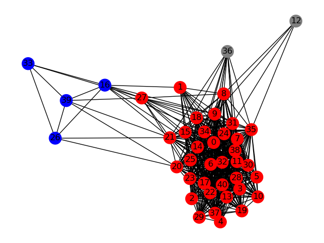
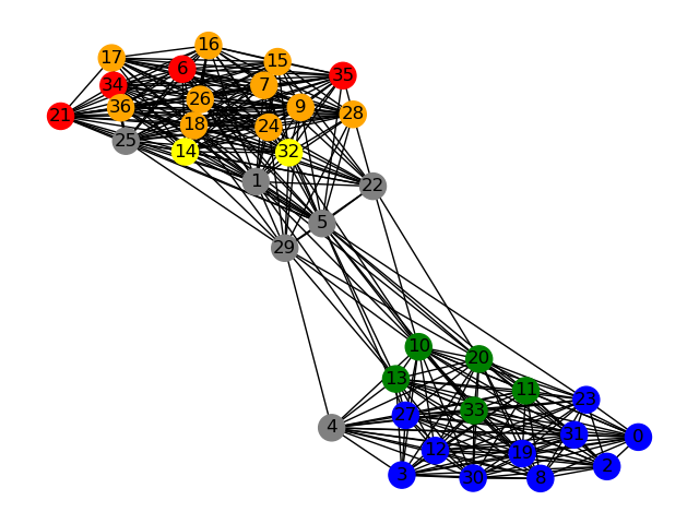

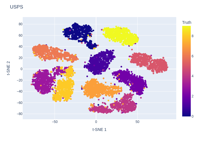
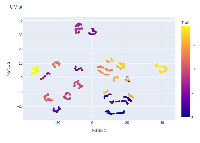


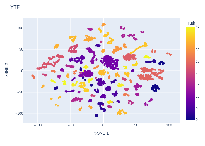
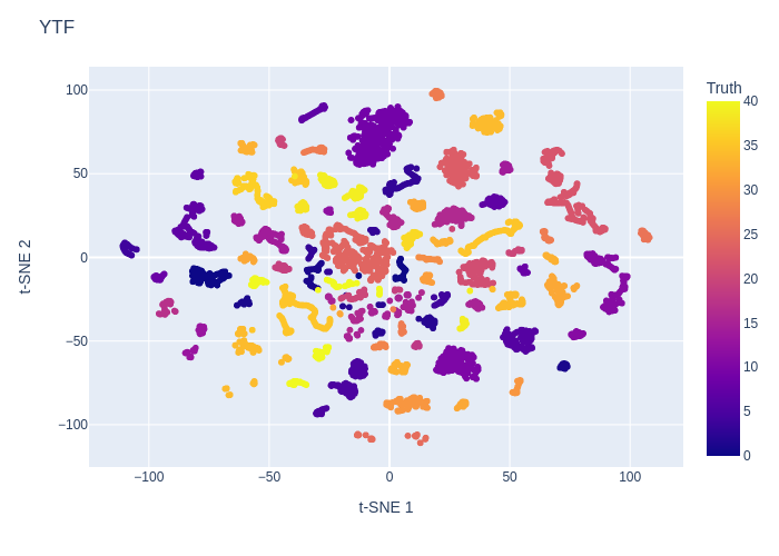
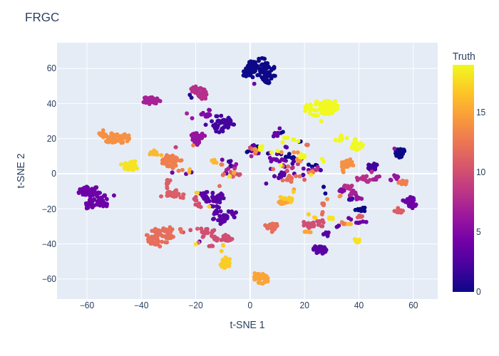
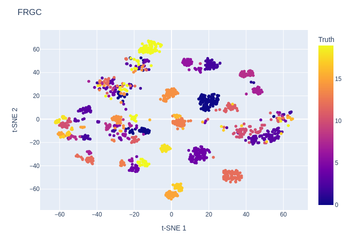

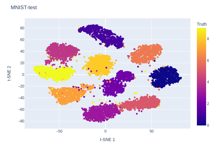
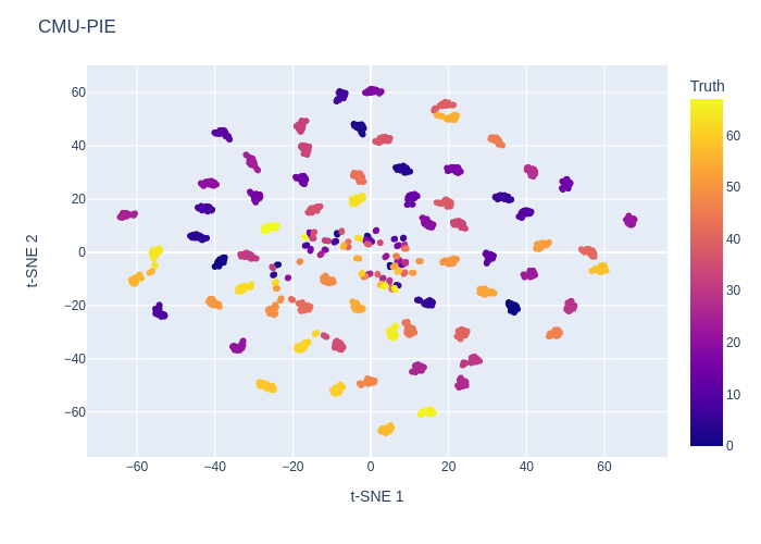

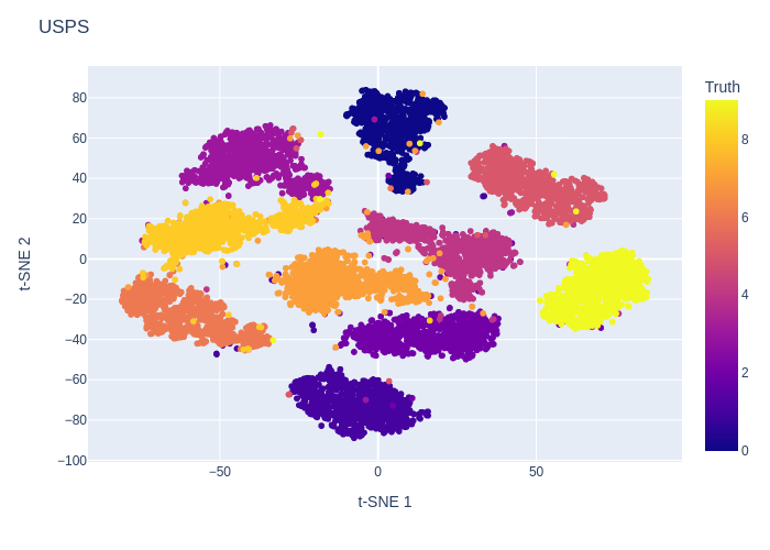
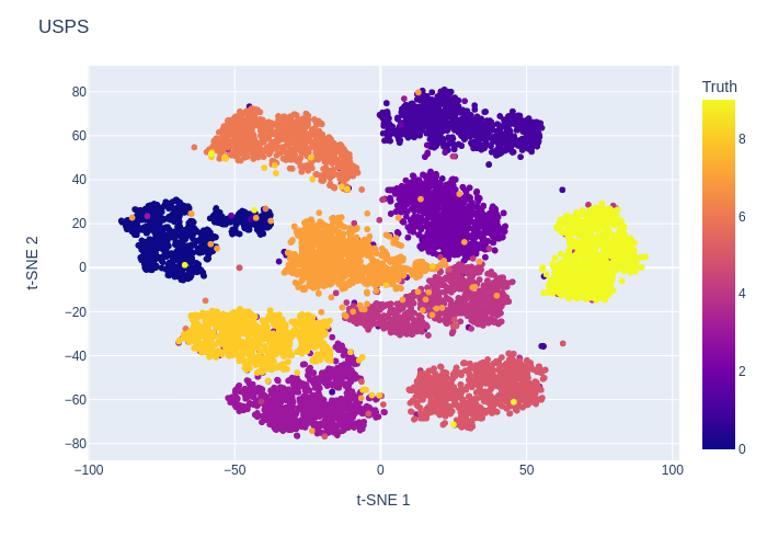


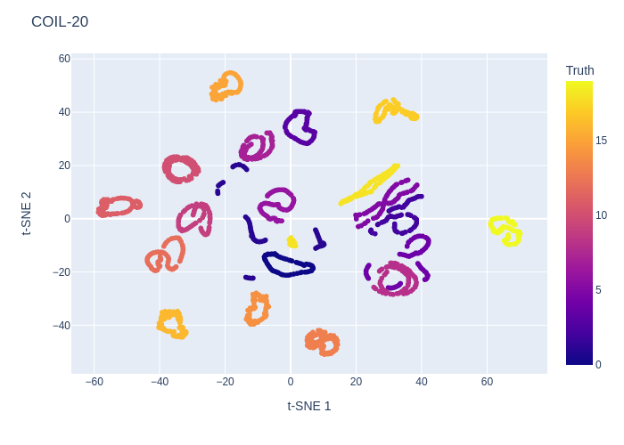
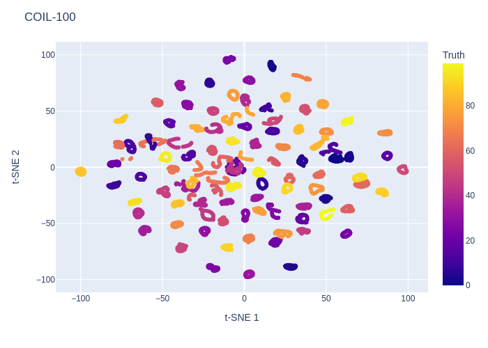
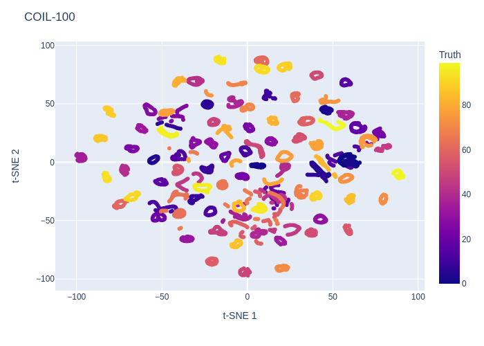
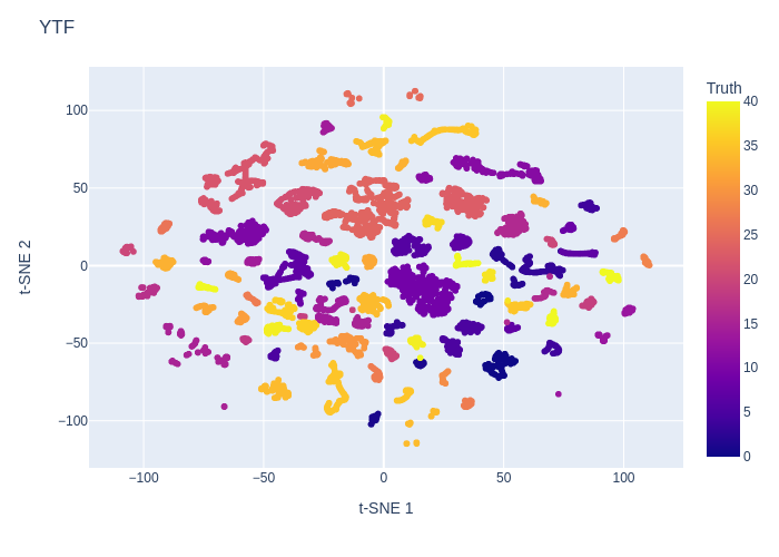
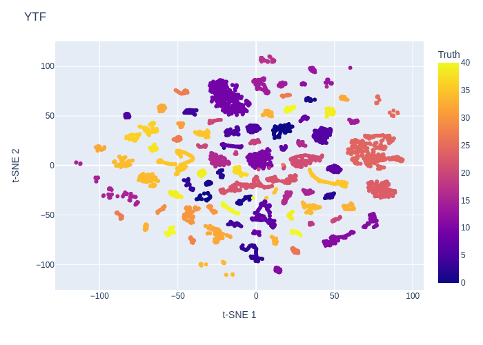
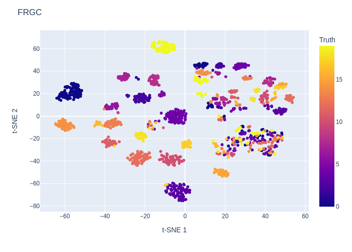
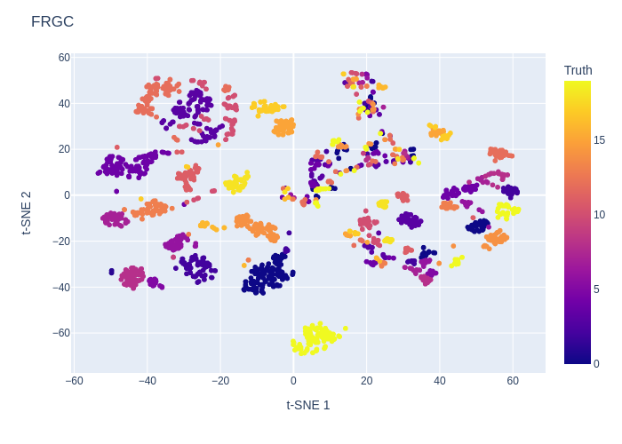
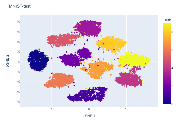
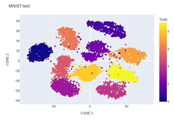
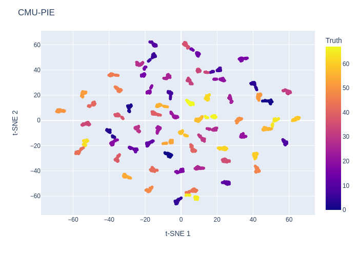


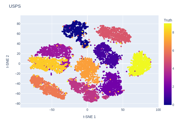

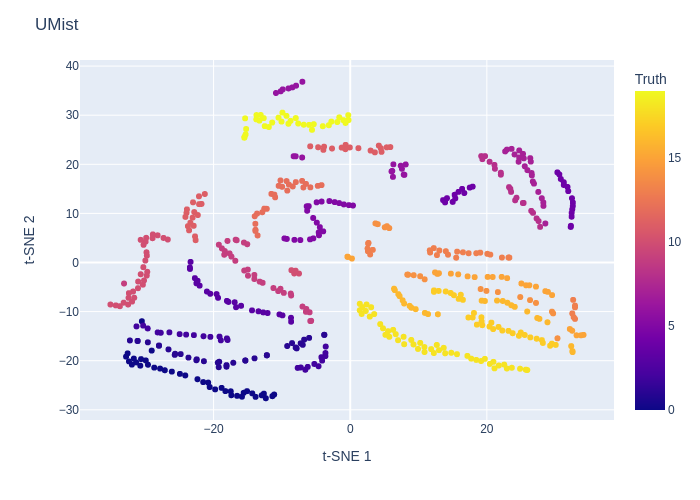
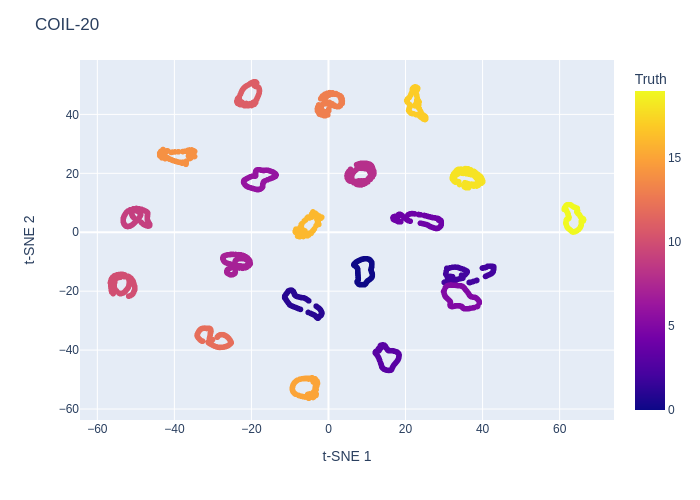
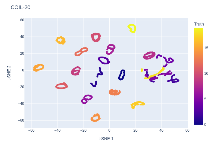
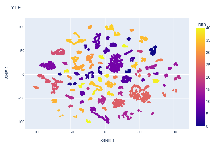
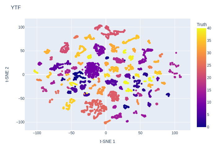
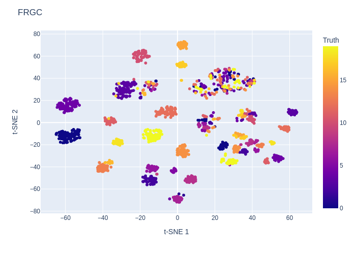
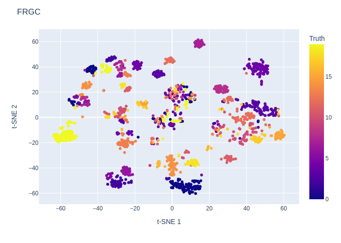

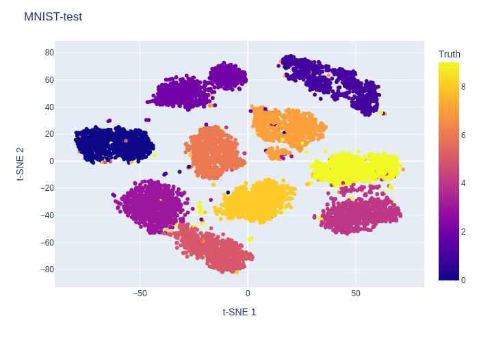


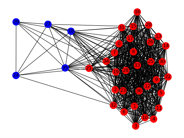
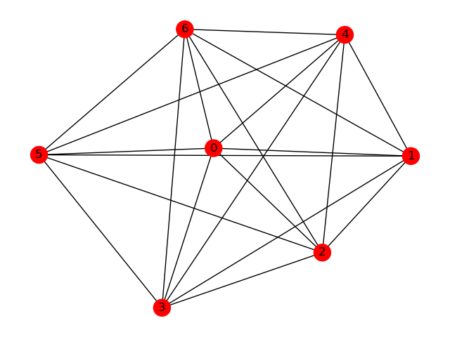
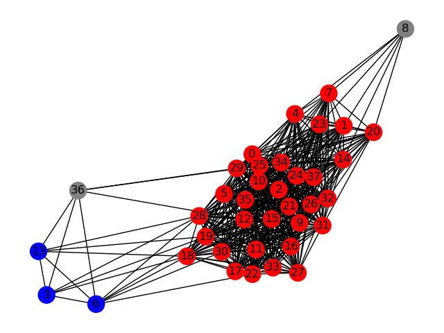
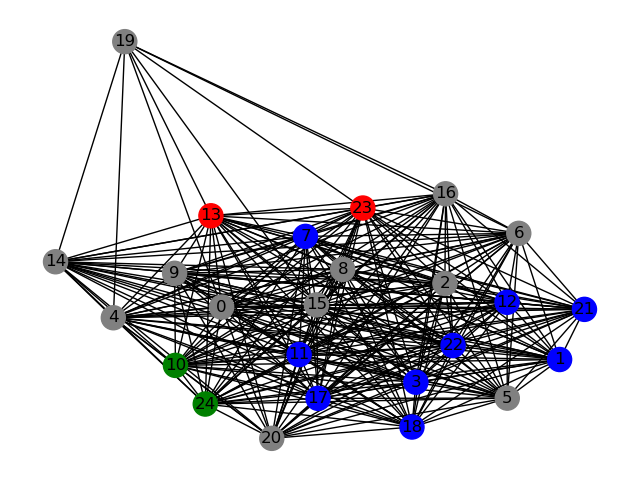
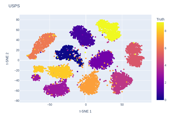


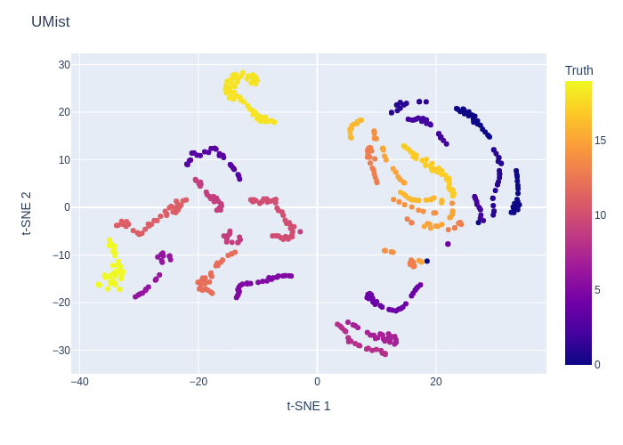


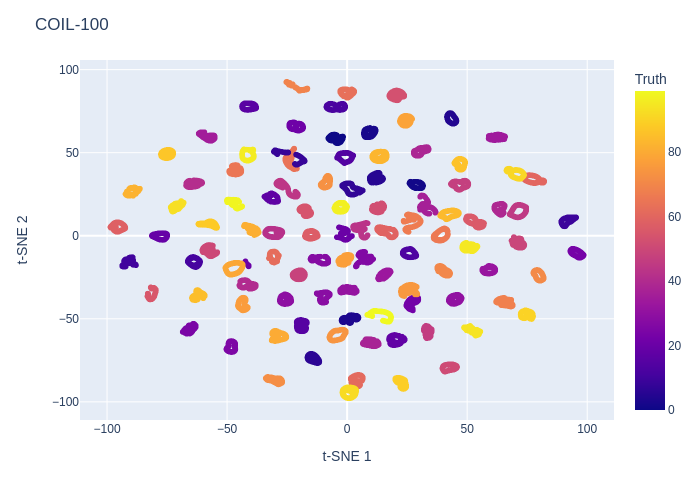
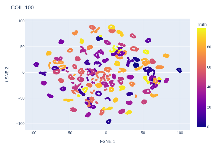


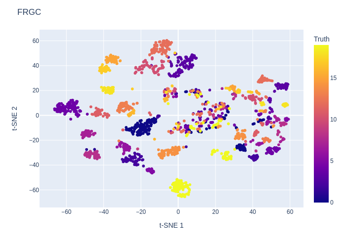


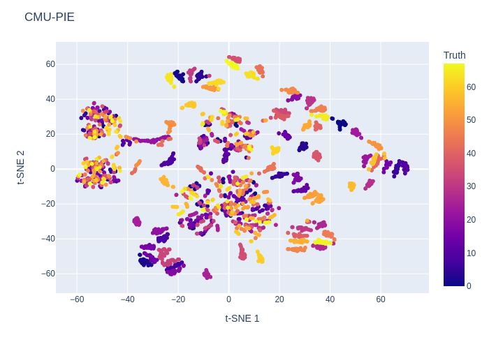
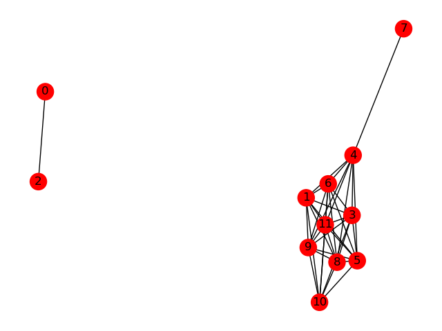
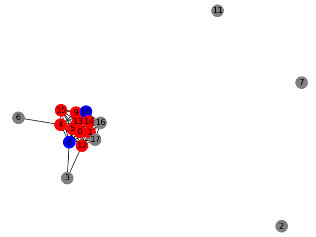
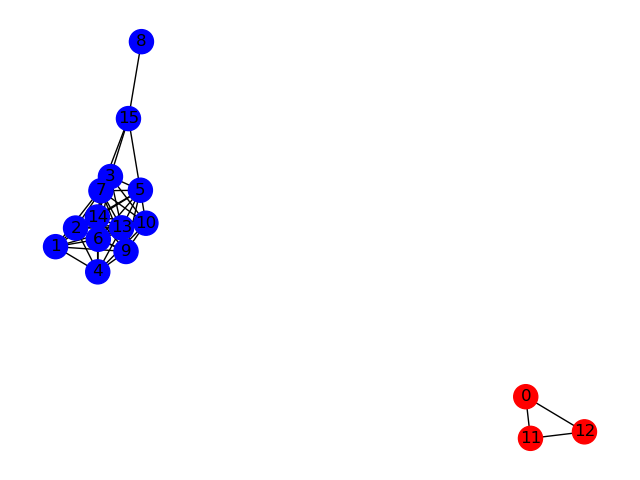
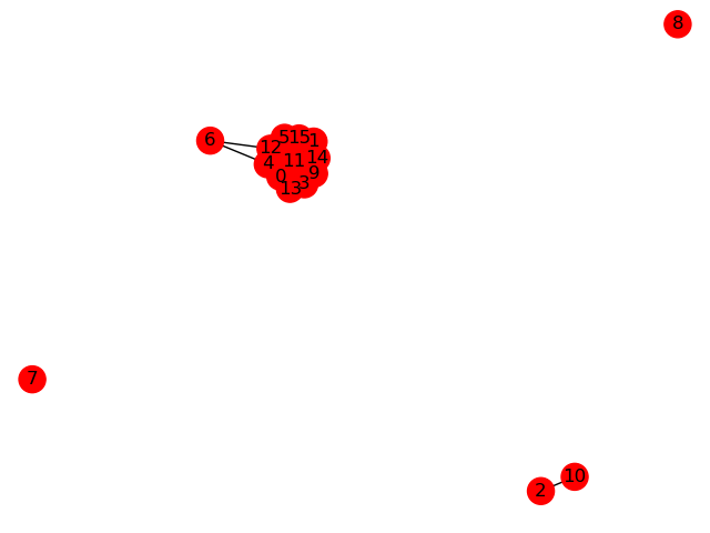
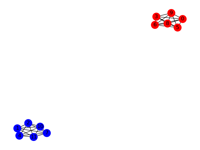
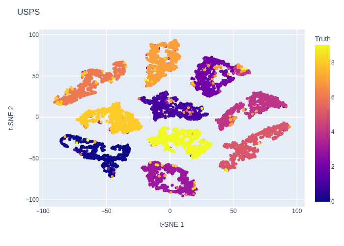

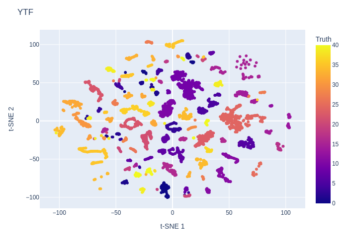
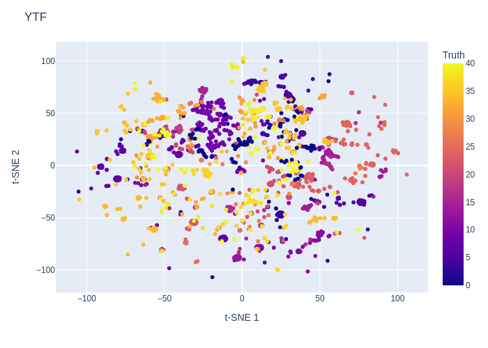
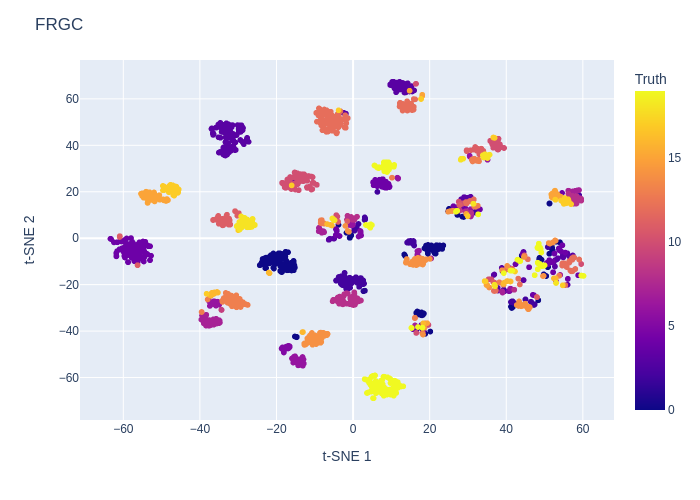
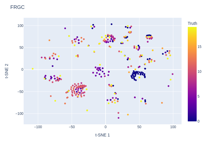


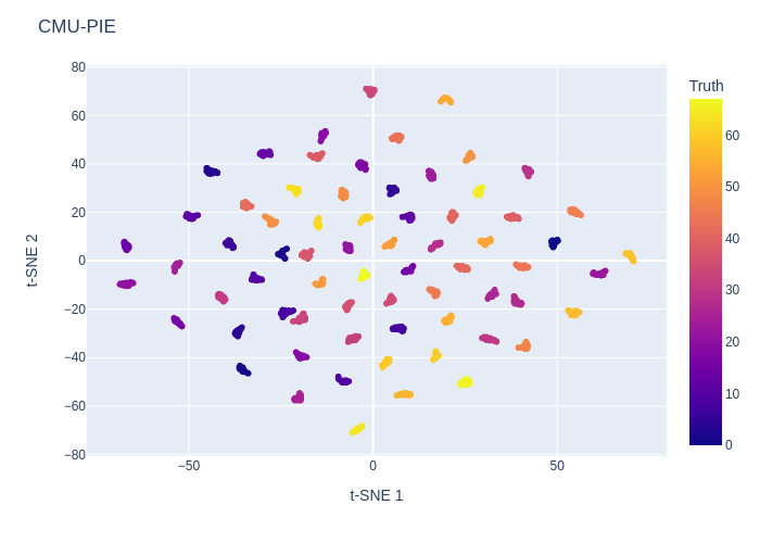

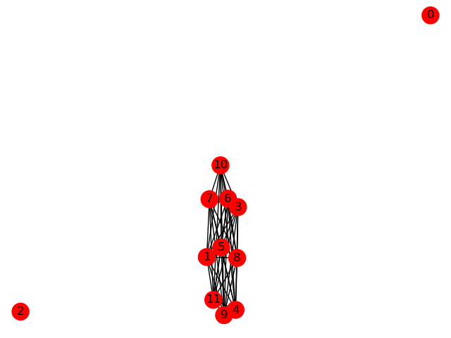
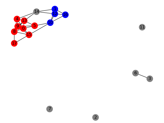
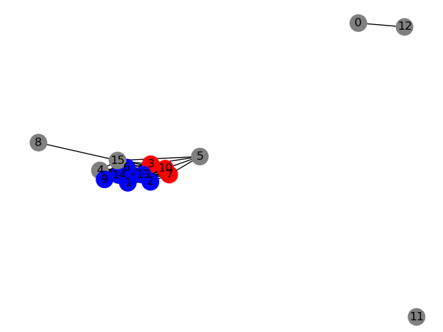
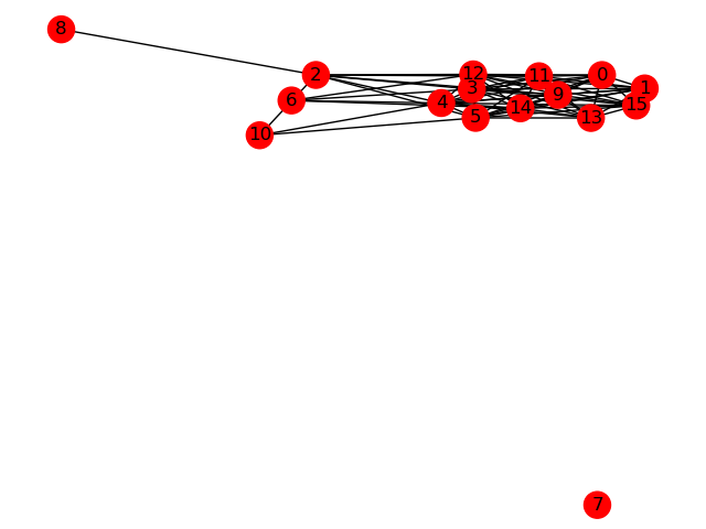
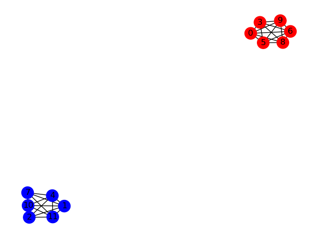
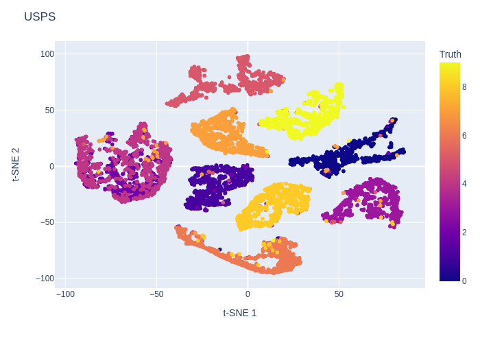

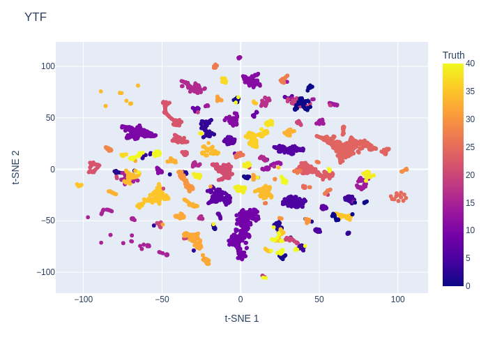


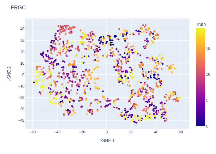


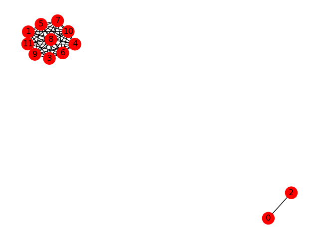
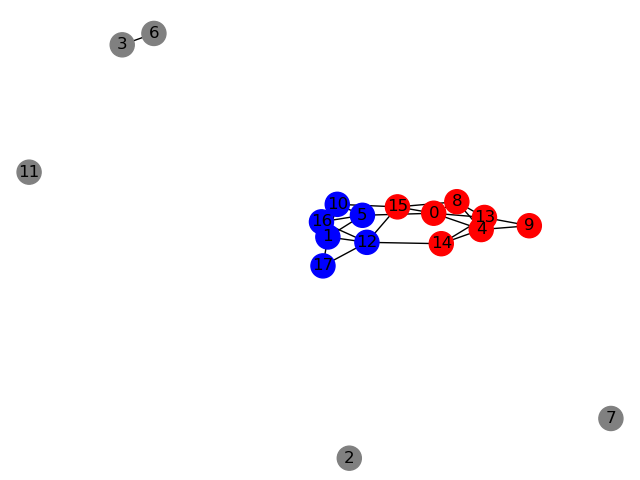
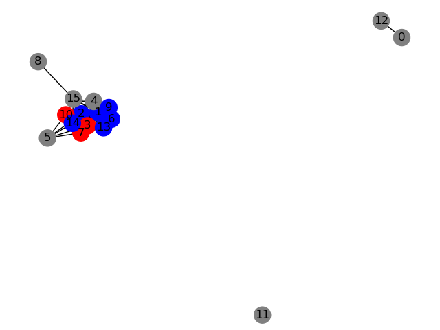
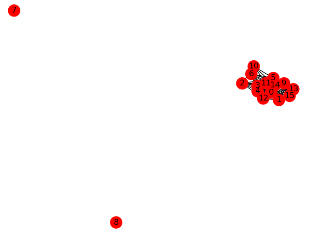
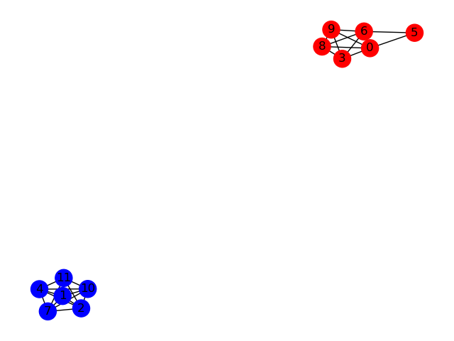


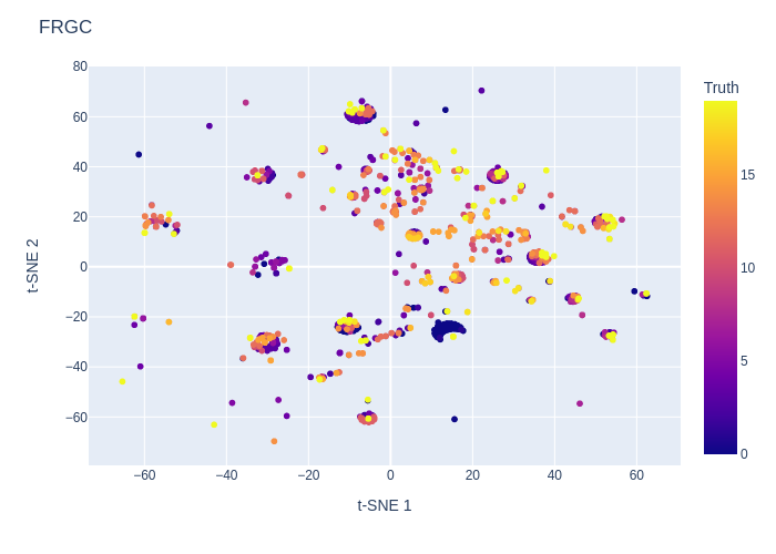
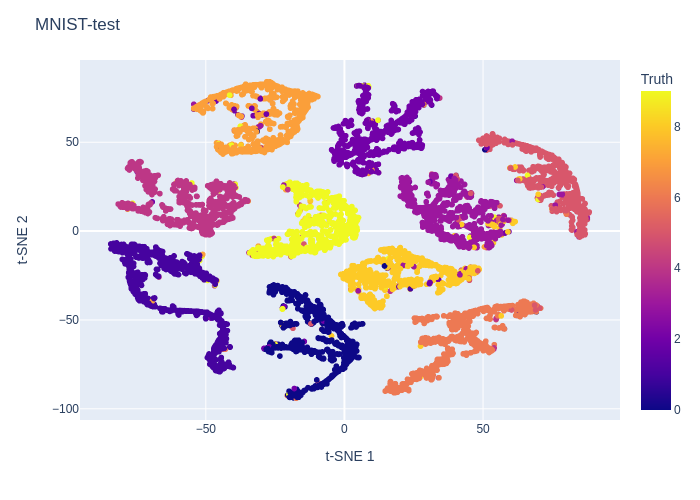
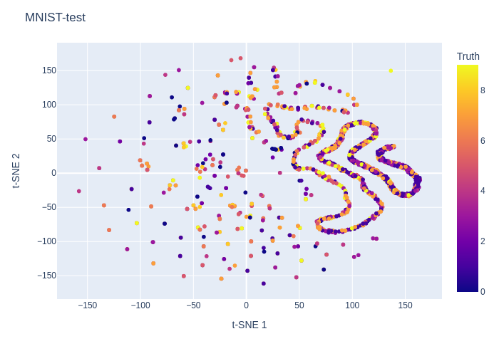

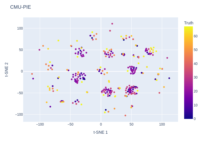
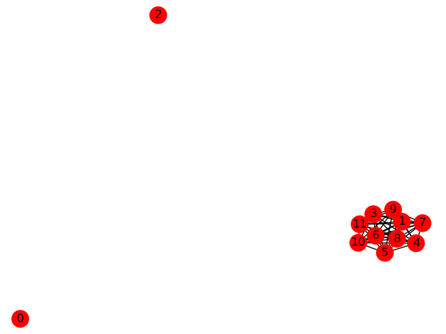
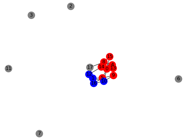
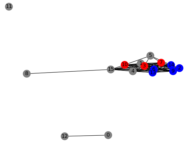
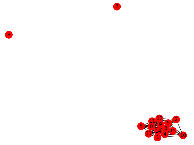
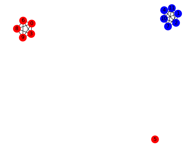
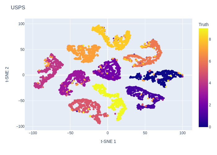
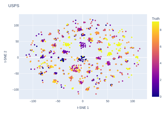
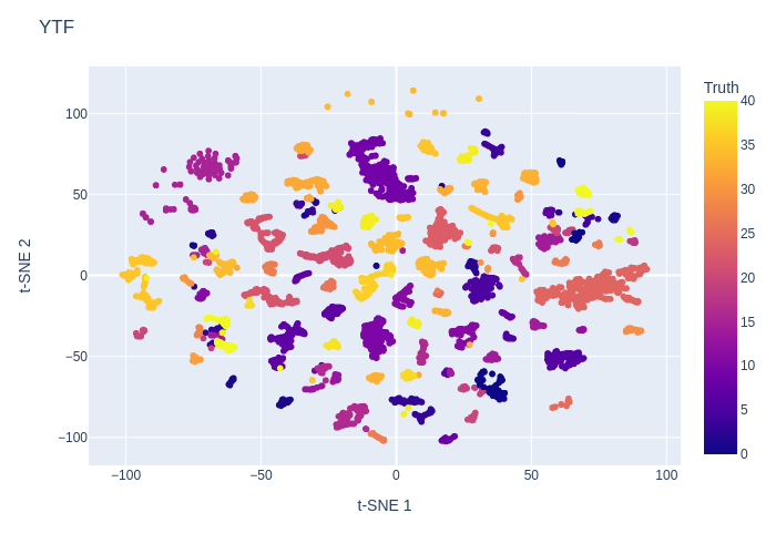

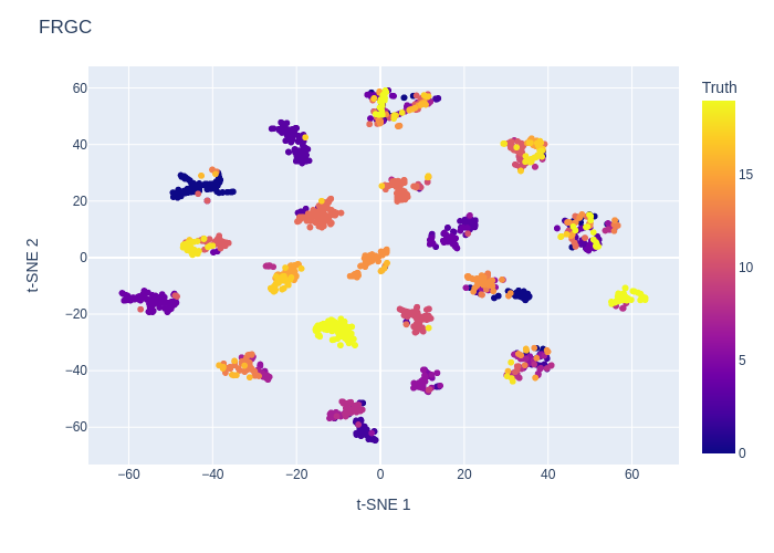

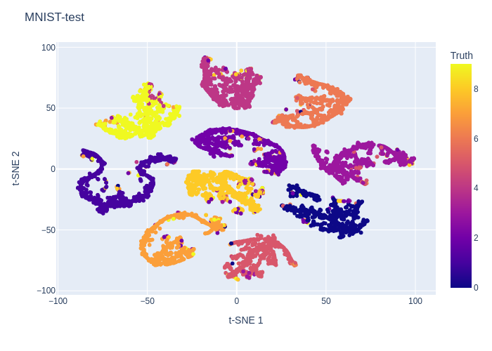


Determination of the number of clusters - NMI
In this section, we explore additional results for the hyperparameter tuning task, specifically concentrating on the rank correlation between measure scores and Normalized Mutual Information (NMI). The evaluated validity indices, including Cubic Clustering Criterion (CCC), Dunn index, Cindex, SDbw index, and CDbw index, are presented in Table 7. Both ACE and pooled scores demonstrate superior rank correlation with NMI compared to paired scores across most cases. The prevalence of missing values for raw scores underscores the practical challenges associated with obtaining them due to computational resource constraints. It is important to note that in some instances, ACE scores and pooled scores may not outperform paired scores, particularly when all three exhibit negative rank correlation with NMI, suggesting the absence of admissible spaces for this metric in the dataset.
| USPS (10) | YTF (41) | FRGC (20) | MNIST-test (10) | CMU-PIE (68) | UMist (20) | COIL-20 (20) | COIL-100 (100) | Average | ||||||||||
| JULE: Cubic clustering criterion | ||||||||||||||||||
| Raw score | - | - | - | - | - | - | - | - | - | - | - | - | - | - | - | - | - | - |
| Paired score | 0.79 (10) | 0.73 (10) | -0.22 (50) | -0.17 (50) | 0.65 (25) | 0.5 (25) | 0.82 (10) | 0.69 (10) | 0.96 (70) | 0.87 (70) | 0.33 (35) | 0.29 (35) | 0.43 (40) | 0.29 (40) | 0.69 (80) | 0.49 (80) | 0.56 | 0.46 |
| Pooled score | 0.87 (10) | 0.78 (10) | 0.78 (50) | 0.61 (50) | 0.67 (45) | 0.56 (45) | 0.84 (10) | 0.73 (10) | 0.99 (70) | 0.96 (70) | 0.24 (45) | 0.24 (45) | -0.74 (45) | -0.64 (45) | 0.64 (80) | 0.49 (80) | 0.54 | 0.47 |
| ACE | 0.87 (10) | 0.78 (10) | 0.92 (50) | 0.78 (50) | 0.53 (25) | 0.39 (25) | 0.84 (10) | 0.73 (10) | 0.99 (70) | 0.96 (70) | 0.24 (45) | 0.24 (45) | -0.67 (40) | -0.5 (40) | 0.64 (80) | 0.49 (80) | 0.55 | 0.48 |
| JULE: Dunn index | ||||||||||||||||||
| Raw score | 0.42 (10,15,35,5) | 0.4 (10,15,35,5) | -0.9 (15) | -0.78 (15) | 0.58 (25,50) | 0.42 (25,50) | 0.39 (15) | 0.33 (15) | 0.74 (100,70,80,90) | 0.65 (100,70,80,90) | - | - | 0.64 (20) | 0.57 (20) | - | - | 0.31 | 0.26 |
| Paired score | 0.28 (5) | 0.29 (5) | -0.48 (25) | -0.33 (25) | 0.6 (50) | 0.5 (50) | 0.44 (15) | 0.42 (15) | 0.55 (50) | 0.38 (50) | -0.2 (5) | -0.11 (5) | 0.64 (15) | 0.5 (15) | 0.12 (60) | 0.11 (60) | 0.24 | 0.22 |
| Pooled score | 0.43 (5) | 0.51 (5) | -0.93 (11) | -0.83 (11) | -0.4 (10) | -0.33 (10) | 0.14 (5) | 0.16 (5) | -0.27 (50) | -0.16 (50) | 0.02 (5) | 0.07 (5) | 0.48 (15) | 0.36 (15) | -0.39 (60) | -0.2 (60) | -0.11 | -0.05 |
| ACE | 0.43 (5) | 0.51 (5) | -0.98 (11) | -0.94 (11) | -0.2 (20) | -0.06 (20) | 0.14 (5) | 0.16 (5) | -0.27 (50) | -0.16 (50) | 0.02 (5) | 0.07 (5) | 0.38 (15) | 0.29 (15) | -0.44 (60) | -0.24 (60) | -0.12 | -0.05 |
| JULE: Cindex | ||||||||||||||||||
| Raw score | -0.41 (40) | -0.47 (40) | -0.02 (40) | 0.11 (40) | 0.75 (35) | 0.56 (35) | -0.19 (30) | -0.11 (30) | 0.77 (100) | 0.56 (100) | - | - | -0.69 (50) | -0.57 (50) | - | - | 0.04 | 0.01 |
| Paired score | -0.12 (45) | -0.16 (45) | -0.5 (11) | -0.39 (11) | 0.47 (30) | 0.39 (30) | -0.03 (30) | 0.02 (30) | -0.56 (20) | -0.38 (20) | 0.07 (45) | 0.16 (45) | -0.43 (50) | -0.36 (50) | 0.55 (140) | 0.38 (140) | -0.07 | -0.04 |
| Pooled score | -0.44 (45) | -0.56 (45) | 0.88 (50) | 0.72 (50) | 0.98 (50) | 0.94 (50) | -0.34 (40) | -0.38 (40) | 0.77 (100) | 0.6 (100) | 0.12 (50) | 0.02 (50) | -0.59 (50) | -0.5 (50) | 0.44 (200) | 0.29 (200) | 0.23 | 0.14 |
| ACE | -0.42 (45) | -0.51 (45) | 0.63 (25) | 0.5 (25) | 0.98 (50) | 0.94 (50) | -0.34 (40) | -0.38 (40) | 0.76 (100) | 0.56 (100) | 0.13 (50) | 0.07 (50) | -0.59 (50) | -0.5 (50) | 0.39 (200) | 0.2 (200) | 0.19 | 0.11 |
| JULE: SDbw index | ||||||||||||||||||
| Raw score | -0.37 (50) | -0.42 (50) | -0.41 (15) | -0.35 (15) | 0.82 (50) | 0.72 (50) | -0.46 (45) | -0.42 (45) | 0.6 (100) | 0.38 (100) | - | - | -0.91 (45) | -0.79 (45) | - | - | -0.12 | -0.15 |
| Paired score | -0.16 (45) | -0.16 (45) | 0.75 (35) | 0.67 (35) | 0.97 (50) | 0.89 (50) | -0.18 (50) | -0.24 (50) | 0.65 (100) | 0.51 (100) | 0.2 (45) | 0.16 (45) | -0.24 (40) | -0.21 (40) | -0.93 (20) | -0.82 (20) | 0.13 | 0.10 |
| Pooled score | -0.43 (45) | -0.51 (45) | 0.98 (50) | 0.94 (50) | 0.98 (50) | 0.94 (50) | -0.39 (45) | -0.42 (45) | 0.77 (100) | 0.56 (100) | 0.19 (50) | 0.16 (50) | -0.74 (50) | -0.64 (50) | -0.99 (20) | -0.96 (20) | 0.05 | 0.01 |
| ACE | -0.43 (45) | -0.51 (45) | 0.98 (50) | 0.94 (50) | 0.98 (50) | 0.94 (50) | -0.39 (45) | -0.42 (45) | 0.77 (100) | 0.56 (100) | 0.19 (50) | 0.16 (50) | -0.74 (50) | -0.64 (50) | -0.99 (20) | -0.96 (20) | 0.05 | 0.01 |
| JULE: CDbw index | ||||||||||||||||||
| Raw score | - | - | - | - | - | - | - | - | - | - | - | - | - | - | - | - | - | - |
| Paired score | 0.01 (15) | -0.02 (15) | -0.25 (30) | -0.11 (30) | 0.82 (45) | 0.61 (45) | -0.19 (45) | -0.16 (45) | -0.52 (20) | -0.33 (20) | 0.09 (45) | 0.11 (45) | 0.26 (15) | 0.14 (15) | -0.73 (20) | -0.6 (20) | -0.06 | -0.04 |
| Pooled score | -0.38 (50) | -0.47 (50) | 0.95 (50) | 0.89 (50) | 0.97 (50) | 0.89 (50) | -0.37 (45) | -0.33 (45) | 0.89 (70) | 0.78 (70) | 0.31 (45) | 0.24 (45) | 0.52 (15) | 0.43 (15) | -0.41 (20) | -0.24 (20) | 0.31 | 0.27 |
| ACE | -0.37 (45) | -0.42 (45) | 0.98 (50) | 0.94 (50) | 0.97 (50) | 0.89 (50) | -0.37 (45) | -0.33 (45) | 0.88 (70) | 0.73 (70) | 0.31 (45) | 0.24 (45) | 0.57 (15) | 0.5 (15) | -0.39 (20) | -0.2 (20) | 0.32 | 0.29 |
| DEPICT: Cubic clustering criterion | ||||||||||||||||||
| Raw score | - | - | - | - | - | - | - | - | - | - | - | - | ||||||
| Paired score | -0.19 (25) | -0.11 (25) | 0.98 (50) | 0.91 (50) | 0.53 (25) | 0.39 (25) | 0.13 (35) | 0.11 (35) | 0.98 (80) | 0.91 (80) | 0.49 | 0.44 | ||||||
| Pooled score | -0.25 (40) | -0.29 (40) | 1.0 (50) | 1.0 (50) | 0.83 (50) | 0.67 (50) | 0.1 (40) | 0.07 (40) | 0.92 (100) | 0.82 (100) | 0.52 | 0.45 | ||||||
| ACE | -0.25 (40) | -0.29 (40) | 1.0 (50) | 1.0 (50) | 0.83 (50) | 0.67 (50) | 0.06 (40) | 0.02 (40) | 0.92 (100) | 0.82 (100) | 0.51 | 0.44 | ||||||
| DEPICT: Dunn index | ||||||||||||||||||
| Raw score | -0.16 (5) | -0.11 (5) | 0.82 (50) | 0.69 (50) | 0.83 (35) | 0.67 (35) | 0.07 (10) | 0.02 (10) | 0.2 (100) | 0.24 (100) | 0.35 | 0.30 | ||||||
| Paired score | 0.04 (25) | 0.07 (25) | -0.22 (5) | -0.16 (5) | -0.57 (15) | -0.44 (15) | 0.34 (15) | 0.29 (15) | 0.02 (50) | -0.02 (50) | -0.08 | -0.05 | ||||||
| Pooled score | -0.12 (5) | -0.07 (5) | -0.32 (5) | -0.24 (5) | 0.0 (30) | 0.0 (30) | 0.24 (10) | 0.2 (10) | 0.22 (50) | 0.16 (50) | 0.00 | 0.01 | ||||||
| ACE | -0.38 (5) | -0.29 (5) | 0.04 (15) | 0.02 (15) | 0.0 (30) | 0.0 (30) | 0.24 (5) | 0.24 (5) | 0.22 (50) | 0.16 (50) | 0.02 | 0.03 | ||||||
| DEPICT: Cindex | ||||||||||||||||||
| Raw score | -0.22 (40) | -0.24 (40) | 0.65 (35) | 0.42 (35) | 0.72 (40) | 0.56 (40) | -0.42 (45) | -0.38 (45) | 0.85 (100) | 0.73 (100) | 0.32 | 0.22 | ||||||
| Paired score | 0.46 (5) | 0.6 (5) | -0.54 (5) | -0.47 (5) | -0.92 (10) | -0.83 (10) | 0.42 (5) | 0.47 (5) | 0.12 (10) | 0.16 (10) | -0.09 | -0.01 | ||||||
| Pooled score | -0.44 (50) | -0.56 (50) | 1.0 (50) | 1.0 (50) | 0.85 (50) | 0.72 (50) | -0.37 (50) | -0.42 (50) | 0.92 (100) | 0.82 (100) | 0.39 | 0.31 | ||||||
| ACE | -0.44 (50) | -0.56 (50) | 1.0 (50) | 1.0 (50) | 0.78 (50) | 0.61 (50) | -0.37 (50) | -0.42 (50) | 0.92 (100) | 0.82 (100) | 0.38 | 0.29 | ||||||
| DEPICT: SDbw index | ||||||||||||||||||
| Raw score | -0.41 (45) | -0.47 (45) | -0.51 (15) | -0.4 (15) | 0.72 (50) | 0.5 (50) | -0.36 (40) | -0.38 (40) | 0.92 (100) | 0.82 (100) | 0.07 | 0.01 | ||||||
| Paired score | 0.43 (5) | 0.51 (5) | -0.41 (5) | -0.29 (5) | -0.85 (10) | -0.72 (10) | 0.55 (10) | 0.6 (10) | 0.26 (10) | 0.29 (10) | -0.00 | 0.08 | ||||||
| Pooled score | -0.44 (50) | -0.56 (50) | 1.0 (50) | 1.0 (50) | 0.85 (50) | 0.72 (50) | -0.34 (45) | -0.38 (45) | 0.92 (100) | 0.82 (100) | 0.40 | 0.32 | ||||||
| ACE | -0.44 (50) | -0.56 (50) | 1.0 (50) | 1.0 (50) | 0.85 (50) | 0.72 (50) | -0.38 (45) | -0.47 (45) | 0.93 (100) | 0.87 (100) | 0.39 | 0.31 | ||||||
| DEPICT: CDbw index | ||||||||||||||||||
| Raw score | - | - | - | - | - | - | - | - | -0.43 (20) | -0.38 (20) | -0.43 | -0.38 | ||||||
| Paired score | 0.42 (5) | 0.51 (5) | -0.72 (5) | -0.6 (5) | -0.83 (10) | -0.67 (10) | 0.44 (5) | 0.56 (5) | -0.81 (10) | -0.64 (10) | -0.30 | -0.17 | ||||||
| Pooled score | -0.55 (50) | -0.47 (50) | -0.07 (5) | 0.07 (5) | -0.9 (10) | -0.78 (10) | -0.76 (5) | -0.56 (5) | 0.85 (100) | 0.73 (100) | -0.29 | -0.20 | ||||||
| ACE | -0.01 (50) | -0.11 (50) | 0.39 (5) | 0.42 (5) | -0.25 (10) | -0.17 (10) | -0.73 (5) | -0.51 (5) | 0.9 (100) | 0.78 (100) | 0.06 | 0.08 | ||||||
Determination of the number of clusters - ACC
In this section, we present the rank correlation between different scores and clustering accuracy (ACC) across all validity indices, detailed in Table 8 and Table 9. The findings are consistent with our observations in Tables 2 and 7, which assess performance using NMI, thereby reinforcing our conclusions regarding the evaluation of deep clustering using these four scores.
| USPS (10) | YTF (41) | FRGC (20) | MNIST-test (10) | CMU-PIE (68) | UMist (20) | COIL-20 (20) | COIL-100 (100) | Average | ||||||||||
| JULE: Davies-Bouldin index | ||||||||||||||||||
| Raw score | -0.49 | -0.38 | 0.85 | 0.67 | 0.37 | 0.20 | -0.41 | -0.38 | 0.77 | 0.51 | 0.02 | -0.16 | -0.86 | -0.71 | -0.82 | -0.78 | -0.07 | -0.13 |
| Paired score | 0.39 | 0.29 | 0.10 | 0.06 | 0.37 | 0.25 | 0.49 | 0.33 | 0.83 | 0.60 | -0.28 | -0.29 | -0.29 | -0.21 | -0.87 | -0.73 | 0.09 | 0.04 |
| Pooled score | 0.89 | 0.73 | 0.80 | 0.67 | 0.71 | 0.54 | 0.83 | 0.64 | 0.85 | 0.69 | -0.42 | -0.33 | -0.79 | -0.64 | -0.79 | -0.69 | 0.26 | 0.20 |
| ACE | 0.89 | 0.73 | 0.80 | 0.67 | 0.60 | 0.42 | 0.83 | 0.64 | 0.88 | 0.73 | -0.42 | -0.33 | -0.71 | -0.64 | -0.82 | -0.69 | 0.26 | 0.19 |
| JULE: Calinski-Harabasz index | ||||||||||||||||||
| Raw score | 0.71 | 0.64 | 1.00 | 1.00 | -0.46 | -0.25 | 0.41 | 0.47 | -0.38 | -0.29 | -0.09 | -0.02 | 0.76 | 0.71 | 0.36 | 0.33 | 0.29 | 0.32 |
| Paired score | 0.84 | 0.73 | 0.03 | -0.06 | -0.49 | -0.31 | 0.61 | 0.56 | -0.09 | -0.07 | -0.04 | 0.07 | 0.74 | 0.64 | 0.60 | 0.51 | 0.27 | 0.26 |
| Pooled score | 0.84 | 0.73 | 0.88 | 0.78 | -0.37 | -0.20 | 0.61 | 0.56 | 0.85 | 0.69 | -0.07 | 0.02 | 0.76 | 0.71 | 0.56 | 0.51 | 0.51 | 0.48 |
| ACE | 0.84 | 0.73 | 0.92 | 0.83 | -0.11 | -0.03 | 0.61 | 0.56 | 0.83 | 0.69 | -0.07 | 0.02 | 0.76 | 0.71 | 0.65 | 0.56 | 0.55 | 0.51 |
| JULE: Silhouette score (cosine distance) | ||||||||||||||||||
| Raw score | 0.58 | 0.42 | 0.95 | 0.89 | 0.52 | 0.42 | -0.01 | -0.02 | -0.32 | -0.16 | 0.08 | 0.02 | -0.50 | -0.36 | 0.53 | 0.38 | 0.23 | 0.20 |
| Paired score | 0.89 | 0.78 | 0.27 | 0.22 | 0.21 | 0.09 | 0.81 | 0.64 | 0.99 | 0.96 | -0.26 | -0.24 | 0.55 | 0.43 | 0.52 | 0.33 | 0.50 | 0.40 |
| Pooled score | 0.95 | 0.87 | 0.98 | 0.94 | 0.61 | 0.48 | 0.94 | 0.82 | 0.99 | 0.96 | -0.32 | -0.24 | 0.67 | 0.50 | 0.54 | 0.38 | 0.67 | 0.59 |
| ACE | 0.95 | 0.87 | 0.98 | 0.94 | 0.64 | 0.54 | 0.94 | 0.82 | 0.99 | 0.96 | -0.32 | -0.24 | 0.76 | 0.57 | 0.60 | 0.47 | 0.69 | 0.61 |
| JULE: Silhouette score (euclidean distance) | ||||||||||||||||||
| Raw score | 0.62 | 0.56 | 0.95 | 0.89 | -0.17 | -0.14 | 0.53 | 0.42 | 0.53 | 0.33 | 0.04 | -0.07 | -0.38 | -0.29 | 0.52 | 0.33 | 0.33 | 0.25 |
| Paired score | 0.93 | 0.82 | 0.30 | 0.28 | 0.21 | 0.09 | 0.82 | 0.64 | 0.98 | 0.91 | -0.13 | -0.16 | 0.52 | 0.36 | 0.55 | 0.42 | 0.52 | 0.42 |
| Pooled score | 0.95 | 0.87 | 0.97 | 0.89 | 0.61 | 0.48 | 0.92 | 0.78 | 0.99 | 0.96 | -0.03 | -0.11 | 0.74 | 0.50 | 0.59 | 0.47 | 0.72 | 0.60 |
| ACE | 0.95 | 0.87 | 0.98 | 0.94 | 0.57 | 0.48 | 0.92 | 0.78 | 0.99 | 0.96 | -0.03 | -0.11 | 0.74 | 0.50 | 0.59 | 0.47 | 0.71 | 0.61 |
| JULE: Cubic clustering criterion | ||||||||||||||||||
| Raw score | - | - | - | - | - | - | - | - | - | - | - | - | - | - | - | - | - | - |
| Paired score | 0.90 | 0.82 | -0.28 | -0.28 | 0.26 | 0.14 | 0.77 | 0.64 | 0.93 | 0.82 | 0.13 | 0.07 | 0.45 | 0.36 | 0.52 | 0.36 | 0.46 | 0.37 |
| Pooled score | 0.94 | 0.87 | 0.77 | 0.61 | 0.51 | 0.37 | 0.81 | 0.69 | 1.00 | 1.00 | 0.04 | -0.07 | -0.71 | -0.57 | 0.47 | 0.36 | 0.48 | 0.41 |
| ACE | 0.94 | 0.87 | 0.92 | 0.78 | 0.39 | 0.31 | 0.81 | 0.69 | 1.00 | 1.00 | 0.04 | -0.07 | -0.69 | -0.57 | 0.47 | 0.36 | 0.48 | 0.42 |
| JULE: Dunn index | ||||||||||||||||||
| Raw score | 0.71 | 0.60 | -0.83 | -0.67 | 0.31 | 0.23 | 0.42 | 0.38 | 0.78 | 0.69 | - | - | 0.62 | 0.50 | - | - | 0.33 | 0.29 |
| Paired score | 0.52 | 0.38 | -0.40 | -0.22 | 0.09 | 0.09 | 0.49 | 0.47 | 0.50 | 0.33 | -0.28 | -0.24 | 0.67 | 0.57 | -0.03 | -0.02 | 0.19 | 0.17 |
| Pooled score | 0.69 | 0.60 | -0.85 | -0.72 | -0.35 | -0.20 | 0.20 | 0.20 | -0.37 | -0.20 | -0.07 | -0.07 | 0.52 | 0.43 | -0.54 | -0.33 | -0.10 | -0.04 |
| ACE | 0.69 | 0.60 | -0.93 | -0.83 | -0.31 | -0.25 | 0.20 | 0.20 | -0.37 | -0.20 | -0.07 | -0.07 | 0.45 | 0.36 | -0.59 | -0.38 | -0.12 | -0.07 |
| JULE: Cindex | ||||||||||||||||||
| Raw score | -0.71 | -0.64 | 0.17 | 0.22 | 0.07 | 0.09 | -0.21 | -0.16 | 0.83 | 0.60 | - | - | -0.71 | -0.64 | - | - | -0.09 | -0.09 |
| Paired score | -0.36 | -0.24 | -0.58 | -0.50 | 0.14 | 0.20 | -0.04 | -0.02 | -0.60 | -0.42 | -0.06 | -0.07 | -0.48 | -0.43 | 0.60 | 0.42 | -0.17 | -0.13 |
| Pooled score | -0.72 | -0.64 | 0.87 | 0.72 | 0.45 | 0.31 | -0.33 | -0.33 | 0.78 | 0.64 | 0.04 | -0.11 | -0.64 | -0.57 | 0.55 | 0.42 | 0.12 | 0.05 |
| ACE | -0.70 | -0.60 | 0.58 | 0.39 | 0.45 | 0.31 | -0.33 | -0.33 | 0.77 | 0.60 | 0.06 | -0.07 | -0.64 | -0.57 | 0.52 | 0.33 | 0.09 | 0.01 |
| JULE: SDbw index | ||||||||||||||||||
| Raw score | -0.61 | -0.51 | -0.41 | -0.35 | 0.18 | 0.09 | -0.41 | -0.38 | 0.66 | 0.42 | - | - | -0.88 | -0.71 | - | - | -0.24 | -0.24 |
| Paired score | -0.42 | -0.24 | 0.78 | 0.67 | 0.35 | 0.25 | -0.15 | -0.20 | 0.71 | 0.56 | 0.01 | -0.16 | -0.29 | -0.29 | -0.95 | -0.87 | 0.01 | -0.03 |
| Pooled score | -0.70 | -0.60 | 0.92 | 0.83 | 0.45 | 0.31 | -0.36 | -0.38 | 0.82 | 0.60 | 0.02 | -0.16 | -0.76 | -0.71 | -0.96 | -0.91 | -0.07 | -0.13 |
| ACE | -0.70 | -0.60 | 0.92 | 0.83 | 0.45 | 0.31 | -0.36 | -0.38 | 0.82 | 0.60 | 0.02 | -0.16 | -0.76 | -0.71 | -0.96 | -0.91 | -0.07 | -0.13 |
| JULE: CDbw index | ||||||||||||||||||
| Raw score | - | - | - | - | - | - | - | - | - | - | - | - | - | - | - | - | - | - |
| Paired score | -0.20 | -0.11 | -0.23 | -0.11 | 0.59 | 0.42 | -0.13 | -0.11 | -0.55 | -0.38 | -0.15 | -0.20 | 0.24 | 0.07 | -0.81 | -0.64 | -0.16 | -0.13 |
| Pooled score | -0.65 | -0.56 | 0.87 | 0.78 | 0.54 | 0.37 | -0.31 | -0.29 | 0.90 | 0.82 | 0.06 | -0.07 | 0.43 | 0.36 | -0.53 | -0.38 | 0.16 | 0.13 |
| ACE | -0.64 | -0.51 | 0.92 | 0.83 | 0.54 | 0.37 | -0.31 | -0.29 | 0.89 | 0.78 | 0.06 | -0.07 | 0.48 | 0.43 | -0.52 | -0.33 | 0.18 | 0.15 |
| DEPICT: Davies-Bouldin index | ||||||||||||||||||
| Raw score | -0.82 | -0.64 | 1.00 | 1.00 | 0.03 | -0.11 | -0.50 | -0.33 | 0.92 | 0.82 | 0.13 | 0.15 | ||||||
| Paired score | 0.88 | 0.82 | -0.77 | -0.60 | -0.37 | -0.22 | 0.79 | 0.73 | -0.10 | 0.02 | 0.09 | 0.15 | ||||||
| Pooled score | 0.90 | 0.73 | 0.90 | 0.78 | 0.47 | 0.33 | 0.88 | 0.82 | 0.92 | 0.82 | 0.81 | 0.70 | ||||||
| ACE | 0.93 | 0.82 | 0.96 | 0.91 | 0.92 | 0.83 | 0.93 | 0.87 | 0.96 | 0.91 | 0.94 | 0.87 | ||||||
| USPS (10) | YTF (41) | FRGC (20) | MNIST-test (10) | CMU-PIE (68) | UMist (20) | COIL-20 (20) | COIL-100 (100) | Average | ||||||||||
| DEPICT: Calinski-Harabasz index | ||||||||||||||||||
| Raw score | 0.88 | 0.82 | -0.66 | -0.51 | -0.40 | -0.28 | 0.82 | 0.78 | -0.92 | -0.82 | -0.06 | -0.00 | ||||||
| Paired score | 0.88 | 0.82 | -0.96 | -0.91 | -0.37 | -0.22 | 0.79 | 0.73 | -0.92 | -0.82 | -0.11 | -0.08 | ||||||
| Pooled score | 0.88 | 0.82 | -0.94 | -0.87 | -0.37 | -0.22 | 0.82 | 0.78 | 0.44 | 0.56 | 0.17 | 0.21 | ||||||
| ACE | 0.88 | 0.82 | -0.67 | -0.56 | 0.92 | 0.78 | 0.82 | 0.78 | 0.92 | 0.82 | 0.57 | 0.53 | ||||||
| DEPICT: Silhouette score (cosine distance) | ||||||||||||||||||
| Raw score | -0.39 | -0.33 | 0.99 | 0.96 | 0.52 | 0.39 | 0.76 | 0.56 | -0.43 | -0.33 | 0.29 | 0.25 | ||||||
| Paired score | 0.87 | 0.78 | -0.69 | -0.56 | -0.37 | -0.22 | 0.79 | 0.73 | 0.07 | 0.11 | 0.14 | 0.17 | ||||||
| Pooled score | 0.90 | 0.73 | 0.67 | 0.51 | 0.68 | 0.56 | 0.90 | 0.82 | 0.98 | 0.91 | 0.83 | 0.71 | ||||||
| ACE | 0.95 | 0.87 | 0.92 | 0.82 | 0.80 | 0.67 | 0.95 | 0.87 | 0.99 | 0.96 | 0.92 | 0.84 | ||||||
| DEPICT: Silhouette score (euclidean distance) | ||||||||||||||||||
| Raw score | -0.28 | -0.24 | 0.99 | 0.96 | -0.20 | -0.17 | 0.66 | 0.51 | -0.43 | -0.33 | 0.15 | 0.14 | ||||||
| Paired score | 0.87 | 0.78 | -0.64 | -0.51 | -0.37 | -0.22 | 0.79 | 0.73 | -0.12 | -0.02 | 0.11 | 0.15 | ||||||
| Pooled score | 0.90 | 0.73 | 0.99 | 0.96 | 0.68 | 0.56 | 0.94 | 0.87 | 0.99 | 0.96 | 0.90 | 0.81 | ||||||
| ACE | 0.88 | 0.82 | 0.98 | 0.91 | 0.73 | 0.56 | 0.95 | 0.87 | 0.98 | 0.91 | 0.90 | 0.81 | ||||||
| DEPICT: Cubic clustering criterion | ||||||||||||||||||
| Raw score | - | - | - | - | - | - | - | - | - | - | - | - | ||||||
| Paired score | -0.49 | -0.33 | 0.99 | 0.96 | 0.90 | 0.78 | -0.16 | -0.07 | 0.98 | 0.91 | 0.44 | 0.45 | ||||||
| Pooled score | -0.62 | -0.51 | 0.99 | 0.96 | 0.38 | 0.28 | -0.19 | -0.11 | 0.92 | 0.82 | 0.29 | 0.29 | ||||||
| ACE | -0.62 | -0.51 | 0.99 | 0.96 | 0.38 | 0.28 | -0.25 | -0.16 | 0.92 | 0.82 | 0.28 | 0.28 | ||||||
| DEPICT: Dunn index | ||||||||||||||||||
| Raw score | 0.19 | 0.11 | 0.85 | 0.73 | 0.48 | 0.39 | 0.25 | 0.20 | 0.20 | 0.24 | 0.39 | 0.34 | ||||||
| Paired score | 0.24 | 0.20 | -0.19 | -0.11 | -0.20 | -0.06 | 0.59 | 0.47 | 0.02 | -0.02 | 0.09 | 0.10 | ||||||
| Pooled score | 0.24 | 0.16 | -0.31 | -0.20 | 0.60 | 0.50 | 0.46 | 0.38 | 0.22 | 0.16 | 0.24 | 0.20 | ||||||
| ACE | -0.07 | -0.07 | 0.09 | 0.07 | 0.60 | 0.50 | 0.53 | 0.42 | 0.22 | 0.16 | 0.28 | 0.22 | ||||||
| DEPICT: Cindex | ||||||||||||||||||
| Raw score | -0.60 | -0.47 | 0.61 | 0.38 | 0.73 | 0.50 | -0.72 | -0.56 | 0.85 | 0.73 | 0.18 | 0.12 | ||||||
| Paired score | 0.88 | 0.82 | -0.62 | -0.51 | -0.43 | -0.33 | 0.78 | 0.64 | 0.12 | 0.16 | 0.14 | 0.16 | ||||||
| Pooled score | -0.87 | -0.78 | 0.99 | 0.96 | 0.37 | 0.22 | -0.70 | -0.60 | 0.92 | 0.82 | 0.14 | 0.12 | ||||||
| ACE | -0.87 | -0.78 | 0.99 | 0.96 | 0.23 | 0.22 | -0.71 | -0.60 | 0.92 | 0.82 | 0.11 | 0.12 | ||||||
| DEPICT: SDbw index | ||||||||||||||||||
| Raw score | -0.83 | -0.69 | -0.51 | -0.40 | 0.22 | 0.11 | -0.72 | -0.56 | 0.92 | 0.82 | -0.19 | -0.14 | ||||||
| Paired score | 0.85 | 0.73 | -0.38 | -0.24 | -0.37 | -0.22 | 0.85 | 0.78 | 0.26 | 0.29 | 0.24 | 0.27 | ||||||
| Pooled score | -0.85 | -0.78 | 0.99 | 0.96 | 0.37 | 0.22 | -0.71 | -0.56 | 0.92 | 0.82 | 0.14 | 0.13 | ||||||
| ACE | -0.85 | -0.78 | 0.99 | 0.96 | 0.37 | 0.22 | -0.74 | -0.64 | 0.93 | 0.87 | 0.14 | 0.12 | ||||||
| DEPICT: CDbw index | ||||||||||||||||||
| Raw score | - | - | - | - | - | - | - | - | -0.43 | -0.38 | -0.43 | -0.38 | ||||||
| Paired score | 0.84 | 0.73 | -0.71 | -0.56 | -0.33 | -0.17 | 0.81 | 0.73 | -0.81 | -0.64 | -0.04 | 0.02 | ||||||
| Pooled score | -0.47 | -0.42 | -0.09 | 0.02 | -0.53 | -0.39 | -0.64 | -0.38 | 0.85 | 0.73 | -0.17 | -0.09 | ||||||
| ACE | -0.28 | -0.24 | 0.37 | 0.38 | -0.23 | -0.22 | -0.61 | -0.33 | 0.90 | 0.78 | 0.03 | 0.07 | ||||||
Determination of the number of clusters - Qualitative Analysis
In this section, we present qualitative analysis results for determining the number of clusters using both JULE and DEPICT. Graphs illustrating the rank correlation between the retained spaces after the multimodality test, based on different validity indices, are provided in Figures 27 (Davies-Bouldin index), 29 (Calinski-Harabasz index), 31, and 33 (DEPICT: Silhouette score with euclidean distance) (DEPICT: Silhouette score with cosine distance) for the hyperparameter tuning task performed with JULE for deep clustering. Similarly, Figures 11 (Davies-Bouldin index), 13 (Calinski-Harabasz index), 15 (Silhouette score with cosine distance), and 17 (Silhouette score with euclidean distance) present these graphs for the hyperparameter tuning task with DEPICT. In each graph, spaces grouped together by a density-based clustering approach share the same color, while outlier spaces are uniformly colored in grey. Similar to the observations from the hyperparameter tuning task, we find that the grouping behavior varies depending on the chosen validity measures. However, in this task, where we generate around 10 spaces, we observe a tendency to have more cases with only one group. This suggests that the grouping behavior of embedding spaces also depends on the number of spaces included for comparison.
We employ t-SNE plots (Van der Maaten & Hinton,, 2008) to visually assess the discriminative capability of embedding subspaces selected by ACE compared to those excluded by ACE. T-SNE, recognized for its ability to preserve local structure and relative distances in high-dimensional space, is utilized to project the embedding space into a 2-dimensional feature space for visualization. For the hyperparameter tuning task with JULE, we present this comparison based on different validity indices in Figures 20 (Davies-Bouldin index), 22 (Calinski-Harabasz index), 26 (DEPICT: Silhouette score with euclidean distance), and 24 (Silhouette score with cosine distance). Similarly, for DEPICT, we provide comparisons in Figures 28 (Davies-Bouldin index), 30 (Calinski-Harabasz index), 34 (DEPICT: Silhouette score with euclidean distance), and 32 (Silhouette score with cosine distance). In each figure, we compare one selected space with an excluded space for each dataset. Different colors in each subfigure correspond to different true clusters. Due to space limitations, we have chosen one representative space from the retained spaces, resembling an admissible space, and one from the excluded spaces for concise comparison. If a subfigure of an excluded space is missing, it indicates that all the retained spaces have been chosen as admissible spaces by ACE, which can occur when the number of spaces for clustering is small. We consistently observe that the selected spaces exhibit better clustering behavior compared to the excluded spaces, albeit with a smaller difference than observed in the hyperparameter tuning task. In some scenarios, all spaces are selected with none excluded, reflecting the impact of the small number of spaces included for comparison (e.g., ) in this experiment. This finding underscores the importance of considering the size of embedding spaces in the effectiveness of ACE.
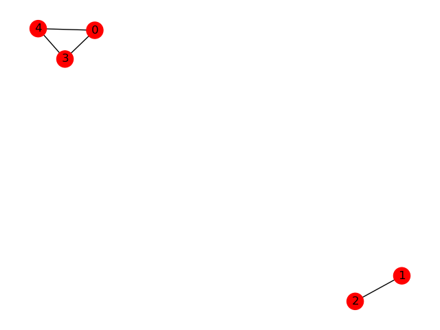
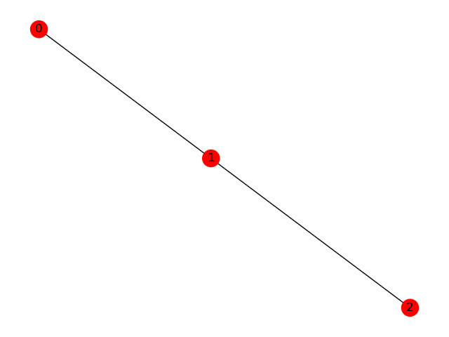
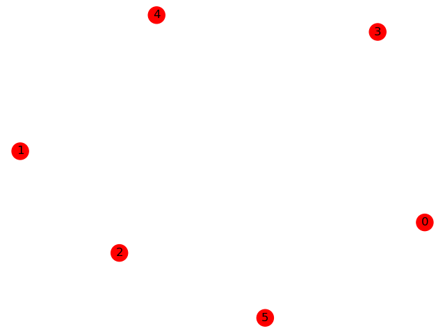
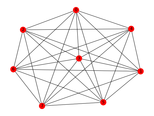
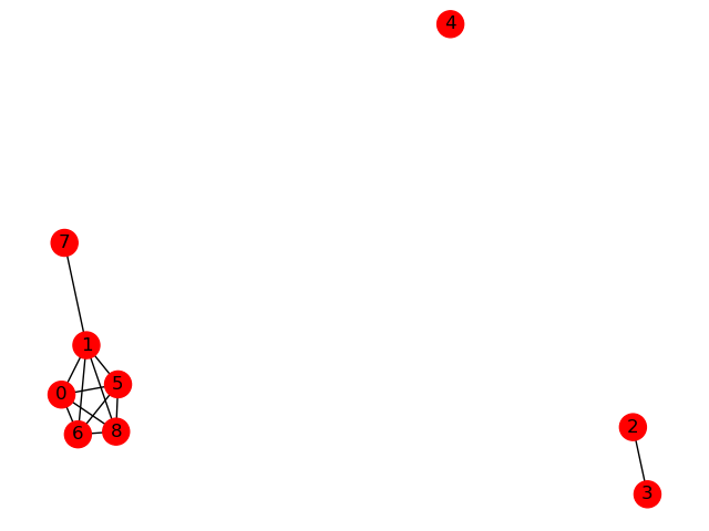
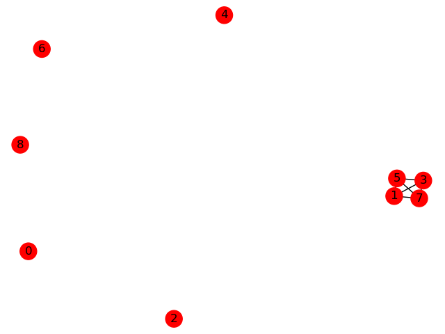
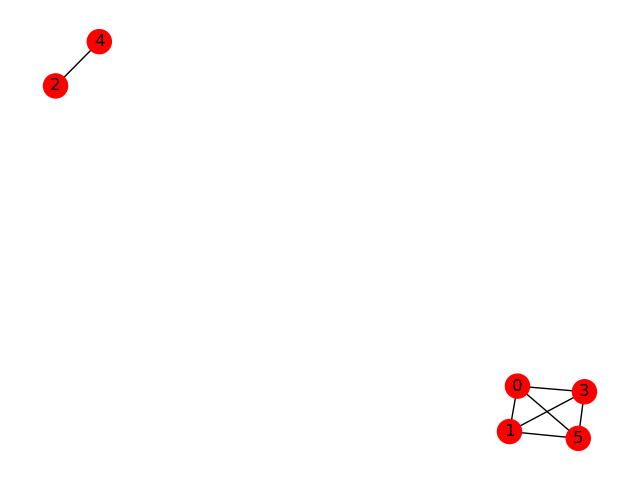
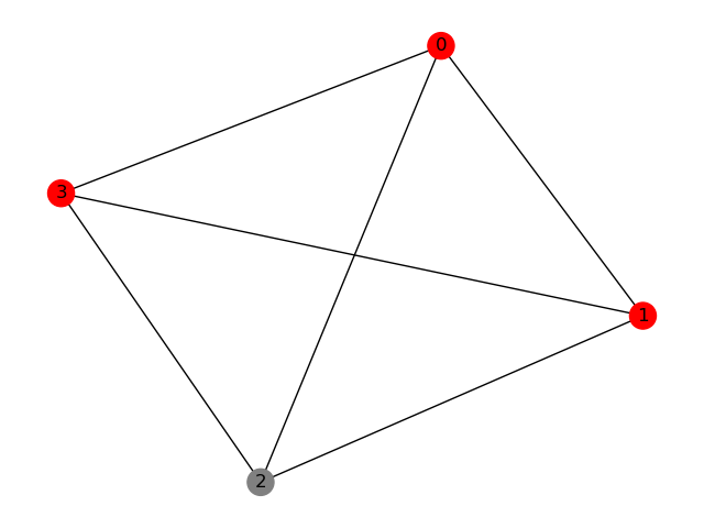
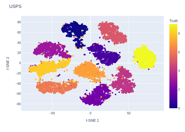
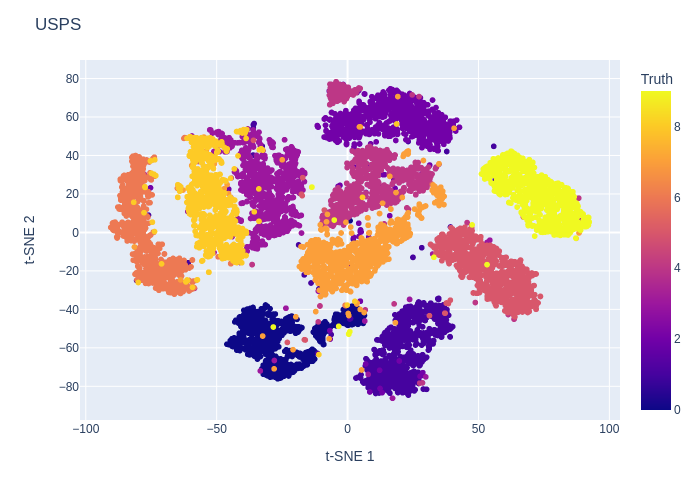


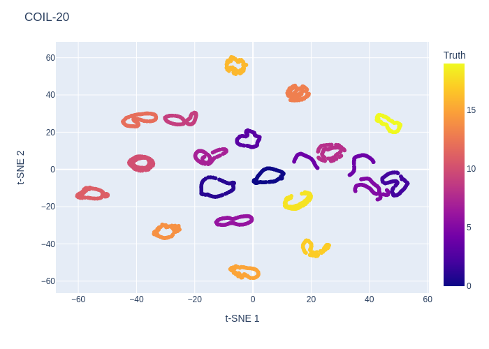


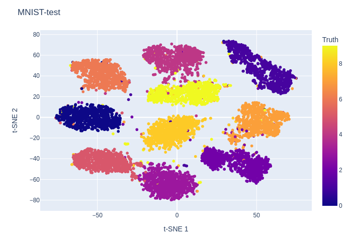
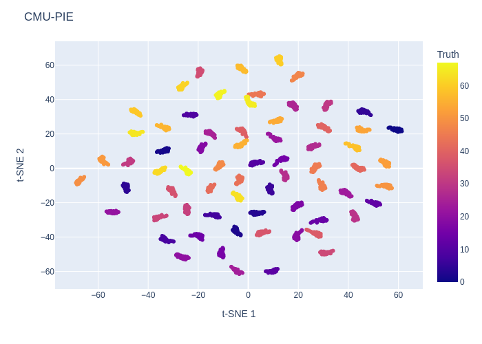

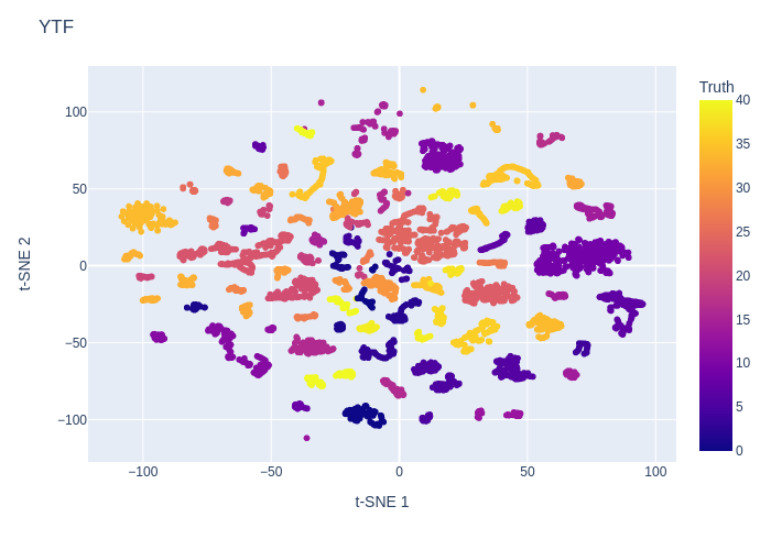

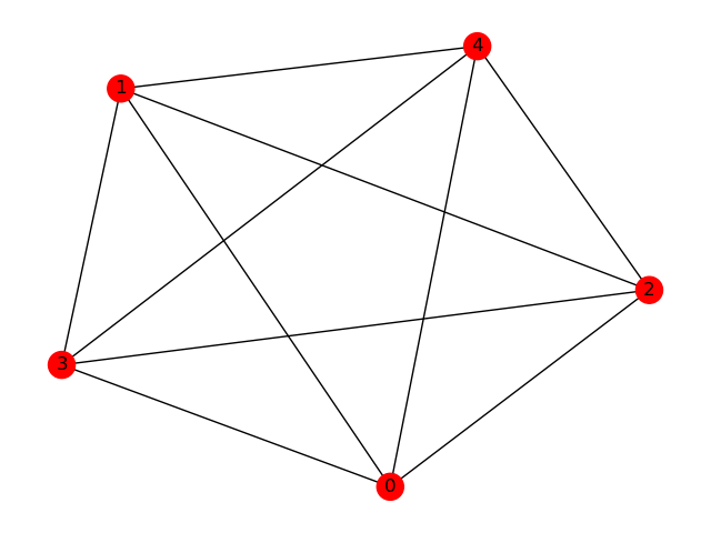
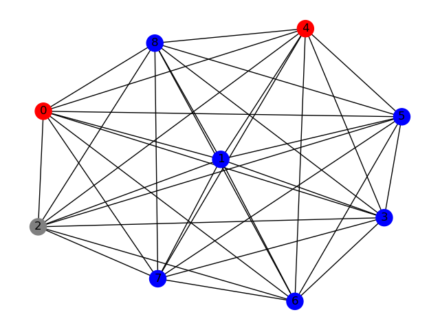
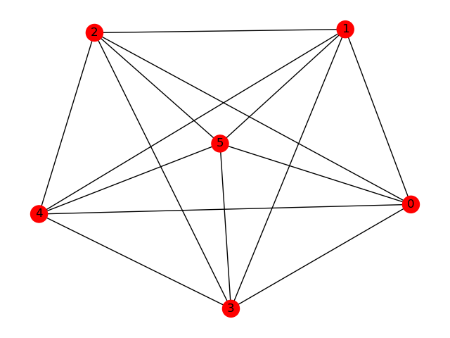
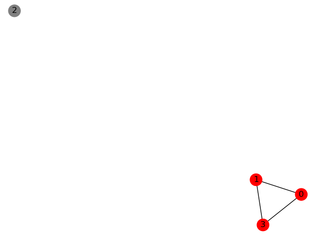

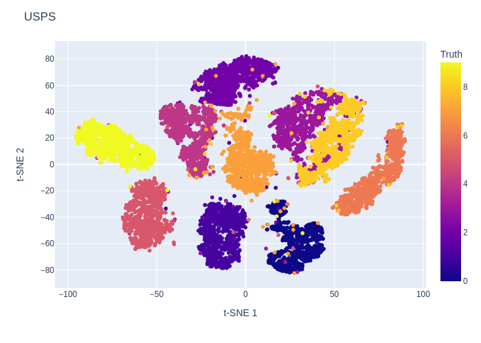
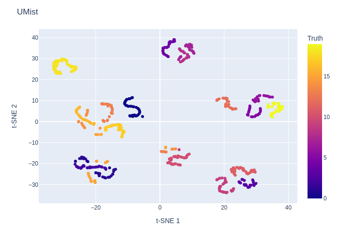
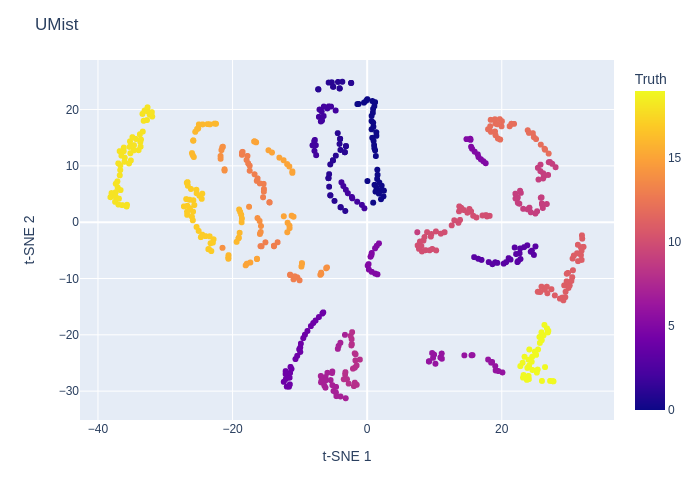

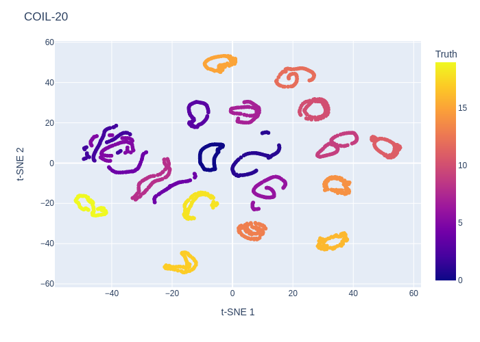

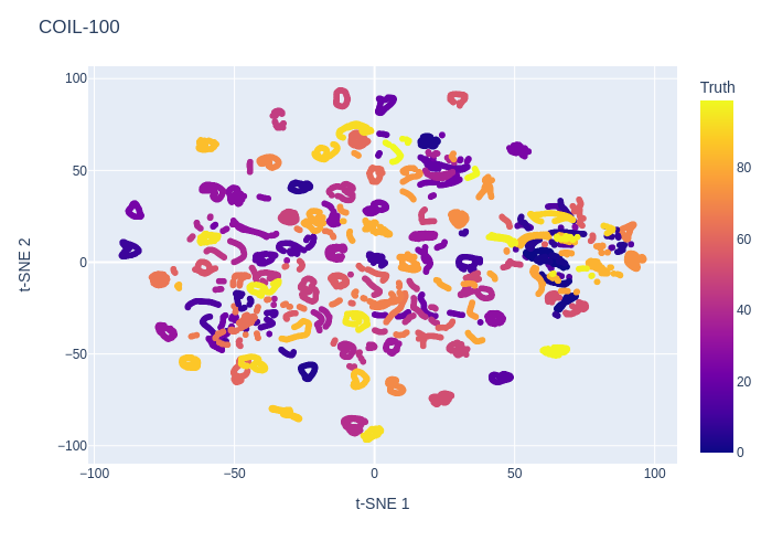
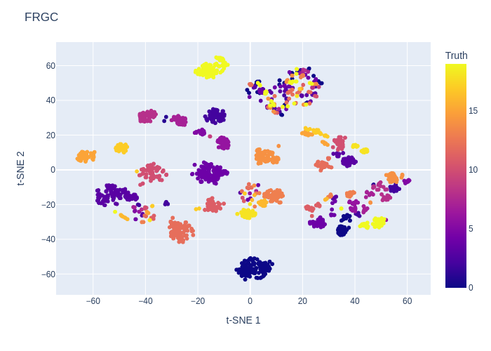
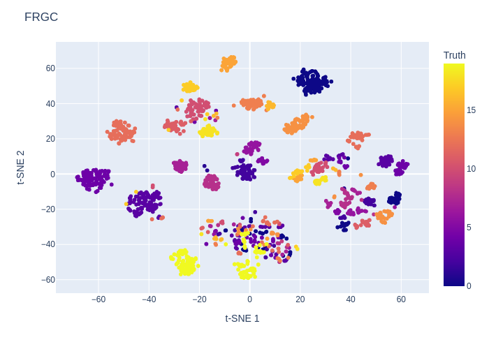
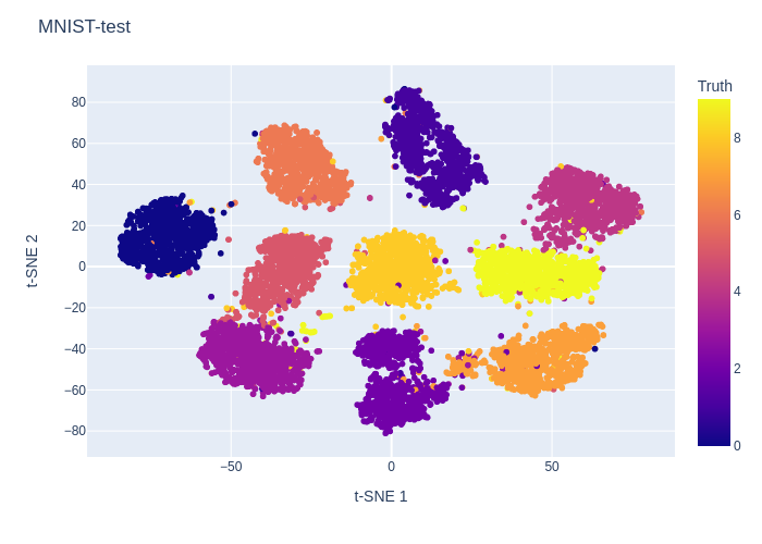
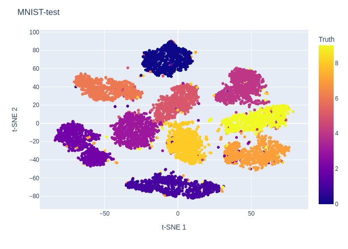
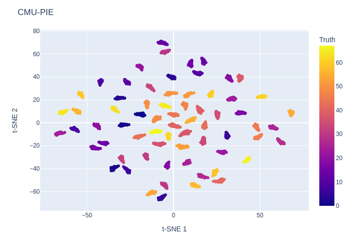
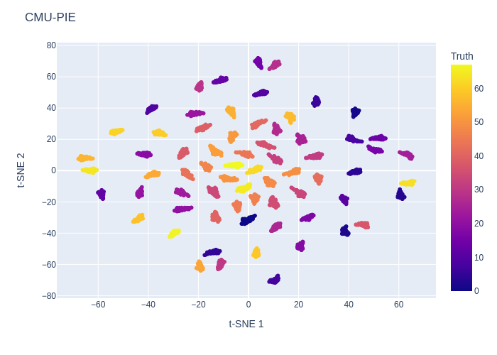

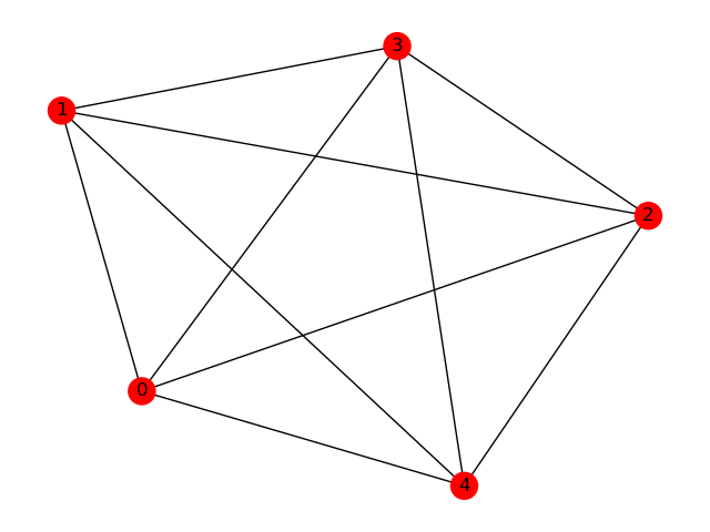
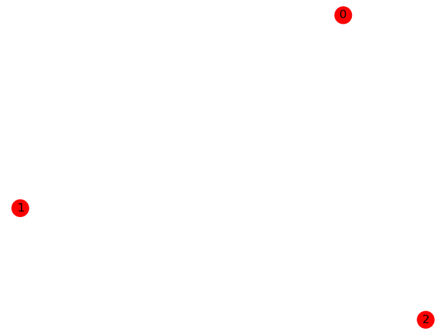

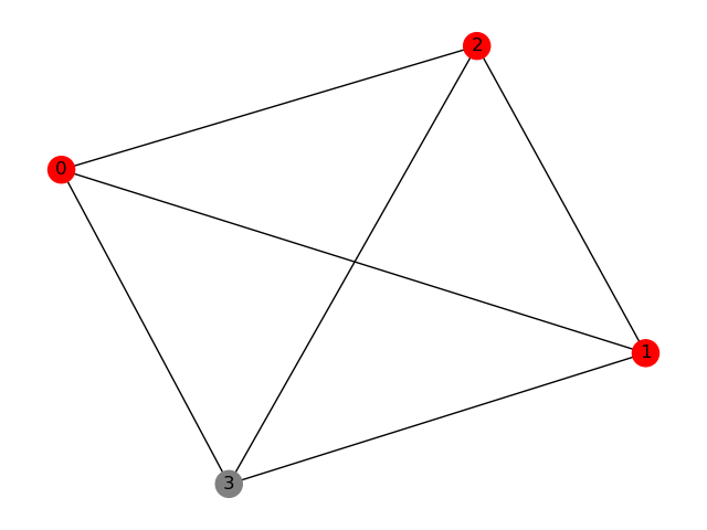
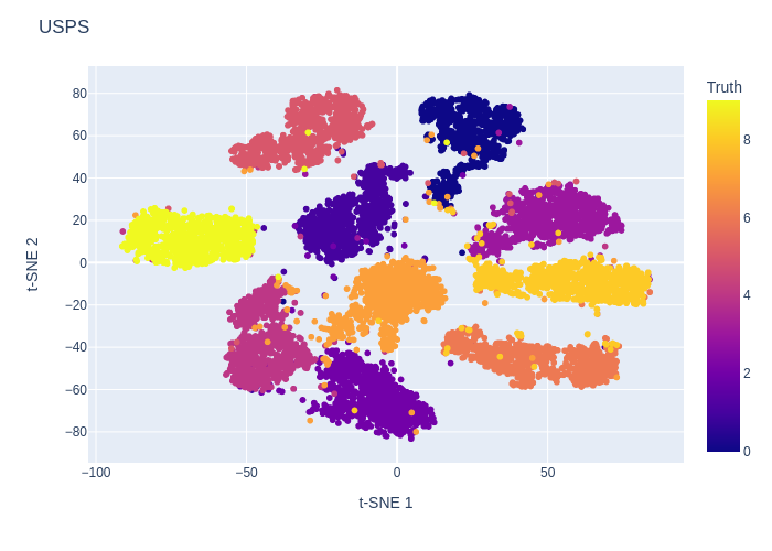


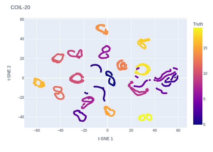
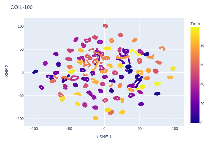
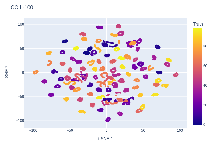


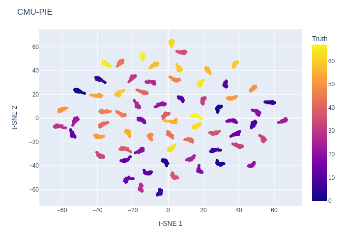


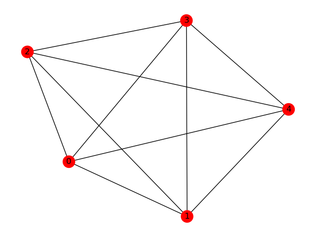
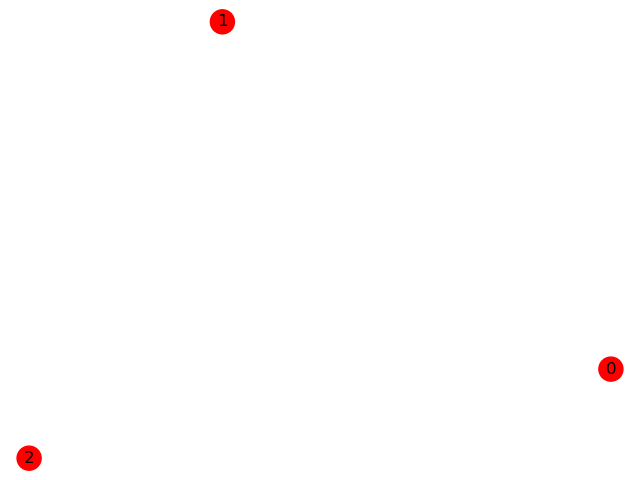
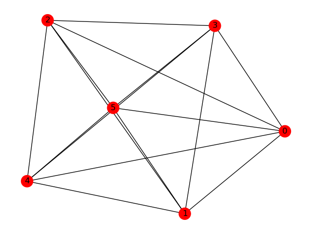
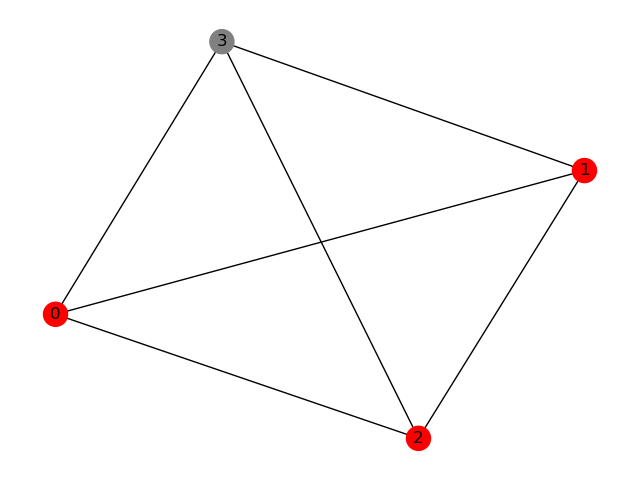


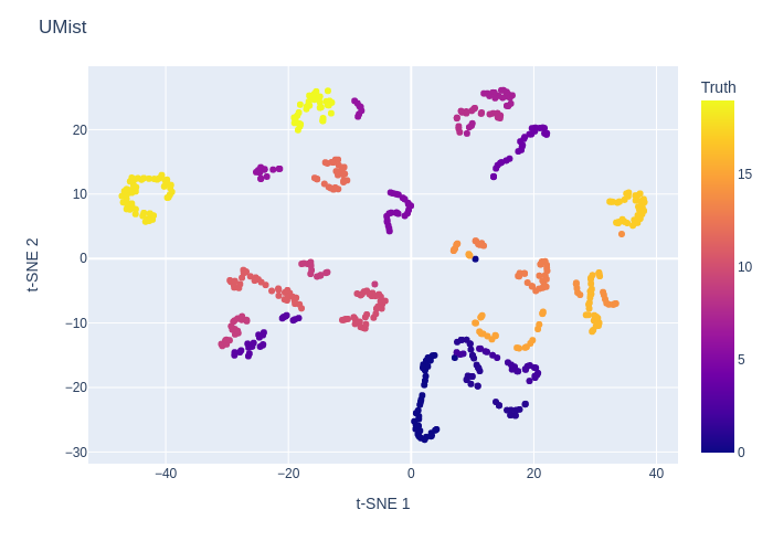


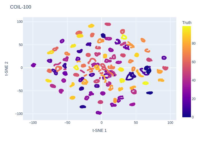
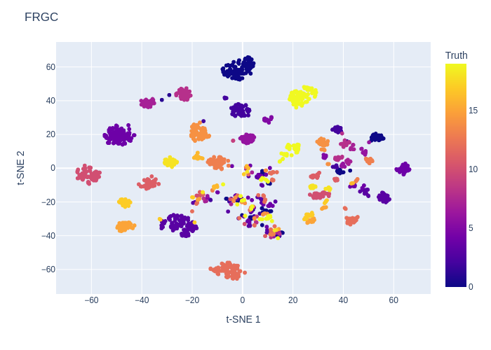


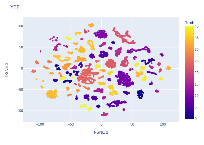
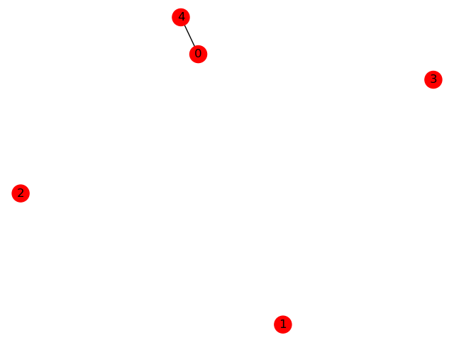
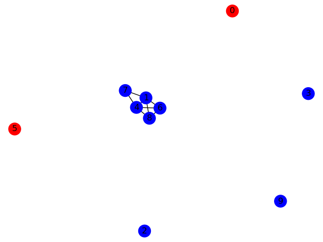
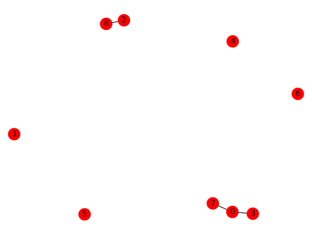
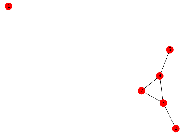
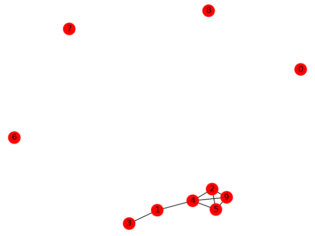
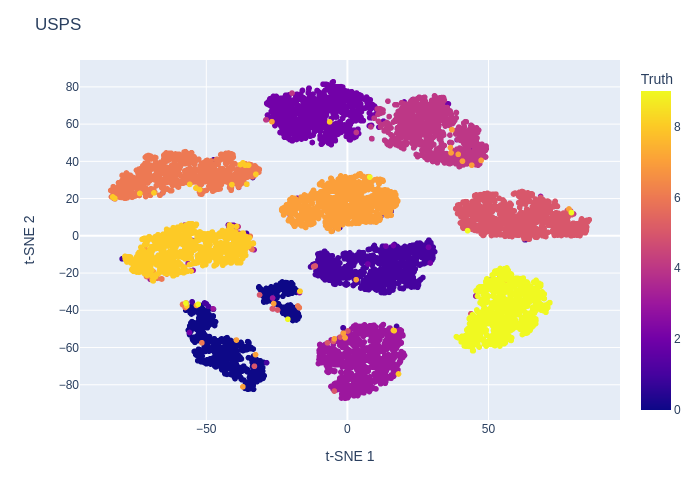


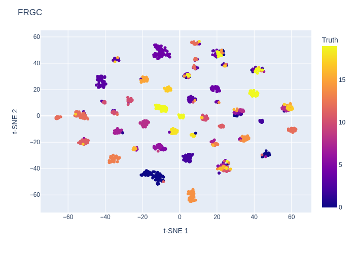
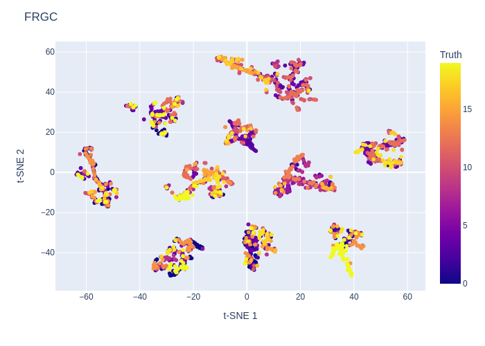

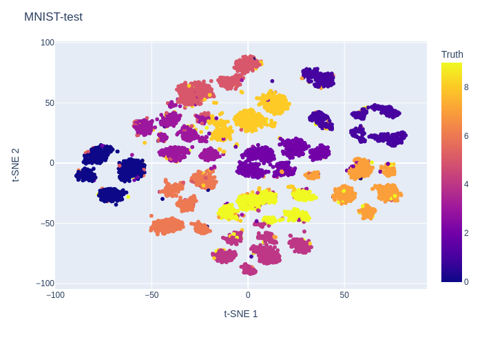
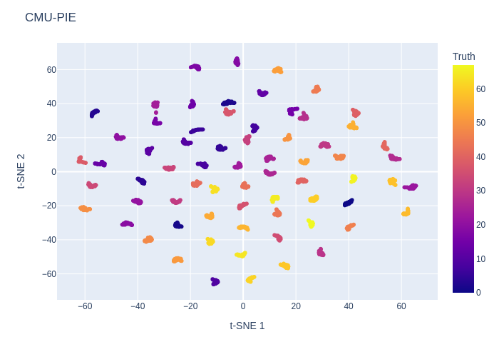
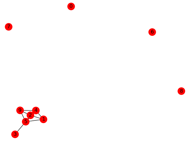
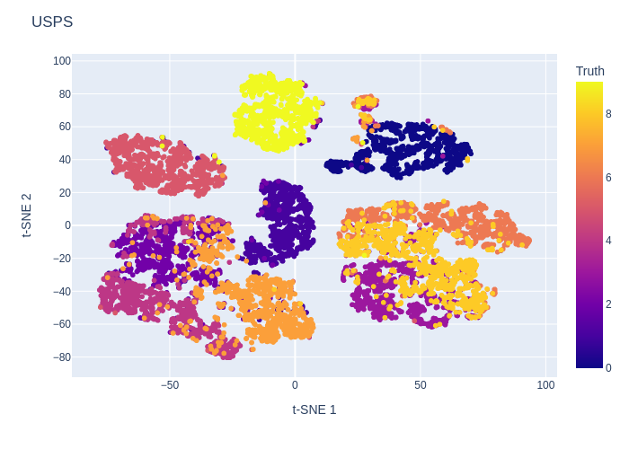

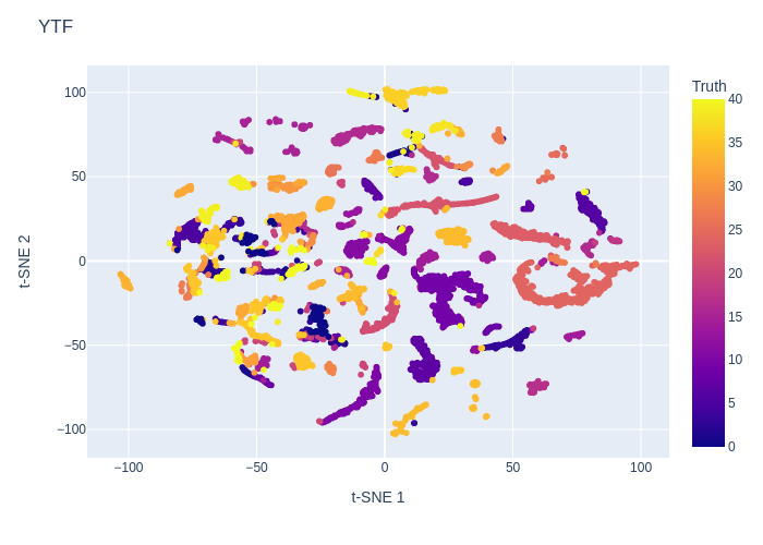


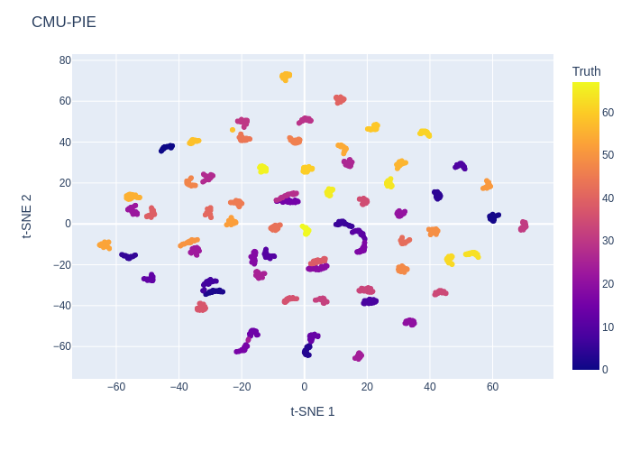
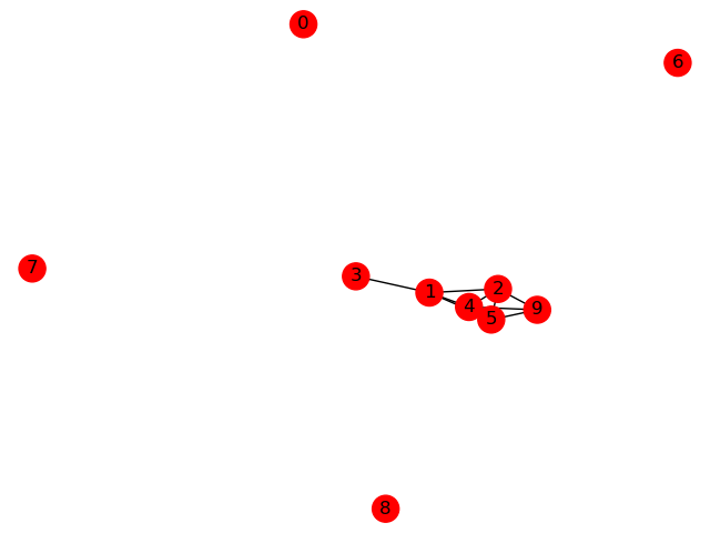


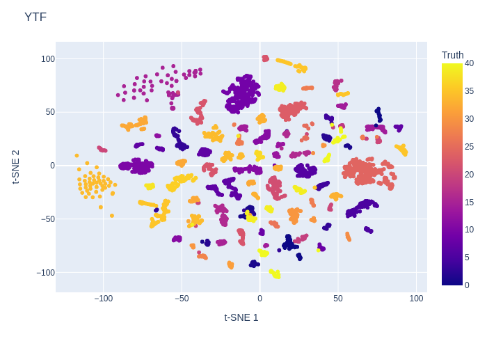

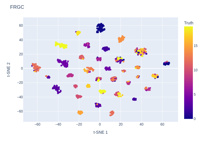


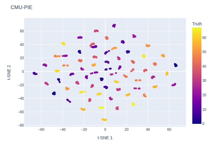
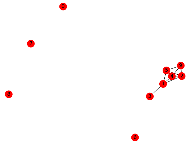

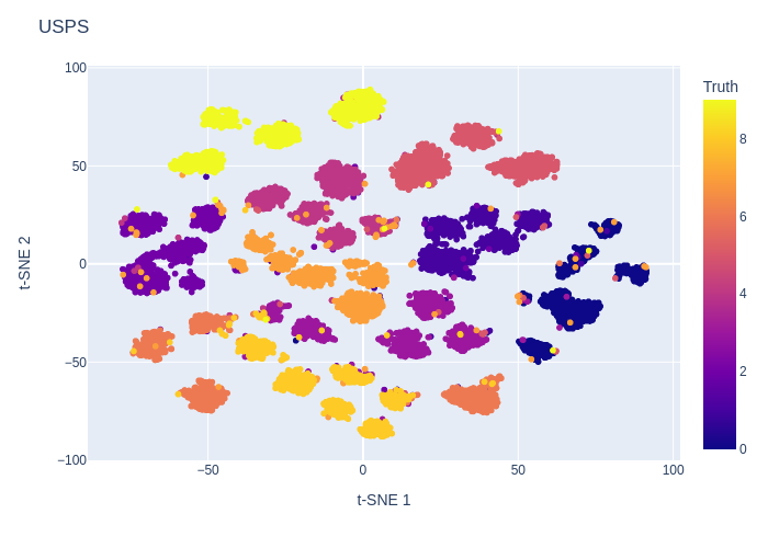

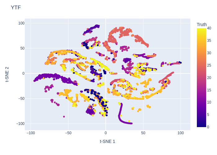
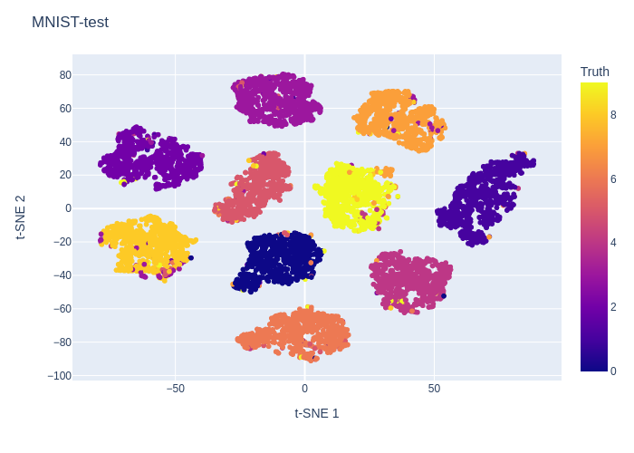
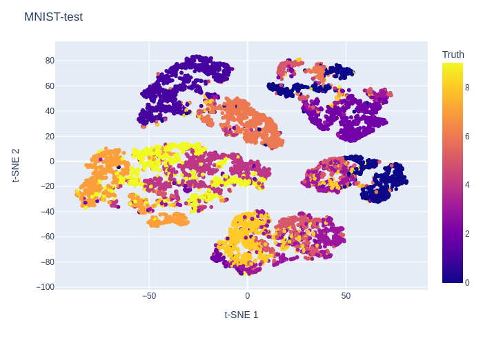

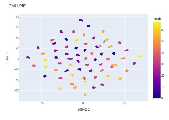
Selection of checkpoints
In this section, we present the results of the checkpoint selection experiment. We observe that all 20 obtained embedding spaces fail to reject the null hypothesis in the Dip test, as evident in the t-SNE visualizations displayed in Figure 35. (Each subfigure is annotated with the Dip test p-value). Despite this, indicating no significant departure from unimodality, we run the rest part of ACE on all 20 spaces as well as the score pooling algorithm for comparison. We present the rank correlation results with NMI and ACC, employing the Silhouette score, Calinski-Harabasz index, and Davies-Bouldin index, in Table 10. The pooled scores, compared with paired scores, show superior performance across all reported indices in Table 10. This underscores the unreliable nature of conventional paired scores for evaluation, emphasizing the importance of comparing and evaluating clustering results within the same space. In this experiment, pooled scores exhibit slightly better performance than ACE scores, a reasonable outcome considering the lack of significant multimodality in the spaces and our strategy aimed at selecting and ranking spaces based on differences in quality.
| Silhouette score (cosine) | Silhouette score (euclidean) | Davies-Bouldin index | Calinski-Harabasz index | |||||
| NMI | ||||||||
| Paired score | -0.75 | -0.59 | -0.74 | -0.57 | -0.79 | -0.64 | -0.82 | -0.68 |
| Pooled score | 0.43 | 0.34 | 0.43 | 0.34 | 0.29 | 0.21 | 0.52 | 0.42 |
| ACE | 0.40 | 0.29 | 0.40 | 0.29 | 0.39 | 0.25 | 0.52 | 0.37 |
| ACC | ||||||||
| Paired score | -0.75 | -0.58 | -0.74 | -0.56 | -0.80 | -0.66 | -0.82 | -0.69 |
| Pooled score | 0.43 | 0.32 | 0.43 | 0.32 | 0.28 | 0.19 | 0.52 | 0.40 |
| ACE | 0.40 | 0.28 | 0.40 | 0.28 | 0.40 | 0.25 | 0.52 | 0.37 |
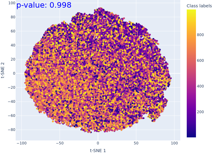
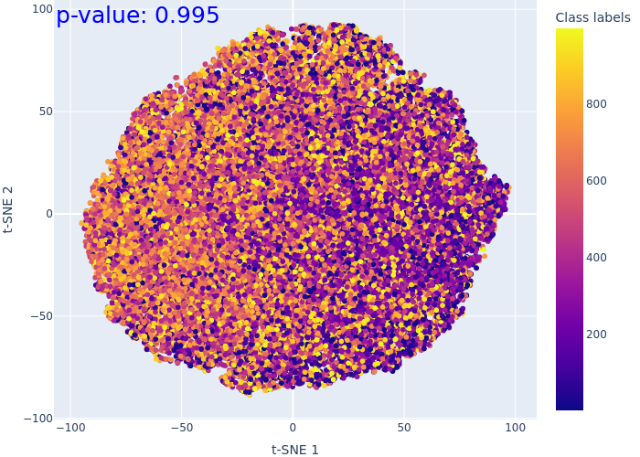
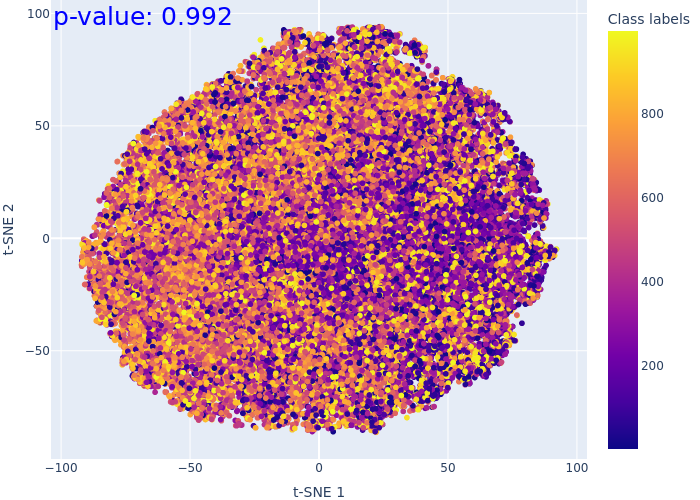
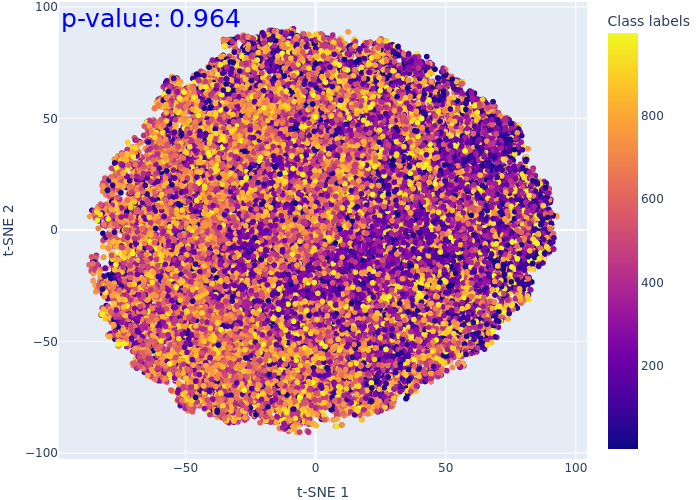
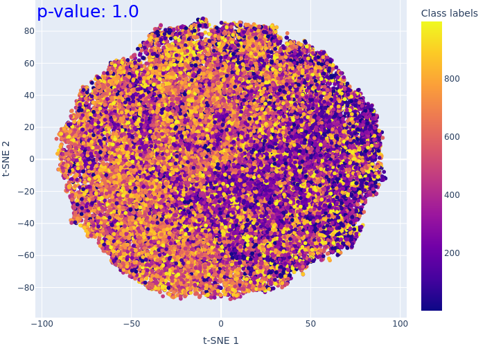

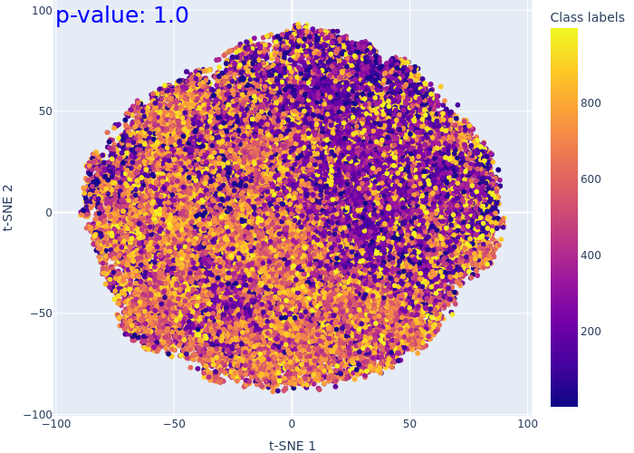
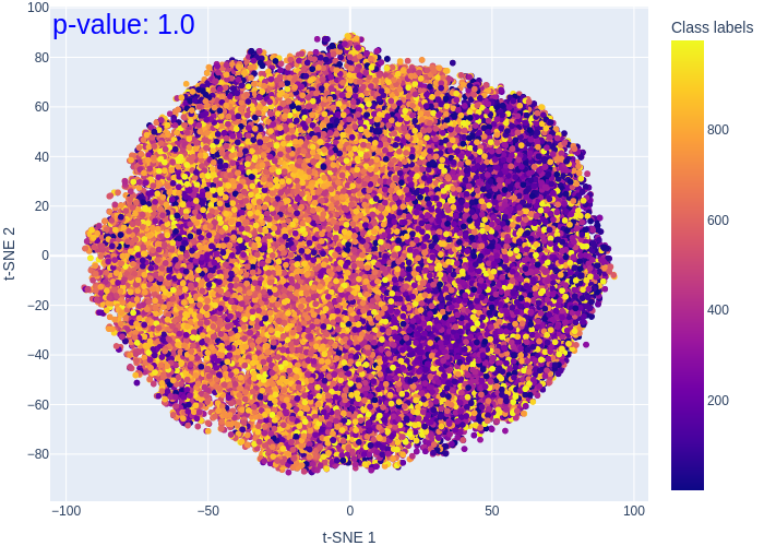
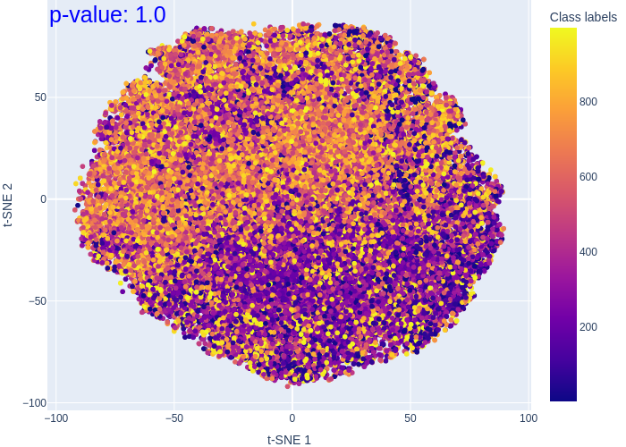
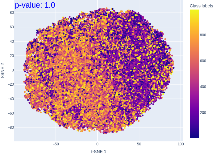
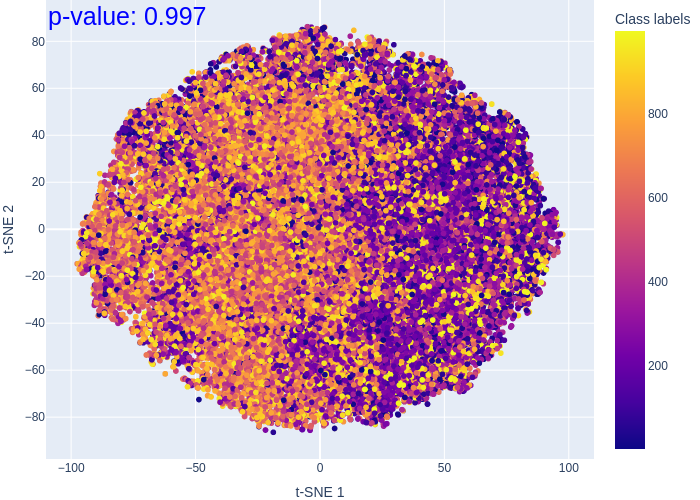
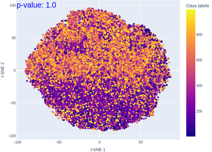
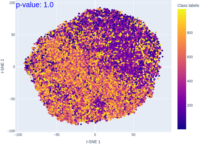
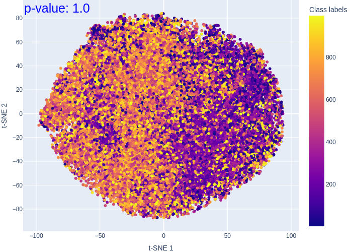
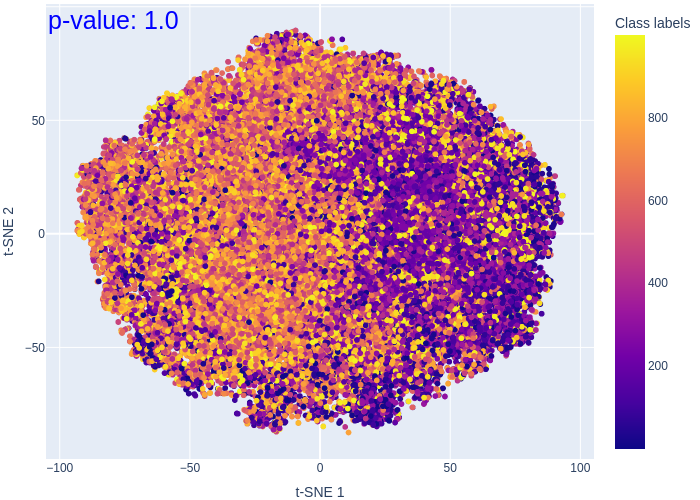
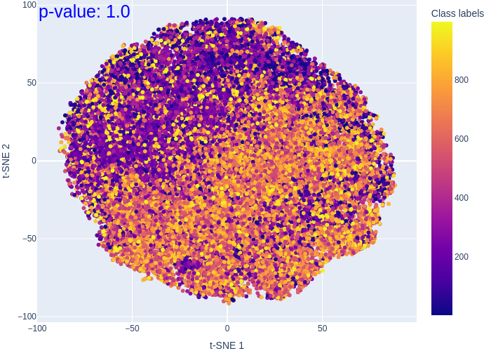
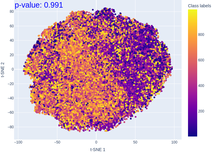
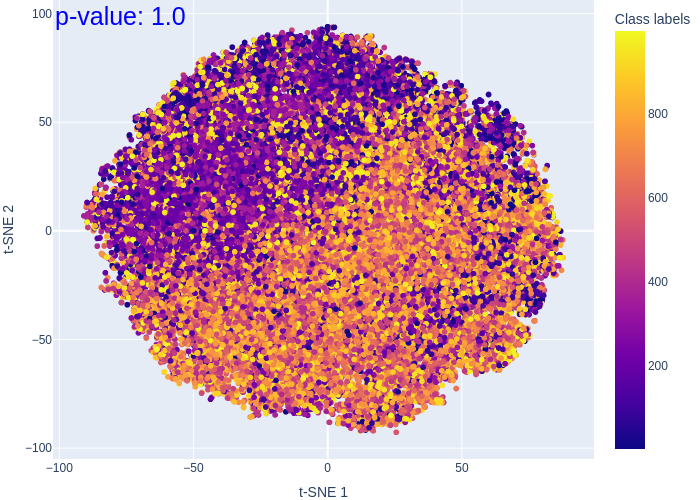
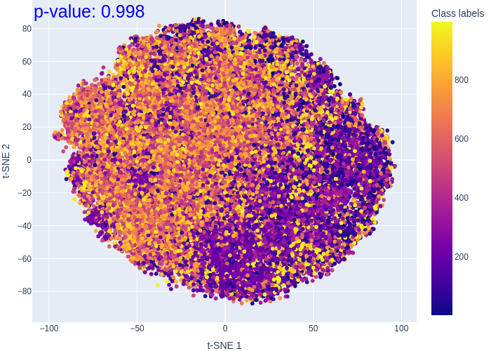
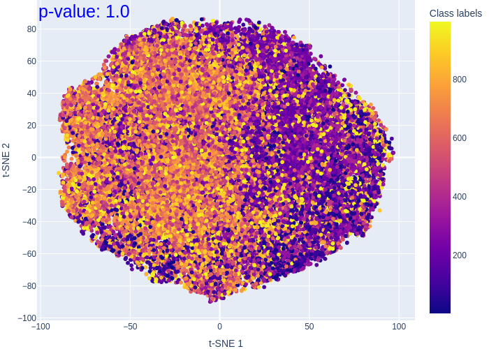
A.6.5 Ablation studies
In this section, we conduct a series of ablation studies and sensitivity analyses to examine the impact of various components or factors within our algorithm on the overall evaluation performance. Our ablation studies specifically explore the effects of performing the Dip test, employing different FWERs () for edge inclusion in link analysis, utilizing diverse link analysis algorithms, and applying different density-based algorithms. Additionally, we introduce a comparative study that includes the outlier space—an approach distinct from our existing strategy that excludes outlier space from clustering.
Dip Test
The Dip test serves as a filtering mechanism in our approach, targeting spaces that exhibit multimodality or clustering behavior. To assess the impact of removing the Dip test on model evaluation, specifically on the pooled score and ACE score, we conduct a thorough analysis. Tables 11 and 12 present a comparative evaluation, contrasting the performance of the pooled score with and without the Dip test, as well as ACE scores with and without the Dip test. The evaluation is based on both rank correlation with ACC and NMI, focusing on the hyperparameter tuning task. Similarly, Tables 13 and 14 extend this analysis to the task of determining the number of clusters. In our observations, we note that the application of the Dip test tends to enhance the performance of ACE in certain tasks, while its impact on the pooled score is relatively marginal. Specifically, ACE exhibits significant improvements (compared to ACE without the Dip test) in tasks such as hyperparameter tuning for JULE and DEPICT (Davies-Bouldin index). Additionally, notable improvements are observed in the task for determining the number of clusters for JULE (Davies-Bouldin index, Silhouette score using both euclidean and cosine distances) and DEPICT (Davies-Bouldin index, Silhouette score using euclidean distance). This observed enhancement in ACE performance can be attributed to its dependency on the quality of retained spaces. The proposed ACE relies on the retained spaces for voting and ranking, ultimately generating a quality score. In contrast, the pooled score simply averages over all retained spaces. In summary, our findings suggest that the Dip test contributes to the effectiveness of ACE in specific tasks, while its impact on the pooled score remains limited.
| USPS | YTF | FRGC | MNIST-test | CMU-PIE | UMist | COIL-20 | COIL-100 | Average | ||||||||||
| JULE: Calinski-Harabasz index | ||||||||||||||||||
| Paired score | 0.17 | 0.13 | 0.52 | 0.40 | -0.13 | -0.10 | 0.49 | 0.34 | -0.13 | -0.08 | 0.70 | 0.50 | 0.53 | 0.38 | 0.20 | 0.19 | 0.29 | 0.22 |
| Pooled score (w/o. Dip test) | 0.85 | 0.68 | 0.91 | 0.79 | 0.31 | 0.23 | 0.82 | 0.67 | 0.90 | 0.77 | 0.63 | 0.44 | 0.61 | 0.46 | 0.91 | 0.76 | 0.74 | 0.60 |
| Pooled score | 0.84 | 0.68 | 0.91 | 0.79 | 0.29 | 0.22 | 0.82 | 0.67 | 0.94 | 0.82 | 0.81 | 0.60 | 0.62 | 0.47 | 0.89 | 0.73 | 0.77 | 0.62 |
| ACE (w/o .Dip test) | 0.80 | 0.63 | 0.90 | 0.73 | 0.42 | 0.30 | 0.86 | 0.70 | 0.98 | 0.93 | 0.71 | 0.51 | 0.92 | 0.76 | 0.92 | 0.79 | 0.81 | 0.67 |
| ACE | 0.80 | 0.63 | 0.90 | 0.73 | 0.39 | 0.26 | 0.87 | 0.71 | 0.98 | 0.90 | 0.81 | 0.61 | 0.60 | 0.45 | 0.95 | 0.82 | 0.79 | 0.64 |
| JULE: Davies-Bouldin index | ||||||||||||||||||
| Paired score | -0.10 | -0.03 | -0.32 | -0.21 | -0.08 | -0.05 | -0.13 | -0.06 | 0.26 | 0.20 | 0.62 | 0.44 | 0.61 | 0.42 | 0.43 | 0.35 | 0.16 | 0.13 |
| Pooled score (w/o. Dip test) | -0.26 | -0.13 | -0.46 | -0.34 | 0.12 | 0.08 | -0.15 | -0.06 | 0.92 | 0.78 | -0.35 | -0.24 | -0.24 | -0.17 | -0.46 | -0.35 | -0.11 | -0.05 |
| Pooled score | -0.26 | -0.12 | -0.46 | -0.34 | 0.11 | 0.07 | -0.16 | -0.07 | 0.92 | 0.78 | 0.30 | 0.20 | -0.25 | -0.17 | -0.46 | -0.35 | -0.03 | -0.00 |
| ACE (w/o .Dip test) | -0.08 | -0.02 | -0.30 | -0.21 | 0.22 | 0.16 | 0.73 | 0.55 | 0.03 | -0.01 | 0.74 | 0.54 | 0.29 | 0.26 | -0.49 | -0.39 | 0.14 | 0.11 |
| ACE | -0.08 | -0.02 | -0.30 | -0.21 | 0.22 | 0.16 | 0.73 | 0.55 | 0.10 | 0.06 | 0.38 | 0.27 | 0.23 | 0.22 | 0.48 | 0.33 | 0.22 | 0.17 |
| JULE: Silhouette score (cosine distance) | ||||||||||||||||||
| Paired score | 0.28 | 0.22 | 0.73 | 0.56 | 0.09 | 0.06 | 0.63 | 0.47 | 0.50 | 0.36 | 0.71 | 0.50 | 0.68 | 0.50 | 0.74 | 0.54 | 0.54 | 0.40 |
| Pooled score (w/o. Dip test) | 0.71 | 0.58 | 0.93 | 0.81 | 0.41 | 0.28 | 0.79 | 0.64 | 0.95 | 0.84 | 0.58 | 0.39 | 0.26 | 0.16 | 0.69 | 0.53 | 0.66 | 0.53 |
| Pooled score | 0.70 | 0.56 | 0.93 | 0.81 | 0.40 | 0.27 | 0.79 | 0.64 | 0.95 | 0.85 | 0.77 | 0.56 | 0.27 | 0.16 | 0.68 | 0.52 | 0.69 | 0.55 |
| ACE (w/o .Dip test) | 0.89 | 0.73 | 0.93 | 0.83 | 0.52 | 0.35 | 0.81 | 0.66 | 0.99 | 0.94 | 0.83 | 0.65 | 0.44 | 0.38 | 0.91 | 0.77 | 0.79 | 0.66 |
| ACE | 0.89 | 0.73 | 0.93 | 0.83 | 0.52 | 0.35 | 0.81 | 0.66 | 0.99 | 0.93 | 0.79 | 0.59 | 0.44 | 0.38 | 0.92 | 0.78 | 0.79 | 0.66 |
| JULE: Silhouette score (euclidean distance) | ||||||||||||||||||
| Paired score | 0.27 | 0.20 | 0.72 | 0.55 | 0.04 | 0.03 | 0.56 | 0.41 | 0.42 | 0.30 | 0.70 | 0.50 | 0.64 | 0.46 | 0.55 | 0.41 | 0.49 | 0.36 |
| Pooled score (w/o. Dip test) | 0.70 | 0.57 | 0.90 | 0.77 | 0.41 | 0.28 | 0.78 | 0.63 | 0.95 | 0.84 | 0.64 | 0.43 | 0.25 | 0.16 | 0.71 | 0.54 | 0.67 | 0.53 |
| Pooled score | 0.71 | 0.58 | 0.90 | 0.77 | 0.41 | 0.28 | 0.78 | 0.63 | 0.96 | 0.85 | 0.79 | 0.57 | 0.26 | 0.16 | 0.70 | 0.54 | 0.69 | 0.55 |
| ACE (w/o .Dip test) | 0.88 | 0.72 | 0.89 | 0.75 | 0.42 | 0.28 | 0.81 | 0.65 | 0.98 | 0.92 | 0.88 | 0.70 | 0.41 | 0.36 | 0.91 | 0.78 | 0.77 | 0.65 |
| ACE | 0.88 | 0.72 | 0.89 | 0.75 | 0.42 | 0.28 | 0.81 | 0.65 | 0.98 | 0.90 | 0.88 | 0.70 | 0.41 | 0.36 | 0.92 | 0.78 | 0.77 | 0.64 |
| DEPICT: Calinski-Harabasz index | ||||||||||||||||||
| Paired score | 0.76 | 0.57 | 0.44 | 0.26 | 0.76 | 0.57 | 0.89 | 0.72 | 0.49 | 0.44 | 0.67 | 0.51 | ||||||
| Pooled score (w/o. Dip test) | 0.96 | 0.84 | 0.53 | 0.41 | 0.90 | 0.77 | 0.96 | 0.87 | 0.73 | 0.59 | 0.82 | 0.70 | ||||||
| Pooled score | 0.96 | 0.83 | 0.53 | 0.41 | 0.90 | 0.77 | 0.96 | 0.87 | 0.61 | 0.56 | 0.79 | 0.69 | ||||||
| ACE (w/o .Dip test) | 0.91 | 0.77 | 0.56 | 0.44 | 0.94 | 0.82 | 0.96 | 0.87 | 0.96 | 0.88 | 0.87 | 0.75 | ||||||
| ACE | 0.91 | 0.77 | 0.56 | 0.44 | 0.94 | 0.82 | 0.96 | 0.87 | 0.96 | 0.87 | 0.87 | 0.75 | ||||||
| DEPICT: Davies-Bouldin index | ||||||||||||||||||
| Paired score | 0.81 | 0.59 | 0.45 | 0.31 | 0.90 | 0.74 | 0.89 | 0.72 | 0.63 | 0.59 | 0.73 | 0.59 | ||||||
| Pooled score (w/o. Dip test) | 0.95 | 0.84 | 0.49 | 0.35 | 0.65 | 0.50 | 0.50 | 0.36 | 0.23 | 0.06 | 0.56 | 0.42 | ||||||
| Pooled score | 0.96 | 0.88 | 0.49 | 0.35 | 0.64 | 0.48 | 0.43 | 0.32 | -0.77 | -0.61 | 0.35 | 0.28 | ||||||
| ACE (w/o .Dip test) | 0.90 | 0.79 | 0.76 | 0.58 | 0.91 | 0.79 | 0.95 | 0.83 | 0.63 | 0.49 | 0.83 | 0.70 | ||||||
| ACE | 0.91 | 0.82 | 0.76 | 0.58 | 0.91 | 0.79 | 0.96 | 0.87 | 0.98 | 0.92 | 0.90 | 0.80 | ||||||
| DEPICT: Silhouette score (cosine distance) | ||||||||||||||||||
| Paired score | 0.81 | 0.62 | 0.45 | 0.33 | 0.90 | 0.75 | 0.89 | 0.72 | 0.77 | 0.58 | 0.76 | 0.60 | ||||||
| Pooled score (w/o. Dip test) | 0.96 | 0.83 | 0.68 | 0.56 | 0.94 | 0.82 | 0.95 | 0.87 | 0.95 | 0.86 | 0.90 | 0.79 | ||||||
| Pooled score | 0.96 | 0.86 | 0.68 | 0.56 | 0.94 | 0.82 | 0.97 | 0.90 | 0.93 | 0.79 | 0.90 | 0.78 | ||||||
| ACE (w/o .Dip test) | 0.97 | 0.90 | 0.71 | 0.56 | 0.94 | 0.82 | 0.98 | 0.91 | 0.95 | 0.84 | 0.91 | 0.80 | ||||||
| ACE | 0.97 | 0.90 | 0.71 | 0.56 | 0.94 | 0.82 | 0.97 | 0.90 | 0.94 | 0.83 | 0.91 | 0.80 | ||||||
| DEPICT: Silhouette score (euclidean distance) | ||||||||||||||||||
| Paired score | 0.73 | 0.50 | 0.47 | 0.36 | 0.79 | 0.65 | 0.86 | 0.69 | 0.59 | 0.52 | 0.69 | 0.54 | ||||||
| Pooled score (w/o. Dip test) | 0.96 | 0.84 | 0.65 | 0.53 | 0.94 | 0.82 | 0.97 | 0.90 | 0.95 | 0.86 | 0.89 | 0.79 | ||||||
| Pooled score | 0.96 | 0.86 | 0.65 | 0.53 | 0.94 | 0.82 | 0.97 | 0.90 | 0.92 | 0.75 | 0.89 | 0.77 | ||||||
| ACE (w/o .Dip test) | 0.92 | 0.80 | 0.65 | 0.50 | 0.95 | 0.83 | 0.98 | 0.90 | 0.95 | 0.83 | 0.89 | 0.77 | ||||||
| ACE | 0.97 | 0.88 | 0.65 | 0.50 | 0.95 | 0.83 | 0.98 | 0.90 | 0.94 | 0.82 | 0.90 | 0.79 | ||||||
| USPS | YTF | FRGC | MNIST-test | CMU-PIE | UMist | COIL-20 | COIL-100 | Average | ||||||||||
| JULE: Calinski-Harabasz index | ||||||||||||||||||
| Paired score | 0.04 | 0.05 | 0.39 | 0.27 | -0.26 | -0.18 | 0.31 | 0.21 | -0.20 | -0.12 | 0.64 | 0.45 | 0.57 | 0.40 | 0.09 | 0.08 | 0.20 | 0.14 |
| Pooled score (w/o. Dip test) | 0.92 | 0.79 | 0.78 | 0.61 | 0.30 | 0.21 | 0.91 | 0.77 | 0.91 | 0.78 | 0.65 | 0.47 | 0.57 | 0.42 | 0.91 | 0.78 | 0.74 | 0.60 |
| Pooled score | 0.91 | 0.78 | 0.78 | 0.61 | 0.30 | 0.21 | 0.91 | 0.77 | 0.95 | 0.83 | 0.81 | 0.60 | 0.58 | 0.43 | 0.90 | 0.75 | 0.77 | 0.62 |
| ACE (w/o .Dip test) | 0.90 | 0.77 | 0.73 | 0.54 | 0.59 | 0.44 | 0.95 | 0.81 | 0.97 | 0.89 | 0.67 | 0.49 | 0.89 | 0.72 | 0.88 | 0.74 | 0.82 | 0.68 |
| ACE | 0.90 | 0.77 | 0.73 | 0.54 | 0.49 | 0.36 | 0.95 | 0.82 | 0.97 | 0.87 | 0.81 | 0.61 | 0.57 | 0.40 | 0.93 | 0.81 | 0.79 | 0.65 |
| JULE: Davies-Bouldin index | ||||||||||||||||||
| Paired score | -0.27 | -0.15 | -0.14 | -0.09 | -0.23 | -0.14 | -0.35 | -0.19 | 0.20 | 0.16 | 0.53 | 0.36 | 0.63 | 0.44 | 0.33 | 0.26 | 0.09 | 0.08 |
| Pooled score (w/o. Dip test) | -0.49 | -0.21 | -0.35 | -0.23 | 0.49 | 0.36 | -0.35 | -0.20 | 0.89 | 0.76 | -0.47 | -0.34 | -0.30 | -0.22 | -0.48 | -0.34 | -0.13 | -0.05 |
| Pooled score | -0.49 | -0.20 | -0.35 | -0.23 | 0.48 | 0.36 | -0.35 | -0.21 | 0.89 | 0.75 | 0.17 | 0.11 | -0.29 | -0.22 | -0.48 | -0.34 | -0.05 | 0.00 |
| ACE (w/o .Dip test) | -0.30 | -0.09 | -0.07 | -0.07 | 0.53 | 0.38 | 0.79 | 0.64 | 0.01 | -0.04 | 0.66 | 0.45 | 0.27 | 0.23 | -0.49 | -0.35 | 0.17 | 0.14 |
| ACE | -0.30 | -0.09 | -0.07 | -0.07 | 0.53 | 0.38 | 0.79 | 0.64 | 0.07 | 0.03 | 0.27 | 0.20 | 0.21 | 0.18 | 0.44 | 0.28 | 0.24 | 0.19 |
| JULE: Silhouette score (cosine distance) | ||||||||||||||||||
| Paired score | 0.17 | 0.14 | 0.59 | 0.41 | 0.07 | 0.06 | 0.47 | 0.33 | 0.45 | 0.33 | 0.64 | 0.46 | 0.70 | 0.51 | 0.64 | 0.45 | 0.47 | 0.34 |
| Pooled score (w/o. Dip test) | 0.75 | 0.70 | 0.73 | 0.55 | 0.71 | 0.53 | 0.90 | 0.73 | 0.96 | 0.87 | 0.57 | 0.38 | 0.19 | 0.10 | 0.60 | 0.44 | 0.68 | 0.54 |
| Pooled score | 0.74 | 0.68 | 0.73 | 0.55 | 0.71 | 0.53 | 0.90 | 0.73 | 0.96 | 0.88 | 0.75 | 0.55 | 0.20 | 0.11 | 0.61 | 0.44 | 0.70 | 0.56 |
| ACE (w/o .Dip test) | 0.96 | 0.85 | 0.74 | 0.55 | 0.82 | 0.65 | 0.92 | 0.78 | 0.99 | 0.94 | 0.80 | 0.61 | 0.41 | 0.32 | 0.81 | 0.65 | 0.81 | 0.67 |
| ACE | 0.96 | 0.85 | 0.74 | 0.55 | 0.82 | 0.65 | 0.92 | 0.78 | 0.98 | 0.92 | 0.78 | 0.58 | 0.41 | 0.32 | 0.84 | 0.68 | 0.81 | 0.67 |
| JULE: Silhouette score (euclidean distance) | ||||||||||||||||||
| Paired score | 0.14 | 0.12 | 0.54 | 0.39 | -0.08 | -0.02 | 0.41 | 0.27 | 0.36 | 0.27 | 0.64 | 0.46 | 0.67 | 0.48 | 0.44 | 0.31 | 0.39 | 0.28 |
| Pooled score (w/o. Dip test) | 0.74 | 0.68 | 0.66 | 0.49 | 0.71 | 0.53 | 0.89 | 0.72 | 0.96 | 0.87 | 0.64 | 0.43 | 0.19 | 0.10 | 0.62 | 0.45 | 0.68 | 0.53 |
| Pooled score | 0.73 | 0.67 | 0.66 | 0.49 | 0.70 | 0.53 | 0.89 | 0.72 | 0.97 | 0.88 | 0.77 | 0.57 | 0.20 | 0.11 | 0.62 | 0.45 | 0.69 | 0.55 |
| ACE (w/o .Dip test) | 0.93 | 0.78 | 0.63 | 0.48 | 0.71 | 0.53 | 0.92 | 0.78 | 0.99 | 0.94 | 0.86 | 0.68 | 0.39 | 0.30 | 0.81 | 0.66 | 0.78 | 0.64 |
| ACE | 0.93 | 0.78 | 0.63 | 0.48 | 0.71 | 0.53 | 0.92 | 0.78 | 0.98 | 0.91 | 0.86 | 0.68 | 0.39 | 0.30 | 0.84 | 0.68 | 0.78 | 0.64 |
| DEPICT: Calinski-Harabasz index | ||||||||||||||||||
| Paired score | 0.56 | 0.40 | 0.54 | 0.35 | 0.76 | 0.57 | 0.88 | 0.69 | 0.48 | 0.43 | 0.64 | 0.49 | ||||||
| Pooled score (w/o. Dip test) | 0.94 | 0.83 | 0.54 | 0.45 | 0.92 | 0.79 | 0.95 | 0.86 | 0.74 | 0.62 | 0.82 | 0.71 | ||||||
| Pooled score | 0.94 | 0.82 | 0.54 | 0.45 | 0.92 | 0.79 | 0.95 | 0.86 | 0.62 | 0.55 | 0.79 | 0.69 | ||||||
| ACE (w/o .Dip test) | 0.82 | 0.72 | 0.61 | 0.45 | 0.91 | 0.82 | 0.97 | 0.91 | 0.98 | 0.91 | 0.86 | 0.76 | ||||||
| ACE | 0.82 | 0.72 | 0.61 | 0.45 | 0.91 | 0.82 | 0.97 | 0.91 | 0.96 | 0.87 | 0.86 | 0.75 | ||||||
| DEPICT: Davies-Bouldin index | ||||||||||||||||||
| Paired score | 0.61 | 0.42 | 0.48 | 0.32 | 0.92 | 0.74 | 0.88 | 0.69 | 0.62 | 0.56 | 0.70 | 0.55 | ||||||
| Pooled score (w/o. Dip test) | 0.93 | 0.80 | 0.40 | 0.28 | 0.65 | 0.50 | 0.45 | 0.32 | 0.24 | 0.07 | 0.53 | 0.39 | ||||||
| Pooled score | 0.95 | 0.84 | 0.40 | 0.28 | 0.64 | 0.48 | 0.38 | 0.28 | -0.76 | -0.60 | 0.32 | 0.26 | ||||||
| ACE (w/o .Dip test) | 0.99 | 0.96 | 0.65 | 0.46 | 0.90 | 0.74 | 0.99 | 0.92 | 0.60 | 0.46 | 0.82 | 0.71 | ||||||
| ACE | 0.99 | 0.96 | 0.65 | 0.46 | 0.90 | 0.74 | 0.99 | 0.96 | 0.96 | 0.87 | 0.90 | 0.80 | ||||||
| DEPICT: Silhouette score (cosine distance) | ||||||||||||||||||
| Paired score | 0.62 | 0.45 | 0.53 | 0.42 | 0.91 | 0.75 | 0.88 | 0.69 | 0.77 | 0.58 | 0.74 | 0.58 | ||||||
| Pooled score (w/o. Dip test) | 0.96 | 0.87 | 0.75 | 0.59 | 0.94 | 0.82 | 0.96 | 0.88 | 0.95 | 0.85 | 0.91 | 0.80 | ||||||
| Pooled score | 0.96 | 0.87 | 0.75 | 0.59 | 0.94 | 0.82 | 0.96 | 0.88 | 0.93 | 0.76 | 0.91 | 0.78 | ||||||
| ACE (w/o .Dip test) | 0.95 | 0.88 | 0.70 | 0.54 | 0.91 | 0.77 | 0.96 | 0.90 | 0.96 | 0.87 | 0.90 | 0.79 | ||||||
| ACE | 0.95 | 0.88 | 0.70 | 0.54 | 0.91 | 0.77 | 0.96 | 0.88 | 0.94 | 0.83 | 0.89 | 0.78 | ||||||
| DEPICT: Silhouette score (euclidean distance) | ||||||||||||||||||
| Paired score | 0.52 | 0.33 | 0.57 | 0.45 | 0.80 | 0.62 | 0.85 | 0.65 | 0.59 | 0.48 | 0.67 | 0.51 | ||||||
| Pooled score (w/o. Dip test) | 0.95 | 0.86 | 0.72 | 0.57 | 0.94 | 0.82 | 0.96 | 0.88 | 0.95 | 0.85 | 0.91 | 0.80 | ||||||
| Pooled score | 0.94 | 0.84 | 0.72 | 0.57 | 0.94 | 0.82 | 0.96 | 0.88 | 0.92 | 0.75 | 0.90 | 0.77 | ||||||
| ACE (w/o .Dip test) | 0.94 | 0.84 | 0.63 | 0.49 | 0.91 | 0.78 | 0.97 | 0.91 | 0.95 | 0.85 | 0.88 | 0.77 | ||||||
| ACE | 0.95 | 0.87 | 0.63 | 0.49 | 0.91 | 0.78 | 0.97 | 0.91 | 0.95 | 0.84 | 0.88 | 0.78 | ||||||
| USPS (10) | YTF (41) | FRGC (20) | MNIST-test (10) | CMU-PIE (68) | UMist (20) | COIL-20 (20) | COIL-100 (100) | Average | ||||||||||
| JULE: Calinski-Harabasz index | ||||||||||||||||||
| Paired score | 0.65 (10) | 0.64 (10) | 0.1 (50) | 0.06 (50) | -0.93 (15) | -0.83 (15) | 0.64 (10) | 0.6 (10) | -0.03 (20) | -0.02 (20) | -0.13 (5) | -0.07 (5) | 0.76 (15) | 0.71 (15) | 0.74 (80) | 0.56 (80) | 0.22 | 0.21 |
| Pooled score (w/o. Dip test) | 0.55 (10) | 0.6 (10) | 0.9 (50) | 0.78 (50) | -0.87 (15) | -0.72 (15) | 0.64 (10) | 0.6 (10) | 0.88 (70) | 0.73 (70) | -0.14 (5) | -0.11 (5) | 0.74 (15) | 0.64 (15) | 0.72 (80) | 0.64 (80) | 0.43 | 0.40 |
| Pooled score | 0.65 (10) | 0.64 (10) | 0.9 (50) | 0.78 (50) | -0.87 (15) | -0.72 (15) | 0.64 (10) | 0.6 (10) | 0.9 (70) | 0.73 (70) | -0.14 (5) | -0.11 (5) | 0.74 (15) | 0.64 (15) | 0.72 (80) | 0.64 (80) | 0.44 | 0.40 |
| ACE (w/o .Dip test) | 0.65 (10) | 0.64 (10) | 0.93 (50) | 0.83 (50) | -0.72 (15) | -0.67 (15) | 0.64 (10) | 0.6 (10) | 0.88 (70) | 0.73 (70) | -0.13 (5) | -0.07 (5) | 0.74 (15) | 0.64 (15) | 0.79 (80) | 0.69 (80) | 0.47 | 0.42 |
| ACE | 0.65 (10) | 0.64 (10) | 0.93 (50) | 0.83 (50) | -0.72 (15) | -0.67 (15) | 0.64 (10) | 0.6 (10) | 0.88 (70) | 0.73 (70) | -0.14 (5) | -0.11 (5) | 0.74 (15) | 0.64 (15) | 0.79 (80) | 0.69 (80) | 0.47 | 0.42 |
| JULE: Davies-Bouldin index | ||||||||||||||||||
| Paired score | 0.54 (15) | 0.38 (15) | 0.15 (50) | 0.17 (50) | 0.85 (45) | 0.67 (45) | 0.43 (10) | 0.29 (10) | 0.78 (100) | 0.56 (100) | -0.08 (45) | 0.02 (45) | -0.26 (40) | -0.14 (40) | -0.9 (20) | -0.78 (20) | 0.19 | 0.15 |
| Pooled score (w/o. Dip test) | 0.88 (15) | 0.73 (15) | 0.83 (50) | 0.67 (50) | 0.82 (40) | 0.61 (40) | 0.81 (10) | 0.64 (10) | 0.82 (90) | 0.64 (90) | 0.12 (50) | 0.11 (50) | -0.67 (50) | -0.5 (50) | -0.92 (20) | -0.82 (20) | 0.34 | 0.26 |
| Pooled score | 0.98 (15) | 0.91 (15) | 0.83 (50) | 0.67 (50) | 0.82 (40) | 0.61 (40) | 0.79 (10) | 0.6 (10) | 0.82 (90) | 0.64 (90) | -0.21 (45) | -0.02 (45) | -0.76 (50) | -0.57 (50) | -0.92 (20) | -0.82 (20) | 0.29 | 0.25 |
| ACE (w/o .Dip test) | 0.06 (30) | 0.07 (30) | 0.83 (50) | 0.67 (50) | 0.87 (40) | 0.72 (40) | 0.65 (25) | 0.51 (25) | 0.99 (70) | 0.96 (70) | 0.12 (50) | 0.11 (50) | -0.67 (50) | -0.5 (50) | -0.92 (20) | -0.82 (20) | 0.24 | 0.22 |
| ACE | 0.98 (15) | 0.91 (15) | 0.83 (50) | 0.67 (50) | 0.87 (40) | 0.72 (40) | 0.79 (10) | 0.6 (10) | 0.85 (90) | 0.69 (90) | -0.21 (45) | -0.02 (45) | -0.69 (50) | -0.57 (50) | -0.94 (20) | -0.82 (20) | 0.31 | 0.27 |
| JULE: Silhouette score (cosine distance) | ||||||||||||||||||
| Paired score | 0.99 (10) | 0.96 (10) | 0.3 (50) | 0.22 (50) | 0.72 (25) | 0.61 (25) | 0.87 (10) | 0.69 (10) | 0.98 (70) | 0.91 (70) | -0.07 (45) | 0.07 (45) | 0.52 (25) | 0.36 (25) | 0.39 (200) | 0.2 (200) | 0.59 | 0.50 |
| Pooled score (w/o. Dip test) | 0.98 (10) | 0.91 (10) | 0.98 (50) | 0.94 (50) | 0.68 (45) | 0.56 (45) | 0.93 (10) | 0.82 (10) | 0.98 (70) | 0.91 (70) | 0.21 (45) | 0.16 (45) | 0.36 (25) | 0.21 (25) | 0.47 (200) | 0.33 (200) | 0.70 | 0.60 |
| Pooled score | 0.95 (10) | 0.87 (10) | 0.98 (50) | 0.94 (50) | 0.68 (45) | 0.56 (45) | 0.96 (10) | 0.87 (10) | 0.98 (70) | 0.91 (70) | -0.07 (45) | -0.02 (45) | 0.71 (20) | 0.57 (20) | 0.41 (200) | 0.24 (200) | 0.70 | 0.62 |
| ACE (w/o .Dip test) | 0.92 (10) | 0.82 (10) | 0.98 (50) | 0.94 (50) | 0.7 (45) | 0.61 (45) | 0.99 (10) | 0.96 (10) | 0.98 (70) | 0.91 (70) | -0.48 (5) | -0.38 (5) | -0.24 (45) | -0.14 (45) | 0.47 (200) | 0.33 (200) | 0.54 | 0.51 |
| ACE | 0.95 (10) | 0.87 (10) | 0.98 (50) | 0.94 (50) | 0.7 (45) | 0.61 (45) | 0.96 (10) | 0.87 (10) | 0.98 (70) | 0.91 (70) | -0.07 (45) | -0.02 (45) | 0.74 (20) | 0.5 (20) | 0.46 (180) | 0.33 (180) | 0.71 | 0.63 |
| JULE: Silhouette score (euclidean distance) | ||||||||||||||||||
| Paired score | 0.85 (10) | 0.73 (10) | 0.33 (50) | 0.28 (50) | 0.72 (25) | 0.61 (25) | 0.88 (10) | 0.69 (10) | 0.96 (80) | 0.87 (80) | 0.07 (45) | 0.16 (45) | 0.55 (25) | 0.43 (25) | 0.44 (200) | 0.29 (200) | 0.60 | 0.51 |
| Pooled score (w/o. Dip test) | 0.98 (10) | 0.91 (10) | 0.97 (50) | 0.89 (50) | 0.68 (45) | 0.56 (45) | 0.93 (10) | 0.82 (10) | 0.98 (70) | 0.91 (70) | 0.21 (45) | 0.16 (45) | 0.36 (25) | 0.21 (25) | 0.47 (200) | 0.33 (200) | 0.70 | 0.60 |
| Pooled score | 0.95 (10) | 0.87 (10) | 0.97 (50) | 0.89 (50) | 0.68 (45) | 0.56 (45) | 0.95 (10) | 0.82 (10) | 0.98 (70) | 0.91 (70) | 0.14 (45) | 0.11 (45) | 0.76 (25) | 0.57 (25) | 0.47 (200) | 0.33 (200) | 0.74 | 0.63 |
| ACE (w/o .Dip test) | 0.79 (10) | 0.73 (10) | 0.98 (50) | 0.94 (50) | 0.78 (45) | 0.67 (45) | 0.92 (10) | 0.82 (10) | 0.99 (70) | 0.96 (70) | -0.69 (5) | -0.51 (5) | 0.24 (25) | 0.14 (25) | 0.43 (160) | 0.29 (160) | 0.55 | 0.50 |
| ACE | 0.95 (10) | 0.87 (10) | 0.98 (50) | 0.94 (50) | 0.78 (45) | 0.67 (45) | 0.95 (10) | 0.82 (10) | 0.98 (70) | 0.91 (70) | 0.14 (45) | 0.11 (45) | 0.71 (25) | 0.43 (25) | 0.47 (200) | 0.33 (200) | 0.74 | 0.64 |
| DEPICT: Calinski-Harabasz index | ||||||||||||||||||
| Paired score | 0.46 (5) | 0.6 (5) | -0.99 (5) | -0.96 (5) | -0.85 (10) | -0.72 (10) | 0.44 (5) | 0.56 (5) | -0.92 (10) | -0.82 (10) | -0.37 | -0.27 | ||||||
| Pooled score (w/o. Dip test) | 0.46 (5) | 0.6 (5) | -0.98 (5) | -0.91 (5) | -0.85 (10) | -0.72 (10) | 0.46 (5) | 0.6 (5) | 0.44 (10) | 0.56 (10) | -0.09 | 0.03 | ||||||
| Pooled score | 0.46 (5) | 0.6 (5) | -0.98 (5) | -0.91 (5) | -0.85 (10) | -0.72 (10) | 0.46 (5) | 0.6 (5) | 0.44 (10) | 0.56 (10) | -0.09 | 0.03 | ||||||
| ACE (w/o .Dip test) | 0.46 (5) | 0.6 (5) | -0.66 (5) | -0.51 (5) | 0.77 (30) | 0.61 (30) | 0.44 (5) | 0.56 (5) | 0.92 (80) | 0.82 (80) | 0.39 | 0.42 | ||||||
| ACE | 0.46 (5) | 0.6 (5) | -0.66 (5) | -0.51 (5) | 0.77 (30) | 0.61 (30) | 0.46 (5) | 0.6 (5) | 0.92 (80) | 0.82 (80) | 0.39 | 0.42 | ||||||
| DEPICT: Davies-Bouldin index | ||||||||||||||||||
| Paired score | 0.46 (5) | 0.6 (5) | -0.78 (5) | -0.64 (5) | -0.85 (10) | -0.72 (10) | 0.44 (5) | 0.56 (5) | -0.1 (10) | 0.02 (10) | -0.17 | -0.04 | ||||||
| Pooled score (w/o. Dip test) | 0.7 (15) | 0.64 (15) | 0.88 (50) | 0.73 (50) | -0.13 (20) | -0.17 (20) | 0.94 (10) | 0.82 (10) | 0.92 (100) | 0.82 (100) | 0.66 | 0.57 | ||||||
| Pooled score | 0.6 (15) | 0.51 (15) | 0.88 (50) | 0.73 (50) | -0.13 (20) | -0.17 (20) | 0.74 (10) | 0.64 (10) | 0.92 (100) | 0.82 (100) | 0.60 | 0.51 | ||||||
| ACE (w/o .Dip test) | 0.94 (15) | 0.82 (15) | 0.95 (50) | 0.87 (50) | 0.77 (35) | 0.67 (35) | 0.93 (15) | 0.78 (15) | 0.96 (70) | 0.91 (70) | 0.91 | 0.81 | ||||||
| ACE | 0.62 (10) | 0.6 (10) | 0.95 (50) | 0.87 (50) | 0.77 (35) | 0.67 (35) | 0.78 (10) | 0.69 (10) | 0.96 (70) | 0.91 (70) | 0.82 | 0.75 | ||||||
| DEPICT: Silhouette score (cosine distance) | ||||||||||||||||||
| Paired score | 0.44 (5) | 0.56 (5) | -0.7 (5) | -0.6 (5) | -0.85 (10) | -0.72 (10) | 0.44 (5) | 0.56 (5) | 0.07 (10) | 0.11 (10) | -0.12 | -0.02 | ||||||
| Pooled score (w/o. Dip test) | 0.89 (15) | 0.78 (15) | 0.61 (40) | 0.47 (40) | 0.07 (25) | 0.06 (25) | 0.85 (10) | 0.78 (10) | 0.98 (80) | 0.91 (80) | 0.68 | 0.60 | ||||||
| Pooled score | 0.6 (15) | 0.51 (15) | 0.61 (40) | 0.47 (40) | 0.07 (25) | 0.06 (25) | 0.71 (10) | 0.64 (10) | 0.98 (80) | 0.91 (80) | 0.59 | 0.52 | ||||||
| ACE (w/o .Dip test) | 0.83 (25) | 0.69 (25) | 0.87 (40) | 0.78 (40) | 0.93 (35) | 0.83 (35) | 0.92 (10) | 0.82 (10) | 0.99 (80) | 0.96 (80) | 0.91 | 0.82 | ||||||
| ACE | 0.65 (15) | 0.64 (15) | 0.87 (40) | 0.78 (40) | 0.93 (35) | 0.83 (35) | 0.85 (10) | 0.78 (10) | 0.99 (80) | 0.96 (80) | 0.86 | 0.80 | ||||||
| DEPICT: Silhouette score (euclidean distance) | ||||||||||||||||||
| Paired score | 0.44 (5) | 0.56 (5) | -0.61 (5) | -0.47 (5) | -0.85 (10) | -0.72 (10) | 0.44 (5) | 0.56 (5) | -0.12 (10) | -0.02 (10) | -0.14 | -0.02 | ||||||
| Pooled score (w/o. Dip test) | 0.74 (15) | 0.64 (15) | 0.98 (50) | 0.91 (50) | 0.07 (25) | 0.06 (25) | 0.81 (10) | 0.73 (10) | 0.99 (80) | 0.96 (80) | 0.72 | 0.66 | ||||||
| Pooled score | 0.6 (15) | 0.51 (15) | 0.98 (50) | 0.91 (50) | 0.07 (25) | 0.06 (25) | 0.73 (10) | 0.69 (10) | 0.99 (80) | 0.96 (80) | 0.67 | 0.63 | ||||||
| ACE (w/o .Dip test) | 0.65 (15) | 0.64 (15) | 0.94 (40) | 0.87 (40) | 0.02 (25) | 0.06 (25) | 0.9 (15) | 0.78 (15) | 0.98 (80) | 0.91 (80) | 0.70 | 0.65 | ||||||
| ACE | 0.46 (5) | 0.6 (5) | 0.94 (40) | 0.87 (40) | 0.02 (25) | 0.06 (25) | 0.85 (10) | 0.78 (10) | 0.98 (80) | 0.91 (80) | 0.65 | 0.64 | ||||||
| USPS (10) | YTF (41) | FRGC (20) | MNIST-test (10) | CMU-PIE (68) | UMist (20) | COIL-20 (20) | COIL-100 (100) | Average | ||||||||||
| JULE: Calinski-Harabasz index | ||||||||||||||||||
| Paired score | 0.84 | 0.73 | 0.03 | -0.06 | -0.49 | -0.31 | 0.61 | 0.56 | -0.09 | -0.07 | -0.04 | 0.07 | 0.74 | 0.64 | 0.60 | 0.51 | 0.27 | 0.26 |
| Pooled score (w/o. Dip test) | 0.78 | 0.69 | 0.88 | 0.78 | -0.37 | -0.20 | 0.61 | 0.56 | 0.83 | 0.69 | -0.07 | 0.02 | 0.76 | 0.71 | 0.56 | 0.51 | 0.50 | 0.47 |
| Pooled score | 0.84 | 0.73 | 0.88 | 0.78 | -0.37 | -0.20 | 0.61 | 0.56 | 0.85 | 0.69 | -0.07 | 0.02 | 0.76 | 0.71 | 0.56 | 0.51 | 0.51 | 0.48 |
| ACE (w/o .Dip test) | 0.84 | 0.73 | 0.92 | 0.83 | -0.11 | -0.03 | 0.61 | 0.56 | 0.83 | 0.69 | -0.04 | 0.07 | 0.76 | 0.71 | 0.65 | 0.56 | 0.56 | 0.52 |
| ACE | 0.84 | 0.73 | 0.92 | 0.83 | -0.11 | -0.03 | 0.61 | 0.56 | 0.83 | 0.69 | -0.07 | 0.02 | 0.76 | 0.71 | 0.65 | 0.56 | 0.55 | 0.51 |
| JULE: Davies-Bouldin index | ||||||||||||||||||
| Paired score | 0.39 | 0.29 | 0.10 | 0.06 | 0.37 | 0.25 | 0.49 | 0.33 | 0.83 | 0.60 | -0.28 | -0.29 | -0.29 | -0.21 | -0.87 | -0.73 | 0.09 | 0.04 |
| Pooled score (w/o. Dip test) | 0.77 | 0.56 | 0.80 | 0.67 | 0.71 | 0.54 | 0.84 | 0.69 | 0.85 | 0.69 | -0.06 | -0.20 | -0.69 | -0.57 | -0.79 | -0.69 | 0.30 | 0.21 |
| Pooled score | 0.89 | 0.73 | 0.80 | 0.67 | 0.71 | 0.54 | 0.83 | 0.64 | 0.85 | 0.69 | -0.42 | -0.33 | -0.79 | -0.64 | -0.79 | -0.69 | 0.26 | 0.20 |
| ACE (w/o .Dip test) | -0.15 | -0.11 | 0.80 | 0.67 | 0.60 | 0.42 | 0.67 | 0.56 | 1.00 | 1.00 | -0.06 | -0.20 | -0.69 | -0.57 | -0.79 | -0.69 | 0.17 | 0.13 |
| ACE | 0.89 | 0.73 | 0.80 | 0.67 | 0.60 | 0.42 | 0.83 | 0.64 | 0.88 | 0.73 | -0.42 | -0.33 | -0.71 | -0.64 | -0.82 | -0.69 | 0.26 | 0.19 |
| JULE: Silhouette score (cosine distance) | ||||||||||||||||||
| Paired score | 0.89 | 0.78 | 0.27 | 0.22 | 0.21 | 0.09 | 0.81 | 0.64 | 0.99 | 0.96 | -0.26 | -0.24 | 0.55 | 0.43 | 0.52 | 0.33 | 0.50 | 0.40 |
| Pooled score (w/o. Dip test) | 0.88 | 0.73 | 0.98 | 0.94 | 0.61 | 0.48 | 0.90 | 0.78 | 0.99 | 0.96 | 0.04 | -0.07 | 0.38 | 0.29 | 0.59 | 0.47 | 0.67 | 0.57 |
| Pooled score | 0.95 | 0.87 | 0.98 | 0.94 | 0.61 | 0.48 | 0.94 | 0.82 | 0.99 | 0.96 | -0.32 | -0.24 | 0.67 | 0.50 | 0.54 | 0.38 | 0.67 | 0.59 |
| ACE (w/o .Dip test) | 0.96 | 0.91 | 0.98 | 0.94 | 0.64 | 0.54 | 0.98 | 0.91 | 0.99 | 0.96 | -0.76 | -0.60 | -0.21 | -0.07 | 0.59 | 0.47 | 0.52 | 0.51 |
| ACE | 0.95 | 0.87 | 0.98 | 0.94 | 0.64 | 0.54 | 0.94 | 0.82 | 0.99 | 0.96 | -0.32 | -0.24 | 0.76 | 0.57 | 0.60 | 0.47 | 0.69 | 0.61 |
| JULE: Silhouette score (euclidean distance) | ||||||||||||||||||
| Paired score | 0.93 | 0.82 | 0.30 | 0.28 | 0.21 | 0.09 | 0.82 | 0.64 | 0.98 | 0.91 | -0.13 | -0.16 | 0.52 | 0.36 | 0.55 | 0.42 | 0.52 | 0.42 |
| Pooled score (w/o. Dip test) | 0.88 | 0.73 | 0.97 | 0.89 | 0.61 | 0.48 | 0.90 | 0.78 | 0.99 | 0.96 | 0.04 | -0.07 | 0.33 | 0.14 | 0.59 | 0.47 | 0.66 | 0.55 |
| Pooled score | 0.95 | 0.87 | 0.97 | 0.89 | 0.61 | 0.48 | 0.92 | 0.78 | 0.99 | 0.96 | -0.03 | -0.11 | 0.74 | 0.50 | 0.59 | 0.47 | 0.72 | 0.60 |
| ACE (w/o .Dip test) | 0.90 | 0.82 | 0.98 | 0.94 | 0.57 | 0.48 | 0.89 | 0.78 | 1.00 | 1.00 | -0.89 | -0.73 | 0.31 | 0.21 | 0.56 | 0.42 | 0.54 | 0.49 |
| ACE | 0.95 | 0.87 | 0.98 | 0.94 | 0.57 | 0.48 | 0.92 | 0.78 | 0.99 | 0.96 | -0.03 | -0.11 | 0.74 | 0.50 | 0.59 | 0.47 | 0.71 | 0.61 |
| DEPICT: Calinski-Harabasz index | ||||||||||||||||||
| Paired score | 0.88 | 0.82 | -0.96 | -0.91 | -0.37 | -0.22 | 0.79 | 0.73 | -0.92 | -0.82 | -0.11 | -0.08 | ||||||
| Pooled score (w/o. Dip test) | 0.88 | 0.82 | -0.94 | -0.87 | -0.37 | -0.22 | 0.82 | 0.78 | 0.44 | 0.56 | 0.17 | 0.21 | ||||||
| Pooled score | 0.88 | 0.82 | -0.94 | -0.87 | -0.37 | -0.22 | 0.82 | 0.78 | 0.44 | 0.56 | 0.17 | 0.21 | ||||||
| ACE (w/o .Dip test) | 0.88 | 0.82 | -0.67 | -0.56 | 0.92 | 0.78 | 0.81 | 0.73 | 0.92 | 0.82 | 0.57 | 0.52 | ||||||
| ACE | 0.88 | 0.82 | -0.67 | -0.56 | 0.92 | 0.78 | 0.82 | 0.78 | 0.92 | 0.82 | 0.57 | 0.53 | ||||||
| DEPICT: Davies-Bouldin index | ||||||||||||||||||
| Paired score | 0.88 | 0.82 | -0.77 | -0.60 | -0.37 | -0.22 | 0.79 | 0.73 | -0.10 | 0.02 | 0.09 | 0.15 | ||||||
| Pooled score (w/o. Dip test) | 0.48 | 0.42 | 0.90 | 0.78 | 0.47 | 0.33 | 0.85 | 0.73 | 0.92 | 0.82 | 0.72 | 0.62 | ||||||
| Pooled score | 0.90 | 0.73 | 0.90 | 0.78 | 0.47 | 0.33 | 0.88 | 0.82 | 0.92 | 0.82 | 0.81 | 0.70 | ||||||
| ACE (w/o .Dip test) | 0.83 | 0.69 | 0.96 | 0.91 | 0.92 | 0.83 | 0.84 | 0.69 | 0.96 | 0.91 | 0.90 | 0.81 | ||||||
| ACE | 0.93 | 0.82 | 0.96 | 0.91 | 0.92 | 0.83 | 0.93 | 0.87 | 0.96 | 0.91 | 0.94 | 0.87 | ||||||
| DEPICT: Silhouette score (cosine distance) | ||||||||||||||||||
| Paired score | 0.87 | 0.78 | -0.69 | -0.56 | -0.37 | -0.22 | 0.79 | 0.73 | 0.07 | 0.11 | 0.14 | 0.17 | ||||||
| Pooled score (w/o. Dip test) | 0.85 | 0.73 | 0.67 | 0.51 | 0.68 | 0.56 | 0.95 | 0.87 | 0.98 | 0.91 | 0.83 | 0.72 | ||||||
| Pooled score | 0.90 | 0.73 | 0.67 | 0.51 | 0.68 | 0.56 | 0.90 | 0.82 | 0.98 | 0.91 | 0.83 | 0.71 | ||||||
| ACE (w/o .Dip test) | 0.64 | 0.47 | 0.92 | 0.82 | 0.80 | 0.67 | 0.96 | 0.91 | 0.99 | 0.96 | 0.86 | 0.76 | ||||||
| ACE | 0.95 | 0.87 | 0.92 | 0.82 | 0.80 | 0.67 | 0.95 | 0.87 | 0.99 | 0.96 | 0.92 | 0.84 | ||||||
| DEPICT: Silhouette score (euclidean distance) | ||||||||||||||||||
| Paired score | 0.87 | 0.78 | -0.64 | -0.51 | -0.37 | -0.22 | 0.79 | 0.73 | -0.12 | -0.02 | 0.11 | 0.15 | ||||||
| Pooled score (w/o. Dip test) | 0.93 | 0.87 | 0.99 | 0.96 | 0.68 | 0.56 | 0.96 | 0.91 | 0.99 | 0.96 | 0.91 | 0.85 | ||||||
| Pooled score | 0.90 | 0.73 | 0.99 | 0.96 | 0.68 | 0.56 | 0.94 | 0.87 | 0.99 | 0.96 | 0.90 | 0.81 | ||||||
| ACE (w/o .Dip test) | 0.95 | 0.87 | 0.98 | 0.91 | 0.73 | 0.56 | 0.95 | 0.87 | 0.98 | 0.91 | 0.92 | 0.82 | ||||||
| ACE | 0.88 | 0.82 | 0.98 | 0.91 | 0.73 | 0.56 | 0.95 | 0.87 | 0.98 | 0.91 | 0.90 | 0.81 | ||||||
Different
In this section, we delve into the impact of different family-wise error rates () for edge inclusion in link analysis. In Algorithm 1, a multiple testing procedure (the Holm–Bonferroni method applied in this paper) FWER is employed to include edges with significant rank correlation for link analysis. In addition to the experiments using , as reported in the main text, we conduct experiments with , indicating a more stringent criterion for edge inclusion, as well as including all edges without edge filtering. The comparative study for the hyperparameter tuning task is presented in Tables 15 and 17, while the results for the task of determining the number of clusters are reported in Tables 16 and 18. Across most cases, we observe that ACE with and yields similar performance, highlighting the robustness of ACE to the choice of for edge inclusion. In the majority of cases, including all edges also produces very similar performance. However, in some instances, such as DEPICT (Davies-Bouldin index), including all edges can result in a significantly lower correlation. This emphasizes the effects of applying a multiple testing procedure to include only significantly rank-correlated edges for link analysis.
| USPS | YTF | FRGC | MNIST-test | CMU-PIE | UMist | COIL-20 | COIL-100 | Average | ||||||||||
| JULE: Calinski-Harabasz index | ||||||||||||||||||
| Paired score | 0.17 | 0.13 | 0.52 | 0.40 | -0.13 | -0.10 | 0.49 | 0.34 | -0.13 | -0.08 | 0.70 | 0.50 | 0.53 | 0.38 | 0.20 | 0.19 | 0.29 | 0.22 |
| ACE (include all edges) | 0.80 | 0.63 | 0.90 | 0.73 | 0.39 | 0.26 | 0.87 | 0.71 | 0.98 | 0.90 | 0.81 | 0.61 | 0.60 | 0.45 | 0.95 | 0.82 | 0.79 | 0.64 |
| ACE () | 0.80 | 0.63 | 0.90 | 0.73 | 0.39 | 0.26 | 0.87 | 0.71 | 0.98 | 0.90 | 0.81 | 0.61 | 0.60 | 0.45 | 0.95 | 0.82 | 0.79 | 0.64 |
| ACE () | 0.80 | 0.63 | 0.90 | 0.73 | 0.39 | 0.26 | 0.87 | 0.71 | 0.98 | 0.90 | 0.81 | 0.61 | 0.60 | 0.45 | 0.95 | 0.82 | 0.79 | 0.64 |
| JULE: Davies-Bouldin index | ||||||||||||||||||
| Paired score | -0.10 | -0.03 | -0.32 | -0.21 | -0.08 | -0.05 | -0.13 | -0.06 | 0.26 | 0.20 | 0.62 | 0.44 | 0.61 | 0.42 | 0.43 | 0.35 | 0.16 | 0.13 |
| ACE (include all edges) | -0.08 | -0.02 | -0.30 | -0.21 | 0.22 | 0.16 | 0.73 | 0.55 | 0.10 | 0.06 | 0.36 | 0.25 | 0.23 | 0.22 | 0.54 | 0.38 | 0.23 | 0.17 |
| ACE () | -0.08 | -0.02 | -0.30 | -0.21 | 0.22 | 0.16 | 0.73 | 0.55 | 0.10 | 0.06 | 0.38 | 0.27 | 0.23 | 0.22 | 0.48 | 0.33 | 0.22 | 0.17 |
| ACE () | -0.08 | -0.02 | -0.30 | -0.21 | 0.22 | 0.16 | 0.73 | 0.55 | 0.10 | 0.06 | 0.30 | 0.20 | 0.23 | 0.22 | 0.48 | 0.33 | 0.21 | 0.16 |
| JULE: Silhouette score (cosine distance) | ||||||||||||||||||
| Paired score | 0.28 | 0.22 | 0.73 | 0.56 | 0.09 | 0.06 | 0.63 | 0.47 | 0.50 | 0.36 | 0.71 | 0.50 | 0.68 | 0.50 | 0.74 | 0.54 | 0.54 | 0.40 |
| ACE (include all edges) | 0.89 | 0.73 | 0.93 | 0.83 | 0.52 | 0.35 | 0.81 | 0.66 | 0.99 | 0.93 | 0.79 | 0.59 | 0.44 | 0.38 | 0.92 | 0.78 | 0.79 | 0.66 |
| ACE () | 0.89 | 0.73 | 0.93 | 0.83 | 0.52 | 0.35 | 0.81 | 0.66 | 0.99 | 0.93 | 0.79 | 0.59 | 0.44 | 0.38 | 0.92 | 0.78 | 0.79 | 0.66 |
| ACE () | 0.89 | 0.73 | 0.93 | 0.83 | 0.52 | 0.35 | 0.81 | 0.66 | 0.99 | 0.93 | 0.80 | 0.59 | 0.44 | 0.38 | 0.92 | 0.78 | 0.79 | 0.66 |
| JULE: Silhouette score (euclidean distance) | ||||||||||||||||||
| Paired score | 0.27 | 0.20 | 0.72 | 0.55 | 0.04 | 0.03 | 0.56 | 0.41 | 0.42 | 0.30 | 0.70 | 0.50 | 0.64 | 0.46 | 0.55 | 0.41 | 0.49 | 0.36 |
| ACE (include all edges) | 0.88 | 0.72 | 0.89 | 0.75 | 0.42 | 0.28 | 0.81 | 0.65 | 0.98 | 0.90 | 0.88 | 0.70 | 0.41 | 0.36 | 0.92 | 0.78 | 0.77 | 0.64 |
| ACE () | 0.88 | 0.72 | 0.89 | 0.75 | 0.42 | 0.28 | 0.81 | 0.65 | 0.98 | 0.90 | 0.88 | 0.70 | 0.41 | 0.36 | 0.92 | 0.78 | 0.77 | 0.64 |
| ACE () | 0.88 | 0.72 | 0.89 | 0.75 | 0.42 | 0.28 | 0.81 | 0.65 | 0.98 | 0.90 | 0.88 | 0.70 | 0.41 | 0.36 | 0.92 | 0.78 | 0.77 | 0.64 |
| DEPICT: Calinski-Harabasz index | ||||||||||||||||||
| Paired score | 0.76 | 0.57 | 0.44 | 0.26 | 0.76 | 0.57 | 0.89 | 0.72 | 0.49 | 0.44 | 0.67 | 0.51 | ||||||
| ACE (include all edges) | 0.91 | 0.77 | 0.56 | 0.44 | 0.94 | 0.82 | 0.96 | 0.87 | 0.96 | 0.87 | 0.87 | 0.75 | ||||||
| ACE () | 0.91 | 0.77 | 0.56 | 0.44 | 0.94 | 0.82 | 0.96 | 0.87 | 0.96 | 0.87 | 0.87 | 0.75 | ||||||
| ACE () | 0.91 | 0.77 | 0.56 | 0.44 | 0.94 | 0.82 | 0.96 | 0.87 | 0.95 | 0.84 | 0.87 | 0.75 | ||||||
| DEPICT: Davies-Bouldin index | ||||||||||||||||||
| Paired score | 0.81 | 0.59 | 0.45 | 0.31 | 0.90 | 0.74 | 0.89 | 0.72 | 0.63 | 0.59 | 0.73 | 0.59 | ||||||
| ACE (include all edges) | 0.91 | 0.82 | 0.76 | 0.58 | 0.89 | 0.75 | 0.96 | 0.87 | 0.98 | 0.92 | 0.90 | 0.79 | ||||||
| ACE () | 0.91 | 0.82 | 0.76 | 0.58 | 0.91 | 0.79 | 0.96 | 0.87 | 0.98 | 0.92 | 0.90 | 0.80 | ||||||
| ACE () | 0.91 | 0.82 | 0.76 | 0.58 | 0.91 | 0.79 | 0.96 | 0.87 | 0.98 | 0.92 | 0.90 | 0.80 | ||||||
| DEPICT: Silhouette score (cosine distance) | ||||||||||||||||||
| Paired score | 0.81 | 0.62 | 0.45 | 0.33 | 0.90 | 0.75 | 0.89 | 0.72 | 0.77 | 0.58 | 0.76 | 0.60 | ||||||
| ACE (include all edges) | 0.97 | 0.90 | 0.56 | 0.45 | 0.94 | 0.82 | 0.97 | 0.90 | 0.94 | 0.83 | 0.88 | 0.78 | ||||||
| ACE () | 0.97 | 0.90 | 0.71 | 0.56 | 0.94 | 0.82 | 0.97 | 0.90 | 0.94 | 0.83 | 0.91 | 0.80 | ||||||
| ACE () | 0.97 | 0.90 | 0.71 | 0.56 | 0.94 | 0.82 | 0.97 | 0.90 | 0.94 | 0.83 | 0.91 | 0.80 | ||||||
| DEPICT: Silhouette score (euclidean distance) | ||||||||||||||||||
| Paired score | 0.73 | 0.50 | 0.47 | 0.36 | 0.79 | 0.65 | 0.86 | 0.69 | 0.59 | 0.52 | 0.69 | 0.54 | ||||||
| ACE (include all edges) | 0.97 | 0.88 | 0.65 | 0.50 | 0.95 | 0.83 | 0.98 | 0.90 | 0.94 | 0.82 | 0.90 | 0.79 | ||||||
| ACE () | 0.97 | 0.88 | 0.65 | 0.50 | 0.95 | 0.83 | 0.98 | 0.90 | 0.94 | 0.82 | 0.90 | 0.79 | ||||||
| ACE () | 0.97 | 0.88 | 0.67 | 0.52 | 0.95 | 0.83 | 0.98 | 0.90 | 0.94 | 0.82 | 0.90 | 0.79 | ||||||
| USPS (10) | YTF (41) | FRGC (20) | MNIST-test (10) | CMU-PIE (68) | UMist (20) | COIL-20 (20) | COIL-100 (100) | Average | ||||||||||
| JULE: Calinski-Harabasz index | ||||||||||||||||||
| Paired score | 0.65 (10) | 0.64 (10) | 0.1 (50) | 0.06 (50) | -0.93 (15) | -0.83 (15) | 0.64 (10) | 0.6 (10) | -0.03 (20) | -0.02 (20) | -0.13 (5) | -0.07 (5) | 0.76 (15) | 0.71 (15) | 0.74 (80) | 0.56 (80) | 0.22 | 0.21 |
| ACE (include all edges) | 0.65 (10) | 0.64 (10) | 0.93 (50) | 0.83 (50) | -0.72 (15) | -0.67 (15) | 0.64 (10) | 0.6 (10) | 0.88 (70) | 0.73 (70) | -0.14 (5) | -0.11 (5) | 0.74 (15) | 0.64 (15) | 0.79 (80) | 0.69 (80) | 0.47 | 0.42 |
| ACE () | 0.65 (10) | 0.64 (10) | 0.93 (50) | 0.83 (50) | -0.72 (15) | -0.67 (15) | 0.64 (10) | 0.6 (10) | 0.88 (70) | 0.73 (70) | -0.14 (5) | -0.11 (5) | 0.74 (15) | 0.64 (15) | 0.79 (80) | 0.69 (80) | 0.47 | 0.42 |
| ACE () | 0.65 (10) | 0.64 (10) | 0.93 (50) | 0.83 (50) | -0.72 (15) | -0.67 (15) | 0.64 (10) | 0.6 (10) | 0.88 (70) | 0.73 (70) | -0.14 (5) | -0.11 (5) | 0.74 (15) | 0.64 (15) | 0.79 (80) | 0.69 (80) | 0.47 | 0.42 |
| JULE: Davies-Bouldin index | ||||||||||||||||||
| Paired score | 0.54 (15) | 0.38 (15) | 0.15 (50) | 0.17 (50) | 0.85 (45) | 0.67 (45) | 0.43 (10) | 0.29 (10) | 0.78 (100) | 0.56 (100) | -0.08 (45) | 0.02 (45) | -0.26 (40) | -0.14 (40) | -0.9 (20) | -0.78 (20) | 0.19 | 0.15 |
| ACE (include all edges) | 0.98 (15) | 0.91 (15) | 0.83 (50) | 0.67 (50) | 0.83 (40) | 0.67 (40) | 0.81 (10) | 0.64 (10) | 0.85 (90) | 0.69 (90) | -0.33 (45) | -0.11 (45) | -0.83 (50) | -0.71 (50) | -0.94 (20) | -0.82 (20) | 0.28 | 0.24 |
| ACE () | 0.98 (15) | 0.91 (15) | 0.83 (50) | 0.67 (50) | 0.87 (40) | 0.72 (40) | 0.79 (10) | 0.6 (10) | 0.85 (90) | 0.69 (90) | -0.21 (45) | -0.02 (45) | -0.69 (50) | -0.57 (50) | -0.94 (20) | -0.82 (20) | 0.31 | 0.27 |
| ACE () | 0.72 (15) | 0.64 (15) | 0.92 (50) | 0.78 (50) | 0.87 (40) | 0.72 (40) | 0.79 (10) | 0.6 (10) | 0.85 (90) | 0.69 (90) | -0.49 (50) | -0.38 (50) | -0.69 (50) | -0.57 (50) | -0.94 (20) | -0.82 (20) | 0.25 | 0.21 |
| JULE: Silhouette score (cosine distance) | ||||||||||||||||||
| Paired score | 0.99 (10) | 0.96 (10) | 0.3 (50) | 0.22 (50) | 0.72 (25) | 0.61 (25) | 0.87 (10) | 0.69 (10) | 0.98 (70) | 0.91 (70) | -0.07 (45) | 0.07 (45) | 0.52 (25) | 0.36 (25) | 0.39 (200) | 0.2 (200) | 0.59 | 0.50 |
| ACE (include all edges) | 0.95 (10) | 0.87 (10) | 0.98 (50) | 0.94 (50) | 0.68 (45) | 0.56 (45) | 0.96 (10) | 0.87 (10) | 0.98 (70) | 0.91 (70) | -0.22 (45) | -0.16 (45) | 0.76 (20) | 0.57 (20) | 0.46 (180) | 0.33 (180) | 0.69 | 0.61 |
| ACE () | 0.95 (10) | 0.87 (10) | 0.98 (50) | 0.94 (50) | 0.7 (45) | 0.61 (45) | 0.96 (10) | 0.87 (10) | 0.98 (70) | 0.91 (70) | -0.07 (45) | -0.02 (45) | 0.74 (20) | 0.5 (20) | 0.46 (180) | 0.33 (180) | 0.71 | 0.63 |
| ACE () | 0.95 (10) | 0.87 (10) | 0.98 (50) | 0.94 (50) | 0.83 (45) | 0.72 (45) | 0.96 (10) | 0.87 (10) | 0.98 (70) | 0.91 (70) | -0.07 (45) | -0.02 (45) | 0.74 (20) | 0.5 (20) | 0.46 (180) | 0.33 (180) | 0.73 | 0.64 |
| JULE: Silhouette score (euclidean distance) | ||||||||||||||||||
| Paired score | 0.85 (10) | 0.73 (10) | 0.33 (50) | 0.28 (50) | 0.72 (25) | 0.61 (25) | 0.88 (10) | 0.69 (10) | 0.96 (80) | 0.87 (80) | 0.07 (45) | 0.16 (45) | 0.55 (25) | 0.43 (25) | 0.44 (200) | 0.29 (200) | 0.60 | 0.51 |
| ACE (include all edges) | 0.95 (10) | 0.87 (10) | 0.98 (50) | 0.94 (50) | 0.78 (45) | 0.67 (45) | 0.95 (10) | 0.82 (10) | 0.98 (70) | 0.91 (70) | 0.14 (45) | 0.11 (45) | 0.76 (25) | 0.57 (25) | 0.47 (200) | 0.33 (200) | 0.75 | 0.65 |
| ACE () | 0.95 (10) | 0.87 (10) | 0.98 (50) | 0.94 (50) | 0.78 (45) | 0.67 (45) | 0.95 (10) | 0.82 (10) | 0.98 (70) | 0.91 (70) | 0.14 (45) | 0.11 (45) | 0.71 (25) | 0.43 (25) | 0.47 (200) | 0.33 (200) | 0.74 | 0.64 |
| ACE () | 0.95 (10) | 0.87 (10) | 0.98 (50) | 0.94 (50) | 0.78 (45) | 0.67 (45) | 0.95 (10) | 0.82 (10) | 0.98 (70) | 0.91 (70) | 0.14 (45) | 0.11 (45) | 0.71 (25) | 0.43 (25) | 0.47 (200) | 0.33 (200) | 0.74 | 0.64 |
| DEPICT: Calinski-Harabasz index | ||||||||||||||||||
| Paired score | 0.46 (5) | 0.6 (5) | -0.99 (5) | -0.96 (5) | -0.85 (10) | -0.72 (10) | 0.44 (5) | 0.56 (5) | -0.92 (10) | -0.82 (10) | -0.37 | -0.27 | ||||||
| ACE (include all edges) | 0.46 (5) | 0.6 (5) | -0.65 (5) | -0.47 (5) | -0.75 (10) | -0.56 (10) | 0.46 (5) | 0.6 (5) | 0.72 (80) | 0.69 (80) | 0.05 | 0.17 | ||||||
| ACE () | 0.46 (5) | 0.6 (5) | -0.66 (5) | -0.51 (5) | 0.77 (30) | 0.61 (30) | 0.46 (5) | 0.6 (5) | 0.92 (80) | 0.82 (80) | 0.39 | 0.42 | ||||||
| ACE () | 0.46 (5) | 0.6 (5) | -0.66 (5) | -0.51 (5) | 0.87 (35) | 0.72 (35) | 0.46 (5) | 0.6 (5) | 0.92 (80) | 0.82 (80) | 0.41 | 0.45 | ||||||
| DEPICT: Davies-Bouldin index | ||||||||||||||||||
| Paired score | 0.46 (5) | 0.6 (5) | -0.78 (5) | -0.64 (5) | -0.85 (10) | -0.72 (10) | 0.44 (5) | 0.56 (5) | -0.1 (10) | 0.02 (10) | -0.17 | -0.04 | ||||||
| ACE (include all edges) | 0.61 (15) | 0.56 (15) | 0.96 (50) | 0.91 (50) | 0.88 (35) | 0.78 (35) | 0.87 (10) | 0.78 (10) | 0.95 (80) | 0.87 (80) | 0.85 | 0.78 | ||||||
| ACE () | 0.62 (10) | 0.6 (10) | 0.95 (50) | 0.87 (50) | 0.77 (35) | 0.67 (35) | 0.78 (10) | 0.69 (10) | 0.96 (70) | 0.91 (70) | 0.82 | 0.75 | ||||||
| ACE () | 0.62 (10) | 0.6 (10) | 0.96 (50) | 0.91 (50) | 0.77 (35) | 0.67 (35) | 0.87 (10) | 0.78 (10) | 1.0 (80) | 1.0 (80) | 0.84 | 0.79 | ||||||
| DEPICT: Silhouette score (cosine distance) | ||||||||||||||||||
| Paired score | 0.44 (5) | 0.56 (5) | -0.7 (5) | -0.6 (5) | -0.85 (10) | -0.72 (10) | 0.44 (5) | 0.56 (5) | 0.07 (10) | 0.11 (10) | -0.12 | -0.02 | ||||||
| ACE (include all edges) | 0.64 (15) | 0.6 (15) | 0.82 (40) | 0.73 (40) | 0.93 (35) | 0.83 (35) | 0.93 (10) | 0.82 (10) | 0.98 (80) | 0.91 (80) | 0.86 | 0.78 | ||||||
| ACE () | 0.65 (15) | 0.64 (15) | 0.87 (40) | 0.78 (40) | 0.93 (35) | 0.83 (35) | 0.85 (10) | 0.78 (10) | 0.99 (80) | 0.96 (80) | 0.86 | 0.80 | ||||||
| ACE () | 0.65 (15) | 0.64 (15) | 0.87 (40) | 0.78 (40) | 0.93 (35) | 0.83 (35) | 0.85 (10) | 0.78 (10) | 0.99 (80) | 0.96 (80) | 0.86 | 0.80 | ||||||
| DEPICT: Silhouette score (euclidean distance) | ||||||||||||||||||
| Paired score | 0.44 (5) | 0.56 (5) | -0.61 (5) | -0.47 (5) | -0.85 (10) | -0.72 (10) | 0.44 (5) | 0.56 (5) | -0.12 (10) | -0.02 (10) | -0.14 | -0.02 | ||||||
| ACE (include all edges) | 0.64 (15) | 0.6 (15) | 0.94 (40) | 0.87 (40) | 0.3 (25) | 0.22 (25) | 0.87 (10) | 0.78 (10) | 0.99 (80) | 0.96 (80) | 0.75 | 0.69 | ||||||
| ACE () | 0.46 (5) | 0.6 (5) | 0.94 (40) | 0.87 (40) | 0.02 (25) | 0.06 (25) | 0.85 (10) | 0.78 (10) | 0.98 (80) | 0.91 (80) | 0.65 | 0.64 | ||||||
| ACE () | 0.46 (5) | 0.6 (5) | 0.94 (40) | 0.87 (40) | 0.18 (25) | 0.17 (25) | 0.85 (10) | 0.78 (10) | 0.99 (80) | 0.96 (80) | 0.68 | 0.68 | ||||||
| USPS | YTF | FRGC | MNIST-test | CMU-PIE | UMist | COIL-20 | COIL-100 | Average | ||||||||||
| JULE: Calinski-Harabasz index | ||||||||||||||||||
| Paired score | 0.04 | 0.05 | 0.39 | 0.27 | -0.26 | -0.18 | 0.31 | 0.21 | -0.20 | -0.12 | 0.64 | 0.45 | 0.57 | 0.40 | 0.09 | 0.08 | 0.20 | 0.14 |
| ACE (include all edges) | 0.90 | 0.77 | 0.73 | 0.54 | 0.49 | 0.36 | 0.95 | 0.82 | 0.97 | 0.87 | 0.81 | 0.61 | 0.57 | 0.40 | 0.93 | 0.81 | 0.79 | 0.65 |
| ACE () | 0.90 | 0.77 | 0.73 | 0.54 | 0.49 | 0.36 | 0.95 | 0.82 | 0.97 | 0.87 | 0.81 | 0.61 | 0.57 | 0.40 | 0.93 | 0.81 | 0.79 | 0.65 |
| ACE () | 0.90 | 0.77 | 0.73 | 0.54 | 0.49 | 0.36 | 0.95 | 0.82 | 0.97 | 0.87 | 0.81 | 0.61 | 0.57 | 0.40 | 0.93 | 0.81 | 0.79 | 0.65 |
| JULE: Davies-Bouldin index | ||||||||||||||||||
| Paired score | -0.27 | -0.15 | -0.14 | -0.09 | -0.23 | -0.14 | -0.35 | -0.19 | 0.20 | 0.16 | 0.53 | 0.36 | 0.63 | 0.44 | 0.33 | 0.26 | 0.09 | 0.08 |
| ACE (include all edges) | -0.30 | -0.09 | -0.07 | -0.07 | 0.53 | 0.38 | 0.79 | 0.64 | 0.07 | 0.03 | 0.24 | 0.17 | 0.21 | 0.18 | 0.49 | 0.33 | 0.24 | 0.20 |
| ACE () | -0.30 | -0.09 | -0.07 | -0.07 | 0.53 | 0.38 | 0.79 | 0.64 | 0.07 | 0.03 | 0.27 | 0.20 | 0.21 | 0.18 | 0.44 | 0.28 | 0.24 | 0.19 |
| ACE () | -0.30 | -0.09 | -0.07 | -0.07 | 0.53 | 0.38 | 0.79 | 0.64 | 0.07 | 0.03 | 0.17 | 0.11 | 0.21 | 0.18 | 0.44 | 0.28 | 0.23 | 0.18 |
| JULE: Silhouette score (cosine distance) | ||||||||||||||||||
| Paired score | 0.17 | 0.14 | 0.59 | 0.41 | 0.07 | 0.06 | 0.47 | 0.33 | 0.45 | 0.33 | 0.64 | 0.46 | 0.70 | 0.51 | 0.64 | 0.45 | 0.47 | 0.34 |
| ACE (include all edges) | 0.96 | 0.85 | 0.74 | 0.55 | 0.82 | 0.65 | 0.92 | 0.78 | 0.98 | 0.92 | 0.78 | 0.58 | 0.41 | 0.32 | 0.84 | 0.68 | 0.81 | 0.67 |
| ACE () | 0.96 | 0.85 | 0.74 | 0.55 | 0.82 | 0.65 | 0.92 | 0.78 | 0.98 | 0.92 | 0.78 | 0.58 | 0.41 | 0.32 | 0.84 | 0.68 | 0.81 | 0.67 |
| ACE () | 0.96 | 0.85 | 0.74 | 0.55 | 0.82 | 0.65 | 0.92 | 0.78 | 0.98 | 0.92 | 0.78 | 0.57 | 0.41 | 0.32 | 0.84 | 0.68 | 0.81 | 0.66 |
| JULE: Silhouette score (euclidean distance) | ||||||||||||||||||
| Paired score | 0.14 | 0.12 | 0.54 | 0.39 | -0.08 | -0.02 | 0.41 | 0.27 | 0.36 | 0.27 | 0.64 | 0.46 | 0.67 | 0.48 | 0.44 | 0.31 | 0.39 | 0.28 |
| ACE (include all edges) | 0.93 | 0.78 | 0.63 | 0.48 | 0.71 | 0.53 | 0.92 | 0.78 | 0.98 | 0.91 | 0.86 | 0.68 | 0.39 | 0.30 | 0.84 | 0.68 | 0.78 | 0.64 |
| ACE () | 0.93 | 0.78 | 0.63 | 0.48 | 0.71 | 0.53 | 0.92 | 0.78 | 0.98 | 0.91 | 0.86 | 0.68 | 0.39 | 0.30 | 0.84 | 0.68 | 0.78 | 0.64 |
| ACE () | 0.93 | 0.78 | 0.63 | 0.48 | 0.71 | 0.53 | 0.92 | 0.78 | 0.98 | 0.91 | 0.86 | 0.68 | 0.39 | 0.30 | 0.84 | 0.68 | 0.78 | 0.64 |
| DEPICT: Calinski-Harabasz index | ||||||||||||||||||
| Paired score | 0.56 | 0.40 | 0.54 | 0.35 | 0.76 | 0.57 | 0.88 | 0.69 | 0.48 | 0.43 | 0.64 | 0.49 | ||||||
| ACE (include all edges) | 0.82 | 0.72 | 0.61 | 0.45 | 0.91 | 0.82 | 0.97 | 0.91 | 0.96 | 0.87 | 0.86 | 0.75 | ||||||
| ACE () | 0.82 | 0.72 | 0.61 | 0.45 | 0.91 | 0.82 | 0.97 | 0.91 | 0.96 | 0.87 | 0.86 | 0.75 | ||||||
| ACE () | 0.82 | 0.72 | 0.61 | 0.45 | 0.91 | 0.82 | 0.97 | 0.91 | 0.96 | 0.87 | 0.86 | 0.75 | ||||||
| DEPICT: Davies-Bouldin index | ||||||||||||||||||
| Paired score | 0.61 | 0.42 | 0.48 | 0.32 | 0.92 | 0.74 | 0.88 | 0.69 | 0.62 | 0.56 | 0.70 | 0.55 | ||||||
| ACE (include all edges) | 0.99 | 0.96 | 0.65 | 0.46 | 0.88 | 0.72 | 0.99 | 0.96 | 0.96 | 0.87 | 0.89 | 0.80 | ||||||
| ACE () | 0.99 | 0.96 | 0.65 | 0.46 | 0.90 | 0.74 | 0.99 | 0.96 | 0.96 | 0.87 | 0.90 | 0.80 | ||||||
| ACE () | 0.99 | 0.96 | 0.65 | 0.46 | 0.90 | 0.74 | 0.99 | 0.96 | 0.96 | 0.87 | 0.90 | 0.80 | ||||||
| DEPICT: Silhouette score (cosine distance) | ||||||||||||||||||
| Paired score | 0.62 | 0.45 | 0.53 | 0.42 | 0.91 | 0.75 | 0.88 | 0.69 | 0.77 | 0.58 | 0.74 | 0.58 | ||||||
| ACE (include all edges) | 0.95 | 0.88 | 0.60 | 0.44 | 0.91 | 0.77 | 0.96 | 0.88 | 0.94 | 0.83 | 0.87 | 0.76 | ||||||
| ACE () | 0.95 | 0.88 | 0.70 | 0.54 | 0.91 | 0.77 | 0.96 | 0.88 | 0.94 | 0.83 | 0.89 | 0.78 | ||||||
| ACE () | 0.95 | 0.88 | 0.70 | 0.54 | 0.91 | 0.77 | 0.96 | 0.88 | 0.94 | 0.83 | 0.89 | 0.78 | ||||||
| DEPICT: Silhouette score (euclidean distance) | ||||||||||||||||||
| Paired score | 0.52 | 0.33 | 0.57 | 0.45 | 0.80 | 0.62 | 0.85 | 0.65 | 0.59 | 0.48 | 0.67 | 0.51 | ||||||
| ACE (include all edges) | 0.95 | 0.87 | 0.63 | 0.49 | 0.91 | 0.78 | 0.97 | 0.91 | 0.95 | 0.84 | 0.88 | 0.78 | ||||||
| ACE () | 0.95 | 0.87 | 0.63 | 0.49 | 0.91 | 0.78 | 0.97 | 0.91 | 0.95 | 0.84 | 0.88 | 0.78 | ||||||
| ACE () | 0.95 | 0.87 | 0.64 | 0.50 | 0.91 | 0.78 | 0.97 | 0.91 | 0.95 | 0.84 | 0.88 | 0.78 | ||||||
| USPS (10) | YTF (41) | FRGC (20) | MNIST-test (10) | CMU-PIE (68) | UMist (20) | COIL-20 (20) | COIL-100 (100) | Average | ||||||||||
| JULE: Calinski-Harabasz index | ||||||||||||||||||
| Paired score | 0.84 | 0.73 | 0.03 | -0.06 | -0.49 | -0.31 | 0.61 | 0.56 | -0.09 | -0.07 | -0.04 | 0.07 | 0.74 | 0.64 | 0.60 | 0.51 | 0.27 | 0.26 |
| ACE (include all edges) | 0.84 | 0.73 | 0.92 | 0.83 | -0.11 | -0.03 | 0.61 | 0.56 | 0.83 | 0.69 | -0.07 | 0.02 | 0.76 | 0.71 | 0.65 | 0.56 | 0.55 | 0.51 |
| ACE () | 0.84 | 0.73 | 0.92 | 0.83 | -0.11 | -0.03 | 0.61 | 0.56 | 0.83 | 0.69 | -0.07 | 0.02 | 0.76 | 0.71 | 0.65 | 0.56 | 0.55 | 0.51 |
| ACE () | 0.84 | 0.73 | 0.92 | 0.83 | -0.11 | -0.03 | 0.61 | 0.56 | 0.83 | 0.69 | -0.07 | 0.02 | 0.76 | 0.71 | 0.65 | 0.56 | 0.55 | 0.51 |
| JULE: Davies-Bouldin index | ||||||||||||||||||
| Paired score | 0.39 | 0.29 | 0.10 | 0.06 | 0.37 | 0.25 | 0.49 | 0.33 | 0.83 | 0.60 | -0.28 | -0.29 | -0.29 | -0.21 | -0.87 | -0.73 | 0.09 | 0.04 |
| ACE (include all edges) | 0.89 | 0.73 | 0.80 | 0.67 | 0.63 | 0.48 | 0.84 | 0.69 | 0.88 | 0.73 | -0.58 | -0.42 | -0.86 | -0.79 | -0.82 | -0.69 | 0.22 | 0.18 |
| ACE () | 0.89 | 0.73 | 0.80 | 0.67 | 0.60 | 0.42 | 0.83 | 0.64 | 0.88 | 0.73 | -0.42 | -0.33 | -0.71 | -0.64 | -0.82 | -0.69 | 0.26 | 0.19 |
| ACE () | 0.89 | 0.73 | 0.90 | 0.78 | 0.60 | 0.42 | 0.83 | 0.64 | 0.88 | 0.73 | -0.83 | -0.69 | -0.71 | -0.64 | -0.82 | -0.69 | 0.22 | 0.16 |
| JULE: Silhouette score (cosine distance) | ||||||||||||||||||
| Paired score | 0.89 | 0.78 | 0.27 | 0.22 | 0.21 | 0.09 | 0.81 | 0.64 | 0.99 | 0.96 | -0.26 | -0.24 | 0.55 | 0.43 | 0.52 | 0.33 | 0.50 | 0.40 |
| ACE (include all edges) | 0.95 | 0.87 | 0.98 | 0.94 | 0.61 | 0.48 | 0.94 | 0.82 | 0.99 | 0.96 | -0.60 | -0.38 | 0.79 | 0.64 | 0.60 | 0.47 | 0.66 | 0.60 |
| ACE () | 0.95 | 0.87 | 0.98 | 0.94 | 0.64 | 0.54 | 0.94 | 0.82 | 0.99 | 0.96 | -0.32 | -0.24 | 0.76 | 0.57 | 0.60 | 0.47 | 0.69 | 0.61 |
| ACE () | 0.95 | 0.87 | 0.98 | 0.94 | 0.54 | 0.42 | 0.94 | 0.82 | 0.99 | 0.96 | -0.32 | -0.24 | 0.76 | 0.57 | 0.60 | 0.47 | 0.68 | 0.60 |
| JULE: Silhouette score (euclidean distance) | ||||||||||||||||||
| Paired score | 0.93 | 0.82 | 0.30 | 0.28 | 0.21 | 0.09 | 0.82 | 0.64 | 0.98 | 0.91 | -0.13 | -0.16 | 0.52 | 0.36 | 0.55 | 0.42 | 0.52 | 0.42 |
| ACE (include all edges) | 0.95 | 0.87 | 0.98 | 0.94 | 0.57 | 0.48 | 0.92 | 0.78 | 0.99 | 0.96 | -0.03 | -0.11 | 0.74 | 0.50 | 0.59 | 0.47 | 0.71 | 0.61 |
| ACE () | 0.95 | 0.87 | 0.98 | 0.94 | 0.57 | 0.48 | 0.92 | 0.78 | 0.99 | 0.96 | -0.03 | -0.11 | 0.74 | 0.50 | 0.59 | 0.47 | 0.71 | 0.61 |
| ACE () | 0.95 | 0.87 | 0.98 | 0.94 | 0.57 | 0.48 | 0.92 | 0.78 | 0.99 | 0.96 | -0.03 | -0.11 | 0.74 | 0.50 | 0.59 | 0.47 | 0.71 | 0.61 |
| DEPICT: Calinski-Harabasz index | ||||||||||||||||||
| Paired score | 0.88 | 0.82 | -0.96 | -0.91 | -0.37 | -0.22 | 0.79 | 0.73 | -0.92 | -0.82 | -0.11 | -0.08 | ||||||
| ACE (include all edges) | 0.88 | 0.82 | -0.66 | -0.51 | -0.13 | -0.06 | 0.82 | 0.78 | 0.72 | 0.69 | 0.32 | 0.34 | ||||||
| ACE () | 0.88 | 0.82 | -0.67 | -0.56 | 0.92 | 0.78 | 0.82 | 0.78 | 0.92 | 0.82 | 0.57 | 0.53 | ||||||
| ACE () | 0.88 | 0.82 | -0.67 | -0.56 | 0.83 | 0.67 | 0.82 | 0.78 | 0.92 | 0.82 | 0.55 | 0.51 | ||||||
| DEPICT: Davies-Bouldin index | ||||||||||||||||||
| Paired score | 0.88 | 0.82 | -0.77 | -0.60 | -0.37 | -0.22 | 0.79 | 0.73 | -0.10 | 0.02 | 0.09 | 0.15 | ||||||
| ACE (include all edges) | 0.92 | 0.78 | 0.99 | 0.96 | 0.87 | 0.72 | 0.89 | 0.78 | 0.95 | 0.87 | 0.92 | 0.82 | ||||||
| ACE () | 0.93 | 0.82 | 0.96 | 0.91 | 0.92 | 0.83 | 0.93 | 0.87 | 0.96 | 0.91 | 0.94 | 0.87 | ||||||
| ACE () | 0.93 | 0.82 | 0.99 | 0.96 | 0.92 | 0.83 | 0.89 | 0.78 | 1.00 | 1.00 | 0.94 | 0.88 | ||||||
| DEPICT: Silhouette score (cosine distance) | ||||||||||||||||||
| Paired score | 0.87 | 0.78 | -0.69 | -0.56 | -0.37 | -0.22 | 0.79 | 0.73 | 0.07 | 0.11 | 0.14 | 0.17 | ||||||
| ACE (include all edges) | 0.94 | 0.82 | 0.87 | 0.78 | 0.80 | 0.67 | 0.90 | 0.82 | 0.98 | 0.91 | 0.90 | 0.80 | ||||||
| ACE () | 0.95 | 0.87 | 0.92 | 0.82 | 0.80 | 0.67 | 0.95 | 0.87 | 0.99 | 0.96 | 0.92 | 0.84 | ||||||
| ACE () | 0.95 | 0.87 | 0.92 | 0.82 | 0.80 | 0.67 | 0.95 | 0.87 | 0.99 | 0.96 | 0.92 | 0.84 | ||||||
| DEPICT: Silhouette score (euclidean distance) | ||||||||||||||||||
| Paired score | 0.87 | 0.78 | -0.64 | -0.51 | -0.37 | -0.22 | 0.79 | 0.73 | -0.12 | -0.02 | 0.11 | 0.15 | ||||||
| ACE (include all edges) | 0.94 | 0.82 | 0.98 | 0.91 | 0.88 | 0.72 | 0.89 | 0.78 | 0.99 | 0.96 | 0.94 | 0.84 | ||||||
| ACE () | 0.88 | 0.82 | 0.98 | 0.91 | 0.73 | 0.56 | 0.95 | 0.87 | 0.98 | 0.91 | 0.90 | 0.81 | ||||||
| ACE () | 0.88 | 0.82 | 0.98 | 0.91 | 0.83 | 0.67 | 0.95 | 0.87 | 0.99 | 0.96 | 0.93 | 0.84 | ||||||
HDBSCAN vs. DBSCAN
In Algorithm 1, we employ a density-based clustering approach to group embedding spaces based on their rank correlation. Density-based methods are advantageous as they do not necessitate prior knowledge of the number of groups and can identify outlier spaces with low rank correlation. In the main text, we present the results using HDBSCAN, a density-based clustering algorithm that requires minimal parameter tuning compared to alternatives like DBSCAN. In this section, we extend our exploration by conducting additional experiments with DBSCAN. Specifically, we vary the critical parameter eps, which plays a pivotal role in DBSCAN, setting it to and respectively. These results are compared with HDBSCAN, as reported in the main text. Tables 19 and 20 showcase the evaluation performance for the hyperparameter tuning task, while Tables 21 and 22 present the results for determining the number of clusters. Our observations reveal that, in certain cases (e.g., JULE for hyperparameter tuning), DBSCAN can even yield higher correlations with NMI and ACC. Conversely, in other scenarios, HDBSCAN outperforms (e.g., JULE for determining the number of clusters). Considering the advantage of not needing to fine-tune the parameter eps, we opt for HDBSCAN as the grouping method and report its performance in the main text.
| USPS | YTF | FRGC | MNIST-test | CMU-PIE | UMist | COIL-20 | COIL-100 | Average | ||||||||||
| JULE: Calinski-Harabasz index | ||||||||||||||||||
| Paired score | 0.17 | 0.13 | 0.52 | 0.40 | -0.13 | -0.10 | 0.49 | 0.34 | -0.13 | -0.08 | 0.70 | 0.50 | 0.53 | 0.38 | 0.20 | 0.19 | 0.29 | 0.22 |
| ACE () | 0.74 | 0.59 | 0.88 | 0.70 | 0.37 | 0.25 | 0.87 | 0.71 | 0.96 | 0.85 | 0.88 | 0.68 | 0.93 | 0.78 | 0.95 | 0.82 | 0.82 | 0.67 |
| ACE () | 0.74 | 0.59 | 0.71 | 0.54 | 0.08 | 0.04 | 0.87 | 0.71 | 0.96 | 0.85 | 0.87 | 0.68 | 0.92 | 0.76 | 0.94 | 0.80 | 0.76 | 0.62 |
| ACE () | 0.80 | 0.63 | 0.90 | 0.73 | 0.39 | 0.26 | 0.87 | 0.71 | 0.98 | 0.90 | 0.81 | 0.61 | 0.60 | 0.45 | 0.95 | 0.82 | 0.79 | 0.64 |
| JULE: Davies-Bouldin index | ||||||||||||||||||
| Paired score | -0.10 | -0.03 | -0.32 | -0.21 | -0.08 | -0.05 | -0.13 | -0.06 | 0.26 | 0.20 | 0.62 | 0.44 | 0.61 | 0.42 | 0.43 | 0.35 | 0.16 | 0.13 |
| ACE () | -0.14 | -0.07 | -0.57 | -0.40 | 0.48 | 0.32 | 0.73 | 0.55 | 0.96 | 0.87 | 0.59 | 0.41 | 0.29 | 0.26 | -0.48 | -0.34 | 0.23 | 0.20 |
| ACE () | 0.01 | 0.05 | -0.54 | -0.39 | 0.22 | 0.16 | 0.73 | 0.55 | 0.96 | 0.87 | 0.59 | 0.41 | 0.26 | 0.25 | -0.41 | -0.29 | 0.23 | 0.20 |
| ACE () | -0.08 | -0.02 | -0.30 | -0.21 | 0.22 | 0.16 | 0.73 | 0.55 | 0.10 | 0.06 | 0.38 | 0.27 | 0.23 | 0.22 | 0.48 | 0.33 | 0.22 | 0.17 |
| JULE: Silhouette score (cosine distance) | ||||||||||||||||||
| Paired score | 0.28 | 0.22 | 0.73 | 0.56 | 0.09 | 0.06 | 0.63 | 0.47 | 0.50 | 0.36 | 0.71 | 0.50 | 0.68 | 0.50 | 0.74 | 0.54 | 0.54 | 0.40 |
| ACE () | 0.89 | 0.73 | 0.92 | 0.80 | 0.58 | 0.40 | 0.81 | 0.66 | 0.57 | 0.49 | 0.87 | 0.70 | 0.92 | 0.78 | 0.92 | 0.78 | 0.81 | 0.67 |
| ACE () | 0.89 | 0.73 | 0.92 | 0.80 | 0.52 | 0.35 | 0.81 | 0.66 | 0.97 | 0.90 | 0.88 | 0.70 | 0.44 | 0.38 | 0.92 | 0.78 | 0.79 | 0.66 |
| ACE () | 0.89 | 0.73 | 0.93 | 0.83 | 0.52 | 0.35 | 0.81 | 0.66 | 0.99 | 0.93 | 0.79 | 0.59 | 0.44 | 0.38 | 0.92 | 0.78 | 0.79 | 0.66 |
| JULE: Silhouette score (euclidean distance) | ||||||||||||||||||
| Paired score | 0.27 | 0.20 | 0.72 | 0.55 | 0.04 | 0.03 | 0.56 | 0.41 | 0.42 | 0.30 | 0.70 | 0.50 | 0.64 | 0.46 | 0.55 | 0.41 | 0.49 | 0.36 |
| ACE () | 0.88 | 0.72 | 0.90 | 0.77 | 0.58 | 0.41 | 0.81 | 0.65 | 0.99 | 0.93 | 0.88 | 0.70 | 0.92 | 0.77 | 0.91 | 0.78 | 0.86 | 0.71 |
| ACE () | 0.88 | 0.72 | 0.90 | 0.77 | 0.53 | 0.36 | 0.81 | 0.65 | 0.99 | 0.93 | 0.89 | 0.70 | 0.41 | 0.36 | 0.92 | 0.78 | 0.79 | 0.66 |
| ACE () | 0.88 | 0.72 | 0.89 | 0.75 | 0.42 | 0.28 | 0.81 | 0.65 | 0.98 | 0.90 | 0.88 | 0.70 | 0.41 | 0.36 | 0.92 | 0.78 | 0.77 | 0.64 |
| DEPICT: Calinski-Harabasz index | ||||||||||||||||||
| Paired score | 0.76 | 0.57 | 0.44 | 0.26 | 0.76 | 0.57 | 0.89 | 0.72 | 0.49 | 0.44 | 0.67 | 0.51 | ||||||
| ACE () | 0.91 | 0.77 | 0.58 | 0.44 | 0.94 | 0.82 | 0.96 | 0.87 | 0.97 | 0.90 | 0.87 | 0.76 | ||||||
| ACE () | 0.91 | 0.77 | 0.67 | 0.54 | 0.91 | 0.79 | 0.96 | 0.87 | 0.96 | 0.87 | 0.88 | 0.77 | ||||||
| ACE () | 0.91 | 0.77 | 0.56 | 0.44 | 0.94 | 0.82 | 0.96 | 0.87 | 0.96 | 0.87 | 0.87 | 0.75 | ||||||
| DEPICT: Davies-Bouldin index | ||||||||||||||||||
| Paired score | 0.81 | 0.59 | 0.45 | 0.31 | 0.90 | 0.74 | 0.89 | 0.72 | 0.63 | 0.59 | 0.73 | 0.59 | ||||||
| ACE () | 0.90 | 0.79 | 0.57 | 0.42 | 0.92 | 0.80 | 0.95 | 0.83 | 0.99 | 0.95 | 0.87 | 0.76 | ||||||
| ACE () | 0.95 | 0.86 | 0.54 | 0.39 | 0.91 | 0.79 | 0.95 | 0.83 | 0.98 | 0.92 | 0.87 | 0.76 | ||||||
| ACE () | 0.91 | 0.82 | 0.76 | 0.58 | 0.91 | 0.79 | 0.96 | 0.87 | 0.98 | 0.92 | 0.90 | 0.80 | ||||||
| DEPICT: Silhouette score (cosine distance) | ||||||||||||||||||
| Paired score | 0.81 | 0.62 | 0.45 | 0.33 | 0.90 | 0.75 | 0.89 | 0.72 | 0.77 | 0.58 | 0.76 | 0.60 | ||||||
| ACE () | 0.97 | 0.90 | 0.59 | 0.48 | 0.95 | 0.83 | 0.98 | 0.91 | 0.94 | 0.84 | 0.89 | 0.79 | ||||||
| ACE () | 0.96 | 0.87 | 0.62 | 0.49 | 0.95 | 0.83 | 0.98 | 0.91 | 0.94 | 0.83 | 0.89 | 0.79 | ||||||
| ACE () | 0.97 | 0.90 | 0.71 | 0.56 | 0.94 | 0.82 | 0.97 | 0.90 | 0.94 | 0.83 | 0.91 | 0.80 | ||||||
| DEPICT: Silhouette score (euclidean distance) | ||||||||||||||||||
| Paired score | 0.73 | 0.50 | 0.47 | 0.36 | 0.79 | 0.65 | 0.86 | 0.69 | 0.59 | 0.52 | 0.69 | 0.54 | ||||||
| ACE () | 0.97 | 0.88 | 0.58 | 0.45 | 0.95 | 0.83 | 0.98 | 0.90 | 0.94 | 0.82 | 0.88 | 0.78 | ||||||
| ACE () | 0.97 | 0.88 | 0.62 | 0.48 | 0.95 | 0.84 | 0.98 | 0.90 | 0.94 | 0.82 | 0.89 | 0.78 | ||||||
| ACE () | 0.97 | 0.88 | 0.65 | 0.50 | 0.95 | 0.83 | 0.98 | 0.90 | 0.94 | 0.82 | 0.90 | 0.79 | ||||||
| USPS | YTF | FRGC | MNIST-test | CMU-PIE | UMist | COIL-20 | COIL-100 | Average | ||||||||||
| JULE: Calinski-Harabasz index | ||||||||||||||||||
| Paired score | 0.04 | 0.05 | 0.39 | 0.27 | -0.26 | -0.18 | 0.31 | 0.21 | -0.20 | -0.12 | 0.64 | 0.45 | 0.57 | 0.40 | 0.09 | 0.08 | 0.20 | 0.14 |
| ACE () | 0.71 | 0.58 | 0.74 | 0.55 | 0.49 | 0.38 | 0.95 | 0.82 | 0.94 | 0.82 | 0.88 | 0.69 | 0.90 | 0.74 | 0.93 | 0.81 | 0.82 | 0.67 |
| ACE () | 0.71 | 0.58 | 0.61 | 0.46 | 0.13 | 0.09 | 0.95 | 0.82 | 0.94 | 0.82 | 0.87 | 0.69 | 0.89 | 0.72 | 0.92 | 0.79 | 0.75 | 0.62 |
| ACE () | 0.90 | 0.77 | 0.73 | 0.54 | 0.49 | 0.36 | 0.95 | 0.82 | 0.97 | 0.87 | 0.81 | 0.61 | 0.57 | 0.40 | 0.93 | 0.81 | 0.79 | 0.65 |
| JULE: Davies-Bouldin index | ||||||||||||||||||
| Paired score | -0.27 | -0.15 | -0.14 | -0.09 | -0.23 | -0.14 | -0.35 | -0.19 | 0.20 | 0.16 | 0.53 | 0.36 | 0.63 | 0.44 | 0.33 | 0.26 | 0.09 | 0.08 |
| ACE () | -0.36 | -0.14 | -0.43 | -0.30 | 0.83 | 0.64 | 0.79 | 0.64 | 0.95 | 0.85 | 0.50 | 0.36 | 0.27 | 0.23 | -0.46 | -0.32 | 0.26 | 0.24 |
| ACE () | -0.28 | -0.12 | -0.42 | -0.29 | 0.53 | 0.38 | 0.79 | 0.64 | 0.95 | 0.85 | 0.50 | 0.36 | 0.23 | 0.21 | -0.42 | -0.29 | 0.23 | 0.22 |
| ACE () | -0.30 | -0.09 | -0.07 | -0.07 | 0.53 | 0.38 | 0.79 | 0.64 | 0.07 | 0.03 | 0.27 | 0.20 | 0.21 | 0.18 | 0.44 | 0.28 | 0.24 | 0.19 |
| JULE: Silhouette score (cosine distance) | ||||||||||||||||||
| Paired score | 0.17 | 0.14 | 0.59 | 0.41 | 0.07 | 0.06 | 0.47 | 0.33 | 0.45 | 0.33 | 0.64 | 0.46 | 0.70 | 0.51 | 0.64 | 0.45 | 0.47 | 0.34 |
| ACE () | 0.96 | 0.85 | 0.73 | 0.55 | 0.88 | 0.69 | 0.92 | 0.78 | 0.58 | 0.52 | 0.85 | 0.67 | 0.90 | 0.72 | 0.85 | 0.68 | 0.83 | 0.68 |
| ACE () | 0.96 | 0.85 | 0.73 | 0.55 | 0.82 | 0.65 | 0.92 | 0.78 | 0.98 | 0.90 | 0.87 | 0.68 | 0.41 | 0.32 | 0.84 | 0.68 | 0.82 | 0.67 |
| ACE () | 0.96 | 0.85 | 0.74 | 0.55 | 0.82 | 0.65 | 0.92 | 0.78 | 0.98 | 0.92 | 0.78 | 0.58 | 0.41 | 0.32 | 0.84 | 0.68 | 0.81 | 0.67 |
| JULE: Silhouette score (euclidean distance) | ||||||||||||||||||
| Paired score | 0.14 | 0.12 | 0.54 | 0.39 | -0.08 | -0.02 | 0.41 | 0.27 | 0.36 | 0.27 | 0.64 | 0.46 | 0.67 | 0.48 | 0.44 | 0.31 | 0.39 | 0.28 |
| ACE () | 0.93 | 0.78 | 0.66 | 0.49 | 0.88 | 0.68 | 0.92 | 0.78 | 0.99 | 0.93 | 0.86 | 0.68 | 0.89 | 0.71 | 0.82 | 0.67 | 0.87 | 0.71 |
| ACE () | 0.93 | 0.78 | 0.66 | 0.49 | 0.82 | 0.63 | 0.92 | 0.78 | 0.99 | 0.93 | 0.88 | 0.69 | 0.39 | 0.30 | 0.84 | 0.68 | 0.80 | 0.66 |
| ACE () | 0.93 | 0.78 | 0.63 | 0.48 | 0.71 | 0.53 | 0.92 | 0.78 | 0.98 | 0.91 | 0.86 | 0.68 | 0.39 | 0.30 | 0.84 | 0.68 | 0.78 | 0.64 |
| DEPICT: Calinski-Harabasz index | ||||||||||||||||||
| Paired score | 0.56 | 0.40 | 0.54 | 0.35 | 0.76 | 0.57 | 0.88 | 0.69 | 0.48 | 0.43 | 0.64 | 0.49 | ||||||
| ACE () | 0.82 | 0.72 | 0.53 | 0.40 | 0.91 | 0.82 | 0.95 | 0.86 | 0.98 | 0.92 | 0.84 | 0.74 | ||||||
| ACE () | 0.82 | 0.72 | 0.59 | 0.45 | 0.93 | 0.82 | 0.95 | 0.86 | 0.96 | 0.87 | 0.85 | 0.74 | ||||||
| ACE () | 0.82 | 0.72 | 0.61 | 0.45 | 0.91 | 0.82 | 0.97 | 0.91 | 0.96 | 0.87 | 0.86 | 0.75 | ||||||
| DEPICT: Davies-Bouldin index | ||||||||||||||||||
| Paired score | 0.61 | 0.42 | 0.48 | 0.32 | 0.92 | 0.74 | 0.88 | 0.69 | 0.62 | 0.56 | 0.70 | 0.55 | ||||||
| ACE () | 0.99 | 0.96 | 0.50 | 0.39 | 0.90 | 0.75 | 0.99 | 0.92 | 0.97 | 0.89 | 0.87 | 0.78 | ||||||
| ACE () | 0.96 | 0.87 | 0.44 | 0.32 | 0.91 | 0.77 | 0.99 | 0.92 | 0.96 | 0.87 | 0.85 | 0.75 | ||||||
| ACE () | 0.99 | 0.96 | 0.65 | 0.46 | 0.90 | 0.74 | 0.99 | 0.96 | 0.96 | 0.87 | 0.90 | 0.80 | ||||||
| DEPICT: Silhouette score (cosine distance) | ||||||||||||||||||
| Paired score | 0.62 | 0.45 | 0.53 | 0.42 | 0.91 | 0.75 | 0.88 | 0.69 | 0.77 | 0.58 | 0.74 | 0.58 | ||||||
| ACE () | 0.95 | 0.88 | 0.55 | 0.44 | 0.94 | 0.80 | 0.96 | 0.90 | 0.95 | 0.84 | 0.87 | 0.77 | ||||||
| ACE () | 0.96 | 0.88 | 0.59 | 0.45 | 0.94 | 0.80 | 0.96 | 0.90 | 0.94 | 0.83 | 0.88 | 0.77 | ||||||
| ACE () | 0.95 | 0.88 | 0.70 | 0.54 | 0.91 | 0.77 | 0.96 | 0.88 | 0.94 | 0.83 | 0.89 | 0.78 | ||||||
| DEPICT: Silhouette score (euclidean distance) | ||||||||||||||||||
| Paired score | 0.52 | 0.33 | 0.57 | 0.45 | 0.80 | 0.62 | 0.85 | 0.65 | 0.59 | 0.48 | 0.67 | 0.51 | ||||||
| ACE () | 0.95 | 0.87 | 0.56 | 0.44 | 0.94 | 0.80 | 0.97 | 0.91 | 0.95 | 0.84 | 0.87 | 0.77 | ||||||
| ACE () | 0.95 | 0.87 | 0.60 | 0.46 | 0.94 | 0.82 | 0.97 | 0.91 | 0.95 | 0.84 | 0.88 | 0.78 | ||||||
| ACE () | 0.95 | 0.87 | 0.63 | 0.49 | 0.91 | 0.78 | 0.97 | 0.91 | 0.95 | 0.84 | 0.88 | 0.78 | ||||||
| USPS (10) | YTF (41) | FRGC (20) | MNIST-test (10) | CMU-PIE (68) | UMist (20) | COIL-20 (20) | COIL-100 (100) | Average | ||||||||||
| JULE: Calinski-Harabasz index | ||||||||||||||||||
| Paired score | 0.65 (10) | 0.64 (10) | 0.1 (50) | 0.06 (50) | -0.93 (15) | -0.83 (15) | 0.64 (10) | 0.6 (10) | -0.03 (20) | -0.02 (20) | -0.13 (5) | -0.07 (5) | 0.76 (15) | 0.71 (15) | 0.74 (80) | 0.56 (80) | 0.22 | 0.21 |
| ACE () | 0.65 (10) | 0.64 (10) | 0.93 (50) | 0.83 (50) | -0.87 (15) | -0.72 (15) | 0.64 (10) | 0.6 (10) | 0.88 (70) | 0.73 (70) | -0.13 (5) | -0.07 (5) | 0.74 (15) | 0.64 (15) | 0.72 (80) | 0.64 (80) | 0.45 | 0.41 |
| ACE () | 0.65 (10) | 0.64 (10) | 0.3 (20) | 0.17 (20) | -0.87 (15) | -0.72 (15) | 0.64 (10) | 0.6 (10) | 0.88 (70) | 0.73 (70) | -0.14 (5) | -0.11 (5) | 0.74 (15) | 0.64 (15) | 0.72 (80) | 0.64 (80) | 0.36 | 0.32 |
| ACE () | 0.65 (10) | 0.64 (10) | 0.93 (50) | 0.83 (50) | -0.72 (15) | -0.67 (15) | 0.64 (10) | 0.6 (10) | 0.88 (70) | 0.73 (70) | -0.14 (5) | -0.11 (5) | 0.74 (15) | 0.64 (15) | 0.79 (80) | 0.69 (80) | 0.47 | 0.42 |
| JULE: Davies-Bouldin index | ||||||||||||||||||
| Paired score | 0.54 (15) | 0.38 (15) | 0.15 (50) | 0.17 (50) | 0.85 (45) | 0.67 (45) | 0.43 (10) | 0.29 (10) | 0.78 (100) | 0.56 (100) | -0.08 (45) | 0.02 (45) | -0.26 (40) | -0.14 (40) | -0.9 (20) | -0.78 (20) | 0.19 | 0.15 |
| ACE () | 0.73 (10) | 0.69 (10) | 0.92 (50) | 0.78 (50) | 0.87 (40) | 0.72 (40) | 0.65 (25) | 0.51 (25) | 0.85 (90) | 0.69 (90) | -0.6 (5) | -0.47 (5) | -0.67 (50) | -0.5 (50) | -0.95 (20) | -0.87 (20) | 0.22 | 0.19 |
| ACE () | 0.73 (10) | 0.69 (10) | 0.32 (20) | 0.17 (20) | 0.87 (40) | 0.72 (40) | 0.65 (25) | 0.51 (25) | 0.82 (90) | 0.64 (90) | -0.49 (50) | -0.38 (50) | -0.67 (50) | -0.5 (50) | -0.94 (20) | -0.82 (20) | 0.16 | 0.13 |
| ACE () | 0.98 (15) | 0.91 (15) | 0.83 (50) | 0.67 (50) | 0.87 (40) | 0.72 (40) | 0.79 (10) | 0.6 (10) | 0.85 (90) | 0.69 (90) | -0.21 (45) | -0.02 (45) | -0.69 (50) | -0.57 (50) | -0.94 (20) | -0.82 (20) | 0.31 | 0.27 |
| JULE: Silhouette score (cosine distance) | ||||||||||||||||||
| Paired score | 0.99 (10) | 0.96 (10) | 0.3 (50) | 0.22 (50) | 0.72 (25) | 0.61 (25) | 0.87 (10) | 0.69 (10) | 0.98 (70) | 0.91 (70) | -0.07 (45) | 0.07 (45) | 0.52 (25) | 0.36 (25) | 0.39 (200) | 0.2 (200) | 0.59 | 0.50 |
| ACE () | 0.92 (10) | 0.82 (10) | 0.98 (50) | 0.94 (50) | 0.88 (45) | 0.78 (45) | 0.98 (10) | 0.91 (10) | 0.98 (70) | 0.91 (70) | -0.48 (5) | -0.38 (5) | 0.69 (20) | 0.43 (20) | 0.46 (180) | 0.33 (180) | 0.68 | 0.59 |
| ACE () | 0.92 (10) | 0.82 (10) | 0.78 (50) | 0.67 (50) | 0.7 (45) | 0.61 (45) | 0.96 (10) | 0.87 (10) | 0.98 (70) | 0.91 (70) | -0.48 (5) | -0.38 (5) | 0.69 (20) | 0.43 (20) | 0.46 (180) | 0.33 (180) | 0.63 | 0.53 |
| ACE () | 0.95 (10) | 0.87 (10) | 0.98 (50) | 0.94 (50) | 0.7 (45) | 0.61 (45) | 0.96 (10) | 0.87 (10) | 0.98 (70) | 0.91 (70) | -0.07 (45) | -0.02 (45) | 0.74 (20) | 0.5 (20) | 0.46 (180) | 0.33 (180) | 0.71 | 0.63 |
| JULE: Silhouette score (euclidean distance) | ||||||||||||||||||
| Paired score | 0.85 (10) | 0.73 (10) | 0.33 (50) | 0.28 (50) | 0.72 (25) | 0.61 (25) | 0.88 (10) | 0.69 (10) | 0.96 (80) | 0.87 (80) | 0.07 (45) | 0.16 (45) | 0.55 (25) | 0.43 (25) | 0.44 (200) | 0.29 (200) | 0.60 | 0.51 |
| ACE () | 0.79 (10) | 0.73 (10) | 0.98 (50) | 0.94 (50) | 0.83 (45) | 0.72 (45) | 0.92 (10) | 0.82 (10) | 0.98 (70) | 0.91 (70) | -0.69 (5) | -0.51 (5) | 0.71 (25) | 0.43 (25) | 0.47 (200) | 0.33 (200) | 0.62 | 0.55 |
| ACE () | 0.79 (10) | 0.73 (10) | 0.98 (50) | 0.94 (50) | 0.65 (45) | 0.56 (45) | 0.92 (10) | 0.82 (10) | 0.98 (70) | 0.91 (70) | -0.69 (5) | -0.51 (5) | 0.71 (25) | 0.43 (25) | 0.47 (200) | 0.33 (200) | 0.60 | 0.53 |
| ACE () | 0.95 (10) | 0.87 (10) | 0.98 (50) | 0.94 (50) | 0.78 (45) | 0.67 (45) | 0.95 (10) | 0.82 (10) | 0.98 (70) | 0.91 (70) | 0.14 (45) | 0.11 (45) | 0.71 (25) | 0.43 (25) | 0.47 (200) | 0.33 (200) | 0.74 | 0.64 |
| DEPICT: Calinski-Harabasz index | ||||||||||||||||||
| Paired score | 0.46 (5) | 0.6 (5) | -0.99 (5) | -0.96 (5) | -0.85 (10) | -0.72 (10) | 0.44 (5) | 0.56 (5) | -0.92 (10) | -0.82 (10) | -0.37 | -0.27 | ||||||
| ACE () | 0.46 (5) | 0.6 (5) | 0.88 (35) | 0.73 (35) | 0.97 (35) | 0.89 (35) | 0.95 (10) | 0.87 (10) | 0.95 (80) | 0.87 (80) | 0.84 | 0.79 | ||||||
| ACE () | 0.46 (5) | 0.6 (5) | 0.84 (40) | 0.69 (40) | 0.22 (20) | 0.11 (20) | 0.95 (10) | 0.87 (10) | 0.95 (80) | 0.87 (80) | 0.68 | 0.63 | ||||||
| ACE () | 0.46 (5) | 0.6 (5) | -0.66 (5) | -0.51 (5) | 0.77 (30) | 0.61 (30) | 0.46 (5) | 0.6 (5) | 0.92 (80) | 0.82 (80) | 0.39 | 0.42 | ||||||
| DEPICT: Davies-Bouldin index | ||||||||||||||||||
| Paired score | 0.46 (5) | 0.6 (5) | -0.78 (5) | -0.64 (5) | -0.85 (10) | -0.72 (10) | 0.44 (5) | 0.56 (5) | -0.1 (10) | 0.02 (10) | -0.17 | -0.04 | ||||||
| ACE () | 0.62 (10) | 0.6 (10) | 0.99 (50) | 0.96 (50) | 0.68 (35) | 0.61 (35) | 0.9 (15) | 0.73 (15) | 0.87 (70) | 0.78 (70) | 0.81 | 0.74 | ||||||
| ACE () | 0.62 (10) | 0.6 (10) | 0.95 (50) | 0.87 (50) | 0.68 (35) | 0.61 (35) | 0.93 (10) | 0.82 (10) | 0.64 (50) | 0.47 (50) | 0.76 | 0.67 | ||||||
| ACE () | 0.62 (10) | 0.6 (10) | 0.95 (50) | 0.87 (50) | 0.77 (35) | 0.67 (35) | 0.78 (10) | 0.69 (10) | 0.96 (70) | 0.91 (70) | 0.82 | 0.75 | ||||||
| DEPICT: Silhouette score (cosine distance) | ||||||||||||||||||
| Paired score | 0.44 (5) | 0.56 (5) | -0.7 (5) | -0.6 (5) | -0.85 (10) | -0.72 (10) | 0.44 (5) | 0.56 (5) | 0.07 (10) | 0.11 (10) | -0.12 | -0.02 | ||||||
| ACE () | 0.46 (5) | 0.6 (5) | 0.99 (50) | 0.96 (50) | 0.83 (35) | 0.72 (35) | 0.85 (10) | 0.78 (10) | 1.0 (80) | 1.0 (80) | 0.83 | 0.81 | ||||||
| ACE () | 0.46 (5) | 0.6 (5) | 0.87 (40) | 0.78 (40) | 0.93 (35) | 0.83 (35) | 0.73 (10) | 0.69 (10) | 0.72 (50) | 0.56 (50) | 0.74 | 0.69 | ||||||
| ACE () | 0.65 (15) | 0.64 (15) | 0.87 (40) | 0.78 (40) | 0.93 (35) | 0.83 (35) | 0.85 (10) | 0.78 (10) | 0.99 (80) | 0.96 (80) | 0.86 | 0.80 | ||||||
| DEPICT: Silhouette score (euclidean distance) | ||||||||||||||||||
| Paired score | 0.44 (5) | 0.56 (5) | -0.61 (5) | -0.47 (5) | -0.85 (10) | -0.72 (10) | 0.44 (5) | 0.56 (5) | -0.12 (10) | -0.02 (10) | -0.14 | -0.02 | ||||||
| ACE () | 0.46 (5) | 0.6 (5) | 0.94 (40) | 0.87 (40) | 0.77 (35) | 0.67 (35) | 0.73 (10) | 0.69 (10) | 0.98 (80) | 0.91 (80) | 0.78 | 0.75 | ||||||
| ACE () | 0.46 (5) | 0.6 (5) | 0.94 (40) | 0.87 (40) | 0.45 (30) | 0.39 (30) | 0.73 (10) | 0.69 (10) | 0.98 (80) | 0.91 (80) | 0.71 | 0.69 | ||||||
| ACE () | 0.46 (5) | 0.6 (5) | 0.94 (40) | 0.87 (40) | 0.02 (25) | 0.06 (25) | 0.85 (10) | 0.78 (10) | 0.98 (80) | 0.91 (80) | 0.65 | 0.64 | ||||||
| USPS (10) | YTF (41) | FRGC (20) | MNIST-test (10) | CMU-PIE (68) | UMist (20) | COIL-20 (20) | COIL-100 (100) | Average | ||||||||||
| JULE: Calinski-Harabasz index | ||||||||||||||||||
| Paired score | 0.84 | 0.73 | 0.03 | -0.06 | -0.49 | -0.31 | 0.61 | 0.56 | -0.09 | -0.07 | -0.04 | 0.07 | 0.74 | 0.64 | 0.60 | 0.51 | 0.27 | 0.26 |
| ACE () | 0.84 | 0.73 | 0.92 | 0.83 | -0.37 | -0.20 | 0.61 | 0.56 | 0.83 | 0.69 | -0.04 | 0.07 | 0.76 | 0.71 | 0.56 | 0.51 | 0.51 | 0.49 |
| ACE () | 0.84 | 0.73 | 0.17 | 0.06 | -0.37 | -0.20 | 0.61 | 0.56 | 0.83 | 0.69 | -0.07 | 0.02 | 0.76 | 0.71 | 0.56 | 0.51 | 0.42 | 0.39 |
| ACE () | 0.84 | 0.73 | 0.92 | 0.83 | -0.11 | -0.03 | 0.61 | 0.56 | 0.83 | 0.69 | -0.07 | 0.02 | 0.76 | 0.71 | 0.65 | 0.56 | 0.55 | 0.51 |
| JULE: Davies-Bouldin index | ||||||||||||||||||
| Paired score | 0.39 | 0.29 | 0.10 | 0.06 | 0.37 | 0.25 | 0.49 | 0.33 | 0.83 | 0.60 | -0.28 | -0.29 | -0.29 | -0.21 | -0.87 | -0.73 | 0.09 | 0.04 |
| ACE () | 0.90 | 0.78 | 0.90 | 0.78 | 0.60 | 0.42 | 0.67 | 0.56 | 0.88 | 0.73 | -0.89 | -0.78 | -0.71 | -0.57 | -0.83 | -0.73 | 0.19 | 0.15 |
| ACE () | 0.90 | 0.78 | 0.30 | 0.17 | 0.60 | 0.42 | 0.67 | 0.56 | 0.85 | 0.69 | -0.83 | -0.69 | -0.71 | -0.57 | -0.82 | -0.69 | 0.12 | 0.08 |
| ACE () | 0.89 | 0.73 | 0.80 | 0.67 | 0.60 | 0.42 | 0.83 | 0.64 | 0.88 | 0.73 | -0.42 | -0.33 | -0.71 | -0.64 | -0.82 | -0.69 | 0.26 | 0.19 |
| JULE: Silhouette score (cosine distance) | ||||||||||||||||||
| Paired score | 0.89 | 0.78 | 0.27 | 0.22 | 0.21 | 0.09 | 0.81 | 0.64 | 0.99 | 0.96 | -0.26 | -0.24 | 0.55 | 0.43 | 0.52 | 0.33 | 0.50 | 0.40 |
| ACE () | 0.96 | 0.91 | 0.98 | 0.94 | 0.46 | 0.37 | 0.96 | 0.87 | 0.99 | 0.96 | -0.76 | -0.60 | 0.71 | 0.50 | 0.60 | 0.47 | 0.61 | 0.55 |
| ACE () | 0.96 | 0.91 | 0.70 | 0.56 | 0.64 | 0.54 | 0.94 | 0.82 | 0.99 | 0.96 | -0.76 | -0.60 | 0.71 | 0.50 | 0.60 | 0.47 | 0.60 | 0.52 |
| ACE () | 0.95 | 0.87 | 0.98 | 0.94 | 0.64 | 0.54 | 0.94 | 0.82 | 0.99 | 0.96 | -0.32 | -0.24 | 0.76 | 0.57 | 0.60 | 0.47 | 0.69 | 0.61 |
| JULE: Silhouette score (euclidean distance) | ||||||||||||||||||
| Paired score | 0.93 | 0.82 | 0.30 | 0.28 | 0.21 | 0.09 | 0.82 | 0.64 | 0.98 | 0.91 | -0.13 | -0.16 | 0.52 | 0.36 | 0.55 | 0.42 | 0.52 | 0.42 |
| ACE () | 0.90 | 0.82 | 0.98 | 0.94 | 0.54 | 0.42 | 0.89 | 0.78 | 0.99 | 0.96 | -0.89 | -0.73 | 0.74 | 0.50 | 0.59 | 0.47 | 0.59 | 0.52 |
| ACE () | 0.90 | 0.82 | 0.98 | 0.94 | 0.60 | 0.48 | 0.89 | 0.78 | 0.99 | 0.96 | -0.89 | -0.73 | 0.74 | 0.50 | 0.59 | 0.47 | 0.60 | 0.53 |
| ACE () | 0.95 | 0.87 | 0.98 | 0.94 | 0.57 | 0.48 | 0.92 | 0.78 | 0.99 | 0.96 | -0.03 | -0.11 | 0.74 | 0.50 | 0.59 | 0.47 | 0.71 | 0.61 |
| DEPICT: Calinski-Harabasz index | ||||||||||||||||||
| Paired score | 0.88 | 0.82 | -0.96 | -0.91 | -0.37 | -0.22 | 0.79 | 0.73 | -0.92 | -0.82 | -0.11 | -0.08 | ||||||
| ACE () | 0.88 | 0.82 | 0.90 | 0.78 | 0.73 | 0.61 | 0.94 | 0.87 | 0.95 | 0.87 | 0.88 | 0.79 | ||||||
| ACE () | 0.88 | 0.82 | 0.88 | 0.73 | 0.70 | 0.61 | 0.94 | 0.87 | 0.95 | 0.87 | 0.87 | 0.78 | ||||||
| ACE () | 0.88 | 0.82 | -0.67 | -0.56 | 0.92 | 0.78 | 0.82 | 0.78 | 0.92 | 0.82 | 0.57 | 0.53 | ||||||
| DEPICT: Davies-Bouldin index | ||||||||||||||||||
| Paired score | 0.88 | 0.82 | -0.77 | -0.60 | -0.37 | -0.22 | 0.79 | 0.73 | -0.10 | 0.02 | 0.09 | 0.15 | ||||||
| ACE () | 0.93 | 0.82 | 1.00 | 1.00 | 0.90 | 0.78 | 0.88 | 0.73 | 0.87 | 0.78 | 0.91 | 0.82 | ||||||
| ACE () | 0.93 | 0.82 | 0.96 | 0.91 | 0.90 | 0.78 | 0.90 | 0.82 | 0.64 | 0.47 | 0.87 | 0.76 | ||||||
| ACE () | 0.93 | 0.82 | 0.96 | 0.91 | 0.92 | 0.83 | 0.93 | 0.87 | 0.96 | 0.91 | 0.94 | 0.87 | ||||||
| DEPICT: Silhouette score (cosine distance) | ||||||||||||||||||
| Paired score | 0.87 | 0.78 | -0.69 | -0.56 | -0.37 | -0.22 | 0.79 | 0.73 | 0.07 | 0.11 | 0.14 | 0.17 | ||||||
| ACE () | 0.88 | 0.82 | 1.00 | 1.00 | 0.88 | 0.78 | 0.95 | 0.87 | 1.00 | 1.00 | 0.94 | 0.89 | ||||||
| ACE () | 0.88 | 0.82 | 0.92 | 0.82 | 0.80 | 0.67 | 0.94 | 0.87 | 0.72 | 0.56 | 0.85 | 0.75 | ||||||
| ACE () | 0.95 | 0.87 | 0.92 | 0.82 | 0.80 | 0.67 | 0.95 | 0.87 | 0.99 | 0.96 | 0.92 | 0.84 | ||||||
| DEPICT: Silhouette score (euclidean distance) | ||||||||||||||||||
| Paired score | 0.87 | 0.78 | -0.64 | -0.51 | -0.37 | -0.22 | 0.79 | 0.73 | -0.12 | -0.02 | 0.11 | 0.15 | ||||||
| ACE () | 0.88 | 0.82 | 0.98 | 0.91 | 0.92 | 0.83 | 0.94 | 0.87 | 0.98 | 0.91 | 0.94 | 0.87 | ||||||
| ACE () | 0.88 | 0.82 | 0.98 | 0.91 | 0.97 | 0.89 | 0.94 | 0.87 | 0.98 | 0.91 | 0.95 | 0.88 | ||||||
| ACE () | 0.88 | 0.82 | 0.98 | 0.91 | 0.73 | 0.56 | 0.95 | 0.87 | 0.98 | 0.91 | 0.90 | 0.81 | ||||||
PageRank vs. HITS
ACE incorporates link analysis to score and rank each space within the selected group embedding spaces based on its linkage in the group. Two popular link algorithms introduced in Appendix A.5.3 are HITS and PageRank. In our main text, we chose PageRank as it considers both incoming and outgoing links simultaneously, while HITS considers them separately. We conducted experiments with both algorithms to compare their performance. For HITS, we utilized the authority value as the weight, considering its focus on incoming links. In cases where the algorithm failed to converge, we assigned equal weights to all spaces. In Tables 23 and 24, we present the comparative performance for hyperparameter tuning, and in Tables 25 and 26, we report the performance for determining the number of clusters. Throughout the experiments, we observed that these two algorithms produced very similar performances, and in some cases, PageRank yielded higher correlation, such as for JULE (Silhouette score with euclidean distance) and DEPICT (Davies-Bouldin index) when determining the number of clusters. Generally, PageRank demonstrated slightly better performance than HITS.
| USPS | YTF | FRGC | MNIST-test | CMU-PIE | UMist | COIL-20 | COIL-100 | Average | ||||||||||
| JULE: Calinski-Harabasz index | ||||||||||||||||||
| Paired score | 0.17 | 0.13 | 0.52 | 0.40 | -0.13 | -0.10 | 0.49 | 0.34 | -0.13 | -0.08 | 0.70 | 0.50 | 0.53 | 0.38 | 0.20 | 0.19 | 0.29 | 0.22 |
| ACE (HITS) | 0.80 | 0.63 | 0.90 | 0.73 | 0.39 | 0.26 | 0.87 | 0.71 | 0.98 | 0.90 | 0.82 | 0.62 | 0.60 | 0.46 | 0.95 | 0.82 | 0.79 | 0.64 |
| ACE (PR) | 0.80 | 0.63 | 0.90 | 0.73 | 0.39 | 0.26 | 0.87 | 0.71 | 0.98 | 0.90 | 0.81 | 0.61 | 0.60 | 0.45 | 0.95 | 0.82 | 0.79 | 0.64 |
| JULE: Davies-Bouldin index | ||||||||||||||||||
| Paired score | -0.10 | -0.03 | -0.32 | -0.21 | -0.08 | -0.05 | -0.13 | -0.06 | 0.26 | 0.20 | 0.62 | 0.44 | 0.61 | 0.42 | 0.43 | 0.35 | 0.16 | 0.13 |
| ACE (HITS) | -0.08 | -0.02 | -0.30 | -0.21 | 0.21 | 0.15 | 0.73 | 0.55 | 0.10 | 0.06 | 0.46 | 0.34 | 0.23 | 0.22 | 0.62 | 0.44 | 0.25 | 0.19 |
| ACE (PR) | -0.08 | -0.02 | -0.30 | -0.21 | 0.22 | 0.16 | 0.73 | 0.55 | 0.10 | 0.06 | 0.38 | 0.27 | 0.23 | 0.22 | 0.48 | 0.33 | 0.22 | 0.17 |
| JULE: Silhouette score (cosine distance) | ||||||||||||||||||
| Paired score | 0.28 | 0.22 | 0.73 | 0.56 | 0.09 | 0.06 | 0.63 | 0.47 | 0.50 | 0.36 | 0.71 | 0.50 | 0.68 | 0.50 | 0.74 | 0.54 | 0.54 | 0.40 |
| ACE (HITS) | 0.89 | 0.73 | 0.93 | 0.83 | 0.52 | 0.35 | 0.81 | 0.66 | 0.99 | 0.93 | 0.80 | 0.60 | 0.44 | 0.38 | 0.92 | 0.78 | 0.79 | 0.66 |
| ACE (PR) | 0.89 | 0.73 | 0.93 | 0.83 | 0.52 | 0.35 | 0.81 | 0.66 | 0.99 | 0.93 | 0.79 | 0.59 | 0.44 | 0.38 | 0.92 | 0.78 | 0.79 | 0.66 |
| JULE: Silhouette score (euclidean distance) | ||||||||||||||||||
| Paired score | 0.27 | 0.20 | 0.72 | 0.55 | 0.04 | 0.03 | 0.56 | 0.41 | 0.42 | 0.30 | 0.70 | 0.50 | 0.64 | 0.46 | 0.55 | 0.41 | 0.49 | 0.36 |
| ACE (HITS) | 0.88 | 0.72 | 0.89 | 0.75 | 0.42 | 0.28 | 0.81 | 0.65 | 0.97 | 0.88 | 0.88 | 0.70 | 0.41 | 0.36 | 0.92 | 0.78 | 0.77 | 0.64 |
| ACE (PR) | 0.88 | 0.72 | 0.89 | 0.75 | 0.42 | 0.28 | 0.81 | 0.65 | 0.98 | 0.90 | 0.88 | 0.70 | 0.41 | 0.36 | 0.92 | 0.78 | 0.77 | 0.64 |
| DEPICT: Calinski-Harabasz index | ||||||||||||||||||
| Paired score | 0.76 | 0.57 | 0.44 | 0.26 | 0.76 | 0.57 | 0.89 | 0.72 | 0.49 | 0.44 | 0.67 | 0.51 | ||||||
| ACE (HITS) | 0.91 | 0.77 | 0.56 | 0.44 | 0.94 | 0.82 | 0.96 | 0.87 | 0.96 | 0.87 | 0.87 | 0.75 | ||||||
| ACE (PR) | 0.91 | 0.77 | 0.56 | 0.44 | 0.94 | 0.82 | 0.96 | 0.87 | 0.96 | 0.87 | 0.87 | 0.75 | ||||||
| DEPICT: Davies-Bouldin index | ||||||||||||||||||
| Paired score | 0.81 | 0.59 | 0.45 | 0.31 | 0.90 | 0.74 | 0.89 | 0.72 | 0.63 | 0.59 | 0.73 | 0.59 | ||||||
| ACE (HITS) | 0.91 | 0.82 | 0.64 | 0.52 | 0.92 | 0.80 | 0.96 | 0.87 | 0.98 | 0.92 | 0.88 | 0.79 | ||||||
| ACE (PR) | 0.91 | 0.82 | 0.76 | 0.58 | 0.91 | 0.79 | 0.96 | 0.87 | 0.98 | 0.92 | 0.90 | 0.80 | ||||||
| DEPICT: Silhouette score (cosine distance) | ||||||||||||||||||
| Paired score | 0.81 | 0.62 | 0.45 | 0.33 | 0.90 | 0.75 | 0.89 | 0.72 | 0.77 | 0.58 | 0.76 | 0.60 | ||||||
| ACE (HITS) | 0.97 | 0.90 | 0.71 | 0.56 | 0.94 | 0.82 | 0.97 | 0.90 | 0.94 | 0.83 | 0.91 | 0.80 | ||||||
| ACE (PR) | 0.97 | 0.90 | 0.71 | 0.56 | 0.94 | 0.82 | 0.97 | 0.90 | 0.94 | 0.83 | 0.91 | 0.80 | ||||||
| DEPICT: Silhouette score (euclidean distance) | ||||||||||||||||||
| Paired score | 0.73 | 0.50 | 0.47 | 0.36 | 0.79 | 0.65 | 0.86 | 0.69 | 0.59 | 0.52 | 0.69 | 0.54 | ||||||
| ACE (HITS) | 0.97 | 0.88 | 0.62 | 0.49 | 0.95 | 0.83 | 0.98 | 0.90 | 0.94 | 0.82 | 0.89 | 0.78 | ||||||
| ACE (PR) | 0.97 | 0.88 | 0.65 | 0.50 | 0.95 | 0.83 | 0.98 | 0.90 | 0.94 | 0.82 | 0.90 | 0.79 | ||||||
| USPS | YTF | FRGC | MNIST-test | CMU-PIE | UMist | COIL-20 | COIL-100 | Average | ||||||||||
| JULE: Calinski-Harabasz index | ||||||||||||||||||
| Paired score | 0.04 | 0.05 | 0.39 | 0.27 | -0.26 | -0.18 | 0.31 | 0.21 | -0.20 | -0.12 | 0.64 | 0.45 | 0.57 | 0.40 | 0.09 | 0.08 | 0.20 | 0.14 |
| ACE (HITS) | 0.90 | 0.77 | 0.73 | 0.54 | 0.49 | 0.36 | 0.95 | 0.82 | 0.97 | 0.87 | 0.82 | 0.62 | 0.58 | 0.40 | 0.93 | 0.81 | 0.80 | 0.65 |
| ACE (PR) | 0.90 | 0.77 | 0.73 | 0.54 | 0.49 | 0.36 | 0.95 | 0.82 | 0.97 | 0.87 | 0.81 | 0.61 | 0.57 | 0.40 | 0.93 | 0.81 | 0.79 | 0.65 |
| JULE: Davies-Bouldin index | ||||||||||||||||||
| Paired score | -0.27 | -0.15 | -0.14 | -0.09 | -0.23 | -0.14 | -0.35 | -0.19 | 0.20 | 0.16 | 0.53 | 0.36 | 0.63 | 0.44 | 0.33 | 0.26 | 0.09 | 0.08 |
| ACE (HITS) | -0.31 | -0.10 | -0.07 | -0.07 | 0.52 | 0.38 | 0.79 | 0.64 | 0.07 | 0.03 | 0.36 | 0.25 | 0.20 | 0.18 | 0.56 | 0.38 | 0.27 | 0.21 |
| ACE (PR) | -0.30 | -0.09 | -0.07 | -0.07 | 0.53 | 0.38 | 0.79 | 0.64 | 0.07 | 0.03 | 0.27 | 0.20 | 0.21 | 0.18 | 0.44 | 0.28 | 0.24 | 0.19 |
| JULE: Silhouette score (cosine distance) | ||||||||||||||||||
| Paired score | 0.17 | 0.14 | 0.59 | 0.41 | 0.07 | 0.06 | 0.47 | 0.33 | 0.45 | 0.33 | 0.64 | 0.46 | 0.70 | 0.51 | 0.64 | 0.45 | 0.47 | 0.34 |
| ACE (HITS) | 0.96 | 0.85 | 0.74 | 0.55 | 0.82 | 0.65 | 0.92 | 0.78 | 0.98 | 0.92 | 0.79 | 0.58 | 0.41 | 0.32 | 0.84 | 0.68 | 0.81 | 0.67 |
| ACE (PR) | 0.96 | 0.85 | 0.74 | 0.55 | 0.82 | 0.65 | 0.92 | 0.78 | 0.98 | 0.92 | 0.78 | 0.58 | 0.41 | 0.32 | 0.84 | 0.68 | 0.81 | 0.67 |
| JULE: Silhouette score (euclidean distance) | ||||||||||||||||||
| Paired score | 0.14 | 0.12 | 0.54 | 0.39 | -0.08 | -0.02 | 0.41 | 0.27 | 0.36 | 0.27 | 0.64 | 0.46 | 0.67 | 0.48 | 0.44 | 0.31 | 0.39 | 0.28 |
| ACE (HITS) | 0.93 | 0.78 | 0.63 | 0.48 | 0.71 | 0.53 | 0.92 | 0.78 | 0.98 | 0.90 | 0.86 | 0.68 | 0.39 | 0.30 | 0.84 | 0.68 | 0.78 | 0.64 |
| ACE (PR) | 0.93 | 0.78 | 0.63 | 0.48 | 0.71 | 0.53 | 0.92 | 0.78 | 0.98 | 0.91 | 0.86 | 0.68 | 0.39 | 0.30 | 0.84 | 0.68 | 0.78 | 0.64 |
| DEPICT: Calinski-Harabasz index | ||||||||||||||||||
| Paired score | 0.56 | 0.40 | 0.54 | 0.35 | 0.76 | 0.57 | 0.88 | 0.69 | 0.48 | 0.43 | 0.64 | 0.49 | ||||||
| ACE (HITS) | 0.82 | 0.72 | 0.61 | 0.45 | 0.91 | 0.82 | 0.97 | 0.91 | 0.96 | 0.87 | 0.86 | 0.75 | ||||||
| ACE (PR) | 0.82 | 0.72 | 0.61 | 0.45 | 0.91 | 0.82 | 0.97 | 0.91 | 0.96 | 0.87 | 0.86 | 0.75 | ||||||
| DEPICT: Davies-Bouldin index | ||||||||||||||||||
| Paired score | 0.61 | 0.42 | 0.48 | 0.32 | 0.92 | 0.74 | 0.88 | 0.69 | 0.62 | 0.56 | 0.70 | 0.55 | ||||||
| ACE (HITS) | 0.99 | 0.96 | 0.52 | 0.37 | 0.90 | 0.75 | 0.99 | 0.96 | 0.96 | 0.87 | 0.87 | 0.78 | ||||||
| ACE (PR) | 0.99 | 0.96 | 0.65 | 0.46 | 0.90 | 0.74 | 0.99 | 0.96 | 0.96 | 0.87 | 0.90 | 0.80 | ||||||
| DEPICT: Silhouette score (cosine distance) | ||||||||||||||||||
| Paired score | 0.62 | 0.45 | 0.53 | 0.42 | 0.91 | 0.75 | 0.88 | 0.69 | 0.77 | 0.58 | 0.74 | 0.58 | ||||||
| ACE (HITS) | 0.95 | 0.88 | 0.70 | 0.54 | 0.91 | 0.77 | 0.96 | 0.88 | 0.94 | 0.83 | 0.89 | 0.78 | ||||||
| ACE (PR) | 0.95 | 0.88 | 0.70 | 0.54 | 0.91 | 0.77 | 0.96 | 0.88 | 0.94 | 0.83 | 0.89 | 0.78 | ||||||
| DEPICT: Silhouette score (euclidean distance) | ||||||||||||||||||
| Paired score | 0.52 | 0.33 | 0.57 | 0.45 | 0.80 | 0.62 | 0.85 | 0.65 | 0.59 | 0.48 | 0.67 | 0.51 | ||||||
| ACE (HITS) | 0.95 | 0.87 | 0.61 | 0.48 | 0.91 | 0.78 | 0.97 | 0.91 | 0.95 | 0.84 | 0.88 | 0.77 | ||||||
| ACE (PR) | 0.95 | 0.87 | 0.63 | 0.49 | 0.91 | 0.78 | 0.97 | 0.91 | 0.95 | 0.84 | 0.88 | 0.78 | ||||||
| USPS (10) | YTF (41) | FRGC (20) | MNIST-test (10) | CMU-PIE (68) | UMist (20) | COIL-20 (20) | COIL-100 (100) | Average | ||||||||||
| JULE: Calinski-Harabasz index | ||||||||||||||||||
| Paired score | 0.65 (10) | 0.64 (10) | 0.1 (50) | 0.06 (50) | -0.93 (15) | -0.83 (15) | 0.64 (10) | 0.6 (10) | -0.03 (20) | -0.02 (20) | -0.13 (5) | -0.07 (5) | 0.76 (15) | 0.71 (15) | 0.74 (80) | 0.56 (80) | 0.22 | 0.21 |
| ACE (HITS) | 0.65 (10) | 0.64 (10) | 0.93 (50) | 0.83 (50) | 0.03 (15) | 0.0 (15) | 0.64 (10) | 0.6 (10) | 0.88 (70) | 0.73 (70) | -0.14 (5) | -0.11 (5) | 0.74 (15) | 0.64 (15) | 0.79 (80) | 0.69 (80) | 0.56 | 0.50 |
| ACE (PR) | 0.65 (10) | 0.64 (10) | 0.93 (50) | 0.83 (50) | -0.72 (15) | -0.67 (15) | 0.64 (10) | 0.6 (10) | 0.88 (70) | 0.73 (70) | -0.14 (5) | -0.11 (5) | 0.74 (15) | 0.64 (15) | 0.79 (80) | 0.69 (80) | 0.47 | 0.42 |
| JULE: Davies-Bouldin index | ||||||||||||||||||
| Paired score | 0.54 (15) | 0.38 (15) | 0.15 (50) | 0.17 (50) | 0.85 (45) | 0.67 (45) | 0.43 (10) | 0.29 (10) | 0.78 (100) | 0.56 (100) | -0.08 (45) | 0.02 (45) | -0.26 (40) | -0.14 (40) | -0.9 (20) | -0.78 (20) | 0.19 | 0.15 |
| ACE (HITS) | 0.73 (10) | 0.69 (10) | 0.92 (50) | 0.78 (50) | 0.87 (40) | 0.72 (40) | 0.65 (25) | 0.51 (25) | 0.85 (90) | 0.69 (90) | -0.44 (50) | -0.24 (50) | -0.67 (50) | -0.5 (50) | -0.94 (20) | -0.82 (20) | 0.25 | 0.23 |
| ACE (PR) | 0.98 (15) | 0.91 (15) | 0.83 (50) | 0.67 (50) | 0.87 (40) | 0.72 (40) | 0.79 (10) | 0.6 (10) | 0.85 (90) | 0.69 (90) | -0.21 (45) | -0.02 (45) | -0.69 (50) | -0.57 (50) | -0.94 (20) | -0.82 (20) | 0.31 | 0.27 |
| JULE: Silhouette score (cosine distance) | ||||||||||||||||||
| Paired score | 0.99 (10) | 0.96 (10) | 0.3 (50) | 0.22 (50) | 0.72 (25) | 0.61 (25) | 0.87 (10) | 0.69 (10) | 0.98 (70) | 0.91 (70) | -0.07 (45) | 0.07 (45) | 0.52 (25) | 0.36 (25) | 0.39 (200) | 0.2 (200) | 0.59 | 0.50 |
| ACE (HITS) | 0.95 (10) | 0.87 (10) | 0.98 (50) | 0.94 (50) | 0.62 (40) | 0.5 (40) | 0.96 (10) | 0.87 (10) | 0.98 (70) | 0.91 (70) | -0.16 (45) | -0.07 (45) | 0.67 (20) | 0.36 (20) | 0.46 (180) | 0.33 (180) | 0.68 | 0.59 |
| ACE (PR) | 0.95 (10) | 0.87 (10) | 0.98 (50) | 0.94 (50) | 0.7 (45) | 0.61 (45) | 0.96 (10) | 0.87 (10) | 0.98 (70) | 0.91 (70) | -0.07 (45) | -0.02 (45) | 0.74 (20) | 0.5 (20) | 0.46 (180) | 0.33 (180) | 0.71 | 0.63 |
| JULE: Silhouette score (euclidean distance) | ||||||||||||||||||
| Paired score | 0.85 (10) | 0.73 (10) | 0.33 (50) | 0.28 (50) | 0.72 (25) | 0.61 (25) | 0.88 (10) | 0.69 (10) | 0.96 (80) | 0.87 (80) | 0.07 (45) | 0.16 (45) | 0.55 (25) | 0.43 (25) | 0.44 (200) | 0.29 (200) | 0.60 | 0.51 |
| ACE (HITS) | 0.95 (10) | 0.87 (10) | 0.98 (50) | 0.94 (50) | 0.7 (45) | 0.61 (45) | 0.95 (10) | 0.82 (10) | 0.98 (70) | 0.91 (70) | -0.62 (5) | -0.42 (5) | 0.71 (25) | 0.43 (25) | 0.47 (200) | 0.33 (200) | 0.64 | 0.56 |
| ACE (PR) | 0.95 (10) | 0.87 (10) | 0.98 (50) | 0.94 (50) | 0.78 (45) | 0.67 (45) | 0.95 (10) | 0.82 (10) | 0.98 (70) | 0.91 (70) | 0.14 (45) | 0.11 (45) | 0.71 (25) | 0.43 (25) | 0.47 (200) | 0.33 (200) | 0.74 | 0.64 |
| DEPICT: Calinski-Harabasz index | ||||||||||||||||||
| Paired score | 0.46 (5) | 0.6 (5) | -0.99 (5) | -0.96 (5) | -0.85 (10) | -0.72 (10) | 0.44 (5) | 0.56 (5) | -0.92 (10) | -0.82 (10) | -0.37 | -0.27 | ||||||
| ACE (HITS) | 0.46 (5) | 0.6 (5) | -0.61 (5) | -0.56 (5) | 0.82 (30) | 0.72 (30) | 0.95 (10) | 0.87 (10) | 0.95 (80) | 0.87 (80) | 0.51 | 0.50 | ||||||
| ACE (PR) | 0.46 (5) | 0.6 (5) | -0.66 (5) | -0.51 (5) | 0.77 (30) | 0.61 (30) | 0.46 (5) | 0.6 (5) | 0.92 (80) | 0.82 (80) | 0.39 | 0.42 | ||||||
| DEPICT: Davies-Bouldin index | ||||||||||||||||||
| Paired score | 0.46 (5) | 0.6 (5) | -0.78 (5) | -0.64 (5) | -0.85 (10) | -0.72 (10) | 0.44 (5) | 0.56 (5) | -0.1 (10) | 0.02 (10) | -0.17 | -0.04 | ||||||
| ACE (HITS) | 0.27 (15) | 0.33 (15) | 0.95 (50) | 0.87 (50) | 0.53 (35) | 0.44 (35) | 0.78 (10) | 0.69 (10) | 1.0 (80) | 1.0 (80) | 0.71 | 0.67 | ||||||
| ACE (PR) | 0.62 (10) | 0.6 (10) | 0.95 (50) | 0.87 (50) | 0.77 (35) | 0.67 (35) | 0.78 (10) | 0.69 (10) | 0.96 (70) | 0.91 (70) | 0.82 | 0.75 | ||||||
| DEPICT: Silhouette score (cosine distance) | ||||||||||||||||||
| Paired score | 0.44 (5) | 0.56 (5) | -0.7 (5) | -0.6 (5) | -0.85 (10) | -0.72 (10) | 0.44 (5) | 0.56 (5) | 0.07 (10) | 0.11 (10) | -0.12 | -0.02 | ||||||
| ACE (HITS) | 0.46 (5) | 0.6 (5) | 0.87 (40) | 0.78 (40) | 0.93 (35) | 0.83 (35) | 0.85 (10) | 0.78 (10) | 0.99 (80) | 0.96 (80) | 0.82 | 0.79 | ||||||
| ACE (PR) | 0.65 (15) | 0.64 (15) | 0.87 (40) | 0.78 (40) | 0.93 (35) | 0.83 (35) | 0.85 (10) | 0.78 (10) | 0.99 (80) | 0.96 (80) | 0.86 | 0.80 | ||||||
| DEPICT: Silhouette score (euclidean distance) | ||||||||||||||||||
| Paired score | 0.44 (5) | 0.56 (5) | -0.61 (5) | -0.47 (5) | -0.85 (10) | -0.72 (10) | 0.44 (5) | 0.56 (5) | -0.12 (10) | -0.02 (10) | -0.14 | -0.02 | ||||||
| ACE (HITS) | 0.46 (5) | 0.6 (5) | 0.94 (40) | 0.87 (40) | 0.35 (30) | 0.28 (30) | 0.85 (10) | 0.78 (10) | 0.98 (80) | 0.91 (80) | 0.72 | 0.69 | ||||||
| ACE (PR) | 0.46 (5) | 0.6 (5) | 0.94 (40) | 0.87 (40) | 0.02 (25) | 0.06 (25) | 0.85 (10) | 0.78 (10) | 0.98 (80) | 0.91 (80) | 0.65 | 0.64 | ||||||
| USPS (10) | YTF (41) | FRGC (20) | MNIST-test (10) | CMU-PIE (68) | UMist (20) | COIL-20 (20) | COIL-100 (100) | Average | ||||||||||
| JULE: Calinski-Harabasz index | ||||||||||||||||||
| Paired score | 0.84 | 0.73 | 0.03 | -0.06 | -0.49 | -0.31 | 0.61 | 0.56 | -0.09 | -0.07 | -0.04 | 0.07 | 0.74 | 0.64 | 0.60 | 0.51 | 0.27 | 0.26 |
| ACE (HITS) | 0.84 | 0.73 | 0.92 | 0.83 | -0.07 | -0.03 | 0.61 | 0.56 | 0.83 | 0.69 | -0.07 | 0.02 | 0.76 | 0.71 | 0.65 | 0.56 | 0.56 | 0.51 |
| ACE (PR) | 0.84 | 0.73 | 0.92 | 0.83 | -0.11 | -0.03 | 0.61 | 0.56 | 0.83 | 0.69 | -0.07 | 0.02 | 0.76 | 0.71 | 0.65 | 0.56 | 0.55 | 0.51 |
| JULE: Davies-Bouldin index | ||||||||||||||||||
| Paired score | 0.39 | 0.29 | 0.10 | 0.06 | 0.37 | 0.25 | 0.49 | 0.33 | 0.83 | 0.60 | -0.28 | -0.29 | -0.29 | -0.21 | -0.87 | -0.73 | 0.09 | 0.04 |
| ACE (HITS) | 0.90 | 0.78 | 0.90 | 0.78 | 0.60 | 0.42 | 0.67 | 0.56 | 0.88 | 0.73 | -0.71 | -0.56 | -0.76 | -0.57 | -0.82 | -0.69 | 0.21 | 0.18 |
| ACE (PR) | 0.89 | 0.73 | 0.80 | 0.67 | 0.60 | 0.42 | 0.83 | 0.64 | 0.88 | 0.73 | -0.42 | -0.33 | -0.71 | -0.64 | -0.82 | -0.69 | 0.26 | 0.19 |
| JULE: Silhouette score (cosine distance) | ||||||||||||||||||
| Paired score | 0.89 | 0.78 | 0.27 | 0.22 | 0.21 | 0.09 | 0.81 | 0.64 | 0.99 | 0.96 | -0.26 | -0.24 | 0.55 | 0.43 | 0.52 | 0.33 | 0.50 | 0.40 |
| ACE (HITS) | 0.95 | 0.87 | 0.98 | 0.94 | 0.73 | 0.65 | 0.94 | 0.82 | 0.99 | 0.96 | -0.33 | -0.29 | 0.69 | 0.43 | 0.60 | 0.47 | 0.69 | 0.61 |
| ACE (PR) | 0.95 | 0.87 | 0.98 | 0.94 | 0.64 | 0.54 | 0.94 | 0.82 | 0.99 | 0.96 | -0.32 | -0.24 | 0.76 | 0.57 | 0.60 | 0.47 | 0.69 | 0.61 |
| JULE: Silhouette score (euclidean distance) | ||||||||||||||||||
| Paired score | 0.93 | 0.82 | 0.30 | 0.28 | 0.21 | 0.09 | 0.82 | 0.64 | 0.98 | 0.91 | -0.13 | -0.16 | 0.52 | 0.36 | 0.55 | 0.42 | 0.52 | 0.42 |
| ACE (HITS) | 0.95 | 0.87 | 0.98 | 0.94 | 0.55 | 0.42 | 0.92 | 0.78 | 0.99 | 0.96 | -0.77 | -0.64 | 0.74 | 0.50 | 0.59 | 0.47 | 0.62 | 0.54 |
| ACE (PR) | 0.95 | 0.87 | 0.98 | 0.94 | 0.57 | 0.48 | 0.92 | 0.78 | 0.99 | 0.96 | -0.03 | -0.11 | 0.74 | 0.50 | 0.59 | 0.47 | 0.71 | 0.61 |
| DEPICT: Calinski-Harabasz index | ||||||||||||||||||
| Paired score | 0.88 | 0.82 | -0.96 | -0.91 | -0.37 | -0.22 | 0.79 | 0.73 | -0.92 | -0.82 | -0.11 | -0.08 | ||||||
| ACE (HITS) | 0.88 | 0.82 | -0.62 | -0.60 | 0.87 | 0.78 | 0.94 | 0.87 | 0.95 | 0.87 | 0.60 | 0.55 | ||||||
| ACE (PR) | 0.88 | 0.82 | -0.67 | -0.56 | 0.92 | 0.78 | 0.82 | 0.78 | 0.92 | 0.82 | 0.57 | 0.53 | ||||||
| DEPICT: Davies-Bouldin index | ||||||||||||||||||
| Paired score | 0.88 | 0.82 | -0.77 | -0.60 | -0.37 | -0.22 | 0.79 | 0.73 | -0.10 | 0.02 | 0.09 | 0.15 | ||||||
| ACE (HITS) | 0.08 | 0.11 | 0.96 | 0.91 | 0.87 | 0.72 | 0.93 | 0.87 | 1.00 | 1.00 | 0.77 | 0.72 | ||||||
| ACE (PR) | 0.93 | 0.82 | 0.96 | 0.91 | 0.92 | 0.83 | 0.93 | 0.87 | 0.96 | 0.91 | 0.94 | 0.87 | ||||||
| DEPICT: Silhouette score (cosine distance) | ||||||||||||||||||
| Paired score | 0.87 | 0.78 | -0.69 | -0.56 | -0.37 | -0.22 | 0.79 | 0.73 | 0.07 | 0.11 | 0.14 | 0.17 | ||||||
| ACE (HITS) | 0.88 | 0.82 | 0.92 | 0.82 | 0.80 | 0.67 | 0.95 | 0.87 | 0.99 | 0.96 | 0.91 | 0.83 | ||||||
| ACE (PR) | 0.95 | 0.87 | 0.92 | 0.82 | 0.80 | 0.67 | 0.95 | 0.87 | 0.99 | 0.96 | 0.92 | 0.84 | ||||||
| DEPICT: Silhouette score (euclidean distance) | ||||||||||||||||||
| Paired score | 0.87 | 0.78 | -0.64 | -0.51 | -0.37 | -0.22 | 0.79 | 0.73 | -0.12 | -0.02 | 0.11 | 0.15 | ||||||
| ACE (HITS) | 0.88 | 0.82 | 0.98 | 0.91 | 0.80 | 0.67 | 0.95 | 0.87 | 0.98 | 0.91 | 0.92 | 0.84 | ||||||
| ACE (PR) | 0.88 | 0.82 | 0.98 | 0.91 | 0.73 | 0.56 | 0.95 | 0.87 | 0.98 | 0.91 | 0.90 | 0.81 | ||||||
Outlier space (rank uncorrelated space)
In Algorithm 1 and 2, we exclude outlier spaces in the first phase of the stage-wise clustering algorithm, treating them as rank uncorrelated spaces, for ensemble analysis. However, a challenge arises when there are insufficient admissible spaces among all the embedding spaces from deep clustering models, typically due to a limited number of clustering models for comparison. In cases where is not large enough, leading to too few admissible spaces, these spaces may be incorrectly classified as outliers in the first phase of our stage-wise grouping strategy. The current version of ACE cannot handle scenarios where identified admissible spaces are considered outliers.
To address this issue, we identify the “rank uncorrelated” space with the largest average score and compare with we obtained in Algorithm 1. If exceeds in terms of the average score, we conduct a paired t-test to ensure that is unlikely to surpass , as we apply a more stringent criterion to outlier spaces. This approach can mitigate the issue arising from too few admissible spaces, yet it concurrently elevates variance by introducing singleton subgroups of spaces. These subgroups lack rank correlation with other spaces in the final calculation, potentially leading to fluctuations, decreasing performance in other cases.
Unfortunately, finding a uniform solution for both edge cases is challenging. In this section, we implement an alternative version of ACE that incorporates outlier spaces identified in the first grouping stage to compare with the ACE presented in the main text. Tables 27 and 28 report comparative performance for hyperparameter tuning, and Tables 29 and 30 report comparisons for determining the number of clusters.
From the comparison, we observe that across most cases, ACE and ACE (with ) generate similar performance, suggesting that these two edge cases do not occur frequently. Both strategies outperform the application of paired scores, indicating that both proposed strategies can surpass the use of paired embedding spaces to calculate the validity index. In some cases, such as COIL-20 for hyperparameter tuning with JULE (Davies-Bouldin index), where ACE underperforms paired scores, the consideration of outlier space in ACE significantly improves performance. Upon closer inspection, we found the poor performance of ACE in this case was caused by only a few admissible spaces included in the comparison, suggesting that this alternative strategy can somewhat remedy the proposed strategy in certain edge cases.
| USPS | YTF | FRGC | MNIST-test | CMU-PIE | UMist | COIL-20 | COIL-100 | Average | ||||||||||
| JULE: Calinski-Harabasz index | ||||||||||||||||||
| Paired score | 0.17 | 0.13 | 0.52 | 0.40 | -0.13 | -0.10 | 0.49 | 0.34 | -0.13 | -0.08 | 0.70 | 0.50 | 0.53 | 0.38 | 0.20 | 0.19 | 0.29 | 0.22 |
| ACE (with ) | 0.81 | 0.64 | 0.71 | 0.54 | 0.08 | 0.04 | 0.87 | 0.71 | 0.98 | 0.90 | 0.81 | 0.61 | 0.71 | 0.54 | 0.61 | 0.47 | 0.70 | 0.56 |
| ACE | 0.80 | 0.63 | 0.90 | 0.73 | 0.39 | 0.26 | 0.87 | 0.71 | 0.98 | 0.90 | 0.81 | 0.61 | 0.60 | 0.45 | 0.95 | 0.82 | 0.79 | 0.64 |
| JULE: Davies-Bouldin index | ||||||||||||||||||
| Paired score | -0.10 | -0.03 | -0.32 | -0.21 | -0.08 | -0.05 | -0.13 | -0.06 | 0.26 | 0.20 | 0.62 | 0.44 | 0.61 | 0.42 | 0.43 | 0.35 | 0.16 | 0.13 |
| ACE (with ) | 0.01 | 0.05 | -0.30 | -0.21 | 0.22 | 0.16 | 0.73 | 0.55 | 0.83 | 0.67 | 0.38 | 0.27 | 0.86 | 0.66 | 0.48 | 0.33 | 0.40 | 0.31 |
| ACE | -0.08 | -0.02 | -0.30 | -0.21 | 0.22 | 0.16 | 0.73 | 0.55 | 0.10 | 0.06 | 0.38 | 0.27 | 0.23 | 0.22 | 0.48 | 0.33 | 0.22 | 0.17 |
| JULE: Silhouette score (cosine distance) | ||||||||||||||||||
| Paired score | 0.28 | 0.22 | 0.73 | 0.56 | 0.09 | 0.06 | 0.63 | 0.47 | 0.50 | 0.36 | 0.71 | 0.50 | 0.68 | 0.50 | 0.74 | 0.54 | 0.54 | 0.40 |
| ACE (with ) | 0.89 | 0.73 | 0.93 | 0.83 | 0.52 | 0.35 | 0.81 | 0.66 | 0.99 | 0.93 | 0.79 | 0.59 | 0.44 | 0.38 | 0.92 | 0.78 | 0.79 | 0.66 |
| ACE | 0.89 | 0.73 | 0.93 | 0.83 | 0.52 | 0.35 | 0.81 | 0.66 | 0.99 | 0.93 | 0.79 | 0.59 | 0.44 | 0.38 | 0.92 | 0.78 | 0.79 | 0.66 |
| JULE: Silhouette score (euclidean distance) | ||||||||||||||||||
| Paired score | 0.27 | 0.20 | 0.72 | 0.55 | 0.04 | 0.03 | 0.56 | 0.41 | 0.42 | 0.30 | 0.70 | 0.50 | 0.64 | 0.46 | 0.55 | 0.41 | 0.49 | 0.36 |
| ACE (with ) | 0.88 | 0.72 | 0.89 | 0.75 | 0.53 | 0.36 | 0.81 | 0.65 | 0.52 | 0.44 | 0.88 | 0.70 | 0.41 | 0.36 | 0.92 | 0.78 | 0.73 | 0.60 |
| ACE | 0.88 | 0.72 | 0.89 | 0.75 | 0.42 | 0.28 | 0.81 | 0.65 | 0.98 | 0.90 | 0.88 | 0.70 | 0.41 | 0.36 | 0.92 | 0.78 | 0.77 | 0.64 |
| DEPICT: Calinski-Harabasz index | ||||||||||||||||||
| Paired score | 0.76 | 0.57 | 0.44 | 0.26 | 0.76 | 0.57 | 0.89 | 0.72 | 0.49 | 0.44 | 0.67 | 0.51 | ||||||
| ACE (with ) | 0.91 | 0.77 | 0.56 | 0.44 | 0.94 | 0.82 | 0.96 | 0.87 | 0.96 | 0.87 | 0.87 | 0.75 | ||||||
| ACE | 0.91 | 0.77 | 0.56 | 0.44 | 0.94 | 0.82 | 0.96 | 0.87 | 0.96 | 0.87 | 0.87 | 0.75 | ||||||
| DEPICT: Davies-Bouldin index | ||||||||||||||||||
| Paired score | 0.81 | 0.59 | 0.45 | 0.31 | 0.90 | 0.74 | 0.89 | 0.72 | 0.63 | 0.59 | 0.73 | 0.59 | ||||||
| ACE (with ) | 0.91 | 0.82 | 0.76 | 0.58 | 0.91 | 0.79 | 0.96 | 0.87 | 0.98 | 0.92 | 0.90 | 0.80 | ||||||
| ACE | 0.91 | 0.82 | 0.76 | 0.58 | 0.91 | 0.79 | 0.96 | 0.87 | 0.98 | 0.92 | 0.90 | 0.80 | ||||||
| DEPICT: Silhouette score (cosine distance) | ||||||||||||||||||
| Paired score | 0.81 | 0.62 | 0.45 | 0.33 | 0.90 | 0.75 | 0.89 | 0.72 | 0.77 | 0.58 | 0.76 | 0.60 | ||||||
| ACE (with ) | 0.97 | 0.90 | 0.71 | 0.56 | 0.94 | 0.82 | 0.97 | 0.90 | 0.94 | 0.83 | 0.91 | 0.80 | ||||||
| ACE | 0.97 | 0.90 | 0.71 | 0.56 | 0.94 | 0.82 | 0.97 | 0.90 | 0.94 | 0.83 | 0.91 | 0.80 | ||||||
| DEPICT: Silhouette score (euclidean distance) | ||||||||||||||||||
| Paired score | 0.73 | 0.50 | 0.47 | 0.36 | 0.79 | 0.65 | 0.86 | 0.69 | 0.59 | 0.52 | 0.69 | 0.54 | ||||||
| ACE (with ) | 0.97 | 0.88 | 0.65 | 0.50 | 0.95 | 0.83 | 0.98 | 0.90 | 0.94 | 0.82 | 0.90 | 0.79 | ||||||
| ACE | 0.97 | 0.88 | 0.65 | 0.50 | 0.95 | 0.83 | 0.98 | 0.90 | 0.94 | 0.82 | 0.90 | 0.79 | ||||||
| USPS | YTF | FRGC | MNIST-test | CMU-PIE | UMist | COIL-20 | COIL-100 | Average | ||||||||||
| JULE: Calinski-Harabasz index | ||||||||||||||||||
| Paired score | 0.04 | 0.05 | 0.39 | 0.27 | -0.26 | -0.18 | 0.31 | 0.21 | -0.20 | -0.12 | 0.64 | 0.45 | 0.57 | 0.40 | 0.09 | 0.08 | 0.20 | 0.14 |
| ACE (with ) | 0.85 | 0.70 | 0.61 | 0.46 | 0.13 | 0.09 | 0.95 | 0.82 | 0.97 | 0.87 | 0.81 | 0.61 | 0.68 | 0.51 | 0.59 | 0.46 | 0.70 | 0.57 |
| ACE | 0.90 | 0.77 | 0.73 | 0.54 | 0.49 | 0.36 | 0.95 | 0.82 | 0.97 | 0.87 | 0.81 | 0.61 | 0.57 | 0.40 | 0.93 | 0.81 | 0.79 | 0.65 |
| JULE: Davies-Bouldin index | ||||||||||||||||||
| Paired score | -0.27 | -0.15 | -0.14 | -0.09 | -0.23 | -0.14 | -0.35 | -0.19 | 0.20 | 0.16 | 0.53 | 0.36 | 0.63 | 0.44 | 0.33 | 0.26 | 0.09 | 0.08 |
| ACE (with ) | -0.28 | -0.12 | -0.07 | -0.07 | 0.53 | 0.38 | 0.79 | 0.64 | 0.78 | 0.62 | 0.27 | 0.20 | 0.84 | 0.64 | 0.44 | 0.28 | 0.41 | 0.32 |
| ACE | -0.30 | -0.09 | -0.07 | -0.07 | 0.53 | 0.38 | 0.79 | 0.64 | 0.07 | 0.03 | 0.27 | 0.20 | 0.21 | 0.18 | 0.44 | 0.28 | 0.24 | 0.19 |
| JULE: Silhouette score (cosine distance) | ||||||||||||||||||
| Paired score | 0.17 | 0.14 | 0.59 | 0.41 | 0.07 | 0.06 | 0.47 | 0.33 | 0.45 | 0.33 | 0.64 | 0.46 | 0.70 | 0.51 | 0.64 | 0.45 | 0.47 | 0.34 |
| ACE (with ) | 0.96 | 0.85 | 0.74 | 0.55 | 0.82 | 0.65 | 0.92 | 0.78 | 0.98 | 0.92 | 0.78 | 0.58 | 0.41 | 0.32 | 0.84 | 0.68 | 0.81 | 0.67 |
| ACE | 0.96 | 0.85 | 0.74 | 0.55 | 0.82 | 0.65 | 0.92 | 0.78 | 0.98 | 0.92 | 0.78 | 0.58 | 0.41 | 0.32 | 0.84 | 0.68 | 0.81 | 0.67 |
| JULE: Silhouette score (euclidean distance) | ||||||||||||||||||
| Paired score | 0.14 | 0.12 | 0.54 | 0.39 | -0.08 | -0.02 | 0.41 | 0.27 | 0.36 | 0.27 | 0.64 | 0.46 | 0.67 | 0.48 | 0.44 | 0.31 | 0.39 | 0.28 |
| ACE (with ) | 0.93 | 0.78 | 0.63 | 0.48 | 0.82 | 0.63 | 0.92 | 0.78 | 0.54 | 0.47 | 0.86 | 0.68 | 0.39 | 0.30 | 0.84 | 0.68 | 0.74 | 0.60 |
| ACE | 0.93 | 0.78 | 0.63 | 0.48 | 0.71 | 0.53 | 0.92 | 0.78 | 0.98 | 0.91 | 0.86 | 0.68 | 0.39 | 0.30 | 0.84 | 0.68 | 0.78 | 0.64 |
| DEPICT: Calinski-Harabasz index | ||||||||||||||||||
| Paired score | 0.56 | 0.40 | 0.54 | 0.35 | 0.76 | 0.57 | 0.88 | 0.69 | 0.48 | 0.43 | 0.64 | 0.49 | ||||||
| ACE (with ) | 0.82 | 0.72 | 0.61 | 0.45 | 0.91 | 0.82 | 0.97 | 0.91 | 0.96 | 0.87 | 0.86 | 0.75 | ||||||
| ACE | 0.82 | 0.72 | 0.61 | 0.45 | 0.91 | 0.82 | 0.97 | 0.91 | 0.96 | 0.87 | 0.86 | 0.75 | ||||||
| DEPICT: Davies-Bouldin index | ||||||||||||||||||
| Paired score | 0.61 | 0.42 | 0.48 | 0.32 | 0.92 | 0.74 | 0.88 | 0.69 | 0.62 | 0.56 | 0.70 | 0.55 | ||||||
| ACE (with ) | 0.99 | 0.96 | 0.65 | 0.46 | 0.90 | 0.74 | 0.99 | 0.96 | 0.96 | 0.87 | 0.90 | 0.80 | ||||||
| ACE | 0.99 | 0.96 | 0.65 | 0.46 | 0.90 | 0.74 | 0.99 | 0.96 | 0.96 | 0.87 | 0.90 | 0.80 | ||||||
| DEPICT: Silhouette score (cosine distance) | ||||||||||||||||||
| Paired score | 0.62 | 0.45 | 0.53 | 0.42 | 0.91 | 0.75 | 0.88 | 0.69 | 0.77 | 0.58 | 0.74 | 0.58 | ||||||
| ACE (with ) | 0.95 | 0.88 | 0.70 | 0.54 | 0.91 | 0.77 | 0.96 | 0.88 | 0.94 | 0.83 | 0.89 | 0.78 | ||||||
| ACE | 0.95 | 0.88 | 0.70 | 0.54 | 0.91 | 0.77 | 0.96 | 0.88 | 0.94 | 0.83 | 0.89 | 0.78 | ||||||
| DEPICT: Silhouette score (euclidean distance) | ||||||||||||||||||
| Paired score | 0.52 | 0.33 | 0.57 | 0.45 | 0.80 | 0.62 | 0.85 | 0.65 | 0.59 | 0.48 | 0.67 | 0.51 | ||||||
| ACE (with ) | 0.95 | 0.87 | 0.63 | 0.49 | 0.91 | 0.78 | 0.97 | 0.91 | 0.95 | 0.84 | 0.88 | 0.78 | ||||||
| ACE | 0.95 | 0.87 | 0.63 | 0.49 | 0.91 | 0.78 | 0.97 | 0.91 | 0.95 | 0.84 | 0.88 | 0.78 | ||||||
| USPS (10) | YTF (41) | FRGC (20) | MNIST-test (10) | CMU-PIE (68) | UMist (20) | COIL-20 (20) | COIL-100 (100) | Average | ||||||||||
| JULE: Calinski-Harabasz index | ||||||||||||||||||
| Paired score | 0.65 (10) | 0.64 (10) | 0.1 (50) | 0.06 (50) | -0.93 (15) | -0.83 (15) | 0.64 (10) | 0.6 (10) | -0.03 (20) | -0.02 (20) | -0.13 (5) | -0.07 (5) | 0.76 (15) | 0.71 (15) | 0.74 (80) | 0.56 (80) | 0.22 | 0.21 |
| ACE (with ) | 0.65 (10) | 0.64 (10) | 0.93 (50) | 0.83 (50) | -0.93 (10) | -0.83 (10) | 0.64 (10) | 0.6 (10) | 0.14 (20) | 0.16 (20) | -0.14 (5) | -0.11 (5) | 0.74 (15) | 0.64 (15) | 0.79 (80) | 0.69 (80) | 0.35 | 0.33 |
| ACE | 0.65 (10) | 0.64 (10) | 0.93 (50) | 0.83 (50) | -0.72 (15) | -0.67 (15) | 0.64 (10) | 0.6 (10) | 0.88 (70) | 0.73 (70) | -0.14 (5) | -0.11 (5) | 0.74 (15) | 0.64 (15) | 0.79 (80) | 0.69 (80) | 0.47 | 0.42 |
| JULE: Davies-Bouldin index | ||||||||||||||||||
| Paired score | 0.54 (15) | 0.38 (15) | 0.15 (50) | 0.17 (50) | 0.85 (45) | 0.67 (45) | 0.43 (10) | 0.29 (10) | 0.78 (100) | 0.56 (100) | -0.08 (45) | 0.02 (45) | -0.26 (40) | -0.14 (40) | -0.9 (20) | -0.78 (20) | 0.19 | 0.15 |
| ACE (with ) | 0.98 (15) | 0.91 (15) | 0.83 (50) | 0.67 (50) | 0.87 (40) | 0.72 (40) | 0.79 (10) | 0.6 (10) | 0.85 (90) | 0.69 (90) | -0.21 (45) | -0.02 (45) | -0.69 (50) | -0.57 (50) | -0.94 (20) | -0.82 (20) | 0.31 | 0.27 |
| ACE | 0.98 (15) | 0.91 (15) | 0.83 (50) | 0.67 (50) | 0.87 (40) | 0.72 (40) | 0.79 (10) | 0.6 (10) | 0.85 (90) | 0.69 (90) | -0.21 (45) | -0.02 (45) | -0.69 (50) | -0.57 (50) | -0.94 (20) | -0.82 (20) | 0.31 | 0.27 |
| JULE: Silhouette score (cosine distance) | ||||||||||||||||||
| Paired score | 0.99 (10) | 0.96 (10) | 0.3 (50) | 0.22 (50) | 0.72 (25) | 0.61 (25) | 0.87 (10) | 0.69 (10) | 0.98 (70) | 0.91 (70) | -0.07 (45) | 0.07 (45) | 0.52 (25) | 0.36 (25) | 0.39 (200) | 0.2 (200) | 0.59 | 0.50 |
| ACE (with ) | 0.95 (10) | 0.87 (10) | 0.98 (50) | 0.94 (50) | 0.7 (45) | 0.61 (45) | 0.96 (10) | 0.87 (10) | 0.95 (90) | 0.87 (90) | -0.07 (45) | -0.02 (45) | 0.74 (20) | 0.5 (20) | 0.43 (160) | 0.29 (160) | 0.70 | 0.62 |
| ACE | 0.95 (10) | 0.87 (10) | 0.98 (50) | 0.94 (50) | 0.7 (45) | 0.61 (45) | 0.96 (10) | 0.87 (10) | 0.98 (70) | 0.91 (70) | -0.07 (45) | -0.02 (45) | 0.74 (20) | 0.5 (20) | 0.46 (180) | 0.33 (180) | 0.71 | 0.63 |
| JULE: Silhouette score (euclidean distance) | ||||||||||||||||||
| Paired score | 0.85 (10) | 0.73 (10) | 0.33 (50) | 0.28 (50) | 0.72 (25) | 0.61 (25) | 0.88 (10) | 0.69 (10) | 0.96 (80) | 0.87 (80) | 0.07 (45) | 0.16 (45) | 0.55 (25) | 0.43 (25) | 0.44 (200) | 0.29 (200) | 0.60 | 0.51 |
| ACE (with ) | 0.95 (10) | 0.87 (10) | 0.98 (50) | 0.94 (50) | 0.78 (45) | 0.67 (45) | 0.95 (10) | 0.82 (10) | 0.95 (90) | 0.87 (90) | 0.14 (45) | 0.11 (45) | 0.71 (25) | 0.43 (25) | 0.47 (200) | 0.33 (200) | 0.74 | 0.63 |
| ACE | 0.95 (10) | 0.87 (10) | 0.98 (50) | 0.94 (50) | 0.78 (45) | 0.67 (45) | 0.95 (10) | 0.82 (10) | 0.98 (70) | 0.91 (70) | 0.14 (45) | 0.11 (45) | 0.71 (25) | 0.43 (25) | 0.47 (200) | 0.33 (200) | 0.74 | 0.64 |
| DEPICT: Calinski-Harabasz index | ||||||||||||||||||
| Paired score | 0.46 (5) | 0.6 (5) | -0.99 (5) | -0.96 (5) | -0.85 (10) | -0.72 (10) | 0.44 (5) | 0.56 (5) | -0.92 (10) | -0.82 (10) | -0.37 | -0.27 | ||||||
| ACE (with ) | 0.46 (5) | 0.6 (5) | -0.66 (5) | -0.51 (5) | 0.77 (30) | 0.61 (30) | 0.46 (5) | 0.6 (5) | 0.92 (80) | 0.82 (80) | 0.39 | 0.42 | ||||||
| ACE | 0.46 (5) | 0.6 (5) | -0.66 (5) | -0.51 (5) | 0.77 (30) | 0.61 (30) | 0.46 (5) | 0.6 (5) | 0.92 (80) | 0.82 (80) | 0.39 | 0.42 | ||||||
| DEPICT: Davies-Bouldin index | ||||||||||||||||||
| Paired score | 0.46 (5) | 0.6 (5) | -0.78 (5) | -0.64 (5) | -0.85 (10) | -0.72 (10) | 0.44 (5) | 0.56 (5) | -0.1 (10) | 0.02 (10) | -0.17 | -0.04 | ||||||
| ACE (with ) | 0.62 (10) | 0.6 (10) | 0.95 (50) | 0.87 (50) | 0.77 (35) | 0.67 (35) | 0.78 (10) | 0.69 (10) | 0.96 (70) | 0.91 (70) | 0.82 | 0.75 | ||||||
| ACE | 0.62 (10) | 0.6 (10) | 0.95 (50) | 0.87 (50) | 0.77 (35) | 0.67 (35) | 0.78 (10) | 0.69 (10) | 0.96 (70) | 0.91 (70) | 0.82 | 0.75 | ||||||
| DEPICT: Silhouette score (cosine distance) | ||||||||||||||||||
| Paired score | 0.44 (5) | 0.56 (5) | -0.7 (5) | -0.6 (5) | -0.85 (10) | -0.72 (10) | 0.44 (5) | 0.56 (5) | 0.07 (10) | 0.11 (10) | -0.12 | -0.02 | ||||||
| ACE (with ) | 0.65 (15) | 0.64 (15) | 0.87 (40) | 0.78 (40) | 0.93 (35) | 0.83 (35) | 0.85 (10) | 0.78 (10) | 0.99 (80) | 0.96 (80) | 0.86 | 0.80 | ||||||
| ACE | 0.65 (15) | 0.64 (15) | 0.87 (40) | 0.78 (40) | 0.93 (35) | 0.83 (35) | 0.85 (10) | 0.78 (10) | 0.99 (80) | 0.96 (80) | 0.86 | 0.80 | ||||||
| DEPICT: Silhouette score (euclidean distance) | ||||||||||||||||||
| Paired score | 0.44 (5) | 0.56 (5) | -0.61 (5) | -0.47 (5) | -0.85 (10) | -0.72 (10) | 0.44 (5) | 0.56 (5) | -0.12 (10) | -0.02 (10) | -0.14 | -0.02 | ||||||
| ACE (with ) | 0.46 (5) | 0.6 (5) | 0.94 (40) | 0.87 (40) | 0.02 (25) | 0.06 (25) | 0.85 (10) | 0.78 (10) | 0.98 (80) | 0.91 (80) | 0.65 | 0.64 | ||||||
| ACE | 0.46 (5) | 0.6 (5) | 0.94 (40) | 0.87 (40) | 0.02 (25) | 0.06 (25) | 0.85 (10) | 0.78 (10) | 0.98 (80) | 0.91 (80) | 0.65 | 0.64 | ||||||
| USPS (10) | YTF (41) | FRGC (20) | MNIST-test (10) | CMU-PIE (68) | UMist (20) | COIL-20 (20) | COIL-100 (100) | Average | ||||||||||
| JULE: Calinski-Harabasz index | ||||||||||||||||||
| Paired score | 0.84 | 0.73 | 0.03 | -0.06 | -0.49 | -0.31 | 0.61 | 0.56 | -0.09 | -0.07 | -0.04 | 0.07 | 0.74 | 0.64 | 0.60 | 0.51 | 0.27 | 0.26 |
| ACE (with ) | 0.84 | 0.73 | 0.92 | 0.83 | -0.59 | -0.42 | 0.61 | 0.56 | 0.08 | 0.11 | -0.07 | 0.02 | 0.76 | 0.71 | 0.65 | 0.56 | 0.40 | 0.39 |
| ACE | 0.84 | 0.73 | 0.92 | 0.83 | -0.11 | -0.03 | 0.61 | 0.56 | 0.83 | 0.69 | -0.07 | 0.02 | 0.76 | 0.71 | 0.65 | 0.56 | 0.55 | 0.51 |
| JULE: Davies-Bouldin index | ||||||||||||||||||
| Paired score | 0.39 | 0.29 | 0.10 | 0.06 | 0.37 | 0.25 | 0.49 | 0.33 | 0.83 | 0.60 | -0.28 | -0.29 | -0.29 | -0.21 | -0.87 | -0.73 | 0.09 | 0.04 |
| ACE (with ) | 0.89 | 0.73 | 0.80 | 0.67 | 0.60 | 0.42 | 0.83 | 0.64 | 0.88 | 0.73 | -0.42 | -0.33 | -0.71 | -0.64 | -0.82 | -0.69 | 0.26 | 0.19 |
| ACE | 0.89 | 0.73 | 0.80 | 0.67 | 0.60 | 0.42 | 0.83 | 0.64 | 0.88 | 0.73 | -0.42 | -0.33 | -0.71 | -0.64 | -0.82 | -0.69 | 0.26 | 0.19 |
| JULE: Silhouette score (cosine distance) | ||||||||||||||||||
| Paired score | 0.89 | 0.78 | 0.27 | 0.22 | 0.21 | 0.09 | 0.81 | 0.64 | 0.99 | 0.96 | -0.26 | -0.24 | 0.55 | 0.43 | 0.52 | 0.33 | 0.50 | 0.40 |
| ACE (with ) | 0.95 | 0.87 | 0.98 | 0.94 | 0.64 | 0.54 | 0.94 | 0.82 | 0.96 | 0.91 | -0.32 | -0.24 | 0.76 | 0.57 | 0.56 | 0.42 | 0.69 | 0.60 |
| ACE | 0.95 | 0.87 | 0.98 | 0.94 | 0.64 | 0.54 | 0.94 | 0.82 | 0.99 | 0.96 | -0.32 | -0.24 | 0.76 | 0.57 | 0.60 | 0.47 | 0.69 | 0.61 |
| JULE: Silhouette score (euclidean distance) | ||||||||||||||||||
| Paired score | 0.93 | 0.82 | 0.30 | 0.28 | 0.21 | 0.09 | 0.82 | 0.64 | 0.98 | 0.91 | -0.13 | -0.16 | 0.52 | 0.36 | 0.55 | 0.42 | 0.52 | 0.42 |
| ACE (with ) | 0.95 | 0.87 | 0.98 | 0.94 | 0.57 | 0.48 | 0.92 | 0.78 | 0.96 | 0.91 | -0.03 | -0.11 | 0.74 | 0.50 | 0.59 | 0.47 | 0.71 | 0.60 |
| ACE | 0.95 | 0.87 | 0.98 | 0.94 | 0.57 | 0.48 | 0.92 | 0.78 | 0.99 | 0.96 | -0.03 | -0.11 | 0.74 | 0.50 | 0.59 | 0.47 | 0.71 | 0.61 |
| DEPICT: Calinski-Harabasz index | ||||||||||||||||||
| Paired score | 0.88 | 0.82 | -0.96 | -0.91 | -0.37 | -0.22 | 0.79 | 0.73 | -0.92 | -0.82 | -0.11 | -0.08 | ||||||
| ACE (with ) | 0.88 | 0.82 | -0.67 | -0.56 | 0.92 | 0.78 | 0.82 | 0.78 | 0.92 | 0.82 | 0.57 | 0.53 | ||||||
| ACE | 0.88 | 0.82 | -0.67 | -0.56 | 0.92 | 0.78 | 0.82 | 0.78 | 0.92 | 0.82 | 0.57 | 0.53 | ||||||
| DEPICT: Davies-Bouldin index | ||||||||||||||||||
| Paired score | 0.88 | 0.82 | -0.77 | -0.60 | -0.37 | -0.22 | 0.79 | 0.73 | -0.10 | 0.02 | 0.09 | 0.15 | ||||||
| ACE (with ) | 0.93 | 0.82 | 0.96 | 0.91 | 0.92 | 0.83 | 0.93 | 0.87 | 0.96 | 0.91 | 0.94 | 0.87 | ||||||
| ACE | 0.93 | 0.82 | 0.96 | 0.91 | 0.92 | 0.83 | 0.93 | 0.87 | 0.96 | 0.91 | 0.94 | 0.87 | ||||||
| DEPICT: Silhouette score (cosine distance) | ||||||||||||||||||
| Paired score | 0.87 | 0.78 | -0.69 | -0.56 | -0.37 | -0.22 | 0.79 | 0.73 | 0.07 | 0.11 | 0.14 | 0.17 | ||||||
| ACE (with ) | 0.95 | 0.87 | 0.92 | 0.82 | 0.80 | 0.67 | 0.95 | 0.87 | 0.99 | 0.96 | 0.92 | 0.84 | ||||||
| ACE | 0.95 | 0.87 | 0.92 | 0.82 | 0.80 | 0.67 | 0.95 | 0.87 | 0.99 | 0.96 | 0.92 | 0.84 | ||||||
| DEPICT: Silhouette score (euclidean distance) | ||||||||||||||||||
| Paired score | 0.87 | 0.78 | -0.64 | -0.51 | -0.37 | -0.22 | 0.79 | 0.73 | -0.12 | -0.02 | 0.11 | 0.15 | ||||||
| ACE (with ) | 0.88 | 0.82 | 0.98 | 0.91 | 0.73 | 0.56 | 0.95 | 0.87 | 0.98 | 0.91 | 0.90 | 0.81 | ||||||
| ACE | 0.88 | 0.82 | 0.98 | 0.91 | 0.73 | 0.56 | 0.95 | 0.87 | 0.98 | 0.91 | 0.90 | 0.81 | ||||||