Revisiting the wetting behavior of solid surfaces by water-like models within a density functional theory

Abstract

We perform the analysis of predictions of a classical density functional theory for associating fluids with different association strength concerned with wetting of solid surfaces. The four associating sites water-like models with non-associative square-well attraction parametrized by Clark et al. [Mol. Phys., 2006, 104, 3561] are considered. The fluid-solid potential is assumed to have a 10-4-3 functional form. The growth of water film on the substrate upon changing the chemical potential is described. The wetting and prewetting critical temperatures, as well as the prewetting phase diagram are evaluated for different fluid-solid attraction strength from the analysis of the adsorption isotherms. Moreover, the temperature dependence of the contact angle is obtained from the Young equation. It yields estimates for the wetting temperature as well. Theoretical findings are compared with experimental results and in a few cases with data from computer simulations. The theory is successful and quite accurate in describing the wetting temperature and contact angle changes with temperature for different values of fluid-substrate attraction. Moreover, the method provides an easy tool to study other associating fluids on solids of importance for chemical engineering, in comparison with laboratory experiments and computer simulations.

Key words: water, graphite, density functional, wetting, adsorption

Abstract

Проведено аналiз передбачень класичної теорiї функцiоналу густини для асоцiативних флюїдiв iз рiзною силою асоцiацiї, що стосується змочування твердих поверхонь. Розглядаються водоподiбнi моделi з чотирма асоцiативними силовими центрами та з неасоцiативним притяганням квадратної потенцiальної ями, параметризованi у роботi Кларка та iн. [Mol. Phys., 2006, 104, 3561]. Передбачається, що потенцiал взаємодiї ‘‘рiдина-тверде тiло’’ має функцiональну форму 10-4-3. Описано зростання водної плiвки на пiдкладцi при змiнi хiмiчного потенцiалу. Критичнi температури змочування та попереднього змочування, а також фазова дiаграма попереднього змочування оцiнюються для рiзної сили притягання ‘‘рiдина-тверде тiло’’ шляхом аналiзу iзотерм адсорбцiї. Крiм того, температурна залежнiсть контактного кута отримана з рiвняння Юнга; вiн також дає оцiнки температури змочування. Теоретичнi висновки порiвнюються з експериментальними результатами та в кiлькох випадках – з даними комп’ютерного моделювання. Запропонована теорiя є досить точною щодо опису температури змочування та температурної залежностi контактного кута для рiзних значень притягання ‘‘рiдина-субстрат’’. Крiм того, цей метод дає просте знаряддя для вивчення поведiнки iнших асоцiйованих рiдин на твердих речовинах, якi є важливими для хiмiчної iнженерiї, у порiвняннi з лабораторними експериментами та комп’ютерним моделюванням.

Ключовi слова: вода, графiт, функцiонал густини, змочування, адсорбцiя

1 Introduction

This paper is dedicated to our good friend for many years, Dr. Jaroslav Ilnytskyi, on the occasion of his 60th birthday. Dr. Ilnytskyi made several important contributions along different lines of research within the theory and computer simulations of liquids and solutions involving complex molecules and of fluid-solid interfacial phenomena [1, 2, 3]. We have been honored and benefited from the ideas and participation of J. Ilnytskyi in our common projects during last decades [4, 5, 6, 7].

Wetting is one of the most important phenomena occurring at the liquid-solid interface that determines almost an endless number of practical applications. An adequate description of wetting in natural and synthetic systems involving fluid-solid interfaces represents a challenging subject for theoreticians. Principal aspects in theoretical description of wetting and its consequences for various applications were described in several monographs and reviews, see e.g., [8, 9, 10, 11]. Early theoretical works restricted to models of geometrically smooth, planar, and energetically homogeneous solid substrates, so that each element of the solid surface exerts the same action on the adjacent fluid phase. More recent extensions of the theory were concerned with the wetting of heterogeneous solids by fluids [12, 13, 14, 15, 16, 17]. Water is one of the most important chemical compounds in nature. Hence, the phenomenon of wetting the surfaces by water is crucial in many processes of everyday life [11]. It is therefore not surprising that the problem are extensively studied in many works, some of which were quoted in our previous recent contributions [18, 19].

The application and the development of theoretical approaches, as well as the use of computer simulations in wetting studies require the knowledge of interaction potentials. The models for describing water-water interactions used in computer simulations are much more sophisticated than those used in theory. Their appropriateness with respect to experimental observations can be verified either by comparing the theoretically predicted and experimentally determined microscopic structure of bulk water [20] or thermodynamic properties. If thermodynamic aspects are the principal focus, theoretical approaches are commonly based on the versatile and technically convenient SAFT (Statistical Associating Fluid Theory) methodology [21, 22].

The SAFT is a perturbation-type method, according to which the intermolecular interaction between water molecules is commonly approximated by a hard-core repulsion, short-range attraction and orientation-dependent associative potential to mimic hydrogen bonding. More sophisticated versions of the method take into account the dipole-dipole intermolecular interaction as well [23]. Obviously, the dielectric properties of water are out of question within simplified water-like models.

The SAFT approach that takes into account the hard-core repulsion, the non-associative square-well or Lennard-Jones attraction and the associative potential was implemented in density functional theories (DFTs) of nonuniform fluids, see e.g., [24] for a comprehensive description of the methodology. The developed methods [25, 26, 27, 28] are principally used in the studies of surface phase transitions, such as capillary condensation and wetting transitions. In particular, it was shown in [18] that the SAFT-type model of Clark et al. [22] with square-well nonassociative attraction can appropriately describe the temperature dependence of the gas-liquid surface tension of water and the wetting transition of water on graphite-like surfaces in agreement with experimental data. A more recent parametrization of water-like models [29], with attraction described by Mie potential, has not been implemented in the DFTs for inhomogeneous fluids so far.

The aim of this work is manyfold. We would like to briefly review the principal elements of the theory needed to characterize the wettability of a solid surface by associating fluids and by water as an example. Critical comments are provided concerning the application of this theoretical construction. On the other hand, we present novel elements and capture types of the first-order surface phase transitions predicted by phenomenological approach of Pandit et al. [30] used in [31] for lattice model fluids. In this respect, our contribution is extension of the recent study [18] focused on a single water-like model with dominating associative inter-particle interaction within SAFT-type approach. The surface phase diagrams are evaluated from the analysis of adsorption isotherms of water-like models. The present study is carried out for the bulk densities up to the bulk gas-liquid coexistence.

The paper is arranged as follows. The models for water-water and water-surface interactions are discussed in the next section. Next, we briefly outline the theory for a bulk system and the method of evaluation of the parameters of water-water potential. Then, we recall the elements of the DFT used in the studies of nonuniform fluids. In the “Results and discussion” section, divided into two subsections we first focus on the presentation of bulk liquid-vapor phase diagrams and the results for the temperature dependence of the surface tension. Next, we present a comparison of the results of contact angle calculations and the surface phase diagrams for particular water-water potential models. These results are supplemented by presentation of examples of adsorption isotherms and the density profiles of fluid species. Our principal findings are summarized in the last section.

2 Modelling of associating fluids and water in contact with solid surface

The interaction potentials between water molecules and water molecules with the solid surface used in this work are identical to those used in our previous publications [18, 19]. Namely, the interaction between two water molecules is described by using the model introduced in [32] with the parameters established by Clark et al. [22]. The latter publication provides the statement of reasons for the choice of the interaction potential form and its parameters from experimental data for the bulk liquid-vapor coexistence of water.

Each fluid molecule possesses four associative sites denoted as A, B, C, and D inscribed into a spherical core. However, only the site-site association AC, BC, AD, and BD is allowed and the set of these sites is denoted as $\Gamma$. Thus, the pair intermolecular potential between molecules 1 and 2 depends on the center-to-center distance, $r_{12}=|\mathbf{r}_{12}|$, and on molecular orientations, $\bm{\omega}_{1}$ and $\bm{\omega}_{2}$

$$u(r_{12})=u_{ff}(r_{12})+\sum_{\alpha,\beta\in\Gamma}u_{\alpha\beta}(\mathbf{r}_{\alpha\beta}),$$ (2.1)

where $\mathbf{r}_{\alpha\beta}=\mathbf{r}_{12}+\mathbf{d}_{\alpha}(\bm{\omega}_{1})-\mathbf{d}_{\beta}(\bm{\omega}_{2})$ is the vector connecting the site $\alpha$ on molecule 1 with the site $\beta$ on molecule 2, $\mathbf{d}_{\alpha}$ is the vector from the molecular center to the site $\alpha$. The length of the vector $\mathbf{d}_{\alpha}$ is assumed constant, $d_{s}=|\mathbf{d}_{\alpha}|$. The association potential is taken as

$$u_{\alpha\beta}(\mathbf{r}_{\alpha\beta})=\left\{\begin{array}[]{ll}-\varepsilon_{\text{as}},&0<|\mathbf{r}_{\alpha\beta}|\leqslant r_{c},\\ 0,&|\mathbf{r}_{\alpha\beta}|>r_{c},\end{array}\right.$$ (2.2)

where $\varepsilon_{\text{as}}$ is the depth and $r_{c}$ is the cut-off of the associative interaction. The non-associative part of the pair potential, $u_{\text{ff}}(r)$, is considered as the sum of hard-sphere (hs), repulsive term and attractive, square-well (att) contribution

$$u_{\text{ff}}(r)=u_{\text{hs},\text{ff}}(r)+u_{\text{att},\text{ff}}(r).$$ (2.3)

The hs term is

$$u_{\text{hs},\text{ff}}(r)=\left\{\begin{array}[]{ll}\infty,&r<\sigma,\\ 0,&r\geqslant\sigma,\end{array}\right.$$ (2.4)

whereas the attractive interaction is

$$u_{\text{att},\text{ff}}(r)=\left\{\begin{array}[]{ll}0,&r<\sigma,\\ -\varepsilon,&\sigma\leqslant r<\lambda\sigma,\\ 0,&r\geqslant\lambda\sigma.\end{array}\right.$$ (2.5)

In the above, $\varepsilon$ and $\lambda$ are the depth and the range of the attraction, respectively, and $\sigma$ is the hs diameter of the spherical core. This kind of splitting of inter-particle interaction into two terms corresponds to the Barker-Henderson type of perturbation theory [33].

The interaction of a water molecule with graphite-like solids can be described by the potential of Steele [34]

$$v_{sf}(z)=2\piup\rho_{g}\varepsilon_{sf}\sigma^{2}_{sf}\Delta\left[\frac{2}{5}\left(\frac{\sigma_{sf}}{z}\right)^{10}-\left(\frac{\sigma_{sf}}{z}\right)^{4}\right.\left.-\frac{\sigma_{sf}^{4}}{3\Delta(z+0.61\Delta)^{3}}\right],$$ (2.6)

where $\varepsilon_{sf}$, $\sigma_{sf}$ are the energy and the distance parameters, respectively, $\Delta$ is the interlayer spacing of the graphite planes, $\Delta=0.335$ nm and $\rho_{g}$ is the density of graphite, $\rho_{g}=114$ nm^-3. The value of $\sigma_{sf}$ results from the combination rule, $\sigma_{sf}=(\sigma_{g}+\sigma)/2$, where $\sigma_{g}=0.34$ nm is the diameter of carbon atoms in graphite. Discussion of the applicability of equation (2.6) to associative fluid-solid surface interfaces is given in [18]. In particular, this potential was successful in describing the temperature dependence of the contact angle of water on graphite.

3 Theory

Our interest is in studying the gas-liquid interface and the behavior of water at graphite-like surface. This study is carried out for the water-water interaction model that was proposed by Clark et al.[22].

3.1 Bulk fluid

For the sake of completeness of description of the necessary elements in the present work, let us briefly recall the method used to determine the set of five parameters of the potentials given by equations (2.2) and (2.5). In general terms, the method was based on the SAFT theory, according to which the free energy of the bulk uniform fluid, $F$, is considered as a sum of an ideal, $F_{\text{id}}$ and excess, $F_{\text{ex}}$ terms.

The ideal term is exact. Its configurational part (i.e., the contribution apart from the kinetic term) is $F_{\text{id}}/VkT=\rho_{\text{b}}(\ln\rho_{\text{b}}-\rho_{\text{b}})$, where $V$ is the volume and $\rho_{\text{b}}$ is the fluid density. The excess contribution is considered in a perturbational manner with respect to the reference system of hard spheres. It consists of the sum of terms resulting from attractive, non-associative interaction and from association

$$F_{\text{ex}}=F_{\text{non}}+F_{\text{as}}.$$ (3.1)

The association contribution is described at the level of the first-order thermodynamic theory of Wertheim [35, 36] and is written in terms of the fraction of molecules not bonded at a site $i$, $\chi_{i}$

$$\frac{F_{\text{as}}}{VkT}=\rho_{\text{b}}\sum_{i=1}^{4}\bigl{[}\ln\chi_{i}-\frac{1}{2}(\chi_{i}-1)\bigr{]}.$$ (3.2)

Since all associating sites are identical according to the model in question, the fraction of molecules not bonded at a site $i$ is obtained from the single equation, which is the statistical mechanics expression for the mass action law

$$\chi_{i}=\frac{1}{1+2\rho_{\text{b}}\chi_{i}\Delta_{\text{as}}}.$$ (3.3)

The quantity $\Delta_{\text{as}}$ invokes the contact value of the pair distribution function of the reference fluid, $g_{\text{hs}}(r=\sigma)$, and the associative Mayer function $F_{\text{as}}=\exp[\varepsilon_{\text{as}}/kT]-1$,

$$\Delta_{\text{as}}=g_{\text{hs}}(r=\sigma)F_{\text{as}}K_{\text{as}},$$ (3.4)

where $K_{\text{as}}$ is the site bonding volume. The bonding volume follows from the geometry of associative interaction and yields

$$K_{\text{as}} = \sigma^{2}[\ln\{(r_{c}+2d_{s})/\sigma\}(6r_{c}^{3}+18r_{c}d_{s}-24d_{s}^{3})+(r_{c}+2d_{s}-\sigma)$$ (3.5)

$$\times(22d_{s}^{2}-5r_{c}d_{s}-7d_{s}\sigma-8r_{c}^{2}+r_{c}\sigma+\sigma^{2})]/(72d_{s}^{2}).$$

All the details concerning calculations of $\chi_{i}$ and $K_{\text{as}}$ can be found in [22, 32, 37], which are not given here to avoid unnecessary repetition.

The non-associative contribution includes hard sphere reference and dispersion interaction contributions according to the representation of the potential in equation (2.3), $F_{\text{non}}=F_{\text{hs}}+F_{\text{att}}$. The hard-sphere term is accurately described by using the Carnahan-Starling equation of state

$$F_{\text{hs}}/VkT=kT\frac{4\eta-3\eta^{2}}{(1-\eta)^{2}},$$ (3.6)

where $\eta=\piup\sigma^{3}\rho_{\text{b}}/6$ is the packing fraction. However, the attractive interactions effect is taken into account within the second order Barker-Henderson high-temperature perturbation expansion with respect to the hard-sphere reference system [33]

$$F_{\text{att}}=F_{\text{att},1}+F_{\text{att},2}.$$ (3.7)

The first-order term, $F_{\text{att},1}$, is easier to calculate, whereas the second-order contribution, $F_{\text{att},2}$, requires a more sophisticated manipulation [22, 38]. The resulting expressions are a bit cumbersome because they contain a set of adjustable parameters recommended to reach a reasonable precision of thermodynamic properties [38]. The free energy leads to a grand thermodynamic potential of bulk fluid

$$\Omega_{\text{b}}/V=F/V-\mu\rho_{\text{b}},$$ (3.8)

or equivalently to pressure, $p=-\Omega_{b}$/V. Here, $\mu$ is the configurational chemical potential of the fluid at density $\rho_{\text{b}}$ and temperature $T$.

In order to obtain five parameters of equations (2.2) and (2.5) namely $\sigma$, $\varepsilon$, $\lambda$, $\varepsilon_{\text{as}}$ and $r_{c}$, Clark et al. [22] performed fitting of the theoretical predictions for vapor pressure and saturated liquid density to the experimental data for vapor-liquid coexistence. The fitting procedure was carried out at various temperatures in the interval from the triple point temperature up to the $0.9T_{\text{c}}$, where $T_{\text{c}}$ is the bulk critical temperature. The numerical procedure leads to four different sets of parameters in equations  (2.2) and (2.5) that yield a rather accurate description of the vapor-liquid equilibrium. The models are designated as W1, W2, W3 and W4, see table 1 [22]. These sets can be classified according to the respective weight of the effects coming from attraction and association. The models W1 and W2 can be referred to as the models with low-dispersion and high hydrogen bonding effects, whereas the models W3 and W4 — as the models with high-dispersion and low hydrogen bonding effects. It is worth to note that the W1 model somewhat better reproduces the bulk phase diagram of water than the remaining ones.

Table 1: Four optimal sets of parameters for water-like model fluids [22].

Model	$\sigma$ (nm)	$\varepsilon/k$ ($K$)	$\lambda$	$r_{c}$ (nm)	$\varepsilon_{\text{as}}/k$ ($K$)
W1	0.303420	250.000	1.78890	0.210822	1400.00
W2	0.303326	300.433	1.71825	0.207572	1336.95
W3	0.307025	440.000	1.51103	0.209218	1225.00
W4	0.313562	590.000	1.37669	0.215808	1000.00

In summary, the second-order perturbation theory was used for attractive, non-associative free energy contribution. However, in the case of studies of nonuniform fluid systems, such an approach is computationally expensive, and, therefore, a certain simplification would be desirable. A simpler version of the theory can rely on the substitution of the perturbation expansion of equation (3.7) by the expression resulting from the analytic solution of the first-order mean spherical (FMSA) approximation. This route was explored in detail for W1 and W2 water-like models [39]. It is documented that the accuracy of the approach is sensitive to the parameters of the non-associative interaction potential. Moreover, a much simpler mean-field type approximation for the square-well fluid,

$$F_{\text{att}}/VkT=-4\eta\rho\varepsilon(\lambda^{3}-1),$$ (3.9)

yields a similar accuracy of the description of vapor-liquid bulk coexistence [39]. The mean-field approximation is particularly useful in describing the adsorption of water on solid surfaces and on even more complex substrates formed by solids with, e.g., grafted chains [40, 41].

3.2 Density functional approach

Several studies of adsorption of water on graphite-like surfaces are based on a version of density functional theory. Within DFT, the equilibrium local density of water-like molecules, $\rho(\mathbf{r})$, and then all thermodynamic functions are determined by minimizing the grand potential functional [24]

$$\Omega[\rho(\mathbf{r})]=F[\rho(\mathbf{r})]+\int\mathrm{d}\mathbf{r}\rho(\mathbf{r})[v_{sf}-\mu],$$ (3.10)

where $\mu$ is the chemical potential of bulk fluid at the bulk density $\rho_{\text{b}}$ and the temperature $T$. The minimization condition reads

$$\frac{\delta\Omega[\rho(\mathbf{r})]}{\delta\rho(\mathbf{r})}=0.$$ (3.11)

Following the theory for bulk fluids the free energy functional, $F[\rho(\mathbf{r})]$ is assumed to be the sum of the ideal and the excess parts arising from hard-sphere, non-associative attractive forces and from chemical association. The exact expression for the nonuniform system configurational ideal free energy is [24]

$$F_{\text{id}}/kT=\int\mathrm{d}\mathbf{r}\rho(\mathbf{r})[\ln\rho(\rho(\mathbf{r}))-1].$$ (3.12)

The evaluation of the free energy functionals resulting from the volume exclusion effects, $F_{\text{hs}}[\rho]$, and from associative interactions, $F_{\text{as}}[\rho]$, requires the knowledge of three scalar and two vectorial weighted local densities, $n_{i}$, $i=0,1,2,3$ and $\mathbf{n}_{j}$, $j=V1,V2$. The averaged densities are related to the density profile of particles, $\rho(\mathbf{r})$, [42],

$$n_{i}(\mathbf{r})=\int\mathrm{d}\mathbf{r^{\prime}}\rho(\mathbf{r^{\prime}})w_{i}(|\mathbf{r^{\prime}}-\mathbf{r}|),$$ (3.13)

and

$$\mathbf{n}_{j}(\mathbf{r})=\int\mathrm{d}\mathbf{r^{\prime}}\rho(\mathbf{r^{\prime}})\mathbf{w}_{j}(|\mathbf{r^{\prime}}-\mathbf{r}|),$$ (3.14)

where $w_{i}(|\mathbf{r^{\prime}}-\mathbf{r}|)$ and $\mathbf{w}_{j}(|\mathbf{r^{\prime}}-\mathbf{r}|)$ are the scalar and vector weight functions, see [42]. Since the equations defining the weight functions, as well as the equations for the hard-sphere and associative free energy contributions are well-known and are given in previous works [42, 43, 44], we omit them here to avoid unnecessary repetitions. We only note that for the bulk uniform system, they reduce to the equations presented in the previous subsection. Finally, the mean-field approximation for the attractive, non-associative forces reads [24]

$$F_{\text{att}}[\rho]=\frac{1}{2}\int\mathrm{d}\mathbf{r_{1}}\mathrm{d}\mathbf{r_{2}}\rho(\mathbf{r}_{1})\rho(\mathbf{r}_{2})u_{\text{att},\text{ff}}(|\mathbf{r}_{1}-\mathbf{r}_{2}|).$$ (3.15)

In the studies of interfacial phenomena, the bulk fluid in contact with a solid can be either in gaseous or in a liquid state. If the bulk density is equal to the density of gaseous, $\rho_{\text{b}}=\rho_{\text{bg}}$, or liquid water, $\rho_{\text{b}}=\rho_{\text{bl}}$, at the gas-liquid coexistence, then the symbols $\Omega_{\text{sg}}$ and $\Omega_{\text{sl}}$ refer to the excess grand potentials for the bulk gas or liquid coexisting phases in contact with a surface. They are calculated as the left-hand side or right-hand side limits

$$\Omega_{\text{sg}}=\lim_{\rho_{\text{b}}\to\rho_{\text{bg}}^{+}}\Omega(\rho_{\text{b}}),$$

$$\Omega_{\text{sl}}=\lim_{\rho_{\text{b}}\to\rho_{\text{bl}}^{-}}\Omega(\rho_{\text{b}}).$$ (3.16)

Within the DFT presented above, we can also obtain the values of the surface tension, $\gamma$. To determine the surface tension, $\gamma$, one needs to calculate the density profile across the interface between two coexisting liquid and gaseous phases. For this purpose, we remove the solid (i.e, we remove the potential $v_{sf}$ from equation (3.10) and set the boundary conditions $\rho(z=-\infty)=\rho_{\text{bl}}$ and $\rho(z=\infty)=\rho_{\text{bg}}$. The grand canonical thermodynamic potential for such a system is $\Omega_{\text{lg}}$. Then, the surface tension is

$$A\gamma=\Omega_{\text{lg}}-\Omega_{\text{b}},$$ (3.17)

where $A$ is the surface area of the gas-liquid interface and the bulk quantity $\Omega_{\text{b}}$ is obtained for gaseous or for liquid coexisting bulk density (the condition of mechanical equilibrium imposes their equality). The details of the calculations were presented in [45].

Finally, we would like to comment on the application of the DFT in calculations of the liquid-solid contact angle, $\theta$. The contact angle is the angle between the liquid in equilibrium with a gas and a solid surface where they meet. More precisely, it is the angle between the surface tangent on the liquid-vapor interface and the surface tangent on the solid-liquid interface at their intersection, measured throughout the liquid phase. The value of the contact angle is commonly used to characterize the wettability of a solid surface. For a given system consisting of solid, liquid, and vapor at a given temperature, the equilibrium contact angle $\theta$ possesses a unique value. In experimental works, the value $\theta=90^{\circ}$ is distinguished as delimiting the regimes of convex and concave liquid menisci in capillary phenomena.

Theoretical description of the contact angle results from thermodynamic equilibrium between the three coexisting phases: the solid phase, and the liquid and gas phases and can be is related to the gas-solid, $\Omega_{\text{sg}}$, gas-liquid, $\Omega_{\text{sl}}$, and the gas-liquid, $\gamma$, grand potentials via the Young equation [46],

$$\Omega_{\text{sg}}-\Omega_{\text{sl}}=A\gamma\cos\theta.$$ (3.18)

The Young equation is an approximation to reality [47, 48] as it neglects the effect of the line tension at the three-phase contact.

4 Results and discussion

Following our previous works [18, 19, 39, 43, 44], we define the dimensionless parameters describing the interactions in the system by using $\sigma$ and $\varepsilon$ of equation (2.5) as units of length and energy, respectively. We have then, $\varepsilon_{\text{as}}^{*}=\varepsilon_{\text{as}}/\varepsilon$, and $r_{c}^{*}=r_{c}/\sigma$. For the sake of convenience, we also use the notation

$$\varepsilon_{gs}^{*}=2\piup\rho_{s}\varepsilon_{sf}\sigma_{sf}^{2}\Delta/\varepsilon$$ (4.1)

for the energy parameter in equation (2.6). The reduced thermodynamic parameters are: $T^{*}=kT/\varepsilon$, $\mu^{*}=\mu/\varepsilon$ and $\rho_{\text{b}}^{*}=\rho_{\text{b}}\sigma^{3}$, in close similarity to the reduced units in Lennard-Jones systems, see e.g., [49].

Table 2 contains the reduced values of the water-water interaction for the water-like models in question. In all cases, the center of the molecule – association site distance is $d_{s}^{*}=d_{s}/\sigma=0.25$. Moreover, table 2 also provides the values for the bonding volume $K^{*}=K_{\text{as}}/\sigma^{3}$ and for the critical temperatures that result from the mean-field version of the theoretical procedure for each of the bulk models [39].

Table 2: Dimensionless parameters for the W1, W2, W3 and W4 four-site water-like models.

Model	$\varepsilon_{\text{as}}^{*}$	$K^{*}$	$r_{\text{c}}^{*}$	$T^{*}_{\text{c}}$
W1	5.600	0.03820	0.6948	2.718
W2	4.4501	0.03202	0.6843	2.193
W3	2.7841	0.03046	0.6814	1.330
W4	1.6949	0.03424	0.6882	0.862

The basic difference between common Lennard-Jones reduced units [49] and those used in this work should be emphasized. In the former case, the value of $\varepsilon$ used for defining the reduced temperature is the minimum of the attraction between a pair of molecules. For associating fluids, the value of $\varepsilon$ results from non-associative forces only, but the total effective attraction between a pair of particles is much higher, due to site-site association. Therefore, the values of the reduced critical temperatures from table 2 differ very much from the critical temperature of a Lennard-Jones system [50].

4.1 Bulk gas-liquid coexistence

As we have already mentioned, the most simple, mean field approximation is commonly used within a DFT for nonuniform systems. Application of the theory of non-homogeneous systems must be preceded by an examination of its assumptions in the case of homogeneous systems. Therefore, we check how the introduced assumptions affect the phase diagram. The accuracy of the mean-field theory for bulk phase diagram predictions was studied in detail in [39, 51].

In the left-hand panel of figure 1 we display the bulk phase diagram in real temperature and density units. As we see, a reasonable agreement is observed for the models W1 and W2 with low-dispersion and high hydrogen bonding contributions to the pair energy. Two remaining models, W3 and W4 lead to much worse predictions of the critical temperature, measured in real units. Note that the accuracy of the critical densities is similar for all the models. However, the predictions of the phase diagram for W3 and W4 models look better, if the temperature is rescaled by using the bulk critical temperature, $T_{\text{r}}=T^{*}/T_{\text{c}}^{*}$, see the right-hand panel of figure 1.

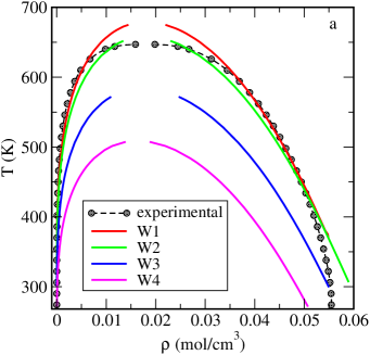
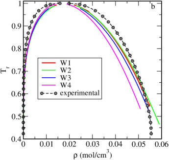
Figure 1: (Colour online) A comparison of the gas-liquid phase diagrams in the density-temperature plane for the W1, W2, W3 and W4 models of water. Panel a is in real units. In panel b, the temperature is rescaled using the bulk critical temperature for each model, $T_{\text{r}}=T/T_{\text{c}}$, cf. table 2. The experimental data (symbols) are from [53, 54].

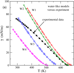
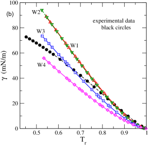
Figure 2: (Colour online) A comparison of the temperature dependence of the surface tension of water from theory for the models W1, W2, W3 and W4 (lines) with experimental data (symbols) [54]. Panel a is in real units, while in panel b the temperature is rescaled by the bulk critical temperature, cf. figure 1.

Figure 1b indicates that the simple mean field approximation used within the SAFT approach is capable of predicting the phase behavior of bulk with reasonable accuracy, if the temperature is appropriately rescaled (note that the temperature rescaling is equivalent with rescaling of the energy parameter $\varepsilon$). Similarly to figure 1a, the results in figure 1b indicate a slight superiority of the models W1 and W2, i.e., the models with low-dispersion and high hydrogen bonding compared to the models with high-dispersion and low hydrogen bonding effects. One important drawback of the description of association effects can be seen in figure 1. Namely, the behavior of the liquid branch at low temperatures is not well captured within the simplified theoretical description here, as well as in the original modelling [22]. This precludes the description of density anomaly of water close to the experimental triple point as well as of the anomaly of isothermal compressibility. These features are out of reach within the present approach, in contrast to water models used in computer simulations [52].

For each potential model, the obtained mean field values for the coexisting dew and bubble densities, $\rho_{\text{bg}}$ and $\rho_{\text{bl}}$, are next used for evaluating the density profiles across the gas-liquid interface at several temperatures and then — the values for the surface tension, $\gamma$ (see figure 2).

In figure 2a, real units are used. However, the quantities from DFT are expressed in reduced, dimensionless units. Therefore, a comment is necessary regarding the conversion of theoretically determined quantities into real units. According to equation (3.17), the surface tension is defined as the surface excess grand thermodynamic potential per unit surface area and the computed values of the surface tension are dimensionless, $\gamma^{*}=\gamma\sigma^{2}/\varepsilon$. To obtain the values of $\gamma$ in mili Newtons per meter, for each model we use the appropriate molecular parameters from table 1. On the other hand, due to the difference of the critical temperatures predicted for the different models in question (see table 2), the surface tension curves in figure 2a end up at different temperatures. Thus, similarly to figure 1b, in figure 2b, we use the rescaled temperature units $T_{\text{r}}=T^{*}/T^{*}_{\text{c}}$. However, for the values of the surface tension we keep the real units. This presentation differs from our previous work [18]. The data displayed in figure 2b indicate that for the models W1 and W2, the theoretical values overestimate the surface tension in comparison with experimental data (especially at lower temperatures $T_{\text{r}}$) while the theoretical data for W3 and W4 models underestimate the surface tension.

The agreement of theoretically predicted values of surface tension with experimental data [54] is not as good as from calculations of Clark et al. [22]. However, the calculations of the surface tension of Clark et al.[22] within the second-order perturbation expansion for the attractive forces follow from a version of the SAFT-DFT by Gloor et al. [55] tested solely for vapor-liquid interfaces. Our data in figure 2 are obtained within the mean field approximation. Moreover, our calculations lead to bigger discrepancies between the values of $\gamma$ for different water-water interaction models in comparison with [22]. Apparently, there remains room for optimization of the parameters of different contributions to the inter-molecular interaction potential within mean field and higher-order approaches to improve the description of the particular property of interest. Cancellation of errors from applied approximations for a given property does not ensure the applicability of the theory in a wider context. Therefore, we proceed now to a more demanding test for the theory by considering water-solid interface.

4.2 Water in contact with solid surfaces. Contact angles

In this subsection of our work we focus on the problem of the description of wetting of solid surfaces for different models of water-water interactions in terms of contact angles. We begin our discussion with the presentation of the temperature dependence of the contact angle, calculated from equation (3.18).

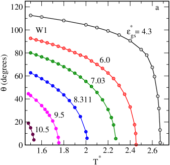
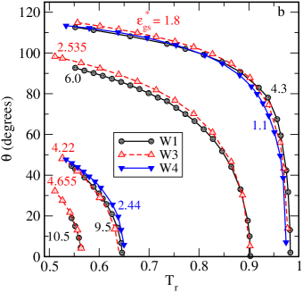
Figure 3: (Colour online) Panel a. Temperature dependence of contact angle for W1 water-like model in contact with various attractive substrates. Panel b. A comparison of the contact angle dependence for different models W1, W3 and W4, on rescaled temperature, $T_{\text{r}}=T^{*}/T_{\text{c}}^{*}$. The values of the fluid-solid attraction, $\varepsilon_{gs}^{*}$ (given in the figure) are chosen to yield similar values of the wetting temperature for different models.

The parameter $\varepsilon_{gs}^{*}$ (cf. equation (4.1)) of the fluid-solid interaction is one of the principal factors determining the adsorption of water and wettability of a given solid surface. In figure 3a we show the values of the contact angle, $\theta$, obtained from equation (3.18) for different values of $\varepsilon_{gs}^{*}$. Panel a is for the model W1. The temperature at which the contact angle drops to zero is the wetting temperature, $T_{w}$. At temperatures higher than $T_{w}$, a given surface is completely wet by liquid water, but at temperatures lower than $T_{w}$ the wetting is only partial. We realize that for $\varepsilon_{gs}^{*}=4.3$, the wetting temperature is very close to the critical temperature of the W1 model (cf. table 2). Therefore, at a slightly lower value of $\varepsilon_{gs}^{*}$, $\varepsilon_{gs}^{*}\approx 4.2$, the surface remains partially wet at all temperatures up to the bulk critical temperature (a precise evaluation of this $\varepsilon_{gs}^{*}$ value is numerically tedious). For high values of $\varepsilon_{gs}^{*}$, the wetting of the surface extends over a wide range of temperatures and, finally, for $\varepsilon_{gs}^{*}\gtrapprox 12$ it is delimited from below by the bulk triple point temperature $T_{\text{t}}$ (the rescaled value is $T_{\text{rt}}=T_{\text{t}}/T_{\text{c}}\approx 0.42$), i.e., wetting occurs at all temperatures for which a gas can coexist with a liquid.

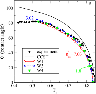
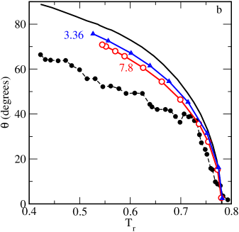
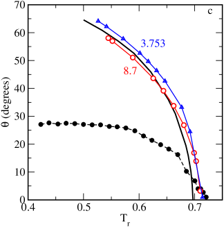
Figure 4: (Colour online) The temperature dependence of the contact angle for W1 and W3 and W4 models for graphite (a), sapphire (b) and quartz (c) surfaces. The $\varepsilon_{gs}^{*}$ values in theoretical calculations are chosen to yield the ratio of the wetting temperature and the bulk critical temperature the same as in experimental measurements [56]. The experimental data are given by black circles. The solid black line in each panel is reproduced from CCST approximation (equation (1) of [56, 57]).

Panel b of figure 3 compares the temperature dependences of $\theta$ for three models W1, W3 and W4. The temperature for each model is rescaled as in the above ($T_{\text{r}}=T^{*}/T_{\text{c}}^{*}$). Since the values of $\varepsilon$ for each model are different, to obtain almost coinciding curves for $\theta(T_{\text{r}})$, different values of $\varepsilon_{gs}^{*}$ should be used. They are listed in the figure. In conclusion, we observe that a very similar temperature dependence of the contact angle is predicted by water-like models with a differing relative weight of inter-particle attraction and association effects. However, the interaction potential strength between the water molecule and solid surface should be chosen appropriately for each model, because the bulk behavior is different in each case.

Usually, a comparison of theoretical predictions with experimental data is not straightforward. In particular, by considering a set of curves in figure 3b, we need to choose the $\varepsilon_{gs}^{*}$ value that corresponds to the experimental graphite. Laboratory measurements of the temperature dependence of the contact angle of water on a highly ordered pyrolytic graphite surface are reported in [56]. The results indicate that the wetting temperature is at $271\pm 12^{\circ}$C. This estimate permits us to put the experimental data on the reduced temperature axis together with theoretical predictions. In our recent study [18], we found that for W1 model and for $\varepsilon_{gs}^{*}=7.03$, the DFT leads to almost the same ratio of the wetting temperature with respect to $T^{*}_{\text{c}}$ as in experiment. For models W3 and W4, the values for $\varepsilon_{gs}^{*}$ are different and equal $\varepsilon_{gs}^{*}=3.02$ and $\varepsilon_{gs}^{*}=1.8$, respectively. Thus, in all cases we found “theoretical” graphite that corresponds to its experimental counterpart for water-like models. The dependences of the contact angle on rescaled temperature for models in question, in comparison with experimental data, are shown in figure 4a. Besides, for the sake of comparison, we also displayed a theoretical curve resulting from the approximation proposed by Cheng, Cole, Saam, and Treiner (CCST) [57] in the same figure 4a. This approximation was derived from the Young equation by making drastic assumptions concerning the gas-solid and liquid-solid interfacial tensions, the expression for the contact angle is given by equation (1) of [56]. From the inspection of all the curves, it follows that our theoretical approach provides an excellent description of the behavior of the contact angle in a rather wide temperature interval. Independent of the water-water interaction model, the results are quite satisfactory. On the other hand, the CCST approximation is not appropriate in this aspect. It overestimates the contact angle values in the entire temperature interval under study.

Similar calculations were carried out for water on sapphire, figure 4b and on quartz, figure 4c. According to the experiment, sapphire surface is slightly more hydrophilic compared to graphite. For this system, the W1 model together with $\varepsilon_{gs}^{*}=7.8$ fits the rescaled experimental wetting temperature. On the other hand, the W3 model together with $\varepsilon_{gs}^{*}=3.36$ satisfy a similar criterion. A satisfactory agreement of theoretical results for both water-like models with the experimental trends on temperature is observed from the wetting temperature down to $\approx 0.75T_{\text{r}}$. At lower temperatures, the theory substantially overestimates the values for the contact angle. Even a more disappointing picture emerges for water on quartz. The $\varepsilon_{gs}^{*}$ values that fit the rescaled wetting temperature are 8.7 and 3.753 for W1 and W3 models, respectively. However, the temperature trends are entirely unsatisfactory. Prediction coming from the CCST approximation is of the same poor quality. Apparent explanation of this behavior seems to be the assumption that the fluid-solid interaction, described by the potential of Steele in equation (2.6), is not appropriate for the description of interaction of water molecules with substrates more hydrophilic than graphite. This is not surprising, because the description of quartz-water interface requires taking account of the chemical aspects of adsorption of water apart from the physics of adsorption, see e.g., computer simulation setup of the problem in [58, 59, 60]. Then, certain ingredients of the theoretical procedure require reconsideration and qualitative modification in order to take account of the bonding between water molecules and hydroxyl groups of the surface.

To summarize this subsection, we would like to mention that the knowledge of the wetting temperature values for different substrates permits to classify them vaguely. If the wetting temperature, $T_{w}$, for a given fluid is close to the bulk critical temperature, $T_{\text{c}}$, one may conclude that the surface is quite hydrophobic or say weakly adsorbing, on intuitive terms. By contrast, if the wetting temperature is far below the critical temperature or closer to the triple point temperature, it is reasonable to term the substrate as strongly adsorbing of hydrophilic. However, a more sound classification of the substrates follows from the inspection of the shape of adsorption isotherms. Hence, in the following subsection we turn our attention to the events observed above the wetting temperature for water-like models on various substrates.

4.3 Water in contact with solid surfaces. Adsorption

If the adsorption from gaseous phase on a solid surface takes place at $T<T_{\text{c}}$, then, dependent on $T$, a different behavior of the adsorbed film thickness can be observed when density approaches the bulk saturated vapor density, $\rho_{\text{bg}}$. The film thickness can either diverge or remain finite and small. The divergence of the film thickness means that the liquid-like film spreads on the surface. On the other hand, a constant value of the adsorbed film thickness at $\rho_{\text{bg}}$ means that the liquid “beads up” on the surface, forming drops. The first scenario corresponds to a complete wetting, whereas the second one — to partial wetting. Hence, the study of wettability can be carried out by measuring or computing the adsorption isotherms from gaseous phase.

A comprehensive classification of different scenarios of adsorption behavior in terms of the phase diagrams was elaborated by Pandit et al. [30] for systems with solely dispersive interactions. It was shown that the principal factor determining the shape of adsorption isotherms on chemical potential for different temperatures is the ratio of the absolute values of energy of fluid-substrate attraction and energy of fluid-fluid attraction, $w$. The latter, in fact, establishes the temperature scale in reduced units. For systems under study, the association between molecules is crucial, although in addition to dispersion interactions. Thus, the ratio $w$ is not sufficient to describe all types of the phase behavior.

It is documented that if $w$ is high, or the substrate is termed as strongly adsorbing, an infinite sequence of first-order transitions, called layering transitions, can be observed on the adsorption isotherm. Each of the layering transitions corresponds to the condensation within a given fluid layer. If the layer number tends to infinity (while the chemical potential approaches the chemical potential of bulk liquid-vapor coexistence, $\mu_{s}$), the critical temperatures for a consecutive layering transition tend to the so-called roughening temperature, $T_{\text{R}}$, which is lower than the bulk critical temperature. At temperatures between $T_{\text{R}}$ and $T_{\text{c}}$, the layering transitions become rounded, and the isotherm diverges upon chemical potential approaching the $\mu_{s}$, see, e.g., figure 1 of [30].

For intermediately attractive substrates, or for lower values of $w$, the gas isotherm can exhibit a single discontinuity at $\mu<\mu_{s}$ (or $\rho_{\text{b}}<\rho_{\text{bg}}$) within a certain interval of temperatures. This discontinuity is the manifestation of prewetting transition. In the chemical potential-temperature plane, the prewetting transition is a line that begins at the bulk liquid-vapor coexistence at the wetting temperature, $T_{w}$. Below the wetting temperature, the adsorption remains finite at the bulk liquid-vapor coexistence. The prewetting line ends up at the prewetting critical point $(\mu(T_{\text{cp}}),T_{\text{cp}})$ and the temperature $T_{\text{cp}}$ is called the prewetting critical temperature. At temperatures above $T_{\text{cp}}$, the adsorbed film thickness grows continuously with increasing bulk density. The entire picture is given in figure 3 of  [30]. A few comments, concerning the shape of adsorption isotherms presented above does not, of course, cover all the possibilities that result from different ratios, $w$. We are interested, however, in these two cases because the water-like model in question on graphite should exhibit similar trends according to our intuition.

In figure 5 we present the temperature dependence of the contact angles and the corresponding estimates for the wetting temperature (upper panel) together with the prewetting phase diagrams following from the behavior of adsorption isotherms (lower panel) for different water-like models and for selected values of $\varepsilon_{gs}^{*}$. The temperature axis is in rescaled units, $T_{\text{r}}=T^{*}/T_{\text{c}}^{*}$. Both methods of determination of the wetting temperature in all cases lead to almost identical values. On the other hand, the models with weaker association effects, W3 and W4, predict a bit longer prewetting lines, or in other words they yield a bit higher values for the prewetting critical temperature, in comparison with the W1 model having a stronger association and weaker effect of non-associative attraction. We should stress, however, that the presented surface phase diagrams (lower panel) include solely the prewetting lines. A set of layering transitions is observed only for the W4 model at $\varepsilon_{gs}^{*}=2.44$, but this particular case will be discussed below.

We are not aware of the experimental results concerning the prewetting critical temperature. To our best knowledge, the prewetting transition of water on graphite was studied using the grand canonical ensemble computer simulation, solely by Zhao [61]. In that study the water-water interactions was considered within the SPC/E model. In figure  5 we compare the prewetting line resulting from simulations (squares) with the DFT predictions for W1 model (line). In theory, the parameter $\varepsilon_{gs}^{*}$ of equation (2.6) was chosen equal to $\varepsilon_{gs}^{*}=8.311$ (this value follows from the Lorentz-Berthelot combination rules). In comparison with the theory, the simulated prewetting line is remarkably shorter indicating a different balance of association and non-association interactions in the theory and computer simulations model.

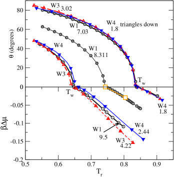
Figure 5: (Colour online) The temperature dependence of the contact angle for W1, W3 and W4 models (upper panel) and the prewetting lines in the temperature-chemical potential plane (lower panel). The values of $\varepsilon_{gs}^{*}$ for each model are given in the figure. The $X$-axis is the rescaled temperature, $T_{\text{r}}=T^{*}/T_{\text{c}}^{*}$, cf. table 2. The variable $\Delta\mu$ is defined as $\Delta\mu=\mu-\mu_{s}$, where $\mu_{s}$ is the chemical potential at the bulk liquid-vapor coexistence.

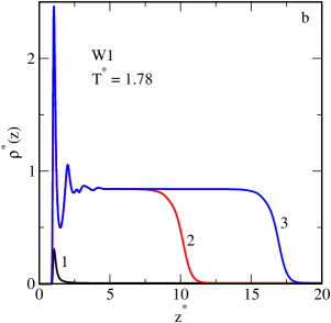
Figure 6: (Colour online) Adsorption isotherm of water-like W1 model just above the wetting temperature at $T^{*}=1.78$ ($T_{\text{r}}=0.655$, $T^{*}_{w}=1.76$) (panel a) and the density profiles of water molecules before and after the prewetting jump and at the final state of calculations. The labels 1 and 2 denote the prewetting jump on the adsorption isotherms. The fluid-solid interaction is: $\varepsilon_{gs}^{*}=9.5$.

The prewetting transition is manifested as a jump on the adsorption isotherm. However, the shape of the adsorption isotherms for different water models can be different. This issue is illustrated in figures 6 and 7. The first of the above figures is for the model W1, while the second is for the model W4. The calculations in each case were carried out at a temperature a bit higher than the wetting temperature, cf. figure 5 ($T_{\text{r}}\approx 0.65$).

For W1 model at $\varepsilon_{gs}^{*}=9.5$ (figure 6), the adsorption isotherm after the prewetting phase transition is smooth and $\Gamma_{\text{ex}}^{*}$ diverges as the chemical potential approaches the bulk liquid-vapor coexistence (panel a). The density profiles of water species at three characteristic values of the chemical potential, marked as 1, 2 and 3 in panel a, are shown in figure 6b. The first value of the chemical potential is just before and the second is just after the prewetting jump on the adsorption isotherm, the third value corresponds to the highest bulk density used in the adsorption isotherm calculations. Before the transition only a small local density peak at the solid surface vicinity appears (figure 6b). After the transition, the adsorbed layer extends up to the distances $z^{*}\approx 10$ ($\Gamma_{\text{ex}}^{*}\approx 8$). A further increase of the chemical potential leads to the growth of the adsorbed film thickness, although the liquid film density remains almost constant. The thickness of the film tends to infinity as $\Delta\mu\to 0$.

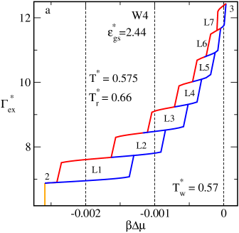
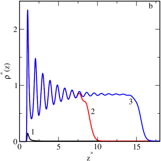
Figure 7: (Colour online) Adsorption isotherm of water-like W4 model just above the wetting temperature at $T^{*}=0.575$ ($T^{*}_{w}=0.57$) (panel a) and the density profiles of water molecules before and after the prewetting jump and at the final state of calculations. The labels 1 and 2 denote the prewetting jump on the adsorption isotherms. The fluid-solid interaction is $\varepsilon_{gs}^{*}=2.44$.

For W4 model at $\varepsilon_{gs}^{*}=2.44$, however, the isotherm consists of a series of discontinuous steps. Except for the first jump, the following, consecutive jumps are associated with the condensation within single consecutive layers. The first jump, however, describes the formation of a thick film on the surface. The excess adsorption increases from $\Gamma_{\text{ex}}^{*}=0.04$ (point 1, similar as in figure 6a - not shown here) before the prewetting transition to $\Gamma_{\text{ex}}^{*}\approx 6.9$ (point 2) after it. The following jumps can be identified as the first-order layering transitions. For each transition that is marked as L1, L2,…, L7, we plotted the spinodals (the equilibrium transitions appear between two spinodal parts). The spinodals correspond to metastable adsorption and desorption branches. If $\Delta\mu$ tends to zero, the calculations become very tedious, since the transitions are located very close to the bulk liquid-vapor coexistence. A set of seven layering transitions is observed at $T^{*}=0.575$. The adsorption branch of the last investigated transition becomes a bit metastable with respect to the bulk liquid-vapor transition.

The first, prewetting jump of the adsorption isotherm for W4 model leads to the formation of the ordered film in the $OZ$-direction. Such a situation was not observed for W1 model, i.e., for the model that is characterized by much stronger association effects than the W4 model. Thus, the layering transitions result from non-association interactions. Actually, the thick ordered film forms a new “adsorbing surface” that attracts water molecules from the gaseous phase. The adsorption on this “new” surface occurs as a series of layerings. However, the ordering in the $OZ$ direction within the consecutive layers becomes less and less pronounced (the oscillations of the local density profile diminish upon increasing the distance from the surface).

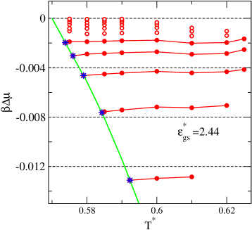
Figure 8: (Colour online) The surface phase diagram in the chemical potential-temperature plane for the model W4. The wetting temperature is $T_{w}^{*}\approx 0.57$. Only a part of the prewetting line (green line) is plotted here. The layerings are marked in red and the five initial triple points are marked as blue asterisks. The fluid-solid interaction is $\varepsilon_{gs}^{*}=2.44$.

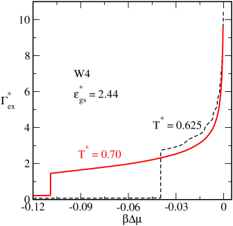
Figure 9: (Colour online) The adsorption isotherms for the W4 model at $T^{*}=0.625$ (dashed line) and at $T^{*}=0.7$ (solid line)

Figure 8 displays a part of the surface phase diagram for the system W4. Each layering transition line meets the prewetting line at the triple point (blue asterisk) and ends up at its own critical point. Complete layering diagrams are evaluated only for five transitions most distant from the bulk coexistence. They are marked with solid circles. With an increase of the layer number, the lines for layering transitions are getting closer to the bulk liquid-vapor coexistence and between themselves. Thus, it becomes very difficult to establish whether all the layerings branches survive with decreasing temperature till the prewetting line or some of them meet at a certain triple point, prior to reaching the prewetting line, in close similarity to the study of Lennard-Jones associating fluid in contact with solid surfaces [28]. The layering transitions closest to the bulk coexistence apparently end up at temperatures above the wetting temperature as in [28].

Definitely, the layerings L3, L4 and L5 are characterized by the higher reduced critical point temperatures $T_{\text{{c}}Li}^{*}\approx 0.625$ ($i=3,4,5$) in comparison with L1 and L2, as well as in comparison with layering transitions closest to the bulk coexistence temperature. At temperatures higher than 0.625, no layerings are present in the system and only the prewetting transition survives, cf. figure 9. Indeed, at $T^{*}=0.625$, the isotherm is smooth, with just three steps layering, which are better seen in figure 8. The second isotherm in figure 9 at $T^{*}=0.7$ exhibits solely the prewetting step. After the prewetting transition, the isotherm is entirely smooth. During the prewetting, the adsorption increases from $\Gamma_{\text{ex}}^{*}\approx 0.23$ to $\Gamma_{\text{ex}}^{*}\approx 1.48$. Thus, this step is much smaller than that observed at $T^{*}=0.575$ (figure 7a). This suggests that the temperature 0.7 is close to the surface critical temperature. Actually the calculations performed at $T^{*}=0.75$ (not shown) lead to a typical isotherm showing a continuous increase and the divergence at the bulk gas-liquid coexistence. We recall (cf. figure 7) that the wetting temperature for the system under study is $T_{w}^{*}=0.57$ and the critical prewetting temperature is close to $T^{*}_{\text{cp}}\approx 0.74$ (see lower panel of figure 5).

The surface phase diagrams evaluated for W1 (figure 5, lower part; as well as figure 3a of [18]) and W4 are qualitatively different. They belong to different classes of the surface phase diagrams, according to the classification of Pandit et al. [30]. However, both these diagrams are evaluated for the values of $\varepsilon_{gs}^{*}$ yielding a similar value of the wetting temperature and a similar dependence of the contact angle, $\theta$, on temperature (in case the temperature is expressed in rescaled units), cf. figure 5. The values of $\varepsilon_{gs}^{*}$ were 9.5 and 2.44 for the models W1 and W4, respectively.

In the case of the W1 model, the entire surface phase diagram consists solely of the prewetting line. For the model W4, however, not only the prewetting transition but also a sequence of layering transitions appears on the diagram. As we have already stressed. these models differ by the balance of the associative and non-associative terms into the free energy functional. Low-dispersion, high hydrogen bonding model, W1, leads to solely prewetting type transition. By contrast, weak chemical association and high dispersion energy between the adsorbed particles in the W4 model enhances the possibility of the development of a thick adsorbed film according to “layer-by-layer” scenario. Otherwise, the reduction of a relative importance of the hydrogen bonds formation causes condensation within consecutive layers, especially at lower temperatures. However, we should emphasize that in spite of certain similarities, the phase diagram presented in figure 8, does not belong to any class of the surface phase diagrams discussed by Pandit et al. [30]. Thus, the overall picture of surface phase transitions in the systems with associative interaction may be much richer than in the systems with solely dispersive forces.

5 Summary and conclusions

In this study we revised the application of a version of the classical density functional approach to investigate interfacial behavior of water at surfaces interacting with the (10-4-3) Lennard-Jones type potential of Steele. Water is modelled by using SAFT methodology with square well attraction between molecules and associative site-site interaction. The four-site model with both dispersion and association potential energies described by square-well potentials with parameters from  [22] have been used. However, in contrast to the original work of Clark et al. [22] and  [55], the contribution to the nonuniform free energy functional resulting from the attractive dispersion (non-associative) forces is approximated by the mean-field term.

The models studied by us can be considered as models ranging from predominant effects of associative interactions compared to non-associative effects models (W1 and W2) to the models (W3 and W4) that are characterized by weaker association and stronger non-associative effects. In the case of bulk fluids, all these models lead to a reasonable description of the bulk phase behavior of water. However, our calculations have indicated that their application to the water-solid interfaces can lead to quite different surface phase diagrams. In particular, the W4 model predicts a sequence of layering transitions, while the model W1 predicts the appearance of the prewetting line only.

A comparison of the wetting behavior with experimental (or simulation [61]) data requires the knowledge of the parameter of the water-surface potential, $\varepsilon_{gs}^{*}$. The method for this choice used by us is based on predicting the wetting temperature and the temperature dependence of the contact angle. Of course, such a method does not ensure that other quantities such as isotherms and heat of adsorption will also be accurately reproduced. The choice of a proper analytical expression for the fluid-solid potential energy is a key problem in predicting the thermodynamic properties of fluid-solid systems. This problem is particularly well seen in the case of the temperature dependence of the contact angle of water on quartz, and to some extend for water on sapphire. Despite the capability to correctly reproduce the wetting temperature, at lower temperatures the values of the contact angle computed from theory significantly differ from experimental results. This may indicate the incorrectness of the potential given by equation (2.6) for these systems. One of possible reasons is that the presence of hydroxyl groups on these surfaces may cause the formation of hydrogen bonds with water. The possibility of formation of such bonds should be taken into account upon further development of the present theory.

In order to compare the results of the present theory with experimental data, we used the rescaling of temperature by the bulk critical temperature. Therefore, the next improvement of the theory would relay the construction of an approach that goes beyond the mean-field approximation. Of course, the mean-field approximation is computationally convenient, in contrast to any approach (e.g., [55, 62]) that takes into account the correlations between the particles in the attractive, non-associative free energy functional. However, all more sophisticated approaches would result in much more computationally demanding procedure. Finally, it could be profitable to use a more sophisticated version of Wertheim’s theory of association, e.g., the second-order theory, like in [63] for water-water hydrogen bonding and/or to take into account water-surface associative forces (particularly for the case of solids with hydroxyl groups on their surfaces). Allowing for surface association, one should also consider a possible competition between water-water and water-surface association, i.e., in order to modify the formulation of the mass action law.

Ukrainian 0

Перегляд поведiнки змочування твердих поверхонь за допомогою моделей води у рамках теорiї функцiоналу густини А. Козiна${}^{\textsf{\footnotesize{\mbox{?}}}}$, М. Агiлар${}^{\textsf{\footnotesize{\mbox{?}}}}$, О. Пiзiо${}^{\textsf{\footnotesize{\mbox{?}}}}$, С. Соколовскi${}^{\textsf{\footnotesize{\mbox{?}}}}$

             
${}^{\textsf{\footnotesize 1}}$ Iнститут хiмiї Нацiонального автономного унiверситету Мехiко, Сiркiто Екстерiор, 04510, Мехiко, Мексика ${}^{\textsf{\footnotesize 2}}$ Факультет теоретичної фiмiї, Унiверситет iм. Марiї Склодовської-Кюрi, Люблiн 20-614, вул. Глиняна 33, Польща

References

- [1] Ilnytskyi J., Wilson M. R., Comput. Phys. Commun., 2002, 134, 23–32, doi:10.1016/S0010-4655(00)00187-9.
- [2] Ilnytskyi J., Toshchevikov V., Saphiannikova M., Soft Matter, 2019, 15, 9894–9908, doi:10.1039/C9SM01853K.
- [3] Ilnytskyi J. M., Wilson M. R., J. Mol. Liq., 2001, 92, 21–28, doi:10.1016/S0167-7322(01)00174-X.
- [4] Sokolowski S., Ilnytskyi J., Pizio O., Condens. Matter Phys., 2014, 17, 12601, doi:10.5488/CMP.17.12601.
- [5] Ilnytskyi J., Patsahan T., Pizio O., J. Mol. Liq., 2016, 223, 707–715, doi:10.1016/j.molliq.2016.08.098.
- [6] Ilnytskyi J., Sokolowski S., Pizio O., Phys. Rev. E, 1999, 5, 4161–4168, doi:10.1103/PhysRevE.59.4161.
- [7] Ilnytsky J., Patrykiejew A., Sokolowski S., Pizio O., J. Phys. Chem. B, 1999, 103, 868–871, doi:10.1021/jp983302.
- [8] De Gennes P.-G., Brochard-Wyart F., Quéré D., Capillarity and Wetting Phenomena: Drops, Bubbles, Pearls, Waves, Springer, New York, 2004, doi:10.1007/978-0-387-21656-0.
- [9] Ruckenstein E., Berim G., Wetting: Theory and Experiments, Two-Volume Set, CRC Press, 1st Ed., Boca Raton, 2018, doi:10.1201/9780429487972.
- [10] Starov V. M., Velarde M. G., Wetting and Spreading Dynamics, CRC Press, 2nd Ed., Boca Raton, 2019, doi:10.1201/9780429506246.
- [11] Bonn D., Eggers J., Indekeu J., Meunier J., Rolley E., Rev. Mod. Phys., 2009 81, 739–805, doi:10.1103/RevModPhys.81.739.
- [12] Anantharaju N., Panchagnula M. V., Vedantam S., In: Contact Angle, Wettability and Adhesion, Vol. 6, Mittal K. L. (Ed.), Koninklijke Brill NV, Leiden, 2009, 53–64, doi:10.1201/b12247.
- [13] Dietrich S., Popescu M. N., Rauscher M., J. Phys.: Condens. Matter, 2005, 17, S577–S593, doi:10.1088/0953-8984/8/47/004.
- [14] Yatsyshin P., Kalliadasis S., J. Fluid Mech., 2021, 913, A45, doi:10.1017/jfm.2020.1167.
- [15] Mistura G., Pierno M., Adv. Phys.: X, 2017, 2, 591–607, doi:10.1080/23746149.2017.1336940.
- [16] Li H., Li A., Zhao Z., Li M., Song Y., Small, 2020, 1, 2000028, doi:10.1002/sstr.202000028.
- [17] Wang J., Xiao L., Liao G., Zhang Y., Guo L., Arns C. H., Sun Z., Sci. Rep., 2018, 8, 1–14, doi:10.1038/s41598-018-31803-w.
- [18] Pizio O., Sokolowski S., Mol. Phys, 2022, 120, e2011454, doi:10.1080/00268976.2021.2011454.
- [19] Pizio O., Sokołowski S., In: Encyclopedia of Solid-Liquid Interfaces, Elsevier, 2024, 114–125, doi:10.1016/B978-0-323-85669-0.00067-2.
- [20] Pusztai L., Pizio O., Sokolowski S., J. Chem. Phys., 2008, 129, 184103, doi:10.1063/1.2976578.
- [21] Müller E. A., Gubbins K. E., Ind. Eng. Chem. Res., 2001, 40, 2193, doi:10.1021/ie000773w.
- [22] Clark G. N., Haslam A. J., Galindo A., Jackson G., Mol. Phys., 2006, 104 3561–3581, doi:10.1080/00268970601081475.
- [23] Zhao H., Ding Y., McCabe C., J. Chem. Phys., 2007, 127, 084514, doi:10.1063/1.2756038.
- [24] Patrykiejew A., Sokolowski S., Pizio O., In: Surface and interface science: Solid-gas interfaces II, Vol. 6, Wandelt K. (Ed.), chap. 46, John Wiley & Sons, Ltd, 2016, 883–1253, doi:10.1002/9783527680580.ch46.
- [25] Yu Y.-X., Wu J., J. Chem. Phys., 2002, 116, 7094–7103, doi:10.1063/1.1463435.
- [26] Haghmoradi A., Wang L., Chapman W. G., J. Phys.: Condens. Matter, 2017, 29, 044002, doi:10.1088/1361-648x/29/4/044002.
- [27] Bryk P., Sokolowski S., Pizio O., J. Chem. Phys., 2006, 125, 024909, doi:10.1063/1.2212944.
- [28] Millan Malo B., Huerta A., Pizio O., Sokolowski S., J. Phys. Chem. B, 2000, 104, 7756–7763, doi:10.1021/jp000731l.
- [29] Dufal S., Lafitte T., Haslam A. J., Galindo A., Clark G. N. I., Vega C., Jackson G., Mol. Phys., 2015, 113, 948–984, doi:10.1080/00268976.2015.1029027.
- [30] Pandit R., Schick M., Wortis M., Phys. Rev. B, 1982, 26, 5112–5140, doi:10.1103/PhysRevB.26.5112.
- [31] Hughes A. P., Archer A. J., Thiele U., Amer. J. Phys., 2014, 82, 1119–1129, doi:10.1119/1.4890823.
- [32] Jackson G., Chapman W. G., Gubbins K. E., Mol. Phys., 1988, 65, 1–31, doi:10.1080/00268978800100821.
- [33] Barker J., Henderson D., J. Chem. Phys., 1967, 47, 4714–4721, doi:10.1063/1.1701689.
- [34] Steele W. A., The Interaction of Gases with Solid Surfaces, Pergamon Press, Oxford, 1974.
- [35] Wertheim M. S., J. Stat. Phys., 1984, 35, 19–34, doi:10.1007/BF01017362.
- [36] Wertheim M. S., J. Stat. Phys., 1984, 35, 35–47, doi:10.1007/BF01017363.
- [37] Chapman W. G., Jackson G., Gubbins K. E., Mol. Phys., 1988, 65, 1057–1079, doi:10.1080/00268978800101601.
- [38] Gil-Villegas A., Galindo A., Whitehead P. J., Mills S. J., Jackson G., Burgess A. N., J. Chem. Phys., 1997, 106, 4168–4186, doi:10.1063/1.473101.
- [39] Trejos V. M., Pizio O., Sokolowski S., Fluid Phase Equilib., 2018, 473, 145–153, doi:10.1016/j.fluid.2018.06.005.
- [40] Pizio O., Sokolowski S., J. Mol. Liq., 2022, 357, 119111, doi:10.1016/j.molliq.2022.119111.
- [41] Pizio O., Sokolowski S., J. Mol. Liq., 2023, 390, 123009, doi:10.1016/j.molliq.2023.123009.
- [42] Yu Y-X., Wu J., J. Chem. Phys., 2002, 117, 10156–10164, doi:10.1063/1.1520530.
- [43] Trejos V. M., Pizio O., Sokolowski S., J. Chem. Phys., 2018, 149, 134701, doi:10.1063/1.5066552.
- [44] Pizio O., Trejos V. M., Sokolowski S., Mol. Phys., 2020, 118, 1615647, doi:10.1080/00268976.2019.1615647.
- [45] Bryk P., Bucior K., Sokolowski S., Żukociński G., J. Phys.: Condens. Matter, 2004, 16, 8861–8873, doi:10.1088/0953-8984/16/49/005.
- [46] Dietrich S., In: Phase Transition and Critical Phenomena, Vol. 12, Domb C., Lebowitz J. L. (Eds.), Academic Press, London, 1988, 2–218.
- [47] Fox H. W., Zisman W. A., J. Colloid Sci., 1950, 5, 514–531, doi:10.1016/0095-8522(50)90044-4.
- [48] Jasper W. J., Anand N., J. Mol. Liq., 2019, 281, 196–203, doi:10.1016/j.molliq.2019.02.039.
- [49] Rapaport D. C., The Art of Molecular Dynamics Simulation, Cambridge University Press, Cambridge, 2004, doi:10.1017/CBO9780511816581.
- [50] Heyes D. M., CMST, 2015, 21, 169–179, doi:10.12921/cmst.2015.21.04.001.
- [51] Pizio O., Sokolowski S., Trejos V. M., Condens. Matter Phys., 2021, 24, 33601, doi:10.5488/CMP.24.33601.
- [52] Pi H., Aragones J. L., Vega C., Noya E. G., Abascal J. L. F., Gonzalez M. A., McBride C., Mol. Phys., 2009, 107, 365–374, doi:10.1080/00268970902784926.
- [53] Fletcher D. A., McMeeking R. F., Parkin D., J. Chem. Inf. Comput. Sci., 1966, 36, 746, doi:10.1021/ci960015+.
- [54] Vargaftik N. B., Volkov B. N., Voljak L. D., J. Phys. Chem. Ref. Data, 1983, 12, 817–820, doi:10.1063/1.555688.
- [55] Gloor G. J., Jackson G., Blas F. J., Martin del Rio E., de Miguel E., J. Chem. Phys., 2004, 121, 12740, doi:10.1063/1.1807833.
- [56] Friedman S. R., Khalil M., Taborek P., Phys. Rev. Lett., 2013, 111, 226101, doi:10.1103/PhysRevLett.111.226101.
- [57] Cheng E., Cole M. W., Saam W. F., Treiner J., Phys. Rev. Lett., 1991, 67, 1007–1011, doi:10.1103/PhysRevLett.67.1007.
- [58] Notman R., Walsh T. R., Langmuir, 2009, 25, 1638–1644, doi:10.1021/la803324x.
- [59] De Leeuw N. H., Higgins F. M., Parker S. C., J. Phys. Chem. B, 1999, 103, 1270–1277. doi:10.1021/jp983239z.
- [60] Gaigeot M.-P., Sprik M., Sulpizi M., J. Phys.: Condens. Matter, 2012, 24, 124106, doi:10.1088/0953-8984/24/12/124106.
- [61] Zhao X., Phys. Rev. B, 2007, 76, 041402(R), doi:10.1103/PhysRevB.76.041402.
- [62] Sokolowski S., Fischer J., J. Chem. Phys., 1992, 96, 5441–5447, doi:10.1063/1.462727.
- [63] Sokolowski S., Kalyuzhnyi Y. V., J. Phys. Chem. B, 2014, 118, 9076–9084, doi:10.1021/jp503826p.
Ukrainian \adddialect\l@ukrainian0 \l@ukrainian