Competition for binding targets results in paradoxical effects for simultaneous activator and repressor action - Extended Version

Abstract

In the context of epigenetic transformations in cancer metastasis, a puzzling effect was recently discovered, in which the elimination (knock-out) of an activating regulatory element leads to increased (rather than decreased) activity of the element being regulated. It has been postulated that this paradoxical behavior can be explained by activating and repressing transcription factors competing for binding to other possible targets. It is very difficult to prove this hypothesis in mammalian cells, due to the large number of potential players and the complexity of endogenous intracellular regulatory networks. Instead, this paper analyzes this issue through an analogous synthetic biology construct which aims to reproduce the paradoxical behavior using standard bacterial gene expression networks. The paper first reviews the motivating cancer biology work, and then describes a proposed synthetic construct. A mathematical model is formulated, and basic properties of uniqueness of steady states and convergence to equilibria are established, as well as an identification of parameter regimes which should lead to observing such paradoxical phenomena (more activator leads to less activity at steady state). A proof is also given to show that this is a steady-state property, and for initial transients the phenomenon will not be observed. This work adds to the general line of work of resource competition in synthetic circuits.

I INTRODUCTION AND BACKGROUND

The field of synthetic biology has as its ultimate goal to program new or modify existing biological systems, for applications ranging from cell therapies and regenerative medicine to biosensing and biofuel production. In general, a significant obstacle to the development of synthetic biological circuits is the influence of compositional context: the fundamental characteristics of a circuit alter in the presence of additional components due to competition for resources, off-target interactions, genetic context, growth rate feedback loops, and retroactivity effects. See e.g. [1, 2, 3, 4, 5, 6] and [7] for an overview, Unless one designs mathematically-validated control circuits to compensate for uncertainty, designers will need to re-adjust each part whenever new elements are integrated into a system.

In general, a significant obstacle to the development of synthetic biological circuits is the influence of compositional context: the fundamental characteristics of a circuit alter in the presence of additional components due to competition for resources and retroactivity effects. Unless one designs mathematically-validated control circuits to compensate for uncertainty, designers need to re-adjust each part whenever new elements are integrated into a system.

In this paper, we study a synthetic design that aims to validate the competition principles in a model from [8] that has been hypothesised to explain a paradoxical effect in cell differentiation experiments. The transformation of genetically identical cells into distinct phenotypes, and the transitions between these phenotypes, are governed by complex processes involving epigenetic markers as well as more classical gene-regulatory networks (GRNs) involving transcription factors and non-coding regulatory RNAs. In living cells, such interactions are complicated by the potential competition of multiple TFs over one target, and also by the sequestration of a TF by multiple targets. However, it is not entirely clear whether such effects are able to drive cellular decision making. In a recent publication [8], we have hypothesised that the competition for genomic targets among epigenetic factors can provide an explanation for puzzling experimental data regarding the epithelial–mesenchymal transition (EMT) in cancer metastasis. Our mathematical analysis predicted that when the activity of a regulator is perturbed, it can lead to the widespread redistribution of epigenetic marks, thereby influencing the levels of competing regulators.

Since it is hard to test this mechanistic hypothesis through epigenetic modifications in mammalian cells, we propose here a synthetic biology analog involving transcription factors in bacterial cells. In this paper, we review the mechanism and make mathematical predictions from a model, as well as a proposed implementation using CRISPR/a technology. Experimental work is ongoing. In the remainder of this section, we review our previous results [8].

I-A Review of previous work

Regulatory factors competing for the same target. Depending on the nature of a regulator, its target can be a promoter, a histone tail, an mRNA, or others. However, mathematically, we can represent the state of a given target using the same simplified three-state model depicted in Figure 1.

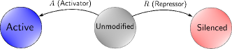
Figure 1: A simplified model of a target that can occupy three different states.

If a target has not been subject to the activity of a regulator, it retains its nominal state which we call “unmodified”. A regulator can change the nominal state into “active” or “silenced” depending on whether it is an activator or repressor, respectively. If the a target is subject to the activity of regulators with opposing effects, then it can switch between the three different states depending on the binding affinities and the abundances of the regulators.

Motivation: Experiments on a cancer cell line. Epigenetic regulation has many examples in which opposing regulators compete for the same targets. A prominent example is the antagonism between the Polycomb complex group (PcG) and the Trithorax (TrX) group [9]. This system has been probed in a recent set of knockout experiments in a breast cancer cell line [10] using CRISPR. The knockout of PRC2 (a PcG repressor) and KMT2D (a TrX activator) initiated two distinct trajectories of epithelial-to-mesenchymal transitions (EMTs). Using the language of dynamical systems, the system settled into two different steady states depending on the particular perturbation.

Motivation: Paradoxical gene activity pattern. In the aforementioned experiments, a paradoxical pattern of gene activation was observed that cannot be easily explained by known local gene regulatory interactions. Consider a gene of interest (e.g, ZEB1 which is a major driver of EMT). As shown in Figure 2,

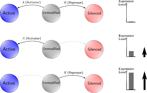
Figure 2: Paradoxical results of the knockout experiments from [10]. Knockout of a repressor is not able to restore the full activity of a target gene (e.g, ZEB1), while knocking out an activator results in maximal activation.

the gene is nominally repressed due to the dominant activity of the repressor (PRC2). However, when the repressor is knocked out, the gene achieves a mediocre amount of activation. In the second knockout experiment, an activating regulator (KMT2D) is knocked out. In that case, the gene achieves maximal activation despite the fact that its main repressor is not knocked-out. The main question is: how would the direct knockout of a repressing regulator be less effective in activating a gene compared to knocking out an activator?. We summarize our answer next.

Our model: off-target competition causes sequestration. In our recent paper [8], we reviewed the relevant literature on PcG/TrX regulators and distilled it into four postulates:

1. Regulators compete for binding to the same targets.

2. There is a large number of targets per regulator, e.g hundreds or thousands.

3. Each regulator has limited levels.

4. When a regulator molecule is active at a given target, it cannot influence the activity of other targets.

Toy model with two factors. Consider a toy model of two regulators competing for a target as shown in Figure 3.

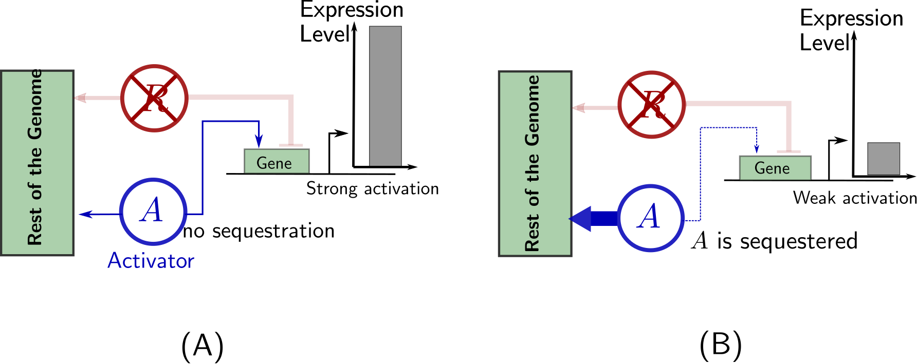
Figure 3: Repressor knockout case. (A) global context has no effect. (B) global context has considerable effect.

In the absence of regulators, the target is assumed to be weakly active. When the regulators are present, assume that the repressor is dominant and it is able to robustly silence the target. Let us consider an experiment in which the repressor in knocked out. In a situation in which there is minimal off-target interference, we expect that the activator utilizes the absence of its competitor to strongly activate its target as shown in Figure 3-a). However, assume now that the activator shares many other targets with the repressor across the genome, and once the repressor knockout, a “void” is created across the genome, and the activator has too many potential targets. Depending on the relative affinities, the activator can get sequestered into other targets across the genome leaving out the target gene without activation as shown in Figure 3-b). The opposite scenario can be similarly illustrated as in Figure 4 where the repressor is still nominally dominant. When the activator is knocked out, the repressor can silence the target when there is minimal off-target interference as shown in Figure 4-a).

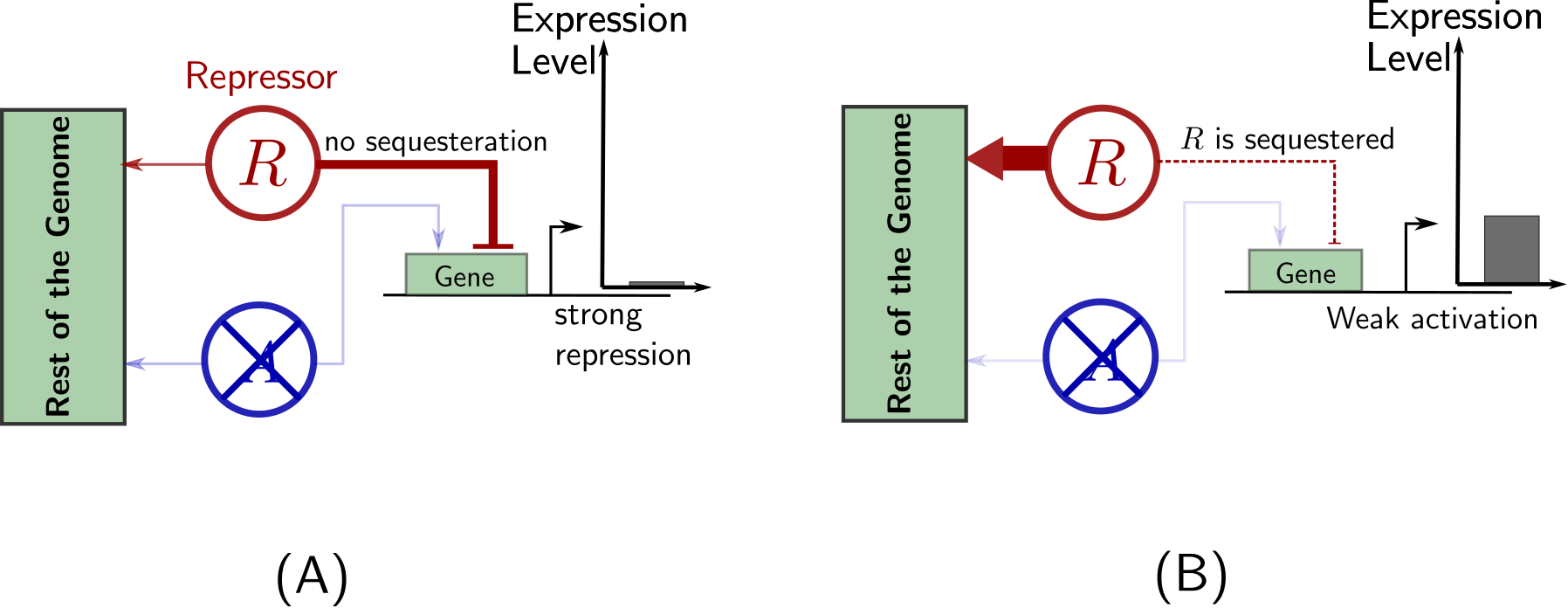
Figure 4: Activator knockout case. (A) global context has no effect. (B) global context has considerable effect.

However, the repressor can get sequestered to other off-targets when there is significant affinity to off-targets as shown in Figure 4-b), and hence an activator can indirectly activate a target gene by its absence.

This simplified model can partially explain the paradoxical results shown in Figure 2. It shows how repressor knockout can fail to activate a target gene, and how can an activator knockout activate the target. However, it does not show how can an activator knockout be more effective at activation than a repressor knockout. This is since the mechanism of activation depends on the sequestration of the repressor, hence it cannot yield an activation that is stronger than a full repressor knockout. We tackle this issue next.

The overall model. In order to recapture the full behavior in Figure 2, we need to add a second activator to the two factor model in Figure 4, as shown in Figure 5-a).

When the activator $A$ is knocked out and the repressor $R$ is sequestered by off-targets, the activator $A^{\prime}$ faces no longer any competition and can activate the target gene fully. A natural question might arise: when the repressor is knocked out in Figure 5-b), why cannot $A^{\prime}$ activate the target? The answer lies in the asymmetry in competition for off-targets. This model requires both $A,A^{\prime}$ to be sequestered when $R$ is knocked-out, but only $R$ being sequestered when $A$ is knocked out. This can be realized when each of them has different affinities for the target gene and the off-targets. Therefore, the overall model is depicted in Figure 5.

More generally, our model can admit all possible expressions levels for the three experimental scenarios. This is achieved by varying two parameters per regulator: a “local” association ratio, and a “global” association ratio, where the first describes the binding affinity of the regulator to a target of interest, while the second describes it binding affinity to off-targets. More details are available in [8].

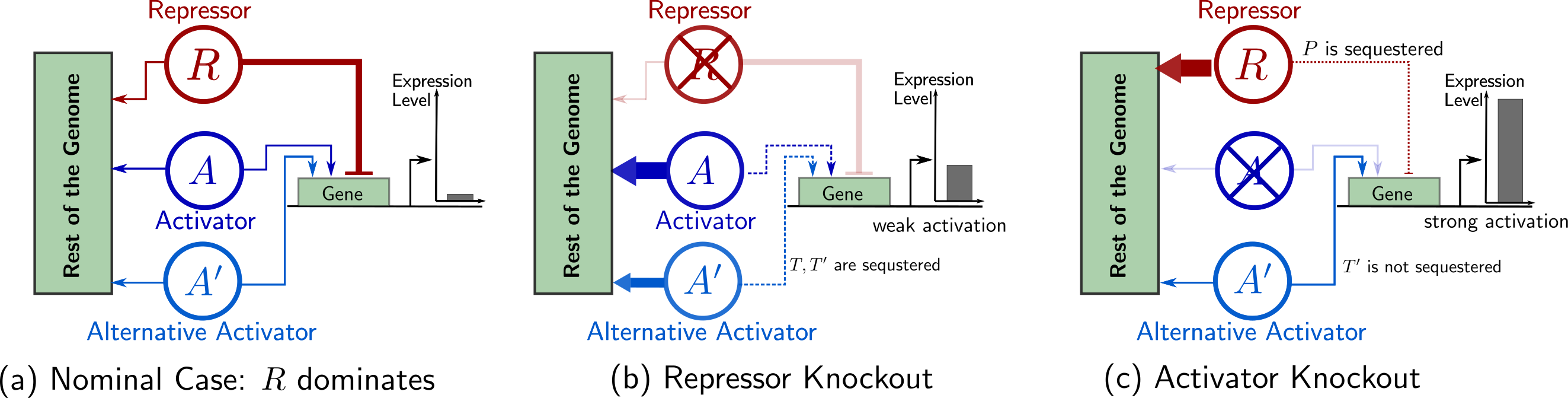
Figure 5: The three-factor model that can explain paradoxical behaviors in gene expression upon knockouts.

As explained in the introduction, it is very difficult to test this mechanistic explanation of the paradoxical effects through epigenetic modifications in mammalian cells. Thus, in this work, we describe and analyze a synthetic biology analog that uses transcription factors in bacterial cells. We start with building the two-factor model, while the three factor model is planned for subsequent work.

II Proposed synthetic construct

The proposed circuit (shown in Figure 6) consists of a pool of shared resources, activators, and repressors, regulating the production of the output protein by the target gene while competing with the rest of the genome, modeled as decoy sites.

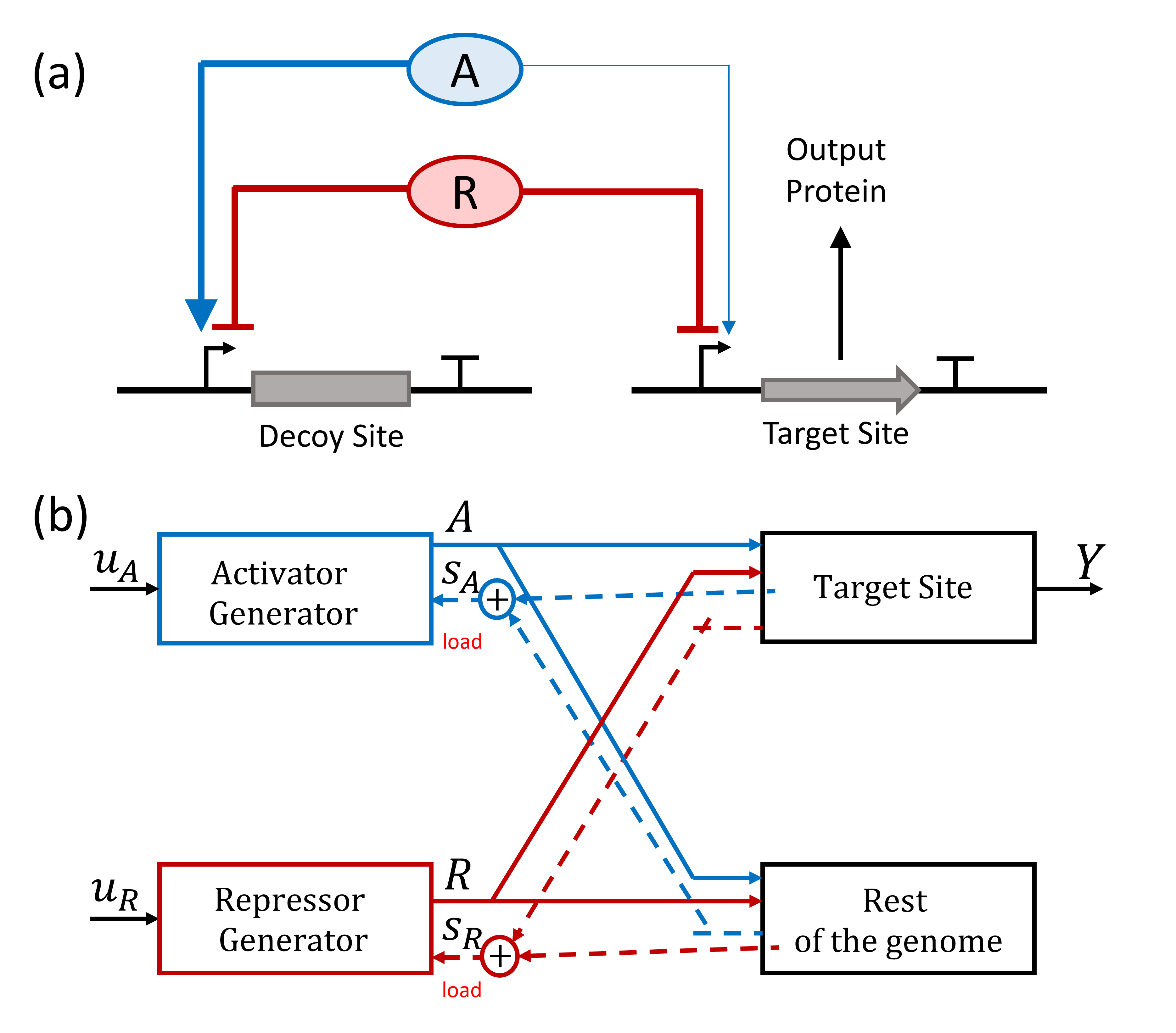
Figure 6: Proposed project: a synthetic competition circuit. (a) Genetic circuit diagram and (b) block diagram representation of the proposed system. Solid lines denote the intended input and outputs and the dashed lines display the unintended loads due to competition in the circuit.

The transcription factors, activator ($A$, produced at a constant rate $u_{A}$) and repressor ($R$, produced at a constant rate $u_{R}$) bind to the target sites to transform into an active form ($T_{A}$) and silenced form ($T_{R}$). The active form of the target undergoes transcription and translation to produce the output protein at a rate $\kappa>\beta$, where $\beta$ is the basal transcription rate in the inactive form of the target. The decoy sites ($D$) sequester the resources by forming $D_{A}$ and $D_{R}$ complexes respectively. The chemical reactions involved are:

$$\emptyset \xrightleftharpoons[\bar{\delta}]{u_{A}}A \emptyset \xrightleftharpoons[\bar{\delta}]{u_{R}}R$$

$$R+T \xrightleftharpoons[t_{r}^{-}]{t_{r}^{+}}T_{R}, A+T \xrightleftharpoons[t_{a}^{-}]{t_{a}^{+}}T_{A}~{}~{}\mbox{(Target)}$$

$$R+D \xrightleftharpoons[d_{r}^{-}]{d_{r}^{+}}D_{R} A+D \xrightleftharpoons[d_{a}^{-}]{d_{a}^{+}}D_{A}~{}\mbox{(Decoy)}$$

$$T_{A} \xrightarrow{\kappa}Y+T_{A} T \xrightarrow{\beta}Y+T$$

$$\{D_{A},D_{R}\} \xrightarrow{\bar{\delta}}D \{T_{A},T_{R}\} \xrightarrow{\bar{\delta}}T$$

$$Y \xrightarrow{\gamma}\emptyset$$ (1)

The corresponding reaction rate equations (RREs) can be obtained using mass action kinetics as [11]:

$$\dot{D_{A}} =d_{a}^{+}DA-d_{a}^{-}D_{A}-\bar{\delta}D_{A}$$ (2)

$$\dot{D_{R}} =d_{r}^{+}DR-d_{r}^{-}D_{R}-\bar{\delta}D_{R}$$ (3)

$$\dot{T_{A}} =t_{a}^{+}TA-t_{a}^{-}T_{A}-\bar{\delta}T_{A}$$ (4)

$$\dot{T_{R}} =t_{r}^{+}TR-t_{r}^{-}T_{R}-\bar{\delta}T_{R}$$ (5)

$$\dot{Y} =\beta T+\kappa T_{A}-\gamma Y,$$ (6)

where $\gamma$ and $\bar{\delta}$ are the corresponding decay rates constant for the protein and complexes. In this system, the total concentrations of the activator, repressor, target and decoy sites are conserved:

$$A_{{\textsc{t}}} =A+T_{A}+D_{A}, R_{{\textsc{t}}}=R+T_{R}+D_{R}$$ (7)

$$T_{{\textsc{t}}} =T+T_{A}+T_{R}, D_{{\textsc{t}}}=D+D_{A}+D_{R}.$$ (8)

III Paradoxical effects at steady state and transients

For the proposed synthetic circuit governed by equations (2)-(8), the paradoxical effect is captured in two scenarios. First, by varying the levels of activator in the circuit (by changing $u_{A}$) and second by varying the levels of decoy sites in the system. The knockout of the activator binding to the target is achieved by maintaining a high dissociation constant $k_{ta}=\tfrac{t_{a}^{-}}{t_{a}^{+}}$.

III-A Increasing activator causing unintended repression

Theorem 1

The proposed synthetic circuit exhibits the paradoxical effect given by:

$$\frac{\mathrm{d}\bar{Y}}{\mathrm{d}u_{A}}<0,\qquad\text{as}\qquad k_{ta}\rightarrow\infty$$

where $\bar{Y}$ is the steady-state levels of the protein when other inputs ($u_{R}$) and parameters ($D_{{\textsc{t}}}$, $T_{{\textsc{t}}}$, reaction rate constants) are kept constant.

Proof.  Using equation (6), the steady-state levels of the output protein is:

$$\overline{Y}=\frac{\beta\overline{T}+\kappa\overline{T_{A}}}{\gamma}$$

where $\overline{x}$ is the steady-state concentration of $x$. At steady state, we have:

$$\overline{D}_{A} =\frac{\overline{D}\overline{A}}{K_{da}},\qquad\overline{T}_{A}=\frac{\overline{T}\overline{A}}{K_{ta}},$$ (9)

$$\overline{D}_{R} =\frac{\overline{D}\overline{R}}{K_{dr}},\qquad\overline{T}_{R}=\frac{\overline{T}\overline{R}}{K_{tr}},$$ (10)

where $K_{xy}=\tfrac{x_{y}^{-}+\bar{\delta}}{x_{y}^{+}}$. Note that as $k_{ta}\rightarrow\infty K_{ta}\rightarrow\infty$ for a finite $\bar{\delta}$. Substituting in equations (7)-(8), we get:

$$\overline{A_{{\textsc{t}}}} =\overline{A}+\frac{\overline{T}\overline{A}}{K_{ta}}+\frac{\overline{D}\overline{A}}{K_{da}}, \overline{R_{{\textsc{t}}}}= \overline{R}+\frac{\overline{T}\overline{R}}{K_{tr}}+\frac{\overline{D}\overline{R}}{K_{dr}},$$ (11)

$$\overline{T_{{\textsc{t}}}} =\overline{T}+\frac{\overline{T}\overline{A}}{K_{ta}}+\frac{\overline{T}\overline{R}}{K_{tr}}, \overline{D_{{\textsc{t}}}}= \overline{D}+\frac{\overline{D}\overline{A}}{K_{da}}+\frac{\overline{D}\overline{R}}{K_{dr}},$$ (12)

$$\therefore\overline{T} =\frac{\overline{T_{{\textsc{t}}}}}{1+\frac{\overline{A}}{K_{ta}}+\frac{\overline{R}}{K_{tr}}}, \overline{D}= \frac{\overline{D_{{\textsc{t}}}}}{1+\frac{\overline{A}}{K_{da}}+\frac{\overline{R}}{K_{dr}}}.$$ (13)

The paradoxical effect is shown by calculating:

$$\frac{\mathrm{d}\overline{Y}}{\mathrm{d}u_{A}}=\frac{\beta}{\gamma}\frac{\mathrm{d}\overline{T}}{\mathrm{d}u_{A}}+\frac{\kappa}{\gamma}\frac{\mathrm{d}\overline{T}_{A}}{\mathrm{d}u_{A}}=\frac{\beta}{\gamma\bar{\delta}}\frac{\mathrm{d}\overline{T}}{\mathrm{d}A_{{\textsc{t}}}}+\frac{\kappa}{\gamma\bar{\delta}}\frac{\mathrm{d}\overline{T}_{A}}{\mathrm{d}A_{{\textsc{t}}}}.$$

Applying product rule after substituting equation (9) in (13):

$$\frac{\mathrm{d}\overline{Y}}{\mathrm{d}u_{A}}=\frac{1}{\gamma\bar{\delta}}\left[\frac{\kappa\overline{A}+\beta K_{ta}}{K_{ta}}\frac{\mathrm{d\overline{T}}}{\mathrm{d}A_{{\textsc{t}}}}+\frac{\kappa\overline{T}}{K_{ta}}\frac{\mathrm{d\overline{A}}}{\mathrm{d}A_{{\textsc{t}}}}\right]$$

Differentiating equation (13) with $A_{{\textsc{t}}}$ and substituting:

$$\frac{\mathrm{d}\overline{Y}}{\mathrm{d}u_{A}}=\frac{1}{\gamma\bar{\delta}} \left(\frac{\kappa\overline{T}}{K_{ta}}-\frac{\kappa\overline{A}+\beta K_{ta}}{K_{ta}}\frac{\overline{T}}{K_{ta}+\overline{A}+\frac{\overline{R}K_{ta}}{K_{tr}}}\right)\frac{\mathrm{d\overline{A}}}{\mathrm{d}A_{{\textsc{t}}}}$$

$$-\frac{\kappa\overline{A}+\beta K_{ta}}{K_{ta}}\frac{\overline{T}}{K_{tr}+\overline{R}+\frac{\overline{A}K_{tr}}{\gamma\bar{\delta}K_{ta}}}\frac{\mathrm{d\overline{R}}}{\mathrm{d}A_{{\textsc{t}}}}$$ (14)

Calculating each derivative individually using equation (11) and substituting in equation (14) and then applying the limit of $K_{ta}\rightarrow\infty$, we get:

$$\frac{\mathrm{d}\overline{Y}}{\mathrm{d}u_{A}}=g_{1}(\overline{A},\overline{R})g_{2}(\overline{A},\overline{R})<0$$ (15)

with

$$g_{2}(\overline{A},\overline{R}):=\left[\frac{g_{3}(\overline{A},\overline{R})}{K_{ta}}-\frac{\beta\overline{R}D_{{\textsc{t}}}}{K_{tr}K_{da}K_{dr}[1+\frac{\overline{R}}{K_{dr}}+\frac{\overline{A}}{K_{da}}]^{2}}\right]$$

where $g_{3}(\overline{A},\overline{R})>0$ and $g_{1}(\overline{A},\overline{R})>0$ for all $\overline{A}>0$ and $\overline{R}>0$. Note that the existence of the conservation law ensures the concentration levels of $\overline{A},\overline{R},\overline{T}$ and $\overline{D}$ are strictly positive under the limit of $K_{ta}\rightarrow\infty$, for any positive value of the total concentration levels ($\overline{A}_{{\textsc{t}}},\overline{R}_{{\textsc{t}}},\overline{T}_{{\textsc{t}}}$ and $\overline{D}_{{\textsc{t}}}$). Details of these computations, including complete expressions for $g_{1}$ and$g_{3}$, are provided in the appendix.  

Figure 7: Paradoxical effect in steady-state levels of the output protein portrayed for varying the levels of (a) activator input levels ($u_{A}$ for $D_{\textsc{t}}=20$) and (b) total decoy sites ($D_{{\textsc{t}}}$ for $u_{A}=10$) in the system. Two parameter bifurcation plots between $u_{A}$ and $D_{\textsc{t}}$ showing the existence of the paradoxical effects for (c) $K_{ta}\rightarrow\infty$ and its absence for (d) $K_{ta}=0.1$. The parameter values used for the simulation are: $K_{tr}=0.1,K_{dr}=0.1.K_{da}=0.1,T_{\textsc{t}}=1,R_{\textsc{t}}=10,\kappa=1000,\beta=100,\text{ and }\gamma=1$.

Figure 7 (a) shows the exhibition of paradoxical effect with increasing the input inducer levels of the activator. As $u_{A}$ is increased, the total amount of activators in the system increases. For low values of $K_{ta}$ ($K_{ta}=0.1$ and 1), the output protein level increases as expected with an increase in the levels of activator. Increasing $K_{ta}$ (to 10 and 100) and thereby gradually knocking out the direct influence of the activator on the target engenders the paradoxical effect, where increasing $u_{A}$ leads to an initial decrease in the output levels of $\overline{Y}$ followed by an increase. For the extreme case of complete knockout of the activator with $K_{ta}\rightarrow\infty$, we observe a monotonic decrease in the concentration of the protein. In the two-parameter bifurcation plots in Figure 7 (c), we see that for high $K_{ta}$ value, the paradoxical affect is observed only after a threshold value of $D_{\textsc{t}}$. For low values of $D_{\textsc{t}}$ (say $10^{0}$), increasing the activator levels have no significant effects on the output protein levels. On the other hand for high $D_{\textsc{t}}$ (say $10^{2}$), increasing the activator levels shows a decrease in the output protein levels hence the paradoxical effect. In the case of low $K_{ta}$ value in Figure 7 (d), we see that increasing $u_{A}$, increases the protein levels irrespective of the value of $D_{{\textsc{t}}}$.

Corollary 1.1

The presence of basal expression is necessary for the exhibition of the paradoxical effect.

Proof.  The presence of basal expression is captured by $\beta$, transcription rate in the inactive/neutral form of the target. Substituting $\beta=0$ in equation (15):

$$\frac{\mathrm{d}\overline{Y}}{\mathrm{d}u_{A}}=g_{1}(A,R)\left[\frac{g_{3}(A,R)}{K_{ta}}\right]>0$$

where $g_{3}(A,R)>0$ and $g_{1}(A,R)>0$ for all $A>0$ and $R>0$. Therefore, increasing the amount of activator causes an increase in the output levels irrespective of the value of $K_{ta}$.  

III-B Dynamics flip during initial transient

To examine the onset of the paradoxical effect, we determine the small-time relationship between the output $Y$ and the input $u_{A}$. We can represent the system under consideration as $\dot{x}=f(x,p)$ where $p$ is the set of parameters (i.e., rate constants) that the system depends on and $x=\{T_{R},T_{A},D_{R},D_{A},Y,A_{{\textsc{t}}},R_{{\textsc{t}}}\}$. We define $Y(x(t))$ as the projection onto the $Y$ species. We indicate the Lie derivative by $L_{{\scriptscriptstyle f(x,p)}}Y(x(t))=(\nabla Y)f(x,p)=\frac{dY}{dt}$.

Theorem 2

For the proposed synthetic circuit governed by equations (2)-(8) with $Y(t,u_{A})$ as a function of $t$ and $u_{A}$, we have:

$$\partial_{u_{A}}Y(t,u_{A})>0$$

for small enough $t$,

$$\partial_{u_{A}}Y(0,u_{a})=\partial_{u_{a}}\dot{Y}(0,u_{a})=\partial_{u_{a}}\ddot{Y}(0,u_{a})=0$$

and

$$\partial_{u_{a}}\dddot{Y}(0,u_{a})=(\kappa-\beta)t_{a}^{+}(T_{{\textsc{t}}}-T_{R}-T_{A}).$$

Proof.  From equation (6), we have that

$$L_{{\scriptscriptstyle f(x,p)}}Y(x(t))=\beta(T_{{\textsc{t}}}-T_{R}-T_{A})+\kappa T_{A}-\gamma Y.$$ (16)

Therefore:

$$L_{{\scriptscriptstyle f(x,p)}}(L_{{\scriptscriptstyle f(x,p)}}Y(x(t)))=\\ \beta(-(t_{r}^{+}(T_{{\textsc{t}}}-T_{R}-T_{A})(R_{{\textsc{t}}}-D_{R}-T_{R})-t_{r}^{-}T_{R}-\bar{\delta}T_{R})\\ -(t_{a}^{+}(T_{{\textsc{t}}}-T_{R}-T_{A})(A_{{\textsc{t}}}-D_{A}-T_{A})-t_{a}^{-}T_{A}-\bar{\delta}T_{A}))\\ +\kappa(t_{a}^{+}(T_{{\textsc{t}}}-T_{R}-T_{A})(A_{{\textsc{t}}}-D_{A}-T_{A})-t_{a}^{-}T_{A}-\bar{\delta}T_{A})\\ -\gamma(\beta(T_{{\textsc{t}}}-T_{R}-T_{A})+\kappa T_{A}-\gamma Y)$$ (17)

Note that upon taking a third lie derivative, only the term of the form $(\kappa-\beta)(t_{a}^{+}(T_{{\textsc{t}}}-T_{R}-T_{A})(A_{t}))$ will differentiate to produce a term with $u_{A}$ in it. In particular, we have that

$$L_{{\scriptscriptstyle f(x,p)}}((\kappa-\beta)t_{a}^{+}(T_{{\textsc{t}}}-T_{R}-T_{A})(A_{{\textsc{t}}}))\frac{1}{(\kappa-\beta)t_{a}^{+}}$$

$$=A_{t}L_{{\scriptscriptstyle f(x,p)}}(T_{{\textsc{t}}}-T_{R}-T_{A})+(T_{{\textsc{t}}}\!-\!T_{R}\!-\!T_{A})L_{{\scriptscriptstyle f(x,p)}}(A_{{\textsc{t}}})$$

$$=A_{{\textsc{t}}}L_{{\scriptscriptstyle f(x,p)}}(T_{{\textsc{t}}}\!-\!T_{R}\!-\!T_{A})+(T_{{\textsc{t}}}\!-T_{R}\!-\!T_{A})(u_{A}-\bar{\delta}A_{{\textsc{t}}}).$$

We see that the expression has a term of the form $(T_{{\textsc{t}}}-T_{R}-T_{A})u_{A}$. Thus for $(\kappa-\beta)t_{a}^{+}(T_{{\textsc{t}}}-T_{R}-T_{A})>0$, we see that the third lie derivative is nondecreasing in $u_{A}$. This implies that for small times, $Y$ will be nondecreasing in $u_{A}$. Indeed, we can write:

$$Y(t,u_{A})=Y(0)+\frac{\dot{Y}(0)}{1!}t^{1}+\frac{\ddot{Y}(0)}{2!}t^{2}+\frac{\dddot{Y}(0)}{3!}t^{3}+O(t^{4})$$ (18)

$$\implies\partial_{u_{A}}Y(t,u_{A})=\frac{\partial_{u_{A}}(\dddot{Y}(0))}{3!}t^{3}+O(t^{4})>0$$

for small enough $t$.  

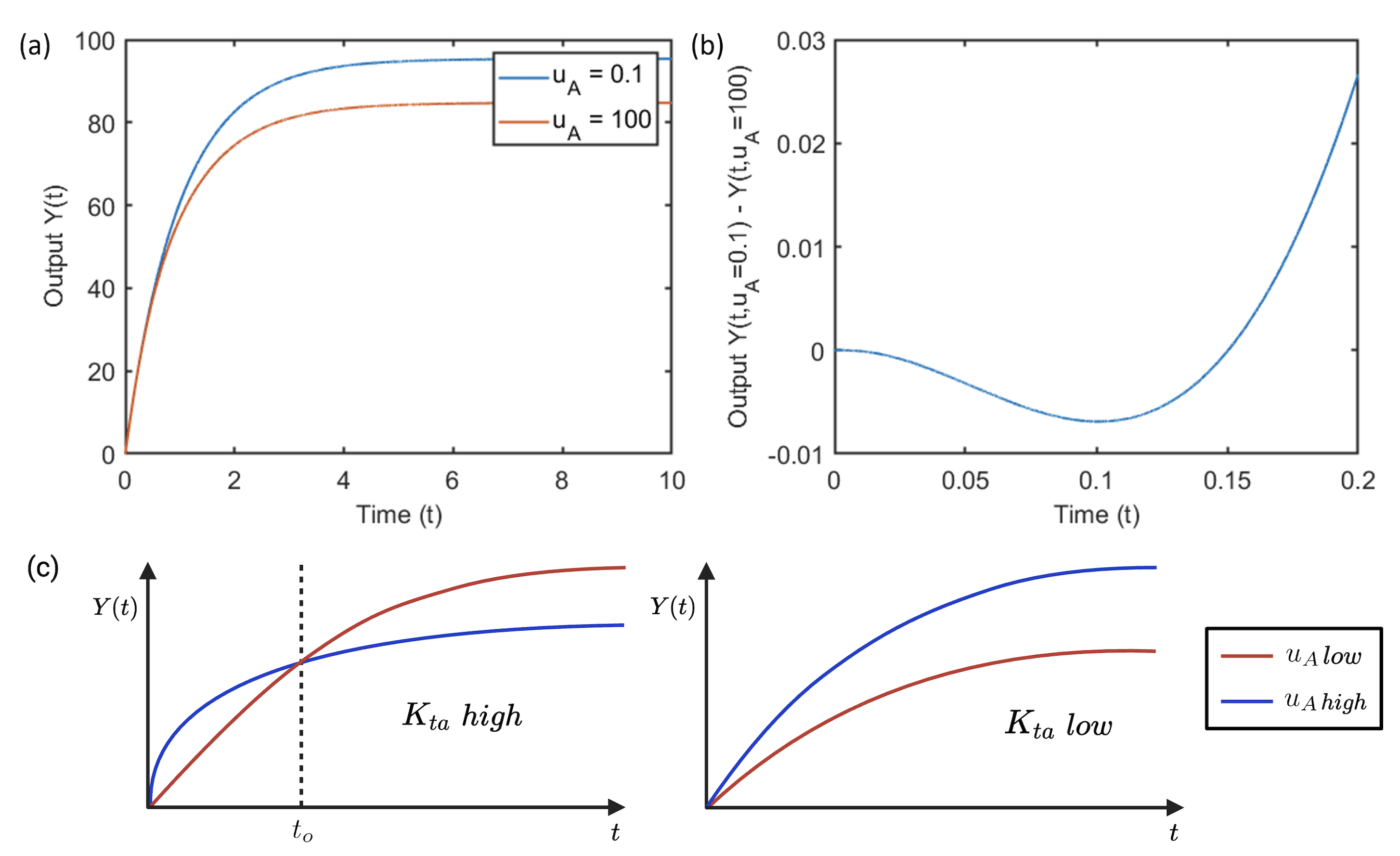
Figure 8: Transient dynamics is devoid of paradoxical effects. Time series of the (a) concentration of the output protein $Y(t)$ for $u_{A}=0.1$ and $u_{A}=100$, and (b) difference between the output levels of the protein $Y(t,u_{A}=0.1)-Y(t,u_{A}=100)$, for $K_{ta}=50$. Generally, one may describe the existence for initial crossing times as depicted in (c). The parameter values are same as Figure 7

Figure 8 displays the flip in the behavior of the synthetic circuit after an initial transient to exhibit the paradoxical effect. The time series of $Y(t)$ shows the existence of the paradoxical effect, where the output level for $u_{A}=0.1$ is higher than that of $u_{A}=100$. However, taking a closer look at the data, the effect emerges after a finite duration of time. This is shown by plotting the difference between the output levels for $u_{A}=0.1$ and $u_{A}=100$ in Figure 8(b). We see that $t<t_{o}$ (where $t_{o}>0$ is a threshold value of time for different combinations of inputs, $t_{0}\approx 0.15$ for $u_{A}=0.1$ and $u_{A}=100$), $Y(u_{A}=100)>Y(u_{A}=0.1)$, i.e., an increase in the activator increases the output protein levels and therefore no paradoxical effect. Whereas for $t>t_{o}$, $Y(u_{A}=100)<Y(u_{A}=0.1)$, i.e., an increase in the activator decreases the output protein levels and therefore exhibits the paradoxical effect. Hence, the output protein levels of the circuit with low input values (say $u_{A}=0.1$) start at $t=0$ with a lower initial growth rate, cross the trajectory of an intermediate input level (say $u_{A}=100$), before reaching a higher steady state value than the intermediate one, as depicted in Figure 8(c). The parameters used for the numerical simulations are somewhat arbitrary, therefore the magnitude of the effects and the timescales could be expected to be different in practice.

III-C Increasing decoy sites increases the output

The paradoxical effect is also portrayed by varying the levels of decoy sites in the system.

Theorem 3

The proposed synthetic circuit exhibits the paradoxical effect given by:

$$\frac{\mathrm{d}\bar{Y}}{\mathrm{d}D_{{\textsc{t}}}}>0\qquad\text{as}\qquad K_{ta}\rightarrow\infty$$

where $\bar{Y}$ is the steady-state levels of the protein when other inputs ($u_{R},u_{A}$) and parameters ($T_{{\textsc{t}}}$, reaction rate constants) are kept constant.

Proof.  Under the limit of $K_{ta}\rightarrow\infty,\overline{T_{A}}\rightarrow\infty$, and from equation (6), the steady-state levels of the output protein is:

$$\overline{Y}=\frac{\beta\overline{T}}{\gamma}\implies\frac{\mathrm{d}\overline{Y}}{\mathrm{d}D_{{\textsc{t}}}}=\frac{\beta}{\gamma}\frac{\mathrm{d}\overline{T}}{\mathrm{d}D_{{\textsc{t}}}}.$$

The conservation at steady state shown in equations (11)-(13) becomes:

$$\overline{A_{{\textsc{t}}}} =\overline{A}+\frac{\overline{D}\overline{A}}{K_{da}}, \overline{R_{{\textsc{t}}}}= \overline{R}+\frac{\overline{T}\overline{R}}{K_{tr}}+\frac{\overline{D}\overline{R}}{K_{dr}},$$ (19)

$$\overline{T_{{\textsc{t}}}} =\overline{T}+\frac{\overline{T}\overline{R}}{K_{tr}}, \overline{D_{{\textsc{t}}}}= \overline{D}+\frac{\overline{D}\overline{A}}{K_{da}}+\frac{\overline{D}\overline{R}}{K_{dr}},$$ (20)

$$\therefore\overline{A} =\frac{\overline{A_{{\textsc{t}}}}}{1+\frac{\overline{D}}{K_{da}}}, \overline{R}= \frac{\overline{R_{{\textsc{t}}}}}{1+\frac{\overline{D}}{K_{dr}}+\frac{\overline{T}}{K_{tr}}}.$$ (21)

Substituting equations (21) in (20), and differentiating with respect to $D_{{\textsc{t}}}$, we get:

$$C_{1}\frac{\mathrm{d}\overline{D}}{\mathrm{d}D_{{\textsc{t}}}}=C_{2}+C_{3}\frac{\mathrm{d}\overline{T}}{\mathrm{d}D_{{\textsc{t}}}}\quad\text{and}\quad C_{4}\frac{\mathrm{d}\overline{T}}{\mathrm{d}D_{{\textsc{t}}}}=C_{5}\frac{\mathrm{d}\overline{D}}{\mathrm{d}D_{{\textsc{t}}}},$$

where

$$C_{1} =1-\frac{D_{{\textsc{t}}}}{\left(1+\frac{\overline{R}}{K_{dr}}+\frac{\overline{A}}{K_{da}}\right)^{2}}\left[\frac{\overline{R}^{2}}{K_{dr}^{2}R_{{\textsc{t}}}}+\frac{\overline{A}^{2}}{K_{da}^{2}A_{{\textsc{t}}}}\right]>0,$$

$$C_{2} =\frac{1}{1+\frac{\overline{R}}{K_{dr}}+\frac{\overline{A}}{K_{da}}}>0,$$

$$C_{3} =\frac{D_{{\textsc{t}}}}{\left(1+\frac{\overline{R}}{K_{dr}}+\frac{\overline{A}}{K_{da}}\right)^{2}}\frac{\overline{R}^{2}}{K_{dr}K_{tr}R_{{\textsc{t}}}}>0,$$

$$C_{4} =1-\frac{\overline{T}^{2}\overline{R}^{2}}{K_{tr}^{2}T_{{\textsc{t}}}R_{{\textsc{t}}}}>0\quad\text{and}\quad C_{5}=\frac{\overline{T}^{2}\overline{R}^{2}}{K_{tr}K_{dr}T_{{\textsc{t}}}R_{{\textsc{t}}}}>0.$$

Eliminating $\frac{\mathrm{d}\overline{D}}{\mathrm{d}D_{{\textsc{t}}}}$, we get:

$$\frac{\mathrm{d}\overline{T}}{\mathrm{d}D_{{\textsc{t}}}}=\frac{C_{2}}{\left(\frac{C_{1}C_{4}}{C_{5}}-C_{3}\right)}>0,\quad\text{as}\quad\frac{C_{1}C_{4}}{C_{5}}-C_{3}>0.$$

Therefore, under the limit of $K_{ta}\rightarrow\infty$,

$$\frac{\mathrm{d}\overline{D}}{\mathrm{d}D_{{\textsc{t}}}}>0.$$  

Figure 7 (b) shows the variation of steady-state output levels ($\overline{Y}$) as a function of decoy sites ($D_{{\textsc{t}}}$) for different values of $K_{ta}$. For $K_{ta}=0.1$, we observe the expected behavior of the output levels decreasing as the amount of decoy sites increases. On the contrary, the behavior flips for higher $K_{ta}$ values showing the exhibition of the paradoxical effect. In the two-parameter bifurcation plots in Figure 7 (c), we see that for high $K_{ta}$ value, the paradoxical affect is observed for all values of $u_{A}$. Increasing the amount of $D_{\textsc{t}}$, increases the output concentration. However, the value of $D_{\textsc{t}}$ after which the system moves to an activated state depends on the value of $u_{A}$. Therefore, the onset of the effect can be controlled using the activator levels. In the case of low $K_{ta}$ value in Figure 7 (d), we see that increasing $D_{{\textsc{t}}}$, decreases the protein levels irrespective of the value of $u_{A}$.

Next, we examine the onset of the paradoxical effect in a similar manner as section III-B.

Theorem 4

Considering the proposed circuit, with $Y$ is a function of $t$ and $D_{{\textsc{t}}}$, i.e. $Y(t,D_{{\textsc{t}}})$, we have:

$$\partial_{D_{{\textsc{t}}}}Y(0,D_{{\textsc{t}}})=\partial_{D_{{\textsc{t}}}}\dot{Y}(0,D_{{\textsc{t}}})=\partial_{D_{{\textsc{t}}}}\ddot{Y}(0,D_{{\textsc{t}}})=0,$$

Then,

$$\partial_{D_{{\textsc{t}}}}{\dddot{Y}}(t,D_{{\textsc{t}}})<0\text{ when }At^{+}_{a}d^{+}_{a}(\kappa-\beta)>Rt^{+}_{r}d^{+}_{r}(\beta)$$

and

$$\partial_{D_{{\textsc{t}}}}\dddot{Y}(t,D_{{\textsc{t}}})>0\text{ when }At^{+}_{a}d^{+}_{a}(\kappa-\beta)<Rt^{+}_{r}d^{+}_{r}(\beta)$$

for small enough $t$.

Proof.  Similarly from Theorem 2, we can repeatedly take Lie derivatives to find dependence on $D_{{\textsc{t}}}$ in the Taylor expansion from equation (18). It follows from equations (16) and (17), that the first and second order terms in equation (18) do not have dependence on $D_{{\textsc{t}}}$.

Looking at the second lie derivative, note that only differentiating $D_{A}$ or $D_{R}$ would give terms involving $D_{T}$. After differentiating the third Lie derivative and only keeping track of these terms, we will see a term of the form

$$D_{{\textsc{t}}}(-(\kappa-\beta)t_{a}^{+}(T_{{\textsc{t}}}-T_{R}-T_{A})d_{a}^{+}(A_{{\textsc{t}}}-D_{A}-T_{A})\,+\\ \beta t_{r}^{+}(T_{{\textsc{t}}}-T_{R}-T_{A})d_{r}^{+}(R_{{\textsc{t}}}-D_{R}-T_{R}))\\ =D_{{\textsc{t}}}(-(\kappa-\beta)t_{a}^{+}d_{a}^{+}TA+\beta t_{r}^{+}d_{r}^{+}TR)$$ (22)

From this term we can observe that if

$$At^{+}_{a}d^{+}_{a}(\kappa-\beta)<Rt^{+}_{r}d^{+}_{r}(\beta)$$

Then for small time, increases in $D_{{\textsc{t}}}$ lead to increases in $Y$, and if

$$At^{+}_{a}d^{+}_{a}(\kappa-\beta)>Rt^{+}_{r}d^{+}_{r}(\beta)$$

for small times, increases in $D_{{\textsc{t}}}$ lead to decreases in $Y$.  

IV Additional system properties

Claim 1

The proposed synthetic circuit with the reaction network given by equations (1) admits bounded trajectories.

Proof.  Note we have conservation laws $D+D_{A}+D_{R}=D_{{\textsc{t}}}$ and $T+T_{A}+T_{R}=T_{{\textsc{t}}}$, which implies all these quantities are bounded above by $e=\max(D_{{\textsc{t}}},T_{{\textsc{t}}})$. Similarly:

$$\dot{A} =-\delta A+u_{a}-d_{a}^{+}AD-t_{a}^{+}AT+d_{a}^{-}D_{A}+t_{a}^{-}T_{A}$$

$$\leq-\delta A-d_{a}^{+}AD-t_{a}^{+}AT+(d_{a}^{-}+t_{a}^{-})e+u_{a}.$$

Thus for large enough values of $A$, the above expression will be negative, therefore $A$ is bounded from above. The same reasoning applies to $R$:

$$\dot{R}=-\delta R+u_{R}-d_{r}^{+}RD-t_{r}^{+}RT+d_{r}^{-}D_{R}+t_{r}^{-}T_{R}$$

$$\leq-\delta R+(d_{r}^{-}+t_{r}^{-})e+u_{R}$$

In particular, the polytope described by the equations:

$$D+D_{A}+D_{R}=D_{{\textsc{t}}},\qquad T+T_{A}+T_{R}=T_{{\textsc{t}}},$$

$$A\leq\frac{(d_{a}^{-}+t_{a}^{-})e+u_{a}}{\delta},\qquad R\leq\frac{(d_{r}^{-}+t_{r}^{-})e+u_{R}}{\delta},$$

$$A,R,D_{A},D_{R},T_{A},T_{R},D,T\geq 0$$

is invariant under our vector field, and thus our trajectories are bounded.  

Claim 2

The reaction network has an equilibrium.

Proof.  From Claim 1, there is a compact and convex set of values of our system species $\{T_{R},T_{A},D_{R},D_{A},Y,A_{{\textsc{t}}},R_{{\textsc{t}}}\}$ that is closed under the time evolution of our system. By Brouwer’s fixed point theorem for every $t\geq 0$ we have the time evolution $\phi_{t}$ has a fixed point $\bar{x}_{t}$. Take a sequence of $t_{n}\rightarrow 0$, the sequence $\bar{x}_{t_{n}}$ has a limit point $\bar{x}$. If $\bar{x}$ was not an equilibrium, then for small $t$ it would not be a fixed point for $\phi_{t}$, which is a contradiction. Thus $\bar{x}$ is an equilibrium of our vector field.  

This theorem applies to our system, and implies that our system has at least one equilibrium. Next we will note that this equilibrium must be in fact unique.

In order to know that an equilibrium is in fact the unique equlibrium of the system, we can use the notion of injectivity. We say the system is injective, as in [12], if for all possible kinetic parameters the system $\dot{x}=f(x,p)$ is such that $f(x,p)$ is an injective function, no matter the choice of $p$. If this is true, it implies $f(x,p)=0$ has at most one solution (i.e., we have at most one equilibrium).

Claim 3

The proposed synthetic circuit is injective.

Proof.  Using the conservation laws, $T_{{\textsc{t}}}=T+T_{A}+T_{R}$ and $D_{{\textsc{t}}}=D+D_{A}+D_{R}$, we can form the “extended rate function” by simply replacing the dynamics for $\dot{T}$ and $\dot{D}$ with our conservation laws. We can then take the determinant of the Jacobian of this modified rate function and verify all its terms are positive, which implies injectivity by Theorem 8.1 in [12]. Mathematica code for this computation can be found in the appendix. Inspection of the output confirms the Jacobian is always nonzero and thus our system is injective.  

V Discussion

Starting from a hypothesis concerning the role of off-target binding in explaining paradoxical behaviors of activators and repressors observed experimentally in cancer cell culture experiments, this paper proposed a synthetic biology experiment to reproduce these behaviors in a controlled situation. A mathematical analysis was used to identify appropriate parameter regimes, and theoretical results were obtained. Work is ongoing to build the appropriate synthetic constructs and perform confirmatory experiments. Model-driven experiments are being performed using CRISPRa as the activator and CRISPRi as the repressor.

Acknowledgements

The authors wish to thank Dr. Polly Yu for very useful discussions and suggestions regarding the use of the injectivity property.

-A Calculating the derivatives $\frac{dR}{dA_{{\textsc{t}}}},\frac{dA}{dA_{{\textsc{t}}}}$ and thereby $\frac{dY}{dA_{{\textsc{t}}}}$

Using equation (11) - (13),

$$\overline{R_{{\textsc{t}}}}-\overline{R}+\frac{\overline{T}\overline{R}}{K_{tr}}+\frac{\overline{D}\overline{R}}{K_{dr}}=0$$

Taking the derivative with respect to $A_{{\textsc{t}}}$:

$$\frac{dR}{dA_{{\textsc{t}}}}(1+\frac{D_{{\textsc{t}}}}{K_{dr}(1+\frac{R}{K_{dr}}+\frac{A}{K_{da}})}+ \frac{T_{{\textsc{t}}}}{K_{tr}(1+\frac{R}{K_{tr}}+\frac{A}{K_{ta}})})$$

$$-\frac{RD_{{\textsc{t}}}}{K_{dr}(O_{D})^{2}}(\frac{1}{K_{dr}}\frac{dR}{dA_{{\textsc{t}}}}+\frac{1}{K_{da}}\frac{dA}{dA_{{\textsc{t}}}})-\frac{RT_{{\textsc{t}}}}{K_{tr}(O_{T})^{2}}(\frac{1}{K_{tr}}\frac{dR}{dA_{{\textsc{t}}}}+\frac{1}{K_{ta}}\frac{dA}{dA_{{\textsc{t}}}})=0$$

where

$$O_{D}=1+\frac{D_{{\textsc{t}}}}{K_{dr}(1+\frac{R}{K_{dr}}+\frac{A}{K_{da}}}\qquad\text{ and }\qquad O_{t}=1+\frac{T_{tot}}{K_{dr}(1+\frac{R}{K_{dr}}+\frac{A}{K_{da}}})$$

After reorganizing, we get:

$$\frac{dR}{dA_{{\textsc{t}}}}=\frac{(\frac{RD_{{\textsc{t}}}}{K_{da}K_{dr}(1+\frac{R}{K_{dr}}+\frac{A}{K_{da}})^{2}}+\frac{RT_{{\textsc{t}}}}{K_{ta}K_{tr}(1+\frac{R}{K_{tr}}+\frac{A}{K_{ta}})^{2}})\frac{dA}{dA_{{\textsc{t}}}}}{(1+\frac{D_{{\textsc{t}}}}{K_{dr}(1+\frac{R}{K_{dr}}+\frac{A}{K_{da}})}(1-\frac{\frac{R}{K_{dr}}}{(1+\frac{R}{K_{dr}}+\frac{A}{K_{da}})})\frac{T_{{\textsc{t}}}}{K_{tr}(1+\frac{R}{K_{tr}}+\frac{A}{K_{ta}})}(1-\frac{\frac{R}{K_{tr}}}{(1+\frac{R}{K_{tr}}+\frac{A}{K_{ta}})}))}$$

Doing a similar approach on the conservation law for $A_{\textsc{t}}$, we get:

$$\frac{dA}{dA_{{\textsc{t}}}} (1+\frac{D_{{\textsc{t}}}}{K_{da}(1+\frac{R}{K_{dr}}+\frac{A}{K_{da}})}+\frac{T_{{\textsc{t}}}}{K_{ta}(1+\frac{R}{K_{tr}}+\frac{A}{K_{ta}})})$$

$$-\frac{AD_{{\textsc{t}}}}{K_{da}(O_{t})^{2}}(\frac{1}{K_{dr}}\frac{dR}{dA_{{\textsc{t}}}}+\frac{1}{K_{da}}\frac{dA}{dA_{{\textsc{t}}}})-\frac{AT_{{\textsc{t}}}}{K_{ta}(O_{t})^{2}}(\frac{1}{K_{tr}}\frac{dR}{dA_{{\textsc{t}}}}+\frac{1}{K_{ta}}\frac{dA}{dA_{{\textsc{t}}}})=1$$

Rearranging, we get:

$$\frac{dA}{dA_{{\textsc{t}}}}(1+\frac{D_{{\textsc{t}}}}{K_{da}(1+\frac{R}{K_{dr}}+\frac{A}{K_{da}})} (1-\frac{\frac{A}{K_{da}}}{1+\frac{R}{K_{dr}}+\frac{A}{K_{da}}})+\frac{T_{{\textsc{t}}}}{K_{ta}(1+\frac{R}{K_{tr}}+\frac{A}{K_{ta}})}(1-\frac{\frac{A}{K_{ta}}}{1+\frac{R}{K_{tr}}+\frac{A}{K_{ta}}}))$$

$$=1+(\frac{AD_{{\textsc{t}}}}{K_{da}K_{dr}(1+\frac{R}{K_{dr}}+\frac{A}{K_{da}})^{2}}+\frac{AT_{{\textsc{t}}}}{K_{ta}K_{tr}(1+\frac{R}{K_{tr}}+\frac{A}{K_{ta}})^{2}})\frac{dR}{dA_{{\textsc{t}}}}$$

Substituting $\frac{dR}{dA_{{\textsc{t}}}}$:

$$\frac{dA}{dA_{{\textsc{t}}}}=\frac{(1+\frac{D_{{\textsc{t}}}(1+\frac{A}{K_{da}})}{K_{dr}(1+\frac{R}{K_{dr}}+\frac{A}{K_{da}})^{2}}+\frac{T_{{\textsc{t}}}(1+{\frac{A}{K_{ta}}})}{K_{tr}(1+\frac{R}{K_{tr}}+\frac{A}{K_{ta}})^{2}})}{\text{De}}$$

Where:

De $$=1+\frac{D_{{\textsc{t}}}(1+\frac{A}{K_{da}})}{K_{dr}(1+\frac{R}{K_{dr}}+\frac{A}{K_{da}})^{2}}+\frac{T_{{\textsc{t}}}(1+{\frac{A}{K_{ta}}})}{K_{tr}(1+\frac{R}{K_{tr}}+\frac{A}{K_{ta}})^{2}}+\frac{D_{{\textsc{t}}}(1+\frac{R}{K_{dr}})}{K_{da}(1+\frac{R}{K_{dr}}+\frac{A}{K_{da}})^{2}}$$

$$\qquad\qquad+\frac{D_{{\textsc{t}}}^{2}}{K_{dr}K_{da}(1+\frac{R}{K_{dr}}+\frac{A}{K_{da}})^{4}}(1+\frac{R}{K_{dr}}+\frac{A}{K_{da}})+\frac{D_{{\textsc{t}}}(1+\frac{R}{K_{dr}}+\frac{A}{K_{ta}})T_{{\textsc{t}}}}{K_{da}(1+\frac{R}{K_{dr}}+\frac{A}{K_{da}})^{2}K_{tr}(1+\frac{R}{K_{tr}}+\frac{A}{K_{ta}})^{2}}$$

$$\qquad\qquad+\frac{T_{{\textsc{t}}}(1+\frac{R}{K_{tr}})}{K_{ta}(1+\frac{R}{K_{tr}}+\frac{A}{K_{ta}})^{2}}+\frac{T_{{\textsc{t}}}(1+\frac{R}{K_{tr}}+\frac{A}{K_{da}})D_{{\textsc{t}}}}{K_{ta}(1+\frac{R}{K_{tr}}+\frac{A}{K_{ta}})^{2}K_{dr}(1+\frac{R}{K_{dr}}+\frac{A}{K_{da}})^{2}}+\frac{T_{{\textsc{t}}}^{2}(1+\frac{R}{K_{tr}}+\frac{A}{K_{ta}})}{K_{tr}K_{ta}(1+\frac{R}{K_{tr}}+\frac{A}{K_{ta}})^{4}}$$

Now that we have explicit equations for the derivatives, $\frac{dA}{dA_{{\textsc{t}}}}$ and $\frac{dR}{dA_{{\textsc{t}}}}$, we look at $\frac{dY}{dA_{{\textsc{t}}}}$:

$$\frac{dY}{dA_{{\textsc{t}}}} =\frac{1}{\gamma}(\frac{\kappa}{K_{ta}}A+\beta)\frac{dT}{dA_{{\textsc{t}}}}+\frac{1}{\gamma}\frac{\kappa T}{K_{ta}}\frac{dA}{dA_{{\textsc{t}}}}$$

$$=\frac{1}{\gamma}\frac{\kappa T}{K_{ta}}\frac{dA}{dA_{{\textsc{t}}}}-\frac{1}{\gamma}(\frac{\kappa}{K_{ta}}A+\beta)\frac{T_{{\textsc{t}}}}{(1+\frac{R}{K_{tr}}+\frac{A}{K_{ta}})^{2}}(\frac{1}{K_{tr}}\frac{dR}{dA_{{\textsc{t}}}}+\frac{1}{K_{ta}}\frac{dA}{dA_{{\textsc{t}}}})$$

$$=\frac{1}{\gamma\text{De}}(\frac{\kappa T_{{\textsc{t}}}}{K_{ta}(1+\frac{R}{K_{tr}}+\frac{A}{K_{ta}})}(1+\frac{D_{{\textsc{t}}}(1+\frac{A}{K_{da}})}{K_{dr}(1+\frac{R}{K_{dr}}+\frac{A}{K_{da}})^{2}}+\frac{T_{{\textsc{t}}}(1+\frac{A}{K_{ta}})}{K_{tr}(1+\frac{R}{K_{tr}}+\frac{A}{K_{ta}})^{2}})$$

$$\qquad\qquad-(\frac{\kappa}{K_{ta}}A+\beta)\frac{T_{{\textsc{t}}}}{(1+\frac{R}{K_{tr}}+\frac{A}{K_{ta}})^{2}}(\frac{1}{K_{tr}}(\frac{RD_{{\textsc{t}}}}{K_{da}K_{dr}(1+\frac{R}{K_{dr}}+\frac{A}{K_{da}})^{2}}+\frac{RT_{{\textsc{t}}}}{K_{ta}K_{tr}(1+\frac{R}{K_{tr}}+\frac{A}{K_{ta}})^{2}})$$

$$\qquad\qquad+\frac{1}{K_{ta}}(1+\frac{D_{{\textsc{t}}}(1+\frac{A}{K_{da}})}{K_{dr}(1+\frac{R}{K_{dr}}+\frac{A}{K_{da}})^{2}})))$$

$$=\frac{1}{\gamma\text{De}}(\frac{\kappa T_{{\textsc{t}}}}{K_{ta}(1+\frac{R}{K_{ta}}+\frac{A}{K_{ta}})^{2}}(1+\frac{D_{{\textsc{t}}}(1+\frac{A}{K_{da}})}{K_{dr}(1+\frac{R}{K_{dr}}+\frac{A}{K_{da}})^{2}}+\frac{T_{{\textsc{t}}}(1+\frac{A}{K_{ta}})}{K_{tr}(1+\frac{R}{K_{tr}}+\frac{A}{K_{ta}})^{2}})(1+\frac{R}{K_{tr}})$$

$$\qquad\qquad-\frac{A}{K_{tr}}(\frac{\kappa}{K_{ta}}A+\beta)\frac{T_{{\textsc{t}}}}{(1+\frac{R}{K_{tr}}+\frac{A}{K_{ta}})^{2}}\frac{1}{K_{tr}}(\frac{RD_{{\textsc{t}}}}{K_{da}K_{dr}(1+\frac{R}{K_{dr}}+\frac{A}{K_{da}})^{2}}+\frac{RT_{{\textsc{t}}}}{K_{ta}K_{tr}(1+\frac{R}{K_{tr}}+\frac{A}{K_{ta}})^{2}})$$

$$\qquad\qquad-\frac{\beta T_{{\textsc{t}}}}{(1+\frac{R}{K_{tr}}+\frac{A}{K_{ta}})^{2}}\frac{1}{K_{ta}}(1+\frac{D_{{\textsc{t}}}(1+\frac{A}{K_{da}})}{K_{dr}(1+\frac{R}{K_{dr}}+\frac{A}{K_{da}})^{2}}+\frac{T_{{\textsc{t}}}(1+\frac{A}{K_{ta}})}{K_{tr}(1+\frac{R}{K_{tr}}+\frac{A}{K_{ta}})^{2}}))$$

Therefore:

$$\frac{dY}{dA_{{\textsc{t}}}}=\frac{1}{\gamma\text{De}}\frac{T_{{\textsc{t}}}}{(1+\frac{R}{K_{tr}}+\frac{A}{K_{ta}})}(\frac{\kappa}{K_{ta}}(1+\frac{R}{K_{tr}}+\frac{D_{{\textsc{t}}}(1+\frac{A}{K_{da}}+\frac{R}{K_{tr}})}{K_{dr}(1+\frac{R}{K_{dr}}+\frac{A}{K_{da}})^{2}}+\frac{T_{{\textsc{t}}}}{K_{tr}(1+\frac{R}{K_{tr}}+\frac{A}{K_{ta}})})$$

$$\qquad\qquad-\beta(\frac{R\frac{D_{{\textsc{t}}}}{K_{tr}}}{K_{da}K_{dr}(1+\frac{R}{K_{dr}}+\frac{A}{K_{da}})^{2}}+\frac{R\frac{T_{{\textsc{t}}}}{K_{tr}}}{K_{ta}K_{tr}(1+\frac{R}{K_{tr}}+\frac{A}{K_{ta}})^{2}}+\frac{1}{K_{ta}}$$

$$\qquad\qquad+\frac{D_{{\textsc{t}}}(1+\frac{A}{K_{da}})}{K_{ta}K_{dr}(1+\frac{R}{K_{dr}}+\frac{A}{K_{da}})^{2}}\frac{T_{{\textsc{t}}}(1+\frac{A}{K_{ta}})}{K_{ta}K_{tr}(1+\frac{R}{K_{tr}}+\frac{A}{K_{ta}})^{2}}))$$

Comparing the above equation with equation (15):

$$g_{1}(\overline{A},\overline{R}) =\frac{1}{\gamma\text{De}}\frac{T_{{\textsc{t}}}}{(1+\frac{R}{K_{tr}}+\frac{A}{K_{ta}})}$$

$$g_{3}(\overline{A}),\overline{R} =(\kappa(1+\frac{R}{K_{tr}}+\frac{D_{{\textsc{t}}}(1+\frac{A}{K_{da}}+\frac{R}{K_{tr}})}{K_{dr}(1+\frac{R}{K_{dr}}+\frac{A}{K_{da}})^{2}}+\frac{T_{{\textsc{t}}}}{K_{tr}(1+\frac{R}{K_{tr}}+\frac{A}{K_{ta}})})$$

-B Mathematica Code

Listing 1: Code for injectivity proof

⬇

1Adot[A_, R_, Da_, Dr_, Ta_, Tr_, t_, d_] = -k1 A*D + k2 Da - k5 A*T + k6 Ta - k9 A;

2

3Rdot[A_, R_, Da_, Dr_, Ta_, Tr_, T_, D_] = -k3 R*D + k4 Dr - k7 R*T + k8 Tr - k10 R;

4

5Dadot[A_, R_, Da_, Dr_, Ta_, Tr_, T_, D_] = k1 A*D - k2 Da - k13 Da ;

6

7Drdot[A_, R_, Da_, Dr_, Ta_, Tr_, T_, D_] = k3 R*D - k4 Dr - k14 Dr ;

8

9Tadot[A_, R_, Da_, Dr_, Ta_, Tr_, T_, D_] = k5 A*T - k6 Ta - k11 Ta ;

10

11Trdot[A_, R_, Da_, Dr_, Ta_, Tr_, T_, D_] = k7 R*T - k8 Tr - k12 Tr ;

12

13Tdot[A_, R_, Da_, Dr_, Ta_, Tr_, T_, D_] = -k5 A*T + k6 Ta - k7 R*T + k8 Tr + k11 Ta + k12 Tr ;

14

15Ddot[A_, R_, Da_, Dr_, Ta_, Tr_, T_, D_] = -k1 A*D + k2 Da - k3 R*D + k4 Dr + k13 Da + k14 Dr ;

16

17ConsvT[A_, R_, Da_, Dr_, Ta_, Tr_, T_, D_] = Tr + Ta + T;

18

19ConsvD[A_, R_, Da_, Dr_, Ta_, Tr_, T_, D_] = Dr + Da + D ;

20

21modRHS = {Adot[A, R, Da, Dr, Ta, Tr, T, D],

22 Rdot[A, R, Da, Dr, Ta, Tr, T, D],

23 Dadot[A, R, Da, Dr, Ta, Tr, T, D],

24 Drdot[A, R, Da, Dr, Ta, Tr, T, D],

25 Tadot[A, R, Da, Dr, Ta, Tr, T, D],

26 Trdot[A, R, Da, Dr, Ta, Tr, T, D],

27 ConsvT[A, R, Da, Dr, Ta, Tr, T, D],

28 ConsvD[A, R, Da, Dr, Ta, Tr, T, D]

29 };

30

31Grad[modRHS, {A, R, Da, Dr, Ta, Tr, T, D}] // Det

References

• [1] D. Del Vecchio, A. Ninfa, and E. Sontag, “Modular cell biology: Retroactivity and insulation,” Molecular Systems Biology, vol. 4, p. 161, 2008.
• [2] S. Cardinale and A. P. Arkin, “Contextualizing context for synthetic biology - identifying causes of failure of synthetic biological systems,” Biotechnology Journal, vol. 7, no. 7, pp. 856–866, 2012.
• [3] N. Shakiba, R. D. Jones, R. Weiss, and D. Del Vecchio, “Context-aware synthetic biology by controller design: Engineering the mammalian cell,” Cell Systems, vol. 12, no. 6, pp. 561–592, 2021. [Online]. Available: https://www.sciencedirect.com/science/article/pii/S2405471221001976
• [4] M. Al-Radhawi, D. Del Vecchio, and E. Sontag, “Identifying competition phenotypes in synthetic biochemical circuits,” IEEE Control Systems Letters, vol. 7, pp. 211–216, 2023.
• [5] D. Del Vecchio, “Modularity, context-dependence, and insulation in engineered biological circuits,” Trends in Biotechnology, vol. 33, no. 2, pp. 111–119, 2015, special Issue: Manifesting Synthetic Biology. [Online]. Available: https://www.sciencedirect.com/science/article/pii/S0167779914002388
• [6] A. Stone, A. Youssef, S. Rijal, R. Zhang, and X.-J. Tian, “Context-dependent redesign of robust synthetic gene circuits,” Trends in Biotechnology, 2024. [Online]. Available: https://www.sciencedirect.com/science/article/pii/S0167779924000039
• [7] D. Del Vecchio, Y. Qian, R. Murray, and E. Sontag, “Future systems and control research in synthetic biology,” Annual Reviews in Control, vol. 45, pp. 5–17, 2018.
• [8] M. Al-Radhawi, S. Tripathi, Y. Zhang, E. Sontag, and H. Levine, “Epigenetic factor competition reshapes the EMT landscape,” Proc Natl Acad Sci USA, vol. 119, p. e2210844119, 2022.
• [9] B. Schuettengruber, H.-M. Bourbon, L. Di Croce, and G. Cavalli, “Genome regulation by polycomb and trithorax: 70 years and counting,” Cell, vol. 171, no. 1, pp. 34–57, 2017.
• [10] Y. Zhang, J. L. Donaher, S. Das, X. Li, F. Reinhardt, J. A. Krall, A. W. Lambert, P. Thiru, H. R. Keys, M. Khan, et al., “Genome-wide CRISPR screen identifies PRC2 and KMT2D-COMPASS as regulators of distinct EMT trajectories that contribute differentially to metastasis,” Nature cell biology, vol. 24, no. 4, pp. 554–564, 2022.
• [11] D. Del Vecchio and R. M. Murray, Biomolecular Feedback Systems.   Princeton University Press, 2014.
• [12] C. Wiuf and E. Feliu, “Power-law kinetics and determinant criteria for the preclusion of multistationarity in networks of interacting species,” SIAM Journal on Applied Dynamical Systems, vol. 12, no. 4, pp. 1685–1721, 2013. [Online]. Available: https://doi.org/10.1137/120873388