A Kinetic Scheme based on Positivity Preservation with Exact Shock Capture

Abstract

In this paper, we describe a kinetic model with flexible velocities which are set to satisfy positivity preservation conditions for the Euler equations. Our kinetic model in 1D comprises of two velocities, and both the asymmetrical and the symmetrical models are utilized. Switching between the two models is done based on our own version of kinetic relative entropy and an additional criterion, to ensure an accurate, entropic and robust scheme. In 2D, we describe a novel three-velocity kinetic model, defined to ensure a locally 1D formulation for the resulting macroscopic normal flux. For first order accuracy, we also obtain a limit on the time step which ensures positivity preservation. The resulting numerical scheme captures grid-aligned steady shocks exactly. Several benchmark compressible flow test cases are solved in 1D and 2D to demonstrate the efficacy of the proposed solver.

[1]organization=Research Scholar, Department of Aerospace Engineering, Indian Institute of Science,city=Bangalore, country=India

[2]organization=Department of Aerospace Engineering, Indian Institute of Science,city=Bangalore, country=India

1 Introduction

Among the different types of numerical schemes for solving the hyperbolic Euler equations, kinetic schemes stand out as they do not directly discretize the Euler equations. Instead, kinetic schemes start by discretizing the Boltzmann equation, which is the governing equation at the kinetic level. Suitable moments of the Boltzmann equation give us the macroscopic conservation laws and this strategy leads to efficient kinetic or Boltzmann schemes. Some of the well known early generation kinetic schemes are described in [1, 2, 3, 4, 5, 6, 7, 8, 9, 10, 11]. While there are many more in this category, the schemes of particular interest is the vector kinetic framework with discrete velocities, developed by Natalini [12] and Aregba-Driollet and Natalini [13]. Shrinath et al. [14] have utilized the conservation form of vector kinetic equations and flexible velocities satisfying Rankine-Hugoniot (R-H) jump conditions at the interface, to develop a low diffusive kinetic scheme. Recently, Shashi Shekhar Roy and S. V. Raghurama Rao [15] have described a kinetic model for which the equilibrium distribution has flexible velocities and ranges of velocities, and its moments are utilized in a vector kinetic framework. The velocities are used to satisfy the R-H conditions, while the ranges of velocities is used to provide additional numerical diffusion in smoothly varying flow regions. For the purpose of identifying smooth flow regions, a novel formulation for relative entropy is also presented. The last two of the above works focus on exact capture of steady discontinuities, which could be enforced in the discretization only in macroscopic schemes before them.

Positivity preservation is another important feature of numerical schemes and refers to the preservation of positivity of density and pressure (or internal energy) at all points and at all later times, given the initial solution with positive density and pressure. It is a desirable feature in numerical schemes, since most schemes fail once negative pressure is encountered. This generally happens at high Mach numbers, in near vacuum conditions, and in the presence of strong gradients in general. In the category of kinetic schemes, Perthame [9] first demonstrated the positivity of density and pressure in his kinetic scheme. Later, Estivalezes and Villedieu [16] showed that the Kinetic Flux Vector splitting scheme[6] preserves the positivity of density and pressure under a CFL-like condition. They also extended the positivity property to second order accuracy for a positivity preserving flux vector splitting scheme. Gressier et al. [17] showed that flux vector splitting schemes like those of van Leer and Steger-Warming are positivity preserving under a CFL-like condition. Thus, to summarize, many flux vector splitting schemes are positivity preserving. But they have an inherent drawback of being very diffusive. In the category of approximate Riemann solvers, positivity preserving was attempted by Einfeldt et al. [18] by imposing bounds on the wave speeds in HLL (Harten-Lax-Leer) scheme. While there are others in this category, more recent work includes that by Parent[19], who has obtained a positivity preserving scheme by modifying the Roe’s scheme such that the coefficient matrices of the discretized equations are positive. However, many of these solvers are dependent strongly on the eigenstructure of the underlying hyperbolic systems. Further, most of the Riemann solvers suffer from drawbacks like admitting entropy-violating solutions, as well as numerical instability issues like odd-even decoupling, carbuncle phenomenon, kinked Mach stems, etc. [20]. Since kinetic schemes are not dependent on the eigenstructure, they become attractive to enforce additional features like positivity and for application to flows with more realistic and complicated equations of state.

In the present work, we describe a kinetic model for the Euler equations with two flexible velocities in 1D, which are set to satisfy the conditions for positivity preservation. Our objective is to obtain a low-diffusive kinetic scheme which is also positivity preserving. Our numerical scheme is not based on the solution of any Riemann problem, and it neither requires the computation of Roe-averages nor is dependent strongly on the eigenstructure. Our 2D formulation describes a novel three-velocity kinetic model, which is defined to ensure that the resulting normal flux at the interface takes a locally one-dimensional form. We use a reconstruction based flux limited approach and a higher order Runge-Kutta method to extend our basic scheme to second order accuracy. Extensive set of benchmark test cases are solved to demonstrate that our numerical scheme is robust, accurate, entropic and free from numerical instability issues. As a final exercise, the basic scheme is extended to the viscous flows and some benchmark viscous problems are solved to demonstrate the ability of our numerical scheme to resolve the associated flow features.

2 Gas-kinetic theory

According to kinetic theory, the dynamics of gases is governed by the Boltzmann equation, given by

$$\frac{\partial f}{\partial t}+\textbf{v}\cdot\frac{\partial f}{\partial\textsl{{x}}}=Q(f)$$ (1)

Here, $f(t,\textbf{x},\textbf{v})$ is the velocity distribution function, v is molecular velocity, and $Q(f)$ is the rate of change of f due to collisions. The linear advection term in Equation (1) describes the temporal and spatial evolution of the molecular velocity distribution function, which moves the state away from equilibrium. The collision term, on the other hand, is non-linear and it drives the distribution function towards equilibrium, vanishing in a limit (better described with the BGK model mentioned later). The equilibrium distribution function given by gas-kinetic theory is the Maxwell-Boltzmann equilibrium distribution, defined by

$$f^{eq}_{Maxwell}=\frac{\rho}{I_{0}}\left(\frac{\beta}{\pi}\right)^{N/2}exp\left(-\beta|\textbf{v}-\textbf{u}|^{2}\right)exp\left(-I/I_{0}\right)$$ (2)

where $\beta$= $\frac{1}{2RT}$, $\textbf{u}(t,\textbf{x})$ is the macroscopic velocity, $N$ is the translational degrees of freedom, $I$ is the internal energy variable corresponding to non-translational degrees of freedom, $I_{0}~{}=~{}\frac{2-N(\gamma-1)}{2(\gamma-1)}RT$ and $\gamma$= $\frac{c_{p}}{c_{v}}$. The combined mass, momentum and total energy of the particles is conserved during collisions. Thus, 1, v and $I+\frac{|\textbf{v}|^{2}}{2}$ are the collisional invariants. By multiplying the Boltzmann equation with the moment vector $\bm{\Psi}=\left[1,v_{1},..,v_{N},I+\frac{|\textbf{v}|^{2}}{2}\right]^{T}$ and integrating w.r.t. v and $I$, i.e., by taking moments, we obtain the macroscopic conservation laws of mass, momentum and energy. Further, under the assumption that $f$ relaxes instantaneously to $f^{eq}$ (justified through operator splitting and the BGK model), the moments of the Boltzmann equation give us the inviscid Euler equations, as follows.

$$\int_{\mathbb{R}^{N}}d\textbf{v}\int_{\mathbb{R}^{+}}dI\ \bm{\Psi}\left(\frac{\partial f}{\partial t}+\frac{\partial(v_{i}f)}{\partial x_{i}}=0,f=f^{eq}\right)\Rightarrow\frac{\partial\textbf{U}}{\partial t}+\frac{\partial\textbf{G}_{i}}{\partial x_{i}}=0$$ (3)

Here, the conserved variable vector U and the inviscid flux vector along $i$ direction, $\textbf{G}_{i}$ for the Euler equations are given by

$$\textbf{U}=\begin{bmatrix}\rho\\ \rho u_{j}\\ \rho E\end{bmatrix},\textbf{G}_{i}=\begin{bmatrix}\rho u_{i}\\ \rho u_{i}u_{j}+p\delta_{ij}\\ (\rho E+p)u_{i}\end{bmatrix},\ E=e+\frac{|\textbf{u}|^{2}}{2},\ e=\frac{p}{(\gamma-1)\rho}$$ (4)

The moment relations can be written as

$$\int_{\mathbb{R}^{N}}d\textbf{v}\int_{\mathbb{R}^{+}}dI\ \bm{\Psi}f=\int_{\mathbb{R}^{N}}d\textbf{v}\int_{\mathbb{R}^{+}}dI\ \bm{\Psi}f^{eq}=\textbf{U}$$ (5a)

$$\int_{\mathbb{R}^{N}}v_{i}d\textbf{v}\int_{\mathbb{R}^{+}}dI\ \bm{\Psi}f^{eq}=\textbf{G}_{i}$$ (5b)

Multiplying the Boltzmann equation by $\ln f$ and taking its moment, we get the kinetic entropy inequality, i.e., the H-theorem

$$\frac{\partial H}{\partial t}+\frac{\partial H_{v,i}}{\partial x_{i}}\leq 0$$ (6)

with

$$\int_{\mathbb{R}^{N}}d\textbf{v}\int_{\mathbb{R}^{+}}dI\ f\ln f=H,$$ (7a)

$$\int_{\mathbb{R}^{N}}v_{i}d\textbf{v}\int_{\mathbb{R}^{+}}dI\ f\ln f=H_{v,i},$$ (7b)

$$\int_{\mathbb{R}^{N}}d\textbf{v}\int_{\mathbb{R}^{+}}dI\ Q(f)\ln f\leq 0$$ (7c)

Next, we introduce a popular simplification to the collision term, called the BGK model [21]. For this model, the collision term is approximated by the following expression.

$$Q(f)=-\frac{1}{\epsilon}\left[f-f^{eq}\right]$$ (8)

Here, $\epsilon$ is the relaxation time. The description of Boltzmann equations up to this point has assumed that molecular velocity is continuous, taking all possible real values. In contrast, in a discrete velocity Boltzmann system, the distribution function is typically a vector, with each of its components satisfying a Boltzmann equation while being advected by a single velocity. The Discrete Velocity Boltzmann-BGK Equations corresponding to the $i^{th}$ macroscopic equation take the following form.

$$\frac{\partial f_{ji}}{\partial t}+\lambda_{jk}\frac{\partial f_{ji}}{\partial x_{k}}=-\frac{1}{\epsilon}\left[f_{ji}-f^{eq}_{ji}\right],\ j=1,..,N_{d},\ k=1,...,N$$ (9)

The number of discrete velocities, $N_{d}$ satisfies the condition, $N_{d}\geq N+1$. The moment relations become

$$\sum^{N_{d}}_{j=1}f_{ji}=\sum^{N_{d}}_{j=1}f^{eq}_{ji}=U_{i},\ \sum^{N_{d}}_{j=1}\lambda_{jk}f^{eq}_{ji}=(G_{k})_{i}$$ (10)

Thus, in a discrete kinetic framework, the moment relations get simplified, as complex integrals are replaced by simple summations. As a consequence, the equilibrium distributions often become simple linear combinations of the conserved variable vector and inviscid flux vectors. The work in this paper is based on further developments based on the flexible velocity framework introduced in [14, 15].

3 Kinetic model for 1D Euler Equations

In the present work, we are modeling only in the velocity $v$ space. Therefore, we introduce the following truncated equilibrium distributions by integrating w.r.t. the internal energy variable $I$.

$$\breve{f}^{eq}=\int^{\infty}_{0}\ f^{eq}dI,\ \ \hat{f}^{eq}_{i}=\Psi_{i}\breve{f}^{eq}$$ (11)

Then, the moment relations in 1-D become

$$U_{i}=\int_{-\infty}^{\infty}dv\ \Psi_{i}\breve{f}^{eq}=\int_{-\infty}^{\infty}dv\ \hat{f}^{eq}_{i}=\langle\hat{f}^{eq}_{i}\rangle$$ (12a)

$$G_{i}=\int_{-\infty}^{\infty}dv\ v\Psi_{i}\breve{f}^{eq}=\int_{-\infty}^{\infty}dv\ v\hat{f}^{eq}_{i}=\langle v\hat{f}^{eq}_{i}\rangle$$ (12b)

Our approach in 1-D is to replace $\hat{f}^{eq}_{i}$ corresponding to Maxwellian distribution function with two Dirac-delta distributions ($\delta$’s), one at a non-negative velocity $\lambda_{p}$, and the other at a non-positive velocity $\lambda_{m}$. The two velocities are flexible, and are fixed later based on positivity considerations. The equilibrium distribution $\hat{f}^{eq}_{i}$ for our kinetic model can, thus, be written as

$$\hat{f}^{eq}_{i}=f^{eq}_{1i}\delta(v-\lambda_{p})+f^{eq}_{2i}\delta(v-\lambda_{m}),\ \lambda_{p}\geq 0,\lambda_{m}\leq 0$$ (13)

Next, we numerically solve Flexible Velocity Boltzmann Equations for $f_{1i}$ and $f_{2i}$, which are being advected by velocities $\lambda_{p}$ and $\lambda_{m}$ respectively. These Boltzmann equations, which correspond to the $i^{th}$ macroscopic equation, are given by

$$\frac{\partial\textbf{f}_{i}}{\partial t}+\frac{\partial(\Lambda\textbf{f}_{i})}{\partial x}=-\frac{1}{\epsilon}\left[\textbf{f}_{i}-\textbf{f}_{i}^{eq}\right]$$ (14)

Here,

$$\textbf{f}_{i}^{eq}=\begin{bmatrix}f^{eq}_{1i}\\ f^{eq}_{2i}\end{bmatrix},\Lambda=\begin{bmatrix}\lambda_{p}&0\\ 0&\lambda_{m}\end{bmatrix},$$ (15)

Now, given the row vector $\textbf{P}_{i}=\begin{bmatrix}1&1\end{bmatrix}$, the moment relations become

$$\textbf{P}_{i}\textbf{f}_{i}^{eq}=f^{eq}_{1i}+f^{eq}_{2i}=U_{i}$$ (16a)

$$\textbf{P}_{i}\Lambda\textbf{f}_{i}^{eq}=\lambda_{p}f^{eq}_{1i}+\lambda_{m}f^{eq}_{2i}=G_{i}$$ (16b)

The moment relations in (16) can be solved for $f^{eq}_{1i}$ and $f^{eq}_{2i}$ to give

$$f^{eq}_{1i}=\frac{-\lambda_{m}}{\lambda_{p}-\lambda_{m}}U_{i}+\frac{1}{\lambda_{p}-\lambda_{m}}G_{i},\ \ f^{eq}_{2i}=\frac{\lambda_{p}}{\lambda_{p}-\lambda_{m}}U_{i}-\frac{1}{\lambda_{p}-\lambda_{m}}G_{i}$$ (17)

For the special case when the velocities are $\lambda$ and -$\lambda$, the expressions in (17) simplify and become,

$$f^{eq}_{1i}=\frac{U_{i}}{2}+\frac{G_{i}}{2\lambda},\ \ f^{eq}_{2i}=\frac{U_{i}}{2}-\frac{G_{i}}{2\lambda}$$ (18)

We work in a finite volume framework and numerically solve the Boltzmann Equations (14), written in conservation form, for the $j^{th}$ cell. A uniform cell size ($\Delta x$) is assumed in 1D. Operator-splitting strategy is used to solve the Boltzmann equations. At the end of $n^{th}$ time step, the distribution function is relaxed instantaneously to the equilibrium distribution function. In the next step, the advective part of Boltzmann equations is discretized and solved numerically to obtain the distribution function for the next time step, as follows

$$\text{Relaxation step: Instantaneous, i.e. }\epsilon\rightarrow 0\text{. Thus,}$$

$$(\textbf{f}_{i})^{n}_{j}=(\textbf{f}_{i}^{eq})^{n}_{j}$$ (19a)

Advection step: The advective part of Boltzmann equation is,

$$\frac{\partial(\textbf{f}_{i})_{j}}{\partial t}+\frac{\partial(\textbf{h}_{i})_{j}}{\partial x}=0;\textbf{h}_{i}=\Lambda\textbf{f}_{i}^{eq}\text{. In integral form,}$$

$$\frac{d(\textbf{f}_{i})_{j}}{dt}=-\frac{1}{\Delta x}\left[(\textbf{h}_{i})_{j+1/2}^{n}-(\textbf{h}_{i})_{j-1/2}^{n}\right]$$ (19b)

In the present work, we are using flux difference splitting to define the interface kinetic flux $(\textbf{h}_{i})_{j+\frac{1}{2}}$ as follows.

$$(\textbf{h}_{i})_{j+\frac{1}{2}}=\frac{1}{2}\left\{(\textbf{h}_{i})_{j}+(\textbf{h}_{i})_{j+1}\right\}-\frac{1}{2}\left\{(\Delta\textbf{h}_{i}^{+})_{j+\frac{1}{2}}-(\Delta\textbf{h}_{i}^{-})_{j+\frac{1}{2}}\right\}$$ (20)

with

$$\Lambda^{\pm}=\frac{\Lambda\pm|\Lambda|}{2}$$ (21a)

$$(\Delta\textbf{h}_{i}^{+})_{j+\frac{1}{2}}=\left(\Lambda^{+}\Delta\textbf{f}_{i}^{eq}\right)_{j+\frac{1}{2}}=\begin{bmatrix}\left(\lambda_{p}\Delta f^{eq}_{1i}\right)_{j+\frac{1}{2}}\\ 0\end{bmatrix}=\begin{bmatrix}(\lambda_{p})_{j+\frac{1}{2}}\left\{(f^{eq}_{1i})_{j+1}-(f^{eq}_{1i})_{j}\right\}\\ 0\end{bmatrix}$$ (21b)

$$(\Delta\textbf{h}_{i}^{-})_{j+\frac{1}{2}}=\left(\Lambda^{-}\Delta\textbf{f}_{i}^{eq}\right)_{j+\frac{1}{2}}=\begin{bmatrix}0\\ \left(\lambda_{m}\Delta f^{eq}_{2i}\right)_{j+\frac{1}{2}}\end{bmatrix}=\begin{bmatrix}0\\ (\lambda_{m})_{j+\frac{1}{2}}\left\{(f^{eq}_{2i})_{j+1}-(f^{eq}_{2i})_{j}\right\}\end{bmatrix}$$ (21c)

The temporal derivative is approximated using forward Euler method. The discretized equations thus become,

$$(\textbf{f}_{i})_{j}^{n+1}=(\textbf{f}_{i}^{eq})_{j}^{n}-\frac{\Delta t}{\Delta x}\left[(\textbf{h}_{i})_{j+\frac{1}{2}}^{n}-(\textbf{h}_{i})_{j-\frac{1}{2}}^{n}\right]$$ (22)

The macroscopic update formula, obtained by taking moments of Equation (22), are given by

$$(U_{i})_{j}^{n+1}=(U_{i})_{j}^{n}-\frac{\Delta t}{\Delta x}\left[(G_{i})_{j+\frac{1}{2}}^{n}-(G_{i})_{j-\frac{1}{2}}^{n}\right]$$ (23)

where

$$(G_{i})_{j+\frac{1}{2}}=\textbf{P}_{i}(\textbf{h}_{i})_{j+\frac{1}{2}}=\frac{1}{2}\left\{(G_{i})_{j}+(G_{i})_{j+1}\right\}-\frac{1}{2}\left\{(\Delta G_{i}^{+})_{j+\frac{1}{2}}-(\Delta G_{i}^{-})_{j+\frac{1}{2}}\right\}$$ (24)

with

$$(\Delta G_{i}^{+})_{j+\frac{1}{2}} =\textbf{P}_{i}(\Delta\textbf{h}_{i}^{+})_{j+\frac{1}{2}}=\left(\lambda_{p}\Delta f^{eq}_{1i}\right)_{j+\frac{1}{2}}$$ (25a)

$$=\left(\frac{\lambda_{p}}{\lambda_{p}-\lambda_{m}}\right)_{j+\frac{1}{2}}\left\{(G_{i})_{j+1}-(G_{i})_{j}\right\}-\left(\frac{\lambda_{p}\lambda_{m}}{\lambda_{p}-\lambda_{m}}\right)_{j+\frac{1}{2}}\left\{(U_{i})_{j+1}-(U_{i})_{j}\right\}$$

$$(\Delta G_{i}^{-})_{j+\frac{1}{2}} =\textbf{P}_{i}(\Delta\textbf{h}_{i}^{-})_{j+\frac{1}{2}}=\left(\lambda_{m}\Delta f^{eq}_{2i}\right)_{j+\frac{1}{2}}$$ (25b)

$$=\left(\frac{-\lambda_{m}}{\lambda_{p}-\lambda_{m}}\right)_{j+\frac{1}{2}}\left\{(G_{i})_{j+1}-(G_{i})_{j}\right\}+\left(\frac{\lambda_{p}\lambda_{m}}{\lambda_{p}-\lambda_{m}}\right)_{j+\frac{1}{2}}\left\{(U_{i})_{j+1}-(U_{i})_{j}\right\}$$

The macroscopic flux vector at the interface can be written in the familiar HLL type flux form as,

$$\textbf{G}_{j+\frac{1}{2}}=\left(\frac{\lambda_{p}}{\lambda_{p}-\lambda_{m}}\right)_{j+\frac{1}{2}}\textbf{G}_{j}-\left(\frac{\lambda_{m}}{\lambda_{p}-\lambda_{m}}\right)_{j+\frac{1}{2}}\textbf{G}_{j+1}+\left(\frac{\lambda_{p}\lambda_{m}}{\lambda_{p}-\lambda_{m}}\right)_{j+\frac{1}{2}}\left(\textbf{U}_{j+1}-\textbf{U}_{j}\right)$$ (26)

For the simplified model where the velocities are $\lambda$ and -$\lambda$ (with $\lambda>$0), the macroscopic flux simplifies to scalar numerical diffusion model with coefficient of numerical diffusion being $\lambda$, as follows.

$$\textbf{G}_{j+\frac{1}{2}}=\frac{1}{2}\left(\textbf{G}_{j}+\textbf{G}_{j+1}\right)-\frac{\lambda_{j+\frac{1}{2}}}{2}\left(\textbf{U}_{j+1}-\textbf{U}_{j}\right)$$ (27)

3.1 Positivity analysis

Let us assume that the solution at initial time is physically admissible, i.e., the initial solution has positive density and pressure throughout the domain. A numerical scheme is then positively conservative/ positivity preserving if the numerical solution at all later times also has positive pressure and density. That is,

$$\rho\left(x,t_{0}\right)>0,p\left(x,t_{0}\right)>0\Rightarrow\rho\left(x,t\right)>0,p\left(x,t\right)>0,\forall t>t_{0}$$ (28)

Let W be the set of all physically admissible conserved variable vectors U. Then, the condition for positivity preservation can be reformulated as

$$\text{For positivity: }\textbf{U}\left(x,t_{0}\right)\in\textbf{W}\Rightarrow\textbf{U}\left(x,t\right)\in\textbf{W},\forall t>t_{0}$$ (29)

We start the positivity analysis for our first order accurate numerical scheme by writing the macroscopic update formula in vector form as follows.

$$\begin{split}&\textbf{U}^{n+1}_{j}=\textbf{U}^{n}_{j}-\frac{\Delta t}{\Delta x}\left(\textbf{G}^{n}_{j+\frac{1}{2}}-\textbf{G}^{n}_{j-\frac{1}{2}}\right)\\ &=\textbf{U}^{n}_{j}-\frac{\Delta t}{\Delta x}\left[\left\{-\left(\frac{\lambda_{p}\lambda_{m}}{\lambda_{p}-\lambda_{m}}\right)^{n}_{j+\frac{1}{2}}\textbf{U}^{n}_{j}+\left(\frac{\lambda_{p}}{\lambda_{p}-\lambda_{m}}\right)^{n}_{j+\frac{1}{2}}\textbf{G}^{n}_{j}\right\}\right.\\ &+\left.\left\{\left(\frac{\lambda_{p}\lambda_{m}}{\lambda_{p}-\lambda_{m}}\right)^{n}_{j+\frac{1}{2}}\textbf{U}^{n}_{j+1}-\left(\frac{\lambda_{m}}{\lambda_{p}-\lambda_{m}}\right)^{n}_{j+\frac{1}{2}}\textbf{G}^{n}_{j+1}\right\}\right]\\ &+\frac{\Delta t}{\Delta x}\left[\left\{-\left(\frac{\lambda_{p}\lambda_{m}}{\lambda_{p}-\lambda_{m}}\right)^{n}_{j-\frac{1}{2}}\textbf{U}^{n}_{j-1}+\left(\frac{\lambda_{p}}{\lambda_{p}-\lambda_{m}}\right)^{n}_{j-\frac{1}{2}}\textbf{G}^{n}_{j-1}\right\}+\right.\left.\left\{\left(\frac{\lambda_{p}\lambda_{m}}{\lambda_{p}-\lambda_{m}}\right)^{n}_{j-\frac{1}{2}}\textbf{U}^{n}_{j}-\left(\frac{\lambda_{m}}{\lambda_{p}-\lambda_{m}}\right)^{n}_{j-\frac{1}{2}}\textbf{G}^{n}_{j}\right\}\right]\\ &=-\frac{\Delta t}{\Delta x}\left(\frac{\lambda_{m}}{\lambda_{p}-\lambda_{m}}\right)^{n}_{j+\frac{1}{2}}\underbrace{\left\{\left(\lambda_{p}\right)^{n}_{j+\frac{1}{2}}\textbf{U}^{n}_{j+1}-\textbf{G}^{n}_{j+1}\right\}}_{\text{Term 1}}+\frac{\Delta t}{\Delta x}\left(\frac{\lambda_{p}}{\lambda_{p}-\lambda_{m}}\right)^{n}_{j-\frac{1}{2}}\underbrace{\left\{-\left(\lambda_{m}\right)^{n}_{j-\frac{1}{2}}\textbf{U}^{n}_{j-1}+\textbf{G}^{n}_{j-1}\right\}}_{\text{Term 2}}\\ &+\underbrace{\textbf{U}^{n}_{j}-\frac{\Delta t}{\Delta x}\left[\left\{\left(\frac{\lambda_{p}}{\lambda_{p}-\lambda_{m}}\right)^{n}_{j+\frac{1}{2}}+\left(\frac{\lambda_{m}}{\lambda_{p}-\lambda_{m}}\right)^{n}_{j-\frac{1}{2}}\right\}\textbf{G}^{n}_{j}-\right.\left.\left\{\left(\frac{\lambda_{p}\lambda_{m}}{\lambda_{p}-\lambda_{m}}\right)^{n}_{j+\frac{1}{2}}+\left(\frac{\lambda_{p}\lambda_{m}}{\lambda_{p}-\lambda_{m}}\right)^{n}_{j-\frac{1}{2}}\right\}\textbf{U}^{n}_{j}\right]}_{\text{Term 3}}\end{split}$$ (30)

Let $\textbf{U}^{n}_{j}\in\textbf{W}$, $\forall$ j. Then, the numerical scheme is positivity preserving, i.e., $\textbf{U}^{n+1}_{j}\in\textbf{W}$, if Terms 1, 2 and 3 in Equation (30) are all positive. Thus, our numerical method is positivity preserving if the following conditions are all satisfied.

1. $\left\{\left(\lambda_{p}\right)_{j+\frac{1}{2}}\textbf{U}_{j+1}-\textbf{G}_{j+1}\right\}\in\textbf{W}$ . Let $\left(\lambda_{p}\right)_{j+\frac{1}{2}}\textbf{U}_{j+1}-\textbf{G}_{j+1}$= $\begin{bmatrix}G_{1}&G_{2}&G_{3}\end{bmatrix}^{T}$. The positivity of density and pressure requires that $G_{1}\geq 0$ and $2G_{1}G_{3}-G^{2}_{2}\geq 0$. This gives us (as derived in A),

   $$\left(\lambda_{p}\right)_{j+\frac{1}{2}}\geq\left(u_{j+1}+\sqrt{\frac{\gamma-1}{2\gamma}}a_{j+1}\right).$$ (31)

2. $\left\{-\left(\lambda_{m}\right)_{j-\frac{1}{2}}\textbf{U}_{j-1}+\textbf{G}_{j-1}\right\}\in\textbf{W}$. Similarly, $\left\{-\left(\lambda_{m}\right)_{j+\frac{1}{2}}\textbf{U}_{j}+\textbf{G}_{j}\right\}\in\textbf{W}$. From this condition, we get,

   $$\left(\lambda_{m}\right)_{j+\frac{1}{2}}\leq\left(u_{j}-\sqrt{\frac{\gamma-1}{2\gamma}}a_{j}\right)$$ (32)

   We note that for the special case of scalar numerical diffusion model, the positivity conditions in (31) and (32) can be combined to give,

   $$\left(\lambda\right)_{j+\frac{1}{2}}\geq max\left(-u_{j}+\sqrt{\frac{\gamma-1}{2\gamma}}a_{j},u_{j+1}+\sqrt{\frac{\gamma-1}{2\gamma}}a_{j+1}\right)$$ (33)

3. Term 3 in Equation (30) can be written as a positive matrix (see [22]) multiplied by $\textbf{U}^{n}_{j}$. This condition is used to get a limit on time step. That analysis is done later in section 3.4.

3.2 Fixing $\lambda$’s

We first define a non-negative numerical wave speed at a cell-interface $x_{j+\frac{1}{2}}$, which satisfies the Rankine-Hugoniot jump conditions (used in [15]), as follows.

$$\left(\lambda_{RH}\right)_{j+\frac{1}{2}}=min_{i}\left(\frac{\left|\Delta G_{i}\right|}{\left|\Delta U_{i}\right|+\epsilon_{0}}\right),\ \Delta=()_{j+1}-()_{j}$$ (34)

Here, $\epsilon_{0}$ is a small positive term which prevents the denominator from going to zero. We have taken $\epsilon_{0}=10^{-10}$ in the present work.

Model 1: For this unsymmetrical kinetic model, the velocities $\lambda_{p}$($\geq$0) and $\lambda_{m}$($\leq$0) are allowed to take different magnitudes. The resulting macroscopic flux is given by Equation (26). We define $\lambda_{p}$ and $\lambda_{m}$ as follows.

$$\left(\lambda_{p}\right)_{j+\frac{1}{2}}=max\left(\left(\lambda_{RH}\right)_{j+\frac{1}{2}},u_{j+1}+\sqrt{\frac{\gamma-1}{2\gamma}}a_{j+1}\right)$$ (35a)

$$\left(\lambda_{m}\right)_{j+\frac{1}{2}}=min\left(-\left(\lambda_{RH}\right)_{j+\frac{1}{2}},u_{j}-\sqrt{\frac{\gamma-1}{2\gamma}}a_{j}\right)$$ (35b)

Definitions in (35) ensure that $\lambda_{p}\geq$ 0 and $\lambda_{m}\leq$ 0, and that the positivity conditions (31) and (32) are also satisfied. Following observations are made regarding the resulting numerical scheme for 1D Euler equations.

1. Numerical diffusion is optimal for exact capture of a steady shock. We can show this analytically by a considering a steady shock ($\lambda_{RH}$= 0) at cell-interface at $x_{j+\frac{1}{2}}$, with flow from left to right (backward facing shock). Across the shock, we have

   $$(u-a)_{j}>0\left(>(u-a)_{j+1}\right)\Rightarrow\left(u-\sqrt{\frac{\gamma-1}{2\gamma}}a\right)_{j}>(u-a)_{j}>0$$ (36)

   Thus, at the interface,

   $$\left(\lambda_{m}\right)_{j+\frac{1}{2}}=min\left(0,u_{j}-\sqrt{\frac{\gamma-1}{2\gamma}}a_{j}\right)=0$$ (37)

   whereas $\left(\lambda_{p}\right)_{j+\frac{1}{2}}>$0. The interface numerical flux in Equation (26) then simplifies to,

   $$\textbf{G}_{j+\frac{1}{2}}=\textbf{G}_{j}$$ (38)

   Similarly, for a forward facing steady shock, we have

   $$\left(\lambda_{p}\right)_{j+\frac{1}{2}}=0,\ \left(\lambda_{m}\right)_{j+\frac{1}{2}}<0\text{. Thus, }\textbf{G}_{j+\frac{1}{2}}=\textbf{G}_{j+1}$$ (39)

   Thus, similar to other HLL-type schemes which satisfy this property (see [23],[18]), the numerical diffusion for our scheme is optimal at a steady shock wave, leading to its exact capture.

2. A steady contact-discontinuity is captured sharply but not exactly, i.e., it is diffused.

3. Entropy violating expansion shock is formed in the numerical results for Sod’s shock tube problem. Further, there is a significant difference between the numerical and exact solutions for the Woodward and Colella’s blast wave problem.

Model 2: For this model, the velocities taken are $\lambda$ and -$\lambda$, with $\lambda>$0. This leads to interface flux with scalar numerical diffusion (Equation (27)). We define $\lambda$ such that it satisfies the positivity conditions (31) and (32), as follows.

$$\left(\lambda\right)_{j+\frac{1}{2}} = max\left(\left(\lambda_{RH}\right)_{j+\frac{1}{2}},-u_{j}+\sqrt{\frac{\gamma-1}{2\gamma}}a_{j},u_{j+1}+\sqrt{\frac{\gamma-1}{2\gamma}}a_{j+1}\right)$$

$$= max\left(\lambda_{p},-\lambda_{m}\right)_{j+\frac{1}{2}}$$

Following observations are made for this numerical scheme.

1. Numerical solutions for steady shock as well as steady contact-discontinuity problem are diffused.

2. No entropy violating shocks are formed formed for Sod’s shock tube problem, i.e., the solution is entropic. Further, the numerical results for Woodward and Colella’s problem are agreeable.

Numerical scheme with the combined model: Based on the above observations made, we take advantage of both the models by defining the lambdas for our numerical scheme as follows.

$$\text{In smoothly varying flow regions: }\left(\lambda\right)_{j+\frac{1}{2}}=max\left(\left(\lambda_{RH}\right)_{j+\frac{1}{2}},-u_{j}+\sqrt{\frac{\gamma-1}{2\gamma}}a_{j},u_{j+1}+\sqrt{\frac{\gamma-1}{2\gamma}}a_{j+1}\right)$$ (41a)

$$\text{Everywhere else: }\left(\lambda_{p}\right)_{j+\frac{1}{2}} = max\left(\left(\lambda_{RH}\right)_{j+\frac{1}{2}},u_{j+1}+\sqrt{\frac{\gamma-1}{2\gamma}}a_{j+1}\right),$$

$$\left(\lambda_{m}\right)_{j+\frac{1}{2}} = min\left(-\left(\lambda_{RH}\right)_{j+\frac{1}{2}},u_{j}-\sqrt{\frac{\gamma-1}{2\gamma}}a_{j}\right)$$ (41b)

Following are the features of our resulting numerical flux.

1. In our scheme, we switch from Model 1 to Model 2 in smoothly varying regions of flow. Since positivity conditions (31) and (32) are satisfied by both the formulations, our numerical flux thus satisfies the two positivity conditions.

2. Our numerical scheme preserves the exact shock capturing property of Model 1.

3. Our numerical scheme switches over to scalar numerical diffusion model in smoothly varying flow regions, which include expansive sonic points. No entropy violating expansion shocks are formed, making our scheme entropic. Further, the numerical results for the Woodward and Colella problem are reasonably accurate.

4. We use our discrete kinetic formulation of relative entropy and an additional condition to identify smoothly varying flow regions.

3.3 Relative entropy

In this section, we use our novel formulation for relative entropy [15] along with an additional criterion to identify smoothly varying regions of flow. We define relative entropy as the kinetic entropy distance $d^{2}$, given by

$$d^{2}=\left\langle\Delta(\frac{\partial H(f^{eq})}{\partial f^{eq}})\Delta f^{eq}\right\rangle;\Delta=()_{R}-()_{L}$$ (42)

Here H is the kinetic entropy function, and $\left\langle\right\rangle$ refers to taking moment. For the classical case with continuous velocity, H refers to (7a) without the moments, i.e., $H=f^{eq}\ln f^{eq}$. Substituting this in (42), we get:

$$d^{2}=\left\langle\Delta lnf^{eq}\Delta f^{eq}\right\rangle=\left\langle ln\frac{f^{eq}_{R}}{f^{eq}_{L}}(f^{eq}_{R}-f^{eq}_{L})\right\rangle$$ (43)

which is the Kullback-Leibler divergence [24]. However, our kinetic model is closer to the discrete case. Hence, we use Bouchut’s Kinetic entropy function formulated for the discrete velocity Boltzmann equation [25]. To begin, we rewrite our $\textbf{f}^{eq}$ as

$$\textbf{f}_{i}^{eq} =\begin{bmatrix}f^{eq}_{1i}\\ f^{eq}_{2i}\end{bmatrix}=\begin{bmatrix}\frac{-\lambda_{m}}{\lambda_{p}-\lambda_{m}}U_{i}+\frac{1}{\lambda_{p}-\lambda_{m}}G_{i}\\ \frac{\lambda_{p}}{\lambda_{p}-\lambda_{m}}U_{i}-\frac{1}{\lambda_{p}-\lambda_{m}}G_{i}\end{bmatrix}=\begin{bmatrix}\frac{-\lambda_{m}}{\lambda_{p}-\lambda_{m}}\\ \frac{\lambda_{p}}{\lambda_{p}-\lambda_{m}}\end{bmatrix}U_{i}+\begin{bmatrix}\frac{1}{\lambda_{p}-\lambda_{m}}\\ -\frac{1}{\lambda_{p}-\lambda_{m}}\end{bmatrix}G_{i}$$ (44)

or,

$$\textbf{f}^{eq} =\begin{bmatrix}f^{eq}_{11}\\ f^{eq}_{21}\\ f^{eq}_{12}\\ f^{eq}_{22}\\ f^{eq}_{13}\\ f^{eq}_{23}\\ \end{bmatrix}=\begin{bmatrix}\frac{-\lambda_{m}}{\lambda_{p}-\lambda_{m}}&0&0\\ \frac{\lambda_{p}}{\lambda_{p}-\lambda_{m}}&0&0\\ 0&\frac{-\lambda_{m}}{\lambda_{p}-\lambda_{m}}&0\\ 0&\frac{\lambda_{p}}{\lambda_{p}-\lambda_{m}}&0\\ 0&0&\frac{-\lambda_{m}}{\lambda_{p}-\lambda_{m}}\\ 0&0&\frac{\lambda_{p}}{\lambda_{p}-\lambda_{m}}\end{bmatrix}\textbf{U}+\begin{bmatrix}\frac{1}{\lambda_{p}-\lambda_{m}}&0&0\\ -\frac{1}{\lambda_{p}-\lambda_{m}}&0&0\\ 0&\frac{1}{\lambda_{p}-\lambda_{m}}&0\\ 0&-\frac{1}{\lambda_{p}-\lambda_{m}}&0\\ 0&0&\frac{1}{\lambda_{p}-\lambda_{m}}\\ 0&0&-\frac{1}{\lambda_{p}-\lambda_{m}}\end{bmatrix}\textbf{G}$$ (45)

$$=\bm{\alpha}_{0}\textbf{U}+\bm{\alpha}_{1}\textbf{G}$$

Then, the kinetic entropy H is given by

$$H=\bm{\alpha}_{0}\eta+\bm{\alpha}_{1}\psi$$ (46)

where ($\eta,\psi$) are the macroscopic entropy-entropy flux pairs. For Euler equations, $\eta=-\rho s$ and $\psi=-\rho us$, where $s$= $c_{v}\ln\frac{p}{\rho^{\gamma}}+\textrm{constant}$. Now,

$$\left\langle\textbf{f}^{eq}\right\rangle=\textbf{P}\textbf{f}^{eq}=\textbf{U}\Rightarrow\textbf{P}\bm{\alpha}_{0}=\textbf{I},\textbf{P}\bm{\alpha}_{1}=0$$ (47a)

$$\left\langle\Lambda\textbf{f}^{eq}\right\rangle=\textbf{P}\Lambda\textbf{f}^{eq}=\textbf{G}\Rightarrow\textbf{P}\Lambda\bm{\alpha}_{0}=0,\textbf{P}\Lambda\bm{\alpha}_{1}=\textbf{I}$$ (47b)

Here I is the identity matrix. It can then easily be shown that $\left\langle H\right\rangle=\eta$ and $\left\langle\Lambda H\right\rangle=\psi$. On substituting for $H$, the relative entropy becomes

$$d^{2} =\left\langle\Delta\frac{\partial H(\textbf{f}^{eq})}{\partial\textbf{f}^{eq}}.\Delta\textbf{f}^{eq}\right\rangle=\left\langle\Delta\left\{\bm{\alpha}_{0}\frac{\partial\eta}{\partial\textbf{f}^{eq}}+\bm{\alpha}_{1}\frac{\partial\psi}{\partial\textbf{f}^{eq}}\right\}.\Delta\textbf{f}^{eq}\right\rangle$$ (48)

$$=\left\langle\left\{\bm{\alpha}_{0}\Delta\frac{\partial\eta}{\partial\textbf{f}^{eq}}+\bm{\alpha}_{1}\Delta\frac{\partial\psi}{\partial\textbf{f}^{eq}}\right\}.\Delta\textbf{f}^{eq}\right\rangle\text{ (since $\lambda_{p},\lambda_{m}$= f(L,R))}$$

$$=\textbf{P}\bm{\alpha}_{0}\Delta\frac{\partial\eta}{\partial\textbf{f}^{eq}}\Delta\textbf{f}^{eq}+\textbf{P}\bm{\alpha}_{1}\Delta\frac{\partial\psi}{\partial\textbf{f}^{eq}}.\Delta\textbf{f}^{eq}$$

$$=\Delta\frac{\partial\eta}{\partial\textbf{f}^{eq}}.\Delta\textbf{f}^{eq}$$

$$=\Delta\begin{bmatrix}\frac{\partial\eta}{\partial U_{1}}\frac{\partial U_{1}}{\partial f^{eq}_{11}}+\frac{\partial\eta}{\partial U_{2}}\frac{\partial U_{2}}{\partial f^{eq}_{11}}+\frac{\partial\eta}{\partial U_{3}}\frac{\partial U_{3}}{\partial f^{eq}_{11}}\\ \frac{\partial\eta}{\partial U_{1}}\frac{\partial U_{1}}{\partial f^{eq}_{21}}+\frac{\partial\eta}{\partial U_{2}}\frac{\partial U_{2}}{\partial f^{eq}_{21}}+\frac{\partial\eta}{\partial U_{3}}\frac{\partial U_{3}}{\partial f^{eq}_{21}}\\ \frac{\partial\eta}{\partial U_{1}}\frac{\partial U_{1}}{\partial f^{eq}_{12}}+\frac{\partial\eta}{\partial U_{2}}\frac{\partial U_{2}}{\partial f^{eq}_{12}}+\frac{\partial\eta}{\partial U_{3}}\frac{\partial U_{3}}{\partial f^{eq}_{12}}\\ \frac{\partial\eta}{\partial U_{1}}\frac{\partial U_{1}}{\partial f^{eq}_{22}}+\frac{\partial\eta}{\partial U_{2}}\frac{\partial U_{2}}{\partial f^{eq}_{22}}+\frac{\partial\eta}{\partial U_{3}}\frac{\partial U_{3}}{\partial f^{eq}_{22}}\\ \frac{\partial\eta}{\partial U_{1}}\frac{\partial U_{1}}{\partial f^{eq}_{13}}+\frac{\partial\eta}{\partial U_{2}}\frac{\partial U_{2}}{\partial f^{eq}_{13}}+\frac{\partial\eta}{\partial U_{3}}\frac{\partial U_{3}}{\partial f^{eq}_{13}}\\ \frac{\partial\eta}{\partial U_{1}}\frac{\partial U_{1}}{\partial f^{eq}_{23}}+\frac{\partial\eta}{\partial U_{2}}\frac{\partial U_{2}}{\partial f^{eq}_{23}}+\frac{\partial\eta}{\partial U_{3}}\frac{\partial U_{3}}{\partial f^{eq}_{23}}\end{bmatrix}.\Delta\begin{bmatrix}f^{eq}_{11}\\ f^{eq}_{21}\\ f^{eq}_{12}\\ f^{eq}_{22}\\ f^{eq}_{13}\\ f^{eq}_{23}\end{bmatrix}$$

$$d^{2} =\Delta\begin{bmatrix}\frac{\partial\eta}{\partial U_{1}}\\ \frac{\partial\eta}{\partial U_{1}}\\ \frac{\partial\eta}{\partial U_{2}}\\ \frac{\partial\eta}{\partial U_{2}}\\ \frac{\partial\eta}{\partial U_{3}}\\ \frac{\partial\eta}{\partial U_{3}}\end{bmatrix}.\Delta\begin{bmatrix}f^{eq}_{11}\\ f^{eq}_{21}\\ f^{eq}_{12}\\ f^{eq}_{22}\\ f^{eq}_{13}\\ f^{eq}_{23}\end{bmatrix}$$

$$d^{2} =\Delta\frac{\partial\eta}{\partial U_{1}}\Delta(f^{eq}_{11}+f^{eq}_{21})+\Delta\frac{\partial\eta}{\partial U_{2}}\Delta(f^{eq}_{12}+f^{eq}_{22})+\Delta\frac{\partial\eta}{\partial U_{3}}\Delta(f^{eq}_{13}+f^{eq}_{23})$$ (49)

$$=\Delta\frac{\partial\eta}{\partial U_{1}}\Delta U_{1}+\Delta\frac{\partial\eta}{\partial U_{2}}\Delta U_{2}+\Delta\frac{\partial\eta}{\partial U_{3}}\Delta U_{3}$$

$$=\left(\Delta\frac{\partial\eta}{\partial\textbf{U}}\right)^{T}\cdot\Delta\textbf{U}$$

$$=\Delta\left\{R\left(\frac{\gamma-s/c_{v}}{\gamma-1}-\frac{\rho u^{2}}{2p}\right)\right\}\Delta\left(\rho\right)+\Delta\left(R\frac{\rho u}{p}\right)\Delta\left(\rho u\right)+\Delta\left(-R\frac{\rho}{p}\right)\Delta\left(\rho E\right)$$

Here, $R$ is the gas constant. Thus, relative entropy for a discrete-kinetic model is the scalar product of change in entropy variable and change in conserved variable. Now, relative entropy $d^{2}$ gives a positive signal ($>$0) both at expansions and discontinuities, with its magnitude being much smaller at expansions than at discontinuities [15]. Hence, expansions can be identified in an exact solution using the following criteria.

$$\text{At expansions: }d^{2}>0,\Delta s=0$$ (50)

For numerical solutions, however, $|\Delta s|$ at expansions is not strictly zero. Taking that into account, we use less stricter criteria, which leads to the inclusion also of other smoothly varying regions, as follows:

$$\text{For smoothly varying flow regions: }d^{2}>0\ \textrm{and}\ |\Delta s|\leq k(s_{max}-s_{min})$$ (51)

where $s_{max}$ and $s_{min}$ are the maximum and minimum entropy in the domain at a given time level. k is a fraction, taken as small as possible. We have taken k= 0.1 for all our test cases.

3.4 Time step restrictions

Both positivity and numerical stability considerations impose limits on the maximum allowable time step. The final time step $\Delta t$ is computed by taking the minimum of the two time steps.

3.4.1 Minimum time step based on positivity

The positivity condition 3 gives us a limit on time step. To begin, we rewrite Term 3 in Equation (30) as

$$\text{Term 3= }\left[\textbf{I}-\frac{\Delta t}{\Delta x}\left[\left\{\left(\frac{\lambda_{p}}{\lambda_{p}-\lambda_{m}}\right)^{n}_{j+\frac{1}{2}}\right.\right.+\left.\left(\frac{\lambda_{m}}{\lambda_{p}-\lambda_{m}}\right)^{n}_{j-\frac{1}{2}}\right\}\textbf{A}_{j}^{n}-\left\{\left(\frac{\lambda_{p}\lambda_{m}}{\lambda_{p}-\lambda_{m}}\right)^{n}_{j+\frac{1}{2}}\right.+\left.\left.\left(\frac{\lambda_{p}\lambda_{m}}{\lambda_{p}-\lambda_{m}}\right)^{n}_{j-\frac{1}{2}}\right\}\textbf{I}\right]\right]\textbf{U}_{j}^{n}$$ (52)

Here, we have used the fact that Euler fluxes are homogeneous functions of degree 1, i.e., we can write $\textbf{G}=\textbf{A}\textbf{U}$, with A being the flux jacobian matrix. Now, positivity of the coefficient in Term 3 requires that all eigenvalues of the matrix in square braces in (52) should be be non-negative. That is,

$$1-\frac{\Delta t}{\Delta x}max_{r}\left[\left\{\left(\frac{\lambda_{p}}{\lambda_{p}-\lambda_{m}}\right)_{j+\frac{1}{2}}\right.\right.+\left.\left(\frac{\lambda_{m}}{\lambda_{p}-\lambda_{m}}\right)_{j-\frac{1}{2}}\right\}eig_{r}\left(\textbf{A}_{j}\right)-\left\{\left(\frac{\lambda_{p}\lambda_{m}}{\lambda_{p}-\lambda_{m}}\right)_{j+\frac{1}{2}}\right.+\left.\left.\left(\frac{\lambda_{p}\lambda_{m}}{\lambda_{p}-\lambda_{m}}\right)_{j-\frac{1}{2}}\right\}\right]\geq 0$$ (53)

Here, $eig_{r}\left(\textbf{A}_{j}\right)$ is the $r^{th}$ eigenvalue of the flux jacobian $\textbf{A}_{j}$. Thus, we obtain the following limit on global time step based on positivity consideration.

$$\Delta t\leq\Delta t_{p}=min_{j}\left[\frac{\Delta x}{max_{r}\left[\left\{\left(\frac{\lambda_{p}}{\lambda_{p}-\lambda_{m}}\right)_{j+\frac{1}{2}}+\left(\frac{\lambda_{m}}{\lambda_{p}-\lambda_{m}}\right)_{j-\frac{1}{2}}\right\}eig_{r}\left(\textbf{A}_{j}\right)-\left\{\left(\frac{\lambda_{p}\lambda_{m}}{\lambda_{p}-\lambda_{m}}\right)_{j+\frac{1}{2}}+\left(\frac{\lambda_{p}\lambda_{m}}{\lambda_{p}-\lambda_{m}}\right)_{j-\frac{1}{2}}\right\}\right]}\right]$$ (54)

We note that for the scalar numerical diffusion model, the expression in (54) gets simplified to give

$$\Delta t\leq min_{j}\left(\frac{2\Delta x}{\lambda_{j+\frac{1}{2}}+\lambda_{j-\frac{1}{2}}}\right)$$ (55)

3.4.2 Minimum time step based on Stability

A linear stability analysis of the advective part of 1D Boltzmann equations (B) give us the following criteria for numerical stability.

$$\frac{\lambda_{p}\Delta t}{\Delta x}\leq 1\text{ and }-\frac{\lambda_{m}\Delta t}{\Delta x}\leq 1\Rightarrow\frac{\lambda\Delta t}{\Delta x}\leq 1,\ \lambda=max(\lambda_{p},-\lambda_{m})$$ (56)

Thus, Model 1 with velocities $\lambda_{p}$ and $\lambda_{m}$ is linearly stable if Model 2 with velocities $\lambda$ and -$\lambda$, where $\lambda$ = max($\lambda_{p},-\lambda_{m}$), is linearly stable. We are using this result to simplify our non-linear stability analysis by having our equilibrium distribution functions to correspond solely to the scalar numerical diffusion model. For the scalar numerical diffusion model, the equilibrium distribution functions can be written as

$$\textbf{f}^{eq}_{1}=\frac{\textbf{U}}{2}+\frac{\textbf{G}}{2\lambda},\ \textbf{f}^{eq}_{2}=\frac{\textbf{U}}{2}-\frac{\textbf{G}}{2\lambda}$$ (57)

To perform a stability analysis for the non-linear Euler equations, we use Bouchut’s stability criterion [25]. According to Bouchut, for stability

$$\varrho\left(\frac{\partial\textbf{f}^{eq}_{1,2}}{\partial\textbf{U}}\right)\subset\left[0,\infty\right)$$ (58)

Here $\varrho$ refers to the spectral radius. Substituting (57) into (58), we get,

$$\lambda\geq max\left(\left|u-a\right|,\left|u\right|,\left|u+a\right|\right)$$ (59)

We use the stability criterion in (59) to impose the following limit on the global time step

$$\Delta t\leq\Delta t_{s}=min_{j}\left(\frac{\Delta x}{\lambda_{max,j}}\right),\ \lambda_{max,j}=max\left(\left|u-a\right|,\left|u\right|,\left|u+a\right|\right)_{j}$$ (60)

Global time step : Global time step is given by

$$\Delta t=\sigma\ min(\Delta t_{p},\Delta t_{s}),\ 0<\sigma\leq 1$$ (61)

where $\Delta t_{p}$ and $\Delta t_{s}$ are defined in (54) and (60) respectively. Throughout this work, we will refer to $\sigma$ as the CFL no., while noting that our computation of time step takes into account not just stability but also positivity.

3.5 Extension to second order accuracy

For second order accuracy, we use a flux limited approach to add anti-diffusion terms to the first order kinetic flux, in the following manner.

$$(\textbf{h}_{i})_{j+\frac{1}{2},2O}=(\textbf{h}_{i})_{j+\frac{1}{2}}+\frac{1}{2}\Phi\left(\frac{(\Delta\textbf{h}_{i}^{+})_{j+\frac{1}{2}}}{(\Delta\textbf{h}_{i}^{+})_{j-\frac{1}{2}}}\right)(\Delta\textbf{h}_{i}^{+})_{j-\frac{1}{2}}-\frac{1}{2}\Phi\left(\frac{(\Delta\textbf{h}_{i}^{-})_{j+\frac{1}{2}}}{(\Delta\textbf{h}_{i}^{-})_{j+\frac{3}{2}}}\right)(\Delta\textbf{h}_{i}^{-})_{j+\frac{3}{2}}$$ (62)

The definition in (62) is applicable term-wise. $(\textbf{h}_{i})_{j+\frac{1}{2}}$ is the first order flux defined in (20), the flux differences $\Delta\textbf{h}_{i}^{\pm}$ are given in (21), and $\Phi$ is a diagonal matrix of a limiter function. By setting the limiters to 1, we get a (semi-discrete) Beam Warming type flux.

$$(\textbf{h}_{i})_{j+\frac{1}{2},2O}=(\textbf{h}_{i})_{j+\frac{1}{2}}+\frac{1}{2}(\Delta\textbf{h}_{i}^{+})_{j-\frac{1}{2}}-\frac{1}{2}(\Delta\textbf{h}_{i}^{-})_{j+\frac{3}{2}}$$ (63)

Equation (62) can be rewritten as

$$\begin{bmatrix}h_{1i}\\ h_{2i}\end{bmatrix}_{j+\frac{1}{2},2O}=\begin{bmatrix}h_{1i}\\ h_{2i}\end{bmatrix}_{j+\frac{1}{2}}+\frac{1}{2}\begin{bmatrix}\phi\left\{\frac{\left(\lambda_{p}\Delta f^{eq}_{1i}\right)_{j+\frac{1}{2}}}{\left(\lambda_{p}\Delta f^{eq}_{1i}\right)_{j-\frac{1}{2}}}\right\}\left(\lambda_{p}\Delta f^{eq}_{1i}\right)_{j-\frac{1}{2}}\\ 0\end{bmatrix}-\frac{1}{2}\begin{bmatrix}0\\ \phi\left\{\frac{\left(\lambda_{m}\Delta f^{eq}_{2i}\right)_{j+\frac{1}{2}}}{\left(\lambda_{m}\Delta f^{eq}_{2i}\right)_{j+\frac{3}{2}}}\right\}\left(\lambda_{m}\Delta f^{eq}_{2i}\right)_{j+\frac{3}{2}}\end{bmatrix}$$ (64)

Here $\phi(r)$ is the limiter function and $r$ is a ratio. To prevent the need for division, we express the limiter function as a function of two variables and write as $\phi(1,r)$. We then select a limiter function which satisfies the following multiplication property.

$$\alpha\phi(x,y)=\phi(\alpha x,\alpha y)$$ (65)

Well known limiters which satisfy this property are the minmod, Van Leer and superbee limiters. We have used minmod limiter in the present work. Equation (64) can then be written as,

$$\begin{bmatrix}h_{1i}\\ h_{2i}\end{bmatrix}_{j+\frac{1}{2},2O}=\begin{bmatrix}h_{1i}\\ h_{2i}\end{bmatrix}_{j+\frac{1}{2}}+\frac{1}{2}\begin{bmatrix}\phi\left\{\left(\lambda_{p}\Delta f^{eq}_{1i}\right)_{j+\frac{1}{2}},\left(\lambda_{p}\Delta f^{eq}_{1i}\right)_{j-\frac{1}{2}}\right\}\\ 0\end{bmatrix}-\frac{1}{2}\begin{bmatrix}0\\ \phi\left\{\left(\lambda_{m}\Delta f^{eq}_{2i}\right)_{j+\frac{1}{2}},\left(\lambda_{m}\Delta f^{eq}_{2i}\right)_{j+\frac{3}{2}}\right\}\end{bmatrix}$$ (66a)

$$\phi(x,y)=minmod(x,y)=\left\{\begin{array}[]{cc}x,\text{ if }|x|<|y|\text{ and }xy>0\\ y,\text{ if }|x|>|y|\text{ and }xy>0\\ 0,\text{ if }xy<0\end{array}\right\}$$ (66b)

The macroscopic flux at the interface then becomes

$$(G_{i})_{j+\frac{1}{2},2O} = \textbf{P}_{i}(\textbf{h}_{i})_{j+\frac{1}{2},2O}$$ (67)

$$= (G_{i})_{j+\frac{1}{2}}+\frac{1}{2}\phi\left\{\left(\lambda_{p}\Delta f^{eq}_{1i}\right)_{j+\frac{1}{2}},\left(\lambda_{p}\Delta f^{eq}_{1i}\right)_{j-\frac{1}{2}}\right\}-\frac{1}{2}\phi\left\{\left(\lambda_{m}\Delta f^{eq}_{2i}\right)_{j+\frac{1}{2}},\left(\lambda_{m}\Delta f^{eq}_{2i}\right)_{j+\frac{3}{2}}\right\}$$

$$= (G_{i})_{j+\frac{1}{2}}+\frac{1}{2}\phi\left\{(\Delta G^{+}_{i})_{j+\frac{1}{2}},(\Delta G^{+}_{i})_{j-\frac{1}{2}}\right\}-\frac{1}{2}\phi\left\{(\Delta G^{-}_{i})_{j+\frac{1}{2}},(\Delta G^{-}_{i})_{j+\frac{3}{2}}\right\}$$

The temporal derivative is approximated using Strong Stability Preserving Runge Kutta [26] (SSPRK) Method. The update formula is,

$$(U_{i})^{1}_{j}=(U_{i})^{n}_{j}-\Delta t\ \text{R}((U_{i})^{n}_{j})$$ (68a)

$$(U_{i})^{2}_{j}=\frac{1}{4}(U_{i})^{1}_{j}+\frac{3}{4}(U_{i})^{n}_{j}-\frac{1}{4}\Delta t\ \text{R}((U_{i})^{1}_{j})$$ (68b)

$$(U_{i})^{n+1}_{j}=\frac{2}{3}(U_{i})^{2}_{j}+\frac{1}{3}(U_{i})^{n}_{j}-\frac{2}{3}\Delta t\ \text{R}((U_{i})^{2}_{j})$$ (68c)

Here, R is the residual, i.e. $\text{R}((U_{i})^{n}_{j})=\frac{1}{\Delta x}\left[(G_{i})_{j+\frac{1}{2}}^{n}-(G_{i})_{j-\frac{1}{2}}^{n}\right]$. At this point, we emphasize that positivity analysis has not been done for second order accuracy in this work. Thus, our second order scheme is not necessarily positivity preserving. However, the results obtained with the second order version are encouraging. The time step $\Delta t$ for our second order method is approximated by

$$\left(\Delta t_{2O}\right)=\sigma\ min(\frac{\Delta t_{p}}{2},\Delta t_{s})$$ (69)

Thus, time step based on positivity for second order accuracy is approximated as half of that corresponding to first order accuracy.

4 Kinetic model for 2D Euler Equations

In 2D, we consider three velocities for our kinetic model. We utilize this construction in such a way that positivity analysis done in 1-D is easily extended to 2-D and, further, the model recognizes the steady shocks aligned with the grid lines. Thus, $N_{d}$= 3, which meets the minimum number of velocity requirement (given by $N_{d}\geq$N+1). Corresponding Boltzmann Equations for the $i^{th}$ macroscopic equation are given by

$$\frac{\partial\textbf{f}_{i}}{\partial t}+\frac{\partial(\Lambda_{1}\textbf{f}_{i})}{\partial x_{1}}+\frac{\partial(\Lambda_{2}\textbf{f}_{i})}{\partial x_{2}}=-\frac{1}{\epsilon}\left[\textbf{f}_{i}-\textbf{f}_{i}^{eq}\right],$$ (70a)

$$\textbf{f}_{i}^{eq}=\begin{bmatrix}f^{eq}_{1i}\\ f^{eq}_{2i}\\ f^{eq}_{3i}\end{bmatrix},\Lambda_{1}=\begin{bmatrix}\lambda_{1,1}&0&0\\ 0&\lambda_{2,1}&0\\ 0&0&\lambda_{3,1}\end{bmatrix},\Lambda_{2}=\begin{bmatrix}\lambda_{1,2}&0&0\\ 0&\lambda_{2,2}&0\\ 0&0&\lambda_{3,2}\end{bmatrix}$$ (70b)

Defining the row vector $\textbf{P}_{i}=\begin{bmatrix}1&1&1\end{bmatrix}$, the moment relations can be written as

$$\textbf{P}_{i}\textbf{f}_{i}^{eq}=f^{eq}_{1i}+f^{eq}_{2i}+f^{eq}_{3i}=U_{i}$$ (71a)

$$\textbf{P}_{i}\Lambda_{1}\textbf{f}_{i}^{eq}=\lambda_{1,1}f^{eq}_{1i}+\lambda_{2,1}f^{eq}_{2i}+\lambda_{3,1}f^{eq}_{3i}=G_{1,i}$$ (71b)

$$\textbf{P}_{i}\Lambda_{2}\textbf{f}_{i}^{eq}=\lambda_{1,2}f^{eq}_{1i}+\lambda_{2,2}f^{eq}_{2i}+\lambda_{3,2}f^{eq}_{3i}=G_{2,i}$$ (71c)

Thus, we have three equations and three unknowns, which we can solve to get expressions for $f^{eq}_{1i}$, $f^{eq}_{2i}$ and $f^{eq}_{3i}$ in terms of $U_{i}$, $G_{1,i}$, $G_{2,i}$ and lambdas. Here, $U_{i}$, $G_{1,i}$ and $G_{2,i}$ represent the $i^{th}$ component of the conserved variable vector U and flux vectors $\textbf{G}_{1}$ and $\textbf{G}_{2}$ respectively for the 2-D Euler equations given by

$$\frac{\partial\textbf{U}}{\partial t}+\frac{\partial\textbf{G}_{1}}{\partial x}+\frac{\partial\textbf{G}_{2}}{\partial y}=0,\ \textrm{with}\ \textbf{U}=\left[\begin{array}[]{c}\rho\\ \rho u_{1}\\ \rho u_{2}\\ \rho E\end{array}\right],\ \textbf{G}_{1}=\left[\begin{array}[]{c}\rho u_{1}\\ \rho u_{1}^{2}+p\\ \rho u_{1}u_{2}\\ (\rho E+p)u_{1}\end{array}\right]\ \textrm{and}\ \textbf{G}_{2}=\left[\begin{array}[]{c}\rho u_{2}\\ \rho u_{2}u_{1}\\ \rho u_{2}^{2}+p\\ (\rho E+p)u_{2}\end{array}\right]$$ (84)

Next, we solve the Boltzmann equations (70a) numerically by using the operator-splitting strategy, leading to instantaneous relaxation and advection steps for $(j,k)^{th}$ cell, as follows.

$$\text{Relaxation step: Instantaneous, {\em i.e.}, }\epsilon\rightarrow 0\text{. Thus,}$$

$$(\textbf{f}_{i})^{n}_{j,k}=(\textbf{f}_{i}^{eq})^{n}_{j,k}$$ (85a)

Advection step: The advective part of Boltzmann equation is,

$$\frac{\partial\textbf{f}_{i}}{\partial t}+\frac{\partial\textbf{h}_{1i}}{\partial x_{1}}+\frac{\partial\textbf{h}_{2i}}{\partial x_{2}}=0;\ \textbf{h}_{1i}=\Lambda_{1}\textbf{f}_{i}^{eq},\ \textbf{h}_{2i}=\Lambda_{2}\textbf{f}_{i}^{eq}$$ (85b)

Rewriting (85b) in integral form for $(j,k)^{th}$ cell, we get

$$A_{j,k}\frac{d\left(\textbf{f}_{i}\right)_{j,k}}{dt}+\oint\textbf{h}_{\perp i}dl=0;\ \textbf{h}_{\perp i}=\Lambda_{\perp}\textbf{f}_{i}^{eq},\ \Lambda_{\perp}=\Lambda_{1}n_{1}+\Lambda_{2}n_{2}$$ (86a)

$$\Rightarrow A_{j,k}\frac{d\left(\textbf{f}_{i}\right)_{j,k}}{dt}+\sum_{s=1}^{4}(\textbf{h}_{\perp i})_{s}l_{s}=0\text{ (mid-point quadrature)}$$ (86b)

Here, the normal and tangential unit vectors for a finite volume cell interface $s$ are defined by $\widehat{e}_{\perp}$= ($n_{1}$, $n_{2}$) and $\widehat{e}_{\parallel}$= (-$n_{2}$, $n_{1}$) respectively. For first order accuracy, we discretize Equations (86b) as follows.

$$\left(\textbf{f}_{i}\right)^{n+1}_{j,k}=\left(\textbf{f}^{eq}_{i}\right)^{n}_{j,k}-\frac{\Delta t}{A_{j,k}}\sum_{s=1}^{4}(\textbf{h}_{\perp i})_{s}l_{s}$$ (87a)

$$(\textbf{h}_{\perp i})_{s}=\frac{1}{2}\left\{(\textbf{h}_{\perp i})_{L}+(\textbf{h}_{\perp i})_{R}\right\}-\frac{1}{2}\left\{(\Delta\textbf{h}_{\perp i}^{+})_{s}-(\Delta\textbf{h}_{\perp i}^{-})_{s}\right\}$$ (87b)

$$(\Delta\textbf{h}_{\perp i}^{\pm})_{s}=\left(\Lambda_{\perp}^{\pm}\Delta\textbf{f}_{i}^{eq}\right)_{s}$$ (87c)

The 2D kinetic normal flux $\textbf{h}_{\perp i}$ has three components (since we are considering three velocities in 2D), and their sum (i.e., moment) gives us the macroscopic flux, which in general has a formulation different than that for the 1D flux. We would, however, like to preserve the 1D flux structure, for the ease of extending the positivity analysis and further retain the advantage of exact capture of grid-aligned steady shocks. Thus, we define our three flexible velocities ($\lambda_{1,1}$,$\lambda_{1,2}$), ($\lambda_{2,1}$,$\lambda_{2,2}$) and ($\lambda_{3,1}$,$\lambda_{3,2}$) such that the resulting macroscopic flux has a locally 1D formulation. We define the three velocities as shown in Figure 1 and given in Equation (88) below.

Figure 1: Velocities for 2D equilibrium distribution

$$\lambda_{1,1}=\lambda_{p,\perp}n_{1},\hskip 14.22636pt\lambda_{2,1}=(\lambda_{m,\perp}n_{1}-\lambda_{\parallel}n_{2}),\hskip 14.22636pt\lambda_{3,1}=(\lambda_{m,\perp}n_{1}+\lambda_{\parallel}n_{2})$$ (88a)

$$\lambda_{1,2}=\lambda_{p,\perp}n_{2},\hskip 14.22636pt\lambda_{2,2}=(\lambda_{m,\perp}n_{2}+\lambda_{\parallel}n_{1}),\hskip 14.22636pt\lambda_{3,2}=(\lambda_{m,\perp}n_{2}-\lambda_{\parallel}n_{1})$$ (88b)

where $\lambda_{p,\perp}\geq$0, $\lambda_{m,\perp}\leq$0. Now, substituting for the lambda’s above in the zeroth and first moment relations (71) and solving for the equilibrium distributions, we get

$$\begin{bmatrix}f^{eq}_{1i}\\ f^{eq}_{2i}\\ f^{eq}_{3i}\end{bmatrix}=\frac{1}{(\lambda_{p,\perp}-\lambda_{m,\perp})}\begin{bmatrix}-\lambda_{m,\perp}&n_{1}&n_{2}\\ \frac{\lambda_{p,\perp}}{2}&\frac{-\lambda_{p,\perp}n_{2}+\lambda_{m,\perp}n_{2}-\lambda_{\parallel}n_{1}}{2\lambda_{\parallel}}&\frac{\lambda_{p,\perp}n_{1}-\lambda_{m,\perp}n_{1}-\lambda_{\parallel}n_{2}}{2\lambda_{\parallel}}\\ \frac{\lambda_{p,\perp}}{2}&\frac{\lambda_{p,\perp}n_{2}-\lambda_{m,\perp}n_{2}-\lambda_{\parallel}n_{1}}{2\lambda_{\parallel}}&\frac{-\lambda_{p,\perp}n_{1}+\lambda_{m,\perp}n_{1}-\lambda_{\parallel}n_{2}}{2\lambda_{\parallel}}\end{bmatrix}\begin{bmatrix}U_{i}\\ G_{1,i}\\ G_{2,i}\end{bmatrix}$$ (89)

Further,

$$\Lambda_{\perp}=\Lambda_{1}n_{1}+\Lambda_{2}n_{2}=\begin{bmatrix}\lambda_{p,\perp}&0&0\\ 0&\lambda_{m,\perp}&0\\ 0&0&\lambda_{m,\perp}\end{bmatrix}$$ (90a)

$$\left(\Delta\textbf{h}_{\perp i}^{+}\right)_{s}=\left(\Lambda_{\perp}^{+}\Delta\textbf{f}_{i}^{eq}\right)_{s}=\begin{bmatrix}(\lambda_{p,\perp}\Delta f^{eq}_{1i})_{s}\\ 0\\ 0\end{bmatrix}=\begin{bmatrix}(\lambda_{p,\perp})_{s}\left\{(f^{eq}_{1i})_{R}-(f^{eq}_{1i})_{L}\right\}\\ 0\\ 0\end{bmatrix}$$ (90b)

$$\left(\Delta\textbf{h}_{\perp i}^{-}\right)_{s}=\left(\Lambda_{\perp}^{-}\Delta\textbf{f}_{i}^{eq}\right)_{s}=\begin{bmatrix}0\\ (\lambda_{m,\perp}\Delta f^{eq}_{2i})_{s}\\ (\lambda_{m,\perp}\Delta f^{eq}_{3i})_{s}\end{bmatrix}=\begin{bmatrix}0\\ (\lambda_{m,\perp})_{s}\left\{(f^{eq}_{2i})_{R}-(f^{eq}_{2i})_{L}\right\}\\ (\lambda_{m,\perp})_{s}\left\{(f^{eq}_{3i})_{R}-(f^{eq}_{3i})_{L}\right\}\end{bmatrix}$$ (90c)

The macroscopic update formula, obtained by taking moments of Equation (87a), is given by

$$\left(U_{i}\right)^{n+1}_{j,k}=\left(U_{i}\right)^{n}_{j,k}-\frac{\Delta t}{A_{j,k}}\sum_{s=1}^{4}(G_{\perp i})_{s}l_{s}$$ (91a)

$$(G_{\perp i})_{s}=\textbf{P}_{i}(\textbf{h}_{\perp i})_{s}=\frac{1}{2}\left\{(G_{\perp i})_{L}+(G_{\perp i})_{R}\right\}-\frac{1}{2}\left\{(\Delta G_{\perp i}^{+})_{s}-(\Delta G_{\perp i}^{-})_{s}\right\};\ G_{\perp i}=G_{1i}n_{1}+G_{2i}n_{2}$$ (91b)

$$(\Delta G_{\perp i}^{+})_{s}=\textbf{P}_{i}(\Delta\textbf{h}_{\perp i}^{+})_{s}=(\lambda_{p,\perp}\Delta f^{eq}_{1i})_{s}$$ (91c)

$$(\Delta G_{\perp i}^{-})_{s}=\textbf{P}_{i}(\Delta\textbf{h}_{\perp i}^{-})_{s}=\left(\lambda_{m,\perp}\Delta\left(f^{eq}_{2i}+f^{eq}_{3i}\right)\right)_{s}$$ (91d)

The macroscopic normal flux at interface $s$ in (91b) can now be rewritten in vector form as

$$(\textbf{G}_{\perp})_{s}=\left(\frac{\lambda_{p,\perp}}{\lambda_{p,\perp}-\lambda_{m,\perp}}\right)_{s}(\textbf{G}_{\perp})_{L}-\left(\frac{\lambda_{m,\perp}}{\lambda_{p,\perp}-\lambda_{m,\perp}}\right)_{s}(\textbf{G}_{\perp})_{R}+\left(\frac{\lambda_{p,\perp}\lambda_{m,\perp}}{\lambda_{p,\perp}-\lambda_{m,\perp}}\right)_{s}\left(\textbf{U}_{R}-\textbf{U}_{L}\right)$$ (92)

4.1 Positivity analysis

In 2D, we use a structured grid, and we assume that normals at interfaces point towards +$\xi$ and +$\eta$ directions respectively. For first order accuracy, the macroscopic update formula in $(j,k)^{th}$ cell is given by

$$\begin{split}&\textbf{U}^{n+1}_{j,k}=\textbf{U}^{n}_{j,k}-\frac{\Delta t}{A_{j,k}}\left[(\textbf{G}_{\perp})^{n}_{j+\frac{1}{2},k}l_{j+\frac{1}{2},k}-(\textbf{G}_{\perp})^{n}_{j-\frac{1}{2},k}l_{j-\frac{1}{2},k}+(\textbf{G}_{\perp})^{n}_{j,k+\frac{1}{2}}l_{j,k+\frac{1}{2}}-(\textbf{G}_{\perp})^{n}_{j,k-\frac{1}{2}}l_{j,k-\frac{1}{2}}\right]\\ &=-\frac{\Delta t}{A_{j,k}}\left[\frac{\lambda_{m,\perp}l}{\lambda_{p,\perp}-\lambda_{m,\perp}}\left\{-(\textbf{G}_{\perp})_{R}+\lambda_{p,\perp}(\textbf{U})_{R}\right\}\right]^{n}_{j+\frac{1}{2},k}+\frac{\Delta t}{A_{j,k}}\left[\frac{\lambda_{p,\perp}l}{\lambda_{p,\perp}-\lambda_{m,\perp}}\left\{(\textbf{G}_{\perp})_{L}-\lambda_{m,\perp}(\textbf{U})_{L}\right\}\right]^{n}_{j-\frac{1}{2},k}\\ &-\frac{\Delta t}{A_{j,k}}\left[\frac{\lambda_{m,\perp}l}{\lambda_{p,\perp}-\lambda_{m,\perp}}\left\{-(\textbf{G}_{\perp})_{R}+\lambda_{p,\perp}(\textbf{U})_{R}\right\}\right]^{n}_{j,k+\frac{1}{2}}+\frac{\Delta t}{A_{j,k}}\left[\frac{\lambda_{p,\perp}l}{\lambda_{p,\perp}-\lambda_{m,\perp}}\left\{(\textbf{G}_{\perp})_{L}-\lambda_{m,\perp}(\textbf{U})_{L}\right\}\right]^{n}_{j,k-\frac{1}{2}}\\ &+\underbrace{\textbf{U}^{n}_{j,k}-\frac{\Delta t}{A_{j,k}}\left[\left[\frac{\lambda_{p,\perp}l}{\lambda_{p,\perp}-\lambda_{m,\perp}}\left\{(\textbf{G}_{\perp})_{L}-\lambda_{m,\perp}(\textbf{U})_{L}\right\}\right]^{n}_{j+\frac{1}{2},k}-\left[\frac{\lambda_{m,\perp}l}{\lambda_{p,\perp}-\lambda_{m,\perp}}\left\{-(\textbf{G}_{\perp})_{R}+\lambda_{p,\perp}(\textbf{U})_{R}\right\}\right]^{n}_{j-\frac{1}{2},k}\right.}\\ &\underbrace{\left.+\left[\frac{\lambda_{p,\perp}l}{\lambda_{p,\perp}-\lambda_{m,\perp}}\left\{(\textbf{G}_{\perp})_{L}-\lambda_{m,\perp}(\textbf{U})_{L}\right\}\right]^{n}_{j,k+\frac{1}{2}}-\left[\frac{\lambda_{m,\perp}l}{\lambda_{p,\perp}-\lambda_{m,\perp}}\left\{-(\textbf{G}_{\perp})_{R}+\lambda_{p,\perp}(\textbf{U})_{R}\right\}\right]^{n}_{j,k-\frac{1}{2}}\right]}_{\text{Term 5}}\end{split}$$ (93)

Now, for the numerical scheme to be positively conservative, i.e., for $\textbf{U}^{n+1}_{j,k}\in\textbf{W}$, the following conditions have to be satisfied.

1. $\left\{\lambda_{p,\perp}\textbf{U}_{R}-(\textbf{G}_{\perp})_{R}\right\}_{s}\in\textbf{W}$. Let $\lambda_{p,\perp}\textbf{U}_{R}-(\textbf{G}_{\perp})_{R}$= $\begin{bmatrix}G_{\perp,1}&G_{\perp,2}&G_{\perp,3}&G_{\perp,4}\end{bmatrix}^{T}$. The positivity of density and pressure requires that $G_{\perp,1}\geq 0$ and $2G_{\perp,1}G_{\perp,4}-(G^{2}_{\perp,2}+G^{2}_{\perp,3})\geq 0$. This gives us

   $$\left(\lambda_{p,\perp}\right)_{s}\geq\left((u_{\perp})_{R}+\sqrt{\frac{\gamma-1}{2\gamma}}a_{R}\right)_{s},\ u_{\perp}=u_{1}n_{1}+u_{2}n_{2}$$ (94)

2. $\left\{-\lambda_{m,\perp}\textbf{U}_{L}+(\textbf{G}_{\perp})_{L}\right\}_{s}\in\textbf{W}$. From this condition, we get

   $$\left(\lambda_{m,\perp}\right)_{s}\leq\left((u_{\perp})_{L}-\sqrt{\frac{\gamma-1}{2\gamma}}a_{L}\right)_{s}$$ (95)

   For the special case of scalar numerical diffusion model, the positivity conditions in (94) and (95) can be combined to give,

   $$\left(\lambda_{\perp}\right)_{s}\geq max\left(-u_{\perp,L}+\sqrt{\frac{\gamma-1}{2\gamma}}a_{L},u_{\perp,R}+\sqrt{\frac{\gamma-1}{2\gamma}}a_{R}\right)_{s}$$ (96)

3. Term 5 can be written as a positive term multiplied with $\textbf{U}^{n}_{j,k}$. This condition is used to obtain a limit on time step (see section 4.3).

4.2 Fixing $\lambda$’s

We define our lambdas to satisfy the positivity conditions using a similar approach that we used in 1D, as follows.

$$\text{In smoothly varying flow regions: }\left(\lambda_{\perp}\right)_{s}=max\left(\lambda_{RH},-(u_{\perp})_{L}+\sqrt{\frac{\gamma-1}{2\gamma}}a_{L},(u_{\perp})_{R}+\sqrt{\frac{\gamma-1}{2\gamma}}a_{R}\right)_{s}$$ (97a)

$$\text{Everywhere else: }\left(\lambda_{p,\perp}\right)_{s} = max\left(\lambda_{RH},(u_{\perp})_{R}+\sqrt{\frac{\gamma-1}{2\gamma}}a_{R}\right)_{s},$$

$$\left(\lambda_{m,\perp}\right)_{s} = min\left(-\lambda_{RH},(u_{\perp})_{L}-\sqrt{\frac{\gamma-1}{2\gamma}}a_{L}\right)_{s}$$ (97b)

where,

$$\left(\lambda_{RH}\right)_{s}=min_{i}\left(\frac{\left|\Delta G_{\perp i}\right|}{\left|\Delta U_{i}\right|+\epsilon_{0}}\right),\ \Delta=()_{R}-()_{L}$$ (98)

4.3 Time step restrictions

4.3.1 Time step restriction based on positivity

To start, we rewrite Term 5 in the macroscopic update formula (93) as follows

$$\begin{split}&\left[\textbf{I}\right.-\frac{\Delta t}{A_{j,k}}\left\{\left(\frac{n_{1}\lambda_{p,\perp}l}{\lambda_{p,\perp}-\lambda_{m,\perp}}\right)^{n}_{j+\frac{1}{2},k}+\left(\frac{n_{1}\lambda_{p,\perp}l}{\lambda_{p,\perp}-\lambda_{m,\perp}}\right)^{n}_{j,k+\frac{1}{2}}+\left(\frac{n_{1}\lambda_{m,\perp}l}{\lambda_{p,\perp}-\lambda_{m,\perp}}\right)^{n}_{j-\frac{1}{2},k}+\left(\frac{n_{1}\lambda_{m,\perp}l}{\lambda_{p,\perp}-\lambda_{m,\perp}}\right)^{n}_{j,k-\frac{1}{2}}\right\}(\textbf{A}_{1})^{n}_{j,k}\\ &-\frac{\Delta t}{A_{j,k}}\left\{\left(\frac{n_{2}\lambda_{p,\perp}l}{\lambda_{p,\perp}-\lambda_{m,\perp}}\right)^{n}_{j+\frac{1}{2},k}+\left(\frac{n_{2}\lambda_{p,\perp}l}{\lambda_{p,\perp}-\lambda_{m,\perp}}\right)^{n}_{j,k+\frac{1}{2}}+\left(\frac{n_{2}\lambda_{m,\perp}l}{\lambda_{p,\perp}-\lambda_{m,\perp}}\right)^{n}_{j-\frac{1}{2},k}+\left(\frac{n_{2}\lambda_{m,\perp}l}{\lambda_{p,\perp}-\lambda_{m,\perp}}\right)^{n}_{j,k-\frac{1}{2}}\right\}(\textbf{A}_{2})^{n}_{j,k}\\ &+\left.\frac{\Delta t}{A_{j,k}}\left\{\left(\frac{\lambda_{p,\perp}\lambda_{m,\perp}l}{\lambda_{p,\perp}-\lambda_{m,\perp}}\right)^{n}_{j+\frac{1}{2},k}+\left(\frac{\lambda_{p,\perp}\lambda_{m,\perp}l}{\lambda_{p,\perp}-\lambda_{m,\perp}}\right)^{n}_{j,k+\frac{1}{2}}+\left(\frac{\lambda_{p,\perp}\lambda_{m,\perp}l}{\lambda_{p,\perp}-\lambda_{m,\perp}}\right)^{n}_{j-\frac{1}{2},k}+\left(\frac{\lambda_{p,\perp}\lambda_{m,\perp}l}{\lambda_{p,\perp}-\lambda_{m,\perp}}\right)^{n}_{j,k-\frac{1}{2}}\right\}\textbf{I}\right]\textbf{U}^{n}_{j,k}\end{split}$$ (99)

Now, defining

$$l_{1}=\left(\frac{n_{1}\lambda_{p,\perp}l}{\lambda_{p,\perp}-\lambda_{m,\perp}}\right)_{j+\frac{1}{2},k}+\left(\frac{n_{1}\lambda_{p,\perp}l}{\lambda_{p,\perp}-\lambda_{m,\perp}}\right)_{j,k+\frac{1}{2}}+\left(\frac{n_{1}\lambda_{m,\perp}l}{\lambda_{p,\perp}-\lambda_{m,\perp}}\right)_{j-\frac{1}{2},k}+\left(\frac{n_{1}\lambda_{m,\perp}l}{\lambda_{p,\perp}-\lambda_{m,\perp}}\right)_{j,k-\frac{1}{2}}$$ (100a)

$$l_{2}=\left(\frac{n_{2}\lambda_{p,\perp}l}{\lambda_{p,\perp}-\lambda_{m,\perp}}\right)_{j+\frac{1}{2},k}+\left(\frac{n_{2}\lambda_{p,\perp}l}{\lambda_{p,\perp}-\lambda_{m,\perp}}\right)_{j,k+\frac{1}{2}}+\left(\frac{n_{2}\lambda_{m,\perp}l}{\lambda_{p,\perp}-\lambda_{m,\perp}}\right)_{j-\frac{1}{2},k}+\left(\frac{n_{2}\lambda_{m,\perp}l}{\lambda_{p,\perp}-\lambda_{m,\perp}}\right)_{j,k-\frac{1}{2}}$$ (100b)

$$l_{0}=\sqrt{l_{1}^{2}+l_{2}^{2}};\hskip 5.69046ptn^{0}_{1}=\frac{l_{1}}{l_{0}};\hskip 5.69046ptn^{0}_{2}=\frac{l_{2}}{l_{0}};\hskip 5.69046pt\textbf{A}_{0}=\textbf{A}_{1}n^{0}_{1}+\textbf{A}_{2}n^{0}_{2}$$ (100c)

$$b=\left(\frac{\lambda_{p,\perp}\lambda_{m,\perp}l}{\lambda_{p,\perp}-\lambda_{m,\perp}}\right)_{j+\frac{1}{2},k}+\left(\frac{\lambda_{p,\perp}\lambda_{m,\perp}l}{\lambda_{p,\perp}-\lambda_{m,\perp}}\right)_{j,k+\frac{1}{2}}+\left(\frac{\lambda_{p,\perp}\lambda_{m,\perp}l}{\lambda_{p,\perp}-\lambda_{m,\perp}}\right)_{j-\frac{1}{2},k}+\left(\frac{\lambda_{p,\perp}\lambda_{m,\perp}l}{\lambda_{p,\perp}-\lambda_{m,\perp}}\right)_{j,k-\frac{1}{2}}$$ (100d)

The requirement of positivity of the coefficient matrix in Term 5 leads to the following limit on the global time step.

$$\Delta t\leq\Delta t_{p}=min_{j,k}\left[\frac{A_{j,k}}{max_{r}\left\{l_{0}\ eig_{r}(\textbf{A}_{0})-b\right\}_{j,k}}\right]$$ (101)

4.3.2 Time step restriction based on stability

We extend the simplification made in 1D stability analysis to 2D by considering the simpler scalar numerical diffusion model (with coefficient of numerical diffusion $\lambda_{\perp}$). The equilibrium distributions for this model are

$$\textbf{f}^{eq}_{1}=\frac{\textbf{U}}{2}+\frac{\textbf{G}_{\perp}}{2\lambda_{\perp}}$$ (102a)

$$\textbf{f}^{eq}_{2}=\frac{\textbf{U}}{4}-\frac{\lambda_{\parallel}n_{1}+2\lambda_{\perp}n_{2}}{4\lambda_{\perp}\lambda_{\parallel}}\textbf{G}_{1}-\frac{\lambda_{\parallel}n_{2}-2\lambda_{\perp}n_{1}}{4\lambda_{\perp}\lambda_{\parallel}}\textbf{G}_{2}$$ (102b)

$$\textbf{f}^{eq}_{3}=\frac{\textbf{U}}{4}-\frac{\lambda_{\parallel}n_{1}-2\lambda_{\perp}n_{2}}{4\lambda_{\perp}\lambda_{\parallel}}\textbf{G}_{1}-\frac{\lambda_{\parallel}n_{2}+2\lambda_{\perp}n_{1}}{4\lambda_{\perp}\lambda_{\parallel}}\textbf{G}_{2}$$ (102c)

Then, as per Bouchut’s stability criterion

$$\varrho\left(\frac{\partial\textbf{f}^{eq}_{1}}{\partial\textbf{U}}\right)\subset\left[0,\infty\right)$$ (103a)

$$\varrho\left(\frac{\partial\textbf{f}^{eq}_{2}}{\partial\textbf{U}}\right)\subset\left[0,\infty\right)$$ (103b)

$$\varrho\left(\frac{\partial\textbf{f}^{eq}_{3}}{\partial\textbf{U}}\right)\subset\left[0,\infty\right)$$ (103c)

Now, $\textbf{f}^{eq}_{2}+\textbf{f}^{eq}_{3}=\frac{\textbf{U}}{2}-\frac{\textbf{G}_{\perp}}{2\lambda_{\perp}}$, which is independent of $\lambda_{\parallel}$. So, we make an approximation by replacing (103b) and (103c) by the condition

$$\varrho\left(\frac{\partial\left(\textbf{f}^{eq}_{2}+\textbf{f}^{eq}_{2}\right)}{\partial\textbf{U}}\right)\subset\left[0,\infty\right)$$ (104)

The criteria (103a) and (104) then lead to

$$\lambda_{\perp}\geq\lambda_{max}=max\left(\left|u_{\perp}-a\right|,\left|u_{\perp}\right|,\left|u_{\perp}+a\right|\right)$$ (105)

An estimate of the global time step based on stability criterion is then given by

$$\Delta t\leq\Delta t_{s}=min_{j,k}\left[\frac{A_{j,k}}{(\lambda_{max})_{\xi}l_{\xi}+(\lambda_{max})_{\eta}l_{\eta}}\right]$$ (106)

Global time step : Finally, we compute the global time step as follows.

$$\Delta t=\sigma\ min(\Delta t_{p},\Delta t_{s}),\ 0<\sigma\leq 1$$ (107)

4.3.3 Extension to second order accuracy

We follow the same strategy that we used in 1D to extend our basic scheme in 2D to second order accuracy. Flux limited approach is used to define the kinetic normal flux at $(j+\frac{1}{2},k)^{{}^{th}}$ interface as follows.

$$(\textbf{h}_{\perp i})_{j+\frac{1}{2},k,2O}=(\textbf{h}_{\perp i})_{j+\frac{1}{2},k}+\frac{1}{2}\Phi\left((\Delta\textbf{h}_{\perp i}^{+})_{j+\frac{1}{2},k},(\Delta\textbf{h}_{\perp i}^{+})_{j-\frac{1}{2},k}\right)-\frac{1}{2}\Phi\left((\Delta\textbf{h}_{\perp i}^{-})_{j+\frac{1}{2},k},(\Delta\textbf{h}_{\perp i}^{-})_{j+\frac{3}{2},k}\right)$$ (108)

Here $(\textbf{h}_{\perp i})_{j+\frac{1}{2},k}$ is the first order flux. Equation (108) can be rewritten as

$$\begin{bmatrix}h_{\perp,1i}\\ h_{\perp,2i}\\ h_{\perp,3i}\end{bmatrix}_{j+\frac{1}{2},k,2O}=\begin{bmatrix}h_{\perp,1i}\\ h_{\perp,2i}\\ h_{\perp,3i}\end{bmatrix}_{j+\frac{1}{2},k}+ \frac{1}{2}\begin{bmatrix}\phi\left\{\left(\lambda_{p,\perp}\Delta f^{eq}_{1i}\right)_{j+\frac{1}{2},k},\left(\lambda_{p,n}\Delta f^{eq}_{1i}\right)_{j-\frac{1}{2},k}\right\}\\ 0\\ 0\end{bmatrix}$$

$$- \frac{1}{2}\begin{bmatrix}0\\ \phi\left\{\left(\lambda_{m,\perp}\Delta f^{eq}_{2i}\right)_{j+\frac{1}{2},k},\left(\lambda_{m,\perp}\Delta f^{eq}_{2i}\right)_{j+\frac{3}{2},k}\right\}\\ \phi\left\{\left(\lambda_{m,\perp}\Delta f^{eq}_{3i}\right)_{j+\frac{1}{2},k},\left(\lambda_{m,\perp}\Delta f^{eq}_{3i}\right)_{j+\frac{3}{2},k}\right\}\end{bmatrix}$$ (109)

The macroscopic normal flux at the cell-interface is obtained by taking moment of the kinetic flux, and is given by

$$\begin{split}(G_{\perp i})_{j+\frac{1}{2},k,2O}&=\textbf{P}_{i}(\textbf{h}_{\perp i})_{j+\frac{1}{2},k}\\ &=(G_{\perp i})_{j+\frac{1}{2},k}+\frac{1}{2}\phi\left\{\left(\lambda_{p,\perp}\Delta f^{eq}_{1i}\right)_{j+\frac{1}{2},k},\left(\lambda_{p,\perp}\Delta f^{eq}_{1i}\right)_{j-\frac{1}{2},k}\right\}\\ &-\frac{1}{2}\phi\left\{\left(\lambda_{m,\perp}\Delta f^{eq}_{2i}\right)_{j+\frac{1}{2},k},\left(\lambda_{m,\perp}\Delta f^{eq}_{2i}\right)_{j+\frac{3}{2},k}\right\}-\frac{1}{2}\phi\left\{\left(\lambda_{m,\perp}\Delta f^{eq}_{3i}\right)_{j+\frac{1}{2},k},\left(\lambda_{m,\perp}\Delta f^{eq}_{3i}\right)_{j+\frac{3}{2},k}\right\}\end{split}$$ (110)

At this point, we make an approximation. It has its basis in the work of Kumar & Dass [27], who have, while working in continuous molecular velocity space, approximated the integral (w.r.t. molecular velocity) of limiter function of two variables by the limiter function of integral of the two variables. In our framework, integrals are replaced by summations. Thus, we approximate (110) by the following expression.

$$(G_{\perp i})_{j+\frac{1}{2},k,2O}=(G_{\perp i})_{j+\frac{1}{2},k} +\frac{1}{2}\phi\left\{\left(\lambda_{p,\perp}\Delta f^{eq}_{1i}\right)_{j+\frac{1}{2},k},\left(\lambda_{p,\perp}\Delta f^{eq}_{1i}\right)_{j-\frac{1}{2},k}\right\}$$ (111)

$$-\frac{1}{2}\phi\left\{\left(\lambda_{m,\perp}\Delta(f^{eq}_{2i}+f^{eq}_{3i})\right)_{j+\frac{1}{2},k},\left(\lambda_{m,\perp}\Delta(f^{eq}_{2i}+f^{eq}_{3i})\right)_{j+\frac{3}{2},k}\right\}$$

For our model, $\textbf{f}^{eq}_{1}$(=$\frac{1}{\lambda_{p,\perp}-\lambda_{m,\perp}}\left(-\lambda_{m,\perp}\textbf{U}+\textbf{G}_{\perp}\right)$) and $\textbf{f}^{eq}_{2}+\textbf{f}^{eq}_{3}$(=$\frac{1}{\lambda_{p,\perp}-\lambda_{m,\perp}}\left(\lambda_{p,\perp}\textbf{U}-\textbf{G}_{\perp}\right)$) are independent of $\lambda_{\parallel}$. Thus, as a consequence of the approximation in (111), our flux for second order accuracy simplifies and becomes independent of $\lambda_{\parallel}$, thus becoming locally one-dimensional. Finally, temporal derivative is approximated using SSPRK method, as described in (68).

5 Kinetic model for viscous flows

We consider a first order approximation to f, i.e., $f=f^{CE}$, where $f^{CE}$ is the Chapman-Enskog distribution function. For a first order approximation to $f$, the moments of variable velocity Boltzmann equation give us the macroscopic Navier-Stokes equations, given by

$$\frac{\partial\textbf{U}}{\partial t}+\frac{\partial\textbf{G}_{i}}{\partial x_{i}}=\frac{\partial\textbf{G}_{vis,i}}{\partial x_{i}}$$ (112)

with

$$\textbf{U}=\begin{bmatrix}\rho\\ \rho u_{j}\\ \rho E\end{bmatrix},\textbf{G}_{i}=\begin{bmatrix}\rho u_{i}\\ \rho u_{i}u_{j}+p\delta_{ij}\\ (\rho E+p)u_{i}\end{bmatrix},\textbf{G}_{vis,i}=\begin{bmatrix}0\\ \tau_{ij}\\ \tau_{ij}u_{j}-q_{i}\end{bmatrix}$$ (113)

and

$$\tau_{ij}=\mu\left(\frac{\partial u_{i}}{\partial x_{j}}+\frac{\partial u_{j}}{\partial x_{i}}\right)-\frac{2\mu}{3}\frac{\partial u_{k}}{\partial x_{k}}\delta_{ij},\ q_{i}=-K\frac{\partial T}{\partial x_{i}}$$ (114)

Here, the moment relations are

$$\int_{\mathbb{R}^{N}}d\textbf{v}\int_{\mathbb{R}^{+}}dI\ \bm{\Psi}f^{CE}=\textbf{U},\ \int_{\mathbb{R}^{N}}v_{i}d\textbf{v}\int_{\mathbb{R}^{+}}dI\ \bm{\Psi}f^{CE}=\textbf{G}_{i}-\textbf{G}_{vis,i}=\textbf{G}_{net,i}$$ (115)

In 1D, we define $f^{CE}_{i}$ in the same fashion as we did $f^{eq}_{i}$, but satisfying the moment relations (115), i.e.,

$$\left\langle f^{CE}_{i}\right\rangle=f^{CE}_{1i}+f^{CE}_{2i}=U_{i}$$ (116a)

$$\left\langle vf^{CE}_{i}\right\rangle=\lambda_{p}f^{CE}_{1i}+\lambda_{m}f^{CE}_{2i}=G_{i}-G_{vis,i}$$ (116b)

The moment relations (116) give us

$$f^{CE}_{1i}=\frac{-\lambda_{m}}{\lambda_{p}-\lambda_{m}}U_{i}+\frac{1}{\lambda_{p}-\lambda_{m}}\left(G_{i}-G_{vis,i}\right)=f^{eq}_{1i}-\frac{1}{\lambda_{p}-\lambda_{m}}G_{vis,i}$$ (117a)

$$f^{CE}_{2i}=\frac{\lambda_{p}}{\lambda_{p}-\lambda_{m}}U_{i}-\frac{1}{\lambda_{p}-\lambda_{m}}\left(G_{i}-G_{vis,i}\right)=f^{eq}_{2i}+\frac{1}{\lambda_{p}-\lambda_{m}}G_{vis,i}$$ (117b)

We use the operator-splitting strategy to solve a Flexible Velocity Boltzmann Equation, with the only difference being that we now relax the distribution function to the Chapman-Enskog distribution function in the collision step. The net kinetic numerical flux is evaluated as follows.

$$(\textbf{h}_{net,i})_{j+\frac{1}{2}}=\frac{1}{2}\left\{(\textbf{h}_{net,i})_{j}+(\textbf{h}_{net,i})_{j+1}\right\}-\frac{1}{2}\left\{(\Delta\textbf{h}_{net,i}^{+})_{j+\frac{1}{2}}-(\Delta\textbf{h}_{net,i}^{-})_{j+\frac{1}{2}}\right\},\ \textbf{h}_{net,i}=\Lambda\textbf{f}_{i}^{CE}$$ (118a)

$$(\Delta\textbf{h}_{net,i}^{\pm})_{j+\frac{1}{2}}=\left(\Lambda^{\pm}\Delta\textbf{f}_{i}^{CE}\right)_{j+\frac{1}{2}}$$ (118b)

The macroscopic flux at the interface is then evaluated to be

$$(G_{net,i})_{j+\frac{1}{2}}= \textbf{P}_{i}(\textbf{h}_{net,i})_{j+1/2}$$

$$= (G_{i})_{j+\frac{1}{2}}-\left[\left(\frac{\lambda_{p}}{\lambda_{p}-\lambda_{m}}\right)_{j+1/2}\left(G_{vis,i}\right)_{j}-\left(\frac{\lambda_{m}}{\lambda_{p}-\lambda_{m}}\right)_{j+1/2}\left(G_{vis,i}\right)_{j+1}\right]$$ (119)

Here, $(G_{i})_{j+\frac{1}{2}}$ is the inviscid flux for first order accuracy (Equation (24)). At this point, we simplify our flux by approximating $\frac{\lambda_{p}}{\lambda_{p}-\lambda_{m}}$ and -$\frac{\lambda_{m}}{\lambda_{p}-\lambda_{m}}$ by the fraction $\frac{1}{2}$, which holds true for the scalar numerical diffusion model. This approximation prevents the velocities $\lambda_{p}$ and $\lambda_{m}$, which are determined based on inviscid considerations, from influencing viscous fluxes. Further, to ensure that our scheme is second order accurate, the inviscid anti-diffusion terms are added as well. Thus, our final flux is given by

$$(G_{net,i})_{j+\frac{1}{2}}=(G_{i})_{j+\frac{1}{2},2O}-\frac{1}{2}\left[\left(G_{vis,i}\right)_{j}+\left(G_{vis,i}\right)_{j+1}\right]$$ (120)

Here, $(G_{i})_{j+\frac{1}{2},2O}$ is the inviscid flux for second order accuracy, given by Equation (67). Finally, temporal derivative is discretized using SSPRK method (see (68)).

6 Results and Discussion

6.1 Experimental Order of Convergence

To determine the Experimental Order of Convergence (EOC) of our first and second order scheme, we have solved a simple 1D Euler test case with the following initial conditions.

$$\rho(x,0)=\rho_{0}(x)=1+0.2sin(\pi x),\ x\in[0,2]$$ (121a)

$$u(x,0)=0.1,\ p(x,0)=0.5$$ (121b)

The pressure and velocity are thus initially constant, whereas initial density is perturbed with a sinusoidal variation in space. Periodic boundary conditions are applicable at the two ends. The exact solution for this test case is known, and is given by

$$\rho(x,t)=\rho_{0}(x-ut)=1+0.2sin\left\{\pi(x-0.1t)\right\}$$ (122a)

$$u(x,t)=0.1,\ p(x,t)=0.5$$ (122b)

We have solved this problem numerically and considered its solution at time t= 0.5. The numerical solution is obtained for varying grid sizes, i.e., $Nx$ (=$\frac{2}{\Delta x}$)= 40, 80, 160, .. and so on. Then, the $L_{1}$ and $L_{2}$ errors in solution are computed as follows.

$$\left\|\varepsilon_{Nx}\right\|_{L_{1}}=\Delta x\sum^{Nx}_{i=1}|\rho^{i}-\rho^{i}_{exact}|$$ (123a)

$$\left\|\varepsilon_{Nx}\right\|_{L_{2}}=\sqrt{\Delta x\sum^{Nx}_{i=1}(\rho^{i}-\rho^{i}_{exact})^{2}}$$ (123b)

Here, $\rho^{i}$ and $\rho^{i}_{exact}$ are the numerical and exact solutions for the $i^{th}$ cell. Now, for a $p^{th}$ order accurate scheme,

$$\left\|\varepsilon_{Nx}\right\|=C\Delta x^{p}+O(\Delta x^{p+1})\text{. Similarly,}$$ (124a)

$$\left\|\varepsilon_{Nx/2}\right\|=C(2\Delta x)^{p}+O(\Delta x^{p+1})\text{, }(Nx\propto\frac{1}{\Delta x})$$ (124b)

Thus,

$$\frac{\left\|\varepsilon_{Nx/2}\right\|}{\left\|\varepsilon_{Nx}\right\|}=2^{p}+O(\Delta x)\Rightarrow log_{2}\left(\frac{\left\|\varepsilon_{Nx/2}\right\|}{\left\|\varepsilon_{Nx}\right\|}\right)=p+O(\Delta x)$$ (125)

The experimental order of convergence (EOC) of the scheme is then given by

$$\textrm{EOC}=log_{2}\left(\frac{\left\|\varepsilon_{Nx/2}\right\|}{\left\|\varepsilon_{Nx}\right\|}\right)$$ (126)

Nx	$\Delta$x	$L_{1}$ Error	EOC	$L_{2}$ Error	EOC
40	0.05	0.0125806130		0.0099139194
80	0.025	0.0063876317	0.977849	0.0050279880	0.979474
160	0.0125	0.0032325335	0.982616	0.0025455194	0.982021
320	0.00625	0.0016215746	0.995270	0.0012771561	0.995025
640	0.003125	0.0008132367	0.995648	0.0006405558	0.995539
1280	0.0015625	0.0004072322	0.997824	0.0003207729	0.997772
2560	0.00078125	0.0002036996	0.999408	0.0001604550	0.999384

Table 1: EOC using $L_{1}$ and $L_{2}$ error norms for first order accuracy

Nx	$\Delta$x	$L_{1}$ Error	EOC	$L_{2}$ Error	EOC
40	0.05	0.0019706495		0.0019530945
80	0.025	0.0005608529	1.812977	0.0006506868	1.585726
160	0.0125	0.0001501011	1.901687	0.0002130568	1.610725
320	0.00625	0.0000402887	1.897486	0.0000694866	1.616432
640	0.003125	0.0000105659	1.930960	0.0000225218	1.625412
1280	0.0015625	0.0000027395	1.947406	0.0000072668	1.631922
2560	0.00078125	0.0000007073	1.953521	0.0000023369	1.636734

Table 2: EOC using $L_{1}$ and $L_{2}$ error norms for second order accuracy with minmod limiter

Nx	$\Delta$x	$L_{1}$ Error	EOC	$L_{2}$ Error	EOC
40	0.05	0.0003650312		0.0002856627
80	0.025	0.0000848129	2.105663	0.0000663599	2.105928
160	0.0125	0.0000206898	2.035361	0.0000162291	2.031728
320	0.00625	0.0000051456	2.007508	0.0000040400	2.006162
640	0.003125	0.0000012848	2.001821	0.0000010090	2.001455
1280	0.0015625	0.0000003206	2.002553	0.0000002518	2.002460
2560	0.00078125	0.0000000797	2.007936	0.0000000626	2.007912

Table 3: EOC using $L_{1}$ and $L_{2}$ error norms for second order accuracy, no limiter

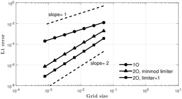
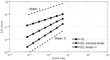
Figure 2: (a) $L_{1}$ error norm vs grid size, (b) $L_{2}$ error norm vs grid size

The $L_{1}$ and $L_{2}$ errors of the present scheme for I order accuracy are tabulated in Table 1. The II order results are tabulated in Table 2 (with limiter) and Table 3 (without limiter, i.e., $\phi$= 1) respectively. The log-log plots comparing the EOC with slopes 1 and 2 are shown in Figure 2.

6.2 1D Euler tests

$x_{1}$	$x_{2}$	$x_{0}$	$\rho_{L}$	$u_{L}$	$p_{L}$	$\rho_{R}$	$u_{R}$	$p_{R}$	$t_{final}$
0	1	0.5	1.0	1.0	$\frac{1}{\gamma M(=2)^{2}}$	$\frac{\frac{\gamma+1}{\gamma-1}\frac{p_{R}}{p_{l}}+1}{\frac{\gamma+1}{\gamma-1}+\frac{p_{R}}{p_{L}}}$	$\sqrt{\frac{\gamma(2+(\gamma-1)M^{2})p_{R}}{(2\gamma M^{2}+1-\gamma)\rho_{R}}}$	$p_{L}\frac{2\gamma M^{2}-(\gamma-1)}{\gamma+1}$	1.5
0	1	0.5	1.4	0	1.0	1.0	0.0	1.0	2.0
0	1	0.5	3.86	-0.81	10.33	1.0	-3.44	1.0	1.0
0	1	0.5	1.4	0.1	1.0	1.0	0.1	1.0	1.0
0	1	0.5	1.0	0.0	1.0	0.125	0.0	0.1	0.25
0	1	0.5	1.0	-2.0	0.4	1.0	2.0	0.4	0.15
0	1	0.5	1.0	0.0	1000.0	1.0	0.0	0.01	0.012
0	1	0.4	5.99924	19.5975	460.894	5.99242	-6.19633	46.0950	0.035
0	1	0.8	1.0	-19.59745	1000.0	1.0	-19.59745	0.01	0.012
-1	1	-0.8	3.857143	2.629369	10.3333	1+ 0.2$sin(5\pi x)$	0.0	1.0	0.47

Table 4: Initial condition for 1D test cases

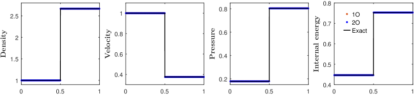
Figure 3: Test case 1: Steady shock

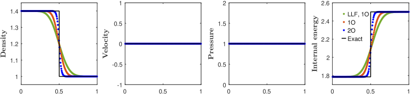
Figure 4: Test case 2: Steady contact-discontinuity

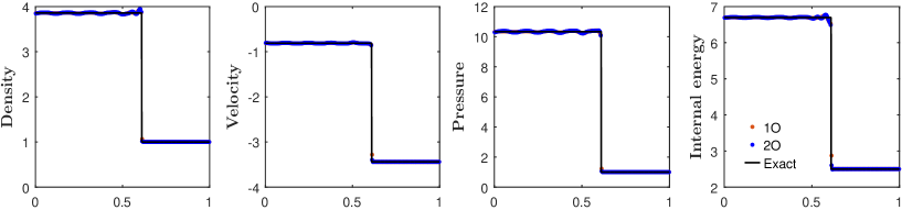
Figure 5: Test case 3: Slowly moving shock

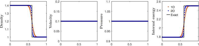
Figure 6: Test case 4: Slowly moving contact-discontinuity

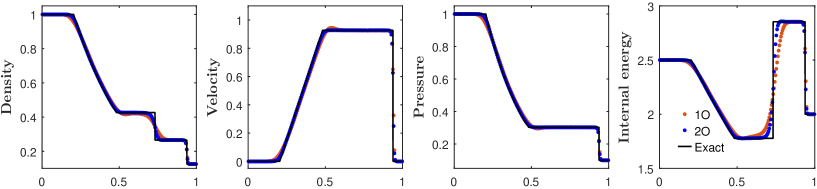
Figure 7: Test case 5: Sod’s shock tube problem, t=0.25

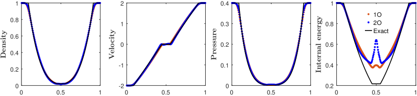
Figure 8: Test case 6: Overheating problem

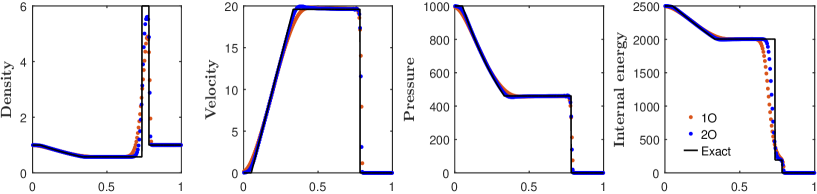
Figure 9: Test case 7: Left half portion of Woodward and Colella problem

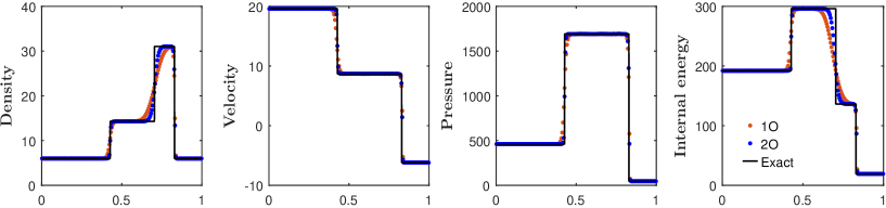
Figure 10: Test case 8: Colliding strong shocks

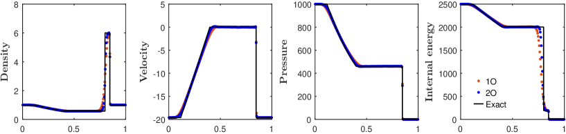
Figure 11: Test case 9

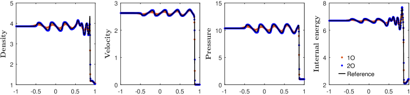
Figure 12: Test case 10: Shock-entropy wave collision

We have solved an extensive set of benchmark 1D Euler problems to test the accuracy and robustness of our numerical scheme. The initial conditions for these test cases have been tabulated in Table 4. In the table, $x_{1}$ and $x_{2}$ denote the two ends of the domain, whereas $x_{0}$ is the position of initial discontinuity. For all the test cases, the cell size $\Delta x$= 0.005, CFL number $\sigma$= 0.8, and Neumann boundary conditions (at the two ends) are applied. Test case 1 has a steady shock, introduced as an initial discontinuity, with a freestream Mach 2 flow. The results in Figure 3 show that our numerical scheme captures the steady shock exactly for both first and second order accuracy. Test case 2 comprises of a steady contact discontinuity as the initial condition. The results in Figure 4 show that our numerical scheme captures the discontinuity sharply and with much less numerical diffusion than the Local Lax-Friedrichs (LLF) scheme. Test case 3 comprises of a slowly moving shockwave. The results in Figure 5 show the shock captured over few cells, with minor oscillations. The slowly moving contact-discontinuity in Test case 4 (Figure 6 ) is also captured with reasonable accuracy, without any oscillations. Test cases 5 to 9 are taken from Toro ([28]). Test case 5 is the Sod’s shock tube problem. Its solution consists of a shock wave and a contact-discontinuity traveling to the right and an expansion wave (containing a sonic point) going to the left. The results in Figure 7 show that no entropy violating expansion shock is formed. Test case 6 is the well-known overheating problem for which several Riemann solvers fail. Its solution consists of two strong symmetric expansions to the left and right, with a contact discontinuity of vanishing strength in the middle. For this test case, pressure at center reaches near vacuum, making it a suitable test case for assessing the performance of a scheme at low densities. The results in Figure 8 show that our scheme does not fail for this test case, and captures the the expansions accurately. However, there is an increase in internal energy at the center, which is observed for many numerical methods due to numerical overheating. Test case 7 to 9 test the robustness of a scheme in handling large gradients. Test case 7 is the left half of the blast wave problem of Woodward and Colella. Its solution comprises of a strong shock to the right, a contact discontinuity in middle and an expansion fan to the left. Test case 8 involves collision of two strong shocks; its solution consists of a left facing shock (traveling very slowly to the right), a right traveling contact discontinuity and a right traveling shock. Test case 9 consists of a left rarefaction wave, a right traveling shock wave and a stationary contact discontinuity. The results for these test cases are shown in Figures 9 to 11. The results are reasonably accurate. Test case 10 is the shock-entropy wave interaction problem. It comprises of a Mach 3 shock traveling right and interacting with stationary medium with an initial sinusoidal perturbation in density. This initial disturbance gives rise to continuous interaction of smooth flow with discontinuities. Similar interactions occur in compressible turbulence simulations. This makes it a suitable problem to test the ability of a numerical scheme to resolve complex interactions, which can be used in turbulent computations. The results in Figure 12 show that our second order accurate solution matches well with the reference (fine grid) solution.

6.3 2D Euler tests

Some standard 2D inviscid test cases are solved to showcase the accuracy, robustness as well as positivity preserving properties of our proposed numerical method. The boundary conditions used have been derived for our kinetic model in C. For all the test cases, CFl no $\sigma$= 0.8, unless mentioned otherwise. For steady state results, our strategy is to evolve the solution in time until a minimum density residual of $10^{-10}$ or maximum time steps of 50000 is reached, whichever occurs earlier.

6.3.1 Oblique shock reflection

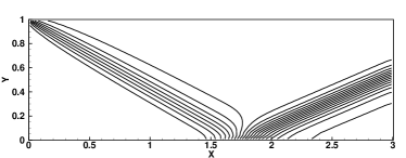
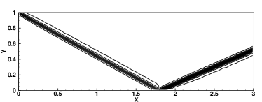
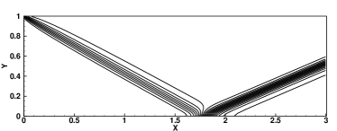
Figure 13: Oblique shock reflection with shock angle $29^{\circ}$, inflow Mach no. 2.9 - Pressure contours (0.7:0.1:2.9), Top) I order and II order accurate results for $120\times 40$ grid, Bottom) I order and II order accurate results on $240\times 80$ grid

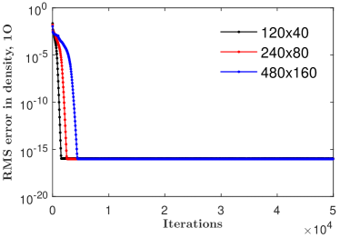
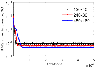
Figure 14: Oblique shock reflection test case: RMS error in density vs number of iterations for a) I order result, b) II order result

This test case comprises of an oblique shock striking a solid wall at an incident shock angle of $29^{\circ}$ and reflecting from it [29]. The freestream flow from left to right has a Mach no. of 2.9. The computational domain is $[0,3]\times[0,1]$. Left boundary has supersonic inflow, hence freestream conditions are applied there. Post-shock conditions using compressible flow relations are applied at the top. Flow tangency (inviscid wall) conditions are applied at the bottom and supersonic outflow conditions are applied at the right boundary. Freestream initial conditions are used. The pressure contours for our first and second order accurate steady state results are shown in Figure 13. The shock profile is sharper for a finer grid and for higher order accuracy. Figure 14 shows the variation in root-mean-square (RMS) error in density with number of time iterations for different cell sizes. The results are shown for both first and second order accuracy.

6.3.2 Supersonic flow over a compression ramp

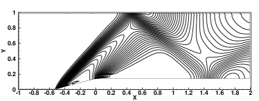
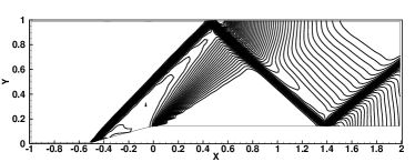
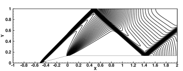
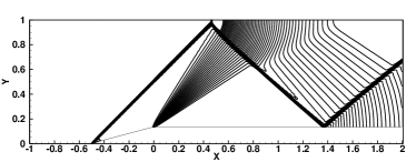
Figure 15: Mach 2 flow over a $15^{\circ}$ ramp - Pressure contours (1.1:0.05:3.8), Top) I order and II order accurate results on $120\times 40$ grid, Bottom) I order and II order accurate results on $480\times 160$ grid

This test case comprises of a Mach 2 flow over a $15^{\circ}$ compression ramp in a wind tunnel [30]. The computational domain is $[1,2]\times[0,1]$ with a $15^{\circ}$ ramp at the bottom from x= -0.5 to x= 0. The applied boundary conditions are: supersonic inflow at the left boundary, flow tangency conditions at the top and bottom walls, and supersonic outflow conditions at the right boundary. Freestream initial conditions are used. The steady state results are shown in Figure 15. The solution comprises of an oblique shock originating at the concave corner and expansion fans starting from the convex corner. The oblique shock strikes and reflects from the top and bottom walls while also interacting with the expansion fan. As our contours show, no entropy-violating expansion shocks are formed.

6.3.3 Grid-aligned oblique shock on a non-Cartesian grid

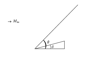
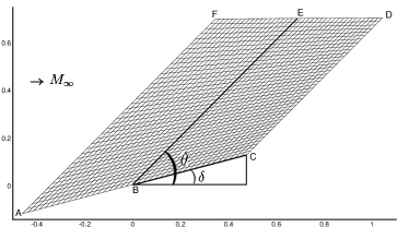
Figure 16: Mach 2 flow over a $15^{\circ}$ wedge, a) Setup showing the wedge and the oblique shock , b) Computational domain and mesh

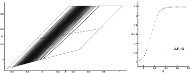
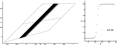
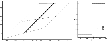
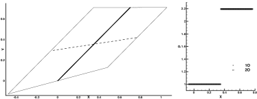
Figure 17: Pressure contours (1.1:0.0333:2.2) and pressure variation along the dashed ($j$= Ny/2) line for I order and II order accuracy: Top) LLF scheme on a $40\times 40$ grid, Bottom) Present scheme on $40\times 40$ and $160\times 160$ grids.

This test case has been devised to test the ability of a numerical scheme to capture a grid-aligned steady shock on a non-Cartesian grid. The flow conditions have been taken from the previous test case, with a freestream Mach 2 flow from left to right across a flat surface inclined at a wedge angle $\delta=15^{\circ}$ with the flow. For $\gamma$= 1.4 (assumed throughout this work) and $\delta=15^{\circ}$, the oblique shock relations give us a shock wave angle of $\theta=45.3436^{\circ}$. The computational domain ABCDEF along with the mesh is shown in Figure 16. The boundary AC is aligned at wedge angle $\delta$ to the incoming freestream flow, with the wall starting at B ((0,0)) and ending at C. The boundaries AF and CD, as well as all lines in between, are aligned at shock wave angle $\theta$ to the incoming flow. Finally, FED is parallel to the freestream flow. The domain is initialized with freestream conditions. Supersonic inflow conditions are applied at AF, and supersonic outflow conditions are applied at the boundaries AB and CD. Flow tangency (inviscid wall) conditions are applied at BC. Through numerical experiments, we have observed that a constant extrapolation at the boundary FED is effective in preventing any deformation of the shock near the top. Thus, we have applied constant extrapolation at the boundary FD. The steady state results for this problem are shown in Figure 17. We observe that the more diffusive Local Lax-Friedrichs (LLF) scheme diffuses the shock over many cells. Our scheme, on the other hand, captures the grid-aligned oblique shock exactly for first as well as second order accuracy.

6.3.4 Hypersonic flow over a half-cylinder

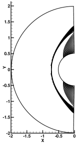
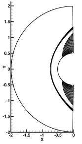
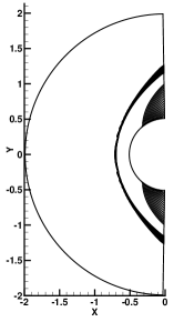
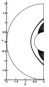
Figure 18: Hypersonic flow past a half-cylinder, density contours (2:0.2:5) on $100\times 80$ grid (a) Mach 6 flow, I order (b) Mach 6 flow, II order, (c) Mach 20 flow, I order (d) Mach 20 flow, II order

This test case assesses a scheme for a form of numerical shock instability called carbuncle phenomenon. For this problem, we consider Mach 6 and Mach 20 flows over a half-cylinder. The computational domain taken is $(r,\theta)\in[0.5,2]\times[\frac{\pi}{2},\frac{3\pi}{2}]$, with constant grid spacing along $r$ and $\theta$ directions. Supersonic inflow conditions are applied at $r=2$ and flow tangency conditions are applied at $r=0.5$. Supersonic outflow conditions are applied at $\theta=\frac{\pi}{2}$ and $\theta=\frac{3\pi}{2}$ boundaries. Freestream initial conditions are used. For this test case, the steady state solution consists of a bow shock formed in front of and detached from the half-cylinder. Many numerical schemes, especially the Riemann solvers like the Roe scheme, develop an unusual feature called as carbuncle shock, with bow shock breaking on the stagnation line [20]. These carbuncle shocks are often considered as spurious numerical artifacts and a significant research effort is spent on obtaining carbuncle-free solutions. Our results are shown in Figure 18 and no carbuncle shock is observed in our solution.

6.3.5 Supersonic flow over a forward facing step

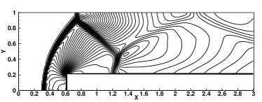
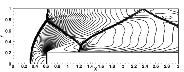
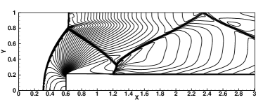
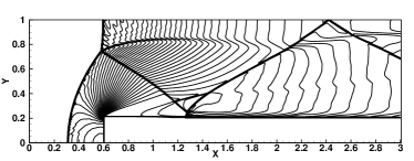
Figure 19: Mach 3 flow over a forward-facing step in wind tunnel, $t=4$, density contours (1:0.15:6.5); Top) I order and II order accurate results on $240\times 80$ grid, Bottom) I order and II order accurate results on $960\times 320$ grid

For this unsteady problem, we consider a Mach 3 flow over a forward facing step in a wind tunnel [31]. The dimensions of the wind tunnel are $[0,3]\times[0,1]$. The step is 0.2 unit high and located at the bottom at a distance of 0.6 units from the left end. The boundary conditions applied are: supersonic inflow at the left boundary, flow tangency conditions at the top and bottom walls (including the step), and supersonic outflow conditions at the right boundary. Freestream initial conditions are used. A lambda shock formed near the top boundary is visible at time $t=4$. A slip stream can be seen beyond the triple point, which can be captured well only by low diffusive schemes. The first and second order results for this test case are shown in Figure 19.

6.3.6 Odd-even decoupling

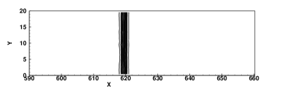
Figure 20: Mach 6 shock wave through a rectangular duct at $t=100$, $800\times 20$ grid, density contours; (a) I order and (b) II order

This test case consists of a planar Mach 6 shock propagating through stationary medium in a rectangular duct [20]. A Cartesian mesh of $800\times 20$ square cells is used. The grid is perturbed along the center-line as follows

$$(y_{i,j})_{mid}=\left\{\begin{array}[]{c}(y_{i,j})_{mid}+10^{-3},\ \text{if}\ i\ \text{is even}\\ (y_{i,j})_{mid}-10^{-3},\ \text{if}\ i\ \text{is odd}\end{array}\right\}$$ (127)

The right traveling shock is located at the interface between $20^{th}$ and $21^{st}$ cell at initial time. The solution is sought at time $t=100$. For this problem, low diffusive schemes like the Roe scheme develop oscillations due to a type of numerical instability called odd-even decoupling, which then destroys the solution. As our results in Figure 20 show, our scheme is free from this form of instability.

6.3.7 Double Mach reflection

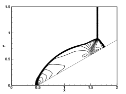
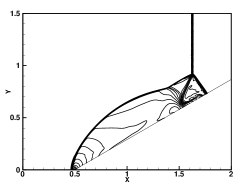
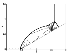
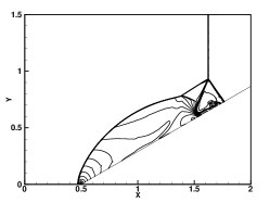
Figure 21: Double Mach reflection for Mach 5.5 shock across a $30^{\circ}$ wedge, $t=0.25$, density contours (1.5:0.5:19); Top) I order and II order accurate results on $400\times 400$ grid, Bottom) I order and II order accurate results on $1200\times 1200$ grid

In this test case, a planar Mach 5.5 shock travels across a $30^{\circ}$ wedge [20]. The computational domain taken is $[0,2]\times[0,1.5]$ with a $30^{\circ}$ wedge at the bottom starting at $x=0.5$. At initial time, the right- traveling shock is placed at x= 0.25, with stationary medium to its right. Moving shock relations are used to determine the initial flow state to the left. Following boundary conditions are applied: initial left flow state at the left boundary, flow tangency conditions at the top and bottom boundaries, and constant extrapolation at the right boundary. When the moving shock collides with the wedge, it reflects over the surface as Mach reflection. The wave configuration consists of the initial shock, the reflected shock, one Mach stem and one slip stream, all of which meet at a single triple point. Figure 21 shows the numerical solution of this unsteady problem at $t=0.25$. Some low diffusion schemes produce an unphysical kinked Mach stem. No such kinked Mach stem is seen in our results.

6.3.8 Shock diffraction

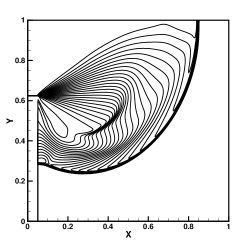
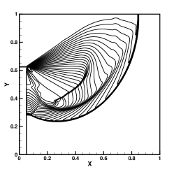
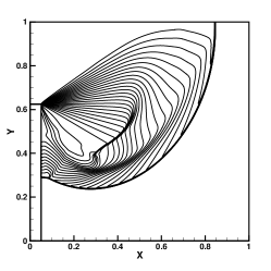
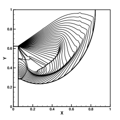
Figure 22: Shock diffracting around a $90^{\circ}$ corner, $t=0.1561$, density contours (0.5:0.25:6.75); Top) I order and II order accurate results on $400\times 400$ grid, Bottom) I order and II order accurate results on $1200\times 1200$ grid

In this test case, a planar Mach 5.09 shock diffracts around a $90^{\circ}$ corner [20]. The computational domain taken is $[0,1]\times[0,1]$, with a corner at the bottom left end of width 0.05 unit and height 0.625 unit respectively. At initial time, the planar shock is located at x= 0.05, traveling right into stationary medium. The boundary conditions are: initial left flow state at the left boundary, flow tangency conditions at the top and for the corner, and constant extrapolation at the right and bottom boundaries. Figure 22 shows our numerical solution for this unsteady problem at time t= 0.1561. The solution has a complex wave structure comprising of the incident planar shock, the diffracted shock, a strong expansion fan and a slip stream. Without an entropy fix, several low-diffusive schemes give rise to unphysical expansion shocks. Some Riemann solvers also produce oscillations near the location where the shock hits the top boundary. Our results are free of expansion shocks and oscillations. All flow features are captured well.

6.3.9 Positivity test cases

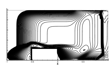
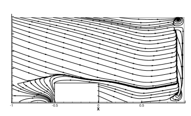
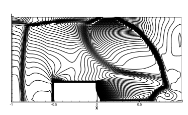
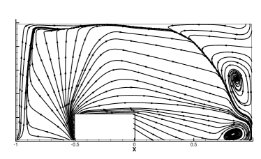
Figure 23: Parent Test case 8 (2D enclosure), I order results; Top) Pressure contours and streamlines at t= 0.00047, Bottom) Pressure contours and streamlines at t= 0.000955

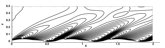
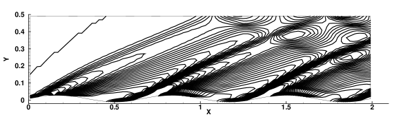
Figure 24: Parent Test case 11 (2D channel with wavy wall); pressure contours; (a) I order and (b) II order

In this section, we have solved test cases taken from Parent [22] which test a numerical scheme for its positivity preservation property. These test cases have large initial Mach numbers which create strong expansions (and thus low pressures) within the first few iterations, making them difficult to solve numerically. Since our proposed scheme for first order accuracy is positivity preserving, it is expected not to fail for these test cases and the results confirm this expectation. The first test case that we have solved is the 2D inclosure problem (Parent test case 8). It comprises of a rectangular domain of dimensions $[-1,1]\times[0,1]$ with a cut-out at the bottom from x=-0.52 to x=0, and having a height of 0.24 units. A rectangular grid with fixed cell size of 0.02 units along both dimensions is chosen. CFL no. taken is 0.25. Since the flow is enclosed, flow tangency conditions are applied at all boundaries. The initial conditions are as follows.

Left state, x$$\leq \ T=35\ K,\ M_{x}=10,\ M_{y}=-3,\ p=0.1\ bar$$ 0:

Right state, x$$> \ T=35\ K,\ M_{x}=10,\ M_{y}=2,\ p=0.1\ bar$$ 0: (128)

This initial flow strikes and reflects from the walls and the cut-out, creating complex flow features having strong pressure gradients. Our first order accurate results in Figure 23 show the pressure contours and streamlines at times t= 0.00047 and t= 0.000955. Our first order scheme thus successfully captures these strong gradients. Our second order method fails for this test case; it is not unexpected since our second order scheme is not necessarily positivity preserving. The next test case that we have solved comprises of Mach 3 flow in a 2D channel with wavy wall. (Parent test case 11). The computational domain is $[0,2]\times[0,0.5]$, with wavy wall at the bottom, given by y= $\frac{1}{50}sin(3\pi x)$. The grid is composed of 100 $\times$ 25 uniformly spaced cells. At initial time, flow throughout the domain is initialized with the following conditions:

$$T=300\ K,\ M_{x}=3,\ M_{y}=0,\ p=0.102\ bar$$ (129)

Supersonic inflow and outflow conditions are applied at the left and right boundaries respectively, whereas flow tangency conditions are applied at the top and bottom. The wavy wall at the bottom alternately compresses and expands the supersonic flow. As a result, we get alternating oblique shocks and expansion fans emanating from the wavy wall. Our first and second order accurate steady state results (Figure 24) capture these flow features accurately.

6.3.10 NACA0012 airfoil test cases

We have solved some benchmark test cases for the symmetric NACA0012 airfoil [32, 33]. For these tests, an O-type structured grid with dimensions of 25 times the chord length is used around the airfoil. Farfield conditions described in C are applied at the outer boundary, whereas flow tangency conditions are applied at the airfoil surface. Periodic conditions are applied along $\eta$-direction where the first and last grid meet. Freestream initial conditions are used, and steady state solution is sought. Numerical tests are done for the following supersonic, transonic and subsonic test cases.

1. $M_{\infty}=$ 1.2, A.O.A. (Angle of attack) = $0^{\circ}$

2. $M_{\infty}=$ 1.2, A.O.A. = $7^{\circ}$

3. $M_{\infty}=$ 0.8, A.O.A. = $1.25^{\circ}$

4. $M_{\infty}=$ 0.85, A.O.A. = $1^{\circ}$

5. $M_{\infty}=$ 0.63, A.O.A. = $2^{\circ}$

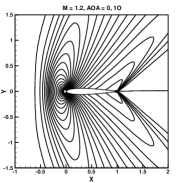
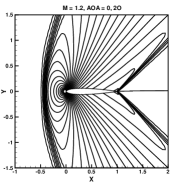
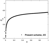
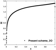
Figure 25: NACA0012, $M_{\infty}=$ 1.2, A.O.A$=0^{\circ}$, $438\times 107$ grid: a) I order, b) II order, pressure contours (0.4:0.05:2.0), c) $C_{p}$ vs $x$, d) $M$ vs $x$ along the top and bottom surfaces of the airfoil.

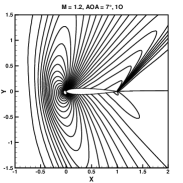
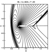
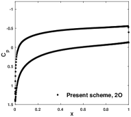
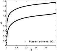
Figure 26: NACA0012, $M_{\infty}=$ 1.2, A.O.A$=7^{\circ}$, $438\times 107$ grid: a) I order, b) II order, pressure contours (0.4:0.05:2.0), c) $C_{p}$ vs $x$, d) $M$ vs $x$ along the top and bottom surfaces of the airfoil.

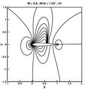
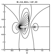
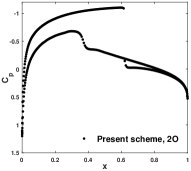
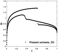
Figure 27: NACA0012, $M_{\infty}=$ 0.8, A.O.A$=1.25^{\circ}$, $438\times 107$ grid: a) I order, b) II order, pressure contours (0.4:0.05:2.0), c) $C_{p}$ vs $x$, d) $M$ vs $x$ along the top and bottom surfaces of the airfoil.

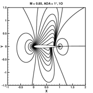
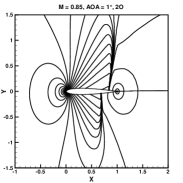
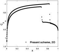
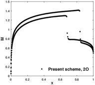
Figure 28: NACA0012, $M_{\infty}=$ 0.85, A.O.A$=1^{\circ}$, $438\times 107$ grid: a) I order, b) II order, pressure contours (0.4:0.05:2.0), c) $C_{p}$ vs $x$, d) $M$ vs $x$ along the top and bottom surfaces of the airfoil.

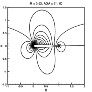
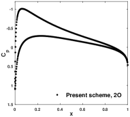
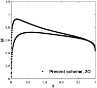
Figure 29: NACA0012, $M_{\infty}=$ 0.63, A.O.A$=2^{\circ}$, $438\times 107$ grid: a) I order, b) II order, pressure contours (0.7:0.02:1.4), c) $C_{p}$ vs $x$, d) $M$ vs $x$ along the top and bottom surfaces of the airfoil.

For the above test cases, the pressure contours for first and second order accuracy, as well as the variation of pressure coefficient $C_{p}$(=$\frac{p-p_{\infty}}{0.5\rho_{\infty}|\textbf{u}|^{2}_{\infty}}$) and Mach no. $M$(= $\frac{|\textbf{u}|}{a}$) along the top and bottom surfaces of the airfoil are plotted in Figures (25) to (29). The results demonstrate the accuracy of our numerical scheme (e.g. near exact capture of a shock in the third airfoil test case (Figure 27)) and its ability to resolve supersonic as well as high-subsonic flows.

6.4 2D Viscous tests

Some viscous test cases are solved to demonstrate the ability of our numerical scheme to solve viscous equations and resolve viscous flow features like boundary layers. For these problems, the gradient terms in the viscous fluxes are computed using auxiliary volume method.

6.4.1 Sod’s shock tube problem

This test is the two-dimensional version of the Sod’s shock tube problem. The computational domain taken is $[0,1]\times[0,0.3]$. The initial conditions for this unsteady problem are given below.

Left state, x$$\leq \rho_{L}=1,\ (u_{1})_{L}=0,\ (u_{2})_{L}=0,\ p_{L}=1$$ 0.5:

Right state, x$$> \rho_{R}=0.125,\ (u_{1})_{R}=0,\ (u_{2})_{R}=0,\ p_{R}=0.1$$ 0.5: (130)

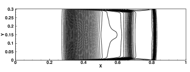
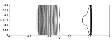
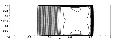
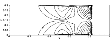
Figure 30: Sod’s shock tube problem (140x 140): Top) Density and pressure contours, Bottom) $u_{1}$ and $u_{2}$ velocity contours.

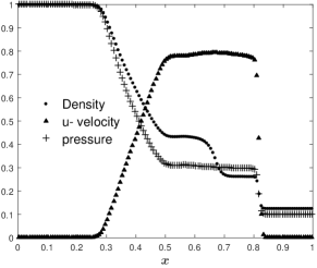
Figure 31: Sod’s shock tube problem (140x 140), flow variables along the center-line

The prescribed initial Reynolds no., Re= 25000, and Prandtl no., Pr= 0.72, are used. No-slip conditions (viscous wall) are applied at the top and bottom boundaries, and Neumann conditions are applied at the left and right boundaries. The domain is discretized into $140\times 140$ cells, with constant cell size along x-direction. Along y-direction, the cells are geometrically stretched from the walls to the center with a regular increment of $4\%$. The initial discontinuity leads to flow from left to right, with a shock wave and a contact discontinuity traveling right, and rarefaction waves going left. Flow behind the shock leads to the formation of boundary layers at the top and bottom, which bring in non-uniformity of flow along the transverse direction. Figure 30 shows the contours of pressure, density, $u_{1}$ and $u_{2}$ for the second order accurate results at time t= 0.2136. Flow properties at the center-line have been plotted against the length of the shock tube in Figure 31. Flow features like the shock, the contact discontinuity and expansion are captured well. The $u_{2}$ contours show that the boundary layers at the walls behind the shock are also resolved by our scheme.

6.4.2 Shock-boundary layer interaction

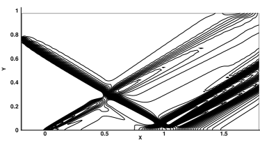
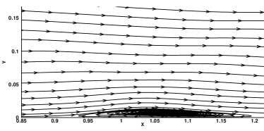
Figure 32: Test case: Shock wave- boundary layer interaction (140x 120), a) 2O Pressure contours, b) Streamlines showing the recirculation zone

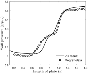
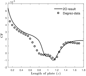
Figure 33: Test case: Shock wave-boundary layer interaction (140x 120), a) Wall pressure, b) Skin friction coefficient along the length of the plate

This viscous problem comprises of an oblique shock, formed by a supersonic freestream flow with Mach no. $M_{\infty}$= 2.15 and shock angle of $30.8^{\circ}$, striking a flat plate at the bottom on which a laminar boundary layer is evolving [34]. This causes the flow to locally separate and then reattach to the surface. The reflected waves consist of compression waves converging into a shock, then expansion waves, which are followed again by compression waves. The freestream Reynolds no., $Re=10^{5}$, and Prandtl no., Pr= 0.72, are prescribed. The computational domain taken is $[-0.2,1.8]\times[0,1]$. Supersonic inflow conditions are applied at the left boundary for y$\leq$ 0.765. Whereas post-shock conditions are applied for y$>$0.765 at the left boundary, as well as for the entire top boundary. At the bottom, we use flow symmetry conditions for x $\leq 0.2$, and viscous wall conditions for x $>$0.2. Supersonic outflow conditions are applied at the right boundary. We have discretized the domain into $140\times 120$ cells, with constant grid spacing along x direction and a geometrically stretched grid with a regular $4.5\%$ increment in grid spacing along y direction. Additionally, for this test, the limiter functions in the inviscid fluxes are set to 1. Figure 32 shows the pressure contours and streamlines of our second order accurate steady state results. Our results show that the reflected compression and expansion waves as well as the recirculated flow in the separated flow region are properly captured. The wall pressure $\frac{p_{w}}{p_{\infty}}$ and skin friction coefficient $c_{f}$ along the length of the plate are plotted in Figure 33. Our results match reasonably well with the data from Degrez et al. [34].

6.4.3 Supersonic flow over a bump

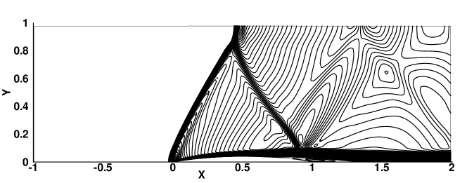
Figure 34: Test case: Supersonic flow over a bump (240x 80), 2nd order, Mach contours

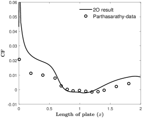
Figure 35: Test case: Supersonic flow over a bump (240x 80), Skin friction coefficient along wall

In this test case, we consider a Mach 1.4 flow over a circular bump in a channel [35]. The computational domain taken is $[-1,2]\times[0,1]$ with a $4\%$ circular arc at the bottom from x= 0 to x= 1. The freestream Reynolds no., Re= 8000, and Prandtl no., Pr= 0.72, are prescribed. Supersonic inflow conditions are applied at the left boundary and supersonic outflow conditions are applied at the right boundary. At the bottom, flow symmetry conditions are imposed for x $\leq$0, whereas no-slip (viscous wall) conditions are applied for x$>$0. Flow tangency conditions are applied at the top wall. The domain is discretized into $240\times 80$ cells, with constant grid spacing along x direction and a geometrically stretched grid with a regular $4.5\%$ increment in grid spacing along y direction. The interface inviscid fluxes have limiters set to 1 for this test as well. The Mach contours for the second order accurate steady state result (Figure 34) show an oblique shock forming at the leading edge of the bump. This shock reflects from the top wall, and then interacts with the separated flow at the end of the bump and reflects from it. In Figure 35, the skin friction coefficient is plotted along the length of the bottom wall and compared with the data from Parthasarathy & Kallenderis [35].

7 Conclusions

We have formulated a new kinetic model for the Euler equations which comprises of two flexible velocities in 1D which satisfy positivity preservation conditions. Our asymmetrical model (in terms of normal velocity at the interface) captures a steady shock exactly without needing any shock sensor. Our more diffusive symmetrical model generates solutions that are entropic. We have used our own version of kinetic relative entropy and an additional criterion to identify smoothly varying flow regions, where we switch from the asymmetrical model to the symmetrical model. We have also obtained a limit on the time step, which ensures positivity preservation as well as numerical stability for the resulting numerical scheme. We have extended our basic scheme to second order accuracy using a flux limited approach and a higher order Runge-Kutta method. However, positivity preservation has not been ensured for our second order scheme, and that remains an open problem. In 2D, we have formulated a novel three velocity kinetic model, with the velocities aligned to the cell-interface such that the resulting normal flux is locally one-dimensional and the grid-aligned steady shocks are captured exactly. We have also obtained inviscid normal boundary fluxes in flux difference split form at certain boundaries for our kinetic model. Finally, we have used our inviscid scheme along with the viscous fluxes to numerically solve the viscous equations. We have solved benchmark 1D and 2D compressible flow test cases to showcase the robustness and accuracy of our numerical scheme.

CRediT author statement

Shashi Shekhar Roy: Conceptualization, Methodology, Investigation, Software, Validation, Formal analysis, Writing- Original draft.

S. V. Raghurama Rao: Investigation, Supervision, Resources, Writing- Review & Editing.

Declaration of competing interest

The authors declare that they have no known financial interests or personal relationships with any other people or organizations that could influence the work presented here.

Data availability

No data was used for research described in this article.

Appendix A Positivity condition

We consider the requirement of positivity of the term $\left(\lambda_{p}\right)_{j+\frac{1}{2}}\textbf{U}_{j+1}-\textbf{G}_{j+1}$. That is,

$$\left(\lambda_{p}\right)_{j+\frac{1}{2}}\textbf{U}_{j+1}-\textbf{G}_{j+1}=\begin{bmatrix}G_{1}&G_{2}&G_{3}\end{bmatrix}^{T}\in\textbf{W}$$ (131)

Since $\lambda_{p}\geq$0, the condition (131) can be restated as

$$\textbf{U}_{j+1}-\textbf{G}_{j+1}/\left(\lambda_{p}\right)_{j+\frac{1}{2}}=\begin{bmatrix}U_{1}&U_{2}&U_{3}\end{bmatrix}^{T}\in\textbf{W}$$ (132)

Now, the requirement of non-negative density and pressure in (132) implies that,

$$U_{1}\geq 0\text{ and }2U_{1}U_{3}-U^{2}_{2}\geq 0\ \left(\text{equivalently, }G_{1}\geq 0\text{ and }2G_{1}G_{3}-G^{2}_{2}\geq 0\right)$$ (133)

The condition $G_{1}\geq 0$ gives us

$$\rho_{j+1}\left(\lambda_{p}\right)_{j+\frac{1}{2}}-(\rho u)_{j+1}\geq 0\Rightarrow\left(\lambda_{p}\right)_{j+\frac{1}{2}}\geq u_{j+1}$$ (134)

Similarly, the condition $2G_{1}G_{3}-G^{2}_{2}\geq 0$ leads to

$$\begin{split}&2\left[\rho_{j+1}\left(\lambda_{p}\right)_{j+\frac{1}{2}}-(\rho u)_{j+1}\right]\left[(\rho E)_{j+1}\left(\lambda_{p}\right)_{j+\frac{1}{2}}-\left\{\left(\rho E+p\right)u\right\}_{j+1}\right]-\left[(\rho u)_{j+1}\left(\lambda_{p}\right)_{j+\frac{1}{2}}-(\rho u^{2}+p)_{j+1}\right]^{2}\geq 0\\ &\Rightarrow p_{j+1}\left[\frac{2}{\gamma-1}\rho_{j+1}\left\{\left(\lambda_{p}\right)_{j+\frac{1}{2}}-u_{j+1}\right\}^{2}-p_{j+1}\right]\geq 0\text{ (on simplifying)}\\ &\Rightarrow\left(\lambda_{p}\right)_{j+\frac{1}{2}}\geq u_{j+1}+\sqrt{\frac{\gamma-1}{2\gamma}}a_{j+1}\end{split}$$ (135)

We note that the condition (135) automatically satisfies (134). Thus, the positivity condition (131) leads to a limitation on $\lambda_{p}$ as specified in (135).

Appendix B Linear Stability Analysis

A von Neumann linear stability analysis of the advective part of the 1D Boltzmann equations is done for first order accuracy. We consider the scalar linear advection equation as the macroscopic governing equation, for simplicity. The advective part of the 1D Boltzmann equation can then be written as

$$\frac{\partial}{\partial t}\begin{bmatrix}f_{1}\\ f_{2}\end{bmatrix}+\frac{\partial}{\partial x}\left\{\begin{bmatrix}\lambda_{p}&0\\ 0&\lambda_{m}\end{bmatrix}\begin{bmatrix}f_{1}\\ f_{2}\end{bmatrix}\right\}=0$$ (136)

We discretize (136) for first order accuracy, while noting that for modeling the macroscopic linear advection equation , $\lambda_{p}$ and $\lambda_{m}$ are taken as constants.

$$\frac{1}{\Delta t}\left\{\begin{bmatrix}(f_{1})^{n+1}_{j}\\ (f_{2})^{n+1}_{j}\end{bmatrix}-\begin{bmatrix}(f_{1})^{n}_{j}\\ (f_{2})^{n}_{j}\end{bmatrix}\right\}+\frac{1}{\Delta x} \left\{\begin{bmatrix}\frac{1}{2}\left(\lambda_{p}(f_{1})^{n}_{j}+\lambda_{p}(f_{1})^{n}_{j+1}\right)-\frac{\lambda_{p}}{2}\left((f_{1})^{n}_{j+1}-(f_{1})^{n}_{j}\right)\\ \frac{1}{2}\left(\lambda_{m}(f_{2})^{n}_{j}+\lambda_{m}(f_{2})^{n}_{j+1}\right)+\frac{\lambda_{m}}{2}\left((f_{2})^{n}_{j+1}-(f_{2})^{n}_{j}\right)\end{bmatrix}-\right.$$ (137)

$$\left.\begin{bmatrix}\frac{1}{2}\left(\lambda_{p}(f_{1})^{n}_{j-1}+\lambda_{p}(f_{1})^{n}_{j}\right)-\frac{\lambda_{p}}{2}\left((f_{1})^{n}_{j}-(f_{1})^{n}_{j-1}\right)\\ \frac{1}{2}\left(\lambda_{m}(f_{2})^{n}_{j-1}+\lambda_{m}(f_{2})^{n}_{j}\right)+\frac{\lambda_{m}}{2}\left((f_{2})^{n}_{j}-(f_{2})^{n}_{j-1}\right)\end{bmatrix}\right\}=0$$

or,

$$\frac{1}{\Delta t}\left\{\begin{bmatrix}(f_{1})^{n+1}_{j}\\ (f_{2})^{n+1}_{j}\end{bmatrix}-\begin{bmatrix}(f_{1})^{n}_{j}\\ (f_{2})^{n}_{j}\end{bmatrix}\right\}+\frac{1}{\Delta x}\left\{\begin{bmatrix}\lambda_{p}(f_{1})^{n}_{j}\\ \lambda_{m}(f_{2})^{n}_{j+1}\end{bmatrix}-\begin{bmatrix}\lambda_{p}(f_{1})^{n}_{j-1}\\ \lambda_{m}(f_{2})^{n}_{j}\end{bmatrix}\right\}=0$$ (138)

Thus, for the linear case, the flux difference formulation is equivalent to an upwind method with Courant-type splitting. Next, we introduce Fourier expansions for $f_{1}$ and $f_{2}$ as follows.

$$(f_{1})^{n}_{j} = (\widetilde{f}_{1})^{n}e^{Ij\theta}$$

$$(f_{2})^{n}_{j} = (\widetilde{f}_{2})^{n}e^{Ij\theta}$$ (139)

where I=$\sqrt{-1}$. Substituting (139) in (138) and simplifying, we get

$$\begin{bmatrix}(\widetilde{f}_{1})^{n+1}\\ (\widetilde{f}_{2})^{n+1}\end{bmatrix}=\begin{bmatrix}\left\{1+\frac{\lambda_{p}\Delta t}{\Delta x}(e^{-I\theta}-1)\right\}&0\\ 0&\left\{1-\frac{\lambda_{m}\Delta t}{\Delta x}(e^{I\theta}-1)\right\}\end{bmatrix}\begin{bmatrix}(\widetilde{f}_{1})^{n}\\ (\widetilde{f}_{2})^{n}\end{bmatrix}$$ (140)

or

$$\begin{bmatrix}\widetilde{f}_{1}\\ \widetilde{f}_{2}\end{bmatrix}^{n+1}=\textbf{A}\begin{bmatrix}\widetilde{f}_{1}\\ \widetilde{f}_{2}\end{bmatrix}^{n}$$ (141)

Now, for the above scheme to be stable, i.e., for the amplification factor to be less than or equal to 1, the absolute value of the eigenvalues of A should be less than or equal to 1. Therefore,

$$|1+\frac{\lambda_{p}\Delta t}{\Delta x}(e^{-I\theta}-1)|\leq 1,\text{ and }|1-\frac{\lambda_{m}\Delta t}{\Delta x}(e^{I\theta}-1)|\leq 1$$ (142)

From (142) we get,

$$\frac{\lambda_{p}\Delta t}{\Delta x}\leq 1,\text{ and }-\frac{\lambda_{m}\Delta t}{\Delta x}\leq 1$$ (143)

or,

$$\frac{max(\lambda_{p},-\lambda_{m})\Delta t}{\Delta x}\leq 1$$ (144)

Thus, for Linear Advection Equation, Model 1 with $\lambda_{p}$ and $\lambda_{m}$ is linearly stable if Model 2 with scalar numerical diffusion $\lambda=max(\lambda_{p},-\lambda_{m})$ is linearly stable.

Appendix C Kinetic Boundary Conditions for 2D Euler Equations

In this section, we have obtained simplified expressions for inviscid normal fluxes at different types of boundaries for our kinetic model. We assume that the unit normal vector at boundary surfaces points outward.

Normal flux at wall: We utilize kinetic theory to obtain normal fluxes at a wall for the Euler equations. We begin with the use of the equilibrium distribution $f^{eq}$ and not just the truncated distributions $\hat{f}^{eq}_{i}$. Thus, in the beginning, the moments are also taken in a continuous molecular velocity framework. In this framework, we define the normal fluxes $G_{\perp i}$ at a boundary $b$ between the interior state $int$ and exterior state $ext$ in a flux difference split form in the following way.

$$(G_{\perp i})_{b}=\frac{1}{2}\left[(G_{\perp i})_{int}+(G_{\perp i})_{ext}\right]-\frac{1}{2}\left[(\Delta G^{+}_{\perp i})_{b}-(\Delta G^{-}_{\perp i})_{b}\right]$$ (145)

where,

$$(G_{\perp i})_{int\ (or\ ext)}=\int^{\infty}_{-\infty}v_{\perp}dv_{\perp}\int^{\infty}_{-\infty}dv_{\parallel}\underbrace{\int^{\infty}_{0}dI\ \Psi_{i}f^{eq}_{int\ (or\ ext)}(v_{\perp},v_{\parallel})}_{\hat{f}^{eq}_{i}}$$ (146a)

$$(\Delta G^{+}_{\perp i})_{b}=\int^{\infty}_{0}v_{\perp}dv_{\perp}\int^{\infty}_{-\infty}dv_{\parallel}\int^{\infty}_{0}dI\ \Psi_{i}\left\{f^{eq}_{ext}(v_{\perp},v_{\parallel})-f^{eq}_{int}(v_{\perp},v_{\parallel})\right\}$$ (146b)

$$(\Delta G^{-}_{\perp i})_{b}=\int^{0}_{-\infty}v_{\perp}dv_{\perp}\int^{\infty}_{-\infty}dv_{\parallel}\int^{\infty}_{0}dI\ \Psi_{i}\left\{f^{eq}_{ext}(v_{\perp},v_{\parallel})-f^{eq}_{int}(v_{\perp},v_{\parallel})\right\}$$ (146c)

For our kinetic model, the 2D equilibrium distribution function is given by,

$$\hat{f}^{eq}_{i}=f^{eq}_{1i}\delta\left(v_{\perp}-\lambda_{p,\perp}\right)\delta\left(v_{\parallel}\right)+f^{eq}_{2i}\delta\left(v_{\perp}-\lambda_{m,\perp}\right)\delta\left(v_{\parallel}-\lambda_{\parallel}\right)+f^{eq}_{3i}\delta\left(v_{\perp}-\lambda_{m,\perp}\right)\delta\left(v_{\parallel}+\lambda_{\parallel}\right)$$ (147)

Now, for flow tangency at wall, we utilize the specular reflection model of kinetic theory of gases to define $f^{eq}_{ext}$ as,

$$f^{eq}_{ext}=f^{eq}_{int}(-v_{\perp},v_{\parallel})$$ (148)

Then, we have,

$$(G_{\perp 1})_{ext} =\int^{\infty}_{-\infty}v_{\perp}dv_{\perp}\int^{\infty}_{-\infty}dv_{\parallel}\int^{\infty}_{0}dI\ f^{eq}_{int}(-v_{\perp},v_{\parallel})$$ (149)

$$=-\int^{\infty}_{-\infty}(-v_{\perp})d(-v_{\perp})\int^{\infty}_{-\infty}dv_{\parallel}\int^{\infty}_{0}dI\ f^{eq}_{int}(-v_{\perp},v_{\parallel})$$

$$=-(G_{\perp 1})_{int}$$

$$(G_{\perp 2})_{ext} =\int^{\infty}_{-\infty}v_{\perp}dv_{\perp}\int^{\infty}_{-\infty}dv_{\parallel}\int^{\infty}_{0}dI\ v_{1}f^{eq}_{int}(-v_{\perp},v_{\parallel})$$ (150)

$$=\int^{\infty}_{-\infty}v_{\perp}dv_{\perp}\int^{\infty}_{-\infty}dv_{\parallel}\int^{\infty}_{0}dI\ \left(v_{\perp}n_{1}-v_{\parallel}n_{2}\right)f^{eq}_{int}(-v_{\perp},v_{\parallel})$$

$$=\int^{\infty}_{-\infty}v_{\perp}dv_{\perp}\int^{\infty}_{-\infty}dv_{\parallel}\int^{\infty}_{0}dI\ \left(-v_{\perp}n_{1}-v_{\parallel}n_{2}\right)f^{eq}_{int}(-v_{\perp},v_{\parallel})+$$

$$2n_{1}\int^{\infty}_{-\infty}dv_{\perp}\int^{\infty}_{-\infty}dv_{\parallel}\int^{\infty}_{0}dI\ v^{2}_{\perp}f^{eq}_{int}(-v_{\perp},v_{\parallel})$$

$$=-(G_{\perp 2})_{int}+2n_{1}\int^{\infty}_{-\infty}dv_{\perp}\int^{\infty}_{-\infty}dv_{\parallel}\int^{\infty}_{0}dI\ v^{2}_{\perp}f^{eq}_{int}(-v_{\perp},v_{\parallel})$$

$$\text{Similarly, }(G_{\perp 3})_{ext}=-(G_{\perp 3})_{int}+2n_{2}\int^{\infty}_{-\infty}dv_{\perp}\int^{\infty}_{-\infty}dv_{\parallel}\int^{\infty}_{0}dI\ v^{2}_{\perp}f^{eq}_{int}(-v_{\perp},v_{\parallel})$$ (151)

$$(G_{\perp 4})_{ext} =\int^{\infty}_{-\infty}v_{\perp}dv_{\perp}\int^{\infty}_{-\infty}dv_{\parallel}\int^{\infty}_{0}dI\ \left[I_{0}+\frac{v^{2}_{\perp}+v^{2}_{\parallel}}{2}\right]f^{eq}_{int}(-v_{\perp},v_{\parallel})$$ (152)

$$=-\int^{\infty}_{-\infty}(-v_{\perp})d(-v_{\perp})\int^{\infty}_{-\infty}dv_{\parallel}\int^{\infty}_{0}dI\ \left[I_{0}+\frac{(-v_{\perp})^{2}+v^{2}_{\parallel}}{2}\right]f^{eq}_{int}(-v_{\perp},v_{\parallel})$$

$$=-(G_{\perp 4})_{int}$$

The flux differences are evaluated next.

$$(\Delta G^{+}_{\perp 1})_{b} =\int^{\infty}_{0}v_{\perp}dv_{\perp}\int^{\infty}_{-\infty}dv_{\parallel}\int^{\infty}_{0}dI\ \left\{f^{eq}_{int}(-v_{\perp},v_{\parallel})-f^{eq}_{int}(v_{\perp},v_{\parallel})\right\}$$ (153)

$$=-\lambda_{m,\perp}(f^{eq}_{21}+f^{eq}_{31})-\lambda_{p,\perp}f^{eq}_{11}$$

$$(\Delta G^{+}_{\perp 2})_{b} =\int^{\infty}_{0}v_{\perp}dv_{\perp}\int^{\infty}_{-\infty}dv_{\parallel}\int^{\infty}_{0}dI\ \left\{v_{1}f^{eq}_{int}(-v_{\perp},v_{\parallel})-v_{1}f^{eq}_{int}(v_{\perp},v_{\parallel})\right\}$$ (154)

$$=\int^{\infty}_{0}v_{\perp}dv_{\perp}\int^{\infty}_{-\infty}dv_{\parallel}\int^{\infty}_{0}dI\ \left\{\left(-v_{\perp}n_{1}-v_{\parallel}n_{2}+2v_{\perp}n_{1}\right)f^{eq}_{int}(-v_{\perp},v_{\parallel})-v_{1}f^{eq}_{int}(v_{\perp},v_{\parallel})\right\}$$

$$=-\lambda_{m,\perp}(f^{eq}_{22}+f^{eq}_{32})-\lambda_{p,\perp}f^{eq}_{12}+2n_{1}\int^{\infty}_{0}dv_{\perp}\int^{\infty}_{-\infty}dv_{\parallel}\int^{\infty}_{0}dI\ v^{2}_{\perp}f^{eq}_{int}(-v_{\perp},v_{\parallel})$$

$$(\Delta G^{+}_{\perp 3})_{b}=-\lambda_{m,\perp}(f^{eq}_{23}+f^{eq}_{33})-\lambda_{p,\perp}f^{eq}_{13}+2n_{2}\int^{\infty}_{0}dv_{\perp}\int^{\infty}_{-\infty}dv_{\parallel}\int^{\infty}_{0}dI\ v^{2}_{\perp}f^{eq}_{int}(-v_{\perp},v_{\parallel})$$ (155)

$$(\Delta G^{+}_{\perp 4})_{b} =\int^{\infty}_{0}v_{\perp}dv_{\perp}\int^{\infty}_{-\infty}dv_{\parallel}\int^{\infty}_{0}dI\ \left[I_{0}+\frac{v^{2}_{\perp}+v^{2}_{\parallel}}{2}\right]\left\{f^{eq}_{int}(-v_{\perp},v_{\parallel})-f^{eq}_{int}(v_{\perp},v_{\parallel})\right\}$$ (156)

$$=-\lambda_{m,\perp}(f^{eq}_{24}+f^{eq}_{34})-\lambda_{p,\perp}f^{eq}_{14}$$

Similarly,

$$(\Delta G^{-}_{\perp 1})_{b}=-\lambda_{p,\perp}f^{eq}_{11}-\lambda_{m,\perp}(f^{eq}_{21}+f^{eq}_{31})$$ (157)

$$(\Delta G^{-}_{\perp 2})_{b}=-\lambda_{p,\perp}f^{eq}_{12}-\lambda_{m,\perp}(f^{eq}_{22}+f^{eq}_{32})+2n_{1}\int^{0}_{-\infty}dv_{\perp}\int^{\infty}_{-\infty}dv_{\parallel}\int^{\infty}_{0}dI\ v^{2}_{\perp}f^{eq}_{int}(-v_{\perp},v_{\parallel})$$ (158)

$$(\Delta G^{-}_{\perp 3})_{b}=-\lambda_{p,\perp}f^{eq}_{13}-\lambda_{m,\perp}(f^{eq}_{23}+f^{eq}_{33})+2n_{2}\int^{0}_{-\infty}dv_{\perp}\int^{\infty}_{-\infty}dv_{\parallel}\int^{\infty}_{0}dI\ v^{2}_{\perp}f^{eq}_{int}(-v_{\perp},v_{\parallel})$$ (159)

$$(\Delta G^{-}_{\perp 4})_{b}=-\lambda_{p,\perp}f^{eq}_{14}-\lambda_{m,\perp}(f^{eq}_{24}+f^{eq}_{34})$$ (160)

Substituting the obtained expressions for $(G_{\perp i})_{ext}$ and $(\Delta G^{\pm}_{\perp i})_{b}$ into Equation (145) and simplifying, we get

$$(G_{\perp 1})_{b}=0$$ (161)

$$(G_{\perp 2})_{b} =2n_{1}\int^{0}_{-\infty}dv_{\perp}\int^{\infty}_{-\infty}dv_{\parallel}\int^{\infty}_{0}dI\ v^{2}_{\perp}f^{eq}_{int}(-v_{\perp},v_{\parallel})$$ (162)

$$=-2n^{2}_{1}\int^{0}_{-\infty}v_{\perp}dv_{\perp}\int^{\infty}_{-\infty}dv_{\parallel}\underbrace{\int^{\infty}_{0}dI\ \left(-v_{\perp}n_{1}-v_{\parallel}n_{2}\right)f^{eq}_{int}(-v_{\perp},v_{\parallel})}_{\hat{f}^{eq}_{2}(-v_{\perp},v_{\parallel})}-$$

$$2n_{1}n_{2}\int^{0}_{-\infty}v_{\perp}dv_{\perp}\int^{\infty}_{-\infty}dv_{\parallel}\underbrace{\int^{\infty}_{0}dI\ \left(-v_{\perp}n_{2}+v_{\parallel}n_{1}\right)f^{eq}_{int}(-v_{\perp},v_{\parallel})}_{\hat{f}^{eq}_{3}(-v_{\perp},v_{\parallel})}$$

$$=-2n^{2}_{1}\left(-\lambda_{p,\perp}f^{eq}_{12}\right)-2n_{1}n_{2}\left(-\lambda_{p,\perp}f^{eq}_{13}\right)$$

$$=2n_{1}\left(\frac{\lambda_{p,\perp}}{\lambda_{p,\perp}-\lambda_{m,\perp}}\right)\left(-\lambda_{m,\perp}\rho u_{\perp}+\rho u^{2}_{\perp}+p\right)$$

$$=2n_{1}\left(\frac{\lambda_{p,\perp}}{\lambda_{p,\perp}-\lambda_{m,\perp}}\right)p\text{ ($u_{\perp}$= 0 at wall)}$$

$$=n_{1}p\text{ (simplification by assuming $\lambda_{p,\perp}$= -$\lambda_{m,\perp}$= $\lambda_{\perp}$)}$$

Similarly,

$$(G_{\perp 3})_{b}=2n_{2}\left(\frac{\lambda_{p,\perp}}{\lambda_{p,\perp}-\lambda_{m,\perp}}\right)p=n_{2}p\text{ (simplification by assuming $\lambda_{p,\perp}$= -$\lambda_{m,\perp}$= $\lambda_{\perp}$)}$$ (163)

$$(G_{\perp 4})_{b}=0$$ (164)

Normal flux at farfield boundary: Farfield boundary is a boundary far from the body. We are computing the normal flux at that boundary using the same scheme as that at the interior interfaces. That is, we are using Equation (91b), where the left state is the interior state (L= $int$) and the right state has freestream conditions (R= $freestream$).

Normal flux at supersonic outflow and inflow boundary: Our expression for interface normal flux, given by Equation (91b) gets simplified at a supersonic outflow and inflow boundary if we make two simplifying assumptions. The first assumption is that not just the flow, but the normal flow at the boundary is supersonic as well. Our second assumption is that the supersonic flow does not change between the interior and exterior states at the boundary $b$, i.e., $int$= $ext$ at the boundary $b$. Now, let us consider the outflow ($u_{\perp}>$0) case. Since the normal flow is supersonic,

$$u_{\perp}-a>0$$ (165)

Therefore,

$$\left(u_{\perp}-\sqrt{\frac{\gamma-1}{2\gamma}}a\right)_{int}>\left(u_{\perp}-a\right)_{int}>0$$ (166)

Across the boundary, since the flow is assumed uniform,

$$(\lambda_{RH})_{b}=0$$ (167)

Therefore,

$$(\lambda_{m,\perp})_{b}=min\left((\lambda_{RH})_{b},(u_{\perp}-\sqrt{\frac{\gamma-1}{2\gamma}}a)_{int}\right)=min\left(0,(u_{\perp}-\sqrt{\frac{\gamma-1}{2\gamma}}a)_{int}\right)=0$$ (168)

whereas $(\lambda_{p,\perp})_{b}>$ 0. Thus, we get,

$$(\textbf{G}_{\perp})_{b}=(\textbf{G}_{\perp})_{int}$$ (169)

That is, at a boundary with supersonic outflow, the flow conditions are extrapolated from the interior of the domain. Similarly, we can show that at a supersonic inflow boundary,

$$(\textbf{G}_{\perp})_{b}=(\textbf{G}_{\perp})_{ext}$$ (170)

Thus, at a supersonic inflow boundary, the supersonic conditions are externally imposed.

References

- [1] C. Chu, Kinetic-theoretic description of the formation of a shock wave, Physics of Fluids 8 (1) (1965) 12–22.
- [2] R. Sanders, K. H. Prendergast, The possible relation of the 3-kiloparsec arm to explosions in the galactic nucleus, The Astrophysical Journal 188 (1974) 489–500.
- [3] D. Pullin, Direct simulation methods for compressible inviscid ideal-gas flow, Journal of Computational Physics 34 (2) (1980) 231–244.
- [4] R. D. Reitz, One-dimensional compressible gas dynamics calculations using the Boltzmann equation, Journal of Computational Physics 42 (1) (1981) 108–123.
- [5] S. M. Deshpande, A second-order accurate kinetic-theory-based method for inviscid compressible flows, Tech. Rep. NASA TP 2613 (1986).
- [6] S. M. Deshpande, Kinetic theory based new upwind methods for inviscid compressible flows, in: AIAA Aerospace Sciences Meeting, no. AIAA-86-0275, 1986.
- [7] J. C. Mandal, S. M. Deshpande, Kinetic Flux Vector Splitting for Euler equations, Computers & Fluids 23 (2) (1994) 447–478.
- [8] S. Kaniel, A kinetic model for the compressible flow equations, Indiana University Mathematics Journal 37 (3) (1988) 537–563.
- [9] B. Perthame, Boltzmann type schemes for gas dynamics and the entropy property, SIAM Journal on Numerical Analysis 27 (6) (1990) 1405–1421.
- [10] K. H. Prendergast, K. Xu, Numerical hydrodynamics from gas-kinetic theory, Journal of Computational Physics 109 (1) (1993) 53–66.
- [11] S. V. Raghurama Rao, S. M. Deshpande, Peculiar velocity based upwind method for inviscid compressible flows, Computational Fluid Dynamics Journal 3 (1995) 415–432.
- [12] R. Natalini, A discrete kinetic approximation of entropy solutions to multidimensional scalar conservation laws, Journal of differential equations 148 (2) (1998) 292–317.
- [13] D. Aregba-Driollet, R. Natalini, Discrete kinetic schemes for multidimensional systems of conservation laws, SIAM Journal on Numerical Analysis 37 (6) (2000) 1973–2004.
- [14] K. Shrinath, N. Maruthi, S. V. Raghurama Rao, V. Vasudev Rao, A kinetic flux difference splitting method for compressible flows, Computers & Fluids 250 (2023) 105702.
- [15] S. S. Roy, S. V. Raghurama Rao, A kinetic scheme with variable velocities and relative entropy, Computers & Fluids 265 (2023) 106016.
- [16] J. Estivalezes, P. Villedieu, High-order positivity-preserving kinetic schemes for the compressible euler equations, SIAM journal on numerical analysis 33 (5) (1996) 2050–2067.
- [17] J. Gressier, P. Villedieu, J.-M. Moschetta, Positivity of flux vector splitting schemes, Journal of Computational Physics 155 (1) (1999) 199–220.
- [18] B. Einfeldt, C. Munz, P. Roe, B. Sjögreen, On godunov-type methods near low densities, Journal of Computational Physics 92 (2) (1991) 273–295.
- [19] B. Parent, Positivity-preserving flux difference splitting schemes, Journal of Computational Physics 243 (2013) 194–209.
- [20] J. J. Quirk, A contribution to the great Riemann solver debate, International Journal of Numerical Methods in Fluids 18 (1994) 555–574.
- [21] P. L. Bhatnagar, E. P. Gross, M. Krook, A model for collision processes in gases. i. small amplitude processes in charged and neutral one-component systems, Physical Review 94 (3) (1954) 511–525.
- [22] B. Parent, Positivity-preserving high-resolution schemes for systems of conservation laws, Journal of Computational Physics 231 (1) (2012) 173–189.
- [23] B. Einfeldt, On godunov-type methods for gas dynamics, SIAM Journal on Numerical Analysis 25 (2) (1988) 294–318.
- [24] S. Kullback, R. Leibler, On information and sufficiency, Annals of Mathematical Statistics 22 (1951) 79–86.
- [25] F. Bouchut, Construction of BGK models with a family of kinetic entropies for a given system of conservation laws, Journal of Statistical Physics 95 (1) (1999) 113–170.
- [26] S. Gottlieb, C.-W. Shu, E. Tadmor, Strong stability-preserving high-order time discretization methods, SIAM review 43 (1) (2001) 89–112.
- [27] R. Kumar, A. K. Dass, A new flux-limiting approach–based kinetic scheme for the euler equations of gas dynamics, International Journal for Numerical Methods in Fluids 90 (1) (2019) 22–56.
- [28] E. F. Toro, Riemann solvers and numerical methods for fluid dynamics: a practical introduction, Springer Science & Business Media, 2013.
- [29] H. Yee, R. Warming, A. Harten, A high-resolution numerical technique for inviscid gas-dynamic problems with weak solutions, in: Eighth International Conference on Numerical Methods in Fluid Dynamics: Proceedings of the Conference, Rheinisch-Westfälische Technische Hochschule Aachen, Germany, June 28–July 2, 1982, Springer, 1982, pp. 546–552.
- [30] D. W. Levy, K. G. Powell, B. van Leer, Use of a rotated Riemann solver for the two-dimensional Euler equations, Journal of Computational Physics 106 (2) (1993) 201–214.
- [31] P. Woodward, P. Colella, The numerical simulation of two-dimensional fluid flow with strong shocks, Journal of computational physics 54 (1) (1984) 115–173.
- [32] D. J. Jones, Test Cases for Inviscid Flow Field Methods, 1985, Ch. Reference test cases and contributors, AGARD Advisory Report No. AGARD-AR-211.
- [33] A. Dervieux, B. van Leer, J. Periaux, A. Rizzi, Numerical simulation of compressible Euler flows: A GAMM workshop, Notes on Numerical Fluid Mechanics, Vieweg Verlag, 1989, (Proceedings of the GAMM Workshop on Numerical simulation of compressible Euler flows, held at INRIA, Rocquencourt, June 10–13, 1986).
- [34] G. Degrez, C. Boccadoro, J. F. Wendt, The interaction of an oblique shock wave with a laminar boundary layer revisited: An experimental and numerical study, Journal of Fluid Mechanics 177 (1987) 247–263.
- [35] V. Parthasarathy, Y. Kallinderis, Directional viscous multigrid using adaptive prismatic meshes, AIAA Journal 33 (1) (1995) 69–78.