Multi-agent Task-Driven Exploration
via Intelligent Map Compression and Sharing

Abstract

This paper investigates the task-driven exploration of unknown environments with mobile sensors communicating compressed measurements. The sensors explore the area and transmit their compressed data to another robot, assisting it in reaching a goal location. We propose a novel communication framework and a tractable multi-agent exploration algorithm to select the sensors’ actions. The algorithm uses a task-driven measure of uncertainty, resulting from map compression, as a reward function. We validate the efficacy of our algorithm through numerical simulations conducted on a realistic map and compare it with two alternative approaches. The results indicate that the proposed algorithm effectively decreases the time required for the robot to reach its target without causing excessive load on the communication network.

1 Introduction

In recent years, there has been a notable rise in the use of autonomous robot teams undertaking intricate tasks [1, 2, 3]. During these operations, effective communication between the robots becomes crucial to optimize the overall performance of the team. To avoid unnecessary delays, it is essential for the robots to be cognizant of the network’s bandwidth limitations and incorporate them in their control loop [4], by compressing their measurements accordingly.

Resource-aware decision-making is indispensable for achieving assured autonomy in challenging conditions involving multi-agent interactions under severe communication and computational constraints [5, 6, 7, 8, 9, 10]. In particular, the coupled compression and control problem has gathered significant attention within both the classical control [11, 12, 13, 14] and the robotics [15, 16, 17] communities. Although the problem of designing the optimal quantizer, even for a single agent with a single task, has been proven to be intractable [18, 19], alternative approaches have been proposed that tackle the problem by selecting the optimal quantizer from a given set of quantizers [20, 21]. In our previous work [15], we adopted a similar approach for mobile robot path-planning using compressed measurements of mobile sensors having pre-defined paths. In this work, we develop a compression framework similar to [15] for a set of mobile sensors to intelligently compress their data in a task-driven manner. We also consider the exploration strategy for these mobile sensors to uncover unknown regions in a task-driven manner.

Distributed sensing or sensor placement has been widely studied in the estimation and controls communities [22]. Different performance metrics have been used to drive the optimal sensor placement process such as entropy, mutual information, Kullback–Leibler divergence [23], energy-constraints [24], and value-of-information [25]. Although most of the literature includes stationary sensor placement, there have been notable extensions to mobile sensors as well [26, 27].

Inspired by distributed sensing, many researchers have studied the problem of robot exploration and motion-planning to minimize the uncertainty of mapping and perception. Most information-theoretic exploration approaches utilize Shannon’s entropy as the information metric [28, 29]. In [30], the authors proposed the Cauchy-Schwarz Quadratic Mutual Information as an alternative for faster computation. In this work, we are interested in minimizing the uncertainty of compression in a static environment.

Contributions: Our contribution consists of three main elements. Firstly, we expand the conventional grid-world compression scheme by assigning not only a single value per compressed cell but a pair of values, representing both the mean and variance of the cell. Secondly, this extension enables us to approximate the compression uncertainty and improve the estimation process, in comparison to frameworks relying solely on the mean. Finally, we propose a tractable multi-agent task-driven exploration algorithm to assist another robot to reach a target.

2 Preliminaries: Grid World and Abstractions

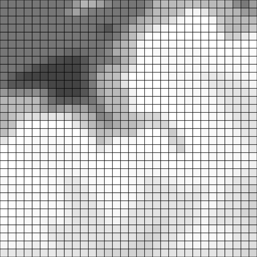
(a)

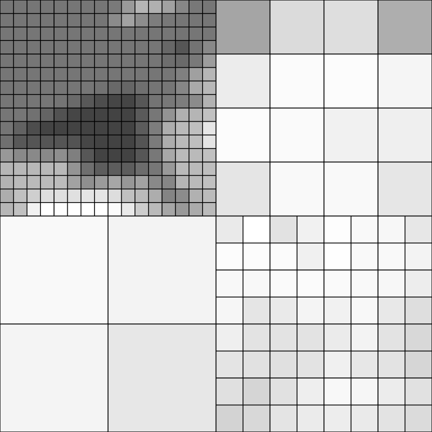
(b)

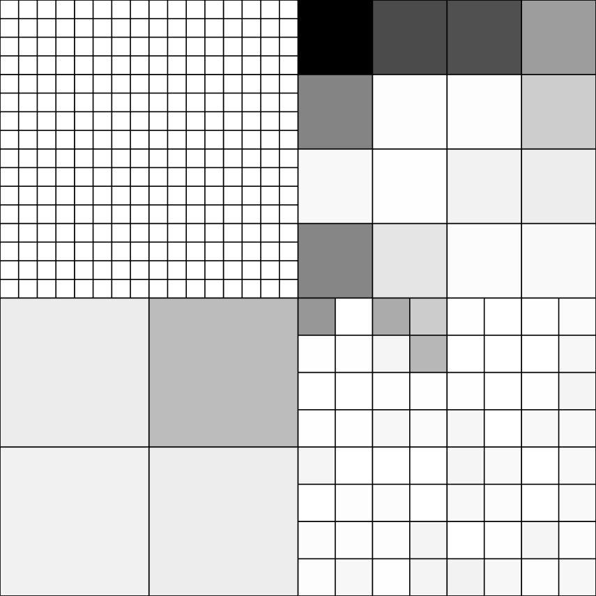
(c)

Figure 1: (a) Finest resolution occupancy grid; (b) Compressed occupancy grid; (c) Variance of the compressed grid, with darker cells indicating higher variance.

We adopt the premise that the environment is represented by a 2D occupancy grid $M$, as proposed in [31, 32] , and with $N$ being the total number of cells in $M$. A robot is equipped with onboard sensors capable of observing a 2D occupancy grid of size $w\times h\leq N$ as shown in Figure 1(1(a)). The vector $x\in\mathbb{R}^{N}$ contains the occupancy values of the grid cells, where the value of the $j$-th component of $x$, denoted by $[x]_{j}$, lies in the range $[0,1]$ for all $j=1,\ldots,N$. Here $[x]_{j}$ represents the traversability of the cell, where $[x]_{j}=1$ indicates a non-traversable cell and $[x]_{j}=0$ denotes an obstacle-free cell.

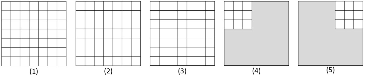
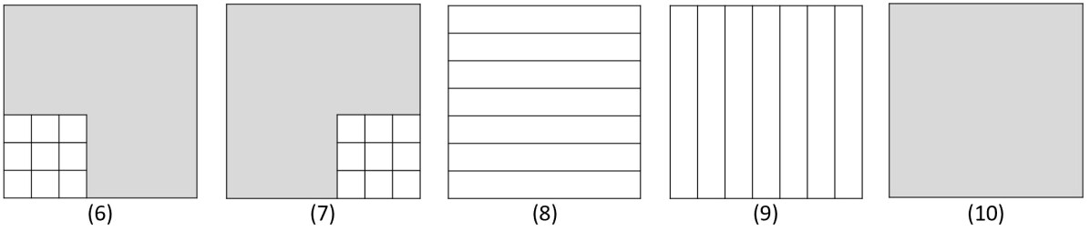
Figure 2: Example of a set of abstractions. The grey area denotes no information.

We define as an abstraction a multi-resolution compressed representation of the occupancy grid, as in Figure 1(1(b)). Each abstraction is characterized by its compression template, indicating how the grid cells are compressed. Examples of a few possible abstractions for a $7\times 7$ grid are shown in Figure 2. Various techniques have been used to determine the occupancy value of a compressed cell [33, 34, 6]. In our previous work [15], we adopted the approach of computing the occupancy value of the compressed cell as the average of the occupancy values of the underlying finest resolution cells. This way, each abstraction can be thought of as a linear mapping ${\mathcal{A}}^{\theta}:[0,1]^{N}\to[0,1]^{k^{\theta}}$, where $k^{\theta}\leq wh\leq N$ is the number of cells in the compressed representation utilizing abstraction ${\theta}$. Specifically, for a given high resolution occupancy map $x\in[0,1]^{N}$, the occupancy values of the cells at abstraction ${\theta}$ are given by $o=\mathcal{A}^{\theta}x$, where $\mathcal{A}^{\theta}\in\mathbb{R}^{k^{\theta}\times N}$. For example, the dimensions in Figure 2 are $w=7$, $h=7$, and the number of compressed cells for abstractions $\theta=8$ and $9$ is $k^{\theta}=7$, while for abstractions $\theta=4,5,6$ and $7$, it is $k^{\theta}=9$, and so forth.

In this study, each compressed cell of an abstraction is assigned a pair of values, the mean and the variance. The communication of the variance among the robots has a two-fold impact. Firstly, it serves as an uncertainty indicator due to the compression. Secondly, it provides better occupancy value estimates along with the mean. To this end, we define the variance $[V]_{i}$ of a compressed cell $i$ as the normalized squared deviation from the mean

$$[V]_{i}=\sum\limits_{j=0}^{N}a_{ij}\left([x]_{j}-[o]_{i}\right)^{2},$$ (1)

where $a_{ij}\triangleq\left[\mathcal{A}^{\theta}\right]_{ij}$. Note that $a_{ij}=0$ if the $j$-th cell is not included in the $i$-th compressed cell and $a_{ij}={1}{/[N^{\theta}]_{i}}$ otherwise, where $[N^{\theta}]_{i}$ is the number of non-zero elements in the $i$-th row of $\mathcal{A}^{\theta}$. Figure 1(1(c)) shows the variance of the compressed occupancy grid presented in Figure 1(1(b)). Darker cells indicate higher variance.

2.1 Communication of Abstracted Environments

Consider a pair of robots, robot $A$ and robot $S$, communicating with each other. At each timestep $t$, robot $S$ chooses an abstraction $\theta_{t}\in\Theta$ to compress its local map and transmits it to robot $A$, where $\Theta=\{1,\ldots,K\}$ is the set of available abstractions (i.e., codebook) that the two robots have agreed upon (e.g., see Figure 2 for a collection of templates). Specifically, robot $S$ transmits the triple $(o_{t},V_{t},{\theta}_{t})$, where $V_{t}$ is the compression variance given in (1), and $o_{t}=\mathcal{A}^{\theta_{t}}x$ with $x$ containing the measurements of robot $S$. Having received the transmitted $\theta_{t}$, robot $A$ computes $\mathcal{A}^{\theta_{t}}$ and attempts to reconstruct $x$ from $o_{t}$ and $V_{t}$.

We denote by $n_{m}$ the number of bits required to transmit the compressed occupancy value $[o]_{i}$ and variance $[V]_{i}$, and $n_{i}$ the number of bits required to transmit an abstraction index ${\theta}$. Hence, the total number of bits $n^{\theta}$ required to transmit the abstracted grid employing abstraction ${\theta}$ is:

$$n^{\theta}=k^{\theta}n_{m}+n_{i}.$$ (2)

3 Problem Formulation

Consider a team of mobile robots with different objectives, navigating through an unfamiliar environment $M\subset\mathbb{R}^{2}$ cluttered with static obstacles. Each robot has its own sensing equipment capable of observing a portion of the environment (local map) as it moves. The team consists of a Seeker robot and multiple mobile Sensors. The Seeker’s goal is to reach a specified target location in minimum time. Meanwhile, the Sensors aim to support the Seeker in achieving its objective by communicating informative abstractions of their local maps to the Seeker at each timestep. The Sensors can be regarded, for example, as surveillance drones capable of moving over ground obstacles, while the Seeker is assumed to be a ground robot, that has to circumnavigate these obstacles.

Let $\textbf{p}_{A,t}$, $\textbf{p}_{s,t}\in M$ be the Seeker and each Sensor’s position, respectively, at timestep $t$, where $s$ denotes the Sensor index, and let $u_{A,t}\in U_{A}$, $u_{s,t}\in U_{S}$ denote the Seeker’s and each Sensor’s control action at time $t$ selected from a finite set of control actions $U_{A}$ and $U_{S}$, respectively.

3.1 Problem Statement

Considering the uncertainty of cell occupancy values caused by compression and given as inputs the initial positions of the Seeker $\textbf{p}_{A,0}$ and Sensors $\textbf{p}_{s,0}$, as well as the Seeker’s destination $\textbf{p}_{A,G}$ and the set of abstractions $\Theta$, we design an exploration strategy for the Sensors to minimize compression uncertainty near the Seeker’s path. Each Sensor communicates to the Seeker the triple $(o_{s,t},V_{s,t},{\theta_{s,t}})$, as detailed in Section 2.1, along with its current position $\textbf{p}_{s,t}$. The Seeker utilizes the variance of each Sensor $V_{s,t}$ to estimate the map compression uncertainty and selects each Sensor’s action $u_{s,t}$ to reduce uncertainty near its path. Our primary goal is for the Seeker to reach its destination in minimum time (shortest path) by using the accumulated measurements to compute its control $u_{A,t}$.

4 Compression Uncertainty

In this section, we quantify the map uncertainty resulting from the unknown environment, and the history of transmitted abstractions $\theta_{0:t}$ until time $t$. The quantified result is represented by a vector $h_{t}\in\mathbb{R}^{N}$, which approximates the uncertainty of each cell in $M$. The Seeker employs $h_{t}$ to compute the trajectories/actions of the Sensors, as elaborated later in Section 5.3.

First, we rewrite (1) as follows

$$x^{\top}\operatorname*{diag}{[\mathcal{A}^{\theta}]_{i}}x=[o]_{i}^{2}+[V]_{i}^{2},$$ (3)

where $\operatorname*{diag}{[\mathcal{A}^{\theta}]_{i}}\in[0,1]^{N\times N}$ is a diagonal matrix with the $i$-th row of $\mathcal{A}^{\theta}$ as its diagonal.

Equation (3) along with $o=\mathcal{A}^{\theta}x$ describe a set in $\mathbb{R}^{N}$ which serves as the estimation domain imposed by abstraction $\theta$. To make the problem computationally tractable and apply convex optimization methods, we relax (3) by replacing the equality with inequality. Hence, a valid estimate $\widehat{x}$ of $x\in[0,1]^{N}$ belongs in the set

$$C^{\theta}=\left\{x\in\mathbb{R}^{N}:\begin{matrix}&x^{\top}\operatorname*{diag}{[\mathcal{A}^{\theta}]_{i}}x\leq[o]_{i}^{2}+[V]_{i}^{2},\hskip 5.0pt&i=1,2,\ldots,k^{\theta}\\ &\mathcal{A}^{\theta}x=o&\\ &0\leq[x]_{j}\leq 1,\hskip 5.0pt&j=1,\ldots,N\end{matrix}\right\}.$$ (4)

Each robot engages in the estimation process individually. A Sensor uses only its own abstractions, while the Seeker utilizes its own measurements and the communicated abstractions from all the Sensors. Considering the history of abstractions $\theta_{s,0:t}$ of the Sensor $s$ up to time $t$, the Sensor’s measurements are described by the set $C_{s,t}=\cap_{\tau=0}^{t}C^{\theta_{s,\tau}}$. The Seeker’s measurement of the $j$-th cell can be described by $\mathcal{\alpha}_{t}^{j}x=o_{t}^{j}$, where $\mathcal{\alpha}_{t}^{j}\in\mathbb{R}^{1\times N}$ has zeros everywhere except at the $j$-th element. Let $C_{A,t}^{\prime}$ be the set containing all the Seeker’s measurements up to time $t$. Then, the Seeker’s accumulated measurements are described by the set $C_{A,t}=\left(\cap_{s\in S}C_{s,t}\right)\cap C^{\prime}_{A,t}$.

Hence, we can now define the compression uncertainty of the $j$-th cell as

$$[\mathcal{H}]_{j}=\max_{x,\widehat{x}\in C_{A,t}}\left|[x]_{j}-[\widehat{x}]_{j}\right|.$$ (5)

If a cell is included in a single compression $i$, then from (4) it follows that $[\mathcal{H}]_{j}=2[\nu]_{i}$ with $[\nu]_{i}^{2}={[N^{\theta}]_{i}}[V]_{i}$. However, as a cell may be included in multiple compressed cells, computing its uncertainty requires considering all the compressed cells within which it is contained. To make the computation of $\mathcal{H}$ tractable, we derive an upper bound, taking into account the abstractions which the cells belong to.

Proposition 4.1.

Let $[x]_{j}$ be the true occupancy value of the $j\text{-th}$ cell and $[\widehat{x}]_{j}$ be any valid estimate of it. Consider also $I$ to be the set of compressed cells of all the abstractions that cell $j$ is a part of. Then,

$$[\mathcal{H}]_{j}\leq[h]_{j},$$ (6a)

$$[h]_{j}=\min\limits_{i\in I}\!\left\{[\nu]_{i}+[o]_{i}\right\}+\min\limits_{i\in I}\!\left\{[\nu]_{i}-[o]_{i}\right\}.$$ (6b)

Proof 4.2.

From Equation (1)

$$\left|[x]_{j}-[o]_{i}\right|\leq[\nu]_{i},\qquad\forall i\in I,$$ (7)

where recall that $[\nu]_{i}^{2}={[N^{\theta}]_{i}}[V]_{i}$. Equivalently,

$$\max\limits_{i\in I}\!\left\{[o]_{i}-[\nu]_{i}\right\}\leq[x]_{j}\leq\min\limits_{i\in I}\!\left\{[o]_{i}+[\nu]_{i}\right\}.$$ (8)

A valid estimate $[\widehat{x}]_{j}$ of $[x]_{j}$ must also satisfy

$$\max\limits_{i\in I}\!\left\{[o]_{i}-[\nu]_{i}\right\}\leq[\widehat{x}]_{j}\leq\min\limits_{i\in I}\!\left\{[o]_{i}+[\nu]_{i}\right\},$$ (9)

since the true occupancy value lies in this range. Combining (8) and (9), we obtain

$$[\mathcal{H}]_{j}\leq[h]_{j},$$

where,

$$[h]_{j}=\min\limits_{i\in I}\!\left\{[o]_{i}+[\nu]_{i}\!\right\}-\max\limits_{i\in I}\!\left\{[o]_{i}-[\nu]_{i}\right\},$$

which is equivalent to (6).

5 Framework Architecture

In this section, we introduce the proposed framework, depicted in Figure 3. The framework leverages the same Decoder and Path Planner as in [15].

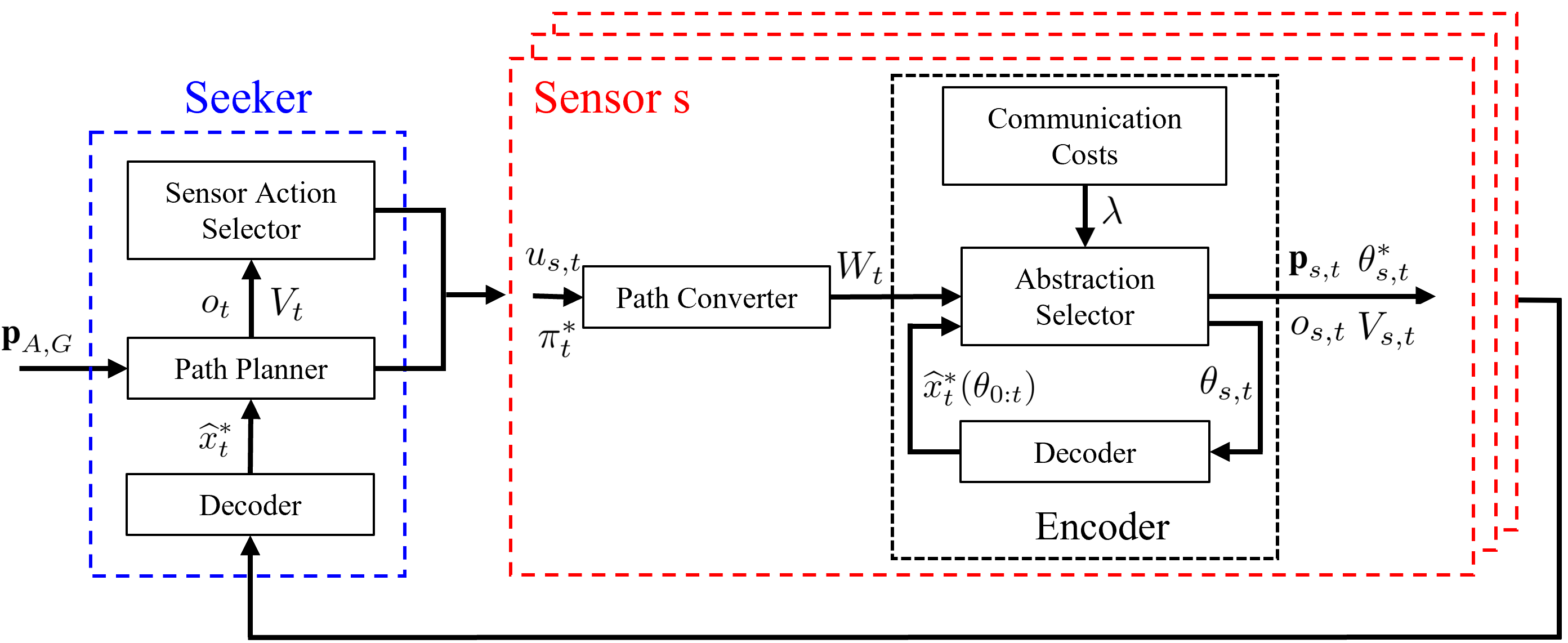
Figure 3: Flowchart of the proposed framework’s architecture at timestep $t$. The Seeker shares its current optimal path $\pi^{*}_{t}$ to the Sensors along with their actions $u_{s,t}$. The Sensors utilize this to select the optimal abstraction of their respective local maps $\theta^{*}_{s,t}\in\Theta$ and send it to the Seeker to aid in reaching its target.

5.1 Decoder

The decoder (see Figure 3) generates estimates for $x\in[0,1]^{N}$, representing the occupancy of cells. Each robot utilizes its own constraint set $C_{t}$ to compute its estimates ($C_{A,t}$ for Seeker and $C_{s,t}$ for Sensor $s$). Hence, the estimation vector is given by

$$\widehat{x}^{*}_{t}=\operatorname*{arg\,min}_{\widehat{x}_{t}\in C_{t}}\|\widehat{x}_{t}-\mbox{$\frac{1}{2}$}\mathbf{1}\|^{2},$$ (10)

where we assume that $x$ follows a known distribution with mean $\mathbb{E}[[x]_{j}]=0.5$. The intuition for this choice and the proof can be found in [15].

5.2 Path Planner

Consider the graph $\mathcal{G}=(\mathcal{N}$, $\mathcal{E}$) associated with the discretized map $M$, where $\mathcal{N}$ represents the set of vertices and $\mathcal{E}$ the set of edges. With a slight abuse of notation, we denote both the cell positions in $M$ and the graph vertices $\mathcal{N}$ as p, since they coincide. An edge connects two vertices if the Seeker can move between them using a control action $u_{A}\in U$. We assume that the traversal time of a cell is proportional to its occupancy value (difficulty to traverse) plus a constant (penalty for movement). The cost of traversing a vertex is given by [15, 35]

$$c_{\epsilon}(\textbf{p})=\begin{cases}x_{\textbf{p}}+a,&\text{if $\textbf{p}\in P_{\epsilon}$},\\ N(\epsilon+a),&\text{otherwise},\end{cases}$$ (11)

where $x_{\textbf{p}}\in[0,1]$ is the occupancy value of the cell at position p, $a$ is a constant penalty for movement, and $P_{\epsilon}=\{\textbf{p}\in\mathcal{N}:x_{\textbf{p}}\leq\epsilon\}$ is the set of cells meeting a feasibility condition, with $\epsilon\in[0,1]$ denoting the threshold for considering a cell to be an obstacle.

Utilizing (11), the Seeker’s optimal path is given by

$$\pi^{*}=\operatorname*{arg\,min}_{\pi\in\Pi}\sum_{\textbf{p}\in\pi}{c_{\epsilon}(\textbf{p})},$$ (12)

where $\Pi$ is the set of paths with the first element being the Seeker’s position at timestep $t$, denoted by $\textbf{p}_{A,t}$, and the last element being its goal location $\textbf{p}_{A,G}$.

Figure 4(4(a)) presents an example of an occupancy grid with obstacles, while Figure 4(4(b)) illustrates the associated graph with the Seeker’s optimal path (computed, for instance, using Dijkstra’s graph search algorithm [36]).

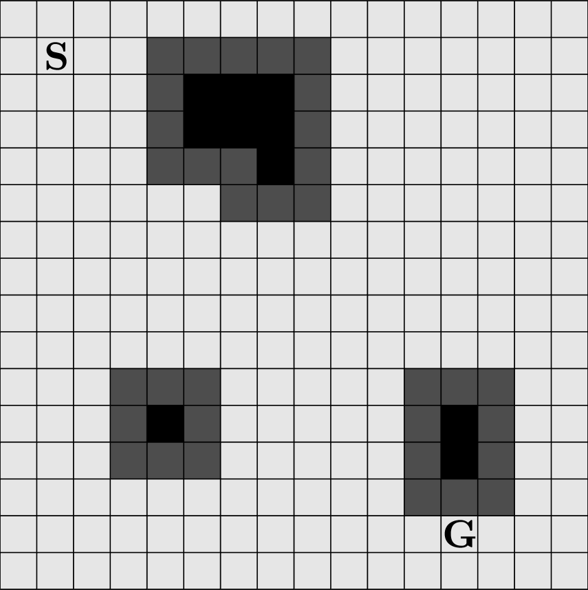
(a)

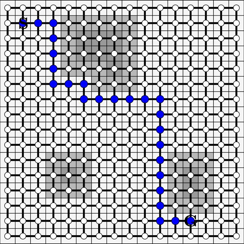
(b)

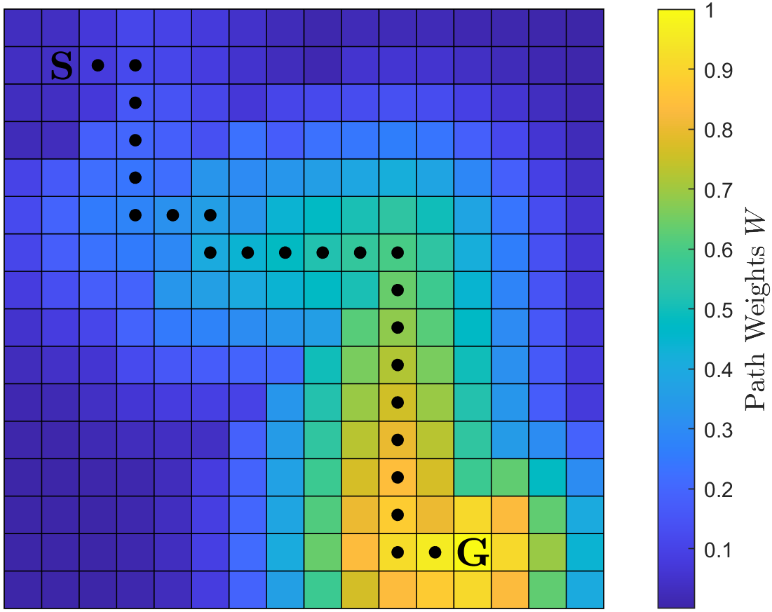
(c)

Figure 4: (a) Example of a discretized environment. S denotes the starting cell while G denotes the target; (b) Associated graph of the environment employing the set of actions $U=$ {UP, DOWN, LEFT, RIGHT}, along with the optimal path (blue nodes) with cost function (11); (c) Path weights computed using (13).

5.3 Sensor Action Selector

The Sensors’ actions are selected to minimize the Seeker’s compression uncertainty. To accomplish this, their actions are selected based on a task-driven metric for uncertainty, denoted by $R_{t}\in\mathbb{R}^{N}$. This metric relies on the current Seeker’s path $\pi^{*}_{t}$ and the uncertainty of the whole map. In this study, the Sensors’ actions are selected by the Seeker in a centralized manner (see Figure 3). A decentralized approach can be applied, in the case of a single Sensor or given that the Sensors share their measurements among themselves.

To compute $R_{t}$, first we construct an area of interest around $\pi^{*}_{t}$ by assigning weights to each cell within $M$. Given that the Seeker will likely explore the vicinity of its current position in subsequent timesteps, and that its path may vary in the future, it is more advantageous for the Sensors to prioritize exploration in the vicinity of the Seeker’s target. Hence, the weight of each cell is given by

$$w_{t}(\textbf{p})=\frac{|\pi_{d}|}{|\pi^{*}_{t}|}e^{-\frac{d^{2}}{2v}},$$ (13a)

$$d=\min\limits_{\textbf{p}_{\pi}\in\pi^{*}_{t}}\|\textbf{p}-\textbf{p}_{\pi}\|,$$ (13b)

where $\textbf{p}\in M$, $v$ is a parameter characterizing the width of the region of interest around the path, $|\pi^{*}_{t}|$ is the total number of nodes (length) in $\pi^{*}_{t}$, and $|\pi_{d}|$ is the length of the portion of $\pi^{*}_{t}$, starting from the current location $\textbf{p}_{A,t}$ up to the argument of minimization of (13b). Figure 4(4(c)) depicts these path weights.

Hence, we define the task-driven metric of uncertainty $R_{t}$ as follows

$$R_{t}=W_{t}\circ h_{t},$$ (14)

where $W_{t}\in\mathbb{R}^{N}$ contains the weights $w_{t}(\textbf{p})$ of every cell computed by (13), $\circ$ is the Hadamard product, and $h_{t}\in\mathbb{R}^{N}$ contains the uncertainty given by (6).

The action of each Sensor is computed by solving an infinite-horizon discounted Markov Decision Process (MDP) $\langle\mathcal{M}_{s},U_{S},\widetilde{R}_{s,t},\gamma,p\rangle$ at each timestep $t$. Here, $\mathcal{M}_{s}$ represents the set of states, where each state corresponds to a possible local map of the Sensor s, denoted by $L_{s}$, and $U_{S}$ is the set of actions. To provide a tractable and computationally efficient solution, we restrict the states to the neighborhood around the Sensor’s current local map. Let $l$ be the radius of that neighborhood and $N^{\prime}\leq N$ be the number of states.

The reward vector $\widetilde{R}_{s,t}\in\mathbb{R}^{N^{\prime}}$ is defined as the sum of rewards obtained at each position p within the Sensor’s local map, given by

$$[\widetilde{R}_{s,t}]_{L_{s}}=\sum\limits_{\textbf{p}\in L_{s}}R_{t}(\textbf{p}).$$ (15)

Moreover, $\gamma\in(0,1)$ stands for the discount factor, and $p:\mathcal{M}_{s}\times\mathcal{M}_{s}\times U_{S}\to\{0,1\}$ is the transition function with transition matrix $P_{s}\in\mathbb{R}^{N^{\prime}\times N^{\prime}}$.

The value function is defined as

$$\mathcal{V}_{s,t}(\mu_{s})=\sum_{\tau=0}^{\infty}\gamma^{\tau}P_{s}^{\tau}(\mu_{s})\widetilde{R}_{s,t},$$ (16)

where $\mu_{s}$ denotes the policy transitioning from a state $L_{s}$ to another state $L_{s}^{\prime}$. Therefore, we obtain the optimal policy $\mu_{s}^{*}=\operatorname*{arg\,max}_{\mu_{s}}\mathcal{V}_{s,t}(\mu_{s})$, and each sensor’s action at each timestep $t$

$$u_{s,t}=\mu_{s}^{*}(L_{s,t}),$$ (17)

where $L_{s,t}$ is the local map of the Sensor $s$ being in position $\textbf{p}_{s,t}$.

Algorithm 1 The Sensor Action Selector’s Algorithm

Input: $\pi^{*}_{t}$, $\mathcal{A}_{0:t}$, $o_{0:t}$, $V_{0:t}$, $\textbf{p}_{S}$, $l$, $U_{S}$, $\gamma$, $p$
      Output: $u_{S,t}$

1:$h_{t}\leftarrow$ Uncertainty$(\mathcal{A}_{0:t},o_{0:t},V_{0:t})$ using (6)

2:$W_{t}\leftarrow$ Weights$(\pi^{*}_{t})$ using (13)

3:$R_{t}\leftarrow$ TDUncertainty$(h_{t},W_{t})$ using (14)

4:$S_{prev}\leftarrow\emptyset$

5:for all $s\in S$ do

6:     $\mathcal{M}_{s}\leftarrow\textsc{States}(\textbf{p}_{s},l)$

7:     $\widetilde{R}_{s,t}\leftarrow\textsc{Reward}(\mathcal{M}_{s},R_{t})$ using (15)

8:     $\widetilde{R}_{s,t}\leftarrow\textsc{Overlapping}(\widetilde{R}_{s,t},\mathcal{M}_{s\in S_{prev}})$

9:     $u_{s,t}\leftarrow\textsc{MDP}(\mathcal{M}_{s},U_{S},\widetilde{R}_{s,t},\gamma,p)$

10:     $S_{prev}\leftarrow S_{prev}\cup\{s\}$

11:end for

12:return $u_{S,t}$

The algorithm for selecting the Sensors’ actions is outlined in Algorithm 1. Lines 5-11 iteratively compute the action for each sensor by solving the individual MDPs. Note that Line 8 sets the rewards to zero for the states already considered by Sensors whose actions were determined in previous iterations, thus preventing overlap. Line 9 performs Value Iteration.

5.4 Path Converter

The Seeker sends its current optimal path $\pi^{*}_{t}$ obtained from (12) to the Sensors. Then, each Sensor utilizes this information to guide its abstraction selection process separately. This is achieved by constructing $W_{t}$ using (13).

5.5 Encoder

A Sensor’s encoder selects the optimal abstraction from the given set $\Theta$, to transmit to the Seeker. Let $\theta_{s}\in\Theta$ denote the Sensor’s $s$ abstraction. For the rest of this section, we will omit the index $s$ for simplicity. Given the past selection $\theta_{0:t-1}$, the optimal abstraction at $t$ is derived through the minimization of the following criterion

$$J_{t}(\theta_{t})=\beta D_{t}+(1-\beta)H_{t}+\lambda(\theta_{t}),$$ (18a)

$$D_{t}=\|W_{t}\circ(\widetilde{x}_{t}-\widehat{x}_{t}^{*}(\theta_{0:t}))\|^{2},\quad H_{t}=\|W_{t}\circ h_{t}(\theta_{0:t})\|^{2},\quad$$ (18b)

$$\theta^{*}_{t}=\operatorname*{arg\,min}\limits_{\theta_{t}\in\Theta}J_{t}(\theta_{t}),$$ (18c)

where $\beta\in[0,1]$ is a trade-off factor, $\widetilde{x}_{t}\in\mathbb{R}^{N}$ is the sensed occupancy values by each Sensor until time $t$, $\widehat{x}_{t}(\theta_{0:t})\in\mathbb{R}^{N}$ is the estimation vector, $h_{t}(\theta_{0:t})$ is the uncertainty vector given by (6), and $\lambda(\theta_{t})$ is the communication cost (related to $n^{\theta}$ in (2)). It is important each Sensor to select the optimal abstraction for the specific Seeker’s decoder (see Figure 3). Hence, the estimation vector $\widehat{x}_{t}(\theta_{0:t})$ is computed using (10) with the constraint set $C_{s,t}$.

6 Experiments

Two different scenarios were studied in a $64\times 64$ environment (see Figure 5(5(a))). In the first scenario, we compared our proposed algorithm for different values of the parameter $l$ of the MDP neighborhood (See Section 5.3) to the algorithm introduced in [15]. We also present the results of a greedy algorithm, which determines the next state by choosing the Sensor’s action with the highest immediate reward from the set $U_{S}=${UP, DOWN, LEFT, RIGHT}. The simulations involved a single Sensor. In the second scenario, we tested different parameters $l$ of our proposed algorithm by conducting simulations with three Sensors. In both scenarios, we performed 100 simulations with varied Sensors’ initial positions. All the robots initiated movement simultaneously, traversing one cell per timestep. The Sensors have the ability to move over obstacles (e.g., surveillance drones).

The Seeker’s sensing region is a $5\times 5$ grid around its position, while the Sensors have a field of view of $7\times 7$. The Seeker’s initial position is $\textbf{p}_{A,0}=(6,29)$ and its target position is $\textbf{p}_{A,G}=(43,25)$. The Seeker’s Path Planner parameters in (11) are $a=0.025$ and $\epsilon=0.501$, the parameter in (13) is $v=10$, and the discount factor in (16) is $\gamma=0.9$. The Sensors’ encoders utilize a finite set of 10 abstractions, as shown in Figure 2, where the parameters in (18) are $\beta=0.9$ and $\lambda(\theta)=0.05k^{\theta}$, where the cost of abstraction is proportional to the amount of bits required for transmitting the abstracted map.

6.1 Performance Metrics

We assumed that the time needed to traverse a cell for the Seeker is proportional to the cell’s occupancy value (see Section 5.2). Let $\pi_{f}$ include the cells that Seeker traversed to reach its goal, without excluding duplicate cells. Then, the accumulated cost/time is $\mathcal{C}=\sum_{\textbf{p}\in\pi_{f}}{c_{\epsilon}(\textbf{p})}$ and the average time ratio is

$$r_{\textrm{time}}=\frac{1}{n_{\textrm{sim}}}\sum_{i=0}^{n_{\textrm{sim}}}\frac{\mathcal{C}_{1}(i)}{\mathcal{C}_{2}(i)},$$ (19)

where $n_{\textrm{sim}}=100$ is the total simulation number, $\mathcal{C}_{1}(i)$, and $\mathcal{C}_{2}(i)$ are the accumulated costs of the proposed and the compared framework, respectively, at simulation $i$. The compared framework varies depending on the Scenario.

We also compute the average ratio of the transmitted bits

$$r_{\textrm{bits}}=\frac{1}{n_{\textrm{sim}}}\sum_{i=0}^{n_{\textrm{sim}}}\frac{\sum_{t=0}^{T_{1}(i)}{n_{1,t}}(i)}{\sum_{t=0}^{T_{2}(i)}{n_{2,t}}(i)},$$ (20)

where $n_{j,t}(i)$, for $j\in\{1,2\}$ is given in (2) and denotes the bits sent by each framework’s Sensors at $t$ and simulation $i$, with $n_{m}$ divided by two if the variance is not transmitted. We set $n_{m}=24$, and $n_{i}=4$. $T_{j}(i)$ is the number of Sensors’ steps, which is fixed to 60 for all the simulations (as also done in [15]).

6.2 Comparison with [15]

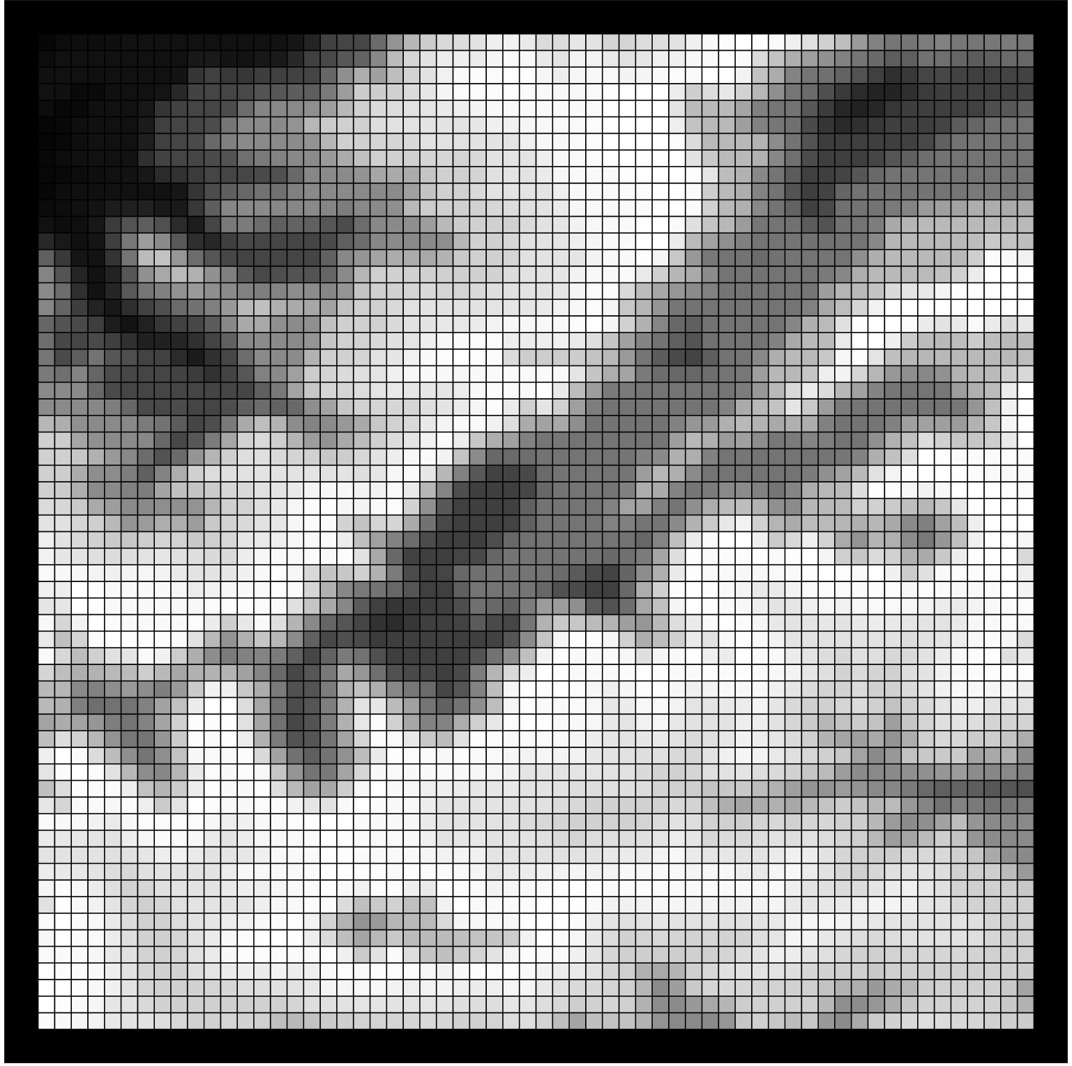
(a)

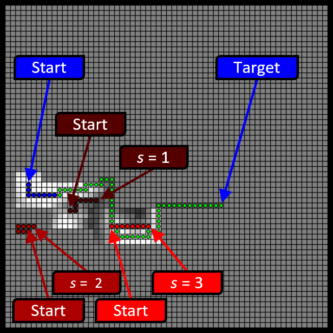
(b)

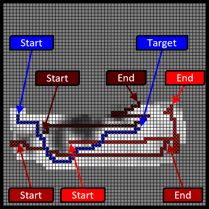
(c)

Figure 5: (a) Simulation Environment; (b-c) Simulation snapshot at the timestep $t=8$ (b) and $t=61$ (c) using the proposed exploration framework ($l=10,\textbf{p}_{1,0}=(14,24),\textbf{p}_{2,0}=(6,21),\textbf{p}_{3,0}=(22,21)$). The Seeker’s path until $t$ is presented in blue, its predicted path with green, while the Sensors’ trajectories in red.

Table 1: Simulation results for Scenario 1

	Greedy	$l=1$	$l=2$	$l=10$	FI in [15]
$r_{\textrm{time}}$	0.853	0.837	0.847	0.880	0.794
$r_{\textrm{bits}}$	5.835	5.990	6.029	6.259	8.131

In the first scenario, we varied the Sensor’s initial position. For the compared framework, we simulated two different pre-defined paths and took the average of them to compute the cost $\mathcal{C}_{2}$ and bits $\sum_{t=0}^{T_{2}(i)}{n_{2,t}}$ of the simulations. The paths followed a square trajectory (as in [15]) with one path traversing the square clockwise and the other counterclockwise. In the proposed framework, to ensure a fair comparison with the other framework and given that we are employing only one Sensor, we avoided the transmission of variance and relocated the Sensor Action Selector (see Figure 3) from the Seeker to the Sensor.

The resulting average time ratio and bit ratio are presented in Table 1. The results indicate that all frameworks effectively reduces the time required for the Seeker to reach its target compared to the framework in [15], albeit at the expense of increased bits. Moreover, we can conclude that the Sensor’s action selection based on the MDP outperforms the greedy strategy, although the parameter $l$ must be carefully selected, depending on the field of view of the Sensor and the number of Sensors. Note that the last column of Table 1 corresponds to the Fully-Informed framework in [15]. We conclude that while this framework does incur a lower cost, it achieves this by necessitating a greater number of bits and relies on a pre-defined Sensor path that is manually crafted.

6.3 MDP Neighborhood

In this scenario, we tested our exploration algorithm for different values of the MDP neighborhood parameter $l$. We varied the initial positions of the three employed Sensors. We transmit the variance to the Seeker to compute the Sensors’ actions. Framework No. 1 corresponds to $l=10$, and No. 2 to $l=1$ in equations (19) and (20).

The resulting ratios are $r_{\textrm{time}}=1.11$ and $r_{\textrm{bits}}=1.00$, indicating that setting $l=1$ yields slightly better results, similar to Scenario 1. However, setting $l=10$ increases the exploration coverage of the map, since $l$ determines the maximum distance between the Sensors (as indicated by Line 8 in Algorithm 1), which is particularly beneficial for larger maps and numerous Sensors. This can be observed in Figures 5(5(b)) - (5(c)) where a simulation with $l=10$ is shown. Note that Figure 5(5(b)) is the timeframe before the Seeker corrects its computed path.

7 Conclusions

In this paper, we studied the problem of exploring unknown environments with mobile sensors that communicate compressed measurements. The sensors are deployed to facilitate mobile robot path-planning. We introduce a novel communication framework along with a tractable multi-agent exploration algorithm aimed at optimizing the actions of the sensors. Our algorithm leverages a task-driven measure of compression uncertainty, as a reward function. Simulation results demonstrate the effectiveness of our framework in reducing the time required for the robot to reach its target without excessively burdening the communication network. Future extensions will be focused on refining the proposed framework by incorporating a more sophisticated abstraction selection search method to decrease the computational time of the Sensors.

References

- [1] H. Sugiyama, T. Tsujioka, M. Murata, Collaborative movement of rescue robots for reliable and effective networking in disaster area, in International Conference on Collaborative Computing: Networking, Applications and Worksharing (San Jose, CA, 2005)
- [2] O. Salzman, R. Stern, Research challenges and opportunities in multi-agent path finding and multi-agent pickup and delivery problems, in 19th International Conference on Autonomous Agents and MultiAgent Systems (Auckland, New Zealand, 2020), pp. 1711–1715
- [3] S.B. Kesner, J.S. Plante, P.J. Boston, T. Fabian, S. Dubowsky, Mobility and power feasibility of a microbot team system for extraterrestrial cave exploration, in IEEE International Conference on Robotics and Automation (ICRA) (Rome, Italy, 2007), pp. 4893–4898
- [4] J. Gielis, A. Shankar, A. Prorok, A critical review of communications in multi-robot systems. Current Robotics Reports 3(4), 213–225 (2022)
- [5] Z. Xu, V. Tzoumas, Resource-aware distributed submodular maximization: A paradigm for multi-robot decision-making, in IEEE 61st Conference on Decision and Control (CDC) (Cancun, Mexico, 2022), pp. 5959–5966
- [6] D.T. Larsson, D. Maity, P. Tsiotras, Q-tree search: An information-theoretic approach toward hierarchical abstractions for agents with computational limitations. IEEE Transactions on Robotics 36(6), 1669–1685 (2020)
- [7] C. Hireche, C. Dezan, J.P. Diguet, L. Mejias, BFM: A scalable and resource-aware method for adaptive mission planning of UAVs, in IEEE International Conference on Robotics and Automation (ICRA) (Brisbane, QLD, Australia, 2018), pp. 6702–6707
- [8] M.H. Mamduhi, D. Maity, K.H. Johansson, J. Lygeros, Regret-optimal cross-layer co-design in networked control systems–part I: General case. IEEE Communications Letters 27(11), 2874–2878 (2023)
- [9] D. Maity, M.H. Mamduhi, J. Lygeros, K.H. Johansson, Regret-optimal cross-layer co-design in networked control systems–part II: Gauss-Markov case. IEEE Communications Letters 27(11), 2879–2883 (2023)
- [10] M.H. Mamduhi, D. Maity, S. Hirche, J.S. Baras, K.H. Johansson, Delay-sensitive joint optimal control and resource management in multiloop networked control systems. IEEE Transactions on Control of Network Systems 8(3), 1093–1106 (2021)
- [11] D.F. Delchamps, Stabilizing a linear system with quantized state feedback. IEEE Transactions on Automatic Control 35(8), 916–924 (1990)
- [12] R.W. Brockett, D. Liberzon, Quantized feedback stabilization of linear systems. IEEE Transactions on Automatic Control 45(7), 1279–1289 (2000)
- [13] G.N. Nair, R.J. Evans, Stabilizability of stochastic linear systems with finite feedback data rates. SIAM Journal on Control and Optimization 43(2), 413–436 (2004)
- [14] V. Kostina, B. Hassibi, Rate-cost tradeoffs in control. IEEE Transactions on Automatic Control 64(11), 4525–4540 (2019)
- [15] E. Psomiadis, D. Maity, P. Tsiotras, Communication-aware map compression for online path-planning, in IEEE International Conference on Robotics and Automation (ICRA) (Yokohama, Japan, 2024)
- [16] R. Marcotte, X. Wang, D. Mehta, E. Olson, Optimizing multi-robot communication under bandwidth constraints. Autonomous Robots 44(1), 43–55 (2020)
- [17] V. Unhelkar, J. Shah, Contact: Deciding to communicate during time-critical collaborative tasks in unknown, deterministic domains, in AAAI Conference on Artificial Intelligence (Phoenix, AZ, 2016)
- [18] M. Fu, Lack of separation principle for quantized linear quadratic gaussian control. IEEE Transactions on Automatic Control 57(9), 2385–2390 (2012)
- [19] S. Yüksel, A note on the separation of optimal quantization and control policies in networked control. SIAM Journal on Control and Optimization 57(1), 773–782 (2019)
- [20] D. Maity, P. Tsiotras, Optimal controller synthesis and dynamic quantizer switching for linear-quadratic-Gaussian systems. IEEE Transactions on Automatic Control 67(1), 382–389 (2022)
- [21] D. Maity, P. Tsiotras, Optimal quantizer scheduling and controller synthesis for partially observable linear systems. SIAM Journal on Control and Optimization 61(4), 2682–2707 (2023)
- [22] A. Krause, A. Singh, C. Guestrin, Near-optimal sensor placements in gaussian processes: Theory, efficient algorithms and empirical studies. Journal of Machine Learning Research 9, 235–284 (2008)
- [23] B. Mu, A.a. Agha-mohammadi, L. Paull, M. Graham, J. How, J. Leonard, Two-stage focused inference for resource-constrained collision-free navigation, in Robotics: Science and Systems Conference (Rome, Italy, 2015)
- [24] E. Paraskevas, D. Maity, J.S. Baras, Distributed energy-aware mobile sensor coverage: A game theoretic approach, in American Control Conference (ACC) (Boston, MA, USA, 2016), pp. 6259–6264
- [25] D. Maity, J.S. Baras, Dynamic, optimal sensor scheduling and value of information, in 18th International Conference on Information Fusion (Washington, DC, USA, 2015), pp. 239–244
- [26] M.A. Demetriou, I.I. Hussein, Estimation of spatially distributed processes using mobile spatially distributed sensor network. SIAM Journal on Control and Optimization 48(1), 266–291 (2009)
- [27] J. Fang, H. Zhang, R.V. Cowlagi, Interactive route-planning and mobile sensing with a team of robotic vehicles in an unknown environment, in AIAA Scitech 2021 Forum (2021)
- [28] F. Bourgault, A. Makarenko, S. Williams, B. Grocholsky, H. Durrant-Whyte, Information based adaptive robotic exploration, in IEEE/RSJ International Conference on Intelligent Robots and Systems (Lausanne, Switzerland, 2002)
- [29] A. Asgharivaskasi, N. Atanasov, Semantic octree mapping and Shannon mutual information computation for robot exploration. IEEE Transactions on Robotics 39(3), 1910–1928 (2023)
- [30] B. Charrow, S. Liu, V. Kumar, N. Michael, Information-theoretic mapping using Cauchy-Schwarz quadratic mutual information, in IEEE International Conference on Robotics and Automation (ICRA) (Seattle, WA, USA, 2015), pp. 4791–4798
- [31] A. Elfes, Sonar-based real-world mapping and navigation. IEEE Transactions on Robotics and Automation 3(3), 249–265 (1987)
- [32] H.P. Moravec, Sensor fusion in certainty grids for mobile robots. AI Magazine 9(2), 61–74 (1988)
- [33] R.V. Cowlagi, P. Tsiotras, Multiresolution motion planning for autonomous agents via wavelet-based cell decompositions. IEEE Transactions on Systems, Man, and Cybernetics, Part B (Cybernetics) 42(5), 1455–1469 (2012)
- [34] G.K. Kraetzschmar, G.P. Gassull, K. Uhl, Probabilistic quadtrees for variable-resolution mapping of large environments. IFAC Proceedings Volumes 37(8), 675–680 (2004)
- [35] D.T. Larsson, D. Maity, P. Tsiotras, Information-theoretic abstractions for planning in agents with computational constraints. IEEE Robotics and Automation Letters 6(4), 7651–7658 (2021)
- [36] E.W. Dijkstra, A note on two problems in connexion with graphs. Numerische Mathematik 1(1), 269–271 (1959)