Non-resonant invariant foliations of quasi-periodically forced systems
Abstract
We show the existence and uniqueness of invariant foliations about invariant tori in analytic discrete-time dynamical systems. The parametrisation method is used prove the result. Our theory is a foundational block of data-driven model order reduction, that can only be carried out using invariant foliations. The theory is illustrated by two mechanical examples, where instantaneous frequencies and damping ratios are calculated about the invariant tori.
School of Engineering Mathematics and Technology, University of Bristol, Ada Lovelace Building, Tankard’s Close, Bristol BS8 1TW, email: r.szalai@bristol.ac.uk
Keywords
Invariant foliation, invariant manifold, parametrisation method, reduced order model
MSC codes
34A34 34C45 37M21 37C86
1 Introduction
It was found after an exhaustive review of possible ROM representations that invariant foliations are the only mathematical structure that can be fitted to existing data [24]. The theory of invariant foliations is intertwined with that of invariant manifolds [21]. Historically, stable, unstable and centre manifolds and otherwise normally-hyperbolic invariant manifolds were at the focus of investigation [17, 11, 18, 29]. Later, it was found that hyperbolicity can also be achieved in a nonlinear coordinate systems about an invariant object, which led to non-resonant invariant manifolds [9]. The parametrisation method was introduced to provide a comprehensive theoretical framework and prove existence and uniqueness of non-resonant invariant manifolds under general circumstances, for example in infinite dimensions [5, 6]. Moreover, the parametrisation method proved to be successful in inspiring numerical techniques [15, 27, 14] to calculate invariant manifolds. The parametrisation method is similar to normal form theory [28], which also considers non-resonant terms.
Invariant foliations received less attention and the focus was mainly on stable and unstable foliations near stable and unstable manifolds, sometimes bundled together with the centre manifold [3, 2]. Non-resonant invariant foliations about periodic points were shown to exist and unique in [23]. Invariant foliations may exist under less restrictive circumstances. Given their potential to obtain data-driven reduced order models (ROM), exploring such situations is warranted. In this paper we explore the case of quasi-periodic systems and the existence of invariant foliations about invariant tori. The theory follows a similar approach to [16], in that we use the parametrisation method to describe the geometry of the foliation and the Kantorovich-Newton theorem to prove its existence and uniqueness.
Koopman eigenfunctions that correspond to point spectra also describe foliations [19]. The Koopman operator is globally defined, hence does not require the existence of a periodic or quasi-periodic orbit. The drawback of the Koopman approach is that the dynamics on the invariant foliation is assumed to be linear. Whenever the dynamics is not linearisable, continuous spectrum occurs [20]. The numerical treatment of the continuous spectrum requires careful attention [8], and it is not clear that accounting for a large number of spectral points still leads to a ROM. We also note that being linearisable is a generic property, and as we can see from our examples, some nonlinear phenomena can be recovered from seemingly linear systems if we consider the nonlinear frame they are defined in.
We also note that uniqueness results are local and numerically fragile. Under most circumstances, there is a family of invariant manifolds/foliations that satisfy the invariance equations, so we need a constraint that singles one out. The parametrisation method [5] uses smoothness as a deciding factor, while exponential rates can also be used [10], at least for pseudo-stable manifolds. As was pointed out in [9], the two definitions may not lead to the same result. From the perspective of applications, smoothness of a manifold is very difficult to establish, especially when data is involved.
While the present paper is restricted to the neighbourhood of quasi-periodic tori, the direction of travel for our investigation is to extend the theory of invariant foliations to a large class of systems, preferably with multiple (complex) attractors.
The structure of the paper is the following. We first describe the set-up for our analysis, which includes a quick review of exponential dichotomies for non-autonomous systems. The second section states and proves our theorem about the existence and uniqueness of invariant foliations for quasi-periodically forced systems. The third section details the numerical methods to calculate the foliation, which is necessary, given that there is significant difference between the theoretical results and the discretised solution of the invariance equation. Finally, in the fourth section, we illustrate our results through two examples. The appendix includes known results about the existence of invariant tori and we recall the Kantorovich-Newton theorem for completeness.
1.1 Problem setting
We assume a deterministic and discrete-time system in the form of
| (1) |
where , , is an analytic function, is an -dimensional inner product vector space, is the -dimensional torus and is a constant angle of rotation on the torus. We also assume an invariant torus
| (2) |
where is an analytic function and satisfies the invariance equation
| (3) |
The linear dynamics about the invariant torus holds a key to finding invariant foliations. Therefore we define
and consider the system
| (4) |
The phase space of (4), denoted by is called the trivial vector bundle. The decomposition of is a Whitney sum of sub-bundles, . Each sub-bundle is composed of fibres, which means that for each , is a subspace of , and therefore . Note that the same decomposition can be defined for the adjoint trivial bundle , as well. For the sub-bundles to be meaningful they need to be invariant under equation (4), which means that for each fibre we must have
| (5) |
or for the adjoint sub-bundle,
| (6) |
In order to make the calculations of invariant vector bundles computationally accessible, we represent them by families of orthogonal matrices. The two invariance equations (5), (6) can be condensed into one, if we use a projection , in which case and . The invariance equation for the projection is
| (7) |
A projection can be factored into a product , where is an orthogonal operator having the same range as and therefore . Due to being a projection, we also have . Substituting the factorisation of into invariance equation (7) produces
| (8) |
Multiplying (8) by from the left yields
| (9) |
where and multiplying (8) by from the right yields
| (10) |
Equations (9) and (10) are precursors to the invariance equations of foliations and manifolds. One can also think of equations (9) and (10) as generalisations for eigenvalues and eigenvectors, where takes the place of the eigenvalue, the right eigenvector and the left eigenvector.
Invariance alone is not sufficient to characterise the linear dynamics, we also need a dynamic property that decides how to split up the linear system (4). This notion is the exponential dichotomy, which has been introduced in [22] for non-autonomous systems, though similar notions were used before.
Definition 1.
Given a projection , satisfying the invariance equation (7), we say that there is an exponential dichotomy for a positive real number if there exists such that for all and all the inequalities hold
The set of values for which there exists an exponential dichotomy is called the resolvent set and denoted by . The complement is called the dichotomy spectrum of system (4).
Remark 2.
Matrix only needs to be invertible on the range of . This allows us to have and arbitrarily small .
Corollary 3.
Equation
where and are analytic has a unique solution within the set of analytic functions if .
Proof.
We use a contraction mapping argument. The space is separated into two by the projection . On the range of we use the iteration , while on the range of , we use the iteration
to find a convergent solution. ∎
There are a few properties of the resolvent set or the spectrum that we need to use. These properties are widely described in the literature, in particular [1, 22]. The resolvent set consists of a finite number of open intervals, which we denote by
| (11) | |||
with ordering and , such that . Note that the maximum is . Within a resolvent interval for , the invariant projection is independent of and therefore can be denoted by , where . We can also create spectral intervals
| (12) | ||||
| (13) |
that are sometimes just points. The full spectrum then becomes . Note that if is an invariant projection, so is . We also have the inclusions
| (14) |
and therefore . The inclusions can be used to decompose the system (4) into the same number of subsystems as there are spectral intervals. We can then define the spectral projections by
which are similarly invariant, that is, . The inclusion property (14) implies that
The low-dimensional matrices then have the exponential bounds
| (15) | ||||||
| (16) | ||||||
| (17) | ||||||
| (18) | ||||||
Corollary 4.
Definition 5.
Equation (4) is called reducible, if can be made constant.
As mentioned in section (1.1), it is worth repeating that if we are dealing with a system with a single forcing frequency in continuous time, reducibility is guaranteed by Floquet theory. Not all systems are reducible, and this can be the source of strange non-chaotic attractors [13]. However, from a numerical perspective, we can always compute the eigenvalues of the discretised transfer operator and therefore it is difficult to tell if a system is in fact irreducible.
2 Invariant foliation
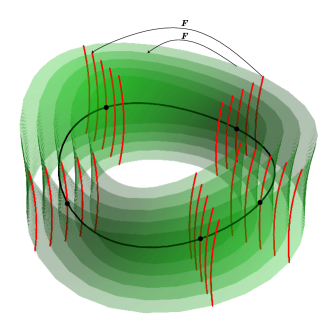
Within the context of this paper, an invariant foliation is a family of differentiable manifolds, called leaves, that fill up the phase space and are mapped onto each other by the map (1). To represent a foliation, we use an analytic function , where is an inner product vector space such that . The leaves of the foliation are parametrised by the elements of and given as level surfaces of the representing function in the form of
In our notation the foliation is the collection
| (20) |
Foliation is invariant if there exists a map , such that the invariance equation
| (21) |
holds. Equation (21) is the same as the inclusion . A schematic of a foliation about an invariant closed curve can be seen in figure 1.
Without losing generality, we assume that , which can be achieved by defining the and dropping the tilde from . To normalise the relation between and , we assume that and therefore . An invariant foliation is defined for a set of invariant vector bundles about the torus . The following theorem lays down the conditions when such foliation exists and unique.
Theorem 6.
Assume an invariant torus (2) and a linearised system about the torus in the form of (4). Also assume that the linear system has dichotomy spectral intervals given by (12) or (13) and that . Pick one or more spectral intervals using a non-empty index set
with the condition that for all so that linear the system (4) restricted to the subset of the spectrum
is invertible. Define the spectral quotient as
If the non-resonance conditions
| (22) |
hold for , such that there exists and then
-
1.
there exists a unique invariant foliation defined by analytic functions and satisfying equation (21) in a sufficiently small neighbourhood of the torus such that ;
-
2.
the nonlinear map is a polynomial, which in its simplest form contains terms for which the internal non-resonance conditions (22) with and does not hold.
Proof.
The proof has three steps. First we find a polynomial approximation of the invariant foliation which takes into account all possible resonance conditions. Second, we calculate an exact and unique correction to the polynomial expansion of the foliation. Finally, we establish that despite our choice of terms in the polynomial expansion, the calculated foliation is unique as a geometric object.
To make calculations simpler, we first shift the torus to the origin, such that the new map is and drop the hat from . This normalises our system such that . In addition, we choose , and then it follows from (21) that .
Continuing with our plan, we expand the two unknowns of the invariance equation (21) in the form of
| (23) | ||||
| (24) |
where is a polynomial order that will be clarified later. In the first step of the solution of (21), we solve for the polynomial coefficients and . In the second step, we solve for the correction term . In our case, the nonlinear map will remain a polynomial.
The linear terms , are recovered from the linearisation of the invariance equation (21) about the origin, which is
| (25) |
where . The matrices and can be found from the dichotomy spectral decomposition of matrix as per corollary 4. Noticing that the linearised invariance equation (25) is the same as (9), we find that
We solve for the nonlinear terms in increasing order, starting with . We can do this procedure, because terms of order only depend on unknown terms of order or lower. The equation for the order- terms is given by
| (26) |
where is composed of polynomial coefficients of and of order less than , and terms of . Equation (26) is linear for the polynomial coefficients and . Equation (26) can also be split up into independent lower dimensional equations on invariant subspaces, that are created from the invariant subspaces of . For the vector space , we need to introduce the decomposition such that , the identity is and , where is the Kronecker delta. We also decompose using in its range and in its domain. This further decomposition leads to the expressions
where the indices are and for and for . Substituting into (26) and multiplying from the left by and finally noting that we find that
| (27) | ||||
| (28) |
where
The only difference between (27) and (28) is the term , and therefore we treat the two equations together. For now, we set and solve for in both equations as long as it is possible.
To bring (28) into a more convenient form, we multiply (28) by from the left and find
| (29) |
Equation (29) is still in a cumbersome form, therefore we introduce the vectorisation and define operator and its inverse by
Equation (29) is now in a simpler form
| (30) |
which can be solved by finding the limit of either the forward iteration
| (31) |
or the inverse iteration
| (32) |
Expanding the iterations (31) and (32) yields
| (33) | ||||
| (34) |
First we find out the condition for convergence of (33) based on the exponential dichotomies of and that requires us to calculate the bounds on the term
| (35) |
Using the properties of tensor products and the exponential bounds (15) and (17) we find that
for , , where . For the inverse iteration we investigate the term
whose bound can be found in the same ways from equations (15) and (17) as
where , for . This means that either of the series converges to a unique analytic function if or . In summary, we can solve equation (29) if , which is called our non-resonance condition (22).
We now discuss the case of internal resonances, i.e., when (27) cannot be solved with , because for an index set . In this case we set and in (27), which is a solution of (27).
We note that no resonances are possible if either a) or b) . In case a) we must have
which implies the sub-cases
| (36) | ||||
In case b), we must have
which implies the sub-cases
| (37) |
Only sub-cases (36) and (37) make sense, because we want to have a lower bound on polynomial orders for which there are no resonances. We also note that (36) and (37) are identical if we replace (and therefore ) by its inverse. Therefore we only focus on the case when the invariant torus is an attractor, that is (37). We also notice that (37) is the same as stipulated in our theorem.
What remains is to find the correction term . We denote the truncated expansion by
and this way we can write the invariance equation (21) as
| (38) |
Applying the inverse to both sides of (38), yields
which translates to finding a root of the operator
| (39) |
To aid this endeavour, we introduce a new norm on the space of analytic functions
which defines the Banach space
We use theorem 7 to establish the existence of a unique root of . First we calculate the quantities
Due to the polynomial approximation of the actual solution by , for all there is a such that . We also notice that is Lipschitz continuous in the operator norm induced by and therefore the Lipschitz constant is finite. We now establish that
is invertible, where
Again, due to the polynomial approximation, is arbitrarily close to
for sufficiently small . Therefore if is a contraction, there is a such that is a contraction, too. We can only establish whether is a contraction after a number of iterations, and therefore we calculate
Calculating
| (40) |
takes a number of steps. Using (18) we estimate that
for . Given that for sufficiently large , we concluded that if
so is . This implies that the norm (40) is bounded by
Now all we need is that
and then for sufficiently large that . This the implies that is a contraction and so is for sufficiently small. This also means that and that is arbitrarily small. As a result we can apply theorem (7) and find that we have a unique solution for .
The last thing to show is uniqueness. In our calculation we have shown that for any permissible choice of , we have a unique . It is also clear that between two permissible and there is always a transformation , such that
| (41) |
because equation (41) has the exact same non-resonance conditions and choices for as the invariance equation (21). Now we notice that together with also satisfies the invariance equation (21) and that is the unique encoder, given . Therefore we conclude that any two solutions of (21) only differ by coordinate transformation . This makes the invariant foliation a unique geometric object. ∎
3 Numerical implementation
We use truncated Fourier series to represent functions along the torus , so that a function is given by
where are the values we hold in the computer memory. We also need to use the shift operator
which then implies that
and therefore the discretised shift operator is the diagonal matrix
Our map is given as a Fourier series , and therefore the invariant torus is a solution of
which are well-defined algebraic equations if the torus itself is normally hyperbolic.
3.1 Invariant vector bundles
To find the invariant vector bundles, we solve equation (9) in its discrete form and also with a constant and diagonal . A constant is only allowed due to discretisation, otherwise we would need to consider irreducibility. Diagonality of is also due to the numerical methods that ignore generalised eigenvectors. The discretised spectral equation is
| (42) |
where are the diagonal elements of . Equation (42) is an eigenvector-eigenvalue problem. We also consider the eigenvalue problem related to (10) in the form of
| (43) |
which has the same eigenvalues as (42).
The eigenvalues are placed approximately along concentric circles and we expect that each circle contains or eigenvalues, depending on whether they can be represented by a real or a pair of complex conjugate eigenvalues. Using k-nearest neighbours [4], we first try to find clusters for the magnitudes of the eigenvalues , expecting each cluster to have eigenvalues. If this does not hold, we decrease until each cluster has an integer multiple of eigenvalues while . It is possible to not find clusters that match our requirement, and there could be many reasons for that. For example, the value of , the number of Fourier harmonics could be too low, or the actual spectral circles are too close to each other to resolve them numerically. After a successful search we have clusters, denoted by such that .
We now need to identify a representative eigenvalue for each cluster of eigenvalues. We pick the one that corresponds to an eigenvector whose dominant Fourier component has the smallest index in magnitude. In mathematical formalism, if the eigenvectors are represented by , where is the index within the cluster we find the minimising index by
| (44) |
Using the identified eigenvectors , we recover the left and right invariant vector bundles of the linear system (4) in the form of
Finally, the coordinate transformation that brings the nonlinear system (1) into a form with diagonal and constant linear part is
and the transformed map about the invariant torus is obtained as
where .
3.2 Invariant foliation by series expansion
To create an invariant foliation we need to pick an index set that designates a set of diagonal elements of , which should include complex conjugate pairs if a complex eigenvalue is chosen. To make notation simpler, we assume that the first diagonal elements of are the chosen eigenvalues, as we are free to order them as necessary, thus . Using a mixed power and Fourier series expansion we then solve the invariance equation
| (45) |
The ansatz is a mixed trigonometric power series
where
and are the -th canonical unit vectors of the right dimension, e.g., . Substituting the ansatz into (45) and separating the -th order terms leads to the homological equation
| (46) |
where are terms composed of and , , .
We solve the homological equation (46) in increasing order of . The linear solution can be chosen as
The nonlinear terms are determined by equation
which has the solution
| (47) | ||||||
| (48) |
It is only possible to choose solution (47) if any of the indices are not part of . Therefore we must have
| (49) |
when any of the indices are not part of . This is the same condition as (22) expressed in a discretised fashion. If we have the denominator determines whether we choose solution (48) over (47).
In this paper we insist to create a independent, i.e, autonomous and therefore, we are only allowed to choose (48) for . This excludes parametric resonances, where (49) does not hold for .
Invariant manifolds can be calculated in the same way, except that the invariance equation is (52). We do not detail how this is done, because the invariant manifold can also be recovered from two complementary invariant foliations as described in the following section. The same holds true for invariant manifolds of vector fields, which are calculated by series expanding .
3.3 Reconstructing invariant manifolds
We assume that two foliations are calculated to satisfy the two invariance equations
| (50) | ||||
| (51) |
such that the sought after invariant manifolds is defined by with the dynamics represented by the map . To make sure that the two foliations are complementary, for equation (51) we use the index set . In order to find a manifold immersion such that the manifold invariance equation
| (52) |
holds we need to solve the equations
| (53) |
We assume that the encoders are separated into linear and nonlinear parts, such that and . The equations (53) can be re-written into the following form
and can be solved by iteration
| (54) |
3.4 Frequencies and damping ratios
As we have discussed previously [24], the dynamics given by the map should be interpreted in the nonlinear coordinate system given by the manifold immersion . This means that the dynamical properties cannot just be derived from map , the immersion also needs to be considered. Here we summarised how this is done, and refer to the companion paper [25], for detailed derivation. Here we are concerned about the frequencies and damping ratios of the vibration that surrounds the invariant torus and contained within the invariant manifolds . Therefore we assume that is autonomous as per the transformation in section 3.2, but remains -dependent. It is also assumed that the manifold is two-dimensional for each point of the torus and the linear part if has a pair of complex conjugate eigenvalues. Under these assumptions we can write that
| (55) |
where function is scalar valued, and means complex conjugation. Given the form (55), we can use a polar coordinate system and therefore define
such that the invariance equation (45) becomes
We now need to create a transformation that makes sure two things: the amplitude given by increases linearly with parameter and that there is no phase shift between closed curves defined by the graphs of and for . The first condition makes sure that damping ratios are correct, the second makes sure that frequencies are correct. A lengthy derivation in [24] yields that this transformation is
where
with
In the new corrected coordinate system the invariance equation becomes
where
Given that we no longer have amplitude and phase distortion, the instantaneous frequency and the damping ratio can be calculated as
respectively, where is the duration of time, between two consecutive points of the trajectory generated by . The ROM in differential equation form becomes
4 Examples
Here we investigate two examples, which are both two degree-of-freedom mechanical systems. Due to limitations of polynomial expansions, we will not consider higher dimensional systems here, those can be found in the companion paper [25], where a more suitable representation of the submersions and is used. The calculations have the following steps
-
1.
Calculate a discrete-time map from the vector field (ODE) by Taylor expanding a numerical ODE solver using automatic differentiation.
-
2.
Identify the invariant torus (periodic orbit) from both the ODE and the generated map. (not detailed here)
-
3.
Identify invariant vector bundles about the torus (ODE and map) as in section 3.1.
-
4.
Calculate the sought after invariant manifold directly (ODE and map). (not detailed here)
- 5.
-
6.
Recover the frequencies and damping ratios for the sought after vibration mode (section 3.4) for all models and manifolds identified.
When comparing various methods for calculating the ROM, we use the relative error
| (56) |
as a measure of accuracy. We also consider how the error depends on the amplitude, that is calculated as .
4.1 A planar oscillator
The first example is a forced geometrically nonlinear oscillator. This oscillator appeared in [26] without forcing and damping. The schematic of the oscillator can be seen in figure 2.
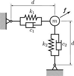
The equations of motion are
| (57) |
The unforced natural frequencies are , , the spectral quotients and . When forcing with amplitude and frequency , the natural frequencies become , and the spectral quotients become , .
The spectrum, the invariant torus, the invariant manifold and information about the vector bundle are depicted in figure 3. The spectrum points in figure 3(b) are calculated as , where is the spectrum point of the discrete-time dynamics (see section 3.1) and is the sampling period. The four spectrum points that are used to calculate the vector bundles are denoted by stars and a triangle.
We calculate the ROM in three different ways. First we solve the invariance equation for the ordinary differential equation, which is
| (58) |
secondly we solve the invariance equation (52) for the generated Poincare map and finally we use invariant foliations to obtain the ROM. The result of our calculation can be seen in figure 2.
We notice that different calculations only agree for lower amplitudes, we notice that the disagreement starts to occur when the mean relative error increases above . The error of different calculations of the same ROM are very close, which cannot explain the different results. The most likely explanation is that the radius of convergence of the power series expansion is at lower amplitudes than the maximum displayed in figure 4. Fitting the invariance equations to data can overcome the problem with the radius of convergence. We also note that it was necessary to use order Fourier collocation to reduce the calculation error at zero amplitudes. Order has provided a uniform error just below for all amplitudes (data not shown).
4.2 Two-mass oscillator with nonlinear springs and dampers
As opposed to the geometrically nonlinear system, we consider a system that is geometrically linear but has nonlinear components. The system, as shown in figure 5, consists of two block masses sliding on a frictionless surface. The two masses are connected by nonlinear springs and linear dampers. Forcing is applied to both masses with a phase shift.
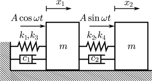
The equations of motion are
| (59) |
The unforced natural frequencies are and with damping ratios and . The spectral quotients are and . With forcing at the natural frequencies are , with damping ratios and . With forcing, the spectral quotients become and .
The results can be seen in figure 7. When calculating the ROMs, we notice that we can achieve better accuracy than in the previous example of section 4.1. The instantaneous frequencies agree well, but there are differences for the forced system at higher amplitude, which again could be due to the radius of convergence of the asymptotic power series expansion. The instantaneous damping shows greater differences. In general, we find that instantaneous damping ratios are sensitive to how they are calculated numerically.
As a final calculation, we demonstrate that even if we only calculate the conjugate map up to linear order, we can still recover nonlinear behaviour that is encoded within the coordinate system represented by the invariant foliations and manifolds. In figure 8 we calculated the invariant manifolds of the vector field (59) to order 7, while the conjugate map remained linear when the invariant manifold and the invariant foliations were calculated. Figure 8 shows that while the relative accuracy of the calculation reduces with assuming a linear , for small amplitudes we can reconstruct frequencies and damping rations accurately. For higher amplitudes the instantaneous frequency and damping curves diverge earlier than in figure 7.
5 Conclusions
We have shown the existence and uniqueness of invariant foliations about quasi-periodic tori. The results are similar to the autonomous case detailed in [23], but they are more restrictive, because the non-resonance conditions involve not only individual spectral points, but concentric circles. In practice, however, the resonance conditions will remain discrete, even though the discretised transfer operator still has many more spectral points than in the autonomous case. In this paper we have eliminated all non-autonomous resonances and therefore the normal form of the ROM became autonomous. This allowed us to depict the vibrations about the invariant torus with frequencies and damping ratios independent of where they are along the torus. In situations where the forcing has resonances with the underlying system, this is not possible.
The accuracy of the calculations was also investigated, showcasing the differences between various methods of calculating ROMs. We conjecture that the differences are due to the asymptotic nature of the calculations, which has a radius of convergence that is smaller than the range of amplitudes the we might be interested in.
In the companion paper [25], we investigate how fitting invariant foliations directly to data affects accuracy. We will also highlight that in a data-driven setting the smoothness criterion of theorem 6 for uniqueness is unhelpful, because the data fitting is global as opposed to asymptotic about the invariant torus. Therefore our ongoing work focusses on finding better uniqueness criteria that better aligns with data-driven methods.
Appendix A Newton-Kantorovich theorem
The main tool that we use for establishing the existence and uniqueness of the invariant torus and the invariant foliation is the Newton-Kantorovich theorem. The theorem is useful as it replaces contraction mapping arguments used elsewhere.
Theorem 7.
Let and be Banach spaces and consider an open subset of , a point and a map such that both . Assume three constants such that
Then the sequence is contained in the ball where
and converges to the unique zero of in .
Appendix B Existence and uniqueness of the invariant torus
An invariant foliation is always specific to an underlying invariant object, which in our case is an invariant torus. The torus can be represented as a graph over the space which we denote by
The existence of a unique invariant torus can only be guaranteed locally near an approximate solution of the invariance equation (3). The condition besides having a good approximation is that the approximate solution is hyperbolic. The following result is well-know, for example from [16, 15].
Theorem 8.
Assume that such that and that , where . Then for a sufficiently small , equation (3) has a unique solution for in in a small neighbourhood of .
Proof.
Since this has been detailed in [16], we just provide a sketch of the proof. Define the operator as
| (60) |
The Frechet derivative of operator at the origin is
Now we refer to theorem 7 to show that (60) has a unique solution. By our assumption , is invertible due to corollary 3, hence is finite. Since is linearly increasing with the Lipschitz constant is also finite. In addition we can make as small as necessary because is sufficiently small due to being a good approximation. Finally , which implies that as with a linear rate. Therefore, if is sufficiently small, we can achieve , which implies a unique solution to (60). ∎
Software
The computer code that produced the results in this paper can be found at https://github.com/rs1909/InvariantModels
References
- [1] Bernd Aulbach and Nguyen Van Minh. The concept of spectral dichotomy for linear difference equations ii. Journal of Difference Equations and Applications, 2(3):251–262, 1996.
- [2] Bernd Aulbach and Thomas Wanner. Invariant foliations and decoupling of non-autonomous difference equations. Journal of Difference Equations and Applications, 9(5):459–472, 2003.
- [3] P. W. Bates, K. Lu, and C. Zeng. Invariant foliations near normally hyperbolic invariant manifolds for semiflows. Trans. Amer. Math. Soc., 352(10):4641–4676, 2000.
- [4] G. Biau and L. Devroye. Lectures on the Nearest Neighbor Method. Springer Series in the Data Sciences. Springer, 2015.
- [5] X. Cabré, E. Fontich, and R. de la Llave. The parameterization method for invariant manifolds I: Manifolds associated to non-resonant subspaces. Indiana Univ. Math. J., 52:283–328, 2003.
- [6] X. Cabré, E. Fontich, and R. de la Llave. The parameterization method for invariant manifolds iii: overview and applications. Journal of Differential Equations, 218(2):444–515, 2005.
- [7] Philippe G. Ciarlet and Cristinel Mardare. On the Newton-Kantorovich theorem. Analysis and Applications, 10(3):249 – 269, 2012.
- [8] Matthew J. Colbrook and Alex Townsend. Rigorous data-driven computation of spectral properties of koopman operators for dynamical systems. Communications on Pure and Applied Mathematics, 2023.
- [9] R. de la Llave. Invariant manifolds associated to nonresonant spectral subspaces. Journal of Statistical Physics, 87(1):211–249, 1997.
- [10] R. de la Llave and C. E. Wayne. On irwin’s proof of the pseudostable manifold theorem. Mathematische Zeitschrift, 219:301–321, 1995.
- [11] N. Fenichel. Persistence and smoothness of invariant manifolds for flows. Indiana Univ. Math. J., 21:193–226, 1972.
- [12] José Antonio Ezquerro Fernández and Miguel Ángel Hernández Verón. Mild differentiability conditions for newton’s method in banach spaces. Frontiers in Mathematics, pages 1 – 178, 2020.
- [13] Celso Grebogi, Edward Ott, Steven Pelikan, and James A. Yorke. Strange attractors that are not chaotic. Physica D: Nonlinear Phenomena, 13(1):261–268, 1984.
- [14] G. Haller and S. Ponsioen. Nonlinear normal modes and spectral submanifolds: existence, uniqueness and use in model reduction. Nonlinear Dynamics, 86(3):1493–1534, 2016.
- [15] À. Haro, M. Canadell, Al. Luque, J. M. Mondelo, and J.-L. Figueras. The Parameterization Method for Invariant Manifolds: From Rigorous Results to Effective Computations, volume 195 of Applied Mathematical Sciences. Springer, 2016.
- [16] A. Haro and R. de la Llave. A parameterization method for the computation of invariant tori and their whiskers in quasi-periodic maps: Rigorous results. Journal of Differential Equations, 228(2):530–579, 2006.
- [17] M. W. Hirsch, C. C. Pugh, and M. Shub. Invariant manifolds. Bull. Amer. Math. Soc., 76(5):1015–1019, 09 1970.
- [18] R. Mañé. Persistent manifolds are normally hyperbolic. Transactions of the American Mathematical Society, 246:261–283, 1978.
- [19] A. Mauroy, I. Mezić, and J. Moehlis. Isostables, isochrons, and koopman spectrum for the action–angle representation of stable fixed point dynamics. Physica D: Nonlinear Phenomena, 261:19–30, 2013.
- [20] I. Mezić. Spectral properties of dynamical systems, model reduction and decompositions. Nonlinear Dynamics, 41(1-3):309–325, 2005.
- [21] J.J. Palis and W. de Melo. Geometric Theory of Dynamical Systems: An Introduction. Springer New York, 2012.
- [22] Robert J Sacker and George R Sell. A spectral theory for linear differential systems. Journal of Differential Equations, 27(3):320–358, 1978.
- [23] R. Szalai. Invariant spectral foliations with applications to model order reduction and synthesis. Nonlinear Dynamics, 101(4):2645–2669, 2020.
- [24] R. Szalai. Data-driven reduced order models using invariant foliations, manifolds and autoencoders. Journal of Nonlinear Science, 33(5):75, 2023.
- [25] R. Szalai. Machine-learning invariant foliations in forced systems for reduced order modelling, 2024.
- [26] C. Touzé, O. Thomas, and A. Chaigne. Hardening/softening behaviour in non-linear oscillations of structural systems using non-linear normal modes. Journal of Sound and Vibration, 273(1):77–101, 2004.
- [27] A. Vizzaccaro, Y. Shen, L. Salles, J. Blahoš, and C. Touzé. Direct computation of nonlinear mapping via normal form for reduced-order models of finite element nonlinear structures. Computer Methods in Applied Mechanics and Engineering, 384:113957, 2021.
- [28] S. Wiggins. Introduction to Applied Nonlinear Dynamical Systems and Chaos. Texts in Applied Mathematics. Springer New York, 2003.
- [29] S. Wiggins, G. Haller, and I. Mezic. Normally Hyperbolic Invariant Manifolds in Dynamical Systems. Applied Mathematical Sciences. Springer New York, 2013.