1 Introduction

The ATLAS experiment at the Large Hadron Collider confirms that proton-proton ($pp$) collisions at energy $\sqrt{s}\approx 13\,{\rm TeV}$ produce $t\bar{t}$ pairs of top quarks with an entangled spin structure as predicted by the Standard Model [1]. The Standard Model predicts that the dominant top pair production process at the LHC is from gluons, $gg\to t\bar{t}$. Since gluons have spin 1, two gluons produce maximally entangled top pairs in the spin-singlet state, $|t_{\uparrow}\bar{t}_{\downarrow}\rangle-|t_{\downarrow}\bar{t}_{\uparrow}\rangle$, around the kinematical threshold where tops are non-relativistic [2, 3]. The CMS experiment, which did not focus on non-relativistic top quarks, was unable to observe top quark entanglement [4]. Measuring top quark spins necessitates a sophisticated experimental analysis, as top quark spin is indirectly inferred from the angular distributions of the leptons resulting from weak top quark decays $t\to b\ell\bar{\nu}$, see fig. 1.

From a theoretical perspective this experimental result comes as no surprise. Indeed entanglement is a well known phenomenon [5, 6] at the basis of quantum mechanics that is currently receiving renewed attention. On one hand, the emergence of novel physics that alters entanglement seems implausible as any modification to quantum mechanics risks spoiling the quantum consistency of the Standard Model and, consequently, various observed quantities influenced by top-quark loops. On the other hand, conventional new physics scenarios (e.g., in the form of effective operators such as a chromo-magnetic dipole of the top [7, 8, 9, 3]) could easily impact entanglement by modifying the $gg\to t\bar{t}$ and/or $t\to b\ell\bar{\nu}$ processes. However, such modifications would also influence the rates summed over spins, which have been tested in multiple ways more extensively and more directly than entanglement itself. For example, modifying QCD would also affect the $gg\to t\bar{t}$ total cross section, and its angular and energy distributions summed over spins. So the following issues arise:

1. Do collider measurements of entanglement at high energy test any new physics theory? In section 2 we answer positively, proposing an unusual kind of new physics that does not affect differential rates summed over spins by a single bit, while affecting the qubit: spins and their entanglement get modified. In section 3 we show that this new physics can modify the top spin entanglement observable measured by ATLAS. This allows us to move beyond tree-level observables and address the next big issue:

2. Is new physics that affects top quark spin entanglement allowed by constraints on processes mediated by virtual top quarks at loop level, as observed in Higgs physics, electro-weak physics, flavour physics, low-energy physics?

This issue is addressed in section 4, and is particularly important because the new theoretical ingredient we introduced involves a non-local breaking of Lorentz invariance. Different unbroken Lorentz sub-groups are explored, and the maximal SIM(2) sub-group alleviates most unwanted loop effects. Conclusions and a summary of results are provided in section 5.

2 A theory for new physics in spin entanglement

We propose a modification of the usual relativistic Quantum Field Theory that, at tree level, leaves unaffected differential cross sections summed over spins, while modifying spins and thereby their entanglement. Our theory can be defined as follows: we replace a Dirac spinor field $\Psi(x)$ (for example the field describing top quarks) with

$$\tilde{\Psi}(x)=W(i\partial)\Psi(x)=\int\frac{d^{3}p}{(2\pi)^{3}}\frac{1}{\sqrt{2E_{p}}}\sum_{s}\left(\tilde{u}_{s}(p)a_{s\bm{p}}e^{-ip\cdot x}+\tilde{v}_{s}(p)b_{s\bm{p}}^{\dagger}\,e^{ip\cdot x}\right)$$ (1)

that differs from the standard expression because spinors are replaced by tilted ones

$$\tilde{u}_{s}(p)\equiv W(p)u_{s}(p),\qquad\tilde{v}_{s}(p)\equiv W(-p)v_{s}(p)$$ (2)

where $W(p)$ is a $4\times 4$ matrix in spinor space that introduces a relative orientation between spin in space-time and in spinor space, and $E_{p}^{2}=\mbox{\boldmath$p^{2}$}+M^{2}$. Different choices of $W(p)$ give different theories. If performed everywhere in the action, the

$$\Psi\to\tilde{\Psi}=W\Psi$$ (3)

replacement is a field redefinition that leaves physics invariant. The transformation introduces new physics if performed differently in different terms (for example, if performed in a sub-set of terms).

• We perform the $\Psi\to\tilde{\Psi}$ transformation of eq. (3) in the Dirac kinetic term of $\Psi$, that, in general, becomes a new operator $\tilde{\cal K}\neq{\cal K}\equiv\not{p}-M$:

  $${\bar{\Psi}}{\cal K}\Psi\to{\bar{\Psi}}\overline{W}(\not{p}-M)W\Psi\equiv{\bar{\Psi}}\tilde{\cal K}\Psi$$ (4)

  where $\overline{W}=\gamma_{0}W^{\dagger}\gamma_{0}$. The fermion propagator $\Pi(p)=i/(\not{p}-M)$ gets modified into

  $$\tilde{\Pi}(p)={W}^{-1}(p)\cdot\Pi(p)\cdot\overline{W}^{-1}(p).$$ (5)

  We will assume $W(p)$ has a non-local form such that

  $$\overline{W}W=\mathbb{1},\qquad\overline{W}\not{p}W=\not{p}$$ (6)

  because, as discussed later, this guarantees that spin-summed tree-level cross sections remain invariant. Then $\tilde{\cal K}$ and its inverse, the propagator $\tilde{\Pi}$, keep the usual Dirac form.

• Vertices that involve $\Psi$ get modified by extra $W$ matrices. For example, if $\Psi$ is the top quark field, we can assume that $\tilde{\Psi}$ transforms in the standard way under local QCD gauge invariance. Then the top/gluon interaction $g_{3}g^{a}_{\mu}(q_{g})T^{a}_{ij}\bar{\tilde{t}}_{i}(q_{1})\tilde{t}_{j}(q_{2})$ with $q_{1}+q_{2}+q_{g}=0$ gives the modified $g\bar{t}t$ vertex:
  gtt

  $$\begin{gathered}\fmfgraph*(22,14)\fmfleft{i}\fmfright{b,a}\fmflabel{$g_\mu,a$}{i}\fmflabel{$t,i$}{a}\fmflabel{$\bar{t},j$}{b}\fmf{gluon}{i,v1}\fmf{plain_{a}rrow}{v1,a}\fmf{plain_{a}rrow}{b,v1}\fmfdot{v1}\fmfcmd{style_{d}efmarrowdexprp=drawarrowsubpath(1/3,3/4)ofpshifted12upwithpenpencirclescaled0.5;label.top(btex$q_1$etex,point0.5ofpshifted18up);enddef;}\fmf{marrowd,tension=0}{v1,a}\fmfcmd{style_{d}efmarroweexprp=drawarrowsubpath(1/3,3/4)ofpshifted12downwithpenpencirclescaled0.5;label.bot(btex$q_2$etex,point0.5ofpshifted18down);enddef;}\fmf{marrowe,tension=0}{v1,b}\end{gathered}\quad=~{}~{}-ig_{3}T^{a}_{ij}\,\overline{W}(q_{1})\gamma^{\mu}W(-q_{2}).$$ (7)

Amplitudes will remain unmodified because, in Feynman diagrams, the inverse $W(p)$ factors arising from propagators in eq. (5) cancel with the $W(p)$ factors arising from vertices. Next, the extra cancellation of $W(p)$ factors within propagators will ensure that spin-summed cross sections remain unmodified. On the other hand, spins get rotated by $W(p)$ provided that rotational invariance and thereby Lorentz invariance is broken by $W(p)$. We recall that a Lorentz transformation $S\stackrel{{\scriptstyle\Lambda}}{{\to}}S^{\prime}$ from a reference frame $S$ to a frame $S^{\prime}$ acts on coordinates as $x^{\prime}=\Lambda x$ and in Hilbert space as the operator ${\cal U}_{\Lambda}$

$${\cal U}_{\Lambda}a_{s\bm{p}}{\cal U}^{-1}_{\Lambda}=\sqrt{\frac{E_{p^{\prime}}}{E_{p}}}\,D_{ss^{\prime}}^{-1}(\Lambda,p)\,a_{s^{\prime}\bm{p}^{\prime}},\qquad p^{\prime}=\Lambda p$$ (8)

where $D$ is the unitary spin-representation of the Wigner spatial rotation associated to $\Lambda$ and $p$. So the field $\tilde{\Psi}$ Lorentz transforms into

$${\cal U}_{\Lambda}\tilde{\Psi}(x){\cal U}^{-1}_{\Lambda}=\Lambda_{1/2}^{-1}\int\frac{d^{3}p^{\prime}}{(2\pi)^{3}}\frac{1}{\sqrt{2E_{p^{\prime}}}}\sum_{s^{\prime}}\left[W^{\prime}(p^{\prime})a_{s^{\prime}\bm{p}^{\prime}}u_{s^{\prime}}(p^{\prime})e^{-ip^{\prime}\cdot x^{\prime}}+W^{\prime}(-p^{\prime})b_{s^{\prime}\bm{p}^{\prime}}^{\dagger}v_{s^{\prime}}(p^{\prime})e^{ip^{\prime}\cdot x^{\prime}}\right]$$ (9)

showing that, in addition to the usual $\Lambda_{1/2}$ Lorentz matrix acting on spinors, the extra factor $W(p)$ transforms into

$$W(p)\stackrel{{\scriptstyle\Lambda}}{{\to}}W^{\prime}(p^{\prime})=\Lambda_{1/2}W(p=\Lambda^{-1}p^{\prime})\Lambda_{1/2}^{-1}\,.$$ (10)

Different forms of $W(p)$ break the Lorentz group down to different sub-groups $H$. Furthermore, the space-time discrete symmetries parity P, charge conjugation C, and time reversal T transform $W(p)$ as

$$\begin{array}[]{rcl}W(p)\xrightarrow{\rm P}&W^{\prime}({\rm P}\,p)&=\gamma^{0}W(p)\gamma^{0}\,,\cr W(p)\xrightarrow{\rm C}&W^{\prime}(-p)&=C{W}^{\ast}(p)C\cr W(p)\xrightarrow{\rm T}&\!\!W^{\prime}({\rm P}\,p)\!\!&=\gamma^{3}\gamma^{1}W^{\ast}(p)\gamma^{1}\gamma^{3}\end{array}$$ (11)

where ${\rm P}\,(p_{0},\mbox{\boldmath$p$})=(p_{0},-\mbox{\boldmath$p$})$ and $C=-i\gamma^{2}$. In the next 3 sections we will consider three possible symmetry breaking patterns:

1. In section 2.1 we naively break Lorentz to SO(2,1).

2. In section 2.2 we try breaking rotational invariance while keeping the associated breaking of boosts as mild as possible.

3. In section 2.3 we break Lorentz down to its phenomenologically acceptable maximal sub-group $H={\rm SIM}(2)$ that contains all boosts (combined with rotations), such that a special orientation is introduced without that any rest frame becomes special.

2.1 Lorentz broken to SO(2,1)

The Lorentz group contains 3 rotation generators $J_{x,y,z}$ and 3 boost generators $K_{x,y,z}$. As a first naive attempt we break Lorentz to the sub-group $H$ that leaves invariant the space-like unit vector

$$n^{\mu}=(0,\mbox{\boldmath$n$})=(0,0,0,1).$$ (12)

Without loss of generality we can orient the $z$ axis along $n$, so that $H=\,{\rm SO}(2,1)$ is spanned by the three $J_{z},K_{x},K_{y}$ generators. We assume the following two forms of $W(p)$:

1. Two equal rotations with angle $\delta/2$ around the $n$ axis:

   $$W(p)=\exp\left(i\delta\frac{[\not{n},\not{p}]\gamma_{5}}{8M_{p}}\right),\qquad W(0)=\,{\rm diag}(e^{i\delta/4},e^{-i\delta/4},e^{i\delta/4},e^{-i\delta/4}).$$ (13)

   We define $M_{p}^{2}\equiv p\cdot p$ as $M_{p}\geq 0$ if $p^{0}>0$ and as $M_{p}\leq 0$ if $p^{0}<0$, such that $W(p)=W(-p)$ and a common $W$, denoted as $W(0)$, rotates in the same way spins of particles and anti-particles produced at rest. This $W(p)$ is invariant under C, P and T, see table 1. The opposite choice would give opposite rotations, more simply obtained in the second example below.

2. Two opposite rotations with angle $\delta/2$ around the $n$ axis:

   $$W(p)=\exp(-i\delta\,\not{n}\gamma_{5}/4),\qquad W(0)=\,{\rm diag}(e^{i\delta/4},e^{-i\delta/4},e^{-i\delta/4},e^{i\delta/4}).$$ (14)

   This $p$-independent $W$ respects P and T but breaks C, because particles and anti-particles couple in opposite way to breaking of rotational invariance.

In view of their exponential form, both $W(p)$ satisfy eq. (6) and consequently leave unaffected the spin-summed tree-level cross sections. Both $W(p)$ rotate spins, and thereby affect spin entanglement. However, at loop level, these theories are subject to strong bounds on Lorentz breaking. In the next two sections we thereby consider less problematic forms of Lorentz breaking.

Lorentz broken to	Theory with $W(p)$ given by	P	T	C	PT	CP	CT	CPT
SO(2,1)	eq. (13), same rotation	$+$	$+$	$+$	$+$	$+$	$+$	$+$
SO(2,1)	eq. (14), opposite rotation	$+$	$+$	$-$	$+$	$-$	$-$	$-$
SO(2)	eq. (22), same rotation	$+$	$+$	$+$	$+$	$+$	$+$	$+$
SO(2)	eq. (23), opposite rotation	$+$	$+$	$-$	$+$	$-$	$-$	$-$
SIM(2)	eq. (27), boost	$\color[rgb]{0.45,0,0}\times$	$\color[rgb]{0.45,0,0}\times$	$+$	$+$	$\color[rgb]{0.45,0,0}\times$	$\color[rgb]{0.45,0,0}\times$	$+$
SIM(2)	eq. (28), same rotation	$\color[rgb]{0.45,0,0}\times$	$\color[rgb]{0.45,0,0}\times$	$+$	$+$	$\color[rgb]{0.45,0,0}\times$	$\color[rgb]{0.45,0,0}\times$	$+$
SIM(2)	eq. (29), opposite rotation	$\color[rgb]{0.45,0,0}\times$	$\color[rgb]{0.45,0,0}\times$	$-$	$+$	$\color[rgb]{0.45,0,0}\times$	$\color[rgb]{0.45,0,0}\times$	$-$

Table 1: Transformation properties of the various $W(p,\delta)$ under space-time discrete symmetries S. A $\color[rgb]{0.45,0,0}\times$ means that the symmetry is broken. A $+$ means that $W(p,\delta)\xrightarrow{\rm S}W({\rm S}\,p,\delta)$ is invariant. A $-$ means that $W(p,\delta)\xrightarrow{\rm S}W({\rm S}\,p,-\delta)=W({\rm S}\,p,\delta)^{-1}$, namely that $\delta$ is odd under S.

2.2 Lorentz broken to SO(2)

We modify the theory of section 2.1 by trying to make the unavoidable breaking of boosts as mild as possible. We start by considering a $\Psi$ particle at rest (denoted as 0) in the reference frame $S$. We assume that, in the Dirac basis,

$$W(0)=\,{\rm diag}(U,\epsilon V^{*}\epsilon^{-1})$$ (15)

where $\epsilon$ is the $2\times 2$ anti-symmetric tensor and $U,V$ are two $2\times 2$ matrices. The spinor polarizations can be written in terms of their values at rest as $u(p)=\Lambda_{p}u(0)$ and $v(p)=\Lambda_{p}v(0)$, where

$$\Lambda_{p}=\frac{M_{p}+\not{p}\gamma^{0}}{\sqrt{2M_{p}(p_{0}+M_{p})}}.$$ (16)

is the Lorentz transformation that brings to rest a time-like vector $p_{\mu}$, $\Lambda^{-1}_{p}\not{p}\Lambda_{p}=p\gamma_{0}$, with $M_{p}$ defined below eq. (13). Trying to preserve Lorentz invariance as much as possible we demand $\tilde{u}(p)=\Lambda_{p}\tilde{u}(0)$ and $\tilde{v}(p)=\Lambda_{p}\tilde{v}(0)$, obtaining

$$W(p)=\Lambda_{p}W(0)\Lambda_{p}^{-1}.$$ (17)

Since $W(0)$ commutes with $\gamma_{0}$, the condition in eq. (6) for preserving the total cross sections is satisfied if $U,V$ are U(2) rotations:

$$U^{\dagger}U=\mathbb{1}=V^{\dagger}V.$$ (18)

Later computations will be simplified by noticing that this new physics can be equivalently rewritten as the constant matrices $U,V$ acting on the spin indices

$$\tilde{u}_{s}(p)\equiv u_{s^{\prime}}(p)U_{s^{\prime}s},\qquad\tilde{v}_{s}(p)\equiv v_{s^{\prime}}(p)V_{s^{\prime}s}^{*}.$$ (19)

Then the general Lorentz transformation of eq. (10) reduces to

$$U\to U^{\prime}=DUD^{-1},\qquad V\to V^{\prime}=DVD^{-1}$$ (20)

showing that $U$ and $V$ transform as rotations. This means that $U,V\neq\mathbb{1}$ break rotational invariance and that Lorentz invariance is broken too, but only by the Wigner rotations $D$ associated to boosts. Boosts are broken in the following mild way: the reference frame $S$ is special because in $S$ the breaking of rotational invariance has the simple form of eq. (17).

Eq. (11) implies that parity P, charge conjugation C, and time reversal T act on $U,V$ as

$$\begin{array}[]{llll}\hbox{P:}&U\xrightarrow{\rm P}U&V\xrightarrow{\rm P}V\cr\hbox{C:}&U\xrightarrow{\rm C}V&V\xrightarrow{\rm C}U\cr\hbox{T:}&U\xrightarrow{\rm T}\epsilon U^{*}\epsilon^{-1}&V\xrightarrow{\rm T}\epsilon V^{*}\epsilon^{-1}\end{array}$$ (21)

Notice that $\epsilon U^{*}\epsilon^{-1}=U$ if $U$ is a $\,{\rm SU}(2)$ rotation, and similarly for $V$. In the following we will assume that $U$ and $V$ are SU(2) rotations, so that T is conserved and $W=\,{\rm diag}(U,V)$. In order to break Lorentz invariance minimally we will consider two sub-cases, C-even and C-odd, analogous to the ones in section 2.1:

1. $V=U$ are two equal rotations with angle $\delta/2$ around the same axis $n$. Then $W(0)$ is a rotation in 4-dimensional spinor space, and conserves C, as well as P and T. A rotation remains $W(0)=\,{\rm diag}(U,U)$ also in the Weyl basis. It can be written as

   $$W(p)=\exp(i\delta\,[\not{n}_{p},\not{p}]\gamma_{5}/8M_{p})$$ (22)

   which is a rotation with angle $\delta/2$ around the boosted $n^{\mu}_{p}=(\Lambda_{p})^{\mu}_{~{}\nu}n^{\nu}$. For $p$ at rest and $n$ along the $z$ axis it reduces to $W(0)=\,{\rm diag}(e^{i\delta/4},e^{-i\delta/4},e^{i\delta/4},e^{-i\delta/4})$ as in eq. (13), having defined $M_{p}$ in the same way.

2. $V=U^{-1}$ are two opposite rotations with angle $\delta/2$ around the same axis $n$. The assumed $W=\,{\rm diag}(U,U^{-1})$ in the Dirac basis can be written in a basis-independent way as

   $$W(p)=\exp(-i\delta\,\not{n}_{p}\gamma_{5}/4).$$ (23)

   For $p$ at rest and $n_{p}=n$ along the $z$ axis it reduces to $W(0)=\,{\rm diag}(e^{i\delta/4},e^{-i\delta/4},e^{-i\delta/4},e^{i\delta/4})$ as in eq. (14). The parameter $\delta$ is odd under C, because particles and anti-particles couple in opposite way to breaking of rotational invariance. P and T are conserved, so $\delta$ is odd also under CP and CPT (see table 1).

These $W(p)$ differ from the analogous one in eq.s (13) and  (14) because $n$ has been promoted into $n_{p}$. As a result all boosts are broken, but only by the Wigner matrices that rotate $n^{\mu}$. The Lorentz group is broken to SO(2), describing rotations around $n$.

2.3 Lorentz broken to its maximal sub-group SIM(2)

The maximal Lorentz sub-group $H={\rm SIM}(2)$ is spanned by the 4 generators [10, 11]

$$J_{z},\qquad K_{z},\qquad T_{1}=K_{x}+J_{y},\qquad T_{2}=K_{y}-J_{x}.$$ (24)

The light-cone combinations $T_{1}$ and $T_{2}$ commute, forming a group of 2-dimensional translations. The SIM(2) sub-algebra closes as

$$[T_{1},K_{z}]=iT_{1},\qquad[T_{2},K_{z}]=iT_{2},\qquad[T_{1},J_{z}]=-iT_{2},\qquad[T_{2},J_{z}]=iT_{1}.$$ (25)

$H$ is denoted as SIM(2) because this Lie algebra is equivalent to the one of similitude transformations in 2 dimensions. SIM(2) contains all boosts $K_{x,y,z}$, so a generic time-like 4-vector can be rotated to its rest frame (at the price of an extra Wigner rotation performed by $K_{x,y}$ in $T_{1,2}$) and the speed of light $c$ remains universal [11, 12]. The vector

$$n^{\mu}=(1,0,0,1)$$ (26)

is invariant under the sub-group spanned by $T_{1},T_{2},J_{z}$ and transforms multiplicatively under $K_{z}$. Thereby Lorentz-breaking SIM(2)-invariant theories can be written from non-local ratios of terms containing the same power of $n$ [11]. This can be immediately generalized to $n^{\mu}=(1,\mbox{\boldmath$n$})$. Notice that $n^{\mu}$ differs from the previous sections 2.1 and 2.2, where $n^{\mu}=(0,0,0,1)$ resulted in different sub-groups. We present three concrete SIM(2)-invariant theories, corresponding to 3 choices of $W(p)$.

1. Assuming that $W$ is a boost along $n$ with parameter $\delta$ gives

   $$W(p)=\exp\left(\frac{\delta}{4}\frac{[\not{n},\not{p}]}{n\cdot p}\right),\qquad\tilde{\cal K}\equiv\overline{W}(\not{p}-M)W=e^{\delta}\not{p}-M-\frac{p^{2}\,\not{n}}{p\cdot n}\sinh\delta.$$ (27)

   This analytic $W(p)$ satisfies $\overline{W}W=1$, so $\tilde{{\cal K}}^{2}=p^{2}-M^{2}$ reproducing the standard relativistic dispersion relation. The modified Dirac operator $\tilde{\cal K}$ generalises the theory proposed in [13] for $M=0$. Since $\tilde{\cal K}\neq{\cal K}$ this theory affects spin-summed cross sections.

2. A different SIM(2)-invariant theory is obtained assuming that $W(p)$ is a rotation with angle $\delta/2$ around $n$ acting in the same way on particles and anti-particles (analogously to the C-even cases 1. in sections 2.1, 2.2):

   $$W(p)=\exp\left(i\frac{\delta}{4}\frac{[\not{n},\not{p}]\gamma_{5}}{n\cdot p}\right),\qquad W(0)=\,{\rm diag}(e^{i\delta/4},e^{-i\delta/4},e^{i\delta/4},e^{-i\delta/4}).$$ (28)

   This analytic $W(p)$ satisfies eq. (6) leaving the Dirac operator unchanged, $\tilde{\cal K}={\cal K}$, and leaving spin-summed tree cross sections unchanged.

3. One more SIM(2)-invariant theory is obtained assuming that $W(p)$ is a rotation with angle $\delta/2$ around $n$ acting in opposite way on particles and anti-particles (analogously to the C-odd cases 2. in sections 2.1, 2.2):

   $$W(p)=\exp\left[-i\frac{\delta}{4}\left(\frac{\not{n}\,M_{p}}{n\cdot p}-\frac{\not{p}}{M_{p}}\right)\gamma_{5}\right],\qquad W(0)=\,{\rm diag}(e^{i\delta/4},e^{-i\delta/4},e^{-i\delta/4},e^{+i\delta/4}).$$ (29)

   The second term in the exponent removes the ‘time-like’ component of $n$ parallel to $p$. We again defined $M_{p}$ as in eq. (13) such that $W(p)=W(-p)$ has a common limit at rest, $W(0)$. This SIM(2) theory satisfies eq. (6).

Eq. (11) described how the C, P, T discrete symmetries act on $W(p)$. Table 1 lists how the various $W(p)$ conserve or break the space-time discrete symmetries. P, T, CP and CT must be broken in all SIM(2) theories, as their conservation would enlarge SIM(2) to the full Lorentz group [11]. CPT is conserved in all analytic SIM(2) theories [11]. The theories 0. and 1. conserve C (the new physics couples in the same way to particles and anti-particles), while theory 2. breaks C (particles and anti-particles couple in opposite ways to the new physics).

3 Tree level effects

We here discuss how tree-level processes are affected by our new physics $W(p)$, and we choose it to realise our phenomenological goal: modifying entanglement in $pp\to t\bar{t}$ without affecting the spin-summed scatterings and decays. Motivated by this phenomenological application we assume that the $\Psi\to\tilde{\Psi}=W\Psi$ transformation is operated on the QCD top quark interactions, while leaving untouched all other top electro-weak and Yukawa interactions and all other SM particles. In this way $W$ becomes physical, describing a misalignment of top spin between QCD vs EW interactions. We can work in the basis where only the vertex of eq. (7) gets modified. As top quarks are much heavier than the QCD scale, this new physics effect in top spins is negligibly diluted by hadronization.

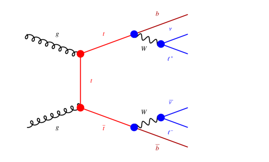
Figure 1: A Feynman diagram for top entanglement at the LHC, with QCD (red) and EW (blue) vertices modified by different $W(p)$ factors.

We compute the dominant partonic process, $t\bar{t}$ productions from gluons $g$. The tree-level amplitude for $g^{a}_{\lambda_{1}}(p_{1})g^{b}_{\lambda_{2}}(p_{2})\to t_{is_{1}}(q_{1})\bar{t}_{j{s_{2}}}(q_{2})$ ($a,b$ are adjoint indices, $i,j$ are color indices, $\lambda_{1,2}$ are gluon helicities, $s_{1,2}$ are top spins), obtained summing the usual $s,t,u$-channel diagrams, is

$$\mathscr{A} = -ig_{3}^{2}\,\epsilon^{\lambda_{1}}_{\mu}(p_{1})\,\epsilon^{\lambda_{2}}_{\nu}(p_{2})\,\overline{\tilde{u}}_{s_{1}}(q_{1})\bigg{\{}\gamma^{\mu}\frac{(T^{a}T^{b})_{ij}}{\not{q}_{1}-\not{p}_{1}-M}\gamma^{\nu}+\gamma^{\nu}\frac{(T^{b}T^{a})_{ij}}{\not{q}_{1}-\not{p}_{2}-M}\gamma^{\mu}+$$

$$+i\frac{f^{abc}}{s}T^{c}_{ij}[\eta^{\mu\nu}(\not{p}_{1}-\not{p}_{2})^{\rho}+\gamma^{\nu}(p_{1}+2p_{2})^{\mu}-\gamma^{\mu}(2p_{1}+p_{2})^{\nu}]\bigg{\}}\tilde{v}_{s_{2}}(q_{2}).$$

This is the standard SM amplitude with spinors replaced by tilted spinors

$$\overline{\tilde{u}}_{s_{1}}(q_{1})=\overline{u}_{s_{1}}(q_{1})\overline{W}(q_{1}),\qquad\tilde{v}_{s_{2}}(q_{2})=W(-q_{2})v_{s_{2}}(q_{2}).$$ (31)

Squaring the amplitude and summing over spins gives factors that reproduce the standard spin sum

$$\sum_{s}{\tilde{u}}_{s}(q)\overline{\tilde{u}}_{s}(q)=W(q)(\not{q}+M)\overline{W}(q)=\not{q}+M=\sum_{s}{{u}}_{s}(q)\overline{{u}}_{s}(q)$$ (32)

$$\sum_{s}{\tilde{v}}_{s}(q)\overline{\tilde{v}}_{s}(q)=-W(-q)(-\not{q}+M)\overline{W}(-q)=\not{q}-M=\sum_{s}{{v}}_{s}(q)\overline{{v}}_{s}(q)$$ (33)

since we assumed that $W$ satisfies eq. (5). So the cross section summed over spins is not affected by $W$. The same happens for the other $q\bar{q}\to t\bar{t}$ partonic processes. So the spin-summed $pp\to t\bar{t}$ cross section at tree level remains the same as in the SM, while the top spin structure is affected. This is manifest in observables processes such as fig. 1 where the spin-summed differential rates for $gg\to t\bar{t}$ and for $t\to b\bar{\ell}\nu$ remain separately unmodified, while the $gg\to b\bar{\ell}\nu\bar{b}\ell\bar{\nu}$ differential rates are modified.

3.1 Spin correlation and entanglement in $pp\to t\bar{t}$

To discuss how the spin structure is modified, we now introduce the standard formalism. Multiple partonic processes contribute to $pp\to t(q_{1},s_{1})\bar{t}(q_{2},s_{2})$ processes, each one with amplitudes $\mathscr{A}(q_{1,2},s_{1,2})$ that depend on the $t$ and $\bar{t}$ momenta $q_{i}$ and spins $s_{i}$. As usual, the squared amplitudes are summed over processes, integrated over their parton densities, averaged over initial-state spins. However, we do not sum over final-state spins, as we want to retain this information. The scattering rates get thereby described by a $4\times 4$ matrix in spin space. It is convenient to write this matrix as the usual total differential cross section $d\sigma(q_{1},q_{2})/dt$ (summed over final-state spins) times a $4\times 4$ density matrix $\rho(q_{1},q_{2})$ in $s_{1},s_{2}$ space normalised as $\,{\rm Tr}\,\rho=1$ that describes the spin composition of each final $t(q_{1})\bar{t}(q_{2})$ state. Furthermore, $\rho$ is usually parameterised in terms of $2\times 2$ Pauli matrices $\sigma_{i}$ as

$$\rho=\frac{1}{4}(\mathbb{1}\otimes\mathbb{1}+(\bm{\sigma}\cdot\bm{S}_{1})\otimes\mathbb{1}+\mathbb{1}\otimes(\bm{\sigma}\cdot\bm{S}_{2})+C_{ij}\,\sigma_{i}\otimes\sigma_{j}).$$ (34)

In this way the first $\mathbb{1}\otimes\mathbb{1}$ term accounts for the usual total cross section; $\bm{S}_{1,2}$ tell the average spins of $t$ and of $\bar{t}$; the spin-correlation matrix $C$ can contain entanglement. For example the spin singlet $t\bar{t}$ state corresponds to $C=-\,{\rm diag}(1,1,1)$. The spin triplet state along the $z$ axis corresponds to $C=\,{\rm diag}(1,1,-1)$.

The new physics introduced in section 2 modifies the SM amplitudes as in eq. (31). This can be conveniently rewritten defining two $2\times 2$ matrices $U(q_{1})$ and $V(q_{2})$ acting on spin indices $s_{1,2}$ as:

$$\tilde{u}_{s_{1}}(q_{1})=\Lambda_{q_{1}}(\Lambda_{q_{1}}^{-1}W(q_{1})\Lambda_{q_{1}})u_{s_{1}}(0)\equiv\Lambda_{q_{1}}U_{s_{1}s_{1}^{\prime}}(q_{1})u_{s^{\prime}_{1}}(0)=U_{s_{1}s^{\prime}_{1}}(q_{1})u_{s^{\prime}_{1}}(q_{1})$$ (35)

and similarly for $v$. In the theory of section 2.2 the matrices $U$ and $V$ do not depend on momenta in frame $S$. In the theories of sections 2.1 and 2.3, $U(q_{1})$ and $V(q_{2})$ are rotations along a rotated $n$, related to $U(0)$ and $V(0)$ by Wigner rotations. In the density matrix language, this means that $\rho$ of eq. (34) gets modified into a $\tilde{\rho}$ where $\mbox{\boldmath$S$}_{1,2}$ and $C$ keep their SM values, and the Pauli matrices for $t$ and for $\bar{t}$ get tilted as

$$\sigma_{i}\to\tilde{\sigma}_{i}=U^{\dagger}\sigma_{i}U\equiv R_{Uij}\sigma_{j},\qquad\sigma_{i}\to\tilde{\sigma}_{i}=V^{\dagger}\sigma_{i}V\equiv R_{Vij}\sigma_{j}.$$ (36)

The above equation means that tilted Pauli matrices can be converted to the usual Pauli basis by noticing that the $U,V$ rotations in spin space induce rotations in space, described by the $3\times 3$ matrices $R_{U}$ and $R_{V}$. So the $\tilde{\rho}$ density matrix can be rewritten in the standard Pauli basis as

$$\tilde{\rho}=\frac{1}{4}(\mathbb{1}\otimes\mathbb{1}+({\bm{\sigma}}\cdot\tilde{\bm{S}}_{1})\otimes\mathbb{1}+\mathbb{1}\otimes({\bm{\sigma}}\cdot\tilde{\bm{S}}_{2})+\tilde{C}_{ij}\,\sigma_{i}\otimes\sigma_{j})$$ (37)

where the $t$ and $\bar{t}$ spins and their correlation matrix get rotated as

$$\tilde{\mbox{\boldmath$S$}}_{1}=R_{U}^{T}\cdot\mbox{\boldmath$S$}_{1},\qquad\tilde{\mbox{\boldmath$S$}}_{2}=R_{V}^{T}\cdot\mbox{\boldmath$S$}_{2},\qquad\tilde{C}=R_{U}^{T}\cdot C\cdot R_{V}.$$ (38)

As expected, the new physics amounts to just rotations of the arbitrary quantization axis, separately for $t$ and $\bar{t}$. These rotations become physical when we assume that the QCD interactions of top quarks are modified by the $U,V$ matrices, while the top weak interactions (responsible for $t$ decays) are not modified. In this way $U,V$ modify, in particular, the angular distributions of leptons $\ell$ in processes where tops are produced via QCD interactions and decay via weak interactions, $t\to b\bar{\ell}\nu$.

3.2 Comparison with Large Hadron Collider data

The lepton angular distributions in the $t\bar{t}$ rest frame have been used by LHC experiments to measure the trace

$$D\equiv\frac{\,{\rm Tr}\,C}{3}=\frac{2}{3}\langle{S}^{2}\rangle-1$$ (39)

of the $pp\to t\bar{t}$ spin correlation matrix, sensitive to the total spin $\bm{S}=\bm{S}_{1}+\bm{S}_{2}$ of the $t\bar{t}$ pair. In order to modify the $D$ observable from its SM value we need to assume that our new physics introduces a relative rotation $U\neq V$ between $t$ and $\bar{t}$. The $\tilde{C}$ matrix is no longer symmetric, implying that CP is broken [14, 15, 16].

The $D$ observable is sensitive, in particular, to spin entanglement. Entanglement is necessarily present if $D<-1/3$ [17] i.e. if $\langle{S}^{2}\rangle<1$. ATLAS confirms top entanglement by measuring, with $140/{\rm fb}$ of integrated luminosity at $\sqrt{s}=13\,{\rm TeV}$ [1],

$$D=-0.547\pm 0.021_{\rm syst}\pm 0.002_{\rm stat}\qquad\hbox{for}\qquad 340\,{\rm GeV}<m_{t\bar{t}}<380\,{\rm GeV}.$$ (40)

The ATLAS analysis restricts the $t\bar{t}$ invariant mass $m_{t\bar{t}}$ to non-relativistic values because, in this limit, the SM predicts that the dominant $gg\to t\bar{t}$ channel gives a maximally entangled spin-singlet state, which corresponds to $D=-1$. Taking into account the finite bin size and the subdominant $q\bar{q}\to t\bar{t}$ channel, the SM prediction [15, 14, 18] computed using the Powheg + Pythia modelling is $D_{\rm SM}=-0.470\pm 0.018_{\rm syst}\pm 0.002_{\rm stat}$ [1]. A second computation, based on the Powheg + Herwig7 modelling, yields an even higher central value [1]. Performing a simple parton-level approximation we find

$$C_{\rm SM}\approx-\,{\rm diag}(0.31,0.45,0.53)\qquad\hbox{i.e.}\qquad D_{\rm SM}\approx-0.43.$$ (41)

The measured $D$ is about $2.8$ standard deviations below the SM predictions, possibly due to neglected non-relativistic QCD processes such as $t\bar{t}$ bound state effects which affect the production of non-relativistic $t\bar{t}$ events [19]. Different computations agree with each other and with data at higher $m_{t\bar{t}}$ away from threshold, where data does not establish top entanglement [1]. A previous CMS analysis could not establish entanglement [4], having not binned on the $t\bar{t}$ invariant mass.

Our new physics effects that modify entanglement depend on the momenta of the produced tops. The $W(p)$ of section 2.3 predict an enhancement for relativistic tops aligned to $n$. For simplicity we focus on the ATLAS sample of non-relativistic tops, eq. (40). Then, in order to significantly modify the $D$ observable, we focus on the theories discussed at points 2. of sections 2.1, 2.2 and 2.3, such that $U$ and $V$ are approximatively opposite rotations with angle $\delta/2$ around the same unit versor $n$. Since the $C_{\rm SM}$ of eq. (41) is roughly proportional to the unit matrix we can neglect how the LHC was oriented (and rotating) with respect to $n$, and approximate $R_{U,V}$ as constant matrices, independent on the scattering geometry. In this approximation eq. (38) can be applied to the average $C$ matrix relevant for ATLAS. Inserting $U=V^{-1}$ and thereby $R_{V}=R_{U}^{T}\equiv R$ in eq. (38), it simplifies into

$$\tilde{C}=R\cdot C_{\rm SM}\cdot R.$$ (42)

A fit to ATLAS data implies the bounds $|\delta|\lesssim 0.4$ at $3\sigma$ roughly independently of the rotation axis $n$. Without loss of generality we can consider a rotation along the spin-quantization $z$ axis. It corresponds a diagonal matrix of phases in the Dirac basis as in eq.s (22), (23) and (29), $W(0)=\,{\rm diag}(e^{i\delta/4},e^{-i\delta/4},e^{-i\delta/4},e^{i\delta/4})$. In its presence, $gg$ collisions produce, in the non-relativistic limit, $t\bar{t}$ pairs with entanglement modified into

$$|\delta\rangle=\frac{e^{-i\delta/2}|t_{\uparrow}\bar{t}_{\downarrow}\rangle-e^{i\delta/2}|t_{\downarrow}\bar{t}_{\uparrow}\rangle}{\sqrt{2}}.$$ (43)

The density matrix $\rho=|\delta\rangle\langle\delta|$ corresponds to the spin correlation matrix

$$\tilde{C}=-\begin{pmatrix}\cos\delta&-\sin\delta&0\cr\sin\delta&\cos\delta&0\cr 0&0&1\end{pmatrix}.$$ (44)

The value of $\tilde{D}=\frac{1}{3}\,{\rm Tr}\tilde{C}=-\frac{1}{3}-\frac{2}{3}\cos\delta$ is increased by $\delta\neq 0$. This shows that $\delta$ affects the entanglement measured by ATLAS. In the limit of a large random $\delta$, quantum coherence is lost giving classical probabilities with no entanglement.

4 Loop effects

In general, new physics in entanglement is expected to affect quantum loops.

However, it is not possible to compute in a model-independent way how loops are affected by a generic loss of entanglement. The reason is that a complete loss of entanglement turns amplitudes into classical probabilities, but loops are amplitudes (such as the loop correction to a particle mass). Specific theories of new physics in entanglement, such as the one we proposed, are needed to study how quantum loops are affected.

To make the discussion concrete, we focus on our phenomenological application. Presumably, quantum loops spread the new physics we introduced into top quarks among all sectors of the theory, while respecting the residual symmetries (the Lorentz sub-groups SO(2), SO(2,1), SIM(2) are considered in section 2) and possibly the form of $W(p)$. A similar outcome was found in a different context: introducing the simplest form of Lorentz-breaking effects — different speeds-of-light $c_{p}$ for different particles $p$ — the $c_{p}$ obey a closed system of Renormalisation Group Equations, computed at one loop in [20].

We assumed that top quarks are affected by a non-local $W(p)$ rotation in spin space that affects differently the top QCD and EW couplings. So deviations from the Standard Model can arise in processes mediated by top loops that involve both QCD and EW interactions. Corrections often arise at two or more loops, and our postulated $W(p)$ breaks rotational invariance. These two characteristics render a technical challenge computing loop corrections to EW physics, Higgs physics, flavour physics, and low-energy physics.

      

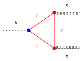
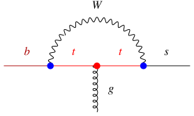
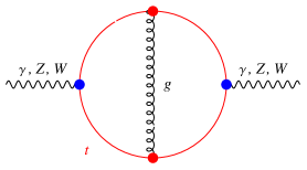
Figure 2: Sample of Feynman diagrams of observed top loops modified by our new physics in entanglement as both QCD (red) and EW (blue) vertices appear.

4.1 Higgs physics

Concerning Higgs physics, the SM predicts that $\Gamma(h\to gg)$, $\Gamma(h\to\gamma\gamma)$, $\Gamma(h\to Z\gamma)$ arise at one loop, mediated by top quark loops (as well as by EW loops). LHC experiments find that these rates agree with the SM within a few tens of $\%$ precision. Our new physics first affects $h\to\gamma\gamma$ and $h\to Z\gamma$ at two loops, so we estimate that experimental bounds are satisfied for $\delta\sim 1$. $\Gamma(h\leftrightarrow gg)$ is less precisely measured from the $pp\to h$ production rate, and it’s affected at one loop. The expression for the diagram in fig. 2 left can be derived from the tree-level expression for $gg\to t(q_{1})\bar{t}(q_{2})$, eq. (3), closing the top loop with an extra top Yukawa interaction, given in the SM by $y_{t}\mathbb{1}$ where $\mathbb{1}$ is the unit matrix in spinor space. The overall effect of our new physics affecting differently QCD vs EW top couplings is replacing $y_{t}\mathbb{1}$ by

$$y_{t}\,W(q_{1})\overline{W}(-q_{2})=y_{t}\,W(k)\overline{W}(k-p),$$ (45)

with $k$ being the loop momentum and $p$ the momentum of the Higgs. Performing the loop integral and the Dirac spinor trace is challenging. The new physics correction trivially vanishes in the limits $p=0$ and $\delta=0$. This allows to estimate a relative correction to $h\leftrightarrow gg$ at least of the order $\delta\Gamma/\Gamma\sim\delta\,M_{h}/M_{t}$, which appears to be within current bounds. This effect vanishes for the $p$-independent $W(p)$ of eq. (14).

4.2 Electroweak precision physics

Coming to EW precision physics, the SM predicts that two EW precision parameters have, at one loop, a strong quadratic sensitivity to the top quark mass: the $\rho\equiv{M_{W}^{2}}/{M_{Z}^{2}\cos^{2}\theta_{\rm W}}$ parameter and the $\epsilon_{b}$ parameter that describes the $Zb_{L}\bar{b}_{L}$ coupling. These parameters are first affected at two loops (e.g. fig. 2 right), as one-loop diagrams involve either QCD or EW interactions, but not both. So the new physics effects are estimated to be below current bounds. In the same way, new physics corrections to the top quark propagator first arises at two loop level. If instead new physics affects bottom quarks too, the $\epsilon_{b}$ parameter is affected at one loop.

4.3 Flavour physics

Coming to flavour physics, measurements of rare decays and oscillations of mostly $K$ and $B$ mesons allowed to test the coefficients of various effective operators that, in the SM, receive contributions from top quarks at one loop level, via box and penguin diagrams. The new physics we introduced mostly affects such coefficients at one higher order than leading SM effects, with the exception of QCD penguins. These first arise and are affected at one loop (fig. 2 middle). Since an external gluon is involved, such operators suffer larger QCD uncertainties. Flavour physics currently is $2-3$ times less sensitive to top quark loops than EW precision tests (see for example the determination of the top quark mass [21]). An exception would arise if the rotation-breaking and/or CP-breaking new physics gives rise to qualitatively new effects, such as chiral enhancements. Qualitatively new effects are however better tested moving from particle-physics experiments to low-energy probes, that we discuss next.

4.4 Low-energy physics

The new physics we introduced affects the photon propagator $\Pi_{\mu\nu}(k)$ first at 2 loops (a sample diagram is shown in the right panel of fig. 2) and the electron propagator at 3 loops. As we are not able of computing these multi-loop diagrams, we limit our discussions to symmetry arguments.

If Lorentz is broken to its smaller SO(2) or SO(2,1) subgroups (as in sections 2.1, 2.2), these residual symmetries have little protective power. In the worst case, loops induce effective operators of the generic form $k_{\mu\nu\alpha\beta}F^{\mu\nu}F^{\alpha\beta}$, with dimension-less coefficients arising at order $k_{\mu\nu\alpha\beta}\sim e^{2}g_{3}^{2}/(4\pi)^{4}$. Some combinations of coefficients $k$ are experimentally constrained down to $10^{-34}$ level by observations of the polarization of sources at cosmological distance [22, 23]. The combination $\delta c$ of $k_{\mu\nu\alpha\beta}$ coefficients that controls the speed of light (compared to the speed of ultra-relativistic electrons or protons) is constrained as $\delta c\lesssim 10^{-15}$ [22]. The SO(2,1)-invariant theory of eq. (14) can be computed finding that it is problematic, as the $p$-independent $W$ modifies the photon vertex $\gamma_{\mu}$ rotating $\gamma_{3}$ into $\gamma_{5}$. The SO(2)-invariant theories of section 2.2 are not easily computed; one might hope that loops preserve their assumed structure (one special frame where new physics induces fixed spin rotations), giving a rotation $R$ of photons and their spin, $\delta\Pi_{\mu\nu}=R_{\mu\mu^{\prime}}R_{\nu\nu^{\prime}}\Pi_{\mu^{\prime}\nu^{\prime}}^{\rm SM}(Rk)$. This would be redefined away from the photon propagator (thereby bypassing bounds on it), leaving effects only in photon interactions.

If Lorentz is broken to its maximal sub-group SIM(2) (as in section 2.3), this residual symmetry forbids most unwanted effects and only allows for a photon mass-like term (of the form $m_{\gamma}^{2}(n_{\mu}F^{\mu\nu}/n^{\alpha}\partial_{\alpha})^{2}$, constrained to be $m_{\gamma}\lesssim 10^{-18}\,{\rm eV}$ [24, 25, 26]) and for a spin-dependent electron mass (of the form $m_{e}\Delta m_{e}\bar{\Psi}\not{n}/(n\cdot\partial)\Psi$, constrained to be $\Delta m_{e}\lesssim 10^{-20}\,{\rm eV}$ [27]). In view of the derivatives at the denominator, such terms should arise from loop integrals that develop IR divergences in the limit of small external momenta. The SIM(2)-invariant theory of eq. (27) gives an IR-divergent modified Dirac propagator, so that the photon mass could arise at one loop. An explicit computation found that the photon remains massless after regularising the IR divergences [28]. We are instead interested in the SIM(2)-invariant theories that preserve spin-summed cross sections, eq. (28) and (29). The assumed exponential structure of $W(p)$ implies that these theories don’t introduce multiplicative IR divergences. In particular, the Dirac propagator keeps its standard form, so there are no one-loop effects. Two-loop effects only contain IR-enhanced spin rotations. Dedicated computations are needed to see if a photon mass is generated at higher loops: the non-local theory is likely non-renormalizable, in the sense that higher loop orders likely modify our assumed benign forms of $W(p)$.

In the worst case, low-energy effects could get naively suppressed by inverse powers of $\Lambda$, by invoking the extra assumption that the new rotation-breaking physics is suppressed by some new physics scale $\Lambda\sim M_{t}$. Such extra (unjustified?) assumption that Lorentz violation grows with energy is often adopted in phenomenological studies, where $\Lambda$ is assumed to be the Planck mass.

Finally, the strongest bound on Lorentz-violating effects (often ignored in the literature) comes from the vacuum energy. The top-quark loop contribution to the energy-momentum tensor $T_{\mu\nu}$ is affected at 3 loops by our new physics. Lorentz-breaking effects would complicate the apparent tuning of the vacuum energies down to its small observed value.

5 Conclusions

We presented a theory of new physics that modifies spin entanglement without altering the total production or decay rates at tree level. As a phenomenological application, this new physics is relevant for tests of $t\bar{t}$ entanglement performed at the LHC, as it affects the $t\bar{t}$ spin correlations and their entanglement, without affecting the spin-summed differential QCD cross sections for $pp\to t\bar{t}$ top quark production, nor the tree-level EW top differential decay rate summed over spins.

In order to accomplish this, we introduced an unconventional theoretical ingredient: a rotation-breaking misalignment $\Psi(x)\to W(i\partial)\Psi(x)$ between the QCD and EW interactions of top quarks. As a result, the polarizations of top quarks with momentum $p$ undergo a $W(p)$ rotation in spinor space when both QCD and EW interactions are involved. A significant new physics effect in the specific entanglement observable tested by ATLAS [1] arises if the breaking of rotational invariance couples in opposite ways to top and anti-top quarks.

In general, one expects that new physics in top quark entanglement also affects processes affected by virtual top quark loops. Such effects have been detected in Higgs physics, EW precision observables, flavor physics, and low-energy experiments. In section 4 we showed that, in various cases, our new physics first enters at higher loop order. The reason is that both QCD and EW interactions must be involved in the loop to have a new physics effect.

The new physics we introduced implies a non-local violation of Lorentz invariance. We attempted to keep this violation below experimental constraints by postulating that, at tree level, it exclusively influences top quarks. However, at loop level, this violation extends to other particles better tested than tops. In order to alleviate these Lorentz-violating effects, we assumed specific benign forms for the $W(p)$ function, that break Lorentz and the space-time discrete symmetries to different sub-groups, as listed in table 1.

• In section 2.2 we break Lorentz almost completely, but adjust the tree-level $W(p)$ to minimise the physical impact of broken boosts. One rest frame is special just because, in it, the new physics that rotates spin is not affected by Wigner rotations.

• In section 2.3 we break Lorentz to its maximal SIM(2) sub-group that contains all boosts (mixed with rotations): this unbroken Lorentz sub-group is powerful enough that no rest frame becomes special. The speed of light $c$ remains universal, and most unobserved Lorentz-violating effects are similarly controlled by the residual symmetry. Our findings provide new realizations of (necessarily non-local) theories invariant under SIM(2).

However, the resulting theories are likely non-renormalizable: at some level quantum corrections might transform our assumed $W(p)$ functions into a more problematic form. In such a case, the applicability of the theories under consideration would become limited primarily to tree-level phenomenological applications, such as in the domain of top physics.

Acknowledgements

We thank Daniele Barducci and Gino Isidori.

References

- [1] ATLAS Collaboration, ‘Observation of quantum entanglement in top-quark pairs using the ATLAS detector’ [\IfSubStr2311.07288:InSpire:2311.07288arXiv:2311.07288].
- [2] T. Stelzer, S. Willenbrock, ‘Spin correlation in top quark production at hadron colliders’, Phys.Lett.B 374 (1996) 169 [\IfSubStrhep-ph/9512292:InSpire:hep-ph/9512292arXiv:hep-ph/9512292].
- [3] A.J. Barr, M. Fabbrichesi, R. Floreanini, E. Gabrielli, L. Marzola, ‘Quantum entanglement and Bell inequality violation at colliders’ [\IfSubStr2402.07972:InSpire:2402.07972arXiv:2402.07972].
- [4] CMS Collaboration, ‘Measurement of the top quark polarization and spin correlations using dilepton final states in proton-proton collisions at 13 TeV’, Phys.Rev.D 100 (2019) 072002 [\IfSubStr1907.03729:InSpire:1907.03729arXiv:1907.03729].
- [5] A. Einstein, B. Podolsky, N. Rosen, ‘Can quantum mechanical description of physical reality be considered complete?’, Phys.Rev. 47 (1935) 777.
- [6] E. Schrodinger, ‘Discussion of probability relations between separated systems’, Proceedings of the Cambridge Philosophical Society 31 (1935) 555.
- [7] M.M. Altakach, P. Lamba, F. Maltoni, K. Mawatari, K. Sakurai, ‘Quantum information and CP measurement in at future lepton colliders’, Phys.Rev.D 107 (2023) 093002 [\IfSubStr2211.10513:InSpire:2211.10513arXiv:2211.10513].
- [8] R. Aoude, E. Madge, F. Maltoni, L. Mantani, ‘Quantum SMEFT tomography: Top quark pair production at the LHC’, Phys.Rev.D 106 (2022) 055007 [\IfSubStr2203.05619:InSpire:2203.05619arXiv:2203.05619].
- [9] M. Fabbrichesi, R. Floreanini, E. Gabrielli, ‘Constraining new physics in entangled two-qubit systems: top-quark, tau-lepton and photon pairs’, Eur.Phys.J.C 83 (2023) 162 [\IfSubStr2208.11723:InSpire:2208.11723arXiv:2208.11723].
- [10] For a recent work see R. Shaw, ‘The subgroup structure of the homogeneous Lorentz group’, Quarterly J. of Math. 2 (1970) 101. See also ‘Subgroups of the Lorentz group’ in wikipedia.
- [11] A.G. Cohen, S.L. Glashow, ‘Very special relativity’, Phys.Rev.Lett. 97 (2006) 021601 [\IfSubStrhep-ph/0601236:InSpire:hep-ph/0601236arXiv:hep-ph/0601236].
- [12] D.V. Ahluwalia, S.P. Horvath, ‘Very special relativity as relativity of dark matter: The Elko connection’, JHEP 11 (2010) 078 [\IfSubStr1008.0436:InSpire:1008.0436arXiv:1008.0436].
- [13] A.G. Cohen, S.L. Glashow, ‘A Lorentz-Violating Origin of Neutrino Mass?’ [\IfSubStrhep-ph/0605036:InSpire:hep-ph/0605036arXiv:hep-ph/0605036].
- [14] W. Bernreuther, A. Brandenburg, ‘Tracing CP violation in the production of top quark pairs by multiple TeV proton proton collisions’, Phys.Rev.D 49 (1994) 4481 [\IfSubStrhep-ph/9312210:InSpire:hep-ph/9312210arXiv:hep-ph/9312210].
- [15] M. Baumgart, B. Tweedie, ‘A New Twist on Top Quark Spin Correlations’, JHEP 03 (2013) 117 [\IfSubStr1212.4888:InSpire:1212.4888arXiv:1212.4888].
- [16] W. Bernreuther, D. Heisler, Z.-G. Si, ‘A set of top quark spin correlation and polarization observables for the LHC: Standard Model predictions and new physics contributions’, JHEP 12 (2015) 026 [\IfSubStr1508.05271:InSpire:1508.05271arXiv:1508.05271].
- [17] Y. Afik, J.R.M. de Nova, ‘Entanglement and quantum tomography with top quarks at the LHC’, Eur.Phys.J.Plus 136 (2021) 907 [\IfSubStr2003.02280:InSpire:2003.02280arXiv:2003.02280].
- [18] P. Uwer, ‘Maximizing the spin correlation of top quark pairs produced at the Large Hadron Collider’, Phys.Lett.B 609 (2005) 271 [\IfSubStrhep-ph/0412097:InSpire:hep-ph/0412097arXiv:hep-ph/0412097].
- [19] Y. Kiyo, J.H. Kuhn, S. Moch, M. Steinhauser, P. Uwer, ‘Top-quark pair production near threshold at LHC’, Eur.Phys.J.C 60 (2009) 375 [\IfSubStr0812.0919:InSpire:0812.0919arXiv:0812.0919].
- [20] G.F. Giudice, M. Raidal, A. Strumia, ‘Lorentz Violation from the Higgs Portal’, Phys.Lett.B 690 (2010) 272 [\IfSubStr1003.2364:InSpire:1003.2364arXiv:1003.2364].
- [21] G.F. Giudice, P. Paradisi, A. Strumia, ‘Indirect determinations of the top quark mass’, JHEP 11 (2015) 192 [\IfSubStr1508.05332:InSpire:1508.05332arXiv:1508.05332].
- [22] V.A. Kostelecky, N. Russell, ‘Data Tables for Lorentz and CPT Violation’, Rev.Mod.Phys. 83 (2011) 11 [\IfSubStr0801.0287:InSpire:0801.0287arXiv:0801.0287].
- [23] R. Gerasimov, P. Bhoj, F. Kislat, ‘New Constraints on Lorentz Invariance Violation from Combined Linear and Circular Optical Polarimetry of Extragalactic Sources’, Symmetry 13 (2021) 880 [\IfSubStr2104.00238:InSpire:2104.00238arXiv:2104.00238].
- [24] S. Cheon, C. Lee, S.J. Lee, ‘SIM(2)-invariant Modifications of Electrodynamic Theory’, Phys.Lett.B 679 (2009) 73 [\IfSubStr0904.2065:InSpire:0904.2065arXiv:0904.2065].
- [25] J. Alfaro, V.O. Rivelles, ‘Non Abelian Fields in Very Special Relativity’, Phys.Rev.D 88 (2013) 085023 [\IfSubStr1305.1577:InSpire:1305.1577arXiv:1305.1577].
- [26] J. Alfaro, V.O. Rivelles, ‘Very Special Relativity and Lorentz Violating Theories’, Phys.Lett.B 734 (2014) 239 [\IfSubStr1306.1941:InSpire:1306.1941arXiv:1306.1941].
- [27] J.J. Fan, W.D. Goldberger, W. Skiba, ‘Spin dependent masses and Sim(2) symmetry’, Phys.Lett.B 649 (2007) 186 [\IfSubStrhep-ph/0611049:InSpire:hep-ph/0611049arXiv:hep-ph/0611049].
- [28] A. Dunn, T. Mehen, ‘Implications of symmetry for SIM(2) invariant neutrino masses’ [\IfSubStrhep-ph/0610202:InSpire:hep-ph/0610202arXiv:hep-ph/0610202].