\marginsize

1.75cm1.75cm0.5cm0.5cm

DNN
Deep Neural Network
ODE
Ordinary Differential Equation
SPDE
Stochastic Partial Differential Equation
FNN
Feed-forward Neural Network
CNN
Convolutional Neural Network
DP
Dynamic Programming
LSTM
Long-Short Term Memory
FC
Fully Connected
DDP
Differential Dynamic Programming
HJB
Hamilton-Jacobi-Bellman
PDE
Partial Differential Equation
PI
Path Integral
NN
Neural Network
SOC
Stochastic Optimal Control
RL
Reinforcement Learning
MPC
Model Predictive Control
IL
Imitation Learning
RNN
Recurrent Neural Network
DL
Deep Learning
SGD
Stochastic Gradient Descent
SDE
Stochastic Differential Equation
VRL
Variational Reinforcement Learning
IDVRL
Infinite Dimensional Variational Reinforcement Learning
1D
1-dimensional
2D
2-dimensional
ROM
Reduced Order Model
SDE
Stochastic Ordinary Differential Equation (ODE)

  Learning with SASQuaTCh: a Novel Variational Quantum Transformer Architecture with Kernel-Based Self-Attention
 

Ethan N. Evans, Matthew Cook, Zachary P. Bradshaw, and Margarite L. LaBorde
Naval Surface Warfare Center, Panama City Division
Corresponding author. Email: eevans89@gmail.com
Abstract

The widely popular transformer network popularized by the generative pre-trained transformer (GPT) has a large field of applicability, including predicting text and images, classification, and even predicting solutions to the dynamics of physical systems. In the latter context, the continuous analog of the self-attention mechanism at the heart of transformer networks has been applied to learning the solutions of partial differential equations and reveals a convolution kernel nature that can be exploited by the Fourier transform. It is well known that many quantum algorithms that have provably demonstrated a speedup over classical algorithms utilize the quantum Fourier transform. In this work, we explore quantum circuits that can efficiently express a self-attention mechanism through the perspective of kernel-based operator learning. In this perspective, we are able to represent deep layers of a vision transformer network using simple gate operations and a set of multi-dimensional quantum Fourier transforms. We analyze the computational and parameter complexity of our novel variational quantum circuit, which we call Self-Attention Sequential Quantum Transformer Channel (SASQuaTCh), and demonstrate its utility on simplified classification problems.

Introduction and Related Work

Quantum computing has arisen as an alternate computing paradigm in which the properties of quantum theory are leveraged to potentially outperform classical devices on certain problems, including prime factorization [1] and unstructured search problems [2]. While such algorithms will have profound consequences in areas such as cryptography [3] when a machine capable of running them becomes available, that time has not yet come. In recent years, focus has been on so-called noisy intermediate scale quantum (NISQ) devices [4] and finding potential uses for these devices today. A promising contender is the rising field of quantum machine learning [5], which intends to combine the success of machine learning algorithms with the framework of quantum computing to produce better machine learning models by leveraging properties such as superposition and entanglement.

A recent development in classical machine learning has been the introduction of the transformer architecture [6] in 2017 by Vaswani et al., which first saw great success in natural language processing (NLP), the problem of training machines to interpret and process human languages. These large language models have experienced an explosion in parameter growth, first growing by seven orders of magnitude from 1950 to 2018, followed by a massive five orders of magnitude in just four years from 2018 to 2022 [7]. Since its advent, applications have been found for transformers outside of NLP, including image recognition [8], speech recognition [9], and predicting dynamical systems [10]. The success of this architecture has been largely attributed to its use of a multi-head attention mechanism performing scaled dot-product attention in each unit, and this involves learning three weight matrices, known as the query, key, and value weights for each attention head. This mechanism, along with a positional encoding, allows the model to understand the context of a component of the input in relation to the remaining components. However, in 2021, Lee-Thorp et al. [11] showed that replacing the self-attention sublayers with standard, unparameterized Fourier transforms retains 92-97% of the accuracy of state of the art Bidirectional Encoder Representations from Transformers (BERT) [12] models on the General Language Understanding Evaluation (GLUE) benchmark, while also training 80% faster on GPUs and 70% faster on TPUs at standard 512 input lengths. The lack of trainable parameters in the Fourier transform also reduces the memory footprint of the model.

In this work, we implement a quantum vision transformer inspired by the Fourier Neural Operator [13], the Adaptive Fourier Neural Operator [14], and the FourCastNet [15]. These models make use of the observation that the scaled dot product self-attention mechanism can be represented by a convolution against a stationary kernel. To construct our model, we make use of the quantum Fourier transform (QFT), which can be implemented efficiently on a quantum computer. The QFT performs a version of channel mixing, and enables one to easily perform token mixing of a sequence of tokens via a variational quantum circuit acting as a kernel in the Fourier domain. We call our overall circuit Self-Attention Sequential Quantum Transformer Channel (SASQuaTCh). While we use image classification to evaluate our approach, this approach is very general in its applicability to sequence data of any form (e.g. solutions to dynamical systems, natural language processing, and time series data).

Our approach leverages the QFT, which manipulates the $2^{n}$ complex amplitudes in an $n$-qubit state with $O(n^{2})$ Hadamard gates and controlled phase shift gates, although an efficient approximation can be achieved with $O(n\log(n))$ gates, assuming that controlled phases are native to the quantum computing architecture [16]. Meanwhile, the fast Fourier transform on a vector with $2^{n}$ coefficients takes $O(n2^{n})$ operations, so that an apparent exponential speedup has been achieved. However, it should be noted that the Fourier transforms are being taken in different domains. Indeed, in the classical setting, one has access to all the resulting coefficients of the computation, while in the quantum setting, the coefficients are hidden by the collapse of the wavefunction upon measurement and can only be estimated by repeatedly running the QFT procedure. Moreover, given a sequence of data, performing the QFT requires embedding the data into the amplitudes of a quantum state, which is nontrivial and likely cannot be done efficiently in general (although there are some classes of states for which an efficient preparation is known, e.g. uniform superpositions [17, 18]).

It should be noted that the idea of implementing the self-attention mechanism present in the transformer architecture on a quantum device was taken up in [19] with the introduction of the Quantum Self-Attention Neural Network (QSANN). As in the classical case, the quantum self-attention mechanism employed in QSANN makes use of trainable weights broken down into the query, key, and value parts, and these components are used to evolve the embedded state which is then measured. Notably, these measurement outputs are used to classically compute the self-attention mechanism. Thus, any quantum advantage from QSANN must come from the calculation of the query, key, and value components. This is in contrast to the approach presented here, in which the entirety of the self-attention mechanism is performed on a quantum device. Additional efforts to implement a GPT-style algorithm were proposed while this manuscript was in preparation [20]; however, the implementation in that work requires extensive gate operations and does not utilize the kernel-based self-attention framework as done here. Furthermore, we are able to provide proof-of-concept implementations of our work which are not feasible for other, similar works at this time.

The remainder of this work is organized as follows. In Section 2, we give a brief discussion of the relevant background, including a primer on quantum machine learning and the basics of the self-attention mechanism and related works which attempt to implement a quantum analog. In Section 3 we present the mathematical background for our proposed quantum Fourier vision transformer, and in Section 4 we implement the model with quantum circuits. Finally, we give concluding remarks in Section 5.

Preliminaries & Notation

Before moving on, we review some of the necessary background on quantum machine learning, as well as the classical self-attention and multi-head attention networks used in transformers. These ideas will be united to create a fully quantum version of self-attention by observing that the classical self-attention mechanism can be written as a convolution against a stationary kernel and applying the convolution theorem to write it in a form conducive to quantum circuit implementation. The SASQuaTCh architecture is a quantum transformer model which utilizes this quantum self-attention mechanism, making the background in the next subsections paramount to an understanding of the architecture.

Quantum Machine Learning

Quantum machine learning refers to any of a number of approaches which attempt to exploit the properties of quantum theory to create machine learning models. Here we focus on a method based on variational quantum circuits. By allowing trainable parameters into its design, the circuit can learn to mimic the value of a function which we wish to estimate. Indeed, suppose we are given a data set $\mathcal{S}=\{(x_{i},y_{i})\}$ consisting of pairs of data points $x_{i}$ drawn from some data space $\mathcal{R}$ with labels $y_{i}$ in some set $\mathcal{L}$, and assume there is a function $f:\mathcal{R}\to\mathcal{L}$ which correctly maps a data point to its associated label, i.e. $f(x_{i})=y_{i}$ for all $i$. It is then desirable to know $f$ so that given a data point $x\in\mathcal{R}$, the label $f(x)\in\mathcal{L}$ can be predicted. Our goal is therefore to approximate $f$ using a variational quantum circuit (VQC). Typically $f$ is approximated by a set of variational quantum gates, expressed as parametrized unitary operators $U_{\theta}$, where $\theta\in[0,2\pi)$ are a set of parameters which are iteratively optimized via any number of optimization algorithms. In what follows, we denote $n$ tensor products of a gate $U$ acting on some Hilbert space ${\cal H}$ by $U^{\otimes n}$.

The construction of the VQC begins with an embedding of the data into a Hilbert space, and this alone is a nontrivial step, as the choice of embedding can have profound consequences on the trainability of the model [5, 21] (see also [22] for robustness results). Possibly the most obvious embedding is the basis embedding, where the binary representation $B(x)$ of the data point $x$ is embedded into a Hilbert space by mapping $x$ to the computational basis state $|B(x)\rangle$. However, this approach is extremely resource inefficient, as the necessary number of qubits is equivalent to the number of bits in the binary representation. On the opposite end of the spectrum is the amplitude embedding, where the data features are encoded in the coefficients of a quantum state. Since there are $2^{n}$ coefficients in an $n$-qubit quantum state, the required number of qubits to implement this embedding is $O(\log(n))$, where $n$ is the number of features in $x$. However, the problem of preparing an arbitrary state is thought to be hard, so that the actual implementation of this embedding is difficult to perform in practice. Somewhere in the middle is the so-called angle embedding, where the data features are encoded in the angles of $n$ rotation operators which are then applied to the $|0\rangle^{\otimes n}$ state. The angle embedding therefore requires $O(n)$ qubits. Another option is to train the embedding to maximally separate data classes in a Hilbert space as suggested by Lloyd et al. [23]. For now, we will assume that an embedding $\mathcal{E}:\mathcal{R}\to\mathcal{U}(\mathcal{H})$ has been chosen, where ${\cal U}({\cal H})$ is the space of unitary operators on $\mathcal{H}$.

Typically, the next step is to apply a parameterized unitary operator $U_{\theta}$, which can have many forms, but generally this operation should entangle the data qubits together so that they interact with one another. This allows information to be shared between the data qubits, thereby enhancing trainability. Note that the QFT, although unparameterized, was shown to have this property [24]. The final step in the variational circuit is to make a measurement with respect to an observable ${\cal O}$ which is then used to predict the label associated to the given data point. The expected value of this circuit is given by

$$h_{\theta}(x)={\mathrm{Tr}}\left[U_{\theta}(\mathcal{E}(x)|0\rangle\!\!\langle 0|\mathcal{E}(x)^{\dagger})U^{\dagger}_{\theta}\mathcal{O}\right],$$ (1)

where ${\cal O}$ is some chosen observable, ${\cal E}$ is an embedding, and $U_{\theta}$ is the parameterized unitary at the heart of the VQC with parameters $\theta\in\mathbb{R}^{m}$. We interpret eq. 1 as an estimate of the function $f$, and our goal is to minimize the error in this estimation.

The VQC is trained using any of a number of optimization schemes. Early optimization methods include the Nelder-Mead [25] and other zeroth-order or direct search methods; however, these have largely been replaced by methods that at least approximate the gradient of the variational circuit with respect to its trainable parameters. Notably, the parameter-shift rule and its stochastic variant are first-order optimization methods which allow us to recover the exact analytic gradient by simply running the circuit with the parameters shifted up and down [26, 27, 28]; however, it requires $O(3mr)$ evaluations of the circuit, where $m$ is the number of variational parameters and $r$ is the number of shots used to approximate the expectation. A popular alternative is the Simultaneous Perturbation Stochastic Approximation (SPSA) method [29], which is a quasi-first order method that approximates the gradient via a random simultaneous shift of all parameters, and thus only requires $O(r)$ evaluations of the circuit. Variants of these methods incorporate the quantum natural gradient via the quantum Fisher information matrix, as in QN-SPSA [30], incorporate approximate second-order (Hessian) information as in 2SPSA [31] or L-BFGS [32], or incorporate well-established classical machine learning techniques such as adaptive learning rates or momentum [33].

Classical Self-Attention and Multi-Head Attention Networks

The transformer network architecture has quickly become a staple in advanced machine learning. The primary mechanism is known as self-attention, or scaled dot product attention, and the primary data type that transformers are applied to is sequence data. Let $\{x_{s}\in\mathbb{R}^{d}\}_{s=1}^{N}$ be a sequence of $N$ tokens representing the input data. As originally introduced in [6], the self-attention mechanism is given by

$\displaystyle a_{s,j}$ $\displaystyle=\frac{\exp\big{(}x_{s}^{\mathsf{T}}W_{q}^{\mathsf{T}}W_{k}x_{j}\big{)}}{\sum_{l=1}^{S}\exp\big{(}x_{s}^{\mathsf{T}}W_{q}^{\mathsf{T}}W_{k}x_{l}\big{)}}$ (2a)
$\displaystyle y_{s}$ $\displaystyle=\text{Att}(x_{s}):=\sum_{j=1}^{S}a_{s,j}W_{v}x_{j},$ (2b)

where $W_{q},W_{k},W_{v}\in\mathbb{R}^{d\times d}$ are the trainable query, key, and value matrices, respectively. Here, the output $y_{s}$ is a sequence of the same shape as the input $x_{s}$, and is calculated by weighted sums of input elements. The normalized exponential in eq. 2a applies an asymmetric weighting of the input sequence, and can be represented as a scaled dot product. Let $\langle\cdot,\cdot\rangle$ denote an inner product in $\mathbb{R}^{d}$. Then eq. 2a can be written as

$$a_{s,j}=\frac{\exp\big{(}\langle W_{q}x_{s},W_{k}x_{j}\rangle\big{)}}{\sum_{l=1}^{S}\exp\big{(}\langle W_{q}x_{s},W_{k}x_{l}\rangle\big{)}}$$ (3)

This normalized exponential is typically referred to in literature as the softmax activation function, defined by

$$\text{softmax}(z):=\frac{e^{z}}{\sum_{j=1}^{N}e^{z_{j}}}.$$ (4)

With this, the coefficients of the attention are formulated concisely as

$$a_{s,j}=\text{softmax}\left(\frac{\langle W_{q}x_{s},W_{k}x_{j}\rangle}{\sqrt{d}}\right).$$ (5)

In many applications of transformer networks, a set of self-attention operations are typically performed in parallel, each with a different set of weights $W_{q}^{i}$, $W_{k}^{i}$, $W_{v}^{i}$, for $i=1,\dots,h$. This is referred to as multi-head attention [6] and results in parallel projections into a variety of subspaces which are then combined as a linear combination. Multi-head attention is expressed mathematically as
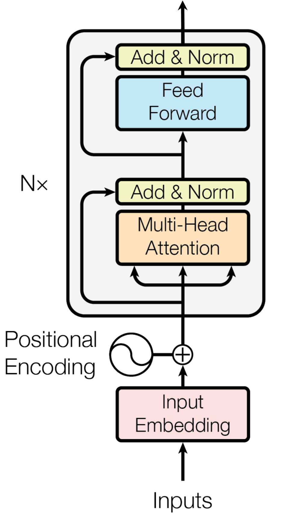
$$\textnormal{MultiHead}(x)=\textnormal{Concat}(y_{s}^{1},\ldots,y_{s}^{h})W_{o},$$

where $h$ is the number of heads, and all weights $W_{q}^{i}$, $W_{k}^{i}$, $W_{v}^{i}$, $i=1,\dots,h$, and $W_{o}$ are trainable. This multi-head attention mechanism simultaneously grants the model access to different subspaces at different positions in the input sequence. See fig. 1 for a visual representation of a transformer model with self-attention.

Refer to caption
Figure 1: Visual representation of a transformer model with self-attention. This figure is taken with permission from [6].

The idea of applying the self-attention mechanism as part of a quantum machine learning architecture was most notably introduced in the Quantum Self-Attention Neural Network (QSANN) [19]. Therein, the authors apply several quantum circuit ansatze, each geared toward a specific component of the self-attention mechanism: an ansatz for embedding each vector of the classical sequence data into a quantum state, an ansatz for the query, an ansatz for the key, and an ansatz for the value. The query, key, and value ansatze each returns a measurement output (i.e. a classical value), and the self-attention is computed classically on these measurement outputs. The sequence is handled by distributing the set of ansatze to each element of the sequence. In the case of ansatze that have trainable parameters (i.e. the query, key, and value circuits), the parameters are frozen when applied across elements of the sequence. The QSANN approach modifies the self-attention mechanism in eq. 2 for use in quantum circuits.

Let $|\psi_{s}\rangle$ denote the encoded classical input sequence

$$|\psi_{s}\rangle:={\cal E}(x_{s})|0\rangle^{\otimes d},$$ (6)

where ${\cal E}$ is a quantum circuit ansatz that acts on an element of the input sequence $x_{s}\in\mathbb{R}^{d}$, $s=1,\dots,N$. Three quantum ansatze $U_{q},U_{k},U_{v}$ with parameters $\theta_{q},\theta_{k},\theta_{v}$ are used to represent the query, key, and value of a given layer. Denote $\langle\mathcal{O}_{q}\rangle_{s}$ and $\langle\mathcal{O}_{k}\rangle_{s}$ the measurement outcomes of the associated query and key parts with respect to some observables $\mathcal{O}_{q}$ and $\mathcal{O}_{k}$, respectively, given explicitly as

$\displaystyle\langle\mathcal{O}_{q}\rangle_{s}$ $\displaystyle:=\langle\psi_{s}|U_{q}^{\dagger}(\theta_{q})\mathcal{O}_{q}U_{q}(\theta_{q})|\psi_{s}\rangle$ (7)
$\displaystyle\langle\mathcal{O}_{k}\rangle_{s}$ $\displaystyle:=\langle\psi_{s}|U_{k}^{\dagger}(\theta_{k})\mathcal{O}_{k}U_{k}(\theta_{k})|\psi_{s}\rangle.$ (8)

The value calculation differs from the query and key. Since $x_{s}\in\mathbb{R}^{d}$, we require the same dimensionality in the output $y_{s}\in\mathbb{R}^{d}$. Thus the value part is represented by a $d$-dimensional vector given by

$$v_{s}:=[\langle\mathcal{O}_{v}^{(1)}\rangle_{s},\;\langle\mathcal{O}_{v}^{(2)}\rangle_{s},\;\dots,\;\langle\mathcal{O}_{v}^{(d)}\rangle_{s}]^{\mathsf{T}}$$ (9)

where $\langle\mathcal{O}_{v}^{(j)}\rangle_{s}:=\langle\psi_{s}|U_{v}^{\dagger}(\theta_{v})\mathcal{O}_{v}^{(j)}U_{v}(\theta_{v})|\psi_{s}\rangle$. The classical output is given by

$\displaystyle y_{s}$ $\displaystyle=x_{s}+\sum_{j=1}^{N}\tilde{\alpha}_{s,j}\;v_{j}$ (10a)
$\displaystyle\tilde{\alpha}_{s,j}$ $\displaystyle=\text{softmax}\Big{(}-\big{(}\langle\mathcal{O}_{q}\rangle_{s}-\langle\mathcal{O}_{k}\rangle_{j}\big{)}^{2}\Big{)}=\frac{e^{-\big{(}\langle\mathcal{O}_{q}\rangle_{s}-\langle\mathcal{O}_{k}\rangle_{j}\big{)}^{2}}}{\sum_{m=1}^{N}e^{-\big{(}\langle\mathcal{O}_{q}\rangle_{s}-\langle\mathcal{O}_{k}\rangle_{m}\big{)}^{2}}}$ (10b)

where it should be noted the input is added to the output as a residual term as in [6].

Notably, the QSANN approach deviates from the classical self-attention in how the self-attention coefficients are calculated. The self-attention coefficients in eq. 10b do not use the standard inner product, but rather use the so-called Gaussian Projected Quantum Self-Attention (GPQSA). The authors argue that in the case of the QSANN circuit, the rotations caused by the inner product make it difficult to correlate states that are far away, and since the parts of the coefficients are each classical measurement outcomes, their difference can be easily obtained and more easily correlates distant quantum states.

Another key take-away from this method is that while each of the components of the self-attention are obtained via variational quantum circuits, the actual self-attention mechanism is computed classically. Thus any potential quantum advantage of the QSANN approach must be derived from the individual component circuits that calculate the query, key, and value. Furthermore, as the intention of the QSANN architecture is to serve as a layer (in the machine learning sense) that is repeated $L$ times, one must repeatedly encode the classical $y_{s}$ from the previous layer in a quantum circuit and leave the quantum circuit to obtain the query, key, and value at the end of each layer. This may introduce substantial overhead, and may also be deleterious to the small time-complexities that one expects from the evaluation of a quantum circuit. This provides strong motivation for identifying novel variational quantum circuits that can handle sequence data and perform self-attention, while not having to repeatedly leave the quantum circuit.

Kernel Convolution and Visual Attention Networks

In the seemingly unrelated field of predicting solutions of complex spatiotemporal systems, the use of visual attention has gained popularity, primarily due to the Fourier Neural Operator (FNO) [13] and the follow-on Adaptive Fourier Neural Operator (AFNO) [14]. These methods coalesce in a neural network called FourCastNet [15] that achieves state-of-the-art prediction accuracy on weather systems. Therein, the task is to generate solutions from a spatiotemporal process that can be written as a partial differential equation. While seemingly weather system prediction and natural language processing (as in [6, 19]) are completely unrelated tasks, they are unified by underlying sequence data. Indeed, a large variety of tasks involve sequence data, and this is where transformer networks often excel.

The innovation presented in [13, 14, 15] is a perspective that the scaled dot product self-attention mechanism in [6] can be represented as an integral transform defined by a stationary kernel and treated with the convolution theorem. The self-attention mechanism is represented in a compact tensor notation form. Let $x\in\mathbb{R}^{N\times d}$ denote the entire sequence by concatenation $[x_{1},x_{2},\dots,x_{N}]^{\mathsf{T}}$ such that the subscript notation used earlier denotes index $s$ of the sequence, and similarly for $y\in\mathbb{R}^{N\times d}$ and $a\in\mathbb{R}^{N\times N}$. The attention function may be concisely expressed as

$\displaystyle y_{s}$ $\displaystyle=\text{Att}(x_{s}):=\sum_{s^{\scaleobj{0.8}{\prime}}=1}^{N}\text{softmax}\left(\frac{\big{\langle}W_{q}x_{s},W_{k}x_{s^{\scaleobj{0.8}{\prime}}}\big{\rangle}}{\sqrt{d}}\right)W_{v}x_{s^{\scaleobj{0.8}{\prime}}}$
$\displaystyle=\sum_{s^{\scaleobj{0.8}{\prime}}=1}^{N}a_{s,s^{\scaleobj{0.8}{\prime}}}W_{v}x_{s^{\scaleobj{0.8}{\prime}}}$ (11)

In this context self-attention can be described by the action of the asymmetric $d\times d$ matrix-valued kernel

$$\kappa_{s,s^{\scaleobj{0.8}{\prime}}}:=a_{s,s^{\scaleobj{0.8}{\prime}}}W_{v},$$ (12)

so that self-attention can be viewed as a sum against this kernel

$$\text{Att}(x_{s})=\sum_{s^{\scaleobj{0.8}{\prime}}=1}^{N}\kappa_{s,s^{\scaleobj{0.8}{\prime}}}x_{s^{\scaleobj{0.8}{\prime}}},\qquad\forall s=1,\dots,N.$$ (13)

If $\kappa$ is a stationary kernel, then there exists a $\hat{\kappa}$ such that $\kappa_{s,s^{\scaleobj{0.8}{\prime}}}=\hat{\kappa}_{s-s^{\scaleobj{0.8}{\prime}}}$, and eq. 13 becomes a global convolution

$$\text{Att}(x_{s})=\sum_{s^{\scaleobj{0.8}{\prime}}=1}^{N}\hat{\kappa}_{s-s^{\scaleobj{0.8}{\prime}}}x_{s^{\scaleobj{0.8}{\prime}}},\qquad\forall s=1,\ldots,N.$$ (14)

Finally, leveraging the convolution theorem, one has

$$\text{Att}\big{(}x_{s}\big{)}={\cal F}^{-1}\Big{(}{\cal F}(\hat{\kappa}){\cal F}(x)\Big{)}_{s}\qquad\forall s=1,\dots,N,$$ (15)

where ${\cal F},{\cal F}^{-1}$ are the forward and inverse Fourier transform, respectively. Note that any transform that satisfies the convolution theorem may be used in place of the Fourier transform. In the AFNO network, this is implemented via a complex-valued weight tensor $W:=DFT(\kappa)\in\mathbb{C}^{N\times d\times d}$ using the Discrete Fourier Transform (DFT) per token as follows:

  1. i)

    Token mixing:            $z_{m,n}=\Big{[}DFT(X)\Big{]}_{m,n}$

  2. ii)

    Channel mixing:         $\tilde{z}_{m,n}=W_{m,n}\;z_{m,n}$

  3. iii)

    Token de-mixing:       $y_{m,n}=\Big{[}IDFT(\tilde{Z})\Big{]}_{m,n}$

Two key innovations are occurring here. First, by assuming the weights are already in the Fourier domain, one does not need to take the Fourier transform of the weight matrix. Since these are trainable weights anyway, this is an appropriate assumption. Secondly, token mixing is performed by means of the Fourier transform, which has well-established value in the context of many types of data including image data. Unlike the standard perspective of self-attention, this straightforward implementation of the self-attention mechanism by means of eq. 15 has a natural extension to quantum circuits.

Continuous Kernel Integral

As an aside, the kernel summation can be extended to the continuous integral setting [13]. While this may seem unnecessary in the context of finite Hilbert spaces as in qubit systems, it is particularly relevant to uncountably infinite Hilbert spaces as in continuous variable quantum computing. Let ${\cal D}\subset\mathbb{R}^{2}$ be a bounded domain and let ${\cal H}_{d}=\{f:{\cal D}\rightarrow\mathbb{R}^{d}\}$ be a Hilbert space of functions from ${\cal D}$ to $\mathbb{R}^{d}$, so that $X$ can be viewed as a spatial function $X\in{\cal H}_{d}$. Define the integral transform ${\cal K}:{\cal H}_{d}\rightarrow{\cal H}_{d}$ by

$${\cal K}\big{(}X\big{)}(s)=\int_{D}\kappa(s,s^{\scaleobj{0.8}{\prime}})X(s^{\scaleobj{0.8}{\prime}}){\mathrm{d}}s^{\scaleobj{0.8}{\prime}}\qquad\forall s\in D,$$ (16)

where $\kappa:D\times D\rightarrow\mathbb{R}^{d\times d}$ is a continuous kernel function. If $\kappa$ is once again assumed to be stationary $\kappa(s,s^{\scaleobj{0.8}{\prime}})=\kappa(s-s^{\scaleobj{0.8}{\prime}})$, then eq. 16 becomes a global convolution

$${\cal K}\big{(}X\big{)}(s)=\int_{D}\kappa(s-s^{\scaleobj{0.8}{\prime}})X(s^{\scaleobj{0.8}{\prime}}){\mathrm{d}}s^{\scaleobj{0.8}{\prime}}=\big{(}\kappa\ast X\big{)}(s),\qquad\forall s\in D.$$ (17)

Leveraging the convolution theorem in a similar fashion, one has

$${\cal K}\big{(}X\big{)}(s)={\cal F}^{-1}\Big{(}{\cal F}(\kappa){\cal F}(X)\Big{)}(s)\qquad\forall s\in D,$$ (18)

and the continuous integral transform eq. 18 then performs self-attention on continuous spaces. This continuous perspective is leveraged in works such as [15, 34] to obtain predictions of PDE systems which are invariant under the resolution of the spatial discretization, a property that has tremendous utility in the context of predicting solutions to spatiotemporal physical systems.

SASQuaTCh: A Quantum Fourier Vision Transformer Circuit

{yquant}rq1qsqN(x1)(xs)(xN)NUkernel(θ)NUp(θ){yquant}𝑟subscript𝑞1subscript𝑞𝑠subscript𝑞𝑁subscript𝑥1subscript𝑥𝑠subscript𝑥𝑁superscripttensor-productabsent𝑁subscript𝑈𝑘𝑒𝑟𝑛𝑒𝑙𝜃superscriptsuperscripttensor-productabsent𝑁subscript𝑈𝑝𝜃\begin{array}[]{c}\leavevmode\hbox to0pt{\vbox to0pt{\pgfpicture\makeatletter\hbox{\hskip 0.0pt\lower 0.0pt\hbox to0.0pt{\pgfsys@beginscope\pgfsys@invoke{ }\definecolor{pgfstrokecolor}{rgb}{0,0,0}\pgfsys@color@rgb@stroke{0}{0}{0}\pgfsys@invoke{ }\pgfsys@color@rgb@fill{0}{0}{0}\pgfsys@invoke{ }\pgfsys@setlinewidth{0.4pt}\pgfsys@invoke{ }\nullfont\hbox to0.0pt{\pgfsys@beginscope\pgfsys@invoke{ }\yquant qubit {$r$} r[1]; qubit {$q_{1}$} a[1]; qubit {$\vdots$} b[1]; qubit {$q_{s}$} c[1]; qubit {$\vdots$} d[1]; qubit {$q_{N}$} e[1]; discard b; discard d; \par slash a; slash c; slash e; hspace {5mm} -; \par box {${\cal E}(x_{1})$} a; text {$\vdots$} b; box {${\cal E}(x_{s})$} c; text {$\vdots$} d; box {${\cal E}(x_{N})$} e; hspace {5mm} -; \par box {$\text{QFT}^{\otimes N}$} (a,b,c,d,e); hspace {5mm} -; \par box {$U_{kernel}(\theta)$} (a,b,c,d,e); hspace {5mm} -; \par box {$\text{QFT}^{\dagger^{\otimes N}}$} (a,b,c,d,e); h r; hspace {5mm} -; \par\par box {$U_{p}(\theta)$} r | a,c,e; hspace {5mm} -; measure r; hspace {5mm} -; discard a,b,c,d,e; \par \pgfsys@invoke{\lxSVG@closescope }\pgfsys@endscope{}{}{}\hss}\pgfsys@discardpath\pgfsys@invoke{\lxSVG@closescope }\pgfsys@endscope\hss}}\lxSVG@closescope\endpgfpicture}}\end{array}
Figure 2: The SASQuaTCh circuit applied to the context of classification, where a single readout qubit is used to classify a two-class problem.

We now present the construction of our quantum vision transformer. The variational quantum circuit is designed to 1) incorporate sequence data, 2) perform the self-attention mechanism inside the quantum circuit, and 3) provide a problem specific readout. Utilizing the perspective provided by the AFNO network, self-attention is applied using a kernel integral. Our image sequence is similarly represented as a compact tensor $X=[x_{1},x_{2},\dots,x_{s},\dots,x_{N}]^{\mathsf{T}}\in\mathbb{R}^{N\times d}$. Let $|\psi_{s}\rangle,s=1,\dots,N$ denote an encoded quantum state of classical sequence element $x_{s}$, and let $|\psi\rangle=|\psi_{1}\rangle\otimes|\psi_{2}\rangle\otimes\cdots\otimes|\psi_{N}\rangle$ denote the entire sequence. Similar to [19], the encoded quantum state of each sequence element is of the form

$$|\psi_{s}\rangle:={\cal E}(x_{s})|0\rangle^{\otimes\hat{d}}$$ (20)

where $\hat{d}\leq d$ is the number of qubits used to encode the $d$-dimensional input vector $x_{s}$. As described in section 2.1, the problem of embedding classical data into a quantum circuit is nontrivial, although there are a number of well-established approaches, including the angle and amplitude embeddings. A more recent resource efficient embedding for image data is the QPIXL embedding [35], which simultaneously acts as a pixel value embedding and a positional encoder. It does so by storing the location and value of a pixel in a tensor product, the first half of which encodes the location via basis embedding, and the second half of which encodes the value through angle embedding. Mathematically, a $2^{m}\times 2^{m}$ grayscale image is represented by the quantum state

$$\frac{1}{2^{m}}\sum_{k=0}^{2^{2m}-1}|k\rangle\otimes|c_{k}\rangle,$$

where the first component of the tensor product is the positional encoding and the second component is the embedded value given by

$$|c_{k}\rangle:=\cos(\varphi_{k})|0\rangle+\sin(\varphi_{k})|1\rangle,$$

where $\varphi_{k}$ is the normalized pixel value. The extension to images of other sizes is accomplished by padding, and the extension to color images is accomplished by taking tensor products of the embedded values. It should be noted that the methods mentioned above are for individual elements of a sequence. There may exist alternative approaches which efficiently embed an entire sequence into qubits, but we leave this to future work.

Our approach is named the Self Attention Sequential Quantum Transformer Channel (SASQuaTCh) and is depicted in fig. 2. A Quantum Fourier Transform (QFT) is applied to each encoded sequence element, followed by a variational ansatz $U_{kernel}(\theta)$ applied to all qubits to perform channel mixing. Details of this variational circuit are depicted in fig. 3. This is followed by an inverse QFT on each sequence element. While SASQuaTCh is applicable to a variety of machine learning tasks, here we restrict our attention to classification problems. Since the application of this work is to classification-type tasks, we apply a parameterized unitary $U_{p}(\theta)$ to the readout qubit, controlled off of the data qubits, which has the effect of transferring information from the data register to the readout register, where a measurement is then made to obtain a prediction. This ansatz is depicted in section 4 and is easily generalized to more than one readout qubit. This circuit can be naturally extended to the case of a many-class problem, where additional readout qubits can be used to form a binary expansion of the number of bins.

SASQuaTCh makes use of a kernel-based attention mechanism

$$|\phi\rangle:=QFT^{\dagger^{\otimes N}}U_{kernel}(\theta)QFT^{\otimes N}|\psi\rangle$$ (21)

which is directly analogous to eq. 15 with matrix-valued kernel ${\cal F}(\kappa)=U_{kernel}(\theta)$ in the Fourier domain. This provides a straightforward implementation of the self-attention mechanism in a quantum circuit as well as design insight on the choice of variational ansatz $U_{kernel}$. In the context of the kernel integral perspective of self-attention, the variational ansatz $U_{kernel}(\theta)$ serves as a trainable kernel which acts in Fourier space to perform channel mixing. The variational ansatz in SASQuaTCh should be chosen to mutually entangle the Fourier space representation of the embedded qubit sequence. For this reason, we make use of Pennylane’s built-in ‘StronglyEntanglingLayers’ operation [36] which is based on the circuit-centric classifier design in [37]. There are likely many suitable choices for $U_{kernel}(\theta)$, and this is a topic we plan to explore in future work.

The readout qubits also serve a critical role in the trainability of the overall circuit, since the objective function

$$L(\theta):={\cal D}\Big{(}y_{label},\langle\psi_{r}|\mathcal{O}|\psi_{r}\rangle\Big{)}$$ (22)

is defined using the expected value of the readout register with respect to an observable $\mathcal{O}$. Here, $y_{label}$ is the set of true labels, ${\cal D}$ is a metric such as the $l_{2}$ norm or the cross-entropy, and $|\psi_{r}\rangle$ denotes the state of the readout register. The information stored in this readout qubit is the result of the variational ansatz $U_{p}(\theta)$, which while independently constructed, has similarities to the quantum perceptron introduced in [38]. This circuit is used to conditionally rotate on the readout qubit, conditioned on data qubits, where the uncontrolled rotation gates serve as a bias term analogous to classical machine learning.

The resulting SASQuaTCh architecture accomplishes the desired goals of the design of a quantum transformer circuit, and is applied in the sequel in the context of a classification task wherein the input data is a sequence. However, as previously noted, we expect this architecture to be applicable to any problem involving sequence data.

{yquant}q1q2q3q4R(α11,β11,γ11)R(α21,β21,γ21)R(α31,β31,γ31)R(α41,β41,γ41)R(α12,β12,γ12)R(α22,β22,γ22)R(α32,β32,γ32)R(α42,β42,γ42){yquant}subscript𝑞1subscript𝑞2subscript𝑞3subscript𝑞4𝑅superscriptsubscript𝛼11superscriptsubscript𝛽11superscriptsubscript𝛾11𝑅superscriptsubscript𝛼21superscriptsubscript𝛽21superscriptsubscript𝛾21𝑅superscriptsubscript𝛼31superscriptsubscript𝛽31superscriptsubscript𝛾31𝑅superscriptsubscript𝛼41superscriptsubscript𝛽41superscriptsubscript𝛾41𝑅superscriptsubscript𝛼12superscriptsubscript𝛽12superscriptsubscript𝛾12𝑅superscriptsubscript𝛼22superscriptsubscript𝛽22superscriptsubscript𝛾22𝑅superscriptsubscript𝛼32superscriptsubscript𝛽32superscriptsubscript𝛾32𝑅superscriptsubscript𝛼42superscriptsubscript𝛽42superscriptsubscript𝛾42\begin{array}[]{c}\leavevmode\hbox to0pt{\vbox to0pt{\pgfpicture\makeatletter\hbox{\hskip 0.0pt\lower 0.0pt\hbox to0.0pt{\pgfsys@beginscope\pgfsys@invoke{ }\definecolor{pgfstrokecolor}{rgb}{0,0,0}\pgfsys@color@rgb@stroke{0}{0}{0}\pgfsys@invoke{ }\pgfsys@color@rgb@fill{0}{0}{0}\pgfsys@invoke{ }\pgfsys@setlinewidth{0.4pt}\pgfsys@invoke{ }\nullfont\hbox to0.0pt{\pgfsys@beginscope\pgfsys@invoke{ }\yquant qubit {$q_{1}$} a[1]; qubit {$q_{2}$} b[1]; qubit {$q_{3}$} c[1]; qubit {$q_{4}$} d[1]; hspace {3mm} -; \par[this subcircuit box style={dashed, "Strongly Entangling Layer 1"}] subcircuit { [inout] qubit {} a[1]; qubit {} b[1]; qubit {} c[1]; qubit {} d[1]; \par\par box {$R(\alpha_{1}^{1},\beta_{1}^{1},\gamma_{1}^{1})$} a; box {$R(\alpha_{2}^{1},\beta_{2}^{1},\gamma_{2}^{1})$} b; box {$R(\alpha_{3}^{1},\beta_{3}^{1},\gamma_{3}^{1})$} c; box {$R(\alpha_{4}^{1},\beta_{4}^{1},\gamma_{4}^{1})$} d; \par cnot b | a; hspace {0.5mm} -; cnot c | b; hspace {0.5mm} -; cnot d | c; hspace {0.5mm} -; cnot a | d; hspace {0.5mm} -; } (a,b,c,d); \par hspace {5mm} -; [this subcircuit box style={dashed, "Strongly Entangling Layer 2"}] subcircuit { [inout] qubit {} a[1]; qubit {} b[1]; qubit {} c[1]; qubit {} d[1]; \par\par box {$R(\alpha_{1}^{2},\beta_{1}^{2},\gamma_{1}^{2})$} a; box {$R(\alpha_{2}^{2},\beta_{2}^{2},\gamma_{2}^{2})$} b; box {$R(\alpha_{3}^{2},\beta_{3}^{2},\gamma_{3}^{2})$} c; box {$R(\alpha_{4}^{2},\beta_{4}^{2},\gamma_{4}^{2})$} d; \par cnot b | a; hspace {0.5mm} -; cnot c | b; hspace {0.5mm} -; cnot d | c; hspace {0.5mm} -; cnot a | d; hspace {0.5mm} -; } (a,b,c,d); hspace {4mm} -; \par\par\par\par \pgfsys@invoke{\lxSVG@closescope }\pgfsys@endscope{}{}{}\hss}\pgfsys@discardpath\pgfsys@invoke{\lxSVG@closescope }\pgfsys@endscope\hss}}\lxSVG@closescope\endpgfpicture}}\end{array}
Figure 3: The variational ansatz $U_{kernel}(\theta)$ used in the SASQuaTCh circuit. For $n$ qubits and $l$ layers, the parameters $\theta=[\alpha_{1}^{1},\beta_{1}^{1},\gamma_{1}^{1},\dots,\alpha_{n}^{l},\beta_{n}^{l},\gamma_{n}^{l}]$ are updated as a part of the optimization routine.
θ1RXθ2RZθ3RZθ4RXθ5RXθ6RZθ7RZθ8...RXθ4N3RXθ4N2RZθ4N1RZθ4N4.1subsection 4.1sectionSectionsectionsSections4.1§4.1 Sequential Quantum Vision Transformers4.1Sequential Quantum Vision TransformersThe prevalent approach in machine learning literature is one of deep learning, where layers of a given operation are performed sequentially. These layers are typically separated by nonlinearities referred to as nonlinear activation functions, which both prevent sequential linear operations from reducing to a single linear operation and critically provide flexibility so that the neural network can more easily approximate the desired functional mapping.As suggested by the name of our approach, the SASQuaTCh architecture enables deep layering of the self-attention mechanism within a single quantum circuit. In contrast to approaches such as [19], one does not need to classically read out the results of one QSAL circuit before preparing the next one. Instead, as in [14], we may refer to fig. 2 as a single layer, and sequentially stack layers to yield a deep SASQuaTCh circuit.Note that the authors in [14] use nonlinearities as part of their kernel to form a Multi-Layer Perceptron (MLP). As in this and other classical ML literature, we conjecture that the addition of nonlinearities in the quantum circuit should both enhance the representability of a deep SASQuaTCh network and enable effective sequential layering. Several nonlinearities for quantum circuits have been proposed in [39, 40, 38], such as versions of the rectified linear unit (ReLU), the repeat until success (RUS) nonlinearity, and a quantum perceptron. We leave experimentation with nonlinearities for future research.5section 5sectionSectionsectionsSections5§5 Discussion & Conclusion5Discussion & ConclusionWe have introduced the SASQuaTCh architecture, a novel quantum transformer model which implements self-attention in a fully quantum setting by utilizing the quantum Fourier transform. There are many directions to explore that will likely lead to improvements in the model. One such direction is a study of the relationship between the success of the model and the data embedding used in the patching procedure; although, this is likely problem dependent, so that we do not expect one particular embedding to triumph in every context. Similarly, the structure of the channel-mixer U⁢kernel and the perceptron Up can be experimented with and may have a most successful structure that is problem-dependent. Yet another option is to explore the use of SASQuaTCh on non-image sequence data such as dynamical systems, natural language, or time series data. Finally, in a future work, we hope to stack multiple layers of SASQuaTCh in an attempt to garner better classification results. This can be interpreted in a variety of ways, including stacking the self-attention mechanism with some kind of non-linearity sandwiched between each consecutive layer, as well as stacking the self-attention mechanism and the perceptron, with each perceptron acting on a different readout qubit.Recently, some attention has been given to the idea of leveraging geometric priors such as the symmetries inherent in a dataset to create better performing models. In the classical machine learning literature, this is known as Geometric Deep Learning [41, 42], while in the quantum machine learning literature, this is known as Geometric Quantum Machine Learning [43, 44, 45]. In the latter setting, the symmetry of the dataset is built into the variational quantum circuit by viewing the embedding as an equivariant map between representations, the first of which encodes the data symmetry, and the second of which is induced by the mapping. The circuit then respects the data symmetry by using only those gates which commute with the induced representation and measuring with respect to an observable that satisfies the same property. It can be shown that the expected value of the variational quantum circuit is then independent of the action of the first representation on the data. As a result, the size of the search space during optimization is reduced, and this approach can effectively be thought of as introducing an inductive bias.When attempting to symmetrize SASQuaTCh, we quickly noticed that there is no guarantee that the QFTs crucial to the self-attention mechanism will respect the symmetry of the dataset, and tried to get around this by viewing the QFTs as equivariant maps. However, in order to respect the data symmetry, U⁢kernel would then have to commute with the QFT, so that it cancels with its inverse. Thus, by respecting the symmetry in the dataset, the QFTs in the circuit are eliminated, hiding the self-attention structure, and so the symmetrized SASQuaTCh is no different than a standard symmetric variational quantum circuit. In a future work, we will explore the implications of this observation.This work serves as a novel approach to applying the self-attention mechanism as popularized by the widespread success of transformer neural networks entirely inside of a quantum circuit. A recent perspective of the self-attention mechanism as a kernel integral is leveraged in the design of a VQC that effectively applies the self-attention mechanism, while also leveraging the computational speedup inherent to the quantum Fourier transform. We investigate the design of an appropriate kernel ansatz and in the context of classification tasks, apply a variational ansatz to transfer relevant information to a readout qubit. To the best knowledge of the authors, this work is the first to produce a quantum vision transformer in this way.Note: We have tested the SASQuaTCh architecture on image classification tasks, but the results are still pending public release approval. Once approval is granted, this document will be updated to include these results.AcknowledgementsMLL and ENE was supported by the Department of Defense though the SMART Scholarship program and the SMART SEED grant at www.smartscholarship.org. This work was sponsored by the Naval Innovative Science & Engineering (NISE) program at NSWC PCD.Simulations were performed using Pennylane’s python packages [36], and example results were achieved using IBM Q machines. We acknowledge use of the IBM Q for this work. The views expressed are those of the authors and do not reflect the official policy or position of IBM or the IBM Q team.This document has been approved for public release; distribution is unlimited.References[1]11 P. W. Shor, “Polynomial-time algorithms for prime factorization and discrete logarithms on a quantum computer,” SIAM Journal on Computing, vol. 26, no. 5, p. 1484–1509, Oct. 1997. [2]22 L. K. Grover, “A fast quantum mechanical algorithm for database search,” in Symposium on the Theory of Computing, 1996. [3]33 C. H. Bennett and G. Brassard, “Quantum cryptography: Public key distribution and coin tossing,” Theoretical Computer Science, vol. 560, pp. 7–11, 2014, theoretical Aspects of Quantum Cryptography – celebrating 30 years of BB84. [4]44 J. Preskill, “Quantum Computing in the NISQ era and beyond,” Quantum, vol. 2, p. 79, Aug. 2018. [5]55 M. Schuld and F. Petruccione, Machine Learning with Quantum Computers, ser. Quantum Science and Technology.   Springer International Publishing, 2021. [6]66 A. Vaswani, N. Shazeer, N. Parmar, J. Uszkoreit, L. Jones, A. N. Gomez, Ł. Kaiser, and I. Polosukhin, “Attention is all you need,” Advances in neural information processing systems, vol. 30, 2017. [7]77 P. Villalobos, J. Sevilla, T. Besiroglu, L. Heim, A. Ho, and M. Hobbhahn, “Machine learning model sizes and the parameter gap,” arXiv preprint arXiv:2207.02852, 2022. [8]88 A. Dosovitskiy, L. Beyer, A. Kolesnikov, D. Weissenborn, X. Zhai, T. Unterthiner, M. Dehghani, M. Minderer, G. Heigold, S. Gelly, J. Uszkoreit, and N. Houlsby, “An image is worth 16x16 words: Transformers for image recognition at scale,” in International Conference on Learning Representations, 2021. [9]99 A. Radford, J. W. Kim, T. Xu, G. Brockman, C. McLeavey, and I. Sutskever, “Robust speech recognition via large-scale weak supervision,” in Proceedings of the 40th International Conference on Machine Learning, ser. ICML’23.   JMLR.org, 2023. [10]1010 N. Geneva and N. Zabaras, “Transformers for modeling physical systems,” Neural Networks, vol. 146, pp. 272–289, 2022. [11]1111 J. Lee-Thorp, J. Ainslie, I. Eckstein, and S. Ontanon, “Fnet: Mixing tokens with fourier transforms,” arXiv preprint arXiv:2105.03824, 2022. [12]1212 J. Devlin, M.-W. Chang, K. Lee, and K. Toutanova, “Bert: Pre-training of deep bidirectional transformers for language understanding,” in North American Chapter of the Association for Computational Linguistics, 2019. [13]1313 Z. Li, N. Kovachki, K. Azizzadenesheli, B. Liu, K. Bhattacharya, A. Stuart, and A. Anandkumar, “Fourier neural operator for parametric partial differential equations,” arXiv preprint arXiv:2010.08895, 2020. [14]1414 J. Guibas, M. Mardani, Z. Li, A. Tao, A. Anandkumar, and B. Catanzaro, “Adaptive fourier neural operators: Efficient token mixers for transformers,” arXiv preprint arXiv:2111.13587, 2021. [15]1515 J. Pathak, S. Subramanian, P. Harrington, S. Raja, A. Chattopadhyay, M. Mardani, T. Kurth, D. Hall, Z. Li, K. Azizzadenesheli et al., “Fourcastnet: A global data-driven high-resolution weather model using adaptive fourier neural operators,” arXiv preprint arXiv:2202.11214, 2022. [16]1616 L. Hales and S. Hallgren, “An improved quantum fourier transform algorithm and applications,” in Proceedings 41st Annual Symposium on Foundations of Computer Science, 2000, pp. 515–525. [17]1717 M. A. Levin, “Optimized general uniform quantum state preparation,” arXiv preprint arXiv:2001.036222312.00832, 2023. [18]1818 A. Shukla and P. Vedula, “An efficient quantum algorithm for preparation of uniform quantum superposition states,” Quantum Information Processing, vol. 23, no. 2, Jan. 2024. [19]1919 G. Li, X. Zhao, and X. Wang, “Quantum self-attention neural networks for text classification,” arXiv preprint arXiv:2205.05625, 2022. [20]2020 Y. Liao and C. Ferrie, “GPT on a Quantum Computer,” arXiv preprint arXiv:2403.09418, 3 2024. [21]2121 M. Schuld, “Supervised quantum machine learning models are kernel methods,” arXiv preprint arXiv:2101.11020, 2021. [22]2222 R. LaRose and B. Coyle, “Robust data encodings for quantum classifiers,” Physical Review A, vol. 102, no. 3, Sep. 2020. [23]2323 S. Lloyd, M. Schuld, A. Ijaz, J. Izaac, and N. Killoran, “Quantum embeddings for machine learning,” arXiv preprint arXiv:2001.03622, 2020. [24]2424 M. Mastriani, “Quantum fourier transform is the building block for creating entanglement,” Scientific Reports, vol. 11, no. 1, p. 22210, 2021. [25]2525 A. Peruzzo, J. McClean, P. Shadbolt, M.-H. Yung, X.-Q. Zhou, P. J. Love, A. Aspuru-Guzik, and J. L. O’brien, “A variational eigenvalue solver on a photonic quantum processor,” Nature communications, vol. 5, no. 1, p. 4213, 2014. [26]2626 K. Mitarai, M. Negoro, M. Kitagawa, and K. Fujii, “Quantum circuit learning,” Physical Review A, vol. 98, no. 3, Sep. 2018. [27]2727 M. Schuld, V. Bergholm, C. Gogolin, J. Izaac, and N. Killoran, “Evaluating analytic gradients on quantum hardware,” Physical Review A, vol. 99, no. 3, Mar. 2019. [28]2828 L. Banchi and G. E. Crooks, “Measuring analytic gradients of general quantum evolution with the stochastic parameter shift rule,” Quantum, vol. 5, p. 386, 2021. [29]2929 J. C. Spall, “An overview of the simultaneous perturbation method for efficient optimization,” Johns Hopkins apl technical digest, vol. 19, no. 4, pp. 482–492, 1998. [30]3030 J. Gacon, C. Zoufal, G. Carleo, and S. Woerner, “Simultaneous perturbation stochastic approximation of the quantum fisher information,” Quantum, vol. 5, p. 567, 2021. [31]3131 J. C. Spall, “Adaptive stochastic approximation by the simultaneous perturbation method,” IEEE transactions on automatic control, vol. 45, no. 10, pp. 1839–1853, 2000. [32]3232 A. S. Berahas, J. Nocedal, and M. Takác, “A multi-batch l-bfgs method for machine learning,” Advances in Neural Information Processing Systems, vol. 29, 2016. [33]3333 D. P. Kingma and J. Ba, “Adam: A method for stochastic optimization,” arXiv preprint arXiv:1412.6980, 2014. [34]3434 C. Salvi, M. Lemercier, and A. Gerasimovics, “Neural stochastic pdes: Resolution-invariant learning of continuous spatiotemporal dynamics,” Advances in Neural Information Processing Systems, vol. 35, pp. 1333–1344, 2022. [35]3535 M. G. Amankwah, D. Camps, E. W. Bethel, R. Van Beeumen, and T. Perciano, “Quantum pixel representations and compression for n-dimensional images,” Scientific reports, vol. 12, no. 1, p. 7712, 2022. [36]3636 V. Bergholm, J. Izaac, M. Schuld, C. Gogolin, S. Ahmed, V. Ajith, M. S. Alam, G. Alonso-Linaje, B. AkashNarayanan, A. Asadi et al., “Pennylane: Automatic differentiation of hybrid quantum-classical computations,” arXiv preprint arXiv:1811.04968, 2018. [37]3737 M. Schuld, A. Bocharov, K. M. Svore, and N. Wiebe, “Circuit-centric quantum classifiers,” Physical Review A, vol. 101, no. 3, Mar. 2020. [38]3838 M. Maronese, C. Destri, and E. Prati, “Quantum activation functions for quantum neural networks,” Quantum Information Processing, vol. 21, no. 4, p. 128, 2022. [39]3939 K. Gili, M. Sveistrys, and C. Ballance, “Introducing nonlinear activations into quantum generative models,” Physical Review A, vol. 107, no. 1, p. 012406, 2023. [40]4040 Z. Holmes, N. J. Coble, A. T. Sornborger, and Y. Subaşı, “Nonlinear transformations in quantum computation,” Physical Review Research, vol. 5, no. 1, p. 013105, 2023. [41]4141 M. M. Bronstein, J. Bruna, Y. LeCun, A. Szlam, and P. Vandergheynst, “Geometric deep learning: Going beyond euclidean data,” IEEE Signal Processing Magazine, vol. 34, no. 4, p. 18–42, Jul. 2017. [42]4242 M. M. Bronstein, J. Bruna, T. Cohen, and P. Veličković, “Geometric deep learning: Grids, groups, graphs, geodesics, and gauges,” 2021. [43]4343 M. Larocca, F. Sauvage, F. M. Sbahi, G. Verdon, P. J. Coles, and M. Cerezo, “Group-invariant quantum machine learning,” PRX Quantum, vol. 3, no. 3, Sep. 2022. [44]4444 M. Ragone, P. Braccia, Q. T. Nguyen, L. Schatzki, P. J. Coles, F. Sauvage, M. Larocca, and M. Cerezo, “Representation theory for geometric quantum machine learning,” arXiv preprint arXiv:2210.07980, 2023. [45]4545 J. J. Meyer, M. Mularski, E. Gil-Fuster, A. A. Mele, F. Arzani, A. Wilms, and J. Eisert, “Exploiting symmetry in variational quantum machine learning,” PRX Quantum, vol. 4, no. 1, Mar. 2023. missing-subexpressionθ1RXθ2RZθ3RZθ4RXθ5RXθ6RZθ7RZθ8...RXθ4N3RXθ4N2RZθ4N1RZθ4N4.1subsection 4.1sectionSectionsectionsSections4.1§4.1 Sequential Quantum Vision Transformers4.1Sequential Quantum Vision TransformersThe prevalent approach in machine learning literature is one of deep learning, where layers of a given operation are performed sequentially. These layers are typically separated by nonlinearities referred to as nonlinear activation functions, which both prevent sequential linear operations from reducing to a single linear operation and critically provide flexibility so that the neural network can more easily approximate the desired functional mapping.As suggested by the name of our approach, the SASQuaTCh architecture enables deep layering of the self-attention mechanism within a single quantum circuit. In contrast to approaches such as [19], one does not need to classically read out the results of one QSAL circuit before preparing the next one. Instead, as in [14], we may refer to fig. 2 as a single layer, and sequentially stack layers to yield a deep SASQuaTCh circuit.Note that the authors in [14] use nonlinearities as part of their kernel to form a Multi-Layer Perceptron (MLP). As in this and other classical ML literature, we conjecture that the addition of nonlinearities in the quantum circuit should both enhance the representability of a deep SASQuaTCh network and enable effective sequential layering. Several nonlinearities for quantum circuits have been proposed in [39, 40, 38], such as versions of the rectified linear unit (ReLU), the repeat until success (RUS) nonlinearity, and a quantum perceptron. We leave experimentation with nonlinearities for future research.5section 5sectionSectionsectionsSections5§5 Discussion & Conclusion5Discussion & ConclusionWe have introduced the SASQuaTCh architecture, a novel quantum transformer model which implements self-attention in a fully quantum setting by utilizing the quantum Fourier transform. There are many directions to explore that will likely lead to improvements in the model. One such direction is a study of the relationship between the success of the model and the data embedding used in the patching procedure; although, this is likely problem dependent, so that we do not expect one particular embedding to triumph in every context. Similarly, the structure of the channel-mixer U⁢kernel and the perceptron Up can be experimented with and may have a most successful structure that is problem-dependent. Yet another option is to explore the use of SASQuaTCh on non-image sequence data such as dynamical systems, natural language, or time series data. Finally, in a future work, we hope to stack multiple layers of SASQuaTCh in an attempt to garner better classification results. This can be interpreted in a variety of ways, including stacking the self-attention mechanism with some kind of non-linearity sandwiched between each consecutive layer, as well as stacking the self-attention mechanism and the perceptron, with each perceptron acting on a different readout qubit.Recently, some attention has been given to the idea of leveraging geometric priors such as the symmetries inherent in a dataset to create better performing models. In the classical machine learning literature, this is known as Geometric Deep Learning [41, 42], while in the quantum machine learning literature, this is known as Geometric Quantum Machine Learning [43, 44, 45]. In the latter setting, the symmetry of the dataset is built into the variational quantum circuit by viewing the embedding as an equivariant map between representations, the first of which encodes the data symmetry, and the second of which is induced by the mapping. The circuit then respects the data symmetry by using only those gates which commute with the induced representation and measuring with respect to an observable that satisfies the same property. It can be shown that the expected value of the variational quantum circuit is then independent of the action of the first representation on the data. As a result, the size of the search space during optimization is reduced, and this approach can effectively be thought of as introducing an inductive bias.When attempting to symmetrize SASQuaTCh, we quickly noticed that there is no guarantee that the QFTs crucial to the self-attention mechanism will respect the symmetry of the dataset, and tried to get around this by viewing the QFTs as equivariant maps. However, in order to respect the data symmetry, U⁢kernel would then have to commute with the QFT, so that it cancels with its inverse. Thus, by respecting the symmetry in the dataset, the QFTs in the circuit are eliminated, hiding the self-attention structure, and so the symmetrized SASQuaTCh is no different than a standard symmetric variational quantum circuit. In a future work, we will explore the implications of this observation.This work serves as a novel approach to applying the self-attention mechanism as popularized by the widespread success of transformer neural networks entirely inside of a quantum circuit. A recent perspective of the self-attention mechanism as a kernel integral is leveraged in the design of a VQC that effectively applies the self-attention mechanism, while also leveraging the computational speedup inherent to the quantum Fourier transform. We investigate the design of an appropriate kernel ansatz and in the context of classification tasks, apply a variational ansatz to transfer relevant information to a readout qubit. To the best knowledge of the authors, this work is the first to produce a quantum vision transformer in this way.Note: We have tested the SASQuaTCh architecture on image classification tasks, but the results are still pending public release approval. Once approval is granted, this document will be updated to include these results.AcknowledgementsMLL and ENE was supported by the Department of Defense though the SMART Scholarship program and the SMART SEED grant at www.smartscholarship.org. This work was sponsored by the Naval Innovative Science & Engineering (NISE) program at NSWC PCD.Simulations were performed using Pennylane’s python packages [36], and example results were achieved using IBM Q machines. We acknowledge use of the IBM Q for this work. The views expressed are those of the authors and do not reflect the official policy or position of IBM or the IBM Q team.This document has been approved for public release; distribution is unlimited.References[1]11 P. W. Shor, “Polynomial-time algorithms for prime factorization and discrete logarithms on a quantum computer,” SIAM Journal on Computing, vol. 26, no. 5, p. 1484–1509, Oct. 1997. [2]22 L. K. Grover, “A fast quantum mechanical algorithm for database search,” in Symposium on the Theory of Computing, 1996. [3]33 C. H. Bennett and G. Brassard, “Quantum cryptography: Public key distribution and coin tossing,” Theoretical Computer Science, vol. 560, pp. 7–11, 2014, theoretical Aspects of Quantum Cryptography – celebrating 30 years of BB84. [4]44 J. Preskill, “Quantum Computing in the NISQ era and beyond,” Quantum, vol. 2, p. 79, Aug. 2018. [5]55 M. Schuld and F. Petruccione, Machine Learning with Quantum Computers, ser. Quantum Science and Technology.   Springer International Publishing, 2021. [6]66 A. Vaswani, N. Shazeer, N. Parmar, J. Uszkoreit, L. Jones, A. N. Gomez, Ł. Kaiser, and I. Polosukhin, “Attention is all you need,” Advances in neural information processing systems, vol. 30, 2017. [7]77 P. Villalobos, J. Sevilla, T. Besiroglu, L. Heim, A. Ho, and M. Hobbhahn, “Machine learning model sizes and the parameter gap,” arXiv preprint arXiv:2207.02852, 2022. [8]88 A. Dosovitskiy, L. Beyer, A. Kolesnikov, D. Weissenborn, X. Zhai, T. Unterthiner, M. Dehghani, M. Minderer, G. Heigold, S. Gelly, J. Uszkoreit, and N. Houlsby, “An image is worth 16x16 words: Transformers for image recognition at scale,” in International Conference on Learning Representations, 2021. [9]99 A. Radford, J. W. Kim, T. Xu, G. Brockman, C. McLeavey, and I. Sutskever, “Robust speech recognition via large-scale weak supervision,” in Proceedings of the 40th International Conference on Machine Learning, ser. ICML’23.   JMLR.org, 2023. [10]1010 N. Geneva and N. Zabaras, “Transformers for modeling physical systems,” Neural Networks, vol. 146, pp. 272–289, 2022. [11]1111 J. Lee-Thorp, J. Ainslie, I. Eckstein, and S. Ontanon, “Fnet: Mixing tokens with fourier transforms,” arXiv preprint arXiv:2105.03824, 2022. [12]1212 J. Devlin, M.-W. Chang, K. Lee, and K. Toutanova, “Bert: Pre-training of deep bidirectional transformers for language understanding,” in North American Chapter of the Association for Computational Linguistics, 2019. [13]1313 Z. Li, N. Kovachki, K. Azizzadenesheli, B. Liu, K. Bhattacharya, A. Stuart, and A. Anandkumar, “Fourier neural operator for parametric partial differential equations,” arXiv preprint arXiv:2010.08895, 2020. [14]1414 J. Guibas, M. Mardani, Z. Li, A. Tao, A. Anandkumar, and B. Catanzaro, “Adaptive fourier neural operators: Efficient token mixers for transformers,” arXiv preprint arXiv:2111.13587, 2021. [15]1515 J. Pathak, S. Subramanian, P. Harrington, S. Raja, A. Chattopadhyay, M. Mardani, T. Kurth, D. Hall, Z. Li, K. Azizzadenesheli et al., “Fourcastnet: A global data-driven high-resolution weather model using adaptive fourier neural operators,” arXiv preprint arXiv:2202.11214, 2022. [16]1616 L. Hales and S. Hallgren, “An improved quantum fourier transform algorithm and applications,” in Proceedings 41st Annual Symposium on Foundations of Computer Science, 2000, pp. 515–525. [17]1717 M. A. Levin, “Optimized general uniform quantum state preparation,” arXiv preprint arXiv:2001.036222312.00832, 2023. [18]1818 A. Shukla and P. Vedula, “An efficient quantum algorithm for preparation of uniform quantum superposition states,” Quantum Information Processing, vol. 23, no. 2, Jan. 2024. [19]1919 G. Li, X. Zhao, and X. Wang, “Quantum self-attention neural networks for text classification,” arXiv preprint arXiv:2205.05625, 2022. [20]2020 Y. Liao and C. Ferrie, “GPT on a Quantum Computer,” arXiv preprint arXiv:2403.09418, 3 2024. [21]2121 M. Schuld, “Supervised quantum machine learning models are kernel methods,” arXiv preprint arXiv:2101.11020, 2021. [22]2222 R. LaRose and B. Coyle, “Robust data encodings for quantum classifiers,” Physical Review A, vol. 102, no. 3, Sep. 2020. [23]2323 S. Lloyd, M. Schuld, A. Ijaz, J. Izaac, and N. Killoran, “Quantum embeddings for machine learning,” arXiv preprint arXiv:2001.03622, 2020. [24]2424 M. Mastriani, “Quantum fourier transform is the building block for creating entanglement,” Scientific Reports, vol. 11, no. 1, p. 22210, 2021. [25]2525 A. Peruzzo, J. McClean, P. Shadbolt, M.-H. Yung, X.-Q. Zhou, P. J. Love, A. Aspuru-Guzik, and J. L. O’brien, “A variational eigenvalue solver on a photonic quantum processor,” Nature communications, vol. 5, no. 1, p. 4213, 2014. [26]2626 K. Mitarai, M. Negoro, M. Kitagawa, and K. Fujii, “Quantum circuit learning,” Physical Review A, vol. 98, no. 3, Sep. 2018. [27]2727 M. Schuld, V. Bergholm, C. Gogolin, J. Izaac, and N. Killoran, “Evaluating analytic gradients on quantum hardware,” Physical Review A, vol. 99, no. 3, Mar. 2019. [28]2828 L. Banchi and G. E. Crooks, “Measuring analytic gradients of general quantum evolution with the stochastic parameter shift rule,” Quantum, vol. 5, p. 386, 2021. [29]2929 J. C. Spall, “An overview of the simultaneous perturbation method for efficient optimization,” Johns Hopkins apl technical digest, vol. 19, no. 4, pp. 482–492, 1998. [30]3030 J. Gacon, C. Zoufal, G. Carleo, and S. Woerner, “Simultaneous perturbation stochastic approximation of the quantum fisher information,” Quantum, vol. 5, p. 567, 2021. [31]3131 J. C. Spall, “Adaptive stochastic approximation by the simultaneous perturbation method,” IEEE transactions on automatic control, vol. 45, no. 10, pp. 1839–1853, 2000. [32]3232 A. S. Berahas, J. Nocedal, and M. Takác, “A multi-batch l-bfgs method for machine learning,” Advances in Neural Information Processing Systems, vol. 29, 2016. [33]3333 D. P. Kingma and J. Ba, “Adam: A method for stochastic optimization,” arXiv preprint arXiv:1412.6980, 2014. [34]3434 C. Salvi, M. Lemercier, and A. Gerasimovics, “Neural stochastic pdes: Resolution-invariant learning of continuous spatiotemporal dynamics,” Advances in Neural Information Processing Systems, vol. 35, pp. 1333–1344, 2022. [35]3535 M. G. Amankwah, D. Camps, E. W. Bethel, R. Van Beeumen, and T. Perciano, “Quantum pixel representations and compression for n-dimensional images,” Scientific reports, vol. 12, no. 1, p. 7712, 2022. [36]3636 V. Bergholm, J. Izaac, M. Schuld, C. Gogolin, S. Ahmed, V. Ajith, M. S. Alam, G. Alonso-Linaje, B. AkashNarayanan, A. Asadi et al., “Pennylane: Automatic differentiation of hybrid quantum-classical computations,” arXiv preprint arXiv:1811.04968, 2018. [37]3737 M. Schuld, A. Bocharov, K. M. Svore, and N. Wiebe, “Circuit-centric quantum classifiers,” Physical Review A, vol. 101, no. 3, Mar. 2020. [38]3838 M. Maronese, C. Destri, and E. Prati, “Quantum activation functions for quantum neural networks,” Quantum Information Processing, vol. 21, no. 4, p. 128, 2022. [39]3939 K. Gili, M. Sveistrys, and C. Ballance, “Introducing nonlinear activations into quantum generative models,” Physical Review A, vol. 107, no. 1, p. 012406, 2023. [40]4040 Z. Holmes, N. J. Coble, A. T. Sornborger, and Y. Subaşı, “Nonlinear transformations in quantum computation,” Physical Review Research, vol. 5, no. 1, p. 013105, 2023. [41]4141 M. M. Bronstein, J. Bruna, Y. LeCun, A. Szlam, and P. Vandergheynst, “Geometric deep learning: Going beyond euclidean data,” IEEE Signal Processing Magazine, vol. 34, no. 4, p. 18–42, Jul. 2017. [42]4242 M. M. Bronstein, J. Bruna, T. Cohen, and P. Veličković, “Geometric deep learning: Grids, groups, graphs, geodesics, and gauges,” 2021. [43]4343 M. Larocca, F. Sauvage, F. M. Sbahi, G. Verdon, P. J. Coles, and M. Cerezo, “Group-invariant quantum machine learning,” PRX Quantum, vol. 3, no. 3, Sep. 2022. [44]4444 M. Ragone, P. Braccia, Q. T. Nguyen, L. Schatzki, P. J. Coles, F. Sauvage, M. Larocca, and M. Cerezo, “Representation theory for geometric quantum machine learning,” arXiv preprint arXiv:2210.07980, 2023. [45]4545 J. J. Meyer, M. Mularski, E. Gil-Fuster, A. A. Mele, F. Arzani, A. Wilms, and J. Eisert, “Exploiting symmetry in variational quantum machine learning,” PRX Quantum, vol. 4, no. 1, Mar. 2023. {{{\begin{array}[]{c}\\ $\theta_{1}$} r | a; hspace {1mm} -; box {$R_{X}$\\ $\theta_{2}$} r; hspace {1mm} -; box {$R_{Z}$\\ $\theta_{3}$} r | a; hspace {1mm} -; box {$R_{Z}$\\ $\theta_{4}$} r; hspace {1mm} -; \par box {$R_{X}$\\ $\theta_{5}$} r | b; hspace {1mm} -; box {$R_{X}$\\ $\theta_{6}$} r; hspace {1mm} -; box {$R_{Z}$\\ $\theta_{7}$} r | b; hspace {1mm} -; box {$R_{Z}$\\ $\theta_{8}$} r; hspace {1mm} -; \par text {$\,\,.\,\,.\,\,.\,\,$} r; text {$\quad\vdots$} c; hspace {1mm} -; \par box {$R_{X}$\\ $\theta_{4N-3}$} r | d; hspace {1mm} -; box {$R_{X}$\\ $\theta_{4N-2}$} r; hspace {1mm} -; box {$R_{Z}$\\ $\theta_{4N-1}$} r | d; hspace {1mm} -; box {$R_{Z}$\\ $\theta_{4N}$} r; hspace {3mm} -; \par \pgfsys@invoke{\lxSVG@closescope }\pgfsys@endscope{}{}{}\hss}\pgfsys@discardpath\pgfsys@invoke{\lxSVG@closescope }\pgfsys@endscope\hss} \leavevmode\hbox to0pt{\vbox to0pt{\pgfpicture\makeatletter\hbox{\hskip 0.0pt\lower 0.0pt}\lxSVG@closescope\endpgfpicture}} \end{equation} \@@toccaption{{\lx@tag[ ]{{4}}{The variational ansatz $U_{p}(\theta)$ used in the SASQuaTCh circuit to perform classification tasks. The readout qubit $|r\rangle$ is conditionally rotated controlling on the data qubits, and the parameters $\theta_{i}$, $i=1,\dots,4N$ are updated as a part of the optimization routine.}}}\@@caption{{\lx@tag[: ]{{\small Figure 4}}{\small The variational ansatz $U_{p}(\theta)$ used in the SASQuaTCh circuit to perform classification tasks. The readout qubit $|r\rangle$ is conditionally rotated controlling on the data qubits, and the parameters $\theta_{i}$, $i=1,\dots,4N$ are updated as a part of the optimization routine.}}} \end{figure} \par\par\par\@@numbered@section{subsection}{toc}{Sequential Quantum Vision Transformers} \par The prevalent approach in machine learning literature is one of deep learning, where layers of a given operation are performed sequentially. These layers are typically separated by nonlinearities referred to as nonlinear activation functions, which both prevent sequential linear operations from reducing to a single linear operation and critically provide flexibility so that the neural network can more easily approximate the desired functional mapping. \par As suggested by the name of our approach, the SASQuaTCh architecture enables deep layering of the self-attention mechanism within a single quantum circuit. In contrast to approaches such as \cite[cite]{[\@@bibref{}{li2022quantum}{}{}]}, one does not need to classically read out the results of one QSAL circuit before preparing the next one. Instead, as in \cite[cite]{[\@@bibref{}{guibas2021adaptive}{}{}]}, we may refer to \lx@cref{creftype~refnum}{fig:QFVT} as a single layer, and sequentially stack layers to yield a deep SASQuaTCh circuit. \par Note that the authors in \cite[cite]{[\@@bibref{}{guibas2021adaptive}{}{}]} use nonlinearities as part of their kernel to form a Multi-Layer Perceptron (MLP). As in this and other classical ML literature, we conjecture that the addition of nonlinearities in the quantum circuit should both enhance the representability of a deep SASQuaTCh network and enable effective sequential layering. Several nonlinearities for quantum circuits have been proposed in \cite[cite]{[\@@bibref{}{gili2023introducing,holmes2023nonlinear,maronese2022quantum}{}{}]}, such as versions of the rectified linear unit (ReLU), the repeat until success (RUS) nonlinearity, and a quantum perceptron. We leave experimentation with nonlinearities for future research. \par\par\par\par\par\par\par\@@numbered@section{section}{toc}{Discussion \& Conclusion} \par We have introduced the SASQuaTCh architecture, a novel quantum transformer model which implements self-attention in a fully quantum setting by utilizing the quantum Fourier transform. There are many directions to explore that will likely lead to improvements in the model. One such direction is a study of the relationship between the success of the model and the data embedding used in the patching procedure; although, this is likely problem dependent, so that we do not expect one particular embedding to triumph in every context. Similarly, the structure of the channel-mixer $U_{kernel}$ and the perceptron $U_{p}$ can be experimented with and may have a most successful structure that is problem-dependent. Yet another option is to explore the use of SASQuaTCh on non-image sequence data such as dynamical systems, natural language, or time series data. Finally, in a future work, we hope to stack multiple layers of SASQuaTCh in an attempt to garner better classification results. This can be interpreted in a variety of ways, including stacking the self-attention mechanism with some kind of non-linearity sandwiched between each consecutive layer, as well as stacking the self-attention mechanism and the perceptron, with each perceptron acting on a different readout qubit. \par Recently, some attention has been given to the idea of leveraging geometric priors such as the symmetries inherent in a dataset to create better performing models. In the classical machine learning literature, this is known as Geometric Deep Learning \cite[cite]{[\@@bibref{}{bronstein2017,bronstein2021geometric}{}{}]}, while in the quantum machine learning literature, this is known as Geometric Quantum Machine Learning \cite[cite]{[\@@bibref{}{larocca2022,ragone2023representation,meyer2023}{}{}]}. In the latter setting, the symmetry of the dataset is built into the variational quantum circuit by viewing the embedding as an equivariant map between representations, the first of which encodes the data symmetry, and the second of which is induced by the mapping. The circuit then respects the data symmetry by using only those gates which commute with the induced representation and measuring with respect to an observable that satisfies the same property. It can be shown that the expected value of the variational quantum circuit is then independent of the action of the first representation on the data. As a result, the size of the search space during optimization is reduced, and this approach can effectively be thought of as introducing an inductive bias. \par When attempting to symmetrize SASQuaTCh, we quickly noticed that there is no guarantee that the QFTs crucial to the self-attention mechanism will respect the symmetry of the dataset, and tried to get around this by viewing the QFTs as equivariant maps. However, in order to respect the data symmetry, $U_{kernel}$ would then have to commute with the QFT, so that it cancels with its inverse. Thus, by respecting the symmetry in the dataset, the QFTs in the circuit are eliminated, hiding the self-attention structure, and so the symmetrized SASQuaTCh is no different than a standard symmetric variational quantum circuit. In a future work, we will explore the implications of this observation. \par This work serves as a novel approach to applying the self-attention mechanism as popularized by the widespread success of transformer neural networks entirely inside of a quantum circuit. A recent perspective of the self-attention mechanism as a kernel integral is leveraged in the design of a VQC that effectively applies the self-attention mechanism, while also leveraging the computational speedup inherent to the quantum Fourier transform. We investigate the design of an appropriate kernel ansatz and in the context of classification tasks, apply a variational ansatz to transfer relevant information to a readout qubit. To the best knowledge of the authors, this work is the first to produce a quantum vision transformer in this way. \par{Note: We have tested the SASQuaTCh architecture on image classification tasks, but the results are still pending public release approval. Once approval is granted, this document will be updated to include these results.} \par\par\par\@@unnumbered@section{section}{}{Acknowledgements} \par MLL and ENE was supported by the Department of Defense though the SMART Scholarship program and the SMART SEED grant at \href www.smartscholarship.org. This work was sponsored by the Naval Innovative Science \& Engineering (NISE) program at NSWC PCD. \par\par Simulations were performed using Pennylane's python packages \cite[cite]{[\@@bibref{}{bergholm2018pennylane}{}{}]}, and example results were achieved using IBM Q machines. We acknowledge use of the IBM~{}Q for this work. The views expressed are those of the authors and do not reflect the official policy or position of IBM or the IBM~{}Q team. \par This document has been approved for public release; distribution is unlimited. \par\par\par\par\par\par\par\par\par\par\par\par\par \bibstyle{ieeetran} \thebibliography \lx@bibitem{shor1997polynomial} P.~{}W. Shor, ``Polynomial-time algorithms for prime factorization and discrete logarithms on a quantum computer,'' \emph{SIAM Journal on Computing}, vol.~{}26, no.~{}5, p. 1484\textendash 1509, Oct. 1997. \par\lx@bibitem{grover1996fast} L.~{}K. Grover, ``A fast quantum mechanical algorithm for database search,'' in \emph{Symposium on the Theory of Computing}, 1996. \par\lx@bibitem{bennett2014cryptography} C.~{}H. Bennett and G.~{}Brassard, ``Quantum cryptography: Public key distribution and coin tossing,'' \emph{Theoretical Computer Science}, vol. 560, pp. 7--11, 2014, theoretical Aspects of Quantum Cryptography \textendash celebrating 30 years of BB84. \par\lx@bibitem{preskill2018quantum} J.~{}Preskill, ``Quantum {C}omputing in the {NISQ} era and beyond,'' \emph{{Quantum}}, vol.~{}2, p.~{}79, Aug. 2018. \par\lx@bibitem{schuld2021machine} M.~{}Schuld and F.~{}Petruccione, \emph{Machine Learning with Quantum Computers}, ser. Quantum Science and Technology.\hskip 10.00002pt plus 5.0pt minus 3.99994ptSpringer International Publishing, 2021. \par\lx@bibitem{vaswani2017attention} A.~{}Vaswani, N.~{}Shazeer, N.~{}Parmar, J.~{}Uszkoreit, L.~{}Jones, A.~{}N. Gomez, {\L}.~{}Kaiser, and I.~{}Polosukhin, ``Attention is all you need,'' \emph{Advances in neural information processing systems}, vol.~{}30, 2017. \par\lx@bibitem{villalobos2022machine} P.~{}Villalobos, J.~{}Sevilla, T.~{}Besiroglu, L.~{}Heim, A.~{}Ho, and M.~{}Hobbhahn, ``Machine learning model sizes and the parameter gap,'' \emph{arXiv preprint arXiv:2207.02852}, 2022. \par\lx@bibitem{dosovitskiy2021image} A.~{}Dosovitskiy, L.~{}Beyer, A.~{}Kolesnikov, D.~{}Weissenborn, X.~{}Zhai, T.~{}Unterthiner, M.~{}Dehghani, M.~{}Minderer, G.~{}Heigold, S.~{}Gelly, J.~{}Uszkoreit, and N.~{}Houlsby, ``An image is worth 16x16 words: Transformers for image recognition at scale,'' in \emph{International Conference on Learning Representations}, 2021. \par\lx@bibitem{radford2023robust} A.~{}Radford, J.~{}W. Kim, T.~{}Xu, G.~{}Brockman, C.~{}McLeavey, and I.~{}Sutskever, ``Robust speech recognition via large-scale weak supervision,'' in \emph{Proceedings of the 40th International Conference on Machine Learning}, ser. ICML'23.\hskip 10.00002pt plus 5.0pt minus 3.99994ptJMLR.org, 2023. \par\lx@bibitem{geneva2022transformers} N.~{}Geneva and N.~{}Zabaras, ``Transformers for modeling physical systems,'' \emph{Neural Networks}, vol. 146, pp. 272--289, 2022. \par\lx@bibitem{leethorp2022fnet} J.~{}Lee-Thorp, J.~{}Ainslie, I.~{}Eckstein, and S.~{}Ontanon, ``Fnet: Mixing tokens with fourier transforms,'' \emph{arXiv preprint arXiv:2105.03824}, 2022. \par\lx@bibitem{devlin2019bert} J.~{}Devlin, M.-W. Chang, K.~{}Lee, and K.~{}Toutanova, ``Bert: Pre-training of deep bidirectional transformers for language understanding,'' in \emph{North American Chapter of the Association for Computational Linguistics}, 2019. \par\lx@bibitem{li2020fourier} Z.~{}Li, N.~{}Kovachki, K.~{}Azizzadenesheli, B.~{}Liu, K.~{}Bhattacharya, A.~{}Stuart, and A.~{}Anandkumar, ``Fourier neural operator for parametric partial differential equations,'' \emph{arXiv preprint arXiv:2010.08895}, 2020. \par\lx@bibitem{guibas2021adaptive} J.~{}Guibas, M.~{}Mardani, Z.~{}Li, A.~{}Tao, A.~{}Anandkumar, and B.~{}Catanzaro, ``Adaptive fourier neural operators: Efficient token mixers for transformers,'' \emph{arXiv preprint arXiv:2111.13587}, 2021. \par\lx@bibitem{pathak2022fourcastnet} J.~{}Pathak, S.~{}Subramanian, P.~{}Harrington, S.~{}Raja, A.~{}Chattopadhyay, M.~{}Mardani, T.~{}Kurth, D.~{}Hall, Z.~{}Li, K.~{}Azizzadenesheli \emph{et~{}al.}, ``Fourcastnet: A global data-driven high-resolution weather model using adaptive fourier neural operators,'' \emph{arXiv preprint arXiv:2202.11214}, 2022. \par\lx@bibitem{hales2000improved} L.~{}Hales and S.~{}Hallgren, ``An improved quantum fourier transform algorithm and applications,'' in \emph{Proceedings 41st Annual Symposium on Foundations of Computer Science}, 2000, pp. 515--525. \par\lx@bibitem{levin2023optimized} M.~{}A. Levin, ``Optimized general uniform quantum state preparation,'' \emph{arXiv preprint arXiv:2001.036222312.00832}, 2023. \par\lx@bibitem{shukla2024} A.~{}Shukla and P.~{}Vedula, ``An efficient quantum algorithm for preparation of uniform quantum superposition states,'' \emph{Quantum Information Processing}, vol.~{}23, no.~{}2, Jan. 2024. \par\lx@bibitem{li2022quantum} G.~{}Li, X.~{}Zhao, and X.~{}Wang, ``Quantum self-attention neural networks for text classification,'' \emph{arXiv preprint arXiv:2205.05625}, 2022. \par\lx@bibitem{Liao2024GPT} Y.~{}Liao and C.~{}Ferrie, ``{GPT on a Quantum Computer},'' \emph{arXiv preprint arXiv:2403.09418}, 3 2024. \par\lx@bibitem{schuld2021supervised} M.~{}Schuld, ``Supervised quantum machine learning models are kernel methods,'' \emph{arXiv preprint arXiv:2101.11020}, 2021. \par\lx@bibitem{laRose2020} R.~{}LaRose and B.~{}Coyle, ``Robust data encodings for quantum classifiers,'' \emph{Physical Review A}, vol. 102, no.~{}3, Sep. 2020. \par\lx@bibitem{lloyd2020quantum} S.~{}Lloyd, M.~{}Schuld, A.~{}Ijaz, J.~{}Izaac, and N.~{}Killoran, ``Quantum embeddings for machine learning,'' \emph{arXiv preprint arXiv:2001.03622}, 2020. \par\lx@bibitem{mastriani2021quantum} M.~{}Mastriani, ``Quantum fourier transform is the building block for creating entanglement,'' \emph{Scientific Reports}, vol.~{}11, no.~{}1, p. 22210, 2021. \par\lx@bibitem{peruzzo2014variational} A.~{}Peruzzo, J.~{}McClean, P.~{}Shadbolt, M.-H. Yung, X.-Q. Zhou, P.~{}J. Love, A.~{}Aspuru-Guzik, and J.~{}L. O\textquoteright brien, ``A variational eigenvalue solver on a photonic quantum processor,'' \emph{Nature communications}, vol.~{}5, no.~{}1, p. 4213, 2014. \par\lx@bibitem{mitarai2018} K.~{}Mitarai, M.~{}Negoro, M.~{}Kitagawa, and K.~{}Fujii, ``Quantum circuit learning,'' \emph{Physical Review A}, vol.~{}98, no.~{}3, Sep. 2018. \par\lx@bibitem{schuld2019} M.~{}Schuld, V.~{}Bergholm, C.~{}Gogolin, J.~{}Izaac, and N.~{}Killoran, ``Evaluating analytic gradients on quantum hardware,'' \emph{Physical Review A}, vol.~{}99, no.~{}3, Mar. 2019. \par\lx@bibitem{banchi2021measuring} L.~{}Banchi and G.~{}E. Crooks, ``Measuring analytic gradients of general quantum evolution with the stochastic parameter shift rule,'' \emph{Quantum}, vol.~{}5, p. 386, 2021. \par\lx@bibitem{spall1998overview} J.~{}C. Spall, ``An overview of the simultaneous perturbation method for efficient optimization,'' \emph{Johns Hopkins apl technical digest}, vol.~{}19, no.~{}4, pp. 482--492, 1998. \par\lx@bibitem{gacon2021simultaneous} J.~{}Gacon, C.~{}Zoufal, G.~{}Carleo, and S.~{}Woerner, ``Simultaneous perturbation stochastic approximation of the quantum fisher information,'' \emph{Quantum}, vol.~{}5, p. 567, 2021. \par\lx@bibitem{spall2000adaptive} J.~{}C. Spall, ``Adaptive stochastic approximation by the simultaneous perturbation method,'' \emph{IEEE transactions on automatic control}, vol.~{}45, no.~{}10, pp. 1839--1853, 2000. \par\lx@bibitem{berahas2016multi} A.~{}S. Berahas, J.~{}Nocedal, and M.~{}Tak{\'{a}}c, ``A multi-batch l-bfgs method for machine learning,'' \emph{Advances in Neural Information Processing Systems}, vol.~{}29, 2016. \par\lx@bibitem{kingma2014adam} D.~{}P. Kingma and J.~{}Ba, ``Adam: A method for stochastic optimization,'' \emph{arXiv preprint arXiv:1412.6980}, 2014. \par\lx@bibitem{salvi2022neural} C.~{}Salvi, M.~{}Lemercier, and A.~{}Gerasimovics, ``Neural stochastic pdes: Resolution-invariant learning of continuous spatiotemporal dynamics,'' \emph{Advances in Neural Information Processing Systems}, vol.~{}35, pp. 1333--1344, 2022. \par\lx@bibitem{amankwah2022quantum} M.~{}G. Amankwah, D.~{}Camps, E.~{}W. Bethel, R.~{}Van~{}Beeumen, and T.~{}Perciano, ``Quantum pixel representations and compression for n-dimensional images,'' \emph{Scientific reports}, vol.~{}12, no.~{}1, p. 7712, 2022. \par\lx@bibitem{bergholm2018pennylane} V.~{}Bergholm, J.~{}Izaac, M.~{}Schuld, C.~{}Gogolin, S.~{}Ahmed, V.~{}Ajith, M.~{}S. Alam, G.~{}Alonso-Linaje, B.~{}AkashNarayanan, A.~{}Asadi \emph{et~{}al.}, ``Pennylane: Automatic differentiation of hybrid quantum-classical computations,'' \emph{arXiv preprint arXiv:1811.04968}, 2018. \par\lx@bibitem{schuld2020circuit} M.~{}Schuld, A.~{}Bocharov, K.~{}M. Svore, and N.~{}Wiebe, ``Circuit-centric quantum classifiers,'' \emph{Physical Review A}, vol. 101, no.~{}3, Mar. 2020. \par\lx@bibitem{maronese2022quantum} M.~{}Maronese, C.~{}Destri, and E.~{}Prati, ``Quantum activation functions for quantum neural networks,'' \emph{Quantum Information Processing}, vol.~{}21, no.~{}4, p. 128, 2022. \par\lx@bibitem{gili2023introducing} K.~{}Gili, M.~{}Sveistrys, and C.~{}Ballance, ``Introducing nonlinear activations into quantum generative models,'' \emph{Physical Review A}, vol. 107, no.~{}1, p. 012406, 2023. \par\lx@bibitem{holmes2023nonlinear} Z.~{}Holmes, N.~{}J. Coble, A.~{}T. Sornborger, and Y.~{}Suba{\c{s}}{\i}, ``Nonlinear transformations in quantum computation,'' \emph{Physical Review Research}, vol.~{}5, no.~{}1, p. 013105, 2023. \par\lx@bibitem{bronstein2017} M.~{}M. Bronstein, J.~{}Bruna, Y.~{}LeCun, A.~{}Szlam, and P.~{}Vandergheynst, ``Geometric deep learning: Going beyond euclidean data,'' \emph{IEEE Signal Processing Magazine}, vol.~{}34, no.~{}4, p. 18\textendash 42, Jul. 2017. \par\lx@bibitem{bronstein2021geometric} M.~{}M. Bronstein, J.~{}Bruna, T.~{}Cohen, and P.~{}Veli\v{c}kovi\'{c}, ``Geometric deep learning: Grids, groups, graphs, geodesics, and gauges,'' 2021. \par\lx@bibitem{larocca2022} M.~{}Larocca, F.~{}Sauvage, F.~{}M. Sbahi, G.~{}Verdon, P.~{}J. Coles, and M.~{}Cerezo, ``Group-invariant quantum machine learning,'' \emph{PRX Quantum}, vol.~{}3, no.~{}3, Sep. 2022. \par\lx@bibitem{ragone2023representation} M.~{}Ragone, P.~{}Braccia, Q.~{}T. Nguyen, L.~{}Schatzki, P.~{}J. Coles, F.~{}Sauvage, M.~{}Larocca, and M.~{}Cerezo, ``Representation theory for geometric quantum machine learning,'' \emph{arXiv preprint arXiv:2210.07980}, 2023. \par\lx@bibitem{meyer2023} J.~{}J. Meyer, M.~{}Mularski, E.~{}Gil-Fuster, A.~{}A. Mele, F.~{}Arzani, A.~{}Wilms, and J.~{}Eisert, ``Exploiting symmetry in variational quantum machine learning,'' \emph{PRX Quantum}, vol.~{}4, no.~{}1, Mar. 2023. \par\endthebibliography \par\par\par\par\par\par\par\par\par\par\par\par\par\par\par\par\par\par\par\par\@add@PDF@RDFa@triples\LTX@newpage\par\end{document}\end{array}
Figure 4: The variational ansatz $U_{p}(\theta)$ used in the SASQuaTCh circuit to perform classification tasks. The readout qubit $|r\rangle$ is conditionally rotated controlling on the data qubits, and the parameters $\theta_{i}$, $i=1,\dots,4N$ are updated as a part of the optimization routine.