A Classifier-Based Approach to Multi-Class Anomaly Detection for Astronomical Transients

Abstract

Automating real-time anomaly detection is essential for identifying rare transients in the era of large-scale astronomical surveys. Modern survey telescopes are generating tens of thousands of alerts per night, and future telescopes, such as the Vera C. Rubin Observatory, are projected to increase this number dramatically. Currently, most anomaly detection algorithms for astronomical transients rely either on hand-crafted features extracted from light curves or on features generated through unsupervised representation learning, which are then coupled with standard machine learning anomaly detection algorithms. In this work, we introduce an alternative approach to detecting anomalies: using the penultimate layer of a neural network classifier as the latent space for anomaly detection. We then propose a novel method, named Multi-Class Isolation Forests (MCIF), which trains separate isolation forests for each class to derive an anomaly score for a light curve from the latent space representation given by the classifier. This approach significantly outperforms a standard isolation forest. We also use a simpler input method for real-time transient classifiers which circumvents the need for interpolation in light curves and helps the neural network model inter-passband relationships and handle irregular sampling. Our anomaly detection pipeline identifies rare classes including kilonovae, pair-instability supernovae, and intermediate luminosity transients shortly after trigger on simulated Zwicky Transient Facility light curves. Using a sample of our simulations that matched the population of anomalies expected in nature (54 anomalies and 12,040 common transients), our method was able to discover $41\pm 3$ anomalies ($\sim 75\%$ recall) after following up the top 2000 ($\sim 15\%$) ranked transients. Our novel method shows that classifiers can be effectively repurposed for real-time anomaly detection. The code used in this work is publicly available.

1 Introduction

With the advancement of survey telescopes and the advent of large-scale transient surveys, we are entering a new paradigm for astronomical study. The Vera Rubin Observatory’s Legacy Survey of Space and Time (LSST) is expected to observe ten million transient alerts per night (Ivezić et al., 2019). The traditional approach of manual examination of astronomical data, which has led to some of the biggest discoveries in astronomy, is no longer feasible. As a result, there is a growing need to develop methods that can automate the serendipity that has so far played a pivotal role in scientific discovery. Furthermore, in the case of transients, it is also imperative that anomalies can be identified in real time so that new astrophysical phenomena can be discovered early and studied at each stage of their evolution. Identification and thorough understanding of any transient can only be attained through spectroscopic follow-up, which is expensive during the event and unavailable after. In general, detailed early-time follow-up is necessary to understand the progenitor systems and explosion mechanisms of transients (e.g. Kasen, 2010). Currently, the central engines of many rare transient classes, such as calcium-rich transients, kilonovae, and the newly discovered fast blue optical transients (FBOTs) (e.g. Coppejans et al., 2020) remain poorly understood. This, along with the considerable amount of human effort in the follow-up of GW170817 (e.g. Abbott et al., 2017), the first observed binary neutron star merger, has reinforced the need for automatic photometric identification of new astrophysical phenomena.

The announcement of LSST motivated the development of many real-time (e.g. Narayan et al., 2018; Möller & de Boissière, 2020; Muthukrishna et al., 2019) and full light-curve classifiers (e.g. Charnock & Moss, 2017b; Pasquet et al., 2019; Lochner et al., 2016). An inherent quality of classifiers is the fundamental assumption that all observed objects belong to one of the predefined classes; however, this is not the case. New telescopes are probing deeper, wider, and faster than ever before. For example, LSST will have an unprecedented point-source depth of $r\sim 27.5$ (Ivezić et al., 2019), probing fainter than any other survey to date, and the Transiting Exoplanet Survey Satellite (TESS Ricker et al., 2015) is exploring transients at a much shorter time scale, from hours to minutes, using its wide field-of-view. Astronomers will need automatic tools to assist in identifying which potentially anomalous events to follow up.

In this regard, anomaly detection is most simply defined as identifying outlier samples. While this may be straightforward in low-dimensional spaces, it becomes considerably more challenging when dealing with astronomical light curves, which typically feature a large and often variable number of inputs. Thus, most previous studies in anomaly detection attempt to find a lower-dimensional latent space that is easier to cluster and identify anomalies. Previous works often use either user-defined feature extraction (e.g. Webb et al., 2020; Giles & Walkowicz, 2019; Ishida et al., 2021; Malanchev et al., 2021a; Pruzhinskaya et al., 2019b; Malanchev et al., 2021b; Pérez-Carrasco et al., 2023) or deep learning (Villar et al., 2021; Malanchev et al., 2021a; Solarz et al., 2017) to encode this latent space. In this work, we employ deep learning for feature extraction, which is quickly becoming the gold standard in the field.

Throughout the literature on anomaly detection for astronomical transients, two different definitions of the problem are presented. Some approaches, categorized as unsupervised methods, focus on extracting anomalies from large datasets without relying on prior information (e.g. Villar et al., 2021; Webb et al., 2020; Giles & Walkowicz, 2019). Numerous differing approaches exist for unsupervised anomaly detection. Villar et al. (2021) used an unsupervised recurrent variational autoencoder to find a representative latent space mapping of the light curves to then derive anomaly scores using an isolation forest. Webb et al. (2020) used user-defined feature extraction and then active learning to find anomalies.

In contrast, our work, among others (e.g. Pérez-Carrasco et al., 2023; Muthukrishna et al., 2022), utilizes previous, either simulated or real, transients to determine whether a new light curve is anomalous. This approach is often referred to as novelty detection or supervised anomaly detection. Previous novelty detection approaches (e.g. Muthukrishna et al., 2022; Soraisam et al., 2020) are often variations of one-class classification (Schölkopf et al., 1999). One-class classifiers attempt to model a set of normal samples and then classify new transients as either part of that sample or as outliers. One-class methods have been shown to be effective at anomaly detection (Ruff et al., 2018), but they do not capture the complexity of the population of known astronomical transients, that are grouped into numerous classes with intrinsically different qualities. It is challenging for an algorithm to classify this diverse population of known transients into a single class and still identify anomalies. Pérez-Carrasco et al. (2023) released a method to combat this issue, after much of this manuscript was completed. It extended the one-class classifier to multiple classes on features extracted from full light curve data. Their method adapts the single-class loss function to multiple classes by encouraging light curves of the same class to cluster together.

The announcement of LSST has also made real-time anomaly detection more important (e.g. Villar et al., 2021; Muthukrishna et al., 2022; Soraisam et al., 2020; Bi et al., 2018; Feng et al., 2017). Villar et al. (2021) generalized their variational autoencoder to use a recurrent neural network, allowing real-time anomaly scores. Muthukrishna et al. (2022) used predictive modeling and derived the anomaly score as the deviation from real-time predictions. Soraisam et al. (2020) used magnitude changes in real time to assess the probability of a new transient being similar to the common transient sample.

In this work, we leverage a light-curve classifier to address the one-class challenge and distinguish between the various classes of transients. Our approach demonstrates promising clustering in the feature space, the penultimate layer of the classifier, and shows a substantial level of discrimination in anomaly scores. Notably, similar feature extraction methods has shown potential in the field of astronomical image analysis (e.g. Etsebeth et al., 2023; Walmsley et al., 2022).

In the field of light-curve classification, works exist in both the domain of real-time classification (e.g. Muthukrishna et al., 2019; Möller & de Boissière, 2020; Mahabal et al., 2008) and full light-curve detection (e.g. Charnock & Moss, 2017a; Pasquet et al., 2019). However, most previous real-time approaches employ some interpolation technique which serves as the bottleneck for the model. Our classifier, on the other hand, uses a novel input method in this domain, which omits the use of interpolation and can help the neural network understand the relationship between different passbands.

After identifying a feature space using one of the aforementioned methods, several prior works have employed an isolation forest (Liu et al., 2008) to generate anomaly scores. While this approach has demonstrated success in previous research within the same domain (e.g Villar et al., 2021; Ishida et al., 2021; Pruzhinskaya et al., 2019a), it, too, faces challenges when dealing with a complex latent space housing multiple clusters of intrinsically different transient classes. Consequently, the application of a single isolation forest may have limitations in accurately identifying certain anomalies. Singh et al. (2022) also recognized problems in a general machine learning context, and introduced a pipeline where an autoencoder is trained as an anomaly detector on observations from every class, treating all other observations as anomalous. The final anomaly score is determined as the minimum score from all detectors. This method has shown promising results in comparison to other anomaly detection methods.

In response to this limitation, we propose the use of Multi-Class Isolation Forests (MCIF): a method that involves training a separate isolation forest for each known class and extracting the minimum score among them as the final anomaly score for a given sample. Our experimental results suggest that MCIF holds promise in improving anomaly detection performance for astronomical transients.

The paper is organized as follows. In §2, we discuss the simulated data used and how it is preprocessed to fit real-time detection. In §3 we provide an overview of the proposed architecture, with §3.2 detailing the classifier and §3.3 introducing Multi-Class Isolation Forests (MCIF). Similarly, §4 discusses the results of our approach, with §4.1 analyzing the classifier and §4.3 evaluating the anomaly detection pipeline. We conclude in §5 by outlining avenues for future work. Finally, we show the advantages of MCIF compared to a normal isolation forest in Appendix A.

2 Data

2.1 Simulated Data

In this work, we use a collection of simulated light curves that match the observing properties of the Zwicky Transient Facility (ZTF Bellm et al., 2018). This dataset is described in § 2 of Muthukrishna et al. (2022) and is based on the simulations developed for PLAsTiCC (Kessler et al., 2019a). Each transient in the dataset has flux and flux error measurements in the $g$ and $r$ passbands with a median cadence of roughly 3 days in each passband. We briefly describe the 17 transient classes from Kessler et al. (2019b) that are used in this work. Example light curves from each of these classes are illustrated in Appendix C, Figs. 1-3 of Kessler et al. (2019b), and Fig. 2 of Muthukrishna et al. (2019).

1. Type Ia Supernovae (SNIa) involve a white dwarf star accreting mass from a nearby larger star. The density of the white dwarf eventually reaches a critical value which causes an explosion.

2. Type Ia-91bg Supernovae (SNIa-91bg) tend to have quicker light curves than the SNIa and often have lower luminosity than SNIa.

3. Type Iax Supernovae (SNIax) tend to have lower luminosity and slower ejecta velocities than SNIa.

4. Type Ib and Ic Supernovae (SNIb and SNIc) are thought to be caused by the core collapse of highly dense stars. Both SNIb and SNIc have lost their hydrogen envelopes prior to collapse, but SNIc have also lost their helium envelopes. These SNe are characterized by the lack of hydrogen emissions in their spectra.

5. Type Ic-BL Supernovae (SNIc-BL) are SNIc with longer spectral lines.

6. Type II Supernovae (SNII) are thought to also be formed by the core-collapses of highly dense stars. However, unlike SNIb and SNIc, SNII have hydrogen emission lines in their spectra.

7. Type IIb Supernovae (SNIIb) appear very similar to SNIb. They have rapidly fading hydrogen emission lines resulting in a very similar structure to SNIb.

8. Type IIn Supernovae (SNIIn) are SNII with very narrow hydrogen emission lines.

9. Type I Super Luminous Supernovae (SLSN-I) are poorly understood and very bright SNe events. SLSN-I lack hydrogen lines in their spectra.

10. Pair Instability Supernovae (PISN) are the result of the explosion of a massive star, much larger than a SNII or SNIb (130 to 250 solar masses).

11. Kilonovae (KNe) are explosions resulting from the merging of two neutron stars or a neutron star and a black hole. Only one KNe has been observed to date.

12. Active Galactic Nuclei (AGN) are the very bright centers of galaxies where the supermassive black hole accretes material and emits significant radiation across the electromagnetic spectrum.

13. Tidal Disruption Events (TDE) occur when a star orbiting a black hole is pulled apart by the black hole’s tidal forces. The bright flare caused by this event can last up to a few years.

14. Intermediate Luminosity Optical Transients (ILOT) are a very poorly understood transient. They occur in the energy gap between normal novae and supernovae.

15. Calcium Rich Transients (CaRT) are quicker and faster than SNIa with strong calcium emission lines. Their low luminosity and quick explosion times make them most similar to SNIa-91bg.

16. $\mu$Lens-BSR (uLens-BSR) are a special case of microlensing events where a binary system in the foreground acts as the lens for a background star. The light curves from these events can exhibit asymmetries, multiple peaks, plateaus, and quasiperiodic behavior.

Due to their low occurrence in nature, KNe, ILOT, CaRT, PISN, and uLens-BSR are considered the anomalous classes in this work, and all remaining classes are considered the “common” classes. However, note that the goal of this work is not to identify these specific anomalous classes, but rather identify anomalies in general, as discussed further in §3.4. Sample light curves for all transient classes are shown in Appendix C.

Table 1: Number of transients in the training set, validation set, test set, and realistic samples (see section 4.3.2) for each class. All anomalous data is reserved for evaluation.

Class	Training	Validation	Test	Total	Realistic Samplea
SNIa	9314	1131	1142	11587	1142
SNIa-91bg	10361	1318	1321	13000	1318
SNIax	10413	1248	1339	13000	1339
SNIb	4197	507	563	5267	563
SNIc	1279	169	135	1583	135
SNIc-BL	1157	124	142	1423	142
SNII	10420	1279	1301	13000	1301
SNIIn	10323	1359	1318	13000	1318
SNIIb	9882	1233	1208	12323	1208
TDE	9078	1162	1114	11354	1114
SLSN-I	10285	1322	1273	12880	1273
AGN	8473	1046	1042	10561	1042
CaRT	0	0	10353	10353	$11\pm 3$
KNe	0	0	11166	11166	$11\pm 3$
PISN	0	0	10840	10840	$11\pm 3$
ILOT	0	0	11128	11128	$10\pm 3$
uLens-BSR	0	0	11244	11244	$10\pm 3$
a The mean number of transients across the 50 test samples is shown. The
errors refer to the STD in the population size across the 50 sets. All common
test data is part of every sample, hence errors are not shown.

2.2 Preprocessing

To preprocess our light curves, we first remove observations that have a S/N ratio (signal-to-noise) less than 1 (where the noise is simulated based on the observing properties of the ZTF). We correct our light curves for Milky Way extinction, which is solely based on the positioning of the observation in the sky and hence is available in real time. We then define the trigger as the first measurement in a light curve that exceeds a $5\sigma$ S/N ratio. We remove all measured observations 70 days after the trigger and 30 days before the trigger as these are likely not part of the transient phase of the light curve. Next, we correct all observation times for cosmological time dilation and scale the times between $-30<T_{\mathrm{trigger}}<70$ days to values between 0 and 1. The scaled time is computed as follows,

$$t=\frac{(T_{\mathrm{obs}}-T_{\mathrm{trigger}})+30}{100(1+z)}$$ (1)

where $z$ is the spectroscopic host redshift and $T$ refers to the observer frame time in Modified Julian Days (MJD). We found that directly incorporating time dilation through the spectroscopic redshift improved our results. However, we acknowledge that the host redshift may not always be available and discuss this limitation briefly in §3.2. We then scale the inputs to smaller values to facilitate faster training of the neural network. We retrieve the scaled flux ($f$) and flux error ($\epsilon$) values for each transient by dividing the measured flux and flux error by $500$, a reasonable constant close to the mean flux in our dataset.

We set aside 80% of the data from the common transient classes for training, 10% for validation, and 10% for testing. We use 100% of our anomalous data for testing and ensure that it is unseen by our model, as mentioned in §3.4. The number of transients in our dataset from each class are listed in Table 1.

3 Methods

3.1 Overview and Rationale

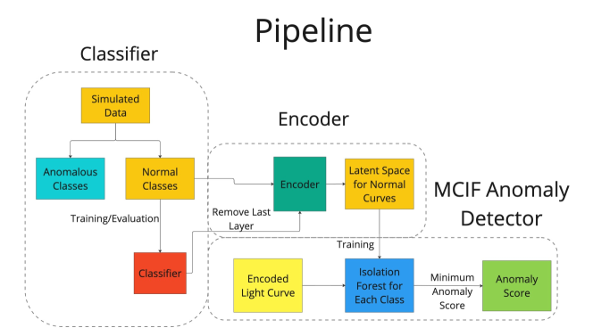
Figure 1: A visual summary of the architecture described in this work. Our approach first trains a classifier, then repurposes it as an encoder, and finally applies Multi-Class Isolation Forests (MCIF), proposed in this work, for anomaly detection.

Figure 1 summarizes our methodology. First, we train a Recurrent Neural Network (RNN) to classify the common classes of transients. Then, we remove the final layer of the trained model and use the remaining architecture as an encoder. We restricted the penultimate layer of the classifier, the output of our encoder, to have 9 neurons during training. To effectively extract anomalies from a well-represented space, it is essential to ensure that transients from similar classes cluster together. In our encoder, the latent space is directly used for light curve classifications, which should naturally lead to clustering of similar transients.

Once we have established this representation space, we must extract anomalies from it. However, when dealing with multiple clusters, a single isolation forest may struggle to capture each cluster equally (for further details, refer to Appendix A). This challenge motivated our approach, MCIF, where we train an isolation forest for each class, representing a distinct cluster, and select the minimum anomaly score as the final score. This minimum score should come from the cluster to which the latent observation is closest, providing the desired functionality.

3.2 Classifier

We train a DNN (Deep Neural Network) classifier that maps a matrix of multi-passband light-curve data $\bm{X}_{s}$ for a transient $s$ to a $1\times N_{c}$ vector of probabilities, reflecting the likelihood of the given light curve being each of the aforementioned non-anomalous transient classes, where $N_{c}$ is the number of classes.

The transient classifier utilizes a Recurrent Neural Network (RNN) with Gated Recurrent Units (GRU, Cho et al., 2014) to handle the sequential time series data. The input for each transient, $\bm{X}_{s}$, is a $4\times N_{T}$ matrix where $N_{T}$ is the maximum number of timesteps for any input sample. $N_{T}$ is $656$ in this work, but most transients have much fewer observations. Each row of the input matrix is composed of the following vector,

$$\bm{X}_{sj}=[f_{sj},\epsilon_{sj},t_{sj},\lambda_{p}],$$ (2)

where $f_{sj}$ is the scaled flux for the $j$th observation of transient $s$, $\epsilon_{sj}$ is the corresponding scaled uncertainty, $t_{sj}$ is the scaled time of when the measurement was taken, and $\lambda_{p}$ is the central wavelength of the passband from which the measurement comes from. For the two passbands in ZTF, the central wavelengths used are as follows {$\lambda_{g}=0.4827\mathrm{\mu m}$, $\lambda_{r}=0.6233\mathrm{\mu m}$}. We include flux error to help the DNN model which measurements it can trust more than others to make an accurate classification. To implement the variable length input in tensorflow, we use a Masking layer and pad the arrays with zero entries to make the input matrix as long as the longest light curve (which is of size $N_{T}$).

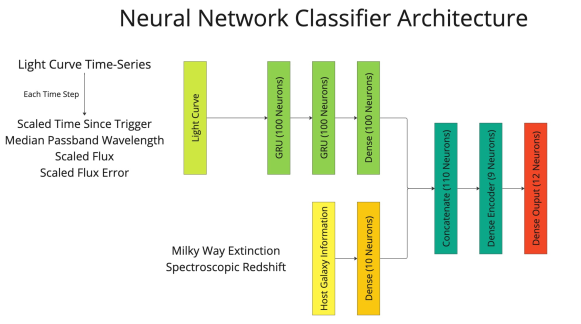
Figure 2: A visualization of the neural network classifier being used in this work. Our model has two input streams, one for real-time light curve data and the other for contextual information. The light curve data (first input stream) goes through multiple GRU layers and then a dense layer. The contextual information (second input stream) feeds through a dense layer. The final dense layers from both input streams are merged into a concatenate layer. We feed that to a nine-neuron dense layer that will serve as the latent space of the encoder. Finally, this dense layer feeds into the output layer which provides classification scores.

This input format has two major advantages. Firstly, it eliminates the need for interpolation methods to pass sequential data into our model. Interpolation or imputation is often needed in astronomical transient classifiers as observations are recorded at irregular intervals. For real-time light curve tasks, linear interpolation is sometimes used (e.g. Muthukrishna et al., 2022) but yields poor results for sparse light curves or surveys with larger cadences, such as LSST. Linear interpolation may confuse models, particularly when applied to a light curve with prolonged intervals of missing data. In such cases, extended sequences of the interpolated light curve may represent only two original observations.

Gaussian Processes (GP) interpolation has shown success for light curve data (e.g. Boone, 2019 and Villar et al., 2021) but does not help with real-time anomaly detection as it requires the whole light curve to perform the interpolation. Villar et al. (2021) gives justification for using GP for real-time anomaly detection, stating that each new observation heavily anchors the GP and that the GP is similar to physical model priors. However, not having access to full light curve information while making real-time predictions is better suited.

The second advantage of our input method is the inclusion of wavelength information to represent different passbands. Previous works have typically passed the light curves from different passbands separately, resulting in even larger sequences of missing (thus interpolated or imputed) data in the common case where some passbands have significantly fewer observations than other passbands. In our work, the inclusion of the central wavelength helps the model learn the relationship between different passbands, infer parts of the light curve in bands where few observations are present, and allows for all data to be passed in one channel.

From ZTF, we only get data in the $g$ and $r$ passbands which makes the difference in passbands less significant. However, the upcoming Vera Rubin Observatory and other large-scale transient surveys will have data in up to six different passbands, and giving the model insight into relationships between different passbands will be crucial. This learned relationship, along with some transfer learning, may make it possible to consolidate data from multiple observatories with different passbands to train one model or allow for a model trained on data from one observatory to be quickly used on data from another observatory.

After the recurrent layers of the DNN, we pass some contextual information into the classifier, which has been shown to be helpful for light curve classification (Foley & Mandel, 2013). In this work, we use the Milky Way extinction and the host galaxy’s spectroscopic redshift as additional inputs to the network. However, we understand that spectroscopic redshift is not always available, and future work should include training a model with photometric redshift or without redshift entirely.

Our classifier ultimately takes the form of an encoder with the latent space being the penultimate layer of this network. Because high dimensional latent spaces are hard to cluster, we deliberately set this layer to have nine neurons. However, the nine-neuron layer may serve as a large bottleneck for the network, forcing it to learn to encode light curves to a space smaller than required for accurate classification. While fine-tuning the size of this layer could help with classification, we would risk giving the isolation forest too many irrelevant features without knowing of doing so until final evaluation (see §3.4).

One of the advantages of using a neural network-based architecture over hand-selected features is that it is a data-driven model, which should make it more sensitive to identifying out-of-distribution data. This inherent quality of neural networks makes them especially good for anomaly detection.

Figure 2 illustrates the architecture of the neural network classifier. The classifier was implemented using keras and tensorflow (Chollet, 2015). We detail the activation functions used in each layer of our classifier as follows. The input stream that each layer is part of is shown in parentheses.

1. Input Layer 1 (Light Curve Stream) - Takes a matrix of shape $4$ x $N_{T}$ as input to the Recurrent Neural Network.

2. Gated Recurrent Unit (Cho et al., 2014) (Light Curve Stream) - Two recurrent layers consisting of 100 gated recurrent units with tanh activation functions.

3. Dense (Light Curve Stream) - A dense layer consisting of 100 neurons with tanh activation functions.

4. Input Layer 2 (Contextual Stream) - Takes a vector of length $2$ containing the Milky Way extinction and spectroscopic redshift.

5. Dense (Contextual Stream) - A dense layer consisting of 10 neurons with ReLU activation functions. This dense layer is connected to Input Layer 2.

6. Concatenate Layer - A layer to merge the 2 streams of input. This layer concatenates the final dense layers for each input stream into one layer with 110 neurons.

7. Dense - A layer with nine neurons to act as the latent representation for the light curves with a ReLU activation function. This may serve as a bottleneck to the model’s learning.

8. Dense - A layer with 12 neurons (1 for each common transient class). This layer has a softmax activation function to map the output values to a probability score.

In our final model architecture, we use GRU layers (Gated Recurrent Units) proposed and tested in Cho et al. (2014). They are shown to perform better than typical Recurrent Neural Networks (RNNs) and have quicker training times than LSTMs (Chung et al., 2014).

To counteract imbalances in the distribution of classes in the dataset, we use a weighted categorical cross-entropy as a loss function with the weight $w_{c}$ proportional to the fraction of transients from each class $c$ in the training set,

$$w_{c}=\frac{N}{N_{c}}$$ (3)

where $N_{c}$ is the number of transients from the class $c$ and $N$ is the total number of samples in the training set. This weighting scheme ensures that classes with fewer samples have higher weights. To train the classifier, we ran it over $40$ epochs using the Adam optimizer (Kingma & Ba, 2017) with EarlyStopping implemented in keras.

3.3 Multi-Class Isolation Forests

Once the classifier is trained, we remove the last layer and use the remaining architecture to map any light curve to the latent space. We define this encoder as a function $E(\bm{X}_{s})$, that takes the aforementioned preprocessed light curve data, $\bm{X}_{s}$, and maps it to a 9-dimensional latent space $\bm{z}_{s}$,

$$\bm{z}_{s}=E(\bm{X}_{s})$$ (4)

For anomaly detection, we now want to compute the anomaly score,

$$a_{s}=A(\bm{z}_{s}),$$ (5)

where $A(\bm{z}_{s})$ is a function that evaluates the anomaly score $a_{s}$ for a latent observation $\bm{z}_{s}$. The goal of this work is to generate relatively large anomaly scores for anomalous transients and smaller anomaly scores for non-anomalous transients.

Isolation Forests are known to be a very simple yet effective anomaly detection algorithm, especially in the domain of astronomical time series. However, using a single isolation forest performs poorly in determining some common classes as non-anomalous. This challenge arises from the complexity of our latent space, which contains various distinct clusters that pose difficulties for a single isolation forest to differentiate. Thus, we propose a new framework where an isolation forest is trained separately on data from every class, using the minimum anomaly score from any isolation forest as the final anomaly score. We call this approach Multi-Class Isolation Forests (MCIF).

We define $12$ isolation forests, $I_{c}(\bm{z}_{s})$, trained on latent space observations from the common transient class $c$. The final anomaly score is defined as

$$A(\bm{z}_{s})=\min_{\forall c}\Bigl{(}-I_{c}(\bm{z}_{s})\Bigr{)}$$ (6)

The function $I_{c}(\bm{z}_{s})$ is positive for less anomalous transients and negative for anomalous ones, to be consistent with the sklearn implementation of Isolation Forests. We negate the scores as we prefer defining transients with higher anomaly scores to be more anomalous, but this makes no difference to the results. All isolation forests used in this work are trained with 200 estimators. The results of using a single isolation forest and the benefits of using Multi-Class Isolation Forests (MCIF) are explored further in Appendix A.

3.4 Limitations of Evaluating Anomaly Detection Methods

Evaluating the performance of anomaly detection models is challenging because anomalies are rare, and it is difficult to build validation sets that account for the unknown. To simulate seeing anomalous data for the first time, the five aforementioned anomalous classes are not revealed to the model until final evaluation. This approach mimics the real-world situation where anomaly detectors (and astronomers) have limited knowledge of the anomalies they may discover.

The goal of this work is not to identify the specific anomalous classes mentioned, but rather to detect anomalies in general. Hence, using physical model priors or giving the model any information about anomalous classes beforehand would reveal too much about the specific rare transient classes used in this work. This could hinder the model’s performance on novel, real-world anomalies that may differ from the ones used in this study.

4 Results and Analysis

In this section, we first evaluate the performance of our neural network classifier on distinguishing between common transient classes (§4.1). We then analyze how well our proposed anomaly detection pipeline, utilizing the classifier as an encoder (§4.2), is able to identify rare/anomalous transients (§4.3). We trained the classifier on simulated light curves from 12 common transient classes that match the ZTF observing conditions and population distributions. We repurposed the trained classifier as an encoder by removing the output layer. The penultimate layer of this encoder, with only 9 neurons, serves as a latent representation of the input light curves. We applied our novel Multi-Class Isolation Forest (MCIF) anomaly detection method to this latent representation. MCIF was trained on latent representations of the common classes to model the known transient population. To evaluate its performance, we tested our approach on latent representations derived from light curves of 5 rare transient classes unseen during training. By construction, the classifier’s latent space should cluster together light curves belonging to similar transient classes, aiding anomaly detection.

4.1 Classifier

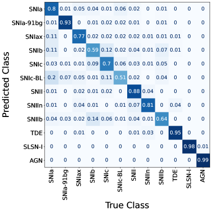
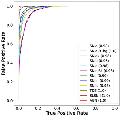
Figure 3: The normalized confusion matrix [left] and ROC curve [right] of the 12 common transient classes used for training given full light curve data. Each cell in the confusion matrix signifies the fraction of transients from each True Class that was classified into the Predicted Class. The ROC curve illustrates the True Positive Rate against the False Positive Rate across various threshold probabilities for each class, with the Area Under ROC curve (AUROC) in parenthesis. The model’s evaluation is conducted on the test set consisting of 10% of the data from the common classes and all anomalous data.

In this section, we evaluate the performance of our classifier which was trained on 80% of the data from the 12 common transient classes. The remaining 20% was split equally into a validation set and a test set used for the final evaluation of the classifier.

The normalized confusion matrix in Figure 3 [left] illustrates the classifier’s ability to accurately predict the correct transient class on the test data. Each cell indicates the fraction of transients from the true class that are classified into the predicted class. The high values along the diagonal, approaching 1.0, indicate strong performance. The misclassifications, indicated by the off-diagonal values, predominantly occur between subclasses of Type Ia supernovae (SNIa, SNIa-91bg and SNIax) and between the core-collapse supernova types (SNIb, SNIc, SNII subtypes), which is expected given their observational similarities. These SNe have been shown to confuse previous models (see Fig. 7 of Muthukrishna et al., 2019).

While the confusion matrix provides valuable insights into the accuracy of our model, it only considers the highest-scoring predicted class and does not use the continuous probability scores that our classifier outputs for each possible class. The Receiver Operating Characteristic (ROC) curve, shown in Figure 3 [right], effectively uses these probabilities. It plots the True Positive Rate (the fraction of positive samples correctly identified as positive) against the False Positive Rate (the fraction of negative samples incorrectly identified as positive) for each class across a range of threshold probability values. This metric is particularly useful in a multi-class context, as it captures the model’s ability to assign low probabilities to several classes when it is uncertain. A key measure of performance, the Area Under the ROC Curve (AUROC), quantifies the overall ability of the classifier to discriminate between classes. In our study, high AUROC values, approaching 1 for all classes, underscore the robustness of our classifier.

A brief comparison of the results in this work and those of a similar DNN light-curve classifier (RAPID; Muthukrishna et al., 2019) hints that our classifier can perform on par with a reasonable baseline and has better accuracies for many classes. This improvement can be attributed, in part, to the use of an improved simulated dataset that has fixed some known problems with core-collapse supernovae. RAPID also included some of the rare classes that we deliberately did not include in our classifier and instead designated as anomalous (See Fig. 7 of Muthukrishna et al., 2019). While our classification methodology was very similar to RAPID, a key difference was our unique input method that bypassed the missing data problem. Future work should compare the effectiveness of this input method with traditional interpolation or imputation methods, and further comparison is beyond the scope of this work.

4.2 Latent Representation

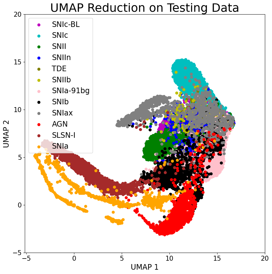
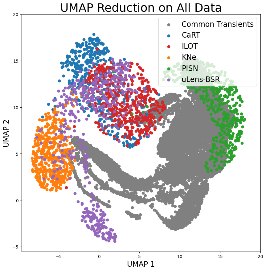
Figure 4: The UMAP reduction of the latent space derived from the test set, which includes 10% of the common transients reserved for testing the classifier [left] and randomly sampled anomalous transients from the unseen anomaly dataset [right]. Despite not being trained on this data, the learned features still exhibit clear visual structure and anomalous transients form distinct clusters separate from the common classes. It is important to note that the UMAP reduction is used only for visualization purposes, and the actual anomaly detection is performed on the nine-dimensional latent space.

After repurposing the classifier as an encoder, we obtain a nine-dimensional latent space. We can visualize this latent space with UMAP (McInnes et al., 2020), a manifold embedding technique, to determine if there is visible clustering. In Figure 4 [left], we plot the UMAP representations of the test data. While it is difficult to examine some of the overlapping classes in this embedded space, there is clear clustering of many of the classes. In Figure 4 [right], we color all of the common classes grey and include a sample of transients from the anomalous classes. We see that the anomalous classes cluster together in the embedded space and separate from the common transients despite the model not being trained on these objects. This level of clustering suggests that our encoder may be discovering generalisable patterns within light curves, and this property may have potential use cases beyond anomaly detection in few-shot classification. It is important to note that we only use UMAP for visualisation purposes and that the latent space used for anomaly detection is obtained directly from the penultimate layer of the classifier.

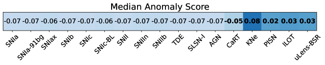
Figure 5: The median anomaly score (rounded to two decimal places) for each class extracted from the latent representations of full light curves. The scores come from the full, unseen anomalous dataset for anomalous classes and the 10% test dataset for common classes. The right 5 classes (in bold) are anomalous. The separation between the scores of anomalous classes and common classes is evident, and the anomaly scores for the common classes are consistently low signifying they are not erroneously marked anomalous.

4.3 Anomaly Detection

After training MCIF on the latent representations of the training data, we pass unseen test data and anomalous data through our pipeline for evaluation. In Figure 5, we list the median anomaly score predicted by MCIF for each class. The anomalous classes have much higher median anomaly scores than the common classes, illustrating a significant distinction between the scores of all common and most anomalous classes. This difference is not as pronounced when using a single isolation forest and the advantages of employing MCIF are discussed further in Appendix A.

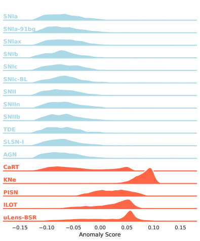
Figure 6: The distribution of anomaly scores for each class, computed using MCIF on the latent representations derived from full light curves. The scores are plotted using $100\%$ of the anomalous dataset (unseen during training) and the test dataset of common classes. The anomalous classes (bottom five in red) generally show higher anomaly scores with positively skewed distributions. The common classes and CaRTs all have low anomaly scores on average.

In Figure 6, we plot the distribution of anomaly scores predicted by MCIF for each class. The plot further demonstrates the distinction in anomaly scores of common and anomalous transients. Notably, there is a significant skew towards larger anomaly scores for the anomalous classes, reaffirming our model’s performance. However, Calcium Rich Transients (CaRTs), despite being one of our anomalous classes, tend to have lower anomaly scores. CaRTs are notoriously difficult to photometrically classify as anomalous due to their resemblance to other common supernova classes (see Fig. 8 of Muthukrishna et al. 2019 for example). One of the most effective ways to detect CaRTs is to observe a calcium line in their spectra, and a robust anomaly detector would use photometric differences to discern this spectroscopic dissimilarity. However, ZTF is limited to only the $g$ and $r$ passbands, which lets this subtle spectroscopic difference go unnoticed. The upcoming Legacy Survey of Space and Time (LSST) on the Rubin Observatory will observe data in six passbands and will likely mitigate this issue.

4.3.1 Anomaly Precision and Recall

To identify anomalies with MCIF, a threshold anomaly score would need to be chosen such that the common transient classes are not flagged as anomalous, but the anomalous classes are flagged as anomalous. This threshold score needs to lead to a high precision and a high recall of anomalies. Precision is a measure of how pure our anomaly predictions are, and recall is a measure of how many anomalies we can expect to find. We define anomaly precision and recall as

$$P_{c,\tau}=\frac{|\{L^{s}\in L^{c}\mid A(L^{s})>\tau\}|}{|\{L^{s}\in L\mid A(L^{s})>\tau\}|}$$ (7)

$$R_{c,\tau}=\frac{|\{L^{s}\in L^{c}\mid A(L^{s})>\tau\}|}{|L^{c}|}$$ (8)

where $P_{c,\tau}$ and $R_{c,\tau}$ are the precision and recall of class $c$, the tested class, at threshold anomaly score $\tau$, $L^{c}$ is the set of all transients from class $c$ in $L$, and $L$ is the set of all transients. We further define the set $L$ to be comprised of half class $c$ and half of transients coming from the opposite type as $c$ when computing the precision and recall for class $c$. For example, if the tested class was KNe, the set $L$ would contain half KNe and half common transients. Note that only precision is influenced by the composition of $L$.

In other words, precision is calculated as the number of predicted anomalies from each class divided by the total number of predicted anomalies, and recall is calculated as the number of predicted anomalies from each class divided by the total number of transients of that class. Both are defined given a threshold anomaly score and over a deliberately defined sample (as described above).

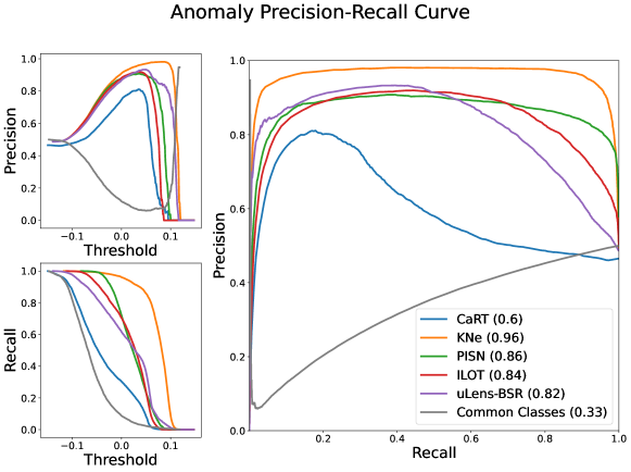
Figure 7: The precision-recall curves for our anomaly detection pipeline for each anomalous class and a grey line indicating the average across all common classes. The precision and recall are plotted against the threshold anomaly score in the left sub-figures. Precision and recall are defined in Equation 7 and Equation 8, respectively, and calculated on a set comprising half of the transients from the tested anomalous class and half randomly sampled common transients (all coming from the test data that was unseen by the model). Promisingly, the Area Under the Precision-Recall Curve (AUCPR) for each anomalous class (except CaRTs) is very high. The AUCPR for the common classes is low indicating that they are not often predicted as anomalous by MCIF.

In Figure 7 we plot the anomaly precision and recall at various threshold anomaly scores $\tau$ for all anomalous classes and an average for all common classes. In this context, the precision is $0.5$ at the lowest threshold, as at that point all transients are marked as anomalous, and 50% of them are from the tested class. Recall is $1$ at the lowest threshold, much like for many other machine learning tasks, as all transients of the tested class are identified as anomalous. This interpretation serves as the rationale for the 50-50 composition of the set $L$, as otherwise, it would be difficult to standardize AUC scores across anomalous and common classes.

The Area Under the Precision-Recall Curve (AUCPR) is a good indicator of how often a class is being marked anomalous. The AUCPR scores for anomalous classes are significantly better than the AUCPR scores for the common classes, even CaRTs. However, the precision of the common classes jumps suddenly at high thresholds while it declines for anomalous classes. This signifies that the transients with the highest anomaly scores are false positive anomalies. This phenomenon is understandable if we consider that most anomalies populate anomaly scores $a_{s}\lesssim 0.1$ in Figure 6. Beyond this, at thresholds $\tau\gtrsim 0.1$, the recall drops as these anomalous transients no longer meet the threshold. With inherently more common transients, a few extreme latents among them dictate precision initially. Figure 8 confirms that the top 5-10 candidates are common transients, but after this, as $\tau$ reduces, our model captures a much higher fraction of true anomalies.

Selecting a threshold anomaly score near the inflection point on the top right of the precision-recall curve will be a good choice for identifying as many anomalies as possible while still having a pure sample with few false positives.

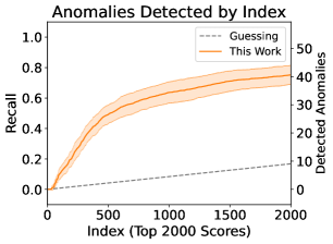
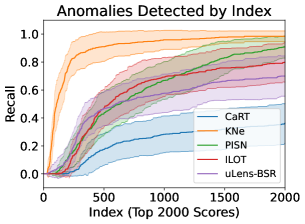
Figure 8: Anomalies detected in the 2,000 top-ranked transients by MCIF anomaly score index, using a test sample reflecting the estimated frequency of anomalies in nature. In the sample of 12,040 common transients and 54 anomalous transients, the model recalls $41\pm 2$ $(\sim 75\%)$ of the anomalies after following up the top 2000 ranked transients. The left plot aggregates all anomalies and the right plot delineates per class. To control for the variance imposed by the small anomaly sample size, we repeat the sampling 50 times. The mean and standard deviation of detected anomalies are plotted as the solid lines and shaded regions, respectively.

4.3.2 Detection Rates in a Representative Population

The previous results do not take into account that anomalous transients are inherently less frequent than common transients. While the frequency of anomalies in nature is not known, a good estimate for the expected population frequency was presented in Kessler et al. (2019a) for the PLAsTiCC dataset (The PLAsTiCC team et al., 2018). The rate of common transients, as defined in this work, was roughly 220 times larger than that of anomalous transients, using PLAsTiCC frequencies for each class. We used this rate to randomly select a more realistic test dataset that contained 12,040 normal transients and 54 anomalies. Randomly selecting a representative sample of only 54 anomalies is subject to significant variance. Therefore, we created 50 sample datasets to perform 50-fold cross-validation. The mean and standard deviation of the number of transients from each class present in our 50 test samples are listed in Table 1.

For each validation set, we ranked the transients by the anomaly scores predicted by MCIF. We followed up the top 2000 ranked transients (roughly 15% of the dataset) as the candidate pool. Across 50 repeated trials, we identified $41\pm 2$ out of the 54 true anomalies in our dataset (recalling $\sim 75\%$ of the anomalies). In Figure 8, we plot the fraction of anomalies recalled and the total number of anomalies recovered for thresholds up to the top 2000 transients. MCIF recalls most anomalies within candidates having the highest anomaly scores, followed by a tapering as fewer anomalies remain.

Examining the detection rate for each anomaly class, we see that the model’s trouble in identifying CaRTs as anomalous brings down the overall anomaly recall. This plot and the precision-recall curves show a consistent pseudo-hierarchy of which anomalies are easiest to detect. If we exclude CARTs from our sample of anomalies, our recall of anomalies increases to $47\pm 2$ out of the 54 true anomalies in our dataset (recalling $\sim 87\%$ of the anomalies).

It’s worth emphasizing that the objective of this work is to identify anomalies in a general sense rather than tailoring to specific classes, and therefore, this work does not rely on specific information about the anomalous classes defined (see §3.4). The only specific attribute used is the estimated frequency of anomalies (220 times less frequent than the common classes), which serves as a reference as it’s impossible to estimate a similar number for anomalies that have never been observed.

4.3.3 Real-Time Detection

Identifying anomalies in real-time is important for obtaining early-time follow-up observations, which is crucial for understanding their physical mechanisms and progenitor systems. However, directly assessing our architecture’s real-time performance is challenging due to the irregular sampling of light curves in our input format.

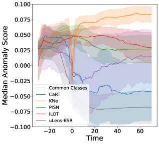
Figure 9: Median MCIF anomaly score over time for a sample of transients from the test set. Real-time anomaly scores are calculated at intervals of 1 day for a sample of 2000 common and 2000 total anomalous light curves. The left plot shows the scores for the common and anomalous transients as a whole, while the right plot shows each anomalous class individually. The anomaly scores for the common transients decline before the trigger, while the anomalous transients remain at high scores throughout most of the transient’s evolution.

To assess the real-time performance of our architecture, we plot the median anomaly scores over time for a sample of 2000 common and 2000 anomalous transients in Figure 9. To construct this plot without relying on interpolation, we calculate scores at discrete times $l$ sampled at 1-day intervals from $-30$ to $70$ days relative to trigger, using only observations occurring before each time $l$ to mimic a real-time scenario. To ensure sufficient information for robust scoring, we only consider transients where the final observation was recorded after time $l-5$. The results show a clear divergence where common transient scores tend to decline around trigger, while anomalous transient scores remain consistently high.

Figure 9 reveals two notable irregularities. Firstly, the anomaly scores for common transients decline before trigger, which is unexpected given that the pre-trigger phase of most transient classes should primarily consist of background noise. Further analysis of the pre-trigger classification results (Figure 13) reveals that certain transients, most notably SLSN-I and AGN, are almost all classified before trigger, thereby lowering the average anomaly score for common transients. This can be attributed to the fact that redshift and pre-trigger information such as host galaxy color and some AGN pre-trigger variability are particularly useful for classifying these transients before trigger (see Figure 16 of Muthukrishna et al., 2019).

Secondly, KNe exhibit a significant dip around the time of trigger. Upon further analysis, we found that certain common transient classes also experienced a similar dip around trigger; however, unlike KNe, they do not rebound back to higher anomaly scores. This dip is related to the inherent nature of the trigger of a light curve, which often marks the first real observation of the transient phase of a light curve, and serves as a reset for the anomaly score. A more detailed analysis of this phenomenon is provided in Appendix B.

These preliminary findings suggest the potential for enabling real-time identification of anomalous transients. While some known rare classes can be difficult to distinguish from the common classes without a significant amount of data, others can be detected surprisingly soon after trigger. The ability to flag unusual events early in their evolution could prove invaluable for optimizing the allocation of follow-up resources and maximizing the scientific returns from rare transient discoveries.

5 Conclusion

The advent of large-scale wide-field surveys has revolutionized time-domain astronomy, unveiling an extraordinary diversity of astrophysical phenomena. Surveys such as the Zwicky Transient Facility (ZTF) and the upcoming Legacy Survey of Space and Time (LSST) conducted by the Vera C. Rubin Observatory promise to discover transients in vast numbers, with LSST expected to generate millions of alerts each night. This deluge of data presents both a challenge and an opportunity: while the sheer volume of detections makes manual inspection infeasible, it also offers the potential to discover entirely new classes of transients that are rare or have remained hidden in previous surveys. To fully harness the potential of these wide-field surveys, automated methods for real-time anomaly detection are essential. By identifying and prioritizing the most unusual and interesting events amid the flood of data, these techniques can facilitate rapid follow-up and characterization, enabling us to deepen our understanding of the time-domain universe.

The most common approach for transient anomaly detection is to construct a feature extractor that can map light curves to a low-dimensional latent space, and then apply clustering or outlier detection algorithms to identify anomalies within that space. Constructing a latent space that represents transients well for anomaly detection is difficult, and most previous approaches have either user-defined features or unsupervised deep-learning approaches.

In this work, we have introduced a novel approach that leverages the latent space of a neural network classifier for identifying anomalous transients. Our pipeline, which combines a deep recurrent neural network classifier with our novel Multi-Class Isolation Forest (MCIF) anomaly detection method, demonstrates promising performance on simulated data matched to the characteristics of the Zwicky Transient Facility.

The key advantages of our approach are:

1. The recurrent neural network (RNN) classifier maps light curves into a low-dimensional latent space that naturally clusters similar transient classes together, providing an effective representation for anomaly detection. We repurposed the penultimate layer of this classifier as the feature space for anomaly detection.

2. Our novel MCIF method addresses the limitations of using a single isolation forest on the complex latent space by training separate isolation forests for each known transient class and taking the minimum score as the final anomaly score.

3. Our classifier input format eliminates the need for interpolation by incorporating time and passband information, enabling the model to learn inter-passband relationships and handle irregular sampling.

To mimic a real-world scenario, we evaluated our approach on a realistic simulated dataset containing 12,040 common transients and 54 anomalous events. After following up MCIF’s top 2000 ranked transients, we accurately identified $41\pm 3$ out of the 54 true anomalies. That is, after following up the top 15% highest ranked scores, we recovered 75% of the true anomalies. CARTs look very similar to common supernovae, and thus are difficult to identify. If we exclude CARTs from our anomalous sample, our recovery of anomalies increases sharply to $85\%$ ($46\pm 2$ out of the 54 true anomalies) after following up the top 2000 ($\sim 15\%$) highest-scoring transients.

The learned latent space exhibits clear separation between common and anomalous transient classes, and our preliminary analysis suggests the potential for real-time anomaly detection using limited early-time observations. The pre-trigger information encoded by our RNN enables our model to identify anomalous transients at early stages in the light curve, and even by trigger, a significant separation between common and anomalous transients is captured. In particular, KNe, PISN, and ILOTs all stand out as anomalous shortly after the time of trigger.

Future work encompasses several promising directions. Firstly, benchmarking our model against other similar approaches is important for a comprehensive performance assessment. Currently, comparing models is difficult, because a standard test dataset of anomalies does not exist. Developing a realistic benchmark dataset that encompasses a representative population of common and example anomalous transients will improve the quality of methods developed by the community and enable robust evaluation metrics. Moreover, a detailed comparative analysis of MCIF with previous class-by-class anomaly detection approaches should be carried out to gain a deeper understanding of their relative strengths and limitations in this domain.

Secondly, integrating techniques from other anomaly detection methods, such as active learning (Lochner & Bassett, 2021), could help to distinguish new anomalies as interesting or not. Beyond direct anomaly detection, MCIF can be used to identify which known class an anomalous object most closely resembles based on the individual Isolation Forest scores. Additionally, we plan to apply the proposed architecture to real observational data, moving beyond simulations and testing the model’s effectiveness in a practical astronomical context.

A significant contribution of this work is the demonstration that a well-trained classifier can be effectively repurposed for anomaly detection by leveraging the clustering properties of its latent space. The flexibility of our approach allows for the adaptation of any classifier to an anomaly detector. For example, using existing classifiers as feature extractors for spectra, images, or time series from other domains, we can build effective anomaly detectors.

Another significant advantage of our approach is that the clustering properties of the latent space extend to unseen data, enabling few-shot classification of astronomical transients with limited labeled examples. This will be useful for the early observations from new surveys such as LSST. Furthermore, our input method lends itself well to transfer learning from one survey to another because it explicitly uses the passband wavelength. Future work should explore transfer learning from ZTF data to other surveys such as PanSTARRS or LSST simulations.

In conclusion, our novel approach to real-time anomaly detection in astronomical light curves, combining a deep neural network classifier with Multi-Class Isolation Forests, demonstrates the power of leveraging well-clustered latent space representations for identifying rare and unusual transients. As the era of large-scale astronomical surveys continues to produce unprecedented volumes of data, the development and refinement of such techniques will be crucial for making discoveries in time-domain astronomy.

Data Availability

The models used to create the simulations that generate the data used in this work were released in PLAsTiCC (Kessler et al., 2019b) and are available at https://zenodo.org/record/2612896#.YYAz1NbMJhE. To generate light curves following ZTF observing properties, we use the SNANA software package (Kessler et al., 2009), developed for PLAsTiCC, with observing logs from the ZTF survey to generate data. A version of these simulations was first used in (Muthukrishna et al., 2019) and have since been updated to resolve a known problem with core-collapse SNe. The data is publicly available upon reasonable request to the corresponding author.

Appendix A Advantages of MCIF

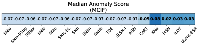
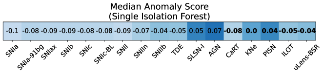
Figure 10: The median anomaly score for each class computed for latent representations of transients obtained from full light curves when a single isolation forest is used for anomaly detection [bottom] and when MCIF is used [top] (this is the exact same as Figure 5, reproduced for convenience). The scores are derived from the unseen anomalous data and the common transient testing data. The right 5 classes (scores in bold) are anomalous. The common classes have somewhat lower median scores when using a single isolation forest, but the common classes SLSN-I and AGN (among others) are considered very anomalous, unlike when using MCIF.

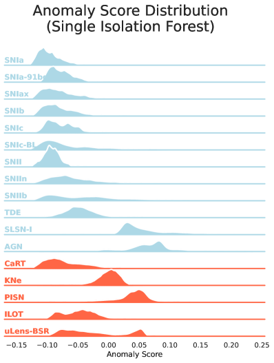
Figure 11: The distribution of anomaly scores for full light curves when using a single isolation forest for anomaly detection. The scores are derived from the unseen anomalous data and the common transient testing data. The bottom 5 classes (in red) are the anomalous classes. There is some separation between the anomaly scores of common and anomalous classes, but certain common classes are considered very anomalous.

Before proposing the MCIF pipeline, we attempted to use a normal isolation forest to detect anomalies from the latent representation $z_{s}$ of a light curve. We trained an isolation forest on all the common classes of our training data using $200$ estimators. To account for the class imbalance in our training data, we weighted samples from underrepresented classes more heavily during the training of the isolation forest, using the same weighting scheme as in Equation 3. The anomaly score function $A(Z_{s})$ was simply the negated anomaly score output from a single isolation forest trained on all the latent representations of the training data.

As shown in Figure 10, there is little distinction in the anomaly scores of most anomalous and common classes when using a single isolation forest. Surprisingly, the common classes SLSN-I and AGN are classified as relatively more anomalous than all the other classes. The distribution of anomaly scores in Figure 11 reveals that although there is overall separation between common and anomalous classes, certain common classes are classified as very anomalous.

The UMAP reduction of the latent space, as depicted in Figure 4, provides insight into this behaviour. The SLSN-I and AGN classes are significantly distant from the main cluster formed by other classes. This isolation from the central cluster may explain the high anomaly scores associated with these classes. This hypothesis is also supported by the near-perfect classification of these classes, shown in the confusion matrix and ROC curves in Figure 3. In fact, the near-perfect classification hinted towards this poor result in anomaly detection, showing us that these transients are easy to separate from other classes, and hence are also easy to mark anomalous. In summary, while an isolation forest is good at detecting anomalies, it struggles to capture the structure of a latent space with numerous clusters. This drawback of using a single isolation forest could explain why other works report high anomaly scores for SLSN-I and AGN. Using a class-by-class (or cluster-by-cluster) anomaly detector, such as MCIF, can mitigate this. Directly comparing Figure 6 and Figure 11 empirically demonstrates the advantages of MCIF.

Appendix B The Kilonova Dip

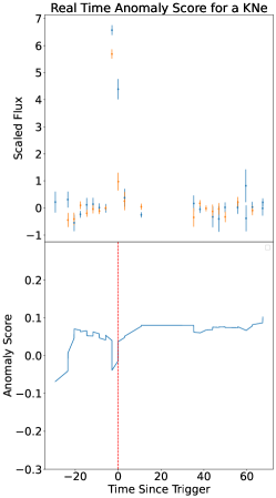
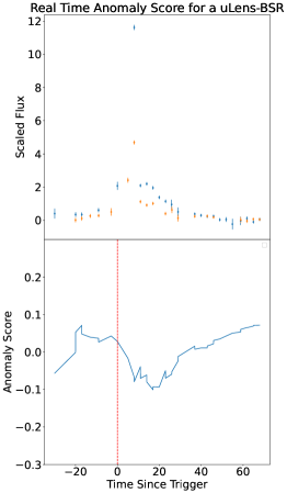
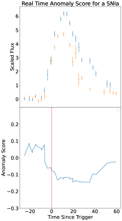
Figure 12: Real-time anomaly scores for a sample KN, uLens-BSR, and SNIa. They all exhibit a significant dip near trigger, but the dip for the SNIa is followed by a further decline, whereas KNe and uLens-BSR show a sharp increase after the dip.

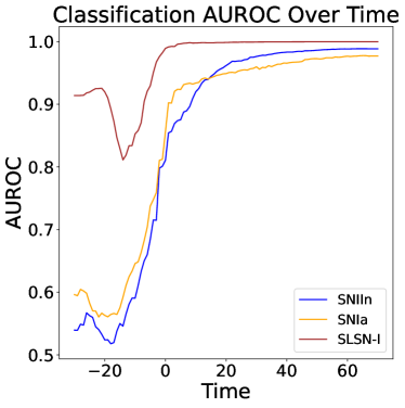
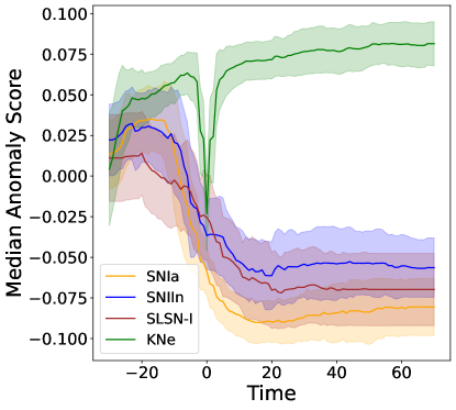
Figure 13: Real-time AUROC values for selected classes [left] and real-time anomaly scores for a different subset of classes than Figure 9 [right]. Classes that are poorly classified pre-trigger (e.g. SNIIn, and SNIa) exhibit a dip in anomaly score similar to KNe, which coincides precisely with the sudden increase in classification accuracy.

As illustrated in Figure 9, there is an unusual dip in the anomaly scores of KNe around the trigger time. Further analysis reveals that most common classes also experience a similar dip at trigger, but they do not rebound to high anomaly scores afterward. Examples are shown in Figure 12.

The trigger of a light curve often corresponds to the first observation detected as part of the transient phase of the light curve, and very few common classes can be effectively classified before trigger. Effective pre-trigger classification is likely due to host galaxy information (host redshift and Milky Way extinction) or the periodic nature of certain transient events (e.g. AGNs) which means they are midway through their evolution at trigger. Figure 13, shows that classes with a high pre-trigger classification accuracy (e.g. SLSN-I) have consistently declining anomaly scores before trigger. In contrast, classes with poor pre-trigger classification (e.g. SNIIn and SNIa) exhibit a slight increase in anomaly scores before trigger, followed by a sudden dip. This sudden dip resembles the behaviour of KNe and coincides perfectly with the sudden jump in classification performance. This suggests that our pipeline struggles to detect KNe as anomalous before trigger for the same reasons it is unable to classify SNIIn before trigger. Despite KNe exhibiting a slight upward trend before trigger, it seems that the new observation near trigger means much more (likely due to the high S/N of that observation).

For observations after trigger, we found that the anomaly score “resets” to mark the true beginning of the transient phase. For example, in the case of KNe, the high S/N trigger observation signals the actual start of the transient and resets the anomaly score. Subsequent observations, characterised by a sudden decline back to the background level, quickly push KNe into the anomalous category (as short-time-scale events are rare). However, in the case of poorly classified common classes, this reset is followed by a further decline in anomaly score as classification accuracy increases, making the dip appear normal. A similar effect can be seen in other anomalous classes, most notably in uLens-BSR transients. The result is less pronounced as the first rise of uLens-BSR transients does not always coincide with trigger, leading to a distributed dip around trigger for uLens-BSR in Figure 9 and a dip offset from trigger in Figure 12.

Appendix C Example Light Curves

A sample light curve from each class is illustrated in Figure 14.

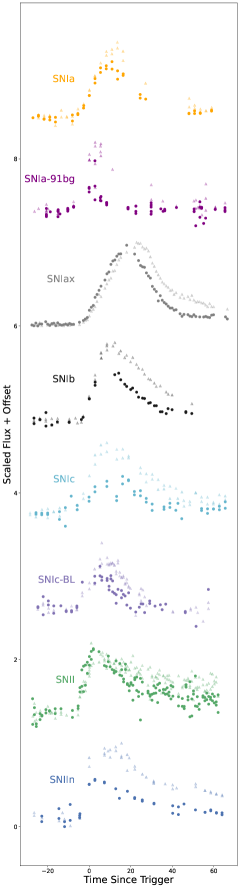
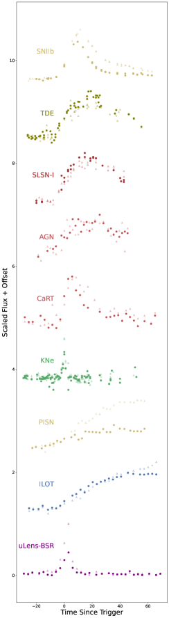
Figure 14: Sample light curves from each transient class used in this work. We only plot transients with low signal-to-noise and low host redshift ($z<0.5$) to help visually compare shapes. The dark circular markers represent the r band while the light triangular markers represent the g band. Flux errors are not plotted.

References

- Abadi et al. (2015) Abadi M., et al., 2015, TensorFlow: Large-Scale Machine Learning on Heterogeneous Systems, https://www.tensorflow.org/
- Abbott et al. (2017) Abbott B. P., et al., 2017, Physical Review Letters, 119, 161101
- Astropy Collaboration et al. (2022) Astropy Collaboration et al., 2022, ApJ, 935, 167
- Bellm et al. (2018) Bellm E. C., et al., 2018, Publications of the Astronomical Society of the Pacific, 131, 018002
- Bi et al. (2018) Bi J., Feng T., Yuan H., 2018, Computers in Industry, 97, 76
- Boone (2019) Boone K., 2019, The Astronomical Journal, 158, 257
- Charnock & Moss (2017a) Charnock T., Moss A., 2017a, ApJ, 837, L28
- Charnock & Moss (2017b) Charnock T., Moss A., 2017b, The Astrophysical Journal, 837, L28
- Cho et al. (2014) Cho K., van Merrienboer B., Gulcehre C., Bahdanau D., Bougares F., Schwenk H., Bengio Y., 2014, in Proceedings of the 2014 Conference on Empirical Methods in Natural Language Processing (EMNLP). Association for Computational Linguistics, pp 1724–1734, doi:10.3115/v1/D14-1179
- Chollet (2015) Chollet F., 2015, keras, https://github.com/fchollet/keras
- Chung et al. (2014) Chung J., Gulcehre C., Cho K., Bengio Y., 2014, in NIPS 2014 Workshop on Deep Learning, December 2014.
- Coppejans et al. (2020) Coppejans D. L., et al., 2020, ApJ, 895, L23
- Etsebeth et al. (2023) Etsebeth V., Lochner M., Walmsley M., Grespan M., 2023, Astronomaly at Scale: Searching for Anomalies Amongst 4 Million Galaxies (arXiv:2309.08660)
- Feng et al. (2017) Feng T., Du Z., Sun Y., Wei J., Bi J., Liu J., 2017, in 2017 IEEE International Congress on Big Data (BigData Congress). pp 224–231, doi:10.1109/BigDataCongress.2017.38
- Foley & Mandel (2013) Foley R. J., Mandel K., 2013, The Astrophysical Journal, 778, 167
- Giles & Walkowicz (2019) Giles D., Walkowicz L., 2019, MNRAS, 484, 834
- Harris et al. (2020) Harris C. R., et al., 2020, Nature, 585, 357
- Hunter (2007) Hunter J. D., 2007, Computing in Science & Engineering, 9, 90
- Ishida et al. (2021) Ishida E. E. O., et al., 2021, A&A, 650, A195
- Ivezić et al. (2019) Ivezić Ž., et al., 2019, ApJ, 873, 111
- Kasen (2010) Kasen D., 2010, ApJ, 708, 1025
- Kessler et al. (2009) Kessler R., et al., 2009, Publications of the Astronomical Society of the Pacific, 121, 1028
- Kessler et al. (2019a) Kessler R., et al., 2019a, Publications of the Astronomical Society of the Pacific, 131, 094501
- Kessler et al. (2019b) Kessler R., et al., 2019b, PASP, 131, 094501
- Kingma & Ba (2017) Kingma D. P., Ba J., 2017, Adam: A Method for Stochastic Optimization (arXiv:1412.6980)
- Liu et al. (2008) Liu F. T., Ting K. M., Zhou Z.-H., 2008, in 2008 eighth ieee international conference on data mining. pp 413–422
- Lochner & Bassett (2021) Lochner M., Bassett B. A., 2021, Astronomy and Computing, 36, 100481
- Lochner et al. (2016) Lochner M., McEwen J. D., Peiris H. V., Lahav O., Winter M. K., 2016, ApJS, 225, 31
- Mahabal et al. (2008) Mahabal A., et al., 2008, in AIP Conference Proceedings. AIP, doi:10.1063/1.3059064, https://doi.org/10.1063%2F1.3059064
- Malanchev et al. (2021a) Malanchev K. L., et al., 2021a, MNRAS, 502, 5147
- Malanchev et al. (2021b) Malanchev K. L., et al., 2021b, Monthly Notices of the Royal Astronomical Society, 502, 5147
- McInnes et al. (2020) McInnes L., Healy J., Melville J., 2020, UMAP: Uniform Manifold Approximation and Projection for Dimension Reduction (arXiv:1802.03426)
- McKinney (2010) McKinney W., 2010, in van der Walt S., Millman J., eds, Proceedings of the 9th Python in Science Conference. pp 51 – 56
- Möller & de Boissière (2020) Möller A., de Boissière T., 2020, MNRAS, 491, 4277
- Muthukrishna et al. (2019) Muthukrishna D., Narayan G., Mandel K. S., Biswas R., Hložek R., 2019, Publications of the Astronomical Society of the Pacific, 131, 118002
- Muthukrishna et al. (2022) Muthukrishna D., Mandel K. S., Lochner M., Webb S., Narayan G., 2022, Monthly Notices of the Royal Astronomical Society, 517, 393
- Narayan et al. (2018) Narayan G., et al., 2018, ApJS, 236, 9
- Pasquet et al. (2019) Pasquet J., Pasquet J., Chaumont M., Fouchez D., 2019, A&A, 627, A21
- Pedregosa et al. (2011) Pedregosa F., et al., 2011, Journal of Machine Learning Research, 12, 2825
- Pruzhinskaya et al. (2019a) Pruzhinskaya M. V., Malanchev K. L., Kornilov M. V., Ishida E. E. O., Mondon F., Volnova A. A., Korolev V. S., 2019a, Monthly Notices of the Royal Astronomical Society
- Pruzhinskaya et al. (2019b) Pruzhinskaya M. V., Malanchev K. L., Kornilov M. V., Ishida E. E. O., Mondon F., Volnova A. A., Korolev V. S., 2019b, MNRAS, 489, 3591
- Pérez-Carrasco et al. (2023) Pérez-Carrasco M., et al., 2023, Multi-Class Deep SVDD: Anomaly Detection Approach in Astronomy with Distinct Inlier Categories (arXiv:2308.05011)
- Ricker et al. (2015) Ricker G. R., et al., 2015, Journal of Astronomical Telescopes, Instruments, and Systems, 1, 014003
- Ruff et al. (2018) Ruff L., Vandermeulen R., Goernitz N., Deecke L., Siddiqui S. A., Binder A., Müller E., Kloft M., 2018, in Dy J., Krause A., eds, Proceedings of Machine Learning Research Vol. 80, Proceedings of the 35th International Conference on Machine Learning. PMLR, pp 4393–4402, https://proceedings.mlr.press/v80/ruff18a.html
- Sainburg et al. (2021) Sainburg T., McInnes L., Gentner T. Q., 2021, Parametric UMAP embeddings for representation and semi-supervised learning (arXiv:2009.12981)
- Schölkopf et al. (1999) Schölkopf B., Williamson R. C., Smola A., Shawe-Taylor J., Platt J., 1999, in Solla S., Leen T., Müller K., eds, Proceedings of the 12th International Conference on Neural Information Processing Systems Vol. 12, Advances in Neural Information Processing Systems. MIT Press, https://proceedings.neurips.cc/paper_files/paper/1999/file/8725fb777f25776ffa9076e44fcfd776-Paper.pdf
- Singh et al. (2022) Singh S., Luo M., Li Y., 2022, Multi-Class Anomaly Detection (arXiv:2110.15108)
- Solarz et al. (2017) Solarz A., Bilicki M., Gromadzki M., Pollo A., Durkalec A., Wypych M., 2017, A&A, 606, A39
- Soraisam et al. (2020) Soraisam M. D., et al., 2020, ApJ, 892, 112
- The PLAsTiCC team et al. (2018) The PLAsTiCC team et al., 2018, arXiv e-prints, p. arXiv:1810.00001
- Villar et al. (2021) Villar V. A., Cranmer M., Berger E., Contardo G., Ho S., Hosseinzadeh G., Lin J. Y.-Y., 2021, The Astrophysical Journal Supplement Series, 255, 24
- Walmsley et al. (2022) Walmsley M., et al., 2022, Monthly Notices of the Royal Astronomical Society, 513, 1581
- Waskom (2021) Waskom M. L., 2021, Journal of Open Source Software, 6, 3021
- Webb et al. (2020) Webb S., et al., 2020, MNRAS, 498, 3077