GPolylla: Fully GPU-accelerated polygonal mesh generator

Abstract

This work presents a fully GPU-accelerated algorithm for the polygonal mesh generator known as Polylla. Polylla is a tri-to-polygon mesh generator, which benefits from the half-edge data structure to manage any polygonal shape. The proposed parallel algorithm introduces a novel approach to modify triangulations to get polygonal meshes using the half-edge data structure in parallel on the GPU. By changing the adjacency values of each half-edge, the algorithm accomplish to unlink half-edges that are not used in the new polygonal mesh without the need neither removing nor allocating new memory in the GPU. The experimental results show a speedup, reaching up to $\times 83.2$ when compared to the CPU sequential implementation. Additionally, the speedup is $\times 746.8$ when the cost of copying the data structure from the host device and back is not included.

1 Introduction

Polygonal mesh generation is becoming increasingly important due to the development of new numerical methods, such as the Virtual Element Method (VEM) Vemapplications ; Sorgente2022 . Meshes based on triangles and quadrangles are common in simulations using FEMFEM to solve problems related to heat transfer FEMheattransfer , fluid dynamics FemFluiddunamics and fracture mechanics FEMfracturemechanics , among others. However, FEM elements must obey specific quality criteria KNUPP2003217 , such as having no excessively large obtuse angles or tiny angles, sides of graded length (aspect ratio criterion), and so on. To meet these requirements, it is sometimes necessary to insert a large number of points and elements to model a domain, which can increase the simulation time.

VEM, on the other hand, can use any polygon as a basic cell, improving the simulation speed because of the use of fewer cells than if only triangles and quadrilaterals are used to solve the same problem. Most VEM implementations currently use polygonal meshes formed by Voronoi cells Voronoi , which are convex polygons. Voronoi-based meshes work properly with the VEM but these meshes prevent the researchers or engineers from exploring the full potential of VEM on arbitrary polygonal meshes.

To overcome these limitations, we’ve introduced Polylla, an algorithm designed for generating meshes using arbitrary polygonal shapes. Polylla begins by taking a triangulation as input and then constructs terminal-edge regions by connecting triangles that share a common terminal edge. From these terminal-edge regions, the algorithm creates one or more convex or non-convex polygons whose boundaries are defined by edges that are not the longest edge of any triangle and/or input boundary/interface edges. Figure 1 illustrates a polygonal mesh generated by Polylla.

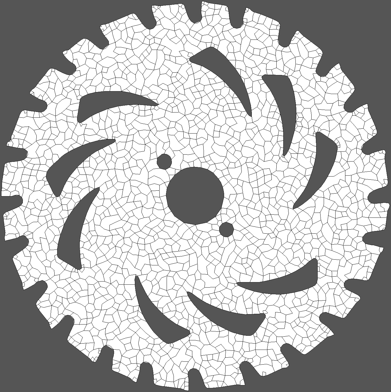
Figure 1: Polygonal mesh of a circular saw generated using Polylla mesh generator.

In general, meshing algorithms can be classified into two groups owen1998survey ; johnen2016indirect : (i) direct algorithms: meshes are generated from the input geometry, and (ii) indirect algorithms: meshes are generated starting from an input mesh, typically an initial triangle mesh. Polylla falls in the indirect method category. Indirect methods have been a common approach to generate quadrilateral meshes by mixing triangles of an initial triangulation LeetreetoQuad ; BlossonQuad ; Merhof2007Aniso-5662 . The advantage of using indirect methods is that triangular meshes are relatively easy to generate because there are several robust and well-studied tools for generating constrained and conforming triangulations qhull ; triangle2d ; Detri2 .

Polylla offers several advantages over existing polygonal mesh generation algorithms. First, it can generate meshes with a wider range of polygonal shapes, including non-convex polygons. Second, Polylla can generate a polygonal mesh from any input triangulation. Third, the Polylla tool generates polygonal meshes faster than constrained Voronoi meshing tools Salinas-Fernandez2022 .

It is known that GPU architectures are recommended to solve data parallel or close to data-parallel problems and CPU muti-core for task parallel problems navarro_hitschfeld-kahler_mateu_2014 . When designing a new parallel algorithm, it is important to keep such concepts in mind. We seek to answer the following research questions in this work:

• Can terminal-edge regions be built from triangulations using a data-parallel approach?

• Can polygons obtained from terminal-edge regions be built using a data-parallel approach?

• Which data structure provides an efficient time and storage performance to manage the mesh topology in parallel?

• Is it possible to efficiently manage the creation of polygons of arbitrary size in GPU architectures?

• What is the maximum capacity in terms of mesh size and vertices that the current GPU implementation can support? What are the limitations regarding the number of vertices in generating meshes on the GPU?

This work presents the design and implementation of GPolylla, a GPU-accelerated Polylla that benefits from the GPU architecture by using a massive amount of threads to process in parallel each edge of the input triangulation. This implementation works by representing a triangulation $\tau=(V,E)$ as a half-edge data structure in GPU, and changing the values of the attributes next and prev of each half-edge to unlink edges without need of allocating/deallocating memory in GPU.

The original Polylla algorithm does not use half-edge data structure, a new version the Polylla algorithm was presented in salinas2023generation , but it only uses this data structure for the input mesh. Thus, in this paper, we also present a new implementation of the Polylla algorithm that have as input and output the half-edge data structure, in order to make it comparable with the parallel version in the speed up calculation.

In Section 2 we present the related work. Section 3 describes the Polylla algorithm and the basic concepts to understand the implementations in secuental and GPU. Section 4 describes the half-edge data structure and its implementation in GPU. 5 describes a new the Polylla algorithm implementation that uses the same system of removing haklf-edge by change the adjacencies of the operations next and prev. Section 6 describes the proposed parallel algorithm. Section 7 presents the experimental results. Finally, Section 8 presents the conclusions and future work.

1.1 Contribution

The contribution we make to the scientific community through this work as:

• A new version of the secuential Polylla algorithm that have as output a polygonal mesh with the half-edge data structure.

• An algorithm to generate polygonal meshes with arbitrary shapes accelerated by the GPU.

• A novel way to use the half-edge data structure in GPU for mesh generation in general.

• A data parallel algorithm to build the longest-edge propagation path(Lepp) that can be useful to accelerate usign the GPU refinement and optimizatin algorithms based on the Lepp.

• An example of how to use tensor core technology to accelerate phases of a meshing tool.

2 Related Work

The process of generating a good quality mesh usually involves three main steps Designingaproductfamilyofmeshingtools ; Bern00meshgeneration : (i) Generation of an initial mesh; (ii) Refinement of the mesh, and (iii) Optimization of the mesh. The generation of an initial mesh involves making a mesh over a given geometric domain $\Omega$. There are several methods to generate an initial mesh. Common approaches to generate unstructured meshes include Delaunay methods cheng2013delaunay , Voronoi diagram methods YAN2013843 ; 2dcentroidalvoro ; talischi2012polymesher , advancing front methods AdvancingfrontmethodORIGINAL ; lohner1996progress , quadtree-based methods bommes2013quad , and hybrid methods owen1999q .

To enhance the efficiency of mesh generation, several parallel mesh generation algorithms have been developed. These algorithms decompose the original mesh generation problem into smaller sub-problems, which are solved in parallel using multi-threading or multi-core methods ParallelMeshGeneration ; Paralleladvancingfront ; ParallelDelaunay . However, research on 2D and 3D mesh generation that leverages GPU parallelization is relatively scarce.

A few approaches have been proposed to generate the Voronoi diagram in GPU. One approach uses the z-buffer to generate Voronoi diagrams from images VoronoiGPU , and another applies the Parallel Banding Algorithm(PBA) on the GPU for computing the precise Euclidean Distance Transform (EDT) of binary images in 2D and 3D, and uses both concepts to generate 2D and 3D Voronoi diagrams in GPU VoroGPU . A similar approach has been used to generate 2D Delaunay triangulations Delaunaygpu from a point set, mapping the points(sites) to a texture, computing a Voronoi diagram, generating triangles, and making necessary adjustments through a ten-step process, involving both GPU and CPU operations while ensuring consistent triangle orientations and avoiding duplicates. This algorithm was extended to work with constrained Delaunay triangulations in 6361389 . That work constructs a Constrained Delaunay Triangulation (CDT) on the GPU, combining principles from two categories of CDT construction methods. It consists of five phases: digital VD construction (using the PBA), triangulation construction, shifting, missing points insertion, and edge flipping. The two first phases use a hybrid CPU-GPU approach, and the rest of the algorithm is completely in GPU programming.

In the case of indirect methods in GPU, any triangulation can be transformed into a Delaunay triangulation through the GPU-parallel edge-flipping algorithm, as proposed in Navarro et al in NavarroHS13 . Navarro proposes an iterative algorithm based on the Delaunay edge-flip technique on GPU, which consists of two consecutive parallel computation phases in each iteration. The first phase is the detection of non-Delaunay edges, exclusion of edges that can not be flipped in parallel, and processing of edges that can be flipped in parallel. The second phase is to repair the face neighborhood of the edges that were not flipped in parallel NavarroHS13 .

To our knowledge, there is no GPU-accelerated algorithm for generating polygonal meshes of arbitrary shape, and no mesh generator takes advantage of new technologies such as tensor cores in the way this research does.

3 Polylla meshing tool

This section describes main concepts and features necessaru to understand the secuential and parallel implementation of Polylla.

The algorithm takes any initial triangulation as input $\tau=(V,E)$ to generate a polygonal mesh $\tau^{\prime}=(V,E^{\prime})$. The algorithm merges triangles to generate polygons of arbitrary shape (convex and non-convex shapes) according to some criterion. In Polylla we use the Longest-edge Propagation Path(Lepp) Rivaralepp criterion to cluster triangles but it can be used any other criterion.

3.1 Meshing concepts

To understand how the algorithm works, we must introduce first the concepts of longest-edge propagation path, terminal-edge regions, terminal-edge, and frontier-edges.

Definition 1.

Longest-edge propagation path Rivaralepp For any triangle $t_{0}$ of any conforming triangulation $\tau$, the Longest-Edge Propagation Path of $t_{0}$ ($Lepp(t_{0})$) is the ordered list of all the triangles $t_{0},t_{1},t_{2},...,t_{n-1}$, such that $t_{i}$ is the neighbor triangle of $t_{i-1}$ by the longest edge of $t_{i-1}$, for $i=1,2,...,n$. The longest-edge adjacent to $t_{n}$ and $t_{n-1}$ is called terminal-edge.

Definition 2.

Terminal-edge region Ascom209 A terminal-edge region $R$ is a region formed by the union of all triangles $t_{i}$ such that Lepp($t_{i}$) has the same terminal-edge.

Definition 3.

Frontier-edge Ascom209 A frontier-edge is an edge that is shared by two triangles, each one belonging to a different terminal-edge region.

Notice that each terminal-edge region $R\in\tau$ is surrounded by frontier edges. A special case of frontier edges are barrier edges, which are frontier edges shared by two triangles belonging to the same terminal-edge region. An endpoint of a barrier edge that belongs to only one frontier edge is called a barrier tip.

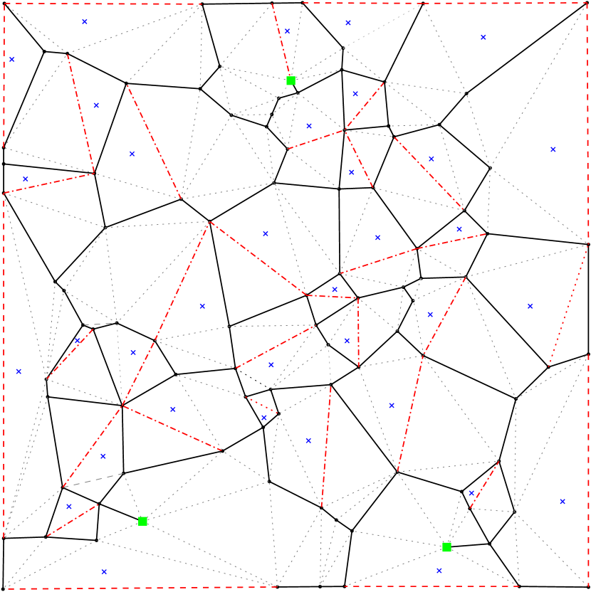
(a) Label Phase

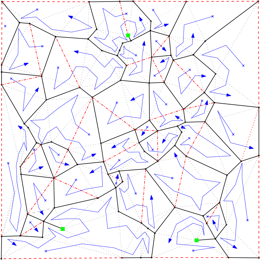
(b) Traversal phase

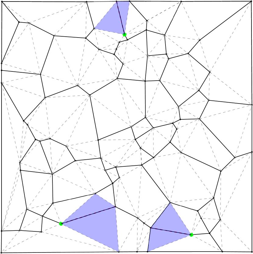
(c) Repair phase

(d) Final mesh

Figure 2: Example of generating a Polylla mesh from an initial triangulation: (a) Output of the label phase to generate terminal-edge regions. Black lines are frontier edges, dotted gray lines are internal edges, and terminal edges are red dashed lines. Terminal edges can be inside or at the boundary of the geometric domain, so dashed lines are border terminal edges, and dotted dashed lines are internal terminal edges. barrier tips are green squared vertices and seed triangles are marked with a blue cross. (b) Traversal phase example: Arrows inside terminal regions show the paths of the algorithm during the conversion from a terminal-edge region to a polygon. The path starts at a triangle labeled as a seed triangle. Each terminal-edge region has only one seed triangle. (c) Example of a non-simple polygon split using interior edges with barrier tips as endpoints. To split the polygon, the algorithm labels the middle interior edges incident to the barrier tips as frontier edges, which are then stored along with cross-labeled triangles as seed triangles. The algorithm repeats the traversal phase using a new seed triangle but avoids generating the same polygon again. (d) Final Polylla mesh. Source salinas2023generation

3.2 Polylla algorithm

The Polylla algorithm performs $3$ phases to convert terminal-edge regions $R_{i}\in\tau$ into polygons $P\in\tau^{\prime}$, those phases are show in Figure 2 and are:

1. Label Phase: each edge in the input triangulation is labeled as a terminal edge or frontier edge based on its length and adjacency to triangles. If an edge is labeled as a terminal edge, one of its adjacent triangles is chosen as a seed triangle for the next phase.

2. Traversal Phase: one seed triangle is selected from each terminal-edge region, and each polygon is generated by traversing the vertices of the frontier edges in a counter-clockwise order. Non-simple polygons with barrier edges may be generated during this phase, which are processed in the third phase.

3. Repair Phase: non-simple polygons with barrier edges are partitioned into simple polygons. Interior edges with a barrier tip as an endpoint are used to split the non-simple polygon into two new polygons. For each new polygon, a triangle is labeled as a seed and the Traversal phase is applied to generate simple polygons. The output of the algorithm is a polygonal mesh composed of simple polygons.

4 Mesh representation: CPU and GPU

Choosing the right representation is crucial to achieving good computational performance in mesh processing. In the literature, various methods exist to represent mesh geometry and topology. For example, a common approach is the triangle-based mesh representation MeshDatastructSurvey , where each triangle is represented as a set of vertices. Another option is the star-vertex representation kallmann_star-vertices_2001 , which stores important information about the mesh in the vertices. Additionally, a classic representation of a planar graph is the storage of a triangulation as an adjacency list matrix.

These three implementations are not suitable for efficient mesh generation on GPUs because they can not be easily modified to create new polygonal meshes, and because it is not possible to allocate new memory on GPUs at runtime without incurring a significant time cost. We have decided to use the half-edge data structure to represent the input and output mesh of our mesh generator because it allows us to avoid the previous issues and in addition, it is adequate for handling general polygons. The half-edge data structure, also known as Doubly Connected Edge List (DCEL) MULLER1978217 , is an edge-based data structure that represents each edge of a polygonal mesh as two half-edges of opposite orientation.

As we mentioned above, for polygonal meshes, the half-edge data structure is widely recognized for its flexibility and efficiency, with most essential queries having O(1) time complexity. The half-edge data structure also allows for a simple way to traverse inside a mesh using an edge or a face as a starting point. We have chosen this data structure for the sequential implementation and now for the GPU implementation as well. This data structure allows for a natural way to parallelize the Polylla algorithm in terms of threads per edge and triangles.

For this research, we use the half-edge implementation of our previous work shown in salinas2023generation . The implementation contains the basic half-edge queries defined in deBerg2008 , and some extended queries defined by us in salinas2023generation to facilitate the navigation inside a mesh during its generation.

4.1 Half-edge representation

(a)

(b)

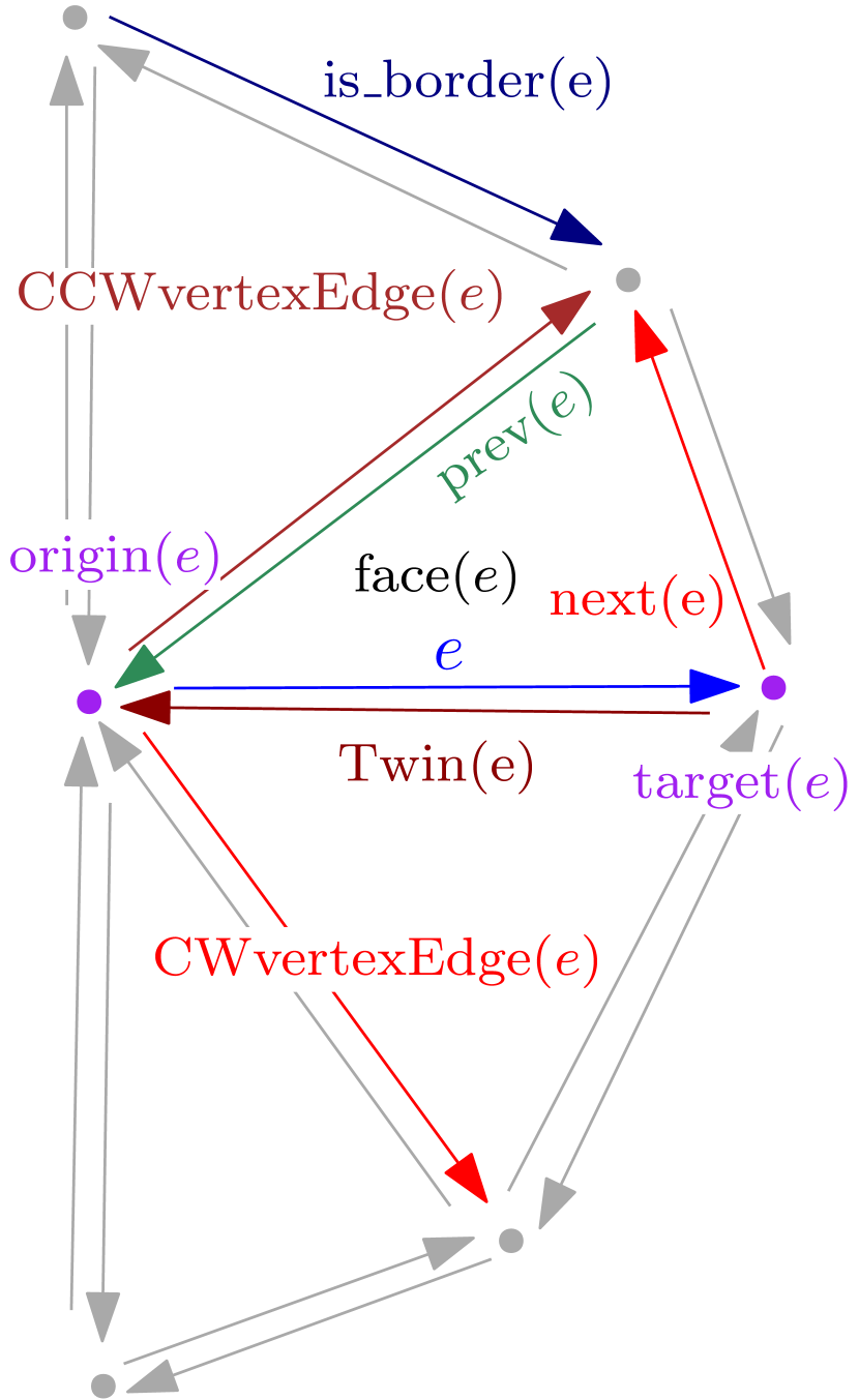
(c)

Figure 3: (a) Polygonal mesh (b) Representation of the mesh using half-edge data structure (b) Example of queries for a half-edge $e$.

Given a half-edge $e$ in a triangulation $\tau=(V,E)$ (see Figure 3), the half-edge data structure allows traversal of the face incident to $e$ through queries such as next($e$) and prev($e$), while twin($e$) enables navigation between faces. Furthermore, the structure aims the exploration of the vertices surrounding $e$ through queries like origin($e$), target($e$),

This data structure enables to define additional queries salinas2023generation . The queries CCWvertexEdge($e$) and CWvertexEdge($e$) allows traveling around the faces of $\tau$ in counterclockwise and clockwise, respectively. is_border($e$) ascertains whether a half-edge is incident to the exterior face, degree($v$) to determine the number of edges incident to a vertex $v$, incidentHalfedge($f$) to obtain a half-edge incident to a face $f\in\tau$, and edgeOfVertex($v$) to retrieve a half-edge with origin at vertex $v$.

Listing 1: Vertex record

⬇

struct vertex{

double x, y;

bool is_border;

int incident_halfedge;

};

Listing 2: Half-edge record

⬇

struct halfEdge {

int origin;

int twin;

int next, prev;

bool is_border;

};

Figure 4: Vertex and Half-edge records

4.2 Half-edge: Cuda implementation

The CUDA implementation of this data structure can be achieved using two Arrays of Structures (AoS), namely the Halfedge array and the Vertex array. These arrays provide access to the mesh information. For a detailed view of the implementation, see the Listing 1 and 2.

The half-edge data structure stores some information implicitly, which enhances its efficiency. For a triangulation, each three half-edges in the Halfedge array represent a face, enabling the incidentHalfedge($f$) query through the formula $3\cdot\#faces$. CCWvertexEdge($e$) and CWvertexEdge($e$) queries can be implemented using twin(next($e$)) and twin(prev($e$)), respectively. The query target is defined as twin(origin($e$)). The degree($v$) query is achieved by cycling around an edge incident to $v$ using the CCWvertexEdge($e$) query.

The half-edge data structure is first built on the CPU, then the HalfEdge array and Vertex array are copied to the device. On the device, the value of next and prev attributes of each half-edge are changed in such way that the input is converted from a triangular mesh to a Polylla mesh. In order to explain this strategy, Figure 5 shows two triangles being joined to create a square. In Figure 5(a) a polygonal mesh with two faces represented the half-edge data structure. On the other hand, in Figure 5(b) a change of the attribute values in the half-edges $he_{i}$ and $he_{j}$ to next($he_{i}$) = CWvertexEdge(next($he_{i}$)) and next($he_{j}$) = CWvertexEdge(next($he_{j}$)) is shown. Finally, Figure 5(c) shows the resulting polygon from joining the two triangles’ faces. The same strategy applied to join triangles can be extended to join polygons. This strategy is explained with more details in Section 5.2.

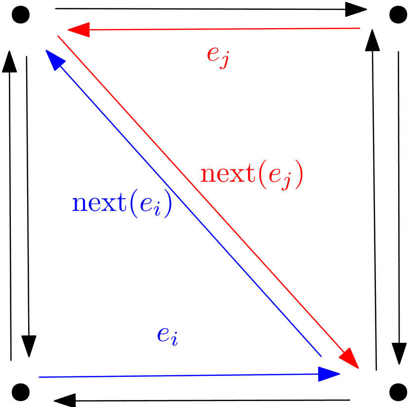
(a)

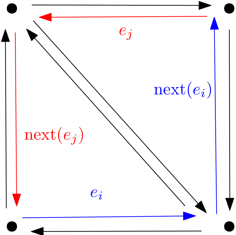
(b)

(c)

Figure 5: (a) A terminal-edge region formed by two adjacent triangles represented as the half-edge data structure. (b) The terminal-edge is dereferenced by changing the values of the next and prev of $he_{i}$ and $he_{j}$. (c) Final result of the edge elimination, a square.

This method allows us to work in the GPU without involving edge removal, which means we do not need to change the size of the allocated initial memory. The algorithm just unlinks the half edges not needed anymore. If we want to change the size of the allocated memory, we would need to copy the half-edge AoS back to the host, call the CUDA free function, ask for the new memory with CUDA malloc, and copy the new half-edge AoS to the device. However, this operation is expensive, in the experiment we will see that the copy operation between host and device has a high cost.

It is worth mentioning, that keeping the half edges of the initial triangulation, allows us to implement future mesh optimizations, such as converting non-convex polygons into convex polygons in an efficient way.

4.3 Additional data structures

Prior to the parallel implementation of the Polylla algorithm utilizing the half-edge data structure, it is necessary to establish several additional temporary data structures. Those extra data structures are different between CPU and GPU.

Secuential: In order to label each edge of the triangulation, two bit-vectors, namely longest-edge bitvector and frontier-edge bitvector, are utilized to indicate the longest edge of each triangle and frontier edges, respectively. A bit set to 1 means that the corresponding half-edge is a longest-edge or frontier-edge, respectively. The length of both bit-vectors is $2|E|$, where $|E|$ represents the number of edges of the triangulation. For the seed triangles, a seed-list stores the indices of the incident terminal edges.

In the traversal phase we do a copy of the half-edge array to change the values of the attributes next and prev, and with this, represent the half-edge of the new polylla mesh $\tau^{\prime}$. Despite this copy is optional in the secuential version, we decide to this to match with the GPU version.

During the Repair phase, two auxiliary arrays are employed to prevent the duplication of polygons, namely, an initially empty subseed-list and a usage bitvector of length E$.\par Finally,aftergeneratethePolyllamesh,theseedlistisusedtorebuildeachpolygonoftheoutputmeshusingthenextandpreviousqueriesonthathalf-edge.\par\par\par\textbf{GPU}:TheGPUimplementationusesthesamedatastructure,thearrays{\tt longest-edgebitvector}and{\tt frontier-edgebitvector}arealsothesame,inGPUthe{\tt seed-list}isa{\tt seed-bitvector}ofsize$2—E —$,andaftergeneratethePolyllameshthebitvectorisconvertedtoan{\tt outputseededges}ofintegerstofacilitatetheprocessofaccessandtraverseinthepolygonsofthePolyllamesh.\par$

5 Secuential Polylla

In this section we will talk about a new version of Polylla, used to compare the GPU accelerated version. The version presented in Salinas-Fernandez2022 used a triangle data structure to generate Polylla meshes. The version showed in salinas2023generation uses a half-edge version as input but as output have a face based data structured. And the new version presented in this paper have as input and output the half-edge data structure, this have the advantage that we can use the half-edge queries in the Polylla meshes, and we can use the same data structure for Secuential and GPU implementation to compare both versions. This new version have the same 3 phases, the label phase, the traversal phase and the repair phase. The only version in comparison salinas2023generation that change is the traversal as instead of store the polygons in a face based data structure, we copy half-edge data structure to the output mesh and modify the decencies of the queries next and prev to unlink the edges that are not part of the output mesh. The figures useful to understand each phase are the showed in Figures 2, so we will not repeat them here.

5.1 Label phase

This phase receives a triangulation $\tau=(V,E)$ as input. The objective is to label frontier-edges to identify the boundary of each terminal-edge region $R_{i}$ in $\tau$ and to select one triangle of each $R_{i}$ to be used as the seed for generating new polygons in the next phase, the Traversal phase. To do this, the phase first finds the longest edge of each triangle in $\tau$, and then labels the frontier edges and the seed edges. An example of a resulting labeled triangulation after this phase is shown in Figure 2(a). Algorithm 1 Secuential Polylla main algorithm Labeled triangulation $\tau_{L}=(V,E)$ Polylla mesh Label phase $\ignorespaces\triangleright$ Algorithm 2, 3, 4 Traversal phase $\ignorespaces\triangleright$ Algorithm 5 Repair Phase $\ignorespaces\triangleright$ Algorithm 6

Label longest-edge

For each triangle $t_{i}\in\tau$, composed by 3 half-edges, calculates which half-edge is the longest. To calculate the longest edge of each triangle $t_{i}\in\tau$ the algorithm iterates sequentially over each triangle $t\in\tau$, obtains the half-edge incident to $t_{i}$, calculates the length of the half-edges $he_{i}$, $next(e_{i})$, $prev(e_{i})$, and stores longest edge information in the longest_edge_bitvector as shown in algorithm 2. Algorithm 2 Secuential Label phase: Longest edge labeling Triangulation $\tau=(V,E)$ Labeled triangulation $\tau_{L}=(V,E)$ function CPU longest edge labeling($\tau$, longest_edge_bitvector)     for each triangle $t_{i}$ in HalfEdge do         $he_{i}\leftarrow$ incident half-edge to $t_{i}$         $d_{1},d_{2},d_{3}\leftarrow$ length size of $he_{i}$, $next(he_{i})$, $prev(he_{i})$         $he_{max}\leftarrow$ $max(d_{1},d_{2},d_{3})$         longest_edge_bitvector[$he_{max}$] = True     end for end function

Label frontier-edges

This algorithm is shown in Algorithm 3. The algorithm computes whether $he_{i}$ is a frontier-edge for each half-edge $he_{i}\in\tau$. This step takes place after the longest edge of each triangle was found and labeled in the previous phase. Thus, the algorithm for each half-edge $he_{i}\in\tau$ asks if $he_{i}$ or twin($he_{i}$) are not labeled as the longest-edge of its incident triangle in longest_edge, and if $he_{i}$ or twin($he_{i}$) are border half-edge, if one of both question is true, it is sorted in frontier-edge[$he_{i}$] as true, this mean, it labeled $he_{i}$ as a frontier-edge. Algorithm 3 Secuential Label phase: Label frontier edges Triangulation $\tau=(V,E)$ Labeled triangulation $\tau_{L}=(V,E)$ kernel LabelFrontierEdges($\tau=(V,E))$     for each halfedge $he_{i}\in\tau$ in parallel do         is_not_longest_edge? $\leftarrow$ $he_{i}$ and twin($he_{i}$) are not longest_edges         is_border_edge? $\leftarrow$ $he_{i}$ or twin($he_{i}$) is a boundary edge         if is_longest_edge? or is_border_edge? then            Label $he_{i}$ as frontier-edge         end if     end for end kernel

Label seed-edges

This algorithm is shown in Algorithm 4. In this step, we select a half-edge inside a terminal-edge region as a seed-edge, to be used to create a new polygon in the Traversal Phase. The algorithm iterates over each half-edge $he_{i}\in\tau$, for each half-edge the algorithm checks if $he_{i}$ is a terminal edge or a terminal-border edge, this is done by calculating if $he_{i}$ and twin($he_{i}$) are labels as the longest-edge in max_edge, if it is the case, one of both $he_{i}$ or twin($he_{i}$) is store in a list of integers called seed-list to use it in the Traversal phase to generate a new polygon. Algorithm 4 Secuential Label phase: Label seed edges Triangulation $\tau=(V,E)$ Labeled triangulation $\tau_{L}=(V,E)$ function LabelSeedEdges($\tau=(V,E)$)     for each halfedge $he_{i}\in\tau$ do         is_terminal_edge? $\leftarrow$ $he_{i}$ and twin($he_{i}$) are max edges and not border         is_terminal_border_edge? $\leftarrow$ $he_{i}$ or twin($he_{i}$) is max edge and border         if  is_terminal_edge? or is_terminal_border_edge?  then            Label $he_{i}$ or twin($he_{i}$) as seed-edge         end if     end for end function

5.2 Traversal Phase

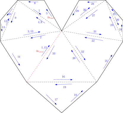
In this phase we traversal inside each terminal-edge region $R_{i}\in\tau$ to generate a polygon $P\in\tau^{\prime}$, this phase is shown in Figure 2(b). The objective of this traversal is traveling inside the frontier-edges of a terminal-edge region $R_{i}$, see Figure 6, and change the adjacencies of two continuous frontier-edges as in show in Figure 7. By changing the values of the attributies next and prev, the algorithm generate each polygon of $\tau^{\prime}$ in an implict way as was showed in Figure 5. Figure 6: Terminal-edge region $R_{i}$ to convert into a new polygon. The seed edge of $R_{i}$ is the half-edge $he_{seed}$, which is the terminal-edge of $R_{i}$. As the algorithm needs to traverse inside $R_{i}$ using the frontier-edges of $R_{i}$, the algorithms seach an frontier-edge near to $he_{seed}$ to define a $he_{init}$ and do the traversal seaching for the next frontier-edge continous to $he_{init}$. Blue arrows are the half-edges and the number is order in which each half-edge is visited by the algorithm.

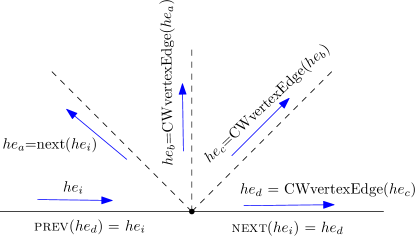
Figure 7: Example of how the algorithm uses the function CWvertexEdge to circle around a vertex and change the value of the next of a half-edge $he_{i}$. In the Figure the lines are frontier-edges, dashed lines are internal-edges and arrows are half-edges. The algorithms wants to change the next attribute of $he_{i}$, thus this circle around target($he_{i}$) until find another frontier-edge $he_{d}$ and defines next($he_{i}$) = $he_{d}$ and prev($he_{d}$) = $he_{i}$

.

As it was explained in section 4, the triangulation $\tau=(V,E)$ is represented as a half-edge data structure in a array called mesh_input array. In this phase we copy the mesh_input array to a mesh_output array to store the output mesh $\tau^{\prime}=(V,E^{\prime})$ as a half-edge data structure. The mesh_output array is the half-edge data structure that will change the values of the next and prev attributes to generate the polylla mesh $\tau^{\prime}$. The traversal phase is shown in Algorithm 5. This algorithm is a function that receives a seed edge $he_{i}$, if $he_{i}$ is a internal-edge, the algorithm circles around target($he_{i}$) until find a frontier-edge to use as begining of the traversal. Now, the algorithms defines the indices $in\,curr$, defined as the index of next($he_{init}$), and $out\,curr$, defined as the index $init$. Afterward define the initial conditions, the algorithm traverse around the terminal-edge region $R_{i}$ repeating the operation show in Figure 2(b) for each frontier-edge in $R_{i}$ until $in\,curr=init$. Afterward, the algorithm set the frontier-edge $he_{init}$ a seed thus the algorithm can use it to generate the polygon of mesh again. Notice that not all the polygons are useful for the context of meshes, some of them are non-simple polygons with barrier tips, example of those poylgons are showed in 6, the barrier tips are the green vertices. To check if a generated polygon contain barrier-edges, we start in $he_{init}$ and we traverse $P$ using the query next($he_{i}$), for each visited edge $he_{i}$ we check if $he_{i}==$ twin($he_{i}$), if this is the case, then $he_{i}$ is a barrier-edge, the polygon $P$ needs to be repaired in next phase, the repair phase. Algorithm 5 Secuential Traversal phase: Polygon construction 1:Seed edge $he$, Input Half-edge array mesh_input, Output Half-edge array mesh_output 2:Output Half-edge array mesh_output with the half-edge attributes modified. 3:while $he$ is not a frontier-edge do 4:    $he$ $\leftarrow$ CWvertexEdge($he$) 5:end while 6:${init}$ $\leftarrow$ index of $he$ 7:${in\,curr}$ $\leftarrow$ next(mesh_input[$init$]) 8:${out\,curr}$ $\leftarrow$ ${init}$ 9:repeat 10:    while mesh_input[$init$] is not a frontier-edge do 11:        ${in\,curr}$ $\leftarrow$ CWvertexEdge(mesh_input[$init$]) 12:    end while 13:    mesh_output[$out\,curr$].next $\leftarrow$ $in\,curr$ 14:    mesh_output[$in\,curr$].prev $\leftarrow$ $out\,curr$ 15:    $in\,curr$ $\leftarrow$ next(mesh_input[$in\,curr$]) 16:until ${init}=in\,curr$ 17:Set half-edge mesh_output[$init$] as seed edge

5.3 Repair phase

This phase is shown in the algorithm 6. This algorithm is a polygon $P$ with barrier tips, and it splits the polygon until it removes all barrier tips. The output is a set of seed half-edges that represent the new polygons generated in this phase. Despite on the changes made in the label phase and traversal phase, this phase is the same as the showed in Salinas-Fernandez2022 ; salinas2023generation without any modification.

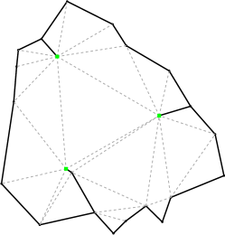
(a)

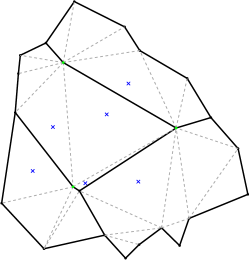
(b)

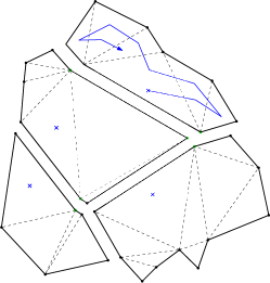
(c)

Figure 8: Example of a non-simple polygon split using interior edges with barrier tips as endpoints. (a) Non-simple polygon. (b) Middle interior edges incident to barrier tips are labeled as frontier-edges (solid lines), and cross-labelled triangles are stored as seed triangles. (c) The algorithm repeats the travel phase using a new seed triangle but avoiding generating the same polygon again. Source: Salinas-Fernandez2022 ; salinas2023generation . For each barrier tip $b_{i}\in P$, it calculates the middle edge that contains $b_{i}$. It then labels the edges of the middle edge as frontier-edges, uses them as seed edges, stores in a list them in a list called subseed-list, and labels them as True in usage bitvector, to mark them as visited during this phase. After finding all barrier tips, the algorithm generates polygons from the half-edge $he_{i}\in$ subseed-list using the Algorithm 5 of the traversal phase, only half-edge that are in subseed-list and usage bitvector are used as seed-edges. If a half-edge of the subseed-list is visited during the traversal, then it is removed from subseed-list and labeled as False in usage bitvector. Algorithm 6 Secuential Repair phase Seed edge of a non-simple polygon $P$ Set of simple polygons $S$ Initialize subseed list as $L_{p}$ and usage bitarray as $A$ $S\leftarrow\emptyset$ for each barrier tip $b$ in $P$ do     $e\leftarrow$ edgeOfVertex($b$)     while $e$ is not a frontier-edge do         $e\leftarrow$ CWvertexEdge($e$)     end while     for 0 to $(\textsc{degree}(b)-1)/2$ do         $e\leftarrow$ CWvertexEdge($e$)     end for     Label $e$ as frontier-edge     Save half-edges $he_{1}$ and $he_{2}$ of $e$ in $L_{p}$     $A[he_{1}]\leftarrow\texttt{True}$, $A[he_{2}]\leftarrow\texttt{True}$ end for for each half-edge $h$ in $L_{p}$ do     if $A[h]$ is True then         $A[h]\leftarrow\texttt{False}$         Generate new polygon $P^{\prime}$ starting from $h$ using Algorithm 5.         Set as False all indices of half-edges in $A$ used to generate $P^{\prime}$     end if     $S\leftarrow S\cup P^{\prime}$ end for return $S$

6 GPU Polylla

In this section, we introduce the GPU accelerated algorithms. The GPU variant does not have the same phases as the sequential version. In this version the label phase is almost the same as the Secuential version, but the traversal phase and the repair phase are different. For clariffication, a kernel a function that gets executed on GPU. A summary of the GPU algorithm is shown in Algorithm 7. The GPU variant have a total of 6 kernels. In each subsection we will explain one of them. This algorithm takes as input a triangulation $\tau(V,E)$ and generates as output a polygonal mesh, where the output is a half-edge representation of the polygonal mesh $\tau^{\prime}(V,E)$. In the following subsections we are going to explain each kernel called during the algorithm execution. Each kernel is called in the order showed here and with only a sync barrier between each kernel, this barrier is to force to the algorithm to wait until all threads ends to launch the next kernel. Algorithm 7 GPolylla main algorithm triangulation $\tau=(V,E)$ Polylla mesh $\tau^{\prime}=(V,E)$ Label the longest-edge of each triangle $\ignorespaces\triangleright$ Algorithm 8 Label frontier edges $\ignorespaces\triangleright$ Algorithm 9 Label seed edges $\ignorespaces\triangleright$ Algorithm 10 Label extra seed and frontier edges $\ignorespaces\triangleright$ Algorithm 11 Change attributes $\ignorespaces\triangleright$ Algorithm 12 Search frontier edges for each seed edge $\ignorespaces\triangleright$ Algorithm 13 Overwritte seeds $\ignorespaces\triangleright$ Algorithm 14 Scan and compact seed edges array

6.1 GPU longest edge labeling

GPolylla starts by calculating the longest-edge of each triangle, this is made to define the border of each terminal-edge region $R_{i}$ and the seeds that will be use to access to polygon of $\tau^{\prime}$. The kernel to calculating of the longest-edge is shown in Algorithm 8, it is the direct equivalent to the secuential Algorithm showed in Section 5.1. For each triangle in $\tau$, the algorithm assign one half-edge $he_{i}$, that is part of the interior of the triangle, to each thread of the GPU. Then, the kernel calculates length of the half-edge $he_{i}$, $next(he_{i})$ and $prev(he_{i})$ and mark which is the longest in the longest_edge_bitvector. Algorithm 8 GPU Label phase longest edge labeling Triangulation $\tau=(V,E)$ Labeled triangulation $\tau_{L}=(V,E)$ kernel GPU Label longest edge labeling($\tau$, longest_edge_bitvector)     for each halfedge $he_{i}$ in $\tau$ in parallel  do         $d_{1},d_{2},d_{3}\leftarrow$ length size of $he_{i}$, $next(he_{i})$, $prev(he_{i})$         $he_{max}\leftarrow$ $max(d_{1},d_{2},d_{3})$         longest_edge_bitvector[$he_{max}$] = True     end for end kernel

6.2 GPU frontier-edges labeling

In this kernel we calculate the border of a terminal-edge region $R_{i}$ using the longest_edge_bitvector created in the previous kernel. This is done by computing if $he_{i}\in\tau$ is a frontier-edge and it is the direct equivalent to the secuential Algorithm showed in Section 5.1. The kernel is showed in 9. The algorithm assign a thread to each half-edge $he_{i}\in\tau$. The kernel uses the longest_edge_bitvector to check if $he_{i}$ is not the longest-edge edge of its incident triangle and to triangle that contains twin($he_{i}$). If it is the case, them $he_{i}$ is a frontier-edge and is mark as true in frontier-edge bitvector[$he_{i}$]. If $he_{i}$ is a border-edge then it is marked as true. Algorithm 9 Secuential Label phase: Label frontier edges Triangulation $\tau=(V,E)$ Labeled triangulation $\tau_{L}=(V,E)$ kernel LabelFrontierEdges($\tau=(V,E))$     for each halfedge $he_{i}\in\tau$ in parallel do         is_not_longest_edge? $\leftarrow$ $he_{i}$ and twin($he_{i}$) are not longest_edges         is_border_edge? $\leftarrow$ $he_{i}$ or twin($he_{i}$) is a boundary edge         if is_longest_edge? or is_border_edge? then            Label $he_{i}$ as frontier-edge         end if     end for end kernel

6.3 GPU seed-edges labeling

In this phase, the algorithm labels those half-edges that are terminal-edges using the longest_edge_bitvector in the seed_edge_bitvector. The algorithm selects these half-edges as seeds half-edges because there is only one terminal-edge within a terminal-edge region $R_{i}$, and this edge can be used to generate the polygon after changing the adjacencies of the frontier-edges. The kernel is shown in Algorithm 10. For each half-edge $he_{i}$ in $\tau$, the kernel checks if both $he_{i}$ and twin($he_{i}$) are marked as the longest edge in longest_edge and if neither is a border-edge. This indicates that both are terminal-edges. Conversely, if $he_{i}$ or twin($he_{i}$) is marked as the longest edge in longest_edge and one of them is a border-edge, this indicates they are border terminal-edges. If one condition is true, then the half-edge between $he_{i}$ and twin($he_{i}$) is labeled as a seed edge in the resulting bit-vector seed-bitvector. It’s worth noting that the bit-vector seed-bitvector is a sparse array that contains zeros and ones, which makes it sub-optimal for the traversal phase. Since we cannot determine the exact number of seed edges in advance, we need to assign one seed edge to each thread during this phase. Algorithm 10 Label seed edge Triangulation $\tau=(V,E)$ Labeled triangulation $\tau_{L}=(V,E)$ kernel LabelSeedEdges($\tau=(V,E))$     for each halfedge $he_{i}\in\tau$ in parallel do         is_terminal_edge? $\leftarrow$ $he_{i}$ and twin($he_{i}$) are max edges and not border         is_terminal_border_edge? $\leftarrow$ $he_{i}$ or twin($he_{i}$) is max edge and border         if  is_terminal_edge? or is_terminal_border_edge?  then            Label $he_{i}$ or twin($he_{i}$) as seed-edge         end if     end for end kernel

6.4 Label extra seed and frontier edges

In order to do the repair phase in parallel, we have to do this extra step, in this phase the algorithm convert internal-edges adjacent to a barrier tip to frontier-edges, thus the algorithm avoid generates non-simple polygons in the first place. The kernel called in this step is shown in Algorithm 11, notice that this kernel is the equivalent of the first part of the repair phase showed in Algorithm 6. For each vertex in $v_{i}\in\tau=(V,E)$, the kernel count the number of frontier-edges adjacent to $v_{i}$, if there is only one frontier-edge adjacent to $v_{i}$, then $v_{i}$ is a barrier tip, thus the kernel count the number of edges adjacent to $v_{i}$, and select one of them, the middle one counting from a frontier-edge, and convert the internal-edge to a frontier-edge, labeling their two half-edges as frontier-edges and as seed-edges, thus the algorithm can use them to generate to new polygons. The part of store two new seed half-edges must be done, as is show in Figure 8, a non-simple polygon only have one seed to generate that polygon, but it could generate several new polygons after repair it. All those new polygons needs a seed to be generated too, thus the algorithm needs to store multiple new seeds, the problem with this addition, is one polygon could have more of one seed. But it will be fixed in the kernel of the subsection 6.6. Algorithm 11 Label Extra Frontier Edge Labeled $\tau_{L}=(V,E)$ Updated $frontier\_edges$ and $seed\_edges$ kernel label_extra_frontier_edge_d($\tau=(V,E)$)     for each vertices $v_{i}\in\tau$ in parallel do         $he$ $\leftarrow$ edgeOfVertex($v_{i}$)         numFrontierEdges $\leftarrow$ 0         repeat $\ignorespaces\triangleright$ Count frontier-edges adjacent to $v_{i}$            if $he$ is a frontier-edge then                numFrontierEdges $\leftarrow$ numFrontierEdges + 1            end if            $he\leftarrow$ CWvertexEdge($he$)         until $he$ is not edgeOfVertex($v_{i}$)         if numFrontierEdges is equal to 1 then $\ignorespaces\triangleright$ If $v_{i}$ is barrier tip            $he\leftarrow$ edgeOfVertex($v_{i}$)            while $he$ is not a frontier-edge do $\ignorespaces\triangleright$ Find middle edge                $he\leftarrow$ CWvertexEdge($he$)            end while            for 0 to $(\textsc{degree}(v_{i})-1)/2$ do $\ignorespaces\triangleright$ set $he$ as middle edge                $he\leftarrow$ CWvertexEdge($he$)            end for            Label $he$ and twin($he$) as frontier-edge            Label $he$ and twin($he$) as seed-edges         end if     end for end kernel

6.5 Change attributes

After labeling the frontier-edges and seed-edges, the algorithm can start the process of changing the adjacencies of the attributes of each half-edges showed in Algorithm 5. The kernel that do this is showed in Algorithm 12. For each half-edge $he_{i}\in\tau$ in parallel, the kernel search the next and previous frontier-edge, using the same idea showed in Figure 2(b), but in the case of the search of the previous frontier-edge, the algorithm uses the CCWvertexEdge query instead of the CWvertexEdge($he$). Algorithm 12 GPU Change atributes kernel Labeled triangulation $\tau_{L}=(V,E)$ Polylla mesh kernel Traversal phase($\tau_{L}=(V,E)$)     for each halfedge $he_{i}$ in $\tau_{L}$ in parallel  do         next $\leftarrow$ $he_{i}$         while next is not a frontier-edge do $\ignorespaces\triangleright$ Search next frontier-edge in CW            next $\leftarrow$ CWvertexEdge($he$)         end while         set_next(next($he_{i}$)) $\leftarrow$ next         prev $\leftarrow$ $he_{i}$         while prev is not a frontier-edge do $\ignorespaces\triangleright$ Search prev frontier-edge in CCW            prev $\leftarrow$ CCWvertexEdge($he$)         end while         set_prev(prev($he_{i}$)) $\leftarrow$ prev     end for end kernel

6.5.1 Search frontier edges for each seed edge

At this point, the algorithm already have a Polylla mesh in the half-edge data structure, but there are two problems, some seeds are internal-edges of the triangulation and not half-edges of the Polylla mesh, and there are some polygons with more of one seeds to generate it. In this kernel we are going to solve the first problem. The reason of why there are seed that are internal edges is because when the algorithm does the process of label the seed-edges we choose one of the two half-edges of the terminal-edges as a seed half-edge. In the kernel showed in Algorithm 13 for each seed half-edge the algorithm search a new frontier-edge using the operation CWvertexEdge and after find one, the algorithm remove the label of the seed half-edge and label the found frontier-edge as a new seed edge. After this kernel the algorithm only need to remove extra seed half-edges to complete the Polylla mesh. Algorithm 13 GPU Search frontier edges for each seed edge Labeled triangulation $\tau_{L}=(V,E)$ Polylla mesh kernel Traversal phase($\tau_{L}=(V,E)$)     for each halfedge $he_{i}$ in $\tau_{L}$ in parallel  do         if $he_{i}$ is a seed edge then            next $\leftarrow$ $he_{i}$            while next is not a frontier-edge do $\ignorespaces\triangleright$ Search next frontier-edge in CW                next $\leftarrow$ CWvertexEdge($he_{i}$)            end while            if next is not $he_{i}$ then                seed_edge_bitvector[$he_{i}$] = False $\ignorespaces\triangleright$ Set the frontier-edge a a seed edge            end if            seed_edge_bitvector[$he_{i}$] = True $\ignorespaces\triangleright$ Remove the original seed edge         end if     end for end kernel

6.6 Overwritte seeds

Note that in the kernel presented in subsection 6.4, the algorithm labels two adjacent half-edges to an interior-edge as frontier-edges to split a non-simple polygon. To ensure that the new polygons have a seed, the algorithm also labels both half-edges as seed edges. However, this poses a problem because the algorithm might generate the same polygon twice. To prevent this, the algorithm overwrites the seed half-edges using the kernel presented in Algorithm 14. For each seed half-edge, the kernel traverses inside the polygon that generated the seed. During this traversal, it searches for the frontier half-edge with the smallest index and labels this half-edge as a seed half-edge. To avoid race conditions, the algorithm first checks if the minimum index $min$ is not equal to the index of the original seed $i$. If this is true, the algorithm sets seed_edge_bitvector[$i$] to False. Subsequently, it sets seed_edge_bitvector[$min$] of the frontier-edge with the minimum index to True. It is important to note that this kernel is also implemented in the sequential algorithm, specifically in the repair phase as outlined in 5.3. The algorithm 6 is divided into two kernels: the first part is executed in Kernel 6.4, and the second part is executed in the kernel described in this subsection. Algorithm 14 GPU Overwritte seeds Labeled triangulation $\tau_{L}=(V,E)$ Polylla mesh kernel Traversal phase($\tau_{L}=(V,E)$)     for each halfedge $he_{i}$ in $\tau_{L}$ in parallel  do         ${init}$ $\leftarrow$ $he_{i}$         ${min}$ $\leftarrow$ ${init}$         ${curr}$ $\leftarrow$ next(init)         while init is not curr do            min $\leftarrow$ minimum(min, curr)            curr $\leftarrow$ next(curr)         end while         if min is not $he_{i}$ then            seed_edge_bitvector[$he_{i}$] = False         end if         seed_edge_bitvector[${min}$] = True     end for end kernel

6.7 Scan and compact seed edges array

Until this kernel we already have a polylla mesh generated, but the output seed edges are in a bitvector and to be converted to integer array. This is done with the classical scan and compact technique, but accelerate with tensor cores In this kernel the algorithm used a technique based on prefix sum to compact the seed-edges array, which was also used in carrasco2023evaluation . This technique consists of computing the prefix sum of all elements of the seed-list bit-vector, this sum says the location in the compacted output array. This step is not equivalent to any step in the secuential algorithm as in the secuential algorithm the seed edges are stored in a list, but in the GPU algorithm the seed edges are stored in a bit-vector, thus the algorithm needs to convert the bit-vector to a list.

7 Experiments

This section describes the experimentation conducted in this study, including the dataset utilized, tests carried out (experiments and benchmark environment), and the results obtained.

7.1 Dataset

The Figure 9 shows two different point distributions that we used to test out our algorithm. The first one, in Figure 9(a), is a totally uniform grid, this kind of grid is generated using the Algorithm 15. The second one is shown in Figure 9(b), it is a Delaunay mesh generate using random uniform points, this kind of mesh is generated by randomly placing points on a square, without overlapping points, and using a tolerance parameter $\delta$ to move the points that are near to the border of the square to the border, afterward using the software Triangle triangle2d to generate a Delaunay mesh. For the rest of the experiments we will call to the first kind of mesh a Grid meshes and to the second a Random meshes.

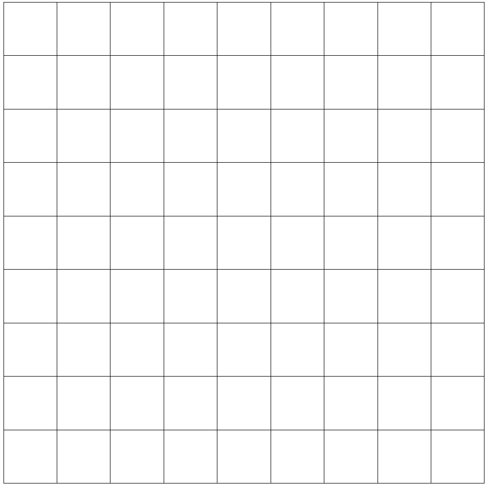
(a) Uniform Distribution

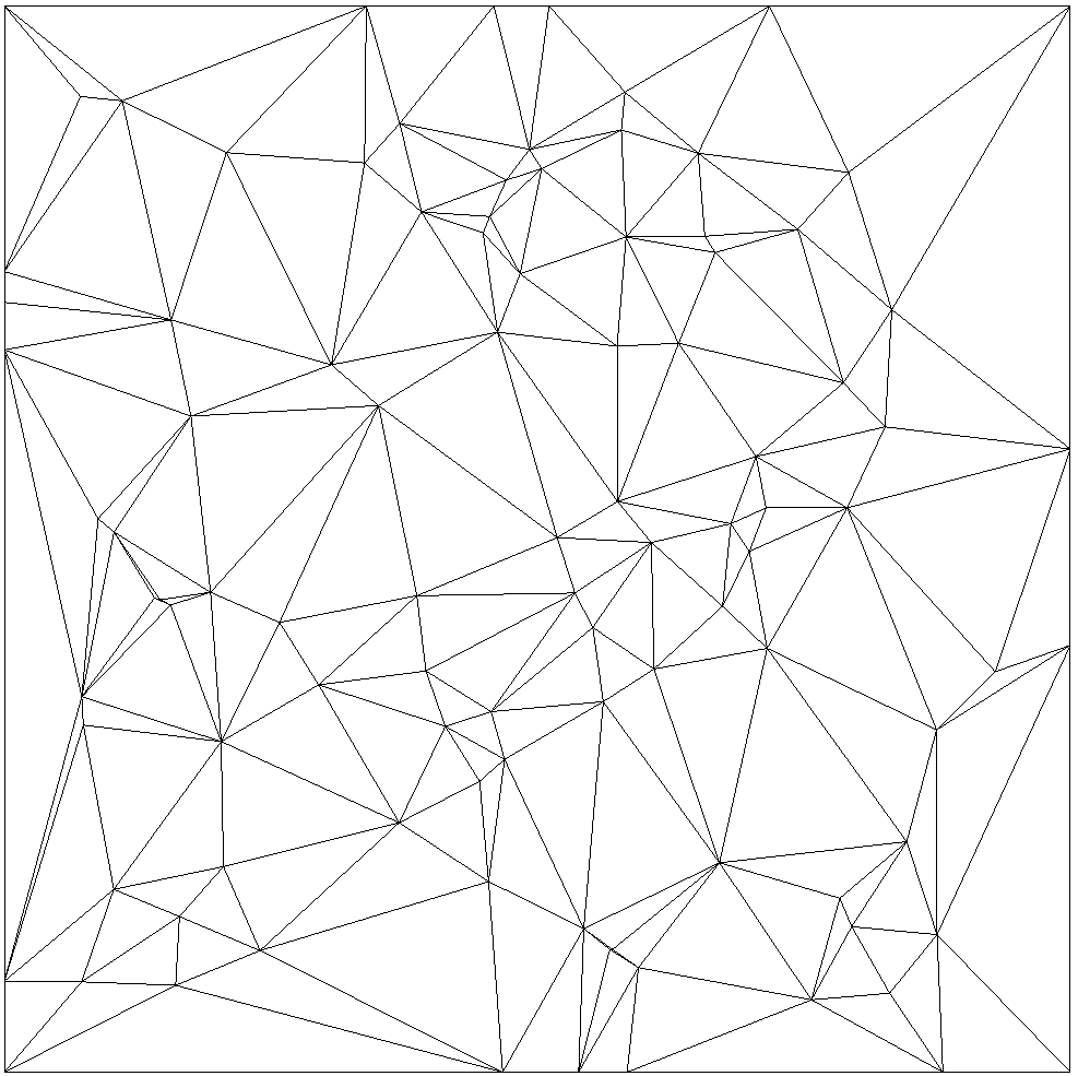
(b) Delaunay distribution

Figure 9: The illustration shows both input tests of our experiment, the left one is a uniform grid with the 100 closest equidistant square roots perfect, and on the right is an example of 100 points on a Delaunay distribution. Algorithm 15 Generate points and triangles for a 2D mesh $n>1$ List of vertices and triangle indices for a 2D mesh with $n$ points procedure GenerateMesh($n$)     Create an empty list of vertices $Vertices$     Create an empty list of triangle indices $faces$     $sqrt\_n\leftarrow\lfloor\sqrt{n}\rfloor$     for each $i$ from $0$ to $\text{sqrt\_n}-1$ do         for each $j$ from $0$ to $\text{sqrt\_n}-1$ do            Create a new vertex $ve$ with coordinates $(i,j)$            Add $ve$ to the list $Vertices$         end for     end for     for each $i$ from $0$ to $n-\text{sqrt\_n}-1$ do         if $i\bmod\text{sqrt\_n}\neq\text{sqrt\_n}-1$ then            Add $i$ to the list $faces$            Add $i+1$ to the list $faces$            Add $i+\text{sqrt\_n}+1$ to the list $faces$            Add $i$ to the list $faces$            Add $i+\text{sqrt\_n}+1$ to the list $faces$            Add $i+\text{sqrt\_n}$ to the list $faces$         end if     end for     return $Vertices$, $faces$ end procedure

7.2 Experimental setup

Our implementation employed C++ with -O3 optimization for the CPU component and CUDA with NVCC 12 for the GPU component. We conducted all of our experiments on the Patagón supercomputer patagon , which is equipped with a single Nvidia DGX A100 GPU node, two AMD EPYC 9534 CPUs with 64 cores and 256MB L3 cache, 756 GB of RAM DDR5, and 3 Nvidia L40 GPUs, each with 48GB of VRAM GDDR with ECC. However, for the purposes of our experiments, we utilized only a single L40 GPU. The present work explores and compares the effectiveness of different point distributions through the implementation of two experiments. The first experiment involved utilizing a Delaunay distribution with 32 equidistant intervals ranging from one million to 46 million points. The second experiment employed a uniformly distributed grid with the 32 nearest roots to the equidistant intervals between one million and 100 million. These experiments were limited by the current memory constraints of graphics cards, as the author attempted to reach the maximum number of points that their current hardware could support. However, it is important to note that there are no such limitations at the programming level, and it is possible to scale the number of points as new hardware with higher capacity becomes available.

7.3 Results

CPU GPU #V LM LF LS Trav Rep Total CtD LLK LFK LSK LEK CaK SFK BtH OSK Scan TwC Total 1M 917.0 256.0 333.8 361.1 43.8 1911.8 7.0 0.4 0.2 0.2 1.2 0.4 0.2 8.8 0.3 0.3 19.0 3.2 12M 11246.7 3037.6 3943.3 4274.7 538.4 23040.8 80.7 5.4 2.8 2.7 25.8 4.6 2.2 100.0 3.1 1.8 229.1 48.4 23M 21727.2 5817.2 7555.6 8263.2 1046.8 44410.1 153.7 10.3 5.3 5.2 50.3 8.8 4.1 195.7 5.8 3.3 442.5 93.2 33M 32300.9 8590.3 11173.1 12165.1 1549.6 65779.0 227.3 15.2 7.9 7.6 74.9 13.0 6.0 281.0 8.6 4.7 646.1 137.9 44M 42827.9 11451.2 14751.8 16122.6 2046.5 87200.0 299.9 20.0 10.4 10.0 99.2 17.2 8.0 419.4 11.4 6.2 901.7 182.4 1M 675.5 178.8 274.0 303.8 0.0 1432.0 7.1 0.4 0.2 0.2 0.4 0.3 0.2 9.0 0.2 0.3 18.3 2.2 27M 18215.8 4855.4 7341.4 8241.9 0.0 38654.5 179.7 8.8 6.4 6.5 8.3 10.1 4.3 237.9 4.8 4.2 470.9 53.3 49M 33451.3 8912.5 13485.0 15180.5 0.0 71029.3 332.1 15.9 11.8 11.9 15.1 18.6 7.8 436.8 8.9 7.5 866.5 97.6 74M 51456.9 13746.1 20822.9 23551.0 0.0 109577.0 522.0 24.1 18.1 18.2 22.9 28.4 11.8 876.9 13.5 11.4 1547.2 148.3 100M 68806.4 18513.8 27816.8 31814.4 0.0 146951.4 741.0 32.1 24.4 24.6 30.3 38.1 15.8 1027.5 18.1 15.2 1967.0 198.4 Table 1: Time measurements for the CPU and GPU versions of Polylla. The times are in miliseconds. The upper table is the Random meshes and the lower table is the Grid meshes. The table presents the number of vertices (#V) for each mesh, along with the timings for different stages of the algorithm. For the CPU version: ”Label the longest-edge” (LM), ”Label frontier edges” (LF), ”Label seed edges” (LS), ”Traversal phase” (Trav), and ”Repair phase” (Rep), cumulating in the total time for CPU Polylla (Total). The GPU version encompasses: ”Copy to Device” (CtD), ”Label the longest-edge kernel” (LLK), ”Label frontier edges kernel” (LFK), ”Label seed edges kernel” (LSK), ”Label extra seed and frontier edges kernel” (LEK), ”Change attributes” (CaK), ”Search frontier edges for each seed edge” (SFK), ”Overwrite seeds” (OSK), ”Scan and compact seed edges array” (Scan), ”Copy back to Host” (BtH), culminating in the total time for GPU Polylla excluding copy times (Total).

(a) CPU random meshes

(b) CPU grid meshes

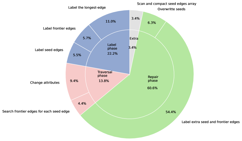
(c) GPU random meshes

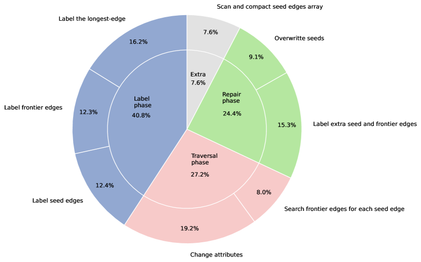
(d) GPU grid meshes

Figure 10: Comparison of CPU and GPU Performance of each phase of the algorithm. In the case of random meshes we present the result for 44 millon points case, for the grid meshes we present we 100 millons case.

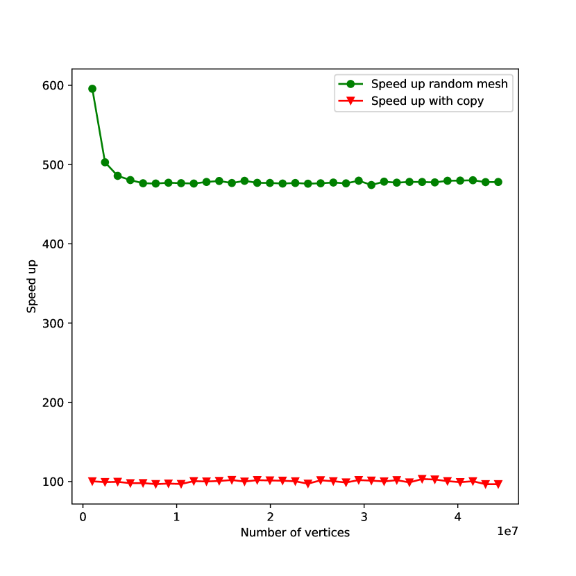
(a) Random meshes

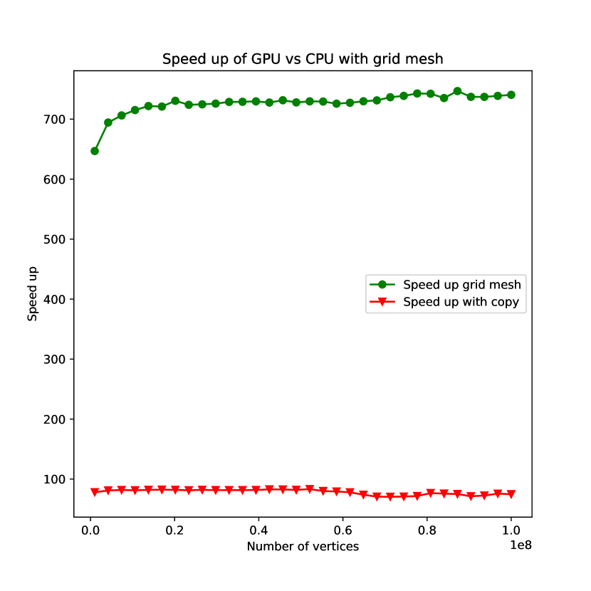
(b) Grid meshes

Figure 11: The illustration shows both input tests of our experiment, the left one is a uniform grid with 32 closest equidistant perfect square roots, and on the right is an example of 32 points on a Delaunay distribution.

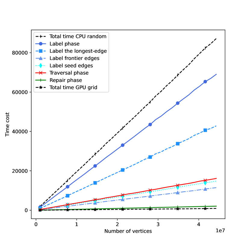
(a) Random meshes

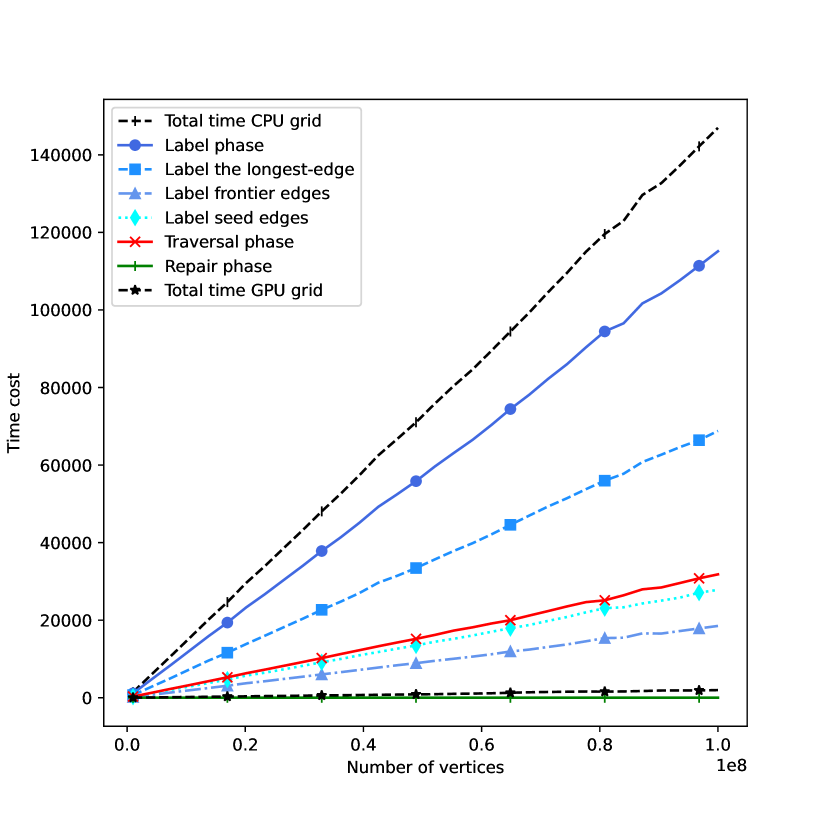
(b) Grid meshes

Figure 12: The illustration shows both input tests of our experiment in CPU and GPU including the repair phase, the left one is a uniform grid with 32 closest equidistant perfect square roots, and on the right is an example of 32 points on a Delaunay distribution. Table 1 shows the duration of each phase in our CPU and new GPU implementation, along with the time taken for copying to the device for 5 of the 32 experiments of the Random meshes and Grid meshes. The rest of the table can be seen in Appendix A. We can see that the maximum speed up the Random meshes is of $\times 595.6$, and if we considerate the copy is of $\times 103.2$ In the case of the Grid meshes the maximum speed up is of $\times 746.8$ and $\times 83.2$ with copy. Those speed up are show in the Figure 11. Notice that copy the data structure from host to device and copy from device to host is a $79\%$ in average of the total time of the algorithm. To compare the time cost of each phase in the secuential algorithm and the cost of each kernel in the GPU, we do a pie chart with last rows of the Table 1. In those pie chart we define the kernels of the equivalent phase in the secuential, the only kernel without equivalent is the scan as it is only necessary in the GPU due to the uses of a bitvector to store the output seeds. The charts we can see that kernel related to the repair phase are the most time cost of the algorithm, and even when there are no barrier tips to repair, as it is case of the Grid meshes, there is a cost in the kernel “Label extra seed and frontier edges” as in this kernel, for each vertex in the triangulation, the algorithm have to check if the vertex is a barrier tip or is not. The “Overwrite seed kernel” will also have a cost as in this phase we the algorithm set the edge with the minimum index as an output seed edge, when there are barrier tip this aviod to have repited polygon, but when there are not barrier tip, this kernel is no necessary. In the case of the Label phase, the label longest-edge is the most time cost step in both CPU and GPU, but the GPU acceration help to avoid made this process the most costly process in all the algorithm for the Random meshes. Finally, to compare to present the magnitude of the low time cost of the GPU Polylla in comparision with the secuential Polylla, the Figure 12 show as the GPU Polylla algorithm is even lower in time than the secuential repair phase. In Figure 12(b), the GPU algorithm lost againts the repair phase only becouse there is no repair phase in those meshes, thus the time cost is $0$.

8 Conclusions and ongoing work

In this work, we showed a novel way to generate polygonal meshes in GPU, the way that we modify the attributes of each half-edge structure to simulate edge removition and join faces polygonal faces, can be used in the future to accelerate the process that requires mesh simplification in GPU, as can be low polygon mesh generation. Notice that this work is a fully GPU algorithm, the only need of CPU time is to generate the data structure and send it to the GPU. In conclusion, our algorithm running on a GPU has proven to be highly scalable, allowing for larger meshes to be processed simply by increasing the available graphics memory. We can get a maximum speed up of $\times 746.8$, and if we consider a more realistic case, as a meshes with points in general position (the random meshes) and considering the copy time from device to host and host to device, we can get a speed up of $\times 83.2$. As the generations of GPUs progress, the graphic’s memory continues to increase, enabling even larger meshes to be processed. Additionally, the performance of the algorithm can be improved by enhancing the speed of transfer between the GPU and CPU, which accounts for 79% of the algorithm. Future work for the GPolylla algorithm is using the compact data structure presented in our previous work salinas2023generation to get even bigest meshes, but with one reduction of the speed up.

9 Acknowledgment

This research was supported by the Patagón supercomputer patagon-uach of Universidad Austral de Chile (FONDEQUIP EQM180042). This work was partially funded by ANID doctoral scholarship 21202379 (first author), ANID doctoral scholarship 21210965 (second author), and ANID FONDECYT grant 1211484 (third author).

Appendix A Tables

Here we have the tables used to generate the plots in section 7. Table LABEL:Fig:table_random_Total is the table with the CPU and GPU times of the random meshes, and Table LABEL:Fig:table_grid_Total of the Grid meshes. CPU GPU #V LM LF LS Trav Rep Total CtD LLK LFK LSK LEK CaK SFK BtH OSK Scan TwC Total 1000000 917.0 256.0 333.8 361.1 43.8 1911.8 7.0 0.4 0.2 0.2 1.2 0.4 0.2 8.8 0.3 0.3 19.0 3.2 2353515 2202.2 608.6 786.3 851.6 105.6 4554.3 16.2 1.1 0.6 0.6 4.5 0.9 0.5 20.6 0.6 0.4 45.8 9.1 3707030 3481.0 950.6 1240.0 1337.6 167.7 7177.0 25.4 1.7 0.9 0.9 7.5 1.4 0.7 31.8 1.0 0.7 72.0 14.8 5060545 4783.0 1304.8 1696.7 1834.0 232.0 9850.6 34.6 2.3 1.2 1.2 10.6 2.0 1.0 45.5 1.3 0.9 100.5 20.5 6414060 6046.3 1648.7 2136.4 2314.1 292.8 12438.3 43.9 2.9 1.5 1.5 13.7 2.5 1.2 56.8 1.7 1.1 126.8 26.1 7767575 7341.3 1994.7 2588.9 2823.8 353.5 15102.2 52.9 3.5 1.8 1.8 16.8 3.0 1.5 71.3 2.0 1.2 155.9 31.7 9121090 8691.1 2355.0 3052.4 3318.1 419.2 17835.8 62.0 4.2 2.2 2.1 19.9 3.6 1.7 83.6 2.4 1.4 183.0 37.4 10474605 9979.0 2687.9 3511.3 3802.3 475.2 20455.7 71.3 4.8 2.5 2.4 22.9 4.1 1.9 96.7 2.7 1.6 210.9 42.9 11828120 11246.7 3037.6 3943.3 4274.7 538.4 23040.8 80.7 5.4 2.8 2.7 25.8 4.6 2.2 100.0 3.1 1.8 229.1 48.4 13181635 12592.3 3381.6 4417.0 4766.7 606.7 25764.4 89.7 6.0 3.1 3.0 28.8 5.1 2.4 113.7 3.4 2.0 257.3 53.9 14535150 13883.2 3733.7 4872.0 5333.8 671.6 28494.4 98.5 6.6 3.4 3.4 31.9 5.7 2.7 124.7 3.8 2.1 282.7 59.5 15888665 15202.4 4064.6 5318.9 5699.3 724.6 31009.8 107.8 7.2 3.8 3.6 34.9 6.2 2.9 131.3 4.1 2.3 304.1 65.1 17242180 16545.0 4482.0 5779.2 6302.0 798.5 33906.7 117.0 7.8 4.1 4.0 38.0 6.7 3.1 151.2 4.5 2.5 338.9 70.7 18595695 17832.9 4778.3 6216.1 6722.0 856.6 36405.9 126.0 8.4 4.4 4.3 41.1 7.3 3.4 155.2 4.8 2.7 357.5 76.3 19949210 19130.3 5143.9 6667.7 7222.8 916.7 39081.3 135.4 9.1 4.7 4.6 44.2 7.8 3.6 168.0 5.1 2.9 385.3 82.0 21302725 20425.9 5494.6 7109.7 7707.9 978.0 41716.1 144.5 9.7 5.0 4.9 47.3 8.3 3.9 180.3 5.5 3.1 412.5 87.6 22656240 21727.2 5817.2 7555.6 8263.2 1046.8 44410.1 153.7 10.3 5.3 5.2 50.3 8.8 4.1 195.7 5.8 3.3 442.5 93.2 24009755 23022.5 6166.4 7999.8 8670.9 1101.9 46961.4 163.0 10.9 5.7 5.5 53.3 9.4 4.4 220.6 6.2 3.5 482.4 98.7 25363270 24414.3 6500.9 8449.3 9124.3 1178.0 49666.8 171.6 11.5 6.0 5.8 56.4 9.9 4.6 212.8 6.5 3.6 488.7 104.3 26716785 25813.9 6828.1 8889.6 9664.0 1237.3 52432.9 181.1 12.1 6.3 6.1 59.4 10.4 4.8 230.9 6.9 3.8 521.9 109.9 28070300 26987.9 7188.0 9346.4 10162.0 1293.3 54977.6 190.1 12.7 6.6 6.4 62.5 10.9 5.1 250.5 7.2 4.0 556.0 115.4 29423815 28639.1 7563.8 9806.0 10631.2 1377.3 58017.4 199.4 13.3 6.9 6.7 65.5 11.5 5.3 249.1 7.6 4.2 569.4 121.0 30777330 29646.2 7923.9 10244.3 11172.6 1427.1 60414.0 208.6 13.9 7.3 7.0 68.6 12.0 5.6 260.7 7.9 5.2 596.7 127.4 32130845 31144.5 8219.6 10730.3 11698.1 1484.5 63277.0 218.3 14.6 7.6 7.3 71.7 12.5 5.8 280.9 8.3 4.5 631.4 132.3 33484360 32300.9 8590.3 11173.1 12165.1 1549.6 65779.0 227.3 15.2 7.9 7.6 74.9 13.0 6.0 281.0 8.6 4.7 646.1 137.9 34837875 33777.4 8967.6 11631.6 12646.8 1607.7 68631.0 236.1 15.8 8.2 7.9 77.9 13.6 6.3 313.9 9.0 4.9 693.6 143.6 36191390 35064.4 9333.6 12107.0 13150.9 1672.9 71328.8 244.7 16.4 8.5 8.2 81.1 14.1 6.5 296.9 9.3 5.1 690.9 149.2 37544905 36311.0 9657.9 12577.5 13583.7 1729.4 73859.4 254.2 17.0 8.9 8.5 84.2 14.5 6.8 311.1 9.7 5.3 720.0 154.7 38898420 37995.3 9971.2 13059.2 14116.6 1796.1 76938.4 263.8 17.6 9.2 8.8 87.2 15.2 7.0 340.6 10.0 5.4 764.8 160.4 40251935 39183.2 10352.9 13479.0 14752.4 1870.0 79637.6 272.6 18.2 9.5 9.1 90.2 15.7 7.3 363.6 10.4 5.6 802.3 166.0 41605450 40622.4 10776.6 13917.1 15153.5 1920.3 82389.9 281.8 18.9 9.8 9.4 93.3 16.2 7.5 366.7 10.7 5.8 820.1 171.6 42958965 41531.3 11131.8 14290.0 15633.5 1981.9 84568.5 291.3 19.4 10.1 9.7 96.2 16.7 7.7 406.0 11.1 6.0 874.3 177.0 44312480 42827.9 11451.2 14751.8 16122.6 2046.5 87200.0 299.9 20.0 10.4 10.0 99.2 17.2 8.0 419.4 11.4 6.2 901.7 182.4 Table 2: Table random meshes. The times are in miliseconds. The table presents the number of vertices (#V) for each mesh, along with the timings for different stages of the algorithm. For the CPU version: ”Label the longest-edge” (LM), ”Label frontier edges” (LF), ”Label seed edges” (LS), ”Traversal phase” (Trav), and ”Repair phase” (Rep), cumulating in the total time for CPU Polylla (Total). The GPU version encompasses: ”Copy to Device” (CtD), ”Label the longest-edge kernel” (LLK), ”Label frontier edges kernel” (LFK), ”Label seed edges kernel” (LSK), ”Label extra seed and frontier edges kernel” (LEK), ”Change attributes” (CaK), ”Search frontier edges for each seed edge” (SFK), ”Overwrite seeds” (OSK), ”Scan and compact seed edges array” (Scan), ”Copy back to Host” (BtH), culminating in the total time for GPU Polylla excluding copy times (Total). CPU GPU #V LM LF LS Trav Rep Total CtD LLK LFK LSK LEK CaK SFK BtH OSK Scan TwC Total 1000000 675.5 178.8 274.0 303.8 0.0 1432.0 7.1 0.4 0.2 0.2 0.4 0.3 0.2 9.0 0.2 0.3 18.3 2.2 4194304 2875.3 757.7 1164.6 1287.4 0.0 6084.9 28.6 1.4 1.0 1.1 1.3 1.6 0.7 37.7 0.8 0.8 75.1 8.8 7387524 5044.4 1345.6 2036.3 2293.3 0.0 10719.5 50.4 2.5 1.8 1.9 2.3 2.8 1.2 65.4 1.3 1.3 131.0 15.2 10582009 7315.4 1926.1 2905.5 3265.4 0.0 15412.4 73.3 3.6 2.6 2.6 3.3 4.0 1.7 94.8 1.9 1.8 189.6 21.6 13771521 9571.4 2501.0 3793.2 4265.4 0.0 20131.0 93.8 4.6 3.3 3.4 4.3 5.2 2.2 123.7 2.5 2.3 245.3 27.9 16966161 11605.6 3096.9 4678.0 5261.5 0.0 24642.0 115.3 5.7 4.1 4.2 5.3 6.4 2.7 149.7 3.1 2.7 299.2 34.2 20160100 13855.5 3737.9 5710.1 6318.6 0.0 29622.0 136.7 6.7 4.9 4.9 6.3 7.6 3.3 183.9 3.7 3.2 361.2 40.5 23357889 16018.7 4263.5 6465.5 7261.1 0.0 34008.7 158.3 7.7 5.6 5.7 7.3 8.9 3.8 213.3 4.2 3.7 418.6 47.0 26553409 18215.8 4855.4 7341.4 8241.9 0.0 38654.5 179.7 8.8 6.4 6.5 8.3 10.1 4.3 237.9 4.8 4.2 470.9 53.3 29746116 20383.7 5426.4 8232.4 9217.4 0.0 43259.9 201.3 9.8 7.2 7.2 9.2 11.3 4.8 269.6 5.4 4.7 530.6 59.6 32936121 22671.5 6017.1 9151.4 10215.1 0.0 48055.0 223.3 10.8 7.9 8.0 10.3 12.5 5.3 299.9 6.0 5.2 589.2 65.9 36132121 24764.4 6584.7 9991.2 11257.4 0.0 52597.7 244.6 11.9 8.6 8.8 11.2 13.7 5.8 327.6 6.5 5.6 644.3 72.2 39325441 27005.2 7180.2 10944.8 12258.3 0.0 57388.5 266.1 12.9 9.5 9.6 12.2 15.0 6.3 357.2 7.1 6.1 701.9 78.7 42510400 29660.8 7785.0 11785.1 13269.7 0.0 62500.6 288.6 13.9 10.2 10.4 13.2 16.2 6.8 380.2 7.7 7.6 754.7 85.9 45711121 31443.8 8379.1 12655.1 14243.5 0.0 66721.5 310.6 14.9 11.0 11.1 14.2 17.3 7.3 405.0 8.3 7.1 806.8 91.2 48902049 33451.3 8912.5 13485.0 15180.5 0.0 71029.3 332.1 15.9 11.8 11.9 15.1 18.6 7.8 436.8 8.9 7.5 866.5 97.6 52099524 35681.5 9521.8 14447.9 16203.7 0.0 75854.9 351.8 17.0 12.6 12.7 16.1 19.8 8.3 455.3 9.4 8.0 911.1 104.0 55294096 37863.3 10056.3 15205.1 17319.7 0.0 80444.3 375.2 18.0 13.3 13.5 17.1 21.0 8.8 519.1 10.0 8.5 1004.6 110.3 58476609 39853.3 10606.7 16053.8 18156.3 0.0 84670.1 397.0 19.0 14.2 14.4 18.0 22.3 9.3 554.4 10.6 9.0 1068.1 116.7 61669609 42131.3 11209.5 17008.9 19147.3 0.0 89497.0 445.2 20.0 15.0 15.1 19.1 23.5 9.8 580.1 11.2 9.5 1148.3 123.1 64866916 44582.9 11927.8 17936.0 19990.2 0.0 94436.9 439.3 21.0 15.8 15.9 20.0 24.7 10.3 708.9 11.7 9.9 1277.6 129.4 68062500 46971.4 12419.7 18752.5 21187.0 0.0 99330.5 462.9 22.1 16.5 16.7 21.0 25.9 10.8 806.8 12.3 10.4 1405.5 135.8 71250481 49320.1 13090.8 19816.6 22347.2 0.0 104574.6 495.3 23.0 17.3 17.4 21.9 27.2 11.3 847.5 12.9 10.9 1484.8 142.0 74459641 51456.9 13746.1 20822.9 23551.0 0.0 109577.0 522.0 24.1 18.1 18.2 22.9 28.4 11.8 876.9 13.5 11.4 1547.2 148.3 77651344 53773.7 14553.1 22019.6 24652.1 0.0 114998.4 536.4 25.1 18.9 19.1 23.9 29.6 12.3 912.7 14.1 11.8 1603.9 154.8 80838081 55984.1 15378.2 23099.2 25122.1 0.0 119583.8 550.0 26.1 19.7 19.8 24.9 30.8 12.8 848.5 14.6 12.3 1559.5 161.1 84033889 57761.7 15477.8 23321.8 26418.4 0.0 122979.6 584.3 27.1 20.5 20.6 25.8 32.0 13.3 872.2 15.2 12.8 1623.7 167.3 87216921 60788.6 16596.3 24310.7 27955.6 0.0 129651.2 598.4 28.1 21.2 21.4 26.8 33.2 13.8 956.1 15.8 13.3 1728.0 173.6 90421081 62680.7 16551.4 25045.8 28437.6 0.0 132715.4 742.1 29.1 22.1 22.2 27.8 34.5 14.3 938.6 16.4 13.8 1860.7 180.0 93605625 64657.3 17209.7 25838.4 29600.6 0.0 137305.8 719.3 30.1 22.8 23.0 28.7 35.7 14.8 986.0 16.9 14.2 1891.6 186.3 96805921 66426.1 17874.2 27100.4 30790.0 0.0 142190.6 665.5 31.1 23.6 23.7 29.6 36.9 15.3 1020.5 17.5 14.7 1878.5 192.5 100000000 68806.4 18513.8 27816.8 31814.4 0.0 146951.4 741.0 32.1 24.4 24.6 30.3 38.1 15.8 1027.5 18.1 15.2 1967.0 198.4 Table 3: Table grid. The times are in miliseconds. The table presents the number of vertices (#V) for each mesh, along with the timings for different stages of the algorithm. For the CPU version: ”Label the longest-edge” (LM), ”Label frontier edges” (LF), ”Label seed edges” (LS), ”Traversal phase” (Trav), and ”Repair phase” (Rep), cumulating in the total time for CPU Polylla (Total). The GPU version encompasses: ”Copy to Device” (CtD), ”Label the longest-edge kernel” (LLK), ”Label frontier edges kernel” (LFK), ”Label seed edges kernel” (LSK), ”Label extra seed and frontier edges kernel” (LEK), ”Change attributes” (CaK), ”Search frontier edges for each seed edge” (SFK), ”Overwrite seeds” (OSK), ”Scan and compact seed edges array” (Scan), ”Copy back to Host” (BtH), culminating in the total time for GPU Polylla excluding copy times (Total).