Understanding Why Label Smoothing Degrades
Selective Classification and How to Fix It

Abstract

Label smoothing (LS) is a popular regularisation method for training deep neural network classifiers due to its effectiveness in improving test accuracy and its simplicity in implementation. “Hard” one-hot labels are “smoothed” by uniformly distributing probability mass to other classes, reducing overfitting. In this work, we reveal that LS negatively affects selective classification (SC) – where the aim is to reject misclassifications using a model’s predictive uncertainty. We first demonstrate empirically across a range of tasks and architectures that LS leads to a consistent degradation in SC. We then explain this by analysing logit-level gradients, showing that LS exacerbates overconfidence and underconfidence by regularising the max logit more when the probability of error is low, and less when the probability of error is high. This elucidates previously reported experimental results where strong classifiers underperform in SC. We then demonstrate the empirical effectiveness of logit normalisation for recovering lost SC performance caused by LS. Furthermore, based on our gradient analysis, we explain why such normalisation is effective. We will release our code shortly.

1 Introduction

Label smoothing (LS) [70] is a common regularisation technique used to improve classification accuracy in supervised deep learning. When training with cross-entropy minimisation, one-hot labels are linearly combined with a uniform distribution over classes, redistributing the probability mass and “smoothing” the “hard” targets. This discourages overfitting on the training labels. Due to its simplicity and empirical effectiveness, label smoothing features in many recent training recipes [75, 71, 28, 74, 52, 51, 72, 73, 53], being particularly popular on the ImageNet-1k [63] image classification benchmark.

Within the domain of uncertainty estimation, label smoothing is well explored in the context of model calibration [59, 10, 58, 47], where the aim is to align a model’s output probabilities with its empirical accuracy. The pairing is intuitive as label smoothing encourages models to be less confident, and models are typically more confident than they are accurate [25]. On the other hand, there is a distinct lack of research investigating the effects of label smoothing in the context of Selective Classification. Selective Classification (SC) [30, 22, 81, 36] is a problem setting where, in addition to the primary classification task, a binary rejection decision is made based on the predictive uncertainty estimated by the model, i.e. reject if uncertain. The aim is to reduce the number of errors served by the classifier by pre-emptively rejecting potential misclassifications. It is well motivated by applications where safety and reliability are important due to the high cost of failure, such as autonomous driving [37] and medical diagnosis [1, 42].

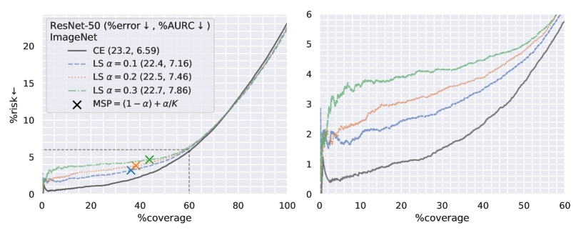
Figure 1: Risk$\downarrow$ (%error of accepted samples) vs coverage$\uparrow$ (proportion of samples accepted) plot showing selective classification (SC) performance for ResNet-50 trained on ImageNet-1k varying only $\alpha$, the level of label smoothing (LS). LS degrades SC performance, increasing the area under the curve, even though it improves the error rate at 100% coverage. LS seriously damages coverage at lower risk, which would particularly affect applications with low-risk tolerances.

Recent large-scale empirical evaluations of pre-trained models [20, 4] have shown that many strong classifiers have surprisingly poor SC ability. That is to say, in spite of having very low error rates, they are poor at rejecting their own misclassifications. Unfortunately, by evaluating pre-trained models from open-source repositories, the authors find it difficult to disentangle any potential causes of this behaviour, as model training recipes vary wildly from checkpoint to checkpoint. In this work, we reveal that label smoothing is one such potential cause and present the following key contributions:

1. We show empirically, across a range of network architectures and vision tasks, that training with LS consistently leads to degraded SC performance, even if it may improve accuracy (see Fig. 1). As LS can be found in the training recipes of many of the models evaluated in [20, 4], this suggests LS as one potential cause for previously unexplained negative results where strong classifiers underperform at SC.

2. We are able to explain the above behaviour by analysing the logit-level gradients of the LS loss. We show that the amount LS regularises the max logit directly corresponds to the true probability of error $P_{\text{error}}$, with regularisation increasing as $P_{\text{error}}$ decreases. This exacerbates overconfidence and underconfidence, degrading SC.

3. Finally, we demonstrate that logit normalisation proposed by Cattelan and Silva [4] is highly empirically effective in combating specifically the degradation caused by LS. Moreover, we are able to explain the effectiveness of logit normalisation through the lens of our gradient-based analysis, showing that normalisation compensates for the imbalanced regularisation by increasing uncertainty as the max logit increases.

2 Preliminaries

Consider a $K$-class neural network classifier with parameters $\boldsymbol{\theta}$ that models the conditional distribution $P(y|\boldsymbol{x};\boldsymbol{\theta})$ of labels $y\in\mathcal{Y}=\{\omega_{k}\}_{k=1}^{K}$ given inputs $\boldsymbol{x}\in\mathcal{X}=\mathbb{R}^{D}$. Typically the network has a categorical softmax output $\boldsymbol{\pi}(\boldsymbol{x};\boldsymbol{\theta})\in[0,1]^{K}$,

$$P(\omega_{k}|\boldsymbol{x};\boldsymbol{\theta})=\pi_{k}(\boldsymbol{x};\boldsymbol{\theta})=\exp v_{k}(\boldsymbol{x})/\sum_{i=1}^{K}\exp v_{i}(\boldsymbol{x})~{},\quad\boldsymbol{v}=\boldsymbol{W}\boldsymbol{z}+\boldsymbol{b}~{},$$ (1)

where $\boldsymbol{v}\in\mathbb{R}^{K}$ are the logits output by the final layer with weight matrix $\boldsymbol{W}\in\mathbb{R}^{K\times L}$, bias $\boldsymbol{b}\in\mathbb{R}^{K}$, and pre-logit features $\boldsymbol{z}\in\mathbb{R}^{L}$ as inputs. The classifier is trained by minimising the cross entropy (CE) loss on a finite dataset $\mathcal{D}_{\text{tr}}=\{x^{(n)},y^{(n)}\}_{n=1}^{N}$ drawn from distribution $p_{\text{data}}(\boldsymbol{x},y)$, such that it approximately learns the true conditional $P_{\text{data}}(y|\boldsymbol{x})$

$$\mathcal{L}_{\text{CE}}(\boldsymbol{\theta}) =-\frac{1}{N}\sum_{n}\sum_{k}\delta_{y^{(n)}\omega_{k}}\log P(\omega_{k}|\boldsymbol{x}^{(n)};\boldsymbol{\theta})$$ (2)

$$\approx-\mathbb{E}_{p_{\text{data}}(\boldsymbol{x})}\biggl{[}\sum_{k}P_{\text{data}}(\omega_{k}|\boldsymbol{x})\log P(\omega_{k}|\boldsymbol{x};\boldsymbol{\theta})\biggr{]}$$ (3)

$$=\mathbb{E}_{p_{\text{data}}(\boldsymbol{x})}\left[\text{KL}\left[\bar{\boldsymbol{\pi}}(\boldsymbol{x})||\boldsymbol{\pi}(\boldsymbol{x};\boldsymbol{\theta})\right]\right]+\text{const.}~{}=\mathcal{L}_{\text{CE}}^{\text{true}}(\boldsymbol{\theta})~{},$$ (4)

where $\delta$ is the Kronecker delta and KL$[\cdot||\cdot]$ is the Kullback–Leibler divergence. We use $\bar{\boldsymbol{\pi}}(\boldsymbol{x})\in[0,1]^{K}$ as a shorthand for the true conditional categorical, i.e. $\bar{\pi}_{k}=P_{\text{data}}(\omega_{k}|\boldsymbol{x})$. Predictions $\hat{y}$ are then made on new unlabelled input data $\boldsymbol{x}^{*}$ using classifier function $f$,

$$\hat{y}=f(\boldsymbol{x}^{*};\boldsymbol{\theta})=\operatorname*{arg\,max}_{\omega}P(\omega|\boldsymbol{x}^{*};\boldsymbol{\theta})~{}.$$ (5)

We also define the probability of the classifier making an error as,

$$P_{\text{error}}=1-\bar{\pi}_{\hat{y}}~{},$$ (6)

where, in a slight abuse of notation $\bar{\pi}_{\hat{y}}$ is the true probability of the predicted class.

2.1 Label Smoothing (LS)

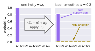
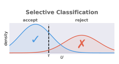
Figure 2: Left: illustration of how label smoothing (LS) alters a training label. LS reduces data supervision and adds regularisation. Right: illustration of selective classification (SC). Uncertain samples ($U>\tau$) are rejected, with the aim of reducing the number of errors ✗ served.

Label smoothing is most commonly understood (and implemented) as mixing the original one-hot labels (represented by $\delta$ in Eq. 2) with a uniform categorical distribution $\boldsymbol{u}=\boldsymbol{1}/K$ using hyperparameter $\alpha\in[0,1]$ (see Fig. 2). The label smoothing loss is thus

$$\mathcal{L}_{\text{LS}}(\boldsymbol{\theta};\alpha) =-\frac{1}{N}\sum_{n}\sum_{k}\left[(1-\alpha)\delta_{y^{(n)}\omega_{k}}+\alpha\frac{1}{K}\right]\log P(\omega_{k}|\boldsymbol{x}^{(n)};\boldsymbol{\theta})$$ (7)

$$=(1-\alpha)\mathcal{L}_{\text{CE}}(\boldsymbol{\theta})+\alpha\frac{1}{N}\sum_{n}\left[\text{KL}\left[\boldsymbol{u}||\boldsymbol{\pi}(\boldsymbol{x}^{(n)};\boldsymbol{\theta})\right]\right]+\text{const.}~{}$$ (8)

$$\approx\mathbb{E}_{p_{\text{data}}(\boldsymbol{x})}\Bigl{[}\text{KL}\Bigl{[}\underbrace{(1-\alpha)\bar{\boldsymbol{\pi}}(\boldsymbol{x})}_{\text{{\color[rgb]{0.58203125,0.41796875,0.9296875}data supervision}}}\,\,+\!\!\!\!\underbrace{\alpha\boldsymbol{u}}_{\text{{\color[rgb]{0.61328125,0.5,0.0234375}regularisation}}}\!\!\!\!||\boldsymbol{\pi}(\boldsymbol{x};\boldsymbol{\theta})\Bigr{]}\Bigr{]}+\text{const.}=\mathcal{L}_{\text{LS}}^{\text{true}}(\boldsymbol{\theta};\alpha)~{},$$ (9)

where we see that it can also be viewed as reduced CE supervision from the data combined with a regularisation term encouraging the softmax $\boldsymbol{\pi}$ to be uniform and preventing it from overfitting to the training data (Fig. 2). Eq. 9 also shows that LS can be seen as learning to predict a “softened” version of the true conditional $(1-\alpha)\bar{\boldsymbol{\pi}}(\boldsymbol{x})+\alpha\boldsymbol{u}$.

2.2 Selective Classification (SC)

A simple downstream task for estimates of predictive uncertainty is to reject (or detect) predictions that may incur a high cost [36, 81], using a binary rejection function,

$$g(\boldsymbol{x};\tau)=\begin{cases}0\text{ (reject prediction)},&\text{if }U(\boldsymbol{x})>\tau\text{ (uncertain)}\\ 1\text{ (accept prediction)},&\text{if }U(\boldsymbol{x})\leq\tau\text{ (confident)}~{},\end{cases}$$ (10)

where $U(\boldsymbol{x})$ is a scalar measure of predictive uncertainty extracted from the prediction model and $\tau$ is the operating threshold. Intuitively, we reject if the model is uncertain. Notably, we are only concerned with the relative rankings of $U$s rather than the absolute values. This differs from model calibration [25, 36], where the value of uncertainty predicted should match the marginal error rate over the data distribution for that value.

In the case where the prediction task is classification and we wish to reject potential misclassifications (✗), we can use a selective classifier [14, 9] $(f,g)$, which is simply the combination of a classifier $f$ (Eq. 5) and the aforementioned binary rejection function $g$ (Eq. 10). Fig. 2 contains an illustration. Given the 0/1 classification error,

$$\mathcal{L}_{\text{SC}}(f(\boldsymbol{x}),y)=\begin{cases}0,&\text{if }f(\boldsymbol{x})=y\quad\text{(correct {\color[rgb]{0.30859375,0.61328125,0.890625}\char 51})}\\ 1,&\text{if }f(\boldsymbol{x})\neq y\quad\text{(misclassified {\color[rgb]{0.890625,0.3984375,0.30859375}\char 55})}~{},\end{cases}$$ (11)

we define the selective risk [14, 22] as

$$\text{Risk}(f,g;\tau)=\frac{\mathbb{E}_{p_{\text{data}}(\boldsymbol{x},y)}[g(\boldsymbol{x};\tau)\mathcal{L}_{\text{SC}}(f(\boldsymbol{x}),y)]}{\mathbb{E}_{p_{\text{data}}(\boldsymbol{x},y)}[g(\boldsymbol{x};\tau)]}~{},$$ (12)

which is the average error on the accepted samples. The denominator of Eq. 12 is the proportion of samples accepted, or the coverage, $\text{Cov}=\mathbb{E}_{p_{\text{data}}(\boldsymbol{x})}[g(\boldsymbol{x};\tau)]$. Our objective is to minimise risk for a given coverage (lower %error on accepted samples) and/or maximise coverage for a given risk (accept more samples). Note this can be achieved both through improving $f$ (fewer errors) and through improving $g$ (better rejection). SC performance is evaluated via the Risk-Coverage (RC) curve [22] (Fig. 1 has an example). The area under the curve (AURC$\downarrow$) provides an aggregate metric over $\tau$, whilst the curve can also be inspected at specific operating points [78, 83], e.g. coverage at 5% risk (Cov@5$\uparrow$). For deployment, $\tau$ can be set using a held-out validation dataset by finding a suitable operating point on the RC curve according to an external requirement e.g. risk$=$5%.

$$U(\boldsymbol{x})=-\text{MSP}(\boldsymbol{x})=-\pi_{\text{max}}=-\max_{k}\pi_{k}(\boldsymbol{x};\theta)=-P(\hat{y}|\boldsymbol{x};\boldsymbol{\theta})~{},$$ (13)

i.e. the (negative of the) Maximum Softmax Probability (MSP) [30] is the model’s estimate of the probability of its prediction $\hat{y}$. We focus on this uncertainty measure $U$ for SC as it is a popular default choice and has been shown to consistently and reliably perform well in the literature [64, 81, 83, 36, 4, 15, 38, 22, 30].

2.2.1 Overconfidence.

Since we are only concerned about the rank ordering of uncertainties $U$, we loosely refer to overconfidence as when a model’s estimate of uncertainty is (relatively) low when $P_{\text{error}}$ high, as intuitively we would like a model to be uncertain when it is likely to be wrong. Underconfidence is then the inverse. Both will result in worse SC performance as overconfidence will cause errors to be accepted whilst underconfidence will lead to correct predictions being rejected. This is different to the more specific definition used in the problem scenario of model calibration [25].

2.3 Aleatoric and Epistemic Uncertainty

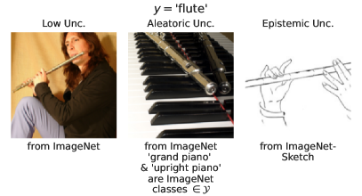
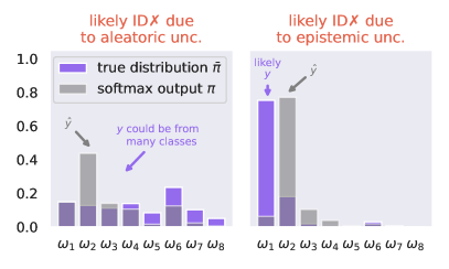
Figure 3: Left: different types of uncertainty for a model trained on ImageNet [63]. Aleatoric uncertainty is high as a different label $y$ could be sampled, while epistemic uncertainty is high as the image is from an unfamiliar domain, here ImageNet-Sketch [76]. Right: how errors arise from different uncertainties. Aleatoric uncertainty leads to errors as there are many probable labels. Epistemic uncertainty leads to errors as the model is unable to predict the true distribution $\bar{\boldsymbol{\pi}}$.

It is useful to separate uncertainty into two different types [39, 19, 35]. Aleatoric (or data) uncertainty is irreducible uncertainty in the data distribution $P_{\text{data}}(y|\boldsymbol{x})$, e.g. when there are multiple valid labels. Epistemic (or knowledge) uncertainty arises from a model’s lack of knowledge about data. A model should have greater epistemic uncertainty on the tails or low-density regions of $p_{\text{data}}(\boldsymbol{x})$, as these regions of the data distribution will be weighted less in the training loss (Eq. 4). There will also be epistemic uncertainty for different images not in training data, or images from a different domain. These different uncertainties are illustrated visually in Fig. 3 (left). While errors caused by aleatoric uncertainty are unavoidable, those due to epistemic uncertainty arise from the model’s inability to accurately predict the true conditional distribution $\bar{\boldsymbol{\pi}}$. These can be avoided with additional supervision. Both types of errors are illustrated in Fig. 3 (right). Epistemic uncertainty also intuitively results in both overconfidence and underconfidence. As the neural network models the data less accurately, its uncertainty estimates also more poorly reflect $P_{\text{error}}$ (both cases in Fig. 3 (right) are overconfident).

2.4 Experimental Details

We investigate large-scale image classification on ImageNet-1k [63] and semantic segmentation (pixel-level classification) on Cityscapes [12]. For ImageNet, we evaluate on the original validation set and randomly split 50,000 images from the training set for validation. For Cityscapes, we randomly split the original validation set into 100 validation and 400 evaluation images. To estimate the risk, we extract the model output prior to the final interpolation and subsample 5000 labelled pixels per image at random. We evaluate on the same pixels between models. All experiments are performed in Pytorch [61] and we will release our code shortly.

2.4.1 Models and Training

The only parameter varied between training runs is the level of label smoothing $\alpha$. Moreover, in order to isolate the effects of label smoothing, we train all our models from scratch using simple recipes. We purposely avoid popular augmentations such as MixUp [87] and CutMix [86] as these directly affect the training labels, which would interfere with our experiments. For image classification, we train ResNet-50 [27] and ViT-S-16 [13] on ImageNet-1k [63] using only random resized cropping and flipping for data augmentation. To achieve decent accuracy for ViT training from scratch without advanced augmentations, we use sharpness-aware minimisation (SAM) [16, 8]. For semantic segmentation, we train DeepLabV3+ [7] (ResNet-101 backbone) on Cityscapes [12]. We only use random cropping, flipping and colour jitter for augmentations. Full training details for reproducing our results can be found in the Appendix 0.B.

3 Label Smoothing Degrades Selective Classification Performance

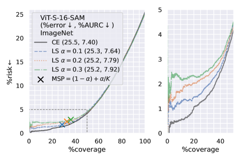
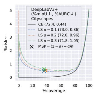
Figure 4: Risk-coverage plots for ViT-S-16-SAM trained on ImageNet-1k and DeepLabV3+ (ResNet-101) trained on Cityscapes, for different levels of LS $\alpha$. Although LS may improve error rate at 100% coverage, increasing $\alpha$ consistently degrades selective classification performance.

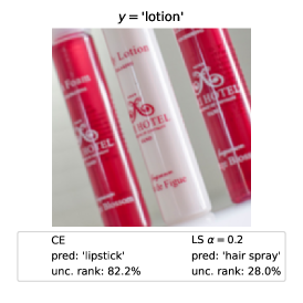
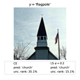
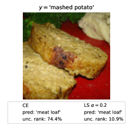
Figure 5: A few illustrative examples of overconfident errors performed by our LS-trained ResNet-50. Even though $P_{\text{error}}$ is high in all cases the model has predicted low-ranking (amongst all samples) uncertainty. Note that even though the CE model is wrong as well, it has assigned higher ranking uncertainties, reflecting its superior SC ability shown in Fig. 1. As an aside we note the high aleatoric uncertainty in ImageNet, arising from images containing multiple possible labels.

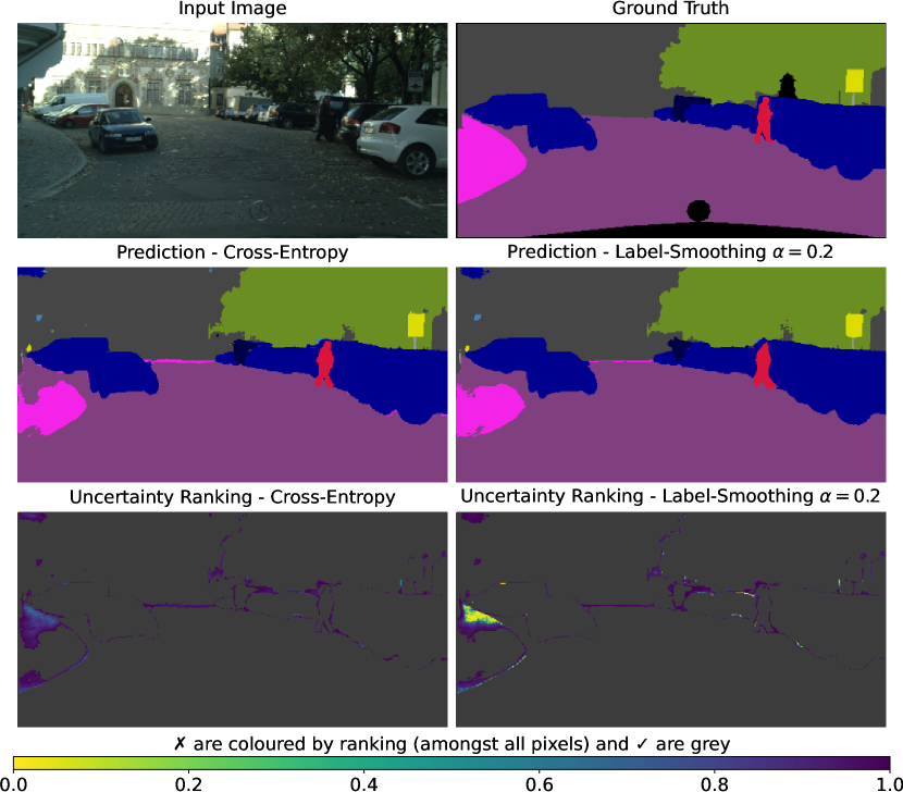
Figure 6: Visualisation of the overconfidence of DeepLabV3+ (ResNet-101) when trained using LS. We see that compared to the model trained using CE, the LS model predicts much lower uncertainty on incorrect ✗ segmentations. In particular, for the erroneous region on the left where the model has predicted parts of the “sidewalk” as “road”, the LS model is highly overconfident. This could have dire consequences in a safety-critical application such as autonomous driving.

Recently, large-scale empirical evaluations of SC for pre-trained models from open-source repositories [20, 4] have revealed that many strong classifiers surprisingly underperform on SC. In this section, we present LS as one possible cause of these previously unexplained results, and explain how LS may affect a model’s ability to perform SC.

To examine the effects of LS on SC performance, we plot RC curves for different architectures and tasks in Figs. 1 and 4. We use $U=-\text{MSP}$ and vary only the LS level $\alpha$ between training runs. We see that training with LS leads to a noticeable degradation for selective classification, despite improvements in top-1 error rate (risk at 100% coverage). That is to say, LS weakens the MSP score’s ability to differentiate ✓ vs ✗. We provide illustrative examples of this overconfidence on ImageNet in Fig. 5. The degradation in performance is especially evident for the low-risk regime, which is relevant to safety-critical scenarios where tolerances for error are low. For example, if the target is to achieve only 1% error on ImageNet, then none of our LS models are able to achieve a meaningful level of coverage, effectively not being able to serve any predictions.

To further highlight the overconfidence caused by LS, we visualise the uncertainty ranking of incorrect pixels for the segmentation of a Cityscapes scene in Fig. 6. We see that the LS-trained model is extremely confident for an erroneous region where it has predicted the “sidewalk” as “road”. Whilst the CE-trained model has made the same error, it is much more uncertain. This illustrates potential danger in an autonomous driving scenario if the vehicle is making decisions based on uncertainty estimates.

Upon inspection, many of the underperforming models benchmarked in [20, 4] are indeed trained using LS, further supporting our own results. The models are sourced from repositories such as from torchvision [61] and timm [79], where the original training recipes are mainly optimised for top-1 accuracy. We note that in the case of ImageNet, LS is such a common technique that it is often used by default, and not even mentioned in papers, e.g. [72, 73]. Overall, our results highlight that blindly optimising for accuracy may result in negative downstream consequences and that practitioners of selective classification need to be aware of the effects of their training recipes.

3.1 Considering Overconfidence Arising from Epistemic Uncertainty

It might intuitively seem odd that LS leads to such degraded SC performance since the transform applied to the true targets in Eq. 9 $(1-\alpha)\bar{\boldsymbol{\pi}}(\boldsymbol{x})+\boldsymbol{u}$ does not change the relative ranking of the maximum probability. However, this is only true for low epistemic uncertainty, i.e., when the model is knowledgeable about the data, so $\boldsymbol{\pi}(\boldsymbol{x};\boldsymbol{\theta})\approx(1-\alpha)\bar{\boldsymbol{\pi}}(\boldsymbol{x})+\boldsymbol{u}$. For such samples, the model has learnt to be more uncertain. However, we cannot assume that epistemic uncertainty is always low. Moreover, we know it leads to both errors and overconfidence (Fig. 3 (right)). One clue that points to epistemic uncertainty is the fact that for the LS-trained models, Figs. 1 and 4 show that many samples have $\pi_{\text{max}}>(1-\alpha)+\alpha/K$, and it is for these such samples that SC performance is degraded the most. As the training targets never exceed $(1-\alpha)+\alpha/K$, this inaccuracy in predicting the smoothed targets could be due to epistemic uncertainty.

3.2 Comparing Logit Gradients Between CE and LS

To better understand how LS could lead to the poor SC performance exhibited in the RC curves of Figs. 1 and 4, we consider how LS affects logit-level training gradients. These are the first term in the chain rule for backpropagation and so directly contribute to all parameter gradients during training. We take the gradient of $\mathcal{L}^{\text{true}}$ (Eqs. 4 and 9), which the empirical loss approximates, for a single sample,

$$\frac{\partial\mathcal{L}_{\text{CE}}^{\text{true}}}{\partial v_{k}}=-\left[\bar{\pi}_{k}\!\!-\pi_{k}\right],\quad\frac{\partial\mathcal{L}_{\text{LS}}^{\text{true}}}{\partial v_{k}}=-\biggl{[}\Bigl{[}\,\underbrace{(1-\alpha)\bar{\pi}_{k}}_{\text{{\color[rgb]{0.58203125,0.41796875,0.9296875}data supervision}}}+\!\!\!\!\underbrace{\alpha/K}_{\text{{\color[rgb]{0.61328125,0.5,0.0234375}regularisation}}}\!\!\!\!\Bigr{]}\!-\pi_{k}\biggr{]},$$ (14)

where in a slight abuse of notation we omit the outer expectation over $p_{\text{data}}(\boldsymbol{x})$ for convenience. We can then define the regularisation gradient on the logits,

$$\frac{\partial\mathcal{L}^{\text{true}}_{\text{reg}}}{\partial v_{k}}=\frac{\partial(\mathcal{L}_{\text{LS}}^{\text{true}}-\mathcal{L}_{\text{CE}}^{\text{true}})}{\partial v_{k}}=\frac{\mathcal{L}_{\text{LS}}^{\text{true}}}{\partial v_{k}}-\frac{\mathcal{L}_{\text{CE}}^{\text{true}}}{\partial v_{k}}=\alpha\left[\bar{\pi}_{k}-1/K\right]=\alpha\bar{\pi}_{k}-\alpha/K~{},$$ (15)

which is the difference between the LS and CE gradients. This intuitively represents how LS regularises training at the logit level in comparison to CE. Crucially, it only depends on the true distribution $\bar{\boldsymbol{\pi}}$. Gradient descent involves updating weights in the opposite direction to the gradient. Hence $\alpha\bar{\pi}_{k}$ penalises $v_{k}$ when the true probability $\bar{\pi}_{k}$ is higher. The second term $-\alpha/K$ uniformly increases the logits. This does not affect the softmax output as it is invariant to uniform logit shifts $\boldsymbol{\pi}(\boldsymbol{v})=\boldsymbol{\pi}(\boldsymbol{v}+\eta\boldsymbol{1})$, $\eta\in\mathbb{R}$ [44].

3.3 Label Smoothing Exacerbates Overconfidence and Underconfidence

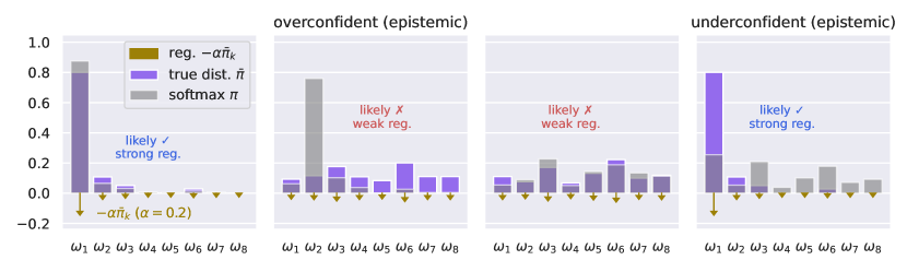
Figure 7: Illustration of how the regularisation gradient (Eq. 15), which is the difference between LS and CE gradients, affects the logits differently. When $U$ is lower (sharper softmax), the regularisation on the max logit is lower when epistemic uncertainty has caused overconfidence. When $U$ is higher (flatter softmax), the regularisation is higher when epistemic uncertainty has caused underconfidence. Thus, LS exacerbates both of these issues, degrading the rank ordering of $U$ and diminishing the ability of the softmax to differentiate correct ✓ from incorrect ✗ .

We now consider how the regularisation gradient affects the maximum logit,

$$\frac{\partial\mathcal{L}^{\text{true}}_{\text{reg}}}{\partial v_{\text{max}}}=\alpha\bar{\pi}_{\hat{y}}-\alpha/K=\alpha[1-P_{\text{error}}]-\alpha/K,$$ (16)

which shows that the regularisation on $v_{\text{max}}$ decreases as the probability of error increases. This directly impacts softmax-based uncertainties, especially for lower uncertainties where $v_{\text{max}}$ will dominate the softmax. Eq. 16 means that for predictions that share the same value of $U$, those with higher $P_{\text{error}}$ (more likely ✗), will have $v_{\text{max}}$ regularised less, whilst predictions with lower $P_{\text{error}}$ (more likely ✓) will have $v_{\text{max}}$ regularised more. Thus, softmax-based uncertainties will have the relative ranking of correct ✓ and incorrect ✗ predictions degraded, harming selective classification.

To further build an intuition, we consider overconfidence and underconfidence as a result of epistemic uncertainty. As illustrated in Fig. 7, when $U$ is low, and a model is overconfident due to epistemic uncertainty (i.e. $P_{\text{error}}$ is high), the regularisation gradient is much weaker compared to when $P_{\text{error}}$ is low for the same $U$. On the other hand, when $U$ is high and a model is underconfident due to epistemic uncertainty (i.e. $P_{\text{error}}$ is low), the regularisation gradient is much stronger compared to when $P_{\text{error}}$ is high for the same $U$. Thus, both overconfidence and underconfidence are exacerbated by label smoothing, degrading the model’s ability to perform selective classification.

To test our analysis, we artificially inject epistemic uncertainty into our ImageNet evaluation using ImageNet-Sketch [76], a dataset containing sketches of each ImageNet class (see Fig. 3 for an example). We combine the 50,889 ImageNet-Sketch images with the 50,000 ImageNet evaluation images and plot the new risk vs coverage for all 100,889 samples in Fig. 8. We find that even though the regularisation of LS still improves the error rate, the degradation in SC from LS is exacerbated at lower coverages, where the CE-trained model maintains much lower risk. At 10% coverage of the combined evaluation set, LS leads to accepting many more errors compared to CE, with an increasing proportion originating from ImageNet-Sketch. This demonstrates that LS exacerbates overconfidence arising from epistemic uncertainty, reducing a model’s ability to reject errors.

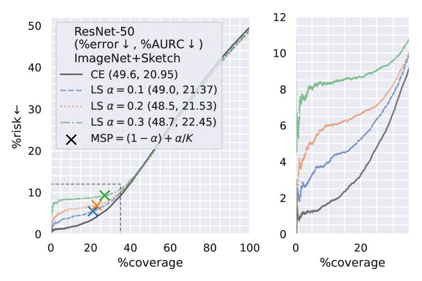
	@10% coverage of ImageNet + Sketch
		ImageNet	Sketch
CE	#samples	8994	1094
	#errors	93	80
	error rate	1.0	7.3
LS $\alpha=0.1$	#samples	8561	1527
	#errors	187	211
	error rate	2.2	13.8
LS $\alpha=0.2$	#samples	8171	1917
	#errors	244	365
	error rate	3.0	19.0
LS $\alpha=0.3$	#samples	7915	2173
	#errors	297	541
	error rate	3.8	24.9

Figure 8: Left: RC curve for ResNet-50 when evaluation is on the combination of ImageNet and ImageNet-sketch (ViT-S-16 can be found in Appendix 0.A). We see that for low-uncertainty predictions, the degradation caused by LS is exacerbated when epistemic uncertainty is artificially introduced. Right: statistics @10% coverage of the combined evaluation set. As the level of LS $\alpha$ increases, the number of errors increases, especially the number of errors from ImageNet-Sketch. This shows that LS exacerbates model overconfidence arising from epistemic uncertainty.

4 Logit Normalisation Improves the SC of LS-Trained Models

Ideally, we would like to find a way to recover from the degradation caused by LS. A recent study by Cattelan and Silva [4] has shown that logit normalisation can improve the SC performance of many pre-trained models. The logits are normalised by their $p$-norm and then the MSP score $\pi_{\text{max}}$ is replaced by the normalised max logit

$$U=-v^{\prime}_{\text{max}},\quad\boldsymbol{v}^{\prime}=\frac{\boldsymbol{v}}{\left\lVert\boldsymbol{v}\right\rVert_{p}}=\boldsymbol{v}/\bigl{(}\sum_{k}v_{k}^{p}\bigr{)}^{\frac{1}{p}}~{},$$ (17)

where $p$ is found via grid search on a validation set. We investigate the efficacy of this approach, applying it to our LS-trained models. Fig. 9 (left) shows the SC performance with and without logit normalisation, and we indeed find that applying logit normalisation greatly improves SC performance for models trained using LS, allowing for improved error rate (@100% coverage) without compromising on SC. This is further visualised for semantic segmentation in Fig. 10, where logit normalisation successfully mitigates the previously observed overconfidence caused by LS. However, we also find that logit normalisation does not notably improve the ability of CE-trained models. This aligns with the results reported [4] where certain models do not benefit from logit normalisation so the authors suggest “falling back” to the MSP.

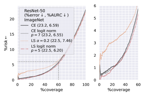
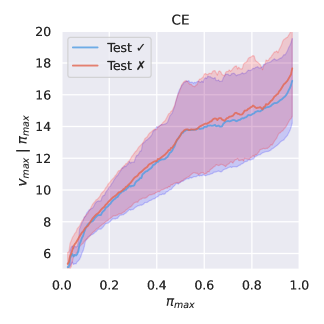
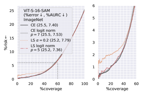
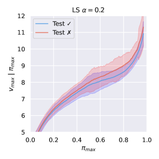
Figure 9: Left: RC curves showing the effect of logit normalisation. Logit normalisation improves SC performance on LS-trained models, but has little effect on CE-trained models. DeepLabV3+ can be found in Appendix 0.A. Right: distribution of the max logit $v_{\text{max}}$ given the MSP $\pi_{\text{max}}$ for correct ✓ and incorrect ✗ predictions separately. We see that $v_{\text{max}}$ is higher for ✗ for the LS-trained model, whilst the distributions are roughly the same for CE. This matches the max logit regularisation described in Eq. 16. We calculate the mean$\pm$std. in a 0.05-wide sliding window.

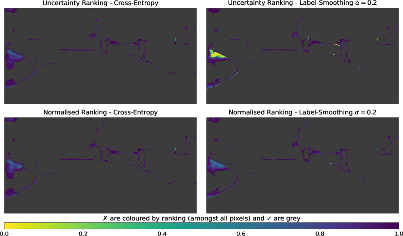
Figure 10: Visualisation of the effect of logit normalisation for semantic segmentation (same scene as Fig. 6). Logit normalisation significantly reduces the overconfidence of the LS-trained model, although it has little effect on the uncertainty of the CE-trained model.

4.1 Explaining the Effectiveness of Logit Normalisation.

Although Cattelan and Silva [4] validate this approach on a large number of pre-trained models, they provide little explanation as to why it is so effective (or indeed why it isn’t effective sometimes). Let us highlight the interaction between logit normalisation and label smoothing. If we examine Eq. 17, we see that it resembles the softmax. However, in this case, the logits are raised to power $p$ rather than being exponentiated. Crucially, whilst the softmax is invariant to uniform shifts in the logits,

$$\pi_{k}(\boldsymbol{v})=\frac{\exp v_{k}}{\sum_{i}\exp v_{i}}=\frac{\exp(v_{k}+\eta)}{\sum_{i}\exp(v_{i}+\eta)}=\pi_{k}(\boldsymbol{v}+\eta\boldsymbol{1}),\quad\forall\eta\in\mathbb{R}~{},$$ (18)

this is not the case for $\boldsymbol{v}^{\prime}$. In fact, we have the following inequality for positive logits $\boldsymbol{v}$:

Result 1.

For all strictly positive vectors $\boldsymbol{v}\in\left(\mathbb{R}_{>0}\right)^{K}$, containing at least two different values, and $p\in[1,+\infty[$, the ratio of the $\infty$-norm and the $p$-norm strictly decreases when summing $v$ with any uniform vector $\eta\boldsymbol{1}$, $\eta$ strictly positive:

$$\frac{||\boldsymbol{v}||_{\infty}}{||\boldsymbol{v}||_{p}}>\frac{||\boldsymbol{v}+\eta\boldsymbol{1}||_{\infty}}{||\boldsymbol{v}+\eta\boldsymbol{1}||_{p}}~{}.$$ (19)

The proof can be found in Appendix 0.C. Recalling that $||\boldsymbol{v}||_{\infty}=v_{\text{max}}$, Result 1 thus implies that for a given softmax output $\boldsymbol{\pi}(\boldsymbol{v})=\boldsymbol{\pi}(\boldsymbol{v}+\eta\boldsymbol{1})$ and arbitrary corresponding $\boldsymbol{v}$, the greater the value of $\eta$ and thus $v_{\text{max}}$, the lower the value of $v^{\prime}_{\text{max}}$. That is to say logit normalisation increases the estimated uncertainty when the max logit $v_{\text{max}}$ is higher for the same softmax probabilities $\boldsymbol{\pi}$.

Recall that in Sec. 3.3 we found that the maximum logit $v_{\text{max}}$ is less regularised the more likely a prediction is wrong ✗, i.e. when $P_{\text{error}}$ is high (Eq. 16). We plot $v_{\text{max}}$ given the MSP, separately for correct ✓ and incorrect ✗ predictions in Fig. 9, and see an interesting behaviour emerge. For the model trained with LS, the imbalanced logit regularisation described in Eq. 16 has caused $v_{\text{max}}$ to become higher for misclassifications ✗ than correct predictions ✓, i.e. information about $P_{\text{error}}$ has been encoded in $v_{\text{max}}$.

As Result 1 says that for the same softmax output $\boldsymbol{\pi}$, $v^{\prime}_{\text{max}}$ will decrease as $v_{\text{max}}$ increases, logit normalisation will increase uncertainty when $v_{\text{max}}$ is higher, effectively reversing the effect of the imbalanced logit regularisation. This will then improve the rank ordering of the uncertainty score $U$ and thus improve the SC performance of the LS-trained model. Given our analysis and empirical results, we strongly recommend the use of logit normalisation for LS-trained models for performing selective classification.

On the other hand, Fig. 9 (right) also shows that the distributions of $v_{\text{max}}$ given $\pi_{\text{max}}$ for correct ✓ and incorrect ✗ predictions are very similar for the CE-trained model. This explains why, for the models trained using CE, logit-normalisation does not seem to help, as $v_{\text{max}}$ does not provide useful information about $P_{\text{error}}$ given $\pi_{\text{max}}$.

5 Related Work

5.0.1 Prediction with Rejection.

Selective classification falls into the broader problem setting of prediction with rejection. In the case of SC, misclassifications are to be rejected [14]. The baseline approach is to use the MSP [30, 22] and there have been a number of proposed training [57, 33, 89] and architectural [23, 11] enhancements, however, recently the effectiveness of some of these enhancements has been called into question [15]. In this work, we focus on only the MSP. Another scenario involving prediction with rejection is out-of-distribution (OOD) detection [84, 30], where data from outside of the training distribution are to be rejected. There is a plethora of varied research in this field [82, 68, 49, 88, 50, 34, 77, 29] extending to semantic segmentation [26, 46, 2, 24, 18]. Recently, a combination of SC and OOD detection has been proposed, where the aim is to reject both misclassifications and OOD data [36, 81, 38, 5]. Notably, Deep Ensembles [43] have arisen as a reliable method to improve performance in all three scenarios [38, 83, 45]. We believe, given the results of this work, that extending the investigation of LS (and other training enhancements) to other scenarios involving prediction with rejection is an important avenue of future work.

5.0.2 Mixup.

Mixup [87] and its variants [86, 17, 62, 54, 3] are a set of regularisation techniques that involve interpolating between random pairs of samples at training time, modifying both inputs and targets. They are commonly found in many ImageNet training recipes [73, 52, 51] and often used in conjunction with label smoothing [80, 74, 53]. We remark that research into how Mixup and its variants affect SC is a particularly salient avenue of future work as it similarly “softens” the classification training targets.

5.0.3 Label Smoothing.

Beyond prediction with rejection, label smoothing [70] is well investigated. It has been shown to improve model calibration [59, 58, 47, 10] as well as accuracy when training under label noise [56]. Knowledge distillation [31], where soft labels are provided by a teacher network, is also commonly linked and combined with LS [59, 21, 65, 6, 85] due to their similarity. Interestingly, in a similar vein to our work, pre-training using LS has been shown to harm transfer learning [40].

6 Concluding Remarks

In this work, we investigate the effect that label smoothing has on a model’s ability to perform selective classification. Our experiments across a range of architectures and tasks reveal that the use of label smoothing leads to consistent degradation in a model’s ability to reject misclassifications, even if it improves classification performance. By analysing the logit-level gradients of the label smoothing loss, we are able to explain this behaviour – label smoothing increasingly regularises the max logit as the true probability of error decreases, exacerbating overconfidence and underconfidence. We then investigate logit normalisation as a potential method to improve the degraded selective performance of label-smoothing-trained models. We find it to be highly effective, as it, in essence, reverses the effect of the aforementioned imbalanced regularisation by increasing the uncertainty when the max logit is higher. We hope that our work encourages more research into understanding how different training techniques may impact model performance in downstream applications such as uncertainty estimation.

6.0.1 Acknowledgments.

This work was performed using HPC resources from GENCI-IDRIS (Grant 2023-[AD011011970R3]). GX’s PhD is funded jointly by Arm and the EPSRC.

Understanding Why Label Smoothing
Degrades Selective Classification and How to Fix It
 
Supplementary Material

Appendix 0.A Additional Results

We include additional experimental results that mirror those found in the main paper on ResNet-50, for ViT-S-16 and DeepLabV3+:

• Fig. 11 shows ViT-S-16 evaluated on the combination of ImageNet and ImageNet-Sketch. The behaviour mirrors that of ResNet-50 in the main paper.

• Fig. 12 shows the effectiveness of logit normalisation on DeepLabV3+ (ResNet-101) on Cityscapes.

• Figs. 13 and 14 shows the distribution of $v_{\text{max}}$ given $\pi_{\text{max}}$ for ViT-S-16 and DeepLabV3+. We see that similarly to ResNet-50, for LS, the distribution of $v_{\text{max}}$ is higher for errors ✗. Although it is less obvious, it is clear for both ViT-S-16 and DeepLabV3+ that for higher $\pi_{\text{max}}$ the standard deviations overlap much less than for CE.

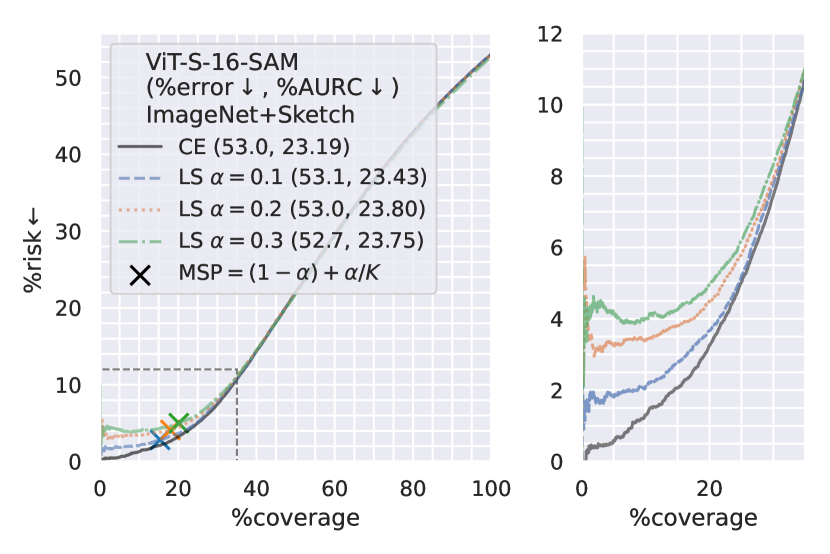
	@10% coverage of ImageNet + Sketch
		ImageNet	Sketch
CE	#samples	9528	560
	#errors	88	43
	error rate	0.9	7.7
LS $\alpha=0.1$	#samples	9332	756
	#errors	130	83
	error rate	1.4	11.0
LS $\alpha=0.2$	#samples	9117	971
	#errors	177	164
	error rate	1.9	16.9
LS $\alpha=0.3$	#samples	8966	1122
	#errors	208	195
	error rate	2.3	17.4

Figure 11: ViT-S-16 evaluated on the combination of ImageNet and ImageNet-Sketch. The results mirror ResNet-50 from the main paper. LS leads to increased overconfidence when epistemic uncertainty is introduced, as shown through the increase in the failure rate amongst high-confidence samples.

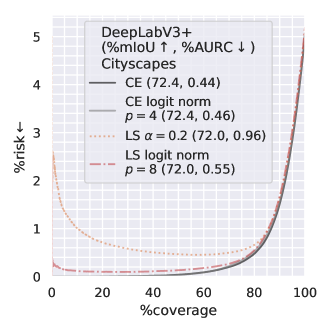
Figure 12: RC curve showing the effect of logit normalisation for DeepLabV3+ (ResNet-101). The behaviour is similar to the results in the main paper. Logit normalisation is effective in improving the performance of the LS-trained model, however, makes little difference to the CE-trained model.

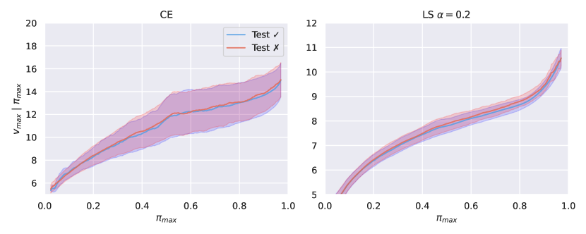
Figure 13: The max logit $v_{\text{max}}$ as a function of the MSP $\pi_{\text{max}}$ for correct ✓ and incorrect ✗ predictions separately for ViT-S-16. Similarly to the main paper, the distribution is higher for errors ✗ for the LS-trained model. We calculate the mean$\pm$std. in a 0.05-wide sliding window.

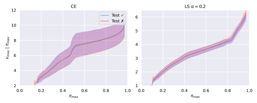
Figure 14: The same as Fig. 13 but for DeepLabV3+ (ResNet-101)

0.A.1 Small-Scale CIFAR Experiments

We also include experimental results on small-scale $32\times 32$ CIFAR-100 [41]. We train a DenseNet-BC [32] ($k=12,L=100$) to show further generality over model architecture families. Figs. 15, 16 and 17 show results that mirror those found in the main paper for ResNet-50 on ImageNet, although we note that LS does not improve top-1 error rate in this case.

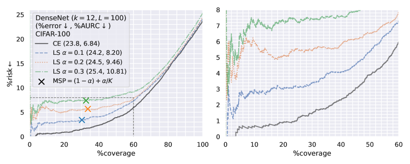
Figure 15: RC curves for DenseNet on CIFAR-100 – LS degrades SC

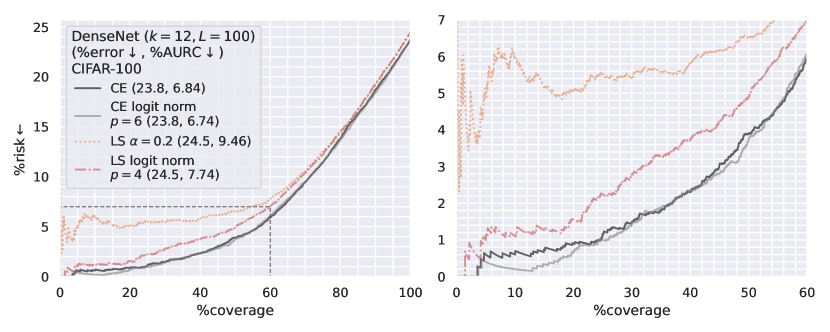
Figure 16: DenseNet on CIFAR-100 – logit normalisation improves SC for LS but not for CE

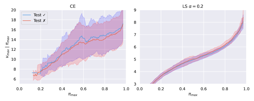
Figure 17: DenseNet on CIFAR-100 – LS leads to higher $v_{\text{max}}$ on errors ✗

Appendix 0.B Reproducibility

Alongside this document, we provide a code demo to train two ResNet-20 [27] on CIFAR-10 [41] with cross-entropy and label smoothing and compare the corresponding Risk-Coverage curves. We recall that all the code used in this project will be made available shortly to ensure exact reproducibility. We also plan to release our most important models on Hugging Face.

Here, we provide the full details of our training recipes used in the main paper and in the additional results presented in Appendix 0.A. All our models are trained with PyTorch, and we use the native implementation from the CrossEntropyLoss for label smoothing.

0.B.1 Image Classification

DenseNet – CIFAR100.

For the DenseNet trained on CIFAR-100, we extract a subset of CIFAR’s training set containing 5000 images to create a proper validation set. We take batches of 64 32$\times$32-pixel images and train on a single GPU for 300 epochs using stochastic gradient descent and a starting learning rate of 0.1, Nesterov [60, 69], a momentum of 0.9, and $1\times 10^{-4}$ weight decay. We divide the learning rate by ten after 150 and 225 epochs. We use standard augmentations. We apply random crop with a four-pixel padding as well as random horizontal flip. We do not perform model selection and keep the last checkpoint.

ViT-16-S – ImageNet.

For our ViT-16-S trained on ImageNet, we take batches of 2048 images and train on 8 V100 for 300 epochs with AdamW [55] with the $\beta$s equal to 0.9 and 0.999. We start with a linear warmup for 15 epochs, then use a cosine annealing scheduler with $3\times 10^{-3}$ as the starting learning rate. The models are trained with non-adaptive sharpness-aware minimisation (SAM) [16, 8] with $\rho=0.2$. We use a dropout [66] rate of 0.1 but no attention dropout. We transform the training images with a standard random resized crop to 224$\times$224 pixels using bicubic interpolation and a random horizontal flip. For evaluation, we center-crop the images to this resolution. For ImageNet, we do not perform model selection and keep the last checkpoint. However, we randomly extract a validation set of 50000 images from the training set to perform logit normalisation.

ResNet-50 – ImageNet.

Our ResNet-50 is trained on 8 V100 with stochastic gradient descent for 120 epochs using a batch size of 1024 images. After five epochs of linear warmup, we use a cosine annealing scheduler starting with a learning rate of 0.4 with a momentum of 0.9 and a weight decay of $1\times 10^{-4}$. We use the same transformation of the images as for the ViT and select the last checkpoint for inference. We use the same evaluation set as for the ViT for logit normalisation.

0.B.2 Semantic Segmentation

Deeplabv3+.

We train a Deeplabv3+ on CityScapes [12] with a ResNet-101 [27] backbone pre-trained on ImageNet [63]. We use stochastic gradient descent with a base learning rate of 0.01, divided by 10 for the backbone weights, and reduced following the "poly" policy [48] with a power of 0.9. The weights are optimised with a momentum of 0.9 and a weight decay of $10^{-4}$. We take a batch size of 12 images and train for 40000 steps. During training, we randomly crop the input images and targets to squares with 768-pixel-long sides. We apply random horizontal flip and colour-jitter with the classical parameters: brightness, contrast, and saturation levels of 0.5. For testing, we use the images at their original resolution and do not perform any test time augmentations. For the RC curves, we randomly sample 5000 predictions per image, extracted prior to the final interpolation to reduce correlations between the predictions. We keep the pixel-wise locations of the samples when changing the level of label smoothing $\alpha$ to ensure fair comparisons.

Appendix 0.C Result and Proof

Result.

For all strictly positive vectors $\boldsymbol{v}\in\left(\mathbb{R}_{>0}\right)^{K}$ containing at least two different values and $p\in[1,+\infty[$, the ratio of the infinite norm and the p-norm strictly decreases when summing $v$ and any uniform vector $\eta\boldsymbol{1}$, $\eta$ strictly positive:

$$\frac{||\boldsymbol{v}||_{\infty}}{||\boldsymbol{v}||_{p}}>\frac{||\boldsymbol{v}+\eta\boldsymbol{1}||_{\infty}}{||\boldsymbol{v}+\eta\boldsymbol{1}||_{p}}.$$ (20)

Proof.

Let there be a real $\eta>0$. Take $p\geq 1$ the dimension of the norm and $\boldsymbol{v}$ a vector of dimension $K\geq 1$ of strictly positive elements $v_{k}$ for $1\leq k\leq K$, such that there exists $1\leq i\leq K$ such that $v_{i}<\max\limits_{k\leq K}v_{k}$. We have that

$$1+\frac{\eta}{v_{k}}\geq 1+\frac{\eta}{\max\limits_{k\leq K}v_{k}},$$ (21)

and, for at least $i$, we have the same equation, yet with strict inequality. We can adapt Eq. 21 to get

$$v_{k}+\eta\geq\frac{\max\limits_{k\leq K}(v_{k}+\eta)}{\max\limits_{k\leq K}v_{k}}v_{k}.$$ (22)

And when set to exponent $p\geq 1$, we obtain

$$\frac{(v_{k}+\eta)^{p}}{\max\limits_{k\leq K}(v_{k}+\eta)^{p}}\geq\frac{v_{k}^{p}}{\max\limits_{k\leq K}v_{k}^{p}}.$$ (23)

As for Eq. 21, please note that using $k=i$, we get the same equation as Eq. 23, although with a strict inequality. We can now sum on the elements of $\boldsymbol{v}$ to get

$$\frac{\sum\limits_{k=1}^{K}(v_{k}+\eta)^{p}}{\max\limits_{k\leq K}(v_{k}+\eta)^{p}}>\frac{\sum\limits_{k=1}^{n}v_{k}^{p}}{\max\limits_{k\leq K}v_{k}^{p}}.$$ (24)

By taking the inverse, we get

$$\frac{\max\limits_{k\leq K}v_{k}^{p}}{\sum\limits_{k=1}^{n}v_{k}^{p}}>\frac{\max\limits_{k\leq K}(v_{k}+\eta)^{p}}{\sum\limits_{k=1}^{K}(v_{k}+\eta)^{p}}.$$ (25)

And setting the equation to the exponent $p^{-1}$ and replacing the maxima of the $v_{k}$ and $v_{k}+\eta$ with the infinite norm, $||\boldsymbol{v}||_{\infty}$ and $||\boldsymbol{v}+\eta\boldsymbol{1}||_{\infty}$ respectively, we obtain the result. ∎

Appendix 0.D Discussions

0.D.1 On the Assumption that Logits are Positive

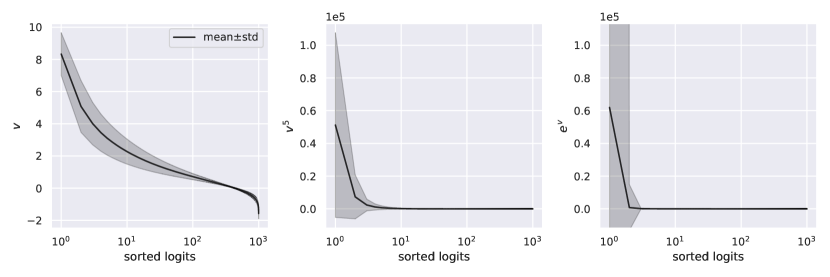
Figure 18: Mean$\pm$std after logits have been sorted highest to lowest for ResNet-50 $\alpha=0.2$ on the ImageNet evaluation set. We see that $v^{5}$ and $\exp v$ are much larger for the top $<10$ logits. Thus these logits dominate $\pi_{\text{max}}$ and $v^{\prime}_{\text{max}}$.

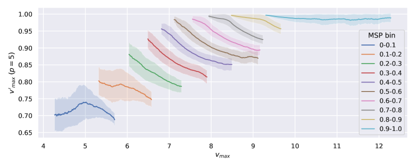
Figure 19: $v^{\prime}_{\text{max}}$ given $v_{\text{max}}$ within bins of similar MSP for ResNet-50 $\alpha=0.2$ on the ImageNet evaluation set. Generally, $v^{\prime}_{\text{max}}$ increases as $v_{\text{max}}$ decreases, showing empirically how logit normalisation increases uncertainty for higher $v_{\text{max}}$. We calculate the mean$\pm$std. of $v^{\prime}_{\text{max}}$ in a 0.2-wide sliding window for samples with $v_{\text{max}}$ within mean$\pm$2std of $v_{\text{max}}$ within the bin (to remove noisy averages).

Result 1 assumes that all elements in the logit vector are $>0$, which is not necessarily true. However, we also find empirically that both $v^{\prime}_{\text{max}}$ and $\pi_{\text{max}}$ tend to be dominated by the largest positive logits. This is intuitive as exponentiating or raising to power $p$ ($p\geq 4$ in our experiments) will amplify the larger logits. This is shown in Fig. 18, where we plot the mean$\pm$std of $v,v^{5}$ and $\exp v$ for the sorted logits of ResNet-50 $\alpha=0.2$ on the ImageNet evaluation set. Thus $\pi_{\text{max}}(\boldsymbol{v})\approx\pi_{\text{max}}(\boldsymbol{v}_{\text{top-}k})$ and $v^{\prime}_{\text{max}}(\boldsymbol{v})\approx v^{\prime}_{\text{max}}(\boldsymbol{v}_{\text{top-}k})$, where the top-$k$ logits are positive. As Result 1 holds for $v^{\prime}_{\text{max}}(\boldsymbol{v}_{\text{top-}k})$, we still expect logit normalisation to penalise higher $v_{\text{max}}$ when comparing samples with similar $\pi_{\text{max}}$.

We can consider the scenario where we add $\eta$ to only the top-$k$ logits. This more aptly describes the empirical logit behaviour compared to adding $\eta$ to all logits, as the values of the lower ranking logits vary much less than the higher ranking ones (Fig. 18). Here we would expect $\pi_{\text{max}}(\boldsymbol{v})$ to increase very slightly, but would expect $v^{\prime}_{\text{max}}(\boldsymbol{v})$ to decrease as the numerator of Eq. 24 would be dominated by the top-$k$ largest logits.

Fig. 19 shows how empirically logit normalisation indeed increases uncertainty for higher $v_{\text{max}}$. We plot the mean$\pm$std of $v^{\prime}_{\text{max}}$ given $v_{\text{max}}$ for samples in different MSP bins. We see clearly that in almost all cases, for samples with similar $\pi_{\text{max}}$, the normalised max logit $v^{\prime}_{\text{max}}$ increases as the original max logit $v_{\text{max}}$ decreases. As such, logit normalisation is able to improve the SC performance of LS-trained models.

0.D.2 Existing Benchmarks and Training Recipes

Although we do not exhaustively search all training recipes for all models benchmarked in [20, 4], we do provide a number of examples of evaluated models trained with label smoothing. We also provide links to publicly available training repositories, as not all papers mention label smoothing even when it is used in training. Upon inspection of [20, 4], these models do in fact seem to underperform at selective classification (and Cattelan and Silva [4] report that their AURCs benefit from logit normalisation).

• EfficientNet [72]: https://github.com/tensorflow/tpu/blob/master/models/official/efficientnet/main.py#L249

• EfficientNet-V2 [73]: https://github.com/google/automl/blob/master/efficientnetv2/datasets.py#L658

• DeiT [74]: https://github.com/facebookresearch/deit/blob/main/main.py#L101

• Swin-Transformer (+V2) [51, 52]:
  https://github.com/microsoft/Swin-Transformer/blob/main/config.py#L70

• ConvNeXt [53]: https://github.com/facebookresearch/ConvNeXt/blob/main/main.py#L105

• Torchvision [61] (various): https://github.com/pytorch/vision/tree/main/references/classification

Galil et al. [20] state that some of their best performing ViT models [13, 67, 8] are trained with label smoothing (their Tab.1). However, after inspecting both the original papers and open-source repositories of the aforementioned work we were unable to find any confirmation of the use of label smoothing.

References

- Beam and Kompa [2021] Beam, A., Kompa, B.: Second opinion needed: Communicating uncertainty in medical artificial intelligence. NPJ Digital Medicine (2021)
- Besnier et al. [2021] Besnier, V., Bursuc, A., Picard, D., Briot, A.: Triggering failures: Out-of-distribution detection by learning from local adversarial attacks in semantic segmentation. In: ICCV (2021)
- Bouniot et al. [2023] Bouniot, Q., Mozharovskyi, P., d’Alché Buc, F.: Tailoring mixup to data using kernel warping functions. arXiv preprint arXiv:2311.01434 (2023)
- Cattelan and Silva [2023] Cattelan, L.F.P., Silva, D.: How to fix a broken confidence estimator: Evaluating post-hoc methods for selective classification with deep neural networks. ArXiv abs/2305.15508 (2023)
- CEN et al. [2023] CEN, J., Luan, D., Zhang, S., Pei, Y., Zhang, Y., Zhao, D., Shen, S., Chen, Q.: The devil is in the wrongly-classified samples: Towards unified open-set recognition. In: ICLR (2023)
- Chandrasegaran et al. [2022] Chandrasegaran, K., Tran, N.T., Zhao, Y., Cheung, N.M.: Revisiting label smoothing and knowledge distillation compatibility: What was missing? In: ICML (2022)
- Chen et al. [2018] Chen, L.C., Zhu, Y., Papandreou, G., Schroff, F., Adam, H.: Encoder-decoder with atrous separable convolution for semantic image segmentation. In: ECCV (2018)
- Chen et al. [2022] Chen, X., Hsieh, C.J., Gong, B.: When vision transformers outperform resnets without pre-training or strong data augmentations. In: ICLR (2022)
- Chow [1957] Chow, C.K.: An optimum character recognition system using decision functions. IRE Transactions on Electronic Computers (1957)
- Chun et al. [2020] Chun, S., Oh, S.J., Yun, S., Han, D., Choe, J., Yoo, Y.J.: An empirical evaluation on robustness and uncertainty of regularization methods. ArXiv abs/2003.03879 (2020)
- Corbière et al. [2019] Corbière, C., Thome, N., Bar-Hen, A., Cord, M., Pérez, P.: Addressing failure prediction by learning model confidence. In: NeurIPS (2019)
- Cordts et al. [2016] Cordts, M., Omran, M., Ramos, S., Rehfeld, T., Enzweiler, M., Benenson, R., Franke, U., Roth, S., Schiele, B.: The cityscapes dataset for semantic urban scene understanding. CVPR (2016)
- Dosovitskiy et al. [2021] Dosovitskiy, A., Beyer, L., Kolesnikov, A., Weissenborn, D., Zhai, X., Unterthiner, T., Dehghani, M., Minderer, M., Heigold, G., Gelly, S., Uszkoreit, J., Houlsby, N.: An image is worth 16x16 words: Transformers for image recognition at scale. In: ICLR (2021)
- El-Yaniv and Wiener [2010] El-Yaniv, R., Wiener, Y.: On the foundations of noise-free selective classification. Journal of Machine Learning Research (2010)
- Feng et al. [2023] Feng, L., Ahmed, M.O., Hajimirsadeghi, H., Abdi, A.H.: Towards better selective classification. In: ICLR (2023)
- Foret et al. [2021] Foret, P., Kleiner, A., Mobahi, H., Neyshabur, B.: Sharpness-aware minimization for efficiently improving generalization. In: ICLR (2021)
- Franchi et al. [2021] Franchi, G., Belkhir, N., Ha, M.L., Hu, Y., Bursuc, A., Blanz, V., Yao, A.: Robust semantic segmentation with superpixel-mix. In: BMVC (2021)
- Franchi et al. [2022] Franchi, G., Yu, X., Bursuc, A., Tena, A., Kazmierczak, R., Dubuisson, S., Aldea, E., Filliat, D.: Muad: Multiple uncertainties for autonomous driving, a benchmark for multiple uncertainty types and tasks. In: BMVC (2022)
- Gal [2016] Gal, Y.: Uncertainty in Deep Learning. Ph.D. thesis, University of Cambridge (2016)
- Galil et al. [2023] Galil, I., Dabbah, M., El-Yaniv, R.: What can we learn from the selective prediction and uncertainty estimation performance of 523 imagenet classifiers? In: ICLR (2023)
- Gao et al. [2020] Gao, Y., Wang, W., Herold, C., Yang, Z., Ney, H.: Towards a better understanding of label smoothing in neural machine translation. In: IJCNLP (2020)
- Geifman and El-Yaniv [2017] Geifman, Y., El-Yaniv, R.: Selective classification for deep neural networks. In: NeurIPS (2017)
- Geifman and El-Yaniv [2019] Geifman, Y., El-Yaniv, R.: Selectivenet: A deep neural network with an integrated reject option. In: ICML (2019)
- Grcić et al. [2022] Grcić, M., Bevandić, P., Šegvić, S.: Densehybrid: Hybrid anomaly detection for dense open-set recognition. In: ECCV (2022)
- Guo et al. [2017] Guo, C., Pleiss, G., Sun, Y., Weinberger, K.Q.: On calibration of modern neural networks. In: ICML (2017)
- Hariat et al. [2024] Hariat, M., Laurent, O., Kazmierczak, R., Zhang, S., Bursuc, A., Yao, A., Franchi, G.: Learning to generate training datasets for robust semantic segmentation. In: WACV (2024)
- He et al. [2016] He, K., Zhang, X., Ren, S., Sun, J.: Deep residual learning for image recognition. In: CVPR (2016)
- He et al. [2019] He, T., Zhang, Z., Zhang, H., Zhang, Z., Xie, J., Li, M.: Bag of tricks for image classification with convolutional neural networks. In: CVPR (2019)
- Hendrycks et al. [2022] Hendrycks, D., Basart, S., Mazeika, M., Zou, A., Kwon, J., Mostajabi, M., Steinhardt, J., Song, D.: Scaling out-of-distribution detection for real-world settings. ICML (2022)
- Hendrycks and Gimpel [2017] Hendrycks, D., Gimpel, K.: A baseline for detecting misclassified and out-of-distribution examples in neural networks. ICLR (2017)
- Hinton et al. [2015] Hinton, G., Vinyals, O., Dean, J.: Distilling the knowledge in a neural network. In: NeurIPSW (2015)
- Huang et al. [2017] Huang, G., Liu, Z., Weinberger, K.Q.: Densely connected convolutional networks. 2017 IEEE Conference on Computer Vision and Pattern Recognition (CVPR) pp. 2261–2269 (2017)
- Huang et al. [2020] Huang, L., Zhang, C., Zhang, H.: Self-adaptive training: beyond empirical risk minimization. In: NeurIPS (2020)
- Huang et al. [2021] Huang, R., Geng, A., Li, Y.: On the importance of gradients for detecting distributional shifts in the wild. In: NeurIPS (2021)
- Hüllermeier and Waegeman [2021] Hüllermeier, E., Waegeman, W.: Aleatoric and epistemic uncertainty in machine learning: An introduction to concepts and methods. Machine Learning (2021)
- Jaeger et al. [2023] Jaeger, P.F., Lüth, C.T., Klein, L., Bungert, T.J.: A call to reflect on evaluation practices for failure detection in image classification. In: ICLR (2023)
- Kendall and Gal [2017] Kendall, A., Gal, Y.: What uncertainties do we need in bayesian deep learning for computer vision? In: NeurIPS (2017)
- Kim et al. [2023] Kim, J., Koo, J., Hwang, S.: A unified benchmark for the unknown detection capability of deep neural networks. Expert Systems with Applications (2023)
- Kirsch [2024] Kirsch, A.: Advancing deep active learning & data subset selection: Unifying principles with information-theory intuitions (2024)
- Kornblith et al. [2021] Kornblith, S., Chen, T., Lee, H., Norouzi, M.: Why do better loss functions lead to less transferable features? In: NeurIPS (2021)
- Krizhevsky [2009] Krizhevsky, A.: Learning multiple layers of features from tiny images. Tech. rep., MIT (2009)
- Kurz et al. [2022] Kurz, A., Hauser, K., Mehrtens, H.A., Krieghoff-Henning, E., Hekler, A., Kather, J.N., Fröhling, S., von Kalle, C., Brinker, T.J.: Uncertainty estimation in medical image classification: Systematic review. JMIR Med Inform (2022)
- Lakshminarayanan et al. [2020] Lakshminarayanan, B., Pritzel, A., Blundell, C.: Simple and scalable predictive uncertainty estimation using deep ensembles. In: NeurIPS (2020)
- Laurent et al. [2024] Laurent, O., Aldea, E., Franchi, G.: A symmetry-aware exploration of bayesian neural network posteriors. In: ICLR (2024)
- Laurent et al. [2023] Laurent, O., Lafage, A., Tartaglione, E., Daniel, G., marc Martinez, J., Bursuc, A., Franchi, G.: Packed ensembles for efficient uncertainty estimation. In: ICLR (2023)
- Lis et al. [2019] Lis, K., Nakka, K., Fua, P., Salzmann, M.: Detecting the unexpected via image resynthesis. In: ICCV (2019)
- Liu et al. [2022a] Liu, B., Ben Ayed, I., Galdran, A., Dolz, J.: The devil is in the margin: Margin-based label smoothing for network calibration. In: CVPR (2022a)
- Liu et al. [2015] Liu, W., Rabinovich, A., Berg, A.C.: Parsenet: Looking wider to see better. arXiv preprint arXiv:1506.04579 (2015)
- Liu et al. [2020] Liu, W., Wang, X., Owens, J., Li, Y.: Energy-based out-of-distribution detection. NeurIPS (2020)
- Liu et al. [2023] Liu, X., Lochman, Y., Zach, C.: Gen: Pushing the limits of softmax-based out-of-distribution detection. In: CVPR (2023)
- Liu et al. [2022b] Liu, Z., Hu, H., Lin, Y., Yao, Z., Xie, Z., Wei, Y., Ning, J., Cao, Y., Zhang, Z., Dong, L., Wei, F., Guo, B.: Swin transformer v2: Scaling up capacity and resolution. In: CVPR (2022b)
- Liu et al. [2021] Liu, Z., Lin, Y., Cao, Y., Hu, H., Wei, Y., Zhang, Z., Lin, S., Guo, B.: Swin transformer: Hierarchical vision transformer using shifted windows. In: ICCV (2021)
- Liu et al. [2022c] Liu, Z., Mao, H., Wu, C.Y., Feichtenhofer, C., Darrell, T., Xie, S.: A convnet for the 2020s. In: CVPR (2022c)
- Liu et al. [2022d] Liu, Z., Li, S., Wu, D., Liu, Z., Chen, Z., Wu, L., Li, S.Z.: Automix: Unveiling the power of mixup for stronger classifiers. In: ECCV (2022d)
- Loshchilov and Hutter [2019] Loshchilov, I., Hutter, F.: Decoupled weight decay regularization. In: ICLR (2019)
- Lukasik et al. [2020] Lukasik, M., Bhojanapalli, S., Menon, A., Kumar, S.: Does label smoothing mitigate label noise? In: ICML (2020)
- Moon et al. [2020] Moon, J., Kim, J., Shin, Y., Hwang, S.: Confidence-aware learning for deep neural networks. In: ICML (2020)
- Mukhoti et al. [2020] Mukhoti, J., Kulharia, V., Sanyal, A., Golodetz, S., Torr, P., Dokania, P.: Calibrating deep neural networks using focal loss. In: NeurIPS (2020)
- Müller et al. [2019] Müller, R., Kornblith, S., Hinton, G.E.: When does label smoothing help? In: NeurIPS (2019)
- Nesterov [1983] Nesterov, Y.E.: A method of solving a convex programming problem with convergence rate . In: Doklady Akademii Nauk (1983)
- Paszke et al. [2019] Paszke, A., Gross, S., Massa, F., Lerer, A., Bradbury, J., Chanan, G., Killeen, T., Lin, Z., Gimelshein, N., Antiga, L., Desmaison, A., Kopf, A., Yang, E., DeVito, Z., Raison, M., Tejani, A., Chilamkurthy, S., Steiner, B., Fang, L., Bai, J., Chintala, S.: Pytorch: An imperative style, high-performance deep learning library. In: NeurIPS (2019)
- Pinto et al. [2022] Pinto, F., Yang, H., Lim, S.N., Torr, P., Dokania, P.: Using mixup as a regularizer can surprisingly improve accuracy & out-of-distribution robustness. In: NeurIPS (2022)
- Russakovsky et al. [2015] Russakovsky, O., Deng, J., Su, H., Krause, J., Satheesh, S., Ma, S., Huang, Z., Karpathy, A., Khosla, A., Bernstein, M.S., Berg, A.C., Fei-Fei, L.: Imagenet large scale visual recognition challenge. International Journal of Computer Vision (2015)
- Ryabinin et al. [2021] Ryabinin, M., Malinin, A., Gales, M.: Scaling ensemble distribution distillation to many classes with proxy targets. In: NeurIPS (2021)
- Shen et al. [2021] Shen, Z., Liu, Z., Xu, D., Chen, Z., Cheng, K.T., Savvides, M.: Is label smoothing truly incompatible with knowledge distillation: An empirical study. In: ICLR (2021)
- Srivastava et al. [2014] Srivastava, N., Hinton, G., Krizhevsky, A., Sutskever, I., Salakhutdinov, R.: Dropout: a simple way to prevent neural networks from overfitting. The journal of machine learning research (2014)
- Steiner et al. [2022] Steiner, A.P., Kolesnikov, A., Zhai, X., Wightman, R., Uszkoreit, J., Beyer, L.: How to train your vit? data, augmentation, and regularization in vision transformers. Transactions on Machine Learning Research (2022)
- Sun et al. [2021] Sun, Y., Guo, C., Li, Y.: React: Out-of-distribution detection with rectified activations. In: NeurIPS (2021)
- Sutskever et al. [2013] Sutskever, I., Martens, J., Dahl, G., Hinton, G.: On the importance of initialization and momentum in deep learning. In: ICML (2013)
- Szegedy et al. [2016] Szegedy, C., Vanhoucke, V., Ioffe, S., Shlens, J., Wojna, Z.: Rethinking the inception architecture for computer vision. In: CVPR (2016)
- Tan et al. [2019] Tan, M., Chen, B., Pang, R., Vasudevan, V., Sandler, M., Howard, A., Le, Q.V.: Mnasnet: Platform-aware neural architecture search for mobile. In: CVPR (2019)
- Tan and Le [2019] Tan, M., Le, Q.: EfficientNet: Rethinking model scaling for convolutional neural networks. In: ICML (2019)
- Tan and Le [2021] Tan, M., Le, Q.: Efficientnetv2: Smaller models and faster training. In: ICML (2021)
- Touvron et al. [2021] Touvron, H., Cord, M., Douze, M., Massa, F., Sablayrolles, A., Jegou, H.: Training data-efficient image transformers &; distillation through attention. In: ICML (2021)
- Vaswani et al. [2017] Vaswani, A., Shazeer, N., Parmar, N., Uszkoreit, J., Jones, L., Gomez, A.N., Kaiser, L.u., Polosukhin, I.: Attention is all you need. In: NeurIPS (2017)
- Wang et al. [2019] Wang, H., Ge, S., Lipton, Z., Xing, E.P.: Learning robust global representations by penalizing local predictive power. In: NeurIPS (2019)
- Wang et al. [2022] Wang, H., Li, Z., Feng, L., Zhang, W.: Vim: Out-of-distribution with virtual-logit matching. In: CVPR (2022)
- Whitehead et al. [2022] Whitehead, S., Petryk, S., Shakib, V., Gonzalez, J., Darrell, T., Rohrbach, A., Rohrbach, M.: Reliable visual question answering: Abstain rather than answer incorrectly. In: ECCV (2022)
- Wightman [2019] Wightman, R.: Pytorch image models. https://github.com/rwightman/pytorch-image-models (2019)
- Wightman et al. [2021] Wightman, R., Touvron, H., Jégou, H.: Resnet strikes back: An improved training procedure in timm. In: NeurIPSW (2021)
- Xia and Bouganis [2022a] Xia, G., Bouganis, C.S.: Augmenting softmax information for selective classification with out-of-distribution data. In: ACCV (2022a)
- Xia and Bouganis [2022b] Xia, G., Bouganis, C.S.: On the usefulness of deep ensemble diversity for out-of-distribution detection. ArXiv abs/2207.07517 (2022b)
- Xia and Bouganis [2023] Xia, G., Bouganis, C.S.: Window-based early-exit cascades for uncertainty estimation: When deep ensembles are more efficient than single models. In: ICCV (2023)
- Yang et al. [2021] Yang, J., Zhou, K., Li, Y., Liu, Z.: Generalized out-of-distribution detection: A survey. arXiv preprint arXiv:2110.11334 (2021)
- Yuan et al. [2020] Yuan, L., Tay, F.E., Li, G., Wang, T., Feng, J.: Revisiting knowledge distillation via label smoothing regularization. In: CVPR (2020)
- Yun et al. [2019] Yun, S., Han, D., Chun, S., Oh, S., Yoo, Y., Choe, J.: Cutmix: Regularization strategy to train strong classifiers with localizable features. In: ICCV (2019)
- Zhang et al. [2018] Zhang, H., Cisse, M., Dauphin, Y.N., Lopez-Paz, D.: mixup: Beyond empirical risk minimization. In: ICLR (2018)
- Zhang et al. [2023] Zhang, J., Yang, J., Wang, P., Wang, H., Lin, Y., Zhang, H., Sun, Y., Du, X., Zhou, K., Zhang, W., Li, Y., Liu, Z., Chen, Y., Li, H.: Openood v1.5: Enhanced benchmark for out-of-distribution detection. arXiv preprint arXiv:2306.09301 (2023)
- Ziyin et al. [2019] Ziyin, L., Wang, Z.T., Liang, P.P., Salakhutdinov, R., Morency, L.P., Ueda, M.: Deep gamblers: learning to abstain with portfolio theory. In: NeurIPS (2019)