Abstract

A fundamental problem in decision-making systems is the presence of inequity across demographic lines. However, inequity can be difficult to quantify, particularly if our notion of equity relies on hard-to-measure notions like risk (e.g., equal access to treatment for those who would die without it). Auditing such inequity requires accurate measurements of individual risk, which is difficult to estimate in the realistic setting of unobserved confounding. In the case that these unobservables “explain” an apparent disparity, we may understate or overstate inequity. In this paper, we show that one can still give informative bounds on allocation rates among high-risk individuals, even while relaxing or (surprisingly) even when eliminating the assumption that all relevant risk factors are observed. We utilize the fact that in many real-world settings (e.g., the introduction of a novel treatment) we have data from a period prior to any allocation, to derive unbiased estimates of risk. We demonstrate the effectiveness of our framework on a real-world study of Paxlovid allocation to COVID-19 patients, finding that observed racial inequity cannot be explained by unobserved confounders of the same strength as important observed covariates.

1 INTRODUCTION

A fundamental problem in decision-making systems across a variety of domains, such as healthcare, housing assistance, and lending, is the presence of inequities across demographic lines (Nelson, 2002; Artiga et al., 2020; Buchmueller and Levy, 2020; Shinn and Richard, 2022; Wilkey et al., 2022). To reduce such inequity, it is essential that we can first measure and quantify it appropriately. In this paper, we consider settings where we desire a resource to be allocated at equal rates (across groups) to those who would otherwise experience adverse events, a formalization of the idea that we want to allocate to “high-risk” individuals. In healthcare, these members could be individuals who would die without treatment, or in housing, individuals who would become homeless if not provided housing assistance. We refer to the rate of allocation to these types of individuals as the “treatment rate among the needy” (see Definition 1). This notion is counterfactual and difficult to measure—for instance, once an individual is treated, we cannot say what would have happened had they been denied treatment.

Equity, quantified in these terms, can be estimated from data, but only if we observe all confounders—variables that influence both the decision to allocate and the outcome under no allocation (e.g., variables that influence both the allocation of housing assistance and the risk of otherwise being homeless). Our work fits in the broader literature on causal fairness, a literature that has produced a variety of causality-informed measures of equity, which we further discuss in Section 2. Throughout the literature, it is frequently assumed that all confounders are observed, permitting the identification of causal fairness measures from data (Kusner et al., 2017; Nilforoshan et al., 2022).

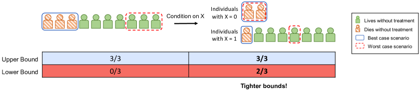
Figure 1: A conceptual figure to build intuition for our main partial identification result (Theorem 4). For simplicity, let the treatment rate $P(T=0)=0.3$ and mortality rate $P(Y(0)=1)=0.3$. We denote upper (blue) /lower (red) bounds on treatment rate among the needy $P(T=1|Y(0)=1,X)$. In the marginal case (left), we see that the bounds are vacuous. However, when we exploit covariate information (right) (e.g., selecting 2 samples from X=0 and 1 sample from X=1), we observe that the bounds are much tighter.

However, in reality, resources are often allocated based on indicators of need or risk that we do not observe (“unobserved confounders”), which could lead us to understate or overstate the amount of inequity. On the one hand, similar rates of allocation across groups could mask inequity, given unobserved differences in need. On the other hand, these differences could explain apparent inequities in allocation across groups.

To make progress in the face of unobserved confounding, we utilize the fact that in many real-world settings, we have data from settings where no individuals received resources (e.g., a time period prior to a new drug entering the market, or a similar region where housing assistance is unavailable). Such data allows us to derive unbiased estimates of what would happen to individuals without the allocation of resources, under an assumption that this baseline risk generalizes to the setting where resources are available. Unfortunately, if unobserved confounders exist, we still cannot identify rates of allocation to needy individuals.

In this setting, we first show that one can derive bounds on the treatment rate among the needy, even without any assumptions on the strength of unobserved confounders. Figure 1 builds intuition for this result, which is given in Assumption 4. We also provide bias-corrected estimators for our bounds that are consistent and asymptotically normal, and extend recent results in the partial identification literature to handle the non-smooth nature of our estimators (Assumption 5). As a result, our bounds can incorporate machine learning (ML) estimators that converge at slower than parametric rates, while retaining the benefit of asymptotic normality (e.g., confidence intervals). Finally, we derive bounds that incorporate assumptions on the plausible strength of unobserved confounding (Definition 3), with corresponding estimators that attain similar asymptotic properties to those discussed above.

We then demonstrate the effectiveness of our framework on real-world data, to audit inequities in the allocation of Paxlovid – a potentially life-saving treatment for COVID-19 patients. Here, we are able to identify racial inequity in the allocation of Paxlovid among COVID-19 outpatients. We observe that even if unobserved confounders had effects on allocation and outcomes similar to that of important observed covariates (Centers for Disease Control and Prevention, 2023), the treatment rate among the needy for Black patients is demonstrably lower than the rate for White and Asian patients.

Finally, we evaluate on semi-synthetic and synthetic tasks using US Census data (Ding et al., 2021), where we know the ground truth counterfactual outcomes. Here, our approach successfully bounds the ground-truth treatment rates among needy individuals, given knowledge of the unobserved confounding strength. Our bounds also contain the actual rates far more often than an ablation that does not incorporate bias correction. In short, our work provides principled conditions under which machine learning estimators can be used as a tool to identify inequity in the allocation of important resources.

2 RELATED WORK

Fairness and Causality The literature on fairness and decision-making is vast, and we will not claim to summarize it here. Of particular relevance to our work is the literature on causal fairness, where fairness metrics are defined with respect to e.g., counterfactual outcomes. Even in this sub-literature, there are a wealth of ways to characterize fairness, such as counterfactual fairness (Kusner et al., 2017) and variants thereof, counterfactual equalized odds (Mishler et al., 2021), and so on. Our choice of metric is similar in spirit to counterfactual equalized odds, and is precisely equivalent to the notion of “opportunity rate” given by Mishler et al. (2021) (see Def. 4.2 of that work).

There are a variety of research directions pursued in the causal fairness literature, such as learning predictive models that lead to fair decisions, or giving conditions under which various notions of causal fairness can be “identified” from data—that is, written in terms of the observed distribution, instead of counterfactual outcomes. Our work is most similar to a nascent line of work considering scenarios where these measures cannot be identified, but can nonetheless be bounded. Closest to our work is that of Rambachan and Coston (2022), who provide bounds on causal fairness measures under a different sensitivity analysis framework. Their framework assumes a bound on the differences in conditional means of potential outcome, whereas our results are derived from bounds on treatment propensities (see Section 4.4). However, the most notable distinction from their work is that we additionally derive bounds that partially identify inequity without any assumptions on the strength of confounders, under our assumption on the availability of pre- and post-treatment periods.

Partial Identification and Sensitivity Analysis In statistics and econometrics, partial identification refers to the derivation of bounds on causal quantities when the exact value cannot be identified from assumptions (Manski, 2003). Sensitivity analysis often refers to the derivation of bounds under assumptions about the “strength” of unobserved confounding. Sensitivity analysis has been pursued under a variety of models, dating back to Cornfield et al. (1959). We will not attempt to summarize the literature here, except to note a few ideas that we draw upon. First, one insight in our analysis is that incorporating covariate information can improve the tightness of our bounds, an insight similarly leveraged in recent work (Yadlowsky et al., 2018; Levis et al., 2023). Second, our sensitivity model can be viewed as a variant of the sensitivity model introduced by Tan (2006), although our causal quantity of interest differs substantially, requiring the derivation of novel bounds. Finally, we draw inspiration from the sensitivity analysis literature to assess the plausibility of our sensitivity parameters via an informal comparison to the strength of observed confounders (Frank, 2000; Hsu and Small, 2013).

3 PRELIMINARIES

Notation

We use upper-case letters to denote random variables (e.g., $X$), and lower-case letters to denote their realizations (e.g., $x$). We use $X\in\mathcal{X}$ to denote covariates, $T\in\{0,1\}$ to denote treatment, and $Y\in\{0,1\}$ to denote a binary outcome. We let $Y=1$ denote an adverse outcome (e.g., mortality), and $Y=0$ denote a benign outcome (e.g., survival). We additionally define the potential outcome $Y(0)$ as the outcome of each individual without treatment.

Given our interest in identifying inequity across different subpopulations, we use $G\in\{1,\ldots,K\}$ to denote subpopulation membership, where group membership is a known function of $X$. We define some quantities (e.g., Definition 1 and some bounds) in terms of the overall population for simplicity of notation, where the extension to group-wise quantities is straightforward.

We further use $D\in\{0,1\}$ to denote whether a sample belongs to pre-treatment or post-treatment data. Pre-treatment data ($D=0$) is drawn from a setting where the resource is not available (e.g., a time period before a drug entered the market) and post-treatment data ($D=1$) from a setting where the resource is available. We consider our data to be drawn from a common distribution $P$, where $P(\cdot\mid D=0)$ and $P(\cdot\mid D=1)$ denote pre- and post-treatment distributions respectively.

Availability of Treatment and Outcome Data

During the pre-treatment period ($D=0$), the treatment is not available by definition, and so $D=0\implies T=0$. In post-treatment data (where $D=1$), we do not assume access to outcome data—for instance, the outcome of interest may be a long-term outcome not immediately measurable in the post-treatment period. As a result, when $D=1$, we set $Y$ to an arbitrary value. Because $T$ is fixed when $D=0$, and because $Y$ is unknown when $D=1$, we observe data as follows

$$(X,T,Y)=\begin{cases}(X,0,Y)&\text{ if $D=0$ (pre-treatment)}\\ (X,T,\sim)&\text{ if $D=1$ (post-treatment)}\end{cases}$$

where $\sim$ indicates that $Y$ is not observed.

4 ANALYSIS OF INEQUITY

4.1 Equity in Treatment Allocation

We first define a notion of effective allocation.

Definition 1 (Treatment Rate Among the Needy).

$$P(T=1\mid Y(0)=1,D=1)$$ (1)

1 captures the proportion of individuals who receive treatment once it is available ($D=1$), among those who would experience an adverse event $Y(0)=1$ if they do not receive treatment. This is similar to the notion of “opportunity rate” in the work of Mishler et al. (2021). Definition 1 suggests a measure of inequity in treatment allocation, when applied to specific subgroups.

Definition 2.

We define inequity in treatment rate among the needy for a pair of subpopulations $g\neq g^{\prime}$ as

$$|P(T=1|Y(0)=1,D=1,G=g)$$

$$\qquad-P(T=1|Y(0)=1,D=1,G=g^{\prime})|$$ (2)

When $Y$ corresponds to mortality, Definition 2 captures the notion that patients who would die if treatment were withheld should receive a potentially life-saving intervention at equal rates across subgroups $G$.

4.2 Identification under Strong Assumptions

We note that it is not possible to directly estimate 1 and 2. In the post-treatment setting, we never observe the outcome $Y$. Further, we can never simultaneously observe $T=1$ and $Y(0)$, which necessitates the use of strong additional assumptions to re-write this quantity in terms of quantities that we do observe. For instance, one could estimate 1 directly if one were willing to assume that $X$ captures all variables that influence both treatment assignment and $Y(0)$, often referred to as the assumption of no unmeasured confounding.

Assumption 1 (No Unmeasured Confounding).

The untreated outcome is independent of treatment in the post-treatment period, given observed covariates, i.e.,

$$Y(0)\perp T\mid X,D=1$$

A main thesis of this work is that Assumption 1 may not be realistic in most real-world settings. Assumption 1 is violated if treatment is allocated on the basis of variables other than $X$, which in turn provide more information on how likely a patient is to experience an adverse outcome without treatment. Given that this assumption may not violated in practice, we will later discuss bounding 1 under a weakened version of Assumption 1 (Section 4.4), and even in the case where we drop Assumption 1 entirely (Section 4.3).

For now, we state assumptions relating the pre- and post-treatment periods, which we maintain throughout.

Assumption 2 (Consistency).

In pre-treatment data, we directly observe the untreated potential outcome, i.e., $D=0\implies Y=Y(0)$.

Assumption 2 is analogous to the assumption of consistency in causal inference and captures the fact that no treatment is available in the pre-treatment period, so all outcomes are untreated outcomes by definition.

Assumption 3 (Covariate Stability).

Within each subgroup, the distribution of covariates of needy patients is the same across pre- and post-treatment periods, i.e.,

$$X\perp D\mid Y(0)=1,G$$

Assumption 3 is a relatively weak assumption, where the observable characteristics $X$ of needy patients (where $Y(0)=1$) are distributed the same across the pre- and post-treatment periods.

Given these assumptions, one can directly identify the treatment rate among the needy from 1.

propositionIdentification Under Assumptions 1, 2 and 3, 1 (conditioned on $G$) can be written as the following functional of the observed distribution $P$

$$P(T=1\mid Y(0)=1,D=1,G=g)$$ (3)

$$\quad=E[P(T=1\mid X,D=1)\mid Y=1,D=0,G=g]$$

This result (with some notational differences) is a known fact in the literature (Coston et al., 2020; Mishler et al., 2021). For completeness, we provide the proof in Section A.2. Notably, as discussed above, this result requires the hard-to-justify assumption that there are no unmeasured confounding variables (Assumption 1). In the following sections, we develop bounds under different relaxations of this assumption.

4.3 Partial Identification under Arbitrary Unmeasured Confounding

To begin, we consider the case where we consider Assumption 1 to be unrealistic and drop it entirely. We demonstrate that it is still possible to obtain informative bounds on the treatment rate in 1 that can be estimated from data, and provide intuition as to why informative bounds are possible to obtain. We proceed under one additional assumption linking the pre- and post-treatment periods.

Assumption 4 (Stable Baseline Risk).

Across the pre- and post-treatment periods, the conditional baseline risk (i.e., the risk of an adverse outcome without treatment) does not change, i.e.,

$$Y(0)\perp D\mid X$$

This is the key assumption relating the pre- and post-treatment periods, which allows us to estimate the baseline risk in the post-treatment period, by leveraging data from pre-treatment period. We expect it to be satisfied when the underlying mechanistic or biological determinants or risk are unchanged around the time period a treatment was introduced. To build further intuition, we depict a causal graph (Figure 2) where Assumptions 3 and 4 hold, but no unmeasured confounding (Assumption 1) fails to hold.

To build intuition for our first main result, consider an extreme case where all individuals will die without treatment. Here, the treatment rate among the needy is simply given by the observed treatment rate. Our result gives informative bounds in less extreme scenarios: For instance, suppose we knew that out of 100 patients, 90 would die if untreated, and that we have treated 50 patients. In this case, the worst-case scenario is that we have treated all 10 patients who would not die if untreated, but we must have treated at least 40 of the patients who would die if untreated.

To begin to formalize this idea, consider the simplified scenario where $Y(0)\perp D$, a stronger version of Assumption 4. Further, observe that $P(T=1,Y(0)=1\mid D=1)\leq P(T=1\mid D=1)$, which yields

$$P(T=1|Y(0)=1,D=1)\leq\frac{P(T=1\mid D=1)}{P(Y(0)=1\mid D=0)}$$

where we switch $D=1$ for $D=0$ in the denominator due to the assumed independence. Note that $P(T=1\mid D=1)$ and $P(Y(0)=1\mid D=0)$ are both observable (in the post- and pre- periods respectively). Unfortunately, this bound may be vacuous on its own (e.g. if $P(Y(0)=1)$ is small). We can sharpen it by noting that the same inequality holds at every value of the covariates $X$, under Assumption 4, such that

$$P(T=1|Y(0)=1,D=1,X)\leq\frac{P(T=1|X,D=1)}{P(Y(0)=1|X,D=0)}.$$

Now, given calibrated classifiers for the treatment and outcome (to estimate the numerator and denominator), the bound will become tighter. Averaging over the appropriate distribution for $X$ then yields a tighter overall bound. To further build intuition, see Figure 1. This idea is formalized in the following theorem.

[Bounds under arbitrary unmeasured confounding]theoremBounds Consider the setting described in Section 3. Under Assumptions 2, 3 and 4, and if there exists a positive constant $\gamma$ such that $P(Y(0)=1\mid D=1,X=x)>\gamma$, then

$$\psi^{l}\leq P(T=1|Y(0)=1,D=1)\leq\psi^{u}$$

where

$$\psi^{l}\coloneqq E[\max\{\theta_{1}^{l}(X),\theta_{2}^{l}(X)\}]$$

$$\psi^{u}\coloneqq E[\min\{\theta_{1}^{u}(X),\theta_{2}^{u}(X)\}]$$

$$\theta_{1}^{l}(X)\coloneqq\frac{P(D=0|X)}{P(Y=1,D=0)}\Big{(}P(T=1|D=1,X)$$

$$\qquad\qquad\qquad+P(Y|D=0,X=x)-1\Big{)}$$

$$\theta_{2}^{l}(X)\coloneqq 0$$

$$\theta_{1}^{u}(X)\coloneqq\frac{P(D=0|X)P(T=1|D=1,X)}{P(Y=1,D=0)}$$

$$\theta_{2}^{u}(X)\coloneqq\frac{P(D=0|X)P(Y=1|D=0,X)}{P(Y=1,D=0)}$$

The proof is given in Appendix A.3. At a high level, we first derive bounds ($\psi^{l},\psi^{u}$) on the quantity of interest. The max/min structure in each bound arises from the complementary fact that the probabilities are upper- and lower-bounded by both a quantity we develop and by 1 and 0 (respectively). The max/min takes the tighter of these two bounds at every level of the covariates. The underlying intuition for our result is that we incorporate information about $X$ in our bound, and estimate these quantities (e.g., $\theta_{1}^{l}(X),\theta_{2}^{l}(X)$) with machine learning (ML) models. With these estimates, we compute the expectation over the conditional distribution over $X$ to produce our bounds $\psi^{l}$ and $\psi^{u}$. This results in a tighter bound, when compared to using population-level bounds, e.g., only looking at the marginals over $T$ and $Y$.

We remark that Theorem 4 expresses our upper and lower bounds only in terms of functions of the observed data, i.e., potential outcomes do not appear in the expression. This establishes that the bounds are identified from the observed data (and without any assumption on the presence of confounders).

Figure 2: A causal graph consistent with Assumptions 3 and 4, even given unobserved (light gray) confounders $C$. Dark gray variables are observed. This causal structure is sufficient, but not necessary, for our assumptions to hold: See Section A.1 for more details.

Estimation of Partial Identification Bounds

Given the identification results in Assumption 4, we are ready to construct estimators of the upper and lower bounds $\psi^{u},\psi^{l}$. We define the following short-hand for the relevant conditional distributions

$$\mu(x) \coloneqq E[Y\mid D=0,X=x]$$ (4)

$$\pi(x) \coloneqq E[T\mid D=1,X=x]$$ (5)

$$g(x) \coloneqq E[D=0\mid X=x]$$ (6)

These conditional expectations can be estimated by training classifiers $\hat{\mu},\hat{\pi}$ on the pre- and post-treatment data respectively, and $\hat{g}$ to distinguish the two. These are referred to as “nuisance functions”, quantities that we have to estimate as part of estimating our bounds, but which are not of intrinsic interest. The simplest strategy would be to “plug-in” such estimators wherever the corresponding conditional expectation appears in the expression for $\psi^{l}$ or $\psi^{u}$. However, it is difficult to provide guarantees for this plug-in estimator, as ML models generally converge slower than $O(n^{-\frac{1}{2}})$, creating substantial bias in our estimate of the bound.

Our proposed method is instead based on influence functions and semiparametric estimation to find and subtract a first-order approximation to the bias of the plug-in estimator. The corresponding estimators will then converge at $O(n^{-\frac{1}{2}})$ rates even if the ML models converge more slowly (as nonparametric methods typically will) and enable us to give valid confidence intervals based on asymptotic normality.

To present our estimator for the upper bound, define $d^{u}(x)\in\arg\min\{\theta_{1}^{u}(x),\theta_{2}^{u}(x)\}$ to be the identity of a bound achieving the minimum value at $x$, with $\hat{d}^{u}(x)$ being the same quantity estimated from the plugin estimate of $\hat{\theta}$. Our proposed estimator is

$$\varphi^{u}(P,d)\coloneqq\theta_{d(X)}^{u}(X)+\lambda^{u}_{d(X)}(X,Y,D,T)$$ (7)

$$\hat{\psi}^{u}(\hat{P})\coloneqq E_{\hat{P}}\left[\varphi(\hat{P},\hat{d}^{u})\right]$$

where we will employ the common strategy of estimating the expectations and the nuisance functions in $\hat{\theta}$ and $\hat{\lambda}$ on independent samples (averaging over $K$-fold cross-validation). We now present the detailed construction and analysis of this estimator, including the bias-correction term $\lambda$ and asymptotic guarantees. Our estimator for the lower bound is defined analogously, using an $\arg\max$.

Bias-corrected estimators

The influence function can be used to provide a first-order approximation to the bias of the estimator; subtracting off this bias will (hopefully) leave a remainder that depends in second order on error of the nuisance functions. Let $\theta_{1}^{u}=E[\theta_{1}^{u}(X)]$ and $\theta_{2}^{u}=E[\theta_{2}^{u}(X)]$. We now derive the influence functions corresponding to $\theta_{1}^{u}$ and $\theta_{2}^{u}$.

lemmaInfluenceUpper The influence functions for $\theta_{1}^{u}$ and $\theta_{2}^{u}$ are given by

$$IF(\theta_{1}^{u})=$$

$$\frac{1}{P(Y=1,D=0)}\Big{(}-\frac{1[Y=1,D=0]}{P(Y=1,D=0)}E_{P}[g(X)\pi(X)]+$$

$$\qquad+g(X)\pi(X)+1[D=1](T-\pi(X))\frac{g(X)}{1-g(X)}+$$

$$\qquad+\pi(X)(1[D=0]-g(X))\Big{)}$$

$$IF(\theta_{2}^{u})=\frac{1[D=0]}{P(Y=1,D=0)}\Big{(}\mu(X)$$

$$\qquad-E[\mu(X)|D=0]\left(\frac{1[Y=1]}{P(Y=1|D=0)}\right)+(Y-\mu(X))\Big{)}.$$

To obtain first-order bias-corrected estimators, we set $\lambda^{u}$ in 7 to the values

$$\lambda_{1}^{u}=IF(\theta_{1}^{u}) \lambda_{2}^{u}=IF(\theta_{2}^{u}).$$ and

Similarly, let $\theta_{1}^{l}=E[\theta_{1}^{l}(X)]$ and $\theta_{2}^{l}=E[\theta_{2}^{l}(X)]$. Then, we can derive their influence functions as follows

lemmaInfluenceLower The influence functions for $\theta_{1}^{l}$ and $\theta_{2}^{l}$ are given by

$$IF(\theta_{1}^{l})=IF(\theta_{1}^{u})+\frac{1}{P(Y=1,D=0)}\Big{(}\frac{-1[Y=1,D=0]}{P(Y=1,D=0)}$$

$$\qquad\qquad\qquad\cdot E_{P}[g(X)(\mu(X)-1)]+1[D=0](Y-1)\Big{)}$$

$$IF(\theta_{2}^{l})=0.$$

To obtain first-order bias-corrected estimators, we set

$$\lambda_{1}^{l}=IF(\theta_{1}^{l}) \lambda_{2}^{l}=0.$$ and

We leave the proofs of the influence functions and bias-corrected estimators of our upper and lower bounds to Appendix A.5 and A.6, respectively.

Asymptotics for nonsmooth bounds

Providing inferential guarantees for our final bounds is complicated by the fact that each is the expectation of a nonsmooth function, i.e., averaging over a max or min operator. As we have derived influence functions for the smooth functions $\theta_{1}^{l}$ and $\theta_{2}^{l}$, simple asymptotic normality results (albeit for weaker bounds) can be obtained by dropping the min and max, averaging only over one or the other separately. These can be obtained via standard techniques, and are given in Appendix A.4.

For the stronger nonsmooth bounds, we will need an additional assumption to guarantee asymptotic normality and provide valid confidence intervals. Our results build on a framework introduced by Levis et al. (2023) in the context of estimating bounds in instrumental variable models. They show that bounds with a similar expectation-of-max of structure can be estimated under a margin condition which requires that the terms appearing in the max (or min) are separated with sufficiently high probability. We generalize their framework beyond the instrumental variable setting to provide conditions for estimation of any expectation-of-max structure where the terms inside the max admit first-order bias-corrected estimators. Suppose we want to estimate a bound of the form $E[\max_{j=1...J}\theta_{j}(X)]$ (in general, we can allow more than two components, although this is all we use so far). We adopt a margin assumption similar to Levis et al. (2023), itself inspired by similar assumptions used in a variety of other statistical settings (Audibert and Tsybakov, 2007; Luedtke and Van Der Laan, 2016; Kennedy et al., 2020).

Assumption 5.

For some fixed $\alpha>0$, $P\left[\min_{j\neq d(X)}\theta_{d(X)}(X)-\theta_{j}(d(X))\leq t\right]\lesssim t^{\alpha}$

This condition will be satisfied when the distribution of $\theta_{d(X)}(X)-\theta_{j}(d(X))$ has bounded density near 0. With this condition, we obtain the following result for the stronger estimator of the upper bound. [Asymptotic Normality of Estimators]theoremNormality Let $\hat{\theta}$ denote the plugin estimate of any of the individual components of each bound. Under the conditions that Assumption 5 is satisfied, $\mu$ and $g$ are lower bounded, and each $\hat{\theta}$ is consistent (i.e., $||\hat{\theta}-\theta||=o_{P}(1)$), the error of the estimator satisfies.

$$\hat{\psi}^{u}-\psi^{u}=O_{P} \Big{(}||\hat{\theta}^{u}_{j}-\theta^{u}_{j}||_{\infty}^{1+\alpha}$$

$$+\max_{j=1,\ldots,J}E_{P}[\hat{\theta}^{u}_{j}+\hat{\lambda}^{u}_{j}-\theta^{u}_{j}]\Big{)}+O_{P}(n^{-\frac{1}{2}})$$

Provided that $\hat{\pi}$ and $\hat{g}$ converge at a $o_{P}(n^{-\frac{1}{4}})$ rate, and the plugin estimators satisfy $||\hat{\theta}^{u}_{j}-\theta^{u}_{j}||_{\infty}^{1+\alpha}=o_{P}(n^{-\frac{1}{2}})$, then $\hat{\psi}_{u}$ is asymptotically normal with

$$\sqrt{n}(\hat{\psi}^{u}-\psi^{u})\to N(0,Var(\varphi(P,d))).$$

The full proof is contained in Appendix B. The error in our bias-corrected estimator of $\theta_{1}^{u}$ reduces to a sum of (i) a term on the order of $P(Y=1,D=0)-\hat{P}(Y=1,D=0)$, which converges at a parametric rate and (ii) a product of differences in $(\hat{\pi}-\pi)$ and $(\hat{g}-\hat{g})$. As such, we only require each of these estimators to converge at the slower rate of $o_{P}(n^{-\frac{1}{4}})$ to achieve our fast rate. The plugin estimators $\hat{\theta}$ may also converge at slower rates depending on $\alpha$ in the margin condition, e.g., if $\alpha\geq 1$ then $o_{P}(n^{-\frac{1}{4}})$ suffices for them as well.

As asymptotic normality holds, we can construct standard confidence intervals for the relevant estimator $\hat{\psi}$. First, we can obtain a consistent estimator of the variance of $\hat{\psi}$ as

$$\hat{\sigma}^{2} =\frac{1}{n}\sum_{i=1}^{n}\left(\hat{\psi}(X_{i})-\frac{1}{n}\sum_{j=1}^{n}\hat{\psi}(X_{j})\right)^{2},$$

which results in a confidence interval

$$\widehat{CI}_{\psi^{l},\psi^{u}}=\left[\hat{\psi^{l}}-z_{1-\alpha/2}\frac{\hat{\sigma}^{l}}{\sqrt{n}},\hat{\psi^{u}}+z_{1-\alpha/2}\frac{\hat{\sigma}^{u}}{\sqrt{n}}\right],$$

where $\hat{\sigma}^{l}$ and $\hat{\sigma}^{u}$ are the estimated standard deviations of $\psi^{l}$ and $\psi^{u}$. Therefore, we can use our estimators, and their corresponding confidence intervals to provide confidence bounds on the treatment allocation rates of interest. When these intervals are disjoint and non-overlapping across groups, our results suggest the presence of inequity (i.e., when our assumptions hold).

4.4 Sensitivity Analysis under Bounded Confounding

If it is plausible to impose an assumption that confounding in treatment assignment is bounded, we can in turn obtain tighter bounds on our estimand of interest. We introduce a sensitivity parameter $\gamma$ that captures the extent of the impact of the potential outcome $Y(0)$ on treatment assignment, similar in spirit to the sensitivity model used by Tan (2006), adapted to our problem setting. This model allows us to, under the assumption that confounding is limited, assess whether there are verifiable discrepancies in allocation rates across subgroups. With this framework, we can vary $\gamma$ over a range of values to determine to how much confounding our finding is robust.

Definition 3.

We define a sensitivity parameter $\gamma$ as

$$\frac{1}{\gamma}\leq\frac{P(T=1|Y(0)=0,D=1,X)}{P(T=1|Y(0)=1,D=1,X)}\leq\gamma.$$

We note that $\gamma=\infty$ is equivalent to arbitrary unmeasured confounding. In this scenario, we can recover the result in Theorem 4. Assuming a finite value of $\gamma$, we obtain the following stronger upper and lower bounds: [Bounds with $\gamma$]theoremIdentificationGamma Using Definition 3, we achieve the following set of bounds

$$\psi^{l,\gamma}\leq P(T=1|Y(0)=1,D=1,X)\leq\psi^{u,\gamma}$$

where

$$\psi^{l,\gamma}\coloneqq E[\max\{\theta_{1}^{l,\gamma},\theta_{2}^{l,\gamma}\}]$$

$$\psi^{u,\gamma}\coloneqq E[\min\{\theta_{1}^{u,\gamma},\theta_{2}^{u,\gamma}\}]$$

$$\theta_{1}^{l,\gamma}\coloneqq\theta_{1}^{l}$$

$$\theta_{2}^{l,\gamma}\coloneqq\frac{\scriptstyle P(T=1|D=1,X)}{\scriptstyle P(Y(0)=1|D=1,X)+\gamma(1-P(Y(0)=1|D=1,X))}$$

$$\theta_{1}^{u,\gamma}\coloneqq\frac{\scriptstyle P(T=1|D=1,X)}{\scriptstyle P(Y(0)=1|D=1,X)+\frac{1}{\gamma}(1-P(Y(0)=1|D=1,X))}$$

$$\theta_{2}^{u,\gamma}\coloneqq\theta_{2}^{u}$$

We defer the proof to Appendix A.8. This is again similar in style to Theorem 4, where we incorporate covariate information to achieve tigther bounds $\psi^{l,\gamma}$ and $\psi^{u,\gamma}$. We note that these bounds converge to our earlier ones as $\gamma\to\infty$, and at $\gamma=1$ (i.e., no confounding with respect to $Y(0)$), which implies point identification at $P(T=1|Y(0)=1,D=1,X)=P(T=1|D=1,X)$. Notably, the lower bound takes a max over a new quantity (that is dependent on $\gamma$) as well as the two terms appearing in the bound in Assumption 4 (valid without any assumption on confounding).

We present a high-level overview of methods and results for the construction of estimators for the bounds in Definition 3, with details in Appendix A.9. The picture is very similar to before: we can construct first order bias-corrected estimators for each term appearing inside the max and min, by adding the expectation (over $\hat{P})$ of the influence functions we have derived. One option, requiring fewer assumptions, is to take expectations over each term individually and then choose the stronger of the bounds after averaging (applying a multiple-comparisons correction such as union bound to the level of the CIs). Under Assumption 5, we further obtain that the expectation-of-max estimator is also asymptotically normal with sufficiently fast convergence rates for the estimators of the nuisance functions, which we defer to Appendix B.

4.5 Benchmarking Sensitivity Analysis

The sensitivity parameter $\gamma$ is an assumption, not something we can estimate from data. To assess the plausibility of different $\gamma$ values, we can compute an analogous $\gamma^{\prime}$ for an observed random variable (e.g., diabetes) which is held out of the covariate set $X$. This quantity can be estimated from data to perform benchmarking.

Similarly, we determine this value of $\gamma^{\prime}$ by training a discriminative model to compute the following inequality, where $X^{\prime}$ denotes all covariates $X$ except $Z$,

$$\frac{1}{\gamma^{\prime}}\leq\frac{P(T=1|Z=0,D=1,X^{\prime})}{P(T=1|Z=1,D=1,X^{\prime})}\leq\gamma^{\prime},$$

where $Z$ is the random variable that represents if the patient has the covariate of interest and where $Z\notin X^{\prime}$.

5 RESULTS

We apply our analysis framework to understand treatment allocation inequity in the real-world setting of Paxlovid allocation for high-risk COVID-19 outpatients, as well as semi-synthetic and synthetic settings, to demonstrate that our approach indeed successfully captures the ground-truth rates for treatment among the needy, when controlling for the true amount of unobserved confounding. In our experiments, we use a logistic regression model for our estimators. For each estimator, we perform cross-fitting/sample-splitting over 5 disjoint folds. In all of our reported bounds, we use a 95% confidence interval; in the case where our bounds use two quantities, we use a 97.5% confidence interval for each, so that the resulting confidence interval is 95% (via an application of the union bound).

5.1 Dataset and Cohort Definition

We use the NCATS NC3 cohort (Haendel et al., 2020), consisting of national line-level data of $18,438,581$ total patients, including $7,149,421$ confirmed COVID-19 positive patients, pooled from $76$ different data sharing centers across the United States. We focus our analysis on outpatients with a positive SARS-CoV-2 test result, satisfying eligibility requirements (see Appendix C).

5.2 Real-world Study Results

Figure 3: Upper (solid) and lower (dashed) bounds for $P(T=1|Y(0)=1,D=1,G=g)$ are computed for each racial group $g$, with varying values of $\gamma\in[1,1.05]$. The shaded area represents a 95% confidence interval.

Under bounded unobserved confounding as in Definition 3, with parameter $\gamma$, we are able to identify non-overlapping bounds for our quantity of interest $P(T=1|Y(0)=1,D=1)$ for particular subgroups. We identify non-overlapping bounds between Black and White patients ($\gamma\leq 1.12$) as well as Black and Asian patients ($\gamma\leq 1.2$). Hence, treatment rates for Black patients that would die without treatment are strictly lower than treatment rates for White and Asian patients, up to $\gamma=1.12$, $\gamma=1.2$ respectively, highlighting substantial inequity. For a better interpretation of $\gamma$, we perform the following benchmarking analysis.

5.3 Benchmarking Sensitivity Analysis

In our benchmarking, we select diabetes as our covariate of interest, based on its well-documented association with high risk of severe COVID-19 (Centers for Disease Control and Prevention, 2023). We again proceed by training a classifier to predict treatment, letting $Z$ be diabetes and $X^{\prime}$ be all other covariates. Then, we compute the following ratio on post-treatment test data, using counterfactual features of having diabetes ($Z=1$) or not having diabetes ($Z=0$) for each patient:

$$\frac{1}{\gamma^{\prime}}\leq\frac{P(T=1|Z=0,D=1,X^{\prime})}{P(T=1|Z=1,D=1,X^{\prime})}\leq\gamma^{\prime}.$$

We observe that the smallest value of $\gamma^{\prime}$ that satisfies the above equation for all post-treatment test data is $1.09$. Therefore, our result in identifying disparities in allocation (for example, non-overlapping bounds for (1) Black and White $\gamma\approx 1.12$ and (2) Black and Asian $\gamma\approx 1.2$ ) is robust to an unobserved confounding variable that exhibits an influence on COVID-19 treatment allocation up to the impact of a patient’s diabetes, which is evidenced to be associated with high risk of severe COVID-19 (Centers for Disease Control and Prevention, 2023).

5.4 Semi-synthetic and Synthetic Settings

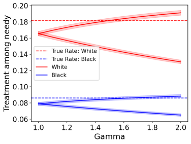
Figure 4: (Semi-Synthetic Data) Upper and lower bounds for treatment rate among the needy, with 95% confidence intervals, for each racial group $g$, with varying values of $\gamma\in[1,2]$ (true value of $\gamma=1.5$).

We generate a semi-synthetic task from the Folktables dataset comprised of US Census data (Ding et al., 2021). In these tasks, we know the ground truth rates of treatment among the needy, so we can study whether our bounds are indeed valid and compare them to other naive approaches. Here, we use two racial groups of White and Black patients, and we simulate both $Y$ and $T$. We define $Y=T*Y(1)+(1-T)*Y(0)$ and sample $Y(0)\sim\text{Bernoulli}(\sigma(|x|_{1}+2))$ and $Y(1)\sim\text{Bernoulli}(\sigma(|x|_{1}+2)/2)$, where $\sigma$ represents the sigmoid function. To produce a known value of $\gamma,$ we use $Y(0)$ to confound the generation of $T$. We sample $T\sim\text{Bernoulli}(p)$. For White patients, $p=\sigma(|x|_{1}-1)$ and for Black patients, $p=\sigma(|x|_{1}-2)$. If $Y(0)=1$, we divide $p$ by 1.5, making $\gamma=1.5$.

We generate our fully synthetic task in a similar fashion, where our covariates are sampled from a 2D Gaussian of $\mathcal{N}(0,0.2)\times\mathcal{N}(0,0.1)$. In this task, we control $\gamma=1.5$, similar to the semi-synthetic task.

In our semi-synthetic experiments, we observe that our estimates of our bounds successfully capture the true treatment rates among the needy, given the true amount of unobserved confounding (i.e., $\gamma=1.5$) (Figure 4). To the best of our knowledge, no other approach provides valid bounds in this setting. To illustrate the benefit of our approach over simpler plugin estimates, we run synthetic experiments (Figure 5) over 100 different trials given limited data (4000 $\sim$ 20000 samples). We capture the rates at which our bounds and the naive plugins capture the true rates given the actual value of $\gamma=1.5$. We observe that our bounds capture the true rates at a significantly higher rate given limited data compared to naive plug-in based approaches.

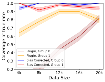
Figure 5: (Synthetic Data) Accuracy of our bias-corrected bounds compared to their naive plugin counterparts in capturing the true treatment rates. We use the derived 95% confidence interval from our bias-corrected estimates for both methods.

6 DISCUSSION

In this work, we introduce a principled approach that uses machine learning to audit need-based inequity under unobserved confounding. We introduce a causal notion of equity whereby allocation rates should be equalized across groups when conditioning on the population who would suffer an adverse outcome without resource allocation. We demonstrate that our approach can robustly quantify need-based inequity, even in the presence of unobserved confounding factors. We provide bias-corrected estimators for our bounds that satisfy desirable statistical properties, even when the underlying ML models converge at slow rates. Furthermore, we apply our method to analyze a real-world case study of Paxlovid allocation to high-risk COVID-19 outpatients, motivated by several recent studies that have demonstrated racial disparities in treatment allocation (Sullivan et al., 2022; Tarabichi et al., 2023; Wiltz et al., 2022; Kuehn, 2022), and we find that observed inequity between racial groups cannot be explained by unobserved confounders at the same influence of important observable covariates. More broadly, we remark that our setting and design are quite general and have wide potential applications; they can easily be applied to different applications such as the creation of new services, government programs, and so on. Equivalently, it can be applied to policies, benefits, or treatments that roll out in one location and not the other.

Acknowledgements

We would like to thank Angel Desai for the helpful discussion during the early phase of this project. We would also like to thank the anonymous reviewers for their valuable feedback. YB was supported in part by the AI2050 program at Schmidt Sciences (Grant G-22-64474) and also gratefully acknowledges the NSF (IIS2211955), UPMC, Highmark Health, Abridge, Ford Research, Mozilla, the PwC Center, Amazon AI, JP Morgan Chase, the Block Center, the Center for Machine Learning and Health, and the CMU Software Engineering Institute (SEI) via Department of Defense contract FA8702-15-D-0002, for their generous support of ACMI Lab’s research. DS was supported by the Bosch Center for Artificial Intelligence, the ARCS Foundation, and the National Science Foundation Graduate Research Fellowship under Grant No. DGE2140739.

The analyses described in this publication were conducted with data or tools accessed through the NCATS N3C Data Enclave https://covid.cd2h.org and N3C Attribution & Publication Policy v 1.2-2020-08-25b supported by NCATS U24 TR002306, Axle Informatics Subcontract: NCATS-P00438-B. This research was possible because of the patients whose information is included within the data and the organizations (https://ncats.nih.gov/n3c/resources/data-contribution/data-transfer-agreement-signatories) and scientists who have contributed to the on-going development of this community resource [https://doi.org/10.1093/jamia/ocaa196].

Appendix A Additional Proofs & Statements

In this section, we provide additional remarks as well as the omitted proofs for the Propositions, Lemmas, and Theorems in the main paper, except for Assumption 5. The proof of Assumption 5 is separately located in Appendix B.

A.1 Representing Assumptions in a Causal Graph

In Figure 2 we gave an illustrative causal graph, and claimed that this causal structure is sufficient, but not necessary, for our assumptions to hold. A more precise characterization is given here, using the framework of single-world intervention graphs (SWIGs), developed by Richardson and Robins (2013). Single-world intervention graphs are a useful tool for relating assumptions that use potential outcome notation to those which use the framework of causal directed acyclic graphs.

Figure 6: Example of a single-world intervention graph (SWIG) (Richardson and Robins, 2013), mirroring Figure 2, that satisfies Assumptions 3 and 4, but where unobserved confounding is present. Note that we use $Y_{0}$ in lieu of $Y(0)$ for consistency with typical SWIG notation, but these notations are equivalently representing the potential outcome under $T=0$. We use node-splitting notation, where all outgoing edges from $T$ propagate the chosen value $T=0$, all incoming edges go to $T$, and there is no connection between $T$ and $T=0$. This graph illustrates causal relationships in the ‘single world’ where we intervene upon $T$ and set it to the chosen value.

Figure 6 applies the intervention $T=0$ to the causal graph given in Figure 2, via a ‘node splitting’ operation (see Richardson and Robins (2013) for more details), where the node $T$ is split, all incoming edges go to $T$, and all outgoing edges propagate the value $T=0$, yielding $Y_{0}$ instead of $Y$ in this example. This graph allows us to characterize the causal relationships between the potential outcome $Y_{0}$ and other variables, in the ‘single world’ where we intervene upon $T$ and set it to the desired value $T=0$. Note that in the resulting graph, the nodes $T$ and $T=0$ are not connected. From d-separation in the graph given in Figure 6, we can observe that both Assumption 3 and Assumption 4 hold, namely that

$$X \perp D\mid Y_{0} Y_{0} \perp D\mid X,$$ and

where the former implies Assumption 3 and the latter is equivalent to Assumption 4. However, our assumptions are only a subset of the implications of this causal structure. For instance, this causal structure would imply similar relationships for $Y_{1}$, which does not appear in our assumptions. Hence our claim that this causal structure is sufficient, but not necessary, for our assumptions to hold.

A.2 Proof of Assumption 3

*

Proof.

$$P(T=1\mid Y(0)=1,D=1,G=g)$$

$$\quad=\int_{x}P(T=1\mid X=x,Y(0)=1,D=1,G=g)$$

$$\qquad\qquad\cdot P(X=x\mid Y(0)=1,D=1,G=g)dx$$

$$\quad=\int_{x}P(T=1\mid X=x,D=1)$$

$$\qquad\qquad\cdot P(X=x\mid Y=1,D=0,G=g)dx$$

where the first equality follows from standard rules of probability, and the second equality invokes our three assumptions given above. ∎

A.3 Proof of Theorem 4

*

Proof.

First, we remark that

$$P(T=1|D=1,X)=P(Y(0)=1|D=1,X)P(T=1|Y(0)=1,D=1,X)$$

$$\qquad+P(Y(0)=0|D=1,X)P(T=1|Y(0)=0,D=1,X)$$

We can rearrange this equation, giving us that

$$P(T= 1|Y(0)=1,D=1,X)=$$

$$\frac{P(T=1|D=1,X)-P(Y(0)=0|D=1,X)P(T=1|Y(0)=0,D=1,X)}{P(Y(0)=1|D=1,X)}$$

Then, we observe that $0\leq P(T=1|Y(0)=0,D=1,X)\leq 1$, which gives us that

$$P(T=1|Y(0)=1,D=1,X) \leq\frac{P(T=1|D=1,X)}{P(Y(0)=1|D=1,X)},$$

$$P(T=1|Y(0)=1,D=1,X) \geq\frac{P(T=1|D=1,X)-P(Y(0)=0|D=1,X)}{P(Y(0)=1|D=1,X)}.$$

Next, we remark that our quantity of interest is given by

$$P(T=1|Y(0)=1,D=1)=E_{X}[P(T=1|Y(0)=1,D=1,X)|Y(0)=1,D=0],$$

where we can switch from $D=1$ to $D=0$ in our conditional expectation due to Assumption 3. Then, we note that in our estimate of $P(T=1|Y(0)=1,D=1,X)$, we can apply simple $[0,1]$ bounds since it is a probability. Therefore, we get that our target is now given by

$$E\left[\max\left\{0,\frac{P(T=1|D=1,X)-P(Y(0)=0|D=1,X)}{P(Y(0)=1|D=1,X)}\right\}\mid Y=1,D=0\right]$$

$$\qquad\leq P(T=1|Y(0)=1,D=1)\leq E\left[\min\left\{1,\frac{P(T=1|D=1,X)}{P(Y(0)=1|D=1,X)}\right\}\mid Y=1,D=0\right]$$

Finally, we can convert this to be computed over the unconditional expectation as follows. The upper bound is given by a min over two terms. The term involving 1 simplifies to

$$E[1|Y=1,D=0] =\int_{x}1\cdot P(x|Y=1,D=0)$$

$$=\int_{x}P(Y=1,D=0|x)\frac{P(x)}{P(Y=1,D=0)}$$

$$=\frac{1}{P(Y=1,D=0)}E\left[P(Y=1,D=0|X)\right]$$

$$=\frac{1}{P(Y=1,D=0)}E\left[P(Y=1|D=0,X)\cdot P(D=0|X)\right]$$

The other term is given by

$$E\left[\frac{P(T=1|D=1,X)}{P(Y(0)=1|D=1,X)}\mid Y=1,D=0)\right]$$

Note that with Assumption 4, we can replace the denominator with $P(Y(0)=1|D=0,X)$ as $Y(0)$ and $D$ are independent conditioning on covariates $X$. Then, we have that

$$E\left[\frac{P(T=1|D=1,X)}{P(Y(0)=1|D=1,X)}\mid Y=1,D=0\right] =E\left[\frac{P(T=1|D=1,X)}{P(Y(0)=1|D=0,X)}\mid Y=1,D=0\right]$$

$$=\int_{x}\frac{P(T=1|D=1,X)}{P(Y(0)=1|D=0,X)}P(Y=1,D=0|x)\frac{P(x)}{P(Y=1,D=0)}$$

$$=\frac{1}{P(Y=1,D=0)}E\left[\frac{P(T=1|D=1,X)}{P(Y(0)=1|D=0,X)}P(Y=1,D=0|X)\right]$$

$$=\frac{1}{P(Y=1,D=0)}E\left[P(D=0|X)P(T=1|D=1,X)\right]$$

Next, we can consider the lower bound. The lower bound is given by a max of two terms. The zero term is trivially 0. The other term is given by

$$E\left[\frac{P(T=1|D=1,X)-P(Y(0)=0|D=1,X)}{P(Y=1|D=0)}\mid Y=1,D=0\right]$$

We can again switch $D=1$ to $D=0$ in both the $Y(0)$ term in the numerator and in the term in the denominator using Assumption 4. Then, we get that

$$E\left[\frac{P(T=1|D=1,X)-P(Y(0)=0|D=0,X)}{P(Y=1|D=0)}\mid Y=1,D=0\right] =\int_{x}\frac{P(T=1|D=1,X)-P(Y(0)=0|D=0,X)}{P(Y=1|D=0)}$$

$$\qquad\cdot P(Y=1,D=0|x)\frac{P(x)}{P(Y=1,D=0)}$$

$$=\frac{1}{P(Y=1,D=0)}E\Big{[}P(D=0|X)$$

$$\qquad\frac{P(T=1|D=1,X)-P(Y(0)=0|D=0,X)}{P(Y=1|D=0,X)}\Big{]}$$

$$=\frac{1}{P(Y=1,D=0)}E\Big{[}P(D=0|X)$$

$$\qquad\frac{P(T=1|D=1,X)+P(Y(0)=1|D=0,X)-1}{P(Y=1|D=0,X)}\Big{]}$$

∎

as desired.

A.4 Analysis of Plugin Estimators

We now present some analysis of a standard plugin estimator, which will be useful in proofs in error analysis of our corrected estimators. At a high level, this section demonstrates that a simple plugin estimator for the (ratio) estimand of $E\left[\frac{\pi(X)}{\mu(X)}\right]$ achieves a rate that is a combination of the rates of our estimators of $\pi$ and $\mu$, plus an additional term that is the variance of our plugin estimator.

First, we will prove a technical lemma that bounds the expected error of a ratio estimator that directly takes a ratio of plugins.

Lemma 1.

Let $R=\frac{\pi}{\mu}$, and $\hat{R}=\frac{\hat{\pi}}{\hat{\mu}}$. Then, we have that

$$|E_{x\sim P}[R]-E_{x\sim P}[\hat{R}]|\leq\frac{2}{\delta^{2}}\left(E_{x\sim P}[|\pi-\hat{\pi}|]+E_{x\sim P}[|\hat{\mu}-\mu|]\right),$$

for some $0\leq\delta\leq\mu,\hat{\mu}$.

Proof.

We first observe that

$$|E_{x\sim P}[R]-E_{x\sim P}[\hat{R}]| \leq E_{x\sim P}\left[|R-\hat{R}|\right]$$

$$=E_{x\sim P}\left[|\frac{\pi\hat{\mu}-\hat{\pi}\mu}{\mu\hat{\mu}}|\right]$$

$$\leq\frac{1}{\delta^{2}}E_{x\sim P}\left[|\pi\hat{\mu}-\hat{\pi}\mu|\right]$$

Let $x$ be an arbitrary data point. We observe that

$$\min\{\pi\mu-\hat{\pi}\hat{\mu},\hat{\pi}\hat{\mu}-\pi\mu\}+\pi\hat{\mu}-\hat{\pi}\mu\leq\pi\hat{\mu}-\hat{\pi}\mu\leq+\max\{\pi\mu-\hat{\pi}\hat{\mu},\hat{\pi}\hat{\mu}-\pi\mu\}+\pi\hat{\mu}-\hat{\pi}\mu,$$

since one of $\pi\mu-\hat{\pi}\hat{\mu},\hat{\pi}\hat{\mu}-\pi\mu$ must be non-positive, and one must be non-negative.

We first consider the term of $\pi\mu-\hat{\pi}\hat{\mu}$. This satisfies that

$$\pi\mu-\hat{\pi}\hat{\mu}+\pi\hat{\mu}-\hat{\pi}\mu =\mu(\pi-\hat{\pi})+\hat{\mu}(\pi-\hat{\pi})=(\mu+\hat{\mu})(\pi-\hat{\pi})$$

Then, noting that $\mu,\hat{\mu}\in[0,1]$, we have that

$$|\pi\mu-\hat{\pi}\hat{\mu}+\pi\hat{\mu}-\hat{\pi}\mu|\leq 2|\pi-\hat{\pi}|$$

Next, we can consider the other case of the term $\hat{\pi}\hat{\mu}-\pi\mu$. We have that

$$\hat{\pi}\hat{\mu}-\pi\mu+\pi\hat{\mu}-\hat{\pi}\mu =(\hat{\mu}-\mu)(\pi+\hat{\pi}),$$

and with $\pi,\hat{\pi}\in[0,1]$, we get that

$$|\hat{\pi}\hat{\mu}-\pi\mu+\pi\hat{\mu}-\hat{\pi}\mu|\leq 2|\pi+\hat{\pi}|,$$

Therefore, we observe that

$$|\pi\hat{\mu}-\hat{\pi}\mu| \leq 2\max\{|\hat{\mu}-\mu|,|\pi-\hat{\pi}|\}$$

$$E_{x\sim P}\left[|\pi\hat{\mu}-\hat{\pi}\mu|\right] \leq 2E_{x\sim P}\left[\max\{|\hat{\mu}-\mu|,|\pi-\hat{\pi}|\}\right]$$

$$\leq 2\left(E_{x\sim P}[|\pi-\hat{\pi}|]+E_{x\sim P}[|\hat{\mu}-\mu|]\right)$$

Plugging us in gives us the result that

$$|E_{x\sim P}[R]-E_{x\sim P}[\hat{R}]|\leq\frac{2}{\delta^{2}}\left(E_{x\sim P}[|\pi-\hat{\pi}|]+E_{x\sim P}[|\hat{\mu}-\mu|]\right)$$

∎

Now, we can consider the estimator $E_{\hat{P}}[\frac{T}{\hat{\mu}(X)}]$. To verify consistency, note that as $\hat{P}\to P$ and $\hat{\mu}\to\mu$ we have

$$E_{\hat{P}}\left[\frac{T}{\hat{\mu}(X)}\right]\to E_{P}\left[\frac{T}{\mu(X)}\right]$$

and using iterated expectation yields that

$$E_{T,X\sim P}\left[\frac{T}{\mu(X)}\right]=E_{X\sim P}\left[\frac{E[T|X]}{\mu(X)}\right]=E_{X\sim P}\left[\frac{\pi(X)}{\mu(X)}\right].$$

Next, we analyze the total expected error of this estimator. To start with, note that

$$E_{\hat{P}}\left[\frac{T}{\hat{\mu}(X)}\right]-E_{X\sim P}\left[\frac{\pi(X)}{\mu(X)}\right]=\left(E_{\hat{P}}\left[\frac{T}{\hat{\mu}(X)}\right]-E_{P}\left[\frac{T}{\hat{\mu}(X)}\right]\right)+\left(E_{P}\left[\frac{T}{\hat{\mu}(X)}\right]-E_{P}\left[\frac{\pi(X)}{\mu(X)}\right]\right).$$

Provided that we employ sample splitting, so that $\hat{\mu}$ is trained on an independent sample from the samples used to estimate the expectation $\hat{P}$, the first term is easily controlled in terms of the variance of $\frac{T}{\mu(X)}$. Specifically, suppose that $\hat{P}$ is estimated using $n$ samples. We have that

$$E\left[\left\lvert E_{\hat{P}}\left[\frac{T}{\hat{\mu}(X)}\right]-E_{P}\left[\frac{T}{\hat{\mu}(X)}\right]\right\rvert\right] =E\left[\left\lvert E_{\hat{P}}\left[\frac{T}{\hat{\mu}(X)}\right]-E\left[E_{\hat{P}}\left[\frac{T}{\hat{\mu}(X)}\right]\right\rvert\right]\right]$$

$$\leq\sqrt{\text{Var}\left[E_{\hat{P}}\left[\frac{T}{\hat{\mu}(X)}\right]\right]}=\sqrt{\frac{\text{Var}\left[\frac{T}{\hat{\mu}(X)}\right]}{n}}$$

where the first equality follows because $E_{\hat{P}}\left[\frac{T}{\hat{\mu}(X)}\right]$ is an unbiased estimator for $E_{P}\left[\frac{T}{\hat{\mu}(X)}\right]$, the second line follows by Cauchy-Schwartz, and the third because the samples in $\hat{P}$ are independent.

For the second term, note that since $E_{T,X\sim P}\left[\frac{T}{\mu(X)}\right]=E_{X\sim P}\left[\frac{E[T|X]}{\mu(X)}\right]$, we can apply Lemma 1 with $\hat{\pi}=\pi$ to obtain that

$$\left\lvert E_{P}\left[\frac{T}{\hat{\mu}(X)}\right]-E_{P}\left[\frac{\pi(X)}{\mu(X)}\right]\right\rvert\leq\frac{2}{\gamma^{2}}E_{P}[|\mu(X)-\hat{\mu}(X)|].$$

Combining the bounds on the first and second terms using the triangle inequality yields

$$E\left[\left\lvert E_{\hat{P}}\left[\frac{T}{\hat{\mu}(X)}\right]-E_{X\sim P}\left[\frac{\pi(X)}{\mu(X)}\right]\right\rvert\right]\leq\sqrt{\frac{\text{Var}\left[\frac{T}{\hat{\mu}(X)}\right]}{n}}+\frac{2}{\gamma^{2}}E_{P}[|\mu(X)-\hat{\mu}(X)|].$$

Note that a high-probability bound could be obtained by using a Bernstein bound for the first term combined with any high-probability generalization guarantee for the ML model in the second term.

An analogous argument for the alternate plugin estimator $E_{\hat{P}}\left[\frac{\hat{\pi}(X)}{\hat{\mu}(X)}\right]$ yields the bound on its expected error

$$E\left[\left\lvert E_{\hat{P}}\left[\frac{\pi(X)}{\hat{\mu}(X)}\right]-E_{X\sim P}\left[\frac{\pi(X)}{\mu(X)}\right]\right\rvert\right]\leq\sqrt{\frac{\text{Var}\left[\frac{\hat{\pi}(X)}{\hat{\mu}(X)}\right]}{n}}+\frac{2}{\gamma^{2}}\left(E_{P}[|\mu(X)-\hat{\mu}(X)|]+E_{P}[|\pi(X)-\hat{\pi}(X)|]\right).$$

Comparing these two bounds, we observe a form of bias-variance tradeoff. In the second bound, we accumulate additional potential error from the estimation of $\hat{\pi}$ instead of directly plugging in the samples $T$. However, we often expect that $\hat{\pi}$ will have lower variance than $T$ since estimated treatment probabilities will take less extreme values than binary treatment indicators, in which case the variance term will be smaller for the second estimator.

A.5 Proof of Lemma 4.3

Next, we will derive the influence functions for our upper bounds under no additional assumptions. Recall that our estimands are given by

$$\theta_{1}^{u}(X)\coloneqq\frac{P(D=0|X)P(T=1|D=1,X)}{P(Y=1,D=0)}, \theta_{2}^{u}(X)\coloneqq\frac{P(D=0|X)P(Y=1|D=0,X)}{P(Y=1,D=0)}$$

Our relevant conditional distributions (i.e., our nuisance functions) are given by

$$\mu(X)\coloneqq E[Y=1|D=0,X=x],\qquad\pi(X)\coloneqq E[T=1|D=1,X=x],\qquad g(x)\coloneqq E[D=0|X=x]$$

We now proceed to derive the influence functions for our upper bound under no additional assumptions.

*

Proof.

First, we will derive the influence function for $\theta^{u}_{1}$.

$$IF\left(\theta^{u}_{1}\right)= IF\left(\frac{1}{P(Y=1,D=0)}\right)E_{P}[g(X)\pi(X)]+\frac{1}{P(Y=1,D=0)}IF\left(E_{P}[g(X)\pi(X)]\right)$$

$$=- \frac{1[Y=1,D=0]-P(Y=1,D=0)}{P(Y=1,D=0)^{2}}E_{P}[g(X)\pi(X)]$$

$$+\frac{1}{P(Y=1,D=0)}\sum_{x}(1[X=x]-p(x))(g(x)\pi(x))$$

$$+\frac{1}{P(Y=1,D=0)}\sum_{x}p(x)\left(\frac{1[X=x]}{P(X=x)}(1[D=0]-g(x))\right)\pi(x)$$

$$+\frac{1}{P(Y=1,D=0)}\sum_{x}p(x)g(x)\left(\frac{1[D=1,X=x]}{P(D=1,X)}(T-\pi(x))\right)$$

$$=- \frac{1[Y=1,D=0]}{P(Y=1,D=0)^{2}}E_{P}[g(X)\pi(X)]+\frac{E_{P}[g(X)\pi(X)]}{P(Y=1,D=0)}$$

$$+\frac{g(X)\pi(X)}{P(Y=1,D=0)}-\frac{E[g(X)\pi(X)]}{P(Y=1,D=0)}$$

$$+\frac{\pi(X)(1[D=0]-g(X))}{P(Y=1,D=0)}$$

$$+\frac{1[D=1](T-\pi(X))}{P(Y=1,D=0)}\frac{g(X)}{1-g(X)}$$

$$=\frac{1}{P(Y=1,D=0)}\left(-\frac{1[Y=1,D=0]}{P(Y=1,D=0)}E_{P}[g(X)\pi(X)]\right.$$

$$\left.\quad+g(X)\pi(X)+1[D=1](T-\pi(X))\frac{g(X)}{1-g(X)}+\pi(X)(1[D=0]-g(X))\right)$$

Next, we derive the influence function for $\theta_{2}^{u}$.

$$IF(\theta_{2}^{u}) =IF\left(\frac{1}{P(Y=1|D=0)}E[\mu(X)|D=0]\right)$$

$$=\frac{1}{P(Y=1\mid D=0)}\left(\frac{-1\cdot IF(E[Y\mid D=0])}{P(Y=1\mid D=0)}E[\mu(X)\mid D=0]+IF(E[\mu(X)\mid D=0])\right)$$

$$=\frac{1}{P(Y=1\mid D=0)}\left(\frac{-1\cdot\frac{1[D=0]}{P(D=0)}\left(Y-E[Y\mid D=0]\right)}{P(Y=1\mid D=0)}E[\mu(X)\mid D=0]\right.$$

$$\left.\qquad\qquad+IF(\sum_{x,d}p(x,d)\frac{1[d=0]}{p(d)}\mu(x))\right)$$

$$=\frac{1}{P(Y=1\mid D=0)}\left(\frac{-1\cdot 1[D=0]\left(Y-E[Y\mid D=0]\right)}{P(Y=1\mid D=0)P(D=0)}E[\mu(X)\mid D=0]\right.$$

$$\qquad+\sum_{x,d}IF(p(x,d))\frac{1[d=0]}{p(d)}\mu(x)$$

$$\qquad+\sum_{x,d}p(x,d)1[d=0]IF\left(\frac{1}{p(d)}\right)\mu(x)+\left.\sum_{x,d}p(x,d)1[d=0]\frac{1}{p(d)}IF(\mu(x))\right)$$

This further simplifies as

$$IF(\theta_{2}^{u}) =\frac{1}{P(Y=1\mid D=0)}\left(\frac{-1\cdot 1[D=0]\left(Y-E[Y\mid D=0]\right)}{P(Y=1\mid D=0)P(D=0)}E[\mu(X)\mid D=0]\right.$$

$$\qquad+\sum_{x,d}(1[X=x,D=d]-p(x,d))\frac{1[d=0]}{p(d)}\mu(x)$$

$$\qquad-\sum_{x,d}p(x,d)1[d=0]\frac{1[D=d]-p(d)}{{p(d)}^{2}}\mu(x)$$

$$\qquad+\left.\sum_{x,d}p(x,d)1[d=0]\frac{1}{p(d)}\frac{1[D=0,X=x]}{P(D=0\mid X)P(X)}\left(Y-E[Y\mid D=0,X]\right)\right)$$

We’ll consider each of the four terms, one at a time, and ignore the initial $P{(Y=1\mid D=0)}^{-1}$ term for now.

$$\frac{-1\cdot 1[D=0]\left(Y-E[Y\mid D=0]\right)}{P(Y=1\mid D=0)P(D=0)}E[\mu(X)\mid D=0]$$

$$=-1\cdot\frac{1[D=0]}{P(D=0)}\frac{Y-E[Y\mid D=0]}{P(Y=1\mid D=0)}E[\mu(X)\mid D=0]$$

Now we will consider the second term

$$\sum_{x,d}(1[X=x,D=d]-p(x,d))\frac{1[d=0]}{p(d)}\mu(x) =\sum_{x}(1[X=x,D=0]-p(x,D=0))\frac{\mu(x)}{p(d=0)}$$

$$=\sum_{x}\frac{1[X=x,D=0]}{p(D=0)}\mu(x)-\sum_{x}p(x,D=0)\frac{\mu(x)}{p(D=0)}$$

$$=\frac{1[D=0]}{p(D=0)}\mu(X)-E[\mu(X)\mid D=0]$$

Now we will consider the third term

$$-\sum_{x,d}p(x,d)1[d=0]\frac{1[D=d]-p(d)}{{p(d)}^{2}}\mu(x) =-\sum_{x}p(x,D=0)\frac{1[D=0]-p(D=0)}{{p(D=0)}^{2}}\mu(x)$$

$$=-\sum_{x}p(x\mid D=0)\frac{1[D=0]-p(D=0)}{{p(D=0)}}\mu(x)$$

$$=-\left(\frac{1[D=0]}{p(D=0)}-1\right)E[\mu(X)\mid D=0]$$

Now we will consider the fourth term, where we (in the first line) replace all instances of $d$ (lowercase) with $0$, and remove the sum over $d$, which eliminates the $1[d=0]$ term. Similarly in the next line we remove the indicator $X=x$ by replacing all instances of $x$ with $X$, and removing the sum over $X$.

$$\sum_{x,d}p(x,d)1[d=0]\frac{1}{p(d)}\frac{1[D=0,X=x]}{P(D=0\mid X)P(X)}\left(Y-E[Y\mid D=0,X]\right)$$

$$\quad=\sum_{x}p(x,D=0)\frac{1}{p(D=0)}\frac{1[D=0,X=x]}{P(D=0\mid X)P(X)}\left(Y-E[Y\mid D=0,X]\right)$$

$$\quad=p(X\mid D=0)\frac{1[D=0]}{P(D=0\mid X)P(X)}\left(Y-E[Y\mid D=0,X]\right)$$

$$\quad=1[D=0]\frac{p(X,D=0)}{p(D=0)P(D=0\mid X)P(X)}\left(Y-E[Y\mid D=0,X]\right)$$

$$\quad=1[D=0]\frac{p(D=0\mid X)}{p(D=0)P(D=0\mid X)}\left(Y-E[Y\mid D=0,X]\right)$$

$$\quad=\frac{1[D=0]}{P(D=0\mid X)}\frac{p(D=0\mid X)}{p(D=0)}\left(Y-E[Y\mid D=0,X]\right)$$

Putting it all together gives us the following

$$IF(\theta_{2}^{u}) =\frac{1}{P(Y=1\mid D=0)}\left(-1\cdot\frac{1[D=0]}{P(D=0)}\frac{Y-E[Y\mid D=0]}{P(Y=1\mid D=0)}E[\mu(X)\mid D=0]\right.$$

$$\qquad+\frac{1[D=0]}{p(D=0)}\mu(X)-E[\mu(X)\mid D=0]$$

$$\qquad-\left(\frac{1[D=0]}{p(D=0)}-1\right)E[\mu(X)\mid D=0]$$

$$\qquad+\left.\frac{1[D=0]}{P(D=0\mid X)}\frac{p(D=0\mid X)}{p(D=0)}\left(Y-E[Y\mid D=0,X]\right)\right)$$

which simplifies with some cancellations in the second and third lines

$$IF(\theta_{2}^{u}) =\frac{1}{P(Y=1\mid D=0)}\left(-1\cdot\frac{1[D=0]}{P(D=0)}\frac{Y-E[Y\mid D=0]}{P(Y=1\mid D=0)}E[\mu(X)\mid D=0]\right.$$

$$\qquad+\frac{1[D=0]}{p(D=0)}\left(\mu(X)-E[\mu(X)\mid D=0]\right)$$

$$\qquad+\left.\frac{1[D=0]}{P(D=0\mid X)}\frac{p(D=0\mid X)}{p(D=0)}\left(Y-E[Y\mid D=0,X]\right)\right)$$

This further simplifies by factoring out the term involving $E[\mu(X)\mid D=0]$

$$IF(\theta_{2}^{u}) =\frac{1[D=0]}{P(Y=1,D=0)}\left(\mu(X)-E[\mu(X)\mid D=0]\left(1+\frac{Y-E[Y\mid D=0]}{P(Y=1\mid D=0)}\right)+(Y-E[Y|D=0,X])\right)$$

This further simplifies by $E[Y|D=0]=P(Y=1|D=0)$ and $\frac{P(Y=1|D=0)}{P(Y=1|D=0)}=1$.

$$IF(\theta_{2}^{u}) =\frac{1[D=0]}{P(Y=1,D=0)}\left(\mu(X)-E[\mu(X)\mid D=0]\left(\frac{Y}{P(Y=1\mid D=0)}\right)+(Y-E[Y|D=0,X])\right)$$

This gives us the following final result

$$IF(\theta_{2}^{u}) =\frac{1[D=0]}{P(Y=1,D=0)}\mu(X)$$

$$-\frac{1[D=0]}{P(Y=1,D=0)}E[\mu(X)\mid D=0]\left(\frac{1[Y=1]}{P(Y=1\mid D=0)}\right)$$

$$+\frac{1[D=0]}{P(Y=1,D=0)}(Y-E[Y|D=0,X])$$

∎

Next, we move on to discussing our estimator of this upper bound, using our derived influence function. Our procedure (as is standard in literature (Kennedy, 2022)) is to use a first order correction of our simple plugin estimator by adding in the expectation of our influence function.

Proposition 1.

Our one-step estimator of $\theta_{2}^{u}$ is given by

$$\hat{\theta}_{2}^{u}=1.$$

Proof.

We compute the one-step estimator as

$$\hat{\theta}_{2}^{u}(\hat{P})=\theta_{2}^{u}(\hat{P})+E_{\hat{P}}[IF(\theta_{2}^{u}(\hat{P})].$$

The first term is given by

$$\theta_{2}^{u}(\hat{P})=\frac{1}{\hat{P}(Y=1|D=0)}E_{\hat{P}}[\hat{\mu}(X)|D=0]$$

and the second term is given by

$$E_{\hat{P}}[IF(\theta_{2}^{u}(\hat{P})] =E_{\hat{P}}\left[\frac{1[D=0]}{\hat{P}(Y=1,D=0)}\hat{\mu}(X)\right]$$

$$-E_{\hat{P}}\left[\frac{1[D=0]}{\hat{P}(Y=1,D=0)}E_{\hat{P}}[\hat{\mu}(X)\mid D=0]\left(\frac{1[Y=1]}{\hat{P}(Y=1\mid D=0)}\right)\right]$$

$$+E_{\hat{P}}\left[\frac{1[D=0]}{\hat{P}(Y=1,D=0)}(Y-E_{\hat{P}}[Y|D=0,X])\right]$$

The first two terms cancel out, using the same logic (that we used to cancel terms out for proving that an influence function has mean zero).

Therefore, we get that

$$\hat{\theta}_{2}^{u}(\hat{P}) =\frac{1}{\hat{P}(Y=1|D=0)}E_{\hat{P}}[\hat{\mu}(X)|D=0]+E_{\hat{P}}\left[\frac{1[D=0]}{\hat{P}(Y=1,D=0)}(Y-\hat{\mu}(X))\right]$$

$$=\frac{1}{\hat{P}(Y=1|D=0)}E_{\hat{P}}[(\hat{\mu}(X)+Y-\hat{\mu}(X))|D=0]$$

$$=\frac{1}{\hat{P}(Y=1|D=0)}E_{\hat{P}}[Y|D=0]=1.$$

Thus, the estimator for this term is constant. ∎

Proposition 2.

Our one-step estimator of $\hat{\theta}_{1}^{u}(\hat{P})$ is given by

$$\hat{\theta}_{1}^{u}(\hat{P}) =E_{P}\left[\frac{\hat{g}(X)\hat{\pi}(X)}{\hat{P}(Y=1,D=0)}+\frac{\hat{\pi}(X)(1[D=0]-\hat{g}(X))}{\hat{P}(Y=1,D=0)}\right]$$

$$\qquad+E_{P}\left[\frac{1[D=1](T-\hat{\pi}(X))}{\hat{P}(Y=1,D=0)}\frac{\hat{g}(X)}{1-\hat{g}(X)}\right]$$

Proof.

We can compute our one-step estimator by $\hat{\theta}_{1}^{u}(\hat{P})=\theta_{1}^{u}(\hat{P})+E_{\hat{P}}[IF(\theta_{1}^{u}(\hat{P}))]$.

The first term is given by

$$\theta_{1}^{u}(\hat{P}) =\frac{1}{\hat{P}(Y=1,D=0)}E_{\hat{P}}[\hat{g}(X)\hat{\pi}(X)]$$

The second term is given by

$$E_{\hat{P}}[IF(\theta_{1}^{u}(\hat{P}))] =E_{\hat{P}}\left[-\frac{1[Y=1,D=0]}{\hat{P}{(Y=1,D=0)}^{2}}E_{\hat{P}}[\hat{g}(X)\hat{\pi}(X)]+\frac{\hat{g}(X)\hat{\pi}(X)}{\hat{P}(Y=1,D=0)}+\frac{\hat{\pi}(X)(1[D=0]-\hat{g}(X))}{\hat{P}(Y=1,D=0)}\right]$$

$$\qquad+E_{\hat{P}}\left[\frac{1[D=1](T-\hat{\pi}(X))}{\hat{P}(Y=1,D=0)}\frac{\hat{g}(X)}{1-\hat{g}(X)}\right]$$

We remark that the first part here is given by

$$E_{\hat{P}}\left[-\frac{1[Y=1,D=0]}{\hat{P}{(Y=1,D=0)}^{2}}E_{\hat{P}}[\hat{g}(X)\hat{\pi}(X)]\right] =-E_{\hat{P}}\left[E_{\hat{P}}[\hat{g}(X)\hat{\pi}(X)]|Y=1,D=0\right]$$

$$=E_{\hat{P}}[\hat{g}(X)\hat{\pi}(X)]=\theta_{1}^{u}(\hat{P})$$

which cancels out with the first term above. Thus, we derive the estimator as

$$\hat{\theta}_{1}^{u}(\hat{P}) =E_{\hat{P}}\left[\frac{\hat{g}(X)\hat{\pi}(X)}{\hat{P}(Y=1,D=0)}+\frac{\hat{\pi}(X)(1[D=0]-\hat{g}(X))}{\hat{P}(Y=1,D=0)}\right]+E_{\hat{P}}\left[\frac{1[D=1](T-\hat{\pi}(X))}{\hat{P}(Y=1,D=0)}\frac{\hat{g}(X)}{1-\hat{g}(X)}\right]$$

$$=E_{\hat{P}}\left[\frac{\hat{\pi}(X)(1[D=0])}{\hat{P}(Y=1,D=0)}\right]+E_{\hat{P}}\left[\frac{1[D=1](T-\hat{\pi}(X))}{\hat{P}(Y=1,D=0)}\frac{\hat{g}(X)}{1-\hat{g}(X)}\right]$$

∎

Next, we perform error analysis for our derived one-step estimator of the upper bound.

Lemma 2 (Error of one-step estimator of upper bound under arbitrary unobserved confounding).

Let the error of our one-step estimator be given by

$$R(\hat{P},P)=\theta_{1}^{u}(\hat{P})-\theta_{1}^{u}(P)+E_{P}\left[IF(\theta_{1}^{u}(\hat{P}))\right]$$ (8)

Then, we have that

$$R(\hat{P},P)=o_{P}(n^{-\frac{1}{2}}),$$

when our estimates of $\pi$ and $g$ converge at rates of $o_{P}(n^{-\frac{1}{4}})$.

Proof.

$$R(\hat{P},P) =\theta_{1}^{u}(\hat{P})-\theta_{1}^{u}(P)+E_{P}\left[IF\left(\theta_{1}^{u}(\hat{P})\right)\right]$$

$$=\frac{E_{\hat{P}}[\hat{g}(X)\hat{\pi}(X)]}{\hat{P}(Y=1,D=0)}-\frac{E_{P}[g(X)\pi(X)]}{P(Y=1,D=0)}+\frac{1}{\hat{P}(Y=1,D=0)}E_{P}\left[-\frac{1[Y=1,D=0]}{\hat{P}(Y=1,D=0)}E_{\hat{P}}[\hat{g}(X)\hat{\pi}(X)]\right.$$

$$\left.+\hat{g}(X)\hat{\pi}(X)+1[D=1](T-\hat{\pi}(X))\frac{\hat{g}(X)}{1-\hat{g}(X)}+\hat{\pi}(X)(1[D=0]-\hat{g}(X))\right]$$

$$=\frac{E_{\hat{P}}[\hat{g}(X)\hat{\pi}(X)]}{\hat{P}(Y=1,D=0)}-\frac{E_{P}[g(X)\pi(X)]}{P(Y=1,D=0)}-\frac{P(Y=1,D=0)}{\hat{P}(Y=1,D=0)}\frac{E_{\hat{P}}[\hat{P}(X)\hat{\pi}(X)]}{\hat{P}(Y=1,D=0)}$$

$$+\frac{1}{\hat{P}(Y=1,D=0)}E_{P}\left[\hat{g}(X)\hat{\pi}(X)+1[D=1](T-\hat{\pi}(X))\frac{\hat{g}(X)}{1-\hat{g}(X)}+\hat{\pi}(X)(1[D=0]-\hat{g}(X))\right]$$

$$=\left(1-\frac{P(Y=1,D=0)}{\hat{P}(Y=1,D=0)}\right)\frac{E_{\hat{P}}[\hat{g}(X)\hat{\pi}(X)]}{\hat{P}(Y=1,D=0)}-\frac{E_{P}[g(X)\pi(X)]}{P(Y=1,D=0)}$$

$$+\frac{1}{\hat{P}(Y=1,D=0)}E_{P}\left[\hat{g}(X)\hat{\pi}(X)+1[D=1](T-\hat{\pi}(X))\frac{\hat{g}(X)}{1-\hat{g}(X)}+\hat{\pi}(X)(1[D=0]-\hat{g}(X))\right]$$

$$=\left(1-\frac{P(Y=1,D=0)}{\hat{P}(Y=1,D=0)}\right)\frac{E_{\hat{P}}[\hat{g}(X)\hat{\pi}(X)]}{\hat{P}(Y=1,D=0)}-\frac{E_{P}[g(X)\pi(X)]}{P(Y=1,D=0)}$$

$$+\frac{1}{\hat{P}(Y=1,D=0)}E_{P}\left[\hat{g}(X)\hat{\pi}(X)+(1-g(X))(\pi(X)-\hat{\pi}(X))\frac{\hat{g}(X)}{1-\hat{g}(X)}+\hat{\pi}(X)(g(X)-\hat{g}(X))\right]$$

where we have used that $E_{P}[T1[D=1]]=E_{P}[1[T=1,D=1]]=E_{P}[P(T=1,D=1\mid X)]=$ $E_{P}[P(T=1\mid D=1,X)P(D=1\mid X)]=E_{P}[T(X)(1-g(X))]$. Now, to deal with the first few terms, we are going to add zero (on the second line after the equality below).

$$\theta_{1}^{u}(\hat{P})-\theta_{1}^{u}(P)+E_{P}\left[\operatorname{IF}\left(\theta_{1}^{u}(\hat{P})\right)\right]$$

$$=\left(1-\frac{P(Y=1,D=0)}{\hat{P}(Y=1,D=0)}\right)\frac{E_{\hat{P}}[\hat{g}(X)\hat{\pi}(X)]}{\hat{P}(Y=1,D=0)}$$

$$-\frac{E_{P}[g(X)\pi(X)]}{P(Y=1,D=0)}+\frac{E_{P}[g(X)\pi(X)]}{\hat{P}(Y=1,D=0)}+\frac{E_{P}[g(X)\pi(X)]}{\hat{P}(Y=1,D=0)}+\frac{E_{P}[\hat{g}(X)\hat{\pi}(X)]}{\hat{P}(Y=1,D=0)}$$

$$+\frac{1}{\hat{P}(Y=1,D=0)}E_{P}\left[(1-g(X))(\pi(X)-\hat{\pi}(X))\frac{\hat{g}(X)}{1-\hat{g}(X)}+\hat{\pi}(X)(g(X)-\hat{g}(X))\right]$$

. The second line after the equality can be re-written as

$$-\frac{E_{P}[g(X)\pi(X)]}{P(Y=1,D=0)}+\frac{E_{P}[g(X)\pi(X)]}{\hat{P}(Y=1,D=0)}+\frac{E_{P}[g(X)\pi(X)]}{\hat{P}(Y=1,D=0)}+\frac{E_{P}[\hat{g}(X)\hat{\pi}(X)]}{\hat{P}(Y=1,D=0)}$$

$$=-\left(1-\frac{P(Y=1,D=0)}{\hat{P}(Y=1,D=0)}\right)\frac{E_{P}[g(X)\pi(X)]}{P(Y=1,D=0)}+\frac{1}{\hat{P}(Y=1,D=0)}E_{P}[g(X)\pi(X)-\hat{g}(X)\hat{\pi}(X)]$$

So that the entire expression can be written as

$$\theta_{1}^{u}(\hat{P})-\theta_{1}^{u}(P)+E_{P}\left[IF\left(\theta_{1}^{u}(\hat{P})\right)\right]$$

$$=\left(1-\frac{P(Y=1,D=0)}{\hat{P}(Y=1,D=0)}\right)\left(\frac{E_{\hat{P}}[\hat{g}(X)\hat{\pi}(X)]}{\hat{P}(Y=1,D=0)}-\frac{E_{P}[g(X)\pi(X)]}{P(Y=1,D=0)}\right)$$

$$+\frac{1}{\hat{P}(Y=1,D=0)}E_{P}[g(X)\pi(X)-\hat{g}(X)\hat{\pi}(X)]$$

$$+\frac{1}{\hat{P}(Y=1,D=0)}E_{P}\left[(1-g(X))(\pi(X)-\hat{\pi}(X))\frac{\hat{g}(X)}{1-\hat{g}(X)}+\hat{\pi}(X)(g(X)-\hat{g}(X))\right]$$

The first line is a product of estimation error of $P(Y=1,D=0)$ and the estimation error of the original plug-in estimator. We remark that the estimation error of of this product overall achieves a fast rate of $o_{P}(n^{-1/2})$, assuming that our estimator of $P(Y=1,D=0)$ has a rate of $o_{P}(n^{-1/2})$, which is relatively straightforward since it can be estimated by a simple sample average of the indicator variable $1[Y=1,D=0]$.

$$\underbrace{\left(1-\frac{P(Y=1,D=0)}{\hat{P}(Y=1,D=0)}\right)}_{=O_{P}\left(n^{-1/2}\right)}\underbrace{\left(\frac{E_{\hat{P}}[\hat{g}(X)\hat{\pi}(X)]}{\hat{P}(Y=1,D=0)}-\frac{E_{P}[g(X)\pi(X)]}{P(Y=1,D=0)}\right)}_{=o_{P}(1)}=o_{P}\left(n^{-1/2}\right)$$ (9)

Finally, we can analyze the last two lines from above. Ignoring the $E_{P}$ and the common multiplier of $\frac{1}{\hat{P}(Y=1,D=0)}$, we have that

$$g(X)\pi(X)-\hat{g}(X)\hat{\pi}(X)+(1-g(X))(\pi(X)-\hat{\pi}(X))\frac{\hat{g}(X)}{1-\hat{g}(X)}+\hat{\pi}(X)(g(X)-\hat{g}(X))$$

$$\qquad=(1-g(X))\hat{g}(X)(\pi(X)-\hat{\pi}(X))+(1-\hat{g}(X))g(X)(\hat{\pi}(X)-\pi(X))$$

where we can ignore the $\frac{1}{(1-\hat{g}(X))}$ in the denominator. This further simplifies as

$$=(\hat{\pi}(X)-\pi(X))\Big{[}(1-\hat{g}(X))g(X)-(1-g(X))\hat{g}(X))\Big{]}$$

$$=(\hat{\pi}(X)-\pi(X))(g(X)-\hat{g}(X))$$

We can observe that this is given by a product-of-errors structure in terms of our estimator of $\pi$ and of $g$. This in turn, implies that our overall estimator has asymptotic normality (and converges at a rate of $o_{P}(n^{-1/2})$) if our estimators of $\pi(X)$ and $g(X)$ converge at $o_{P}(n^{-1/4})$ rates.

∎

A.6 Proof of Lemma 4.3

Next, we will derive the influence functions for our lower bounds under no additional assumptions. Recall that our estimands are given by

$$\theta_{1}^{l}(X)\coloneqq\frac{P(D=0|X)}{P(Y=1,D=0)}\Big{(}P(T=1|D=1,X)+P(Y|D=0,X=x)-1\Big{)},\qquad\theta_{2}^{l}(X)\coloneqq 0$$

Our relevant conditional distributions (i.e., our nuisance functions) are given by

$$\mu(X)\coloneqq E[Y=1|D=0,X=x],\qquad\pi(X)\coloneqq E[T=1|D=1,X=x],\qquad g(x)\coloneqq E[D=0|X=x]$$

We now proceed to derive the influence functions for our lower bound under no additional assumptions.

*

Our estimand for our lower bound will be as follows,

$$\theta_{1}^{l} =E\left[\frac{\pi(X)}{\mu(X)}-\frac{(1-\mu(X))}{\mu(X)}\bigg{|}Y=1,D=0\right]$$

$$=E\left[\frac{\pi(X)}{\mu(X)}\bigg{|}Y=1,D=0\right]-E\left[\frac{(1-\mu(X))}{\mu(X)}\bigg{|}Y=1,D=0\right]$$

Looking at the second term,

$$E\left[\frac{(1-\mu(X))}{\mu(X)}\bigg{|}Y=1,D=0\right]=\int_{x}p(x|Y=1,D=0)\frac{1-\mu(x)}{\mu(x)}dx$$

$$=\int_{x}P(Y=1,D=0|x)\frac{p(x)}{P(Y=1,D=0)}\frac{1-\mu(x)}{\mu(x)}dx$$

$$=\frac{1}{P(Y=1,D=0)}E\left[P(Y=1|D=0,x)P(D=0|X)\frac{1-P(Y=1|D=0,x)}{P(Y=1|D=0,x)}\right]$$

$$=\frac{1}{P(Y=1,D=0)}E\left[P(D=0|X)(1-P(Y=1|D=0,x))\right]$$

$$=\frac{1}{P(Y=1,D=0)}E\left[P(D=0|X)(1-\mu(x))\right]$$

$$=\frac{1}{P(Y=1,D=0)}E\left[g(X)(1-\mu(X))\right]$$

where we let $g(x)=p(D=0|X)$. Putting it together with the first term,

$$\theta_{1}^{l}= \frac{E[\pi(X)|D=0]}{P(Y=1|D=0)}-\frac{E\left[P(D=0|X)(1-\mu(X))\right]}{P(Y=1,D=0)}$$

$$=\frac{E[g(X)\pi(X)]}{P(Y=1,D=0)}-\frac{1}{P(Y=1,D=0)}E\left[g(X)(1-\mu(X))\right]$$

$$=\frac{E[(\pi(X)+\mu(X)-1)g(X)]}{P(Y=1,D=0)}$$

Now, we will derive the influence function for our lower bound $\theta_{1}^{l}$. First, we observe that the influence function of $\theta_{1}^{l}$ can be written as follows

$$IF(\theta_{1}^{l})=IF(\theta_{1}^{u})+IF\left(\frac{E_{P}\left[(\mu(X)-1)g(X)\right]}{P(Y=1,D=0)}\right)$$ (10)

Taking the second term, we have that

$$IF\left(\frac{E_{P}\left[(\mu(X)-1)g(X)\right]}{P(Y=1,D=0)}\right)$$

$$=IF(\frac{1}{P(Y=1,D=0)})E_{P}[g(X)(\mu(X)-1)]+\frac{1}{P(Y=1,D=0)}IF[E_{P}[g(X)(\mu(X)-1)]]$$

$$=-\frac{1[Y=1,D=0]-P(Y=1,D=0)}{P{(Y=1,D=0)}^{2}}E_{P}[g(X)(\mu(X)-1)]$$

$$+\frac{1}{P(Y=1,D=0)}\sum_{x}(1[X=x]-p(x))(g(x)(\mu(x)-1))$$

$$+\frac{1}{P(Y=1,D=0)}\sum_{x}p(x)\left(\frac{1[X=x]}{P(X=x)}(1[D=0]-g(x))\right)(\mu(x)-1)$$

$$+\frac{1}{P(Y=1,D=0)}\sum_{x}p(x)g(x)\left(\frac{1[D=0,X=x]}{P(D=0,X)}(Y-\mu(x))\right)$$

where in the last term, we cancel out $1$, since $IF(1)=0$. Further simplifying gives,

$$IF\left(\frac{E_{P}\left[(\mu(X)-1)g(X)\right]}{P(Y=1,D=0)}\right)$$

$$=\frac{-1[Y=1,D=0]}{p{(Y=1,D=0)}^{2}}E_{P}[g(X)(\mu(X)-1)]+\frac{1}{P(Y=1,D=0)}E_{P}[g(X)(\mu(X)-1)]$$

$$+\frac{g(X)(\mu(X)-1)}{P(Y=1,D=0)}-\frac{E_{P}[g(X)(\mu(X)-1)]}{P(Y=1,D=0)}$$

$$+\frac{(\mu(X)-1)(1[D=0]-g(X))}{P(Y=1,D=0)}$$

$$+\frac{1[D=0](Y-\mu(X))}{P(Y=1,D=0)}$$

with some cancellations in the first and second line, and some re-ordering of the third and fourth terms, we can then write that

$$IF\left(\frac{E_{P}\left[(\mu(X)-1)g(X)\right]}{P(Y=1,D=0)}\right) =\frac{1}{P(Y=1,D=0)}\left(\frac{-1[Y=1,D=0]}{P(Y=1,D=0)}E_{P}[g(X)(\mu(X)-1)]\right.$$

$$\left.\qquad+g(X)(\mu(X)-1)+1[D=0](Y-\mu(X))+(\mu(X)-1)(1[D=0]-g(X))\right)$$

$$=\frac{1}{P(Y=1,D=0)}\left(\frac{-1[Y=1,D=0]}{P(Y=1,D=0)}E_{P}[g(X)(\mu(X)-1)]+1[D=0](Y-1)\right)$$

Therefore, the final influence function is given by

$$IF(\theta_{1}^{l}) =IF(\theta_{1}^{u})+\frac{1}{P(Y=1,D=0)}\left(\frac{-1[Y=1,D=0]}{P(Y=1,D=0)}E_{P}[g(X)(\mu(X)-1)]+1[D=0](Y-1)\right)$$

Now, we will compute the one-step estimator as follows.

Proposition 3.

Our one-step estimator of $\theta_{1}^{l}$ is given by

$$\hat{\theta}_{1}^{l}(\hat{P}) =\frac{1}{\hat{P}(Y=1,D=0)}\Big{(}1[D=1](T-\pi(X))\frac{g(X)}{1-g(X)}+1[D=0]\pi(X)+1[D=0](Y-1)\Big{)}.$$

Proof.

We compute the one-step estimator as $\hat{\theta}_{1}^{l}(\hat{P})=\theta_{1}^{l}(\hat{P})+E_{\hat{P}}[IF(\theta_{1}^{l}(\hat{P}))].$

The first term is given by

$$\theta_{1}^{l}(\hat{P})=\frac{E[g(X)(\pi(X)+\mu(X)-1)]}{P(Y=1,D=0)}$$

and the second term is given by

$$E_{\hat{P}}[IF(\theta_{1}^{l}(\hat{P}))] =\frac{1}{\hat{P}(Y=1,D=0)}\left(\frac{-1[Y=1,D=0]}{\hat{P}(Y=1,D=0)}E_{\hat{P}}[\hat{g}(X)(\hat{\pi}(X))]\right.$$

$$\left.+\hat{g}(X)\hat{\pi}(X)+1[D=1](T-\hat{\pi}(X))\frac{\hat{g}(X)}{1-\hat{g}(X)}+\hat{\pi}(X)(1[D=0]-\hat{g}(X))\right)$$

$$+\frac{1}{\hat{P}(Y=1,D=0)}\left(\frac{-1[Y=1,D=0]}{\hat{P}(Y=1,D=0)}E_{\hat{P}}[\hat{g}(X)(\hat{\mu}(X)-1)]\right.$$

$$\left.+\hat{g}(X)(\hat{\mu}(X)-1)+1[D=0](Y-\hat{\mu}(X))+(\hat{\mu}(X)-1)(1[D=0]-\hat{g}(X))\right)$$

We see that the first and third term cancels out with $\theta_{1}^{l}(\hat{P})$. Thus, we have that

$$\hat{\theta}_{1}^{l}(\hat{P}) =\frac{1}{\hat{P}(Y=1,D=0)}\left(\hat{g}(X)\hat{\pi}(X)+1[D=1](T-\hat{\pi}(X))\frac{\hat{g}(X)}{1-\hat{g}(X)}+\hat{\pi}(X)(1[D=0]-\hat{g}(X))\right)$$

$$+\frac{1}{\hat{P}(Y=1,D=0)}\left(\hat{g}(X)(\hat{\mu}(X)-1)+1[D=0](Y-\hat{\mu}(X))+(\hat{\mu}(X)-1)(1[D=0]-\hat{g}(X))\right)$$

$$=\frac{1}{\hat{P}(Y=1,D=0)}\left(1[D=1](T-\hat{\pi}(X))\frac{\hat{g}(X)}{1-\hat{g}(X)}+1[D=0]\hat{\pi}(X)\right.$$

$$\left.\qquad+1[D=0](Y-\hat{\mu}(X))+1[D=0](\hat{\mu}(X)-1)\right)$$

Therefore, our first-order unbiased estimator is given by

$$\hat{\theta}_{1}^{l}(\hat{P})$$

$$=\frac{1}{\hat{P}(Y=1,D=0)}\left(1[D=1](T-\hat{\pi}(X))\frac{\hat{g}(X)}{1-\hat{g}(X)}+1[D=0]\hat{\pi}(X)+1[D=0](Y-\hat{\mu}(X)+\hat{\mu}(X)-1)\right)$$

$$=\frac{1}{\hat{P}(Y=1,D=0)}\Big{(}1[D=1](T-\hat{\pi}(X))\frac{\hat{g}(X)}{1-\hat{g}(X)}+1[D=0]\hat{\pi}(X)+1[D=0](Y-1)\Big{)}.$$

∎

Lemma 3 (Error of one-step estimator of lower bound under arbitrary unobserved confounding).

Let the error of our one-step estimator be given by

$$R(\hat{P},P)=\theta_{1}^{l}(\hat{P})-\theta_{1}^{l}(P)+E_{P}\left[IF(\theta_{1}^{l}(\hat{P}))\right]$$

Then, we have that

$$R(\hat{P},P)=o_{P}(n^{-\frac{1}{2}}),$$

when our estimates of $g$ and $\pi$ converge at rates of $o_{P}(n^{-\frac{1}{4}})$

Proof.

We will analyze the remainder term of the one-step estimator. We leverage the fact that $\theta_{1}^{l}$ is the sum of an additional term and $\theta_{2}^{u}$ and that influence functions are additive:

$$R(\hat{P},P) =\theta_{1}^{l}(\hat{P})-\theta_{1}^{l}(P)+E_{P}[IF(\theta_{1}^{l}(\hat{P}))]$$

$$=\theta_{2}^{u}(\hat{P})-\theta_{2}^{u}(P)+E_{P}[IF\theta_{2}^{u}(\hat{P})]$$

$$\quad+E_{\hat{P}}\left[\frac{\hat{g}(X)(\hat{\mu}(X)-1)}{\hat{P}(Y=1,D=0)}\right]-E_{P}\left[\frac{g(X)(\mu(X)-1)}{P(Y=1,D=0)}\right]$$

$$\quad+\frac{1}{\hat{P}(Y=1,D=0)}E_{P}\left[\frac{-1[Y=1,D=0]}{\hat{P}(Y=1,D=0)}E_{\hat{P}}[\hat{g}(X)(\hat{\mu}(X)-1)]+1[D=0](Y-1)\right]$$

We note that from our error analysis in Lemma 2, the error term from the terms involving $\theta_{2}^{u}$ all converge at fast rates when our estimates of $\pi$ and $g$ converge at rates of $o_{P}(n^{-\frac{1}{4}})$. Thus, it suffices to look at the remaining terms (and drop the asymptotic term after the first line):

$$R(\hat{P},P) =o_{P}(n^{-\frac{1}{2}})$$

$$\quad+E_{\hat{P}}\left[\frac{\hat{g}(X)(\hat{\mu}(X)-1)}{\hat{P}(Y=1,D=0)}\right]-E_{P}\left[\frac{g(X)(\mu(X)-1)}{P(Y=1,D=0)}\right]$$

$$\quad+\frac{1}{\hat{P}(Y=1,D=0)}E_{P}\left[\frac{-1[Y=1,D=0]}{\hat{P}(Y=1,D=0)}E_{\hat{P}}[\hat{g}(X)(\hat{\mu}(X)-1)]+1[D=0](Y-1)\right]$$

$$=E_{\hat{P}}\left[\frac{\hat{g}(X)(\hat{\mu}(X)-1)}{\hat{P}(Y=1,D=0)}\right]-E_{P}\left[\frac{g(X)(\mu(X)-1)}{P(Y=1,D=0)}\right]$$

$$\quad-\frac{P(Y=1,D=0)}{\hat{P}(Y=1,D=0)}E_{\hat{P}}\left[\frac{\hat{g}(X)(\hat{\mu}(X)-1)}{\hat{P}(Y=1,D=0)}\right]+E_{P}\left[\frac{1[D=0](Y-1)}{\hat{P}(Y=1,D=0)}\right]$$

Rearranging terms gives us that

$$R(\hat{P},P) =E_{\hat{P}}\left[\frac{\hat{g}(X)(\hat{\mu}(X)-1)}{\hat{P}(Y=1,D=0)}\right]-\frac{P(Y=1,D=0)}{\hat{P}(Y=1,D=0)}E_{\hat{P}}\left[\frac{\hat{g}(X)(\hat{\mu}(X)-1)}{\hat{P}(Y=1,D=0)}\right]$$

$$\quad+E_{P}\left[\frac{1[D=0](Y-1)}{\hat{P}(Y=1,D=0)}\right]-E_{P}\left[\frac{g(X)(\mu(X)-1)}{P(Y=1,D=0)}\right]$$

$$=\left(1-\frac{P(Y=1,D=0)}{\hat{P}(Y=1,D=0)}\right)E_{\hat{P}}\left[\frac{\hat{g}(X)(\hat{\mu}(X)-1)}{\hat{P}(Y=1,D=0)}\right]$$

$$\quad+E_{P}\left[\frac{g(X)(\mu(X)-1)}{\hat{P}(Y=1,D=0)}-\frac{g(X)(\mu(X)-1)}{P(Y=1,D=0)}\right]$$

$$=\left(1-\frac{P(Y=1,D=0)}{\hat{P}(Y=1,D=0)}\right)E_{\hat{P}}\left[\frac{\hat{g}(X)(\hat{\mu}(X)-1)}{\hat{P}(Y=1,D=0)}\right]$$

$$\quad+\left(\frac{P(Y=1,D=0)-\hat{P}(Y=1,D=0)}{P(Y=1,D=0)\hat{P}(Y=1,D=0)}\right)E_{P}\left[g(X)(\mu(X)-1)\right]$$

We finally note that our estimator of $P(Y=1,D=0)$ has a rate of $O_{P}(n^{-\frac{1}{2}}$. Thus, we get that both of the above terms will have fast rates and that our overall error term will converge at a rate of $o_{P}(n^{-\frac{1}{2}})$ given estimators $g,\pi$ that converge at rates of $o_{P}(n^{-\frac{1}{4}})$.

∎

A.7 Algorithm for Estimators in Propositions 3, 2, 4, and 5

We perform estimation of our upper and lower bounds as follows, using cross-fitting:

1. We first split our data $M=\{(X,T,Y,D)\}$ into $M_{0}=\{(X_{i},T_{i},Y_{i},D_{i})|\forall i\text{ where }D_{i}=0\}$ and $M_{1}=\{(X_{i},T_{i},Y_{i},D_{i})|\forall i\text{ where }D_{i}=1\}$.

2. Next, we split our data into $N$ disjoint folds of equal sample size to perform cross-fitting.

3. For each fold $k$, we estimate the upper and lower bounds in Lemmas 4.3 and 4.3:

   $$\hat{\psi}^{u}=\sum_{k=1}^{K}(\frac{N_{k}}{n}\hat{\psi}_{k}^{u}),\quad\hat{\psi}^{l}=\sum_{k=1}^{K}(\frac{N_{k}}{n}\hat{\psi}_{k}^{l}),$$

   where $\hat{\psi}^{u}_{k},\hat{\psi}^{l}_{k}$ represent our estimates of the upper and lower bounds evaluated on fold $k$ and where our nuisance functions used in estimating $\psi$ are trained on all folds except $k$.

4. In computing $\hat{\psi}^{u},\hat{\psi}^{u,\gamma}$, $\hat{\psi}^{l}$, $\hat{\psi}^{l,\gamma}$ on fold $k$, and we estimate the following nuisance functions:

   • Estimate $\pi(x)$ on $M_{1,\neg k}$ and evaluate on $M_{0,k}\cup M_{1,k}$.

   • Estimate $\mu(x)$ on $M_{0,\neg k}$ and evaluate on $M_{0,k}\cup M_{1,k}$.

   • Estimate $g(x)$ on $M_{0,\neg k}\cup M_{1,\neg k}$ and evaluate on $M_{0,k}\cup M_{1,k}$

   • Estimate $P(Y=1,D=0)$ on $M_{0,\neg k}\cup M_{1,\neg k}$ and evaluate on $M_{0,k}\cup M_{1,k}$.

A.8 Identification of Bounds with a Sensitivity Analysis Model

Next, we will derive our results under certain assumptions on the strengths of underlying confounders by adopting a sensitivity analysis model. We impose a condition on confounding in treatment assignment,

$$\frac{1}{\gamma}\leq\frac{P(T=1|Y(0)=0,D=1,X)}{P(T=1|Y(0)=1,D=1,X)}\leq\gamma.$$

We now represent the result from the main body in the identification of our bounds under our sensitivity model.

*

Proof.

Now, using the same expansion of $P(T=1|D=1,X)$ as before, we have

$$P(T=1|D=1,X) =P(Y(0)=1|D=1,X)P(T=1|Y(0)=1,D=1,X)$$

$$\qquad+P(Y(0)=0|D=1,X)P(T=1|Y(0)=0,D=1,X).$$

Consider first the upper bound. As before, we know that $P(T=1|Y(0)=0,D=1,X)\geq 0$. However, given the sensitivity assumption, we also have $P(T=1|Y(0)=0,D=1,X)\geq\frac{1}{\gamma}P(T=1|Y(0)=1,D=1,X)$. Since $\frac{1}{\gamma}P(T=1|Y(0)=1,D=1,X)\geq 0$, the tightest bound combining these two constraints is

$$P(T=1|D=1,X) \geq P(Y(0)=1|D=1,X)P(T=1|Y(0)=1,D=1,X)$$

$$\qquad+P(Y(0)=0|D=1,X)\frac{1}{\gamma}P(T=1|Y(0)=1,D=1,X)$$

which yields

$$P(T=1|Y(0)=1,D=1,X) \leq\frac{P(T=1|D=1,X)}{P(Y(0)=1|D=1,X)+\frac{1}{\gamma}P(Y(0)=0|D=1,X)}$$

$$=\frac{P(T=1|D=1,X)}{P(Y(0)=1|D=1,X)+\frac{1}{\gamma}(1-P(Y(0)=1|D=1,X))}.$$

As $\gamma\to 1$ (no unmeasured confounding), this bound converges to $P(T=1|Y(0)=1,D=1,X)\leq P(T=1|D=1,X)$. As $\gamma\to\infty$ (arbitrary unmeasured confounding), it converges to our earlier bound without the sensitivity assumption.

Turning now to the lower bound, we have that $P(T=1|Y(0)=0,D=1,X)\leq 1$ as before. The sensitivity assumption adds the further constraint $P(T=1|Y(0)=0,D=1,X)\leq\gamma P(T=1|Y(0)=1,D=1,X)$. The first constraint is not necessarily redundant because as $\gamma\to\infty$, $\gamma P(T=1|Y(0)=1,D=1,X)$ will exceed 1. Therefore, we obtain a tighter bound by taking the stronger of the two constraints:

$$P(T=1|Y(0)=1,D=1,X) \geq\max\Bigg{\{}\frac{P(T=1|D=1,X)}{P(Y(0)=1|D=1,X)+\gamma(1-P(Y(0)=1|D=1,X))},$$

$$\quad\quad\quad\quad\quad\frac{P(T=1|D=1,X)-P(Y(0)=0|D=1,X)}{P(Y(0)=1|D=1,X)}\Bigg{\}}.$$

As $\gamma\to 1$, we have $P(T=1|Y(0)=1,D=1,X)\geq P(T=1|D=1,X)$. Combined with the $\gamma\to 1$ upper bound, this shows we achieve point identification at the expected value under no unmeasured confounding. As $\gamma\to\infty$, the first term in the max eventually becomes vacuous, and we revert to the bound from before. ∎

A.9 Estimation of Bounds with a Sensitivity Analysis Model

Now that we have shown the identification results under our sensitivity analysis model in Definition 3, we can construct our estimator of the upper and lower bounds, given by $\psi^{u,\gamma},\psi^{l,\gamma}$. First, we consider estimating the upper bound.

Recall that our estimands are given by

$$\theta_{1}^{l,\gamma}\coloneqq\theta_{1}^{l}$$

$$\theta_{2}^{l,\gamma}\coloneqq\frac{P(T=1|D=1,X)}{P(Y(0)=1|D=1,X)+\gamma(1-P(Y(0)=1|D=1,X))}$$

$$\theta_{1}^{u,\gamma}\coloneqq\frac{P(T=1|D=1,X)}{P(Y(0)=1|D=1,X)+\frac{1}{\gamma}(1-P(Y(0)=1|D=1,X))}$$

$$\theta_{2}^{u,\gamma}\coloneqq\theta_{2}^{u}$$

Our relevant conditional distributions (i.e., our nuisance functions) are given by

$$\mu(X)\coloneqq E[Y=1|D=0,X=x],\qquad\pi(X)\coloneqq E[T=1|D=1,X=x],\qquad g(x)\coloneqq E[D=0|X=x]$$

We now proceed to derive the influence functions for our upper and lower bounds under our sensitivity analysis model.

Lemma 4.

Let our estimand $\theta_{1}^{u,\gamma}(P)$ be given by

$$\theta_{1}^{u,\gamma}(P)=\frac{1}{P(Y=1,D=0)}E\left[\frac{\gamma\pi(X)\mu(X)}{(\gamma-1)\mu(X)+1}\right]$$

Then, we have that our influence function is given by

$$IF\left(\theta_{1}^{u,\gamma}(P)\right) =-\frac{1[Y=1,D=0]}{P{(Y=1,D=0)}^{2}}E_{P}[g(X)A(X)]+\frac{g(X)A(X)}{P(Y=1,D=0)}+\frac{A(X)(1[D=0]-g(X))}{P(Y=1,D=0)}$$

$$\qquad+\frac{1[D=1]}{P(Y=1,D=0)}\frac{\gamma\mu(X)}{((\gamma-1)\mu(X)+1)}(T-\pi(x))\frac{g(X)}{1-g(X)}$$

$$\qquad+\frac{1[D=0]}{P(Y=1,D=0)}\frac{\gamma\pi(X)}{{((\gamma-1)\mu(X)+1)}^{2}}(Y-\mu(x))$$

Proof.

First, we will simplify the upper bound term. It can be written as

$$\frac{\pi(X)}{\mu(X)+\frac{1}{\gamma}(1-\mu(X))} =\frac{\gamma\pi(X)}{\gamma\mu(X)+(1-\mu(X))}=\frac{\gamma\pi(X)}{(\gamma-1)\mu(X)+1}.$$

Our target function of interest is given by

$$E\left[\frac{\gamma\pi(X)}{(\gamma-1)\mu(X)+1}|Y=1,D=0\right] =\int_{x}P(x|Y=1,D=0)\frac{\gamma\pi(x)}{(\gamma-1)\mu(x)+1}$$

$$=\int_{x}P(Y=1,D=0|x)\frac{P(x)}{P(Y=1,D=0)}\frac{\gamma\pi(x)}{(\gamma-1)\mu(x)+1}$$

$$=\frac{1}{P(Y=1,D=0)}E\left[P(Y=1,D=0|X)\frac{\gamma\pi(X)}{(\gamma-1)\mu(X)+1}\right]$$

$$=\frac{1}{P(Y=1,D=0)}E\left[P(Y=1|D=0,x)P(D=0|X)\frac{\gamma\pi(X)}{(\gamma-1)\mu(X)+1}\right]$$

$$=\frac{1}{P(Y=1,D=0)}E\left[\mu(X)g(X)\frac{\gamma\pi(X)}{(\gamma-1)\mu(X)+1}\right]$$

$$=\frac{1}{P(Y=1,D=0)}E\left[g(X)\frac{\gamma\pi(X)\mu(X)}{(\gamma-1)\mu(X)+1}\right]$$

Let

$$A(X)=\frac{\gamma\pi(X)\mu(X)}{(\gamma-1)\mu(X)+1},$$

and let $g(X)=P(D=0|X)$, as is done previously. We begin as follows

$$IF(\theta_{1}^{u,\gamma}(P)) =\frac{E_{P}[g(X)A(X)]}{P(Y=1,D=0)}$$

We remark that this is the same form as in the proof for the upper bound with arbitrary unobserved confounding, except that we have switched $\pi(X)$ for $A(X)$. Therefore, we can apply an intermediate result

$$IF(\theta_{1}^{u,\gamma}(P)) =-\frac{1[Y=1,D=0]-P(Y=1,D=0)}{P{(Y=1,D=0)}^{2}}E_{P}[g(X)A(X)]$$

$$\qquad+\frac{1}{P(Y=1,D=0)}\sum_{x}(1[X=x]-p(x))(g(x)A(x))$$

$$\qquad+\frac{1}{P(Y=1,D=0)}\sum_{x}p(x)\left(\frac{1[X=x]}{P(X=x)}(1[D=0]-g(x))\right)A(x)$$

$$\qquad+\frac{1}{P(Y=1,D=0)}\sum_{x}p(x)g(x)IF(A(x))$$

This simplifies as follows (combining the first three lines)

$$IF\left(\theta_{1}^{u,\gamma}(P)\right) =-\frac{1[Y=1,D=0]}{P{(Y=1,D=0)}^{2}}E_{P}[g(X)A(X)]+\frac{1}{P(Y=1,D=0)}E_{P}[g(X)A(X)]$$

$$\qquad+\frac{g(X)A(X)}{P(Y=1,D=0)}-\frac{E[g(X)A(X)]}{P(Y=1,D=0)}$$

$$\qquad+\frac{A(X)(1[D=0]-g(X))}{P(Y=1,D=0)}$$

$$\qquad+\frac{1}{P(Y=1,D=0)}\sum_{x}p(x)g(x)IF(A(x))$$

$$=-\frac{1[Y=1,D=0]}{P{(Y=1,D=0)}^{2}}E_{P}[g(X)A(X)]+\frac{g(X)A(X)}{P(Y=1,D=0)}+\frac{A(X)(1[D=0]-g(X))}{P(Y=1,D=0)}$$

$$\qquad+\frac{1}{P(Y=1,D=0)}\sum_{x}p(x)g(x)IF(A(x))$$

Next, we address $IF(A(X))$. This is computed as

$$IF\left(\frac{\gamma\pi(X)\mu(X)}{(\gamma-1)\mu(X)+1}\right) =\frac{\gamma IF(\pi(X)\mu(X))((\gamma-1)\mu(x)+1)}{{((\gamma-1)\mu(X)+1)}^{2}}-\frac{\gamma\pi(X)\mu(X)(\gamma-1)IF(\mu(X))}{{((\gamma-1)\mu(X)+1)}^{2}}$$

$$=\frac{\gamma IF(\pi(X)\mu(X))}{((\gamma-1)\mu(X)+1)}-\frac{\gamma\pi(X)\mu(X)(\gamma-1)IF(\mu(X))}{{((\gamma-1)\mu(X)+1)}^{2}}$$

$$=\frac{\gamma IF(\pi(X))\mu(X)+\gamma\pi(X)IF(\mu(X))}{((\gamma-1)\mu(X)+1)}-\frac{\gamma\pi(X)\mu(X)(\gamma-1)IF(\mu(X))}{{((\gamma-1)\mu(X)+1)}^{2}}$$

$$=\frac{\gamma IF(\pi(X))\mu(X)}{((\gamma-1)\mu(X)+1)}+\frac{\gamma\pi(X)IF(\mu(X))}{((\gamma-1)\mu(X)+1)}-\frac{\gamma\pi(X)\mu(X)(\gamma-1)IF(\mu(X))}{{((\gamma-1)\mu(X)+1)}^{2}}$$

$$=\frac{\gamma\mu(X)}{((\gamma-1)\mu(X)+1)}IF(\pi(X))+\frac{\gamma\pi(X)}{((\gamma-1)\mu(X)+1)}IF(\mu(X))$$

$$\qquad-\frac{\gamma\pi(X)\mu(X)(\gamma-1)}{{((\gamma-1)\mu(X)+1)}^{2}}IF(\mu(X))$$

We now compute the influence functions for $\pi(X)$ and $\mu(X)$ in the last line.

$$IF\left(\frac{\gamma\pi(X)\mu(X)}{(\gamma-1)\mu(X)+1}\right) =\frac{\gamma\mu(X)}{((\gamma-1)\mu(X)+1)}\left(\frac{1[D=1,X=x]}{P(D=1,X)}(T-\pi(x))\right)$$

$$\qquad+\frac{\gamma\pi(X)}{((\gamma-1)\mu(X)+1)}\left(\frac{1[D=0,X=x]}{P(D=0,X)}(Y-\mu(x))\right)$$

$$\qquad-\frac{\gamma\pi(X)\mu(X)(\gamma-1)}{{((\gamma-1)\mu(X)+1)}^{2}}\left(\frac{1[D=0,X=x]}{P(D=0,X)}(Y-\mu(x))\right)$$

Then, plugging in this above and removing our indicator function on $X=x$ gives us

$$\frac{1}{P(Y=1,D=0)}\sum_{x}p(x)g(x) IF(A(x))$$

$$=\frac{1}{P(Y=1,D=0)}\Bigg{(}\frac{\gamma\mu(X)}{((\gamma-1)\mu(X)+1)}\left(\frac{1[D=1]P(X)g(X)}{P(D=1,X)}(T-\pi(X))\right)$$

$$\qquad+\frac{\gamma\pi(X)}{((\gamma-1)\mu(X)+1)}\left(\frac{1[D=0]P(X)g(X)}{P(D=0,X)}(Y-\mu(X))\right)$$

$$\qquad-\frac{\gamma\pi(X)\mu(X)(\gamma-1)}{{((\gamma-1)\mu(X)+1)}^{2}}\left(\frac{1[D=0]P(X)g(X)}{P(D=0,X)}(Y-\mu(X))\right)\Bigg{)}$$

$$=\frac{1}{P(Y=1,D=0)}\Bigg{(}\frac{\gamma\mu(X)}{((\gamma-1)\mu(X)+1)}\left(\frac{1[D=1]g(X)}{P(D=1|X)}(T-\pi(X))\right)$$

$$\qquad+\frac{\gamma\pi(X)}{((\gamma-1)\mu(X)+1)}\left(\frac{1[D=0]g(X)}{P(D=0|X)}(Y-\mu(X))\right)$$

$$\qquad-\frac{\gamma\pi(X)\mu(X)(\gamma-1)}{{((\gamma-1)\mu(X)+1)}^{2}}\left(\frac{1[D=0]g(X)}{P(D=0|X)}(Y-\mu(X))\right)\Bigg{)}$$

$$=\frac{1}{P(Y=1,D=0)}\Bigg{(}\frac{\gamma\mu(X)}{((\gamma-1)\mu(X)+1)}\left(1[D=1](T-\pi(X))\right)\frac{g(X)}{1-g(X)}$$

$$\qquad+\frac{\gamma\pi(X)}{((\gamma-1)\mu(X)+1)}\left(1[D=0](Y-\mu(X))\right)$$

$$\qquad-\frac{\gamma\pi(X)\mu(X)(\gamma-1)}{{((\gamma-1)\mu(X)+1)}^{2}}\left(1[D=0](Y-\mu(X))\right)\Bigg{)}$$

$$=\frac{1[D=1]}{P(Y=1,D=0)}\frac{\gamma\mu(X)}{((\gamma-1)\mu(X)+1)}(T-\pi(X))\frac{g(X)}{1-g(X)}$$

$$\qquad+\frac{1[D=0]}{P(Y=1,D=0)}\frac{\gamma\pi(X)}{((\gamma-1)\mu(X)+1)}(Y-\mu(X))$$

$$\qquad-\frac{1[D=0]}{P(Y=1,D=0)}\frac{\gamma\pi(X)\mu(X)(\gamma-1)}{{((\gamma-1)\mu(X)+1)}^{2}}(Y-\mu(X))$$

Then, we note that we can combine the two bottom lines, where

$$\frac{\gamma\pi(X)}{(\gamma-1)\mu(X)+1}-\frac{\gamma\pi(X)\mu(X)(\gamma-1)}{{((\gamma-1)\mu(X)+1)}^{2}} =\frac{\gamma\pi(X)\mu(X)(\gamma-1)+\gamma\pi(X)}{{((\gamma-1)\mu(X)+1)}^{2}}-\frac{\gamma\pi(X)\mu(X)(\gamma-1)}{{((\gamma-1)\mu(X)+1)}^{2}}$$

$$=\frac{\gamma\pi(X)}{{((\gamma-1)\mu(X)+1)}^{2}}$$

which gives that

$$\frac{1}{P(Y=1,D=0)}\sum_{x}p(x)g(x)IF(A(x)) =\frac{1[D=1]}{P(Y=1,D=0)}\frac{\gamma\mu(X)}{((\gamma-1)\mu(X)+1)}(T-\pi(X))\frac{g(X)}{1-g(X)}$$

$$+\frac{1[D=0]}{P(Y=1,D=0)}\frac{\gamma\pi(X)}{{((\gamma-1)\mu(X)+1)}^{2}}(Y-\mu(X))$$

Finally, we can put everything together to get

$$IF\left(\theta_{1}^{u,\gamma}(P)\right) =-\frac{1[Y=1,D=0]}{P{(Y=1,D=0)}^{2}}E_{P}[g(X)A(X)]+\frac{g(X)A(X)}{P(Y=1,D=0)}+\frac{A(X)(1[D=0]-g(X))}{P(Y=1,D=0)}$$

$$\qquad+\frac{1[D=1]}{P(Y=1,D=0)}\frac{\gamma\mu(X)}{((\gamma-1)\mu(X)+1)}(T-\pi(X))\frac{g(X)}{1-g(X)}$$

$$\qquad+\frac{1[D=0]}{P(Y=1,D=0)}\frac{\gamma\pi(X)}{{((\gamma-1)\mu(X)+1)}^{2}}(Y-\mu(X))$$

∎

Next, we move on to discussing our estimator of the upper bound, using this influence function.

Proposition 4.

Our one-step estimator of $\theta_{1}^{u,\gamma}$ is given by

$$\hat{\theta}_{1}^{u,\gamma} =\frac{1}{\hat{P}(Y=1,D=0)}E_{P}\left[\hat{A}(X)(1[D=0])\right]$$

$$\qquad+\frac{1}{\hat{P}(Y=1,D=0)}E_{P}\left[1[D=1]\frac{\gamma\hat{\mu}(X)}{((\gamma-1)\hat{\mu}(X)+1)}(T-\hat{\pi}(x))\frac{\hat{g}(X)}{1-\hat{g}(X)}\right]$$

$$\qquad+\frac{1}{\hat{P}(Y=1,D=0)}E_{P}\left[1[D=0]\frac{\gamma\hat{\pi}(X)}{{((\gamma-1)\hat{\mu}(X)+1)}^{2}}(Y-\hat{\mu}(x))\right]$$

Proof.

$$\hat{\theta}_{1}^{u,\gamma}(\hat{P}) =\theta_{1}^{u,\gamma}(\hat{P})+E_{\hat{P}}[IF(\theta_{1}^{u,\gamma}(\hat{P}))]$$

The first term is given by

$$\theta_{1}^{u,\gamma}(\hat{P}) =\frac{1}{\hat{P}(Y=1,D=0)}E_{\hat{P}}[\hat{g}(X)\hat{A}(X)]$$

The second term is given by

$$E_{\hat{P}}[IF(\theta_{1}^{u,\gamma}(\hat{P}))] =E_{\hat{P}}\left[-\frac{1[Y=1,D=0]}{\hat{P}{(Y=1,D=0)}^{2}}E_{\hat{P}}[\hat{g}(X)\hat{A}(X)]+\frac{\hat{g}(X)\hat{A}(X)}{\hat{P}(Y=1,D=0)}+\frac{\hat{A}(X)(1[D=0]-\hat{g}(X))}{\hat{P}(Y=1,D=0)}\right]$$

$$\qquad+E_{\hat{P}}\left[\frac{1[D=1]}{\hat{P}(Y=1,D=0)}\frac{\gamma\hat{\mu}(X)}{((\gamma-1)\hat{\mu}(X)+1)}(T-\hat{\pi}(x))\frac{\hat{g}(X)}{1-\hat{g}(X)}\right]$$

$$\qquad+E_{\hat{P}}\left[\frac{1[D=0]}{\hat{P}(Y=1,D=0)}\frac{\gamma\hat{\pi}(X)}{{((\gamma-1)\hat{\mu}(X)+1)}^{2}}(Y-\hat{\mu}(x))\right]$$

The first expectation term in the second term is exactly $\theta_{1}^{u,\gamma}(\hat{P})$, so it cancels out with the original first term. This gives us that

$$\hat{\theta_{1}}^{u,\gamma}(\hat{P}) =\frac{1}{\hat{P}(Y=1,D=0)}E_{\hat{P}}[\hat{g}(X)\hat{A}(X)]+\frac{1}{\hat{P}(Y=1,D=0)}E_{\hat{P}}\left[\hat{A}(X)(1[D=0]-\hat{g}(X))\right]$$

$$\qquad+\frac{1}{\hat{P}(Y=1,D=0)}E_{\hat{P}}\left[1[D=1]\frac{\gamma\hat{\mu}(X)}{((\gamma-1)\hat{\mu}(X)+1)}(T-\hat{\pi}(X))\frac{\hat{g}(X)}{1-\hat{g}(X)}\right]$$

$$\qquad+\frac{1}{\hat{P}(Y=1,D=0)}E_{\hat{P}}\left[1[D=0]\frac{\gamma\hat{\pi}(X)}{{((\gamma-1)\hat{\mu}(X)+1)}^{2}}(Y-\hat{\mu}(X))\right]$$

$$=\frac{1}{\hat{P}(Y=1,D=0)}E_{\hat{P}}[\hat{g}(X)\hat{A}(X)]+\frac{1}{\hat{P}(Y=1,D=0)}E_{\hat{P}}\left[\hat{A}(X)(1[D=0]-\hat{g}(X))\right]$$

$$\qquad+\frac{1}{\hat{P}(Y=1,D=0)}E_{\hat{P}}\left[1[D=1]\frac{\gamma\hat{\mu}(X)}{((\gamma-1)\hat{\mu}(X)+1)}(T-\hat{\pi}(X))\frac{\hat{g}(X)}{1-\hat{g}(X)}\right]$$

$$\qquad+\frac{1}{\hat{P}(Y=1,D=0)}E_{\hat{P}}\left[1[D=0]\frac{\gamma\hat{\pi}(X)}{{((\gamma-1)\hat{\mu}(X)+1)}^{2}}(Y-\hat{\mu}(x))\right]$$

$$=\frac{1}{\hat{P}(Y=1,D=0)}E_{P}\left[\hat{A}(X)(1[D=0])\right]$$

$$\qquad+\frac{1}{\hat{P}(Y=1,D=0)}E_{P}\left[1[D=1]\frac{\gamma\hat{\mu}(X)}{((\gamma-1)\hat{\mu}(X)+1)}(T-\hat{\pi}(x))\frac{\hat{g}(X)}{1-\hat{g}(X)}\right]$$

$$\qquad+\frac{1}{\hat{P}(Y=1,D=0)}E_{P}\left[1[D=0]\frac{\gamma\hat{\pi}(X)}{{((\gamma-1)\hat{\mu}(X)+1)}^{2}}(Y-\hat{\mu}(x))\right].$$

∎

Lemma 5 (Error of one-step estimator of upper bound with $\gamma$).

Let the error of our one-step estimator be given by

$$R(\hat{P},P)=\theta_{1}^{u,\gamma}(\hat{P})-\theta_{1}^{u,\gamma}(P)+E_{P}\left[IF(\theta_{1}^{u,\gamma}(\hat{P}))\right]$$

Then, we have that

$$R(\hat{P},P)=o_{P}(n^{-\frac{1}{2}}),$$

when $(\hat{\pi}-\pi),(\hat{\mu}-\mu),(\hat{g}-g)$ have rates of at least $o_{P}(n^{-\frac{1}{4}})$.

Proof.

$$R(\hat{P},P) =\theta_{1}^{u,\gamma}(\hat{P})-\theta_{1}^{u,\gamma}(P)+E_{P}\left[IF\left(\theta_{1}^{u,\gamma}(\hat{P})\right)\right]$$

$$=\underbrace{E_{\hat{P}}\left[\frac{\hat{g}(X)\hat{A}(X)}{\hat{P}(Y=1,D=0)}\right]}_{{\color[rgb]{0,0,1}(a)}}-\underbrace{E_{P}\left[\frac{g(X)A(X)}{P(Y=1,D=0)}\right]}_{{\color[rgb]{0,0,1}(b)}}-\underbrace{\frac{P(Y=1,D=0)}{(\hat{P}(Y=1,D=0))^{2}}E_{\hat{P}}[\hat{g}(X)\hat{A}(X)]}_{{\color[rgb]{0,0,1}(c)}}$$

$$+\underbrace{E_{P}\left[\frac{\hat{g}(X)\hat{A}(X)}{\hat{P}(Y=1,D=0)}\right]}_{{\color[rgb]{0,0,1}(d)}}+E_{P}\left[\frac{\hat{A}(X)(1[D=0]-\hat{g}(X)}{\hat{P}(Y=1,D=0)}\right]$$

$$+E_{P}\left[\frac{1[D=1]}{\hat{P}(Y=1,D=0)}\left(\frac{\gamma\hat{\mu}(X)}{(\gamma-1)\hat{\mu}(X)+1}\right)\frac{\hat{g}(X)}{1-\hat{g}(X)}(T-\hat{\pi}(X))\right]$$

$$+E_{P}\left[\frac{1[D=0]}{\hat{P}(Y=1,D=0)}\left(\frac{\gamma\hat{\pi}(X)}{((\gamma-1)\hat{\pi}(X)+1)^{2}}\right)(Y-\hat{\mu}(X))\right]$$

First, we take the terms (a) and (c),

$$E_{\hat{P}}\left[\frac{\hat{g}(X)\hat{A}(X)}{\hat{P}(Y=1,D=0)}\right]-\frac{P(Y=1,D=0)}{(\hat{P}(Y=1,D=0))^{2}}E_{\hat{P}}[\hat{g}(X)\hat{A}(X)]=\left(1-\frac{P(Y=1,D=0)}{\hat{P}(Y=1,D=0)}\right)E_{\hat{P}}\left[\frac{\hat{g}(X)\hat{A}(X)}{\hat{P}(Y=1,D=0)}\right]$$

As shown in the proof of Lemma 2 in 9, this converges at $o_{P}(n^{-1/2})$ rate. Now, we take the terms (b) and (d),

$$-E_{P}\left[\frac{g(X)A(X)}{P(Y=1,D=0)}\right]+E_{P}\left[\frac{\hat{g}(X)\hat{A}(X)}{\hat{P}(Y=1,D=0)}\right]$$

$$=\left(1-\frac{P(Y=1,D=0)}{\hat{P}(Y=1,D=0)}\right)E_{P}\left[\frac{g(X)A(X)}{\hat{P}(Y=1,D=0)}\right]+\underbrace{\frac{1}{\hat{P}(Y=1,D=0)}E_{P}[\hat{g}(X)\hat{A}(X)-g(X)A(X)]}_{{\color[rgb]{0,0,1}(e)}}$$

Again, we see that the first term converges at $o_{P}(n^{-1/2})$ rate. We defer analysis of the second term to later. We will first turn to analyzing the remaining terms.

$$E_{P}\left[\frac{1[D=1]}{\hat{P}(Y=1,D=0)}\left(\frac{\gamma\hat{\mu}(X)}{(\gamma-1)\hat{\mu}(X)+1}\right)\frac{\hat{g}(X)}{1-\hat{g}(X)}(T-\hat{\pi}(X))\right]$$

$$+E_{P}\left[\frac{1[D=0]}{\hat{P}(Y=1,D=0)}\left(\frac{\gamma\hat{\pi}(X)}{(((\gamma-1)\hat{\mu}(X)+1)^{2}}\right)(Y-\hat{\mu}(X))\right]+E_{P}\left[\frac{\hat{A}(X)(1[D=0]-\hat{g}(X))}{\hat{P}(Y=1,D=0)}\right]$$

$$=E_{P}\left[\frac{1-g(X)}{\hat{P}(Y=1,D=0)}\left(\frac{\gamma\hat{\mu}(X)}{(\gamma-1)\hat{\mu}(X)+1}\right)\frac{\hat{g}(X)}{1-\hat{g}(X)}(\pi(X)-\hat{\pi}(X))\right]$$

$$+E_{P}\left[\frac{g(X)}{\hat{P}(Y=1,D=0)}\left(\frac{\gamma\hat{\pi}(X)}{((\gamma-1)\hat{\mu}(X)+1)^{2}}\right)(\mu(X)-\hat{\mu}(X))\right]+E_{P}\left[\frac{\hat{A}(X)(g(X)-\hat{g}(X))}{\hat{P}(Y=1,D=0)}\right]$$

The equality here holds through an application of iterated expectation over $X$ and with the observation

$$E[1[D=1]Tq(X)]=E[(1-g(X))\pi(X)q(X)],$$

for any function $q$ of $X$.

We now look at these remaining terms with the last remaining term from above (e), resulting in the following expression:

$$R(\hat{P},P) =\frac{1}{\hat{P}(Y=1,D=0)}E_{P}[\hat{g}(X)\hat{A}(X)-g(X)A(X)]+E_{P}\left[\frac{\hat{A}(X)(g(X)-\hat{g}(X))}{\hat{P}(Y=1,D=0)}\right]$$

$$+E_{P}\left[\frac{1-g(X)}{\hat{P}(Y=1,D=0)}\left(\frac{\gamma\hat{\mu}(X)}{(\gamma-1)\hat{\mu}(X)+1}\right)\frac{\hat{g}(X)}{1-\hat{g}(X)}(\pi(X)-\hat{\pi}(X))\right]$$

$$+E_{P}\left[\frac{g(X)}{\hat{P}(Y=1,D=0)}\left(\frac{\gamma\hat{\pi}(X)}{((\gamma-1)\hat{\mu}(X)+1)^{2}}\right)(\mu(X)-\hat{\mu}(X))\right]+o_{P}(n^{-\frac{1}{2}}),$$

where the terms that disappear at the parametric rate are contained within the additional term of $o_{P}(n^{-\frac{1}{2}})$. This further simplifies to

$$R(\hat{P},P) =\frac{1}{\hat{P}(Y=1,D=0)}E_{P}[g(X)\hat{A}(X)-g(X)A(X)]$$

$$+E_{P}\left[\frac{1-g(X)}{\hat{P}(Y=1,D=0)}\left(\frac{\gamma\hat{\mu}(X)}{(\gamma-1)\hat{\mu}(X)+1}\right)\frac{\hat{g}(X)}{1-\hat{g}(X)}(\pi(X)-\hat{\pi}(X))\right]$$

$$+E_{P}\left[\frac{g(X)}{\hat{P}(Y=1,D=0)}\left(\frac{\gamma\hat{\pi}(X)}{((\gamma-1)\hat{\mu}(X)+1)^{2}}\right)(\mu(X)-\hat{\mu}(X))\right]+o_{P}(n^{-\frac{1}{2}})$$

Rewriting the above equation in terms of $A(X)$ and $\hat{A}(X)$, we have that

$$R(\hat{P},P) =\underbrace{\frac{1}{\hat{P}(Y=1,D=0)}E_{P}[g(X)\hat{A}(X)-g(X)A(X)]}_{{\color[rgb]{1,0,0}(j)}}$$

$$+E_{P}\left[\underbrace{\frac{1-g(X)}{\hat{P}(Y=1,D=0)}\left(\frac{\gamma\hat{\mu}(X)\pi(X)}{(\gamma-1)\hat{\mu}(X)+1}\right)\frac{\hat{g}(X)}{1-\hat{g}(X)}}_{{\color[rgb]{1,0,0}(e)}}-\underbrace{\frac{(1-g(X))\hat{g}(X)}{\hat{P}(Y=1,D=0)(1-\hat{g}(X))}\hat{A}(X)}_{{\color[rgb]{1,0,0}(f)}}\right]$$

$$+E_{P}\left[\frac{g(X)}{\hat{P}(Y=1,D=0)}\left(\underbrace{\frac{\gamma\hat{\pi}(X)\mu(X)}{((\gamma-1)\hat{\mu}(X)+1)^{2}}}_{{\color[rgb]{1,0,0}(g)}}-\underbrace{\frac{1}{(\gamma-1)\hat{\mu}(X)+1}\hat{A}(X)}_{{\color[rgb]{1,0,0}(h)}}\right)\right]$$

$$+o_{P}(n^{-\frac{1}{2}})$$

Now, we let $d=(\gamma-1)\hat{\mu}(X)+1$ and $d^{\prime}=(\gamma-1)\mu(X)+1$ (i.e., the denominators of $A$ and $\hat{A}$, respectively). We first look at combining terms (e) and (h)

$$\frac{1}{\hat{P}(Y=1,D=0)}\Big{(}E\left[\frac{1-g(X)}{1-\hat{g}(X)}\hat{g}(X)\frac{\gamma\hat{\mu}(X)\pi(X)}{d}\right]-E\left[\frac{g}{d}\hat{A}(X)\right]\Big{)}$$

$$\qquad\qquad=\frac{1}{\hat{P}(Y=1,D=0)}E\Big{[}\frac{(1-g(X))\hat{g}(X)\gamma\hat{\mu}(X)\pi(X)}{(1-\hat{g}(X))d}-\frac{g(X)\gamma\hat{\mu}(X)\hat{\pi}(X)}{dd}\Big{]}$$

This simplifies to give us that

$$=\frac{1}{\hat{P}(Y=1,D=0)}E\Big{[}\frac{(1-g(X))\hat{g}(X)(\gamma\hat{\mu}(X)\pi(X))((\gamma-1)\hat{\mu}(X)+1)-(1-\hat{g}(X))g(X)\gamma\hat{\mu}(X)\hat{\pi}(X)}{(1-\hat{g}(X))dd^{\prime}}\Big{]}$$

$$=\frac{1}{\hat{P}(Y=1,D=0)}E\Big{[}\frac{1}{(1-\hat{g}(X))dd^{\prime}}\Big{(}(1-g(X))\hat{g}(X)(\gamma\hat{\mu}(X)\pi(X))(\gamma-1)\hat{\mu}(X)$$

$$\qquad\qquad\qquad\qquad+(1-g(X))\hat{g}(X)\gamma\hat{\mu}(X)\pi(X)$$

$$\qquad\qquad\qquad\qquad-(1-\hat{g}(X))g(X)\gamma\hat{\mu}(X)\hat{\pi}(X)\Big{)}\Big{]}$$

$$=\frac{1}{\hat{P}(Y=1,D=0)}E\Big{[}\frac{1}{(1-\hat{g}(X))dd^{\prime}}\Big{(}(1-g(X))\hat{g}(X)(\gamma\hat{\mu}(X)\pi(X))(\gamma-1)\hat{\mu}(X)$$

$$\qquad\qquad\qquad\qquad-\hat{g}(X)g(X)\gamma\hat{\mu}(X)\hat{\pi}(X)+\hat{g}(X)g(X)\gamma\hat{\mu}(X)\hat{\pi}(X)$$

$$\qquad\qquad\qquad\qquad+g(X)\hat{g}(X)\gamma\hat{\mu}(X)\pi(X)-\hat{g}(X)\gamma\hat{\mu}(X)\pi(X)\Big{)}\Big{]}$$

$$=\frac{1}{\hat{P}(Y=1,D=0)}E\Big{[}\frac{1}{(1-\hat{g}(X))dd^{\prime}}\Big{(}(1-g(X))\hat{g}(X)(\gamma\hat{\mu}(X)\pi(X))(\gamma-1)\hat{\mu}(X)$$

$$\qquad\qquad\qquad\qquad+\underbrace{\gamma\hat{\mu}(X)(\hat{g}(X)\pi(X)-g(X)\hat{\pi}(X))+g(X)\hat{g}(X)\gamma\hat{\mu}(X)(\hat{\pi}(X)-\pi(X))}_{{\color[rgb]{1,0,0}(i)}}\Big{)}\Big{]}$$

We remark that we can simplify (i) (ignoring the common multiple of $\gamma\hat{\mu}(X)$ for now),

$$\hat{g}(X)\pi(X)-g(X)\hat{\pi}(X)+g(X)\hat{g}(X)\hat{\pi}(X)-g(X)\hat{g}(X)\pi(X)$$

$$\qquad\qquad=g(X)\hat{\pi}(X)(\hat{g}(X)-1)-\hat{g}(X)\pi(X)(g(X)-1)$$

Plugging this in yields that

$$=\frac{1}{\hat{P}(Y=1,D=0)}E\Big{[}\frac{1}{(1-\hat{g}(X))dd^{\prime}}\Big{(}(1-g(X))\hat{g}(X)(\gamma\hat{\mu}(X)\pi(X))(\gamma-1)\hat{\mu}(X)$$

$$\qquad\qquad\qquad\qquad+\gamma\hat{\mu}(X)\Big{(}g(X)\hat{\pi}(X)(\hat{g}(X)-1)-\hat{g}(X)\pi(X)(g(X)-1)\Big{)}\Big{)}\Big{]}$$

$$=\frac{1}{\hat{P}(Y=1,D=0)}E\Big{[}\frac{1}{(1-\hat{g}(X))dd^{\prime}}(1-g(X))\hat{g}(X)(\gamma\hat{\mu}(X)\pi(X))(\gamma-1)\hat{\mu}(X)\Big{]}$$ (11)

$$\qquad\qquad\qquad\qquad+\frac{1}{\hat{P}(Y=1,D=0)}E\Big{[}\gamma\hat{\mu}(X)\Big{(}g(X)\hat{\pi}(X)(\hat{g}(X)-1)-\hat{g}(X)\pi(X)(g(X)-1)\Big{)}\Big{]}$$

Next, we look at combining terms (f) and (g)

$$\frac{1}{\hat{P}(Y=1,D=0)}\left(E\left[\frac{g(X)\gamma\hat{\pi}(X)\mu(X)}{dd}\right]-E\left[\frac{1-g(X)}{1-\hat{g}(X)}\hat{g}(X)\hat{A}(X)\right]\right)$$

$$=\frac{1}{\hat{P}(Y=1,D=0)}E\left(\frac{(1-\hat{g}(X))g(X)}{(1-\hat{g}(X))d}\frac{\gamma\hat{\pi}(X)\mu(X)}{d}-\frac{1-g(X)}{1-\hat{g}(X)}\hat{g}(X)\frac{\gamma\hat{\pi}(X)\hat{\mu}(X)d}{dd}\right)$$

We first try to simplify the numerator inside the expectation. First, we substitute $d=(\gamma-1)\hat{\mu}(X)+1$ and expand the terms.

$$(1-\hat{g}(X))g(X)\gamma\hat{\pi}(X)\mu(X)-(1-g(X))\hat{g}(X)\gamma\hat{\pi}(X)\hat{\mu}(X)d$$

$$=(1-\hat{g}(X))g(X)\gamma\hat{\pi}(X)\mu(X)-(1-g(X))\hat{g}(X)\gamma\hat{\pi}(X)\hat{\mu}(X)((\gamma-1)\hat{\mu}(X)+1)$$

$$=(1-\hat{g}(X))g(X)\gamma\hat{\pi}(X)\mu(X)-(1-g(X))\hat{g}(X)\gamma\hat{\pi}(X)\hat{\mu}(X)(\gamma-1)\hat{\mu}(X)-(1-g(X))\hat{g}(X)\gamma\hat{\pi}(X)\hat{\mu}(X)$$

$$=\underbrace{g(X)\gamma\hat{\pi}(X)\mu(X)}_{{\color[rgb]{0,1,0}(k)}}-\underbrace{\hat{g}(X)g(X)\gamma\hat{\pi}(X)\mu(X)}_{{\color[rgb]{0,1,0}(l)}}-\underbrace{(1-g(X))\hat{g}(X)\gamma\hat{\pi}(X)\hat{\mu}(X)(\gamma-1)\hat{\mu}(X)}_{{\color[rgb]{0,1,0}(m)}}$$

$$-\underbrace{\hat{g}(X)\gamma\hat{\pi}(X)\hat{\mu}(X)}_{{\color[rgb]{0,1,0}(n)}}+\underbrace{g(X)\hat{g}(X)\gamma\hat{\pi}(X)\hat{\mu}(X)}_{{\color[rgb]{0,1,0}(o)}}$$

Grouping the (k) and (n) together, grouping (l) and (o) together, and keeping term (m), we have

$$\gamma\hat{\pi}(X)(g(X)\mu(X)-\hat{g}(X)\hat{\mu}(X))+\gamma\hat{\pi}(X)g(X)\hat{g}(X)(\hat{\mu}(X)-\mu(X))-(1-g(X))\hat{g}(X)\gamma\hat{\pi}(X)\hat{\mu}(X)(\gamma-1)\hat{\mu}(X)$$

$$=\left(\gamma\hat{\pi}(g(X)\mu(X)-\hat{g}(X)\hat{\mu}(X)+g(X)\hat{g}(X)\hat{\mu}(X)-g(X)\hat{g}(X)\mu(X)\right)$$

$$\qquad-(1-g(X))\hat{g}(X)\gamma\hat{\pi}(X)\hat{\mu}(X)(\gamma-1)\hat{\mu}(X)$$

$$=(\gamma\hat{\pi}(\hat{g}(X)\hat{\mu}(X)(g(X)-1)-g(X)\mu(X)(\hat{g}(X)-1))-(1-g(X))\hat{g}(X)\gamma\hat{\pi}(X)\hat{\mu}(X)(\gamma-1)\hat{\mu}(X)$$

Reintroducing the denominator results in the following expression

$$\frac{1}{\hat{P}(Y=1,D=0)}E\Big{[}\frac{\gamma\hat{\pi}(X)}{(1-\hat{g}(X))dd}(\hat{g}(X)\hat{\mu}(X)(g(X)-1)-g(X)\mu(X)(\hat{g}(X)-1))$$ (12)

$$\qquad\qquad\qquad\qquad-\frac{(1-g(X))\hat{g}(X)\gamma\hat{\pi}(X)\hat{\mu}(X)(\gamma-1)\hat{\mu}(X)}{(1-\hat{g}(X))dd}\Big{]}$$

Next, we combine terms from 11 and 12, which gives us that (ignoring the $\frac{1}{\hat{P}(Y=1,D=0)}$ and the expectation for now)

$$\frac{1}{(1-\hat{g}(X))dd}((1-g(X))\hat{g}(X)\gamma\hat{\mu}(X)\pi(X)(\gamma-1)\hat{\mu}(X)$$ (13)

$$\qquad+\frac{\gamma\hat{\mu}(X)}{(1-\hat{g}(X))dd}(g(X)\hat{\pi}(X)(\hat{g}(X)-1)-\hat{g}(X)\pi(X)(g(X)-1))$$ (14)

$$\qquad+\frac{\gamma\hat{\pi}(X)}{(1-\hat{g}(X))dd}(\hat{g}(X)\hat{\mu}(X)(g(X)-1)-g(X)\mu(X)(\hat{g}(X)-1))$$ (15)

$$\qquad-\frac{1}{(1-\hat{g}(X))dd}((1-g(X))\hat{g}(X)\gamma\hat{\mu}(X)\hat{pi}(X)(\gamma-1)\hat{\mu}(X)$$ (16)

Combining terms 13 and 16 gives us

$$\frac{1}{(1-\hat{g}(X))dd}((1-g(X))\hat{g}(X)\gamma\hat{\mu}(X)(\gamma-1)\hat{\mu}(X)(\pi(X)-\hat{\pi}(X)).$$

Combining terms 14 and 15 gives us

$$\frac{1}{(1-\hat{g}(X))dd}(\gamma g(X)\hat{\pi}(X)(\hat{g}(X)-1))(\hat{\mu}(X)-\mu(X))+\frac{1}{(1-\hat{g}(X))dd}\gamma\hat{\mu}(X)\hat{g}(X)(g(X)-1)(\hat{\pi}(X)-\pi(X))$$

The remaining term (j) from above is simplified as

$$\frac{1}{\hat{P}(Y=1,D=0)}E[g(X)\hat{A}(X)-g(X)A(X)] =\frac{1}{\hat{P}(Y=1,D=0)}E\left[g(X)\frac{1}{dd^{\prime}}\gamma(\gamma-1)\mu(X)\hat{\mu}(X)(\hat{\pi}(X)-\pi(X))\right]$$ (17)

$$\qquad+{\hat{P}(Y=1,D=0)}E\left[g(X)\frac{1}{dd^{\prime}}\gamma(\hat{\pi}(X)\hat{\mu}(X)-\pi(X)\mu(X))\right],$$ (18)

as we note that

$$\hat{A}(X)-A(X) =\frac{\gamma\hat{\pi}(X)\hat{\mu}(X)}{d}-\frac{\gamma\pi(X)\mu(X)}{d^{\prime}}=\frac{d^{\prime}\gamma\hat{\pi}(X)\hat{\mu}(X)-d\gamma\pi(X)\mu(X)}{dd^{\prime}}$$

$$=\frac{1}{dd^{\prime}}\Big{(}(\gamma-1)\mu(X)\gamma\hat{\pi}(X)\hat{\mu}(X)-(\gamma-1)\hat{\mu}(X)\gamma\pi(X)\mu(X)+\gamma\hat{\pi}(X)\hat{\mu}(X)-\gamma\pi(X)\mu(X)\Big{)}$$

$$=\frac{1}{dd^{\prime}}\gamma(\gamma-1)\mu(X)\hat{\mu}(X)(\hat{\pi}(X)-\pi(X))+\frac{1}{dd^{\prime}}\gamma(\hat{\pi}(X)\hat{\mu}(X)-\pi(X)\mu(X))$$

Now, we can combine 17 and the combination of 13 and 16, giving us that

$$\frac{1}{\hat{P}(Y=1,D=0)}E\left[g(X)\frac{1}{dd^{\prime}}\gamma(\gamma-1)\mu(X)\hat{\mu}(X)(\hat{\pi}(X)-\pi(X))\right]$$

$$\qquad+\frac{1}{\hat{P}(Y=1,D=0)}E\left[\frac{1}{(1-\hat{g}(X))dd}(1-g(X))\hat{g}(X)\gamma\hat{\mu}(X)(\gamma-1)\hat{\mu}(X)(\pi(X)-\hat{\pi}(X))\right]$$

which simplifies by factoring to give that

$$\frac{1}{\hat{P}(Y=1,D=0)}E\left[\frac{\gamma(\gamma-1)\hat{\mu}(X)(\hat{\pi}(X)-\pi(X))}{d}\Big{(}\frac{g(X)}{d^{\prime}}\mu(X)-\frac{(1-g(X))\hat{g}(X)\hat{\mu}(X)}{(1-\hat{g}(X))d}\Big{)}\right]$$

Now we can focus on the difference term, which simplifies as

$$\frac{g(X)(1-\hat{g}(X))d\mu(X)}{(1-\hat{g}(X))dd^{\prime}}-\frac{(1-g(X))\hat{g}(X)d^{\prime}\hat{\mu}(X)}{(1-\hat{g}(X))dd^{\prime}},$$

and when only simplifying the numerator, we get that

$$(g(X)-g(X)\hat{g}(X))d\mu(X)-(\hat{g}(X)-g(X)\hat{g}(X))d^{\prime}\hat{\mu}(X)$$

$$\qquad=(g(X)-g(X)\hat{g}(X))((\gamma-1)\hat{\mu}(X)+1)\mu(X)-(\hat{g}(X)-g(X)\hat{g}(X))((\gamma-1)\mu(X)+1)\hat{\mu}(X)$$

$$\qquad=(g(X)-g(X)\hat{g}(X))(\gamma-1)\hat{\mu}(X)\mu(X)$$

$$\qquad\qquad+(g(X)-g(X)\hat{g}(X))\mu(X)-(\hat{g}(X)-g(X)\hat{g}(X))(\gamma-1)\mu(X)\hat{\mu}(X)-(\hat{g}(X)-g(X)\hat{g}(X))\hat{\mu}(X)$$

This further simplifies to give us that

$$=(\gamma-1)\hat{\mu}(X)\mu(X)(g(X)-g(X)\hat{g}(X)-\hat{g}(X)+g(X)\hat{g}(X))+(g(X)-g(X)\hat{g}(X))\mu(X)-(\hat{g}(X)-g(X)\hat{g}(X))\hat{\mu}(X)$$

$$=(\gamma-1)\hat{\mu}(X)\mu(X)(g(X)-\hat{g}(X))+g(X)\mu(X)-\hat{g}(X)\hat{\mu}(X)+g(X)\hat{g}(X)\hat{\mu}(X)-g(X)\hat{g}(X)\mu(X)$$

$$=(\gamma-1)\hat{\mu}(X)\mu(X)\Big{(}g(X)-\hat{g}(X)\Big{)}+\Big{(}g(X)\mu(X)-\hat{g}(X)\hat{\mu}(X)\Big{)}+g(X)\hat{g}(X)\Big{(}\hat{\mu}(X)-\mu(X)\Big{)}$$

Then, plugging this back with the denominator and factored out term in the numerator gives us that

$$=\frac{1}{\hat{P}(Y=1,D=0)}E\left[\frac{\gamma(\gamma-1)\hat{\mu}(X)}{d}(\hat{\pi}(X)-\pi(X))\cdot(\gamma-1)\hat{\mu}(X)\mu(X)\Big{(}g(X)-\hat{g}(X)\Big{)}\right]$$

$$\qquad+\frac{1}{\hat{P}(Y=1,D=0)}E\left[\frac{\gamma(\gamma-1)\hat{\mu}(X)}{d}(\hat{\pi}(X)-\pi(X))\cdot\Big{(}g(X)\mu(X)-\hat{g}(X)\hat{\mu}(X)\Big{)}\right]$$

$$\qquad+\frac{1}{\hat{P}(Y=1,D=0)}E\left[\frac{\gamma(\gamma-1)\hat{\mu}(X)}{d}(\hat{\pi}(X)-\pi(X))\cdot g(X)\hat{g}(X)\Big{(}\hat{\mu}(X)-\mu(X)\Big{)}\right]$$

Note that in each line, we have squared terms in differences of our estimated quantities on $\hat{P}$ and $P$. In the second line, we have $(\hat{\pi}-\pi)\cdot(g\mu-\hat{g}\hat{\mu})$; the term $(\hat{g}\hat{\mu}$ is a plugin estimator, which we have previously shown in Section A.4 to have a rate of the sum of the rates of $\hat{g}$ and $\hat{\mu}$. Thus, when multiplied by the difference $\hat{\pi}-\pi$, we still achieve squared terms. Thus, this term converges at a rate of $o_{P}(n^{-\frac{1}{2}})$ if our estimates of $\pi$ and $g$ and $\mu$, each converge at a rate of $o_{P}(n^{-\frac{1}{4}})$.

Note that $\hat{\pi}(X)\hat{\mu}(X)-\pi(X)\mu(X)=\hat{\pi}(X)\hat{\mu}(X)-\pi(X)\mu(X)+\hat{\pi}(X)\mu(X)-\hat{\pi}(X)\mu(X)=\hat{\pi}(X)(\hat{\mu}(X)-\mu(X))+(\hat{\pi}(X)-\pi(X))\mu(X)$. Now looking at 18, we can write it as

$$\frac{1}{\hat{P}(Y=1,D=0)}E\left[\frac{g(X)}{dd^{\prime}}\gamma(\hat{\pi}(X)\hat{\mu}(X)-\pi(X)\mu(X))\right]$$

$$=\underbrace{\frac{1}{\hat{P}(Y=1,D=0)}E\left[\frac{g(X)}{dd^{\prime}}\gamma(\hat{\pi}(X)(\hat{\mu}(X)-\mu(X))\right]}_{{\color[rgb]{.75,0,.25}(p)}}+\underbrace{\frac{1}{\hat{P}(Y=1,D=0)}E\left[\frac{g(X)}{dd^{\prime}}\gamma(\mu(X)(\hat{\pi}(X)-\pi(X))\right]}_{{\color[rgb]{.75,0,.25}(q)}{}}$$

First, we look at the two terms with $(\hat{\mu}(X)-\mu(X))$ (which are (p) and 15).

$$\frac{1}{\hat{P}(Y=1,D=0)}E\left[\frac{g(X)}{dd^{\prime}}\gamma\hat{\pi}(X)(\hat{\mu}(X)-\mu(X))\right]-\frac{1}{\hat{P}(Y=1,D=0)}E\left[\frac{1-\hat{g}(X)}{(1-\hat{g}(X))dd}\gamma\hat{\pi}(X)g(X)(\hat{\mu}(X)-\mu(X))\right]$$

$$=\frac{1}{\hat{P}(Y=1,D=0)}E\left[g\gamma\hat{\pi}(X)(\hat{\mu}(X)-\mu(X))\left(\frac{1}{dd^{\prime}}-\frac{1}{dd}\right)\right]$$

Looking at $\frac{1}{dd^{\prime}}-\frac{1}{dd}$, we unify the denominator as follows

$$\frac{1}{dd^{\prime}}-\frac{1}{dd} =\frac{1}{(\gamma-1)\mu(X)+1}-\frac{1}{(\gamma-1)\hat{\mu}(X)+1}=\frac{(\gamma-1)\hat{\mu}(X)+1-((\gamma-1)\mu(X)+1)}{d^{\prime}d}$$

$$=\frac{(\gamma-1)(\hat{\mu}(X)-\mu(X))}{dd^{\prime}}$$

Putting this back together, the complete $\hat{\mu}-\mu$ term is

$$\frac{1}{\hat{P}(Y=1,D=0)}E\left[g\gamma\hat{\pi}(X)(\hat{\mu}(X)-\mu(X))\frac{(\gamma-1)(\hat{\mu}(X)-\mu(X))}{dd^{\prime}}\right]$$

We observe that this is in the form of squared differences of $(\hat{\mu}(X)-\mu(X))$. Thus, this term converges at a rate of $o_{P}(n^{-\frac{1}{2}})$ if our estimate of $\hat{\mu}(X)$ converges at a rate of $o_{P}(n^{-\frac{1}{4}})$.

Now, looking at the $(\hat{\pi}(X)-\pi(X))$ terms (which are (q) and 14), we have

$$\frac{1}{\hat{P}(Y=1,D=0)}E\left[g\frac{1}{dd^{\prime}}\gamma\mu(X)(\hat{\pi}(X)-\pi(X))\right]-\frac{1}{\hat{P}(Y=1,D=0)}E\left[\hat{g}(X)\frac{1-g(X)}{1-\hat{g}(X)}\frac{1}{dd}\gamma\hat{\mu}(X)(\hat{\pi}(X)-\pi(X))\right]$$

$$=\frac{1}{\hat{P}(Y=1,D=0)}E\left[\frac{\gamma}{d}(\hat{\pi}(X)-\pi(X))\left(\frac{g(X)}{d^{\prime}}\mu(X)-\frac{\hat{g}(X)}{d}\frac{1-g(X)}{1-\hat{g}(X)}\hat{\mu}(X)\right)\right]$$

Looking at the terms inside the parentheses, $\frac{g(X)}{d^{\prime}}\mu(X)-\frac{\hat{g}(X)}{d}\frac{1-g(X)}{1-\hat{g}(X)}\hat{\mu}(X)$, we unify the denominator as follows

$$\frac{g(X)}{d^{\prime}}\mu(X)-\frac{\hat{g}(X)}{d}\frac{1-g(X)}{1-\hat{g}(X)}\hat{\mu}(X)$$

$$=\frac{g(X)(1-\hat{g}(X))\mu(X)d-\hat{g}(X)(1-g(X))\hat{\mu}(X)d^{\prime}}{d^{\prime}(1-\hat{g}(X))d}$$

We look at only the numerator for now,

$$g(X)(1-\hat{g}(X))\mu(X)d-\hat{g}(X)(1-g(X))\hat{\mu}(X)d^{\prime}$$

$$=g(X)\mu(X)d-g(X)\hat{g}(X)\mu(X)d-\hat{g}(X)\hat{\mu}(X)d^{\prime}+g(X)\hat{g}(X)\hat{\mu}(X)d^{\prime}$$

$$=(g(X)\mu(X)d-\hat{g}(X)\hat{\mu}(X)d^{\prime})+(g(X)\hat{g}(X)\hat{\mu}(X)d^{\prime}-g(X)\hat{g}(X)\mu(X)d)$$

$$=g(X)\mu(X)(\gamma-1)\hat{\mu}(X)+g(X)\mu(X)-(\hat{g}(X)\hat{\mu}(X)(\gamma-1)\mu(X)+\hat{g}(X)\hat{\mu}(X))$$

$$=g(X)\hat{g}(X)\hat{\mu}(X)(\gamma-1)\mu(X)+g(X)\hat{g}(X)\hat{\mu}(X)-(g(X)\hat{g}(X)\hat{\mu}(X)(\gamma-1)\hat{\mu}(X)+g\hat{g}(X)\mu(X))$$

$$=(\gamma-1)\mu(X)\hat{\mu}(X)(g(X)-\hat{g}(X))+(g(X)\mu(X)-\hat{g}(X)\hat{\mu}(X))+g(X)\hat{g}(X)(\hat{\mu}(X)-\mu(X))$$

Putting this back together with the denominator, we have

$$\frac{1}{\hat{P}(Y=1,D=0)}E\left[\frac{\gamma}{d}(\hat{\pi}(X)-\pi(X))(\gamma-1)\mu(X)\hat{\mu}(X)(g(X)-\hat{g}(X))\right]$$

$$+\frac{1}{\hat{P}(Y=1,D=0)}E\left[\frac{\gamma}{d}(\hat{\pi}(X)-\pi(X))(g(X)\mu(X)-\hat{g}(X)\hat{\mu}(X))\right]$$

$$+\frac{1}{\hat{P}(Y=1,D=0)}E\left[\frac{\gamma}{d}(\hat{\pi}(X)-\pi(X))g(X)\hat{g}(X)(\hat{\mu}(X)-\mu(X))\right]$$

We observe the that first and third terms are in the form of squared differences, so they converge at a rate of $o_{P}(n^{-\frac{1}{2}})$, when the individual estimators converge at a rate of $o_{P}(n^{-\frac{1}{4}})$. We observe that the second term scales with $|g(X)-\hat{g}(X)|+|\mu(X)-\hat{\mu}(X)|$ (again by the logic in Section A.4) and is multiplied by $(\hat{\pi}(X)-\pi(X))$, so it converges in $o_{P}(n^{-\frac{1}{2}})$. ∎

Now, for the following Lemmas and proofs, we let $A(X)=\frac{\gamma^{\prime}\pi(X)\mu(X)}{(\gamma^{\prime}-1)\mu(X)+1}$ where $\gamma^{\prime}=\frac{1}{\gamma}$.

Lemma 6.

Let our estimand $\theta_{2}^{l,\gamma}(P)$ be given by

$$\theta_{2}^{l,\gamma}(P)=\frac{1}{P(Y=1|D=0)}E\left[\frac{\frac{1}{\gamma}\pi(X)\mu(X)}{(\frac{1}{\gamma}-1)\mu(X)+1}|D=0\right]$$

Let $\gamma^{\prime}=\frac{1}{\gamma}$. Then, we have that our influence function is given by

$$IF(\theta_{2}^{l,\gamma}) =-\frac{1[Y=1,D=0]}{P{(Y=1,D=0)}^{2}}E_{P}[g(X)A^{\prime}(X)]+\frac{g(X)A^{\prime}(X)}{P(Y=1,D=0)}+\frac{A^{\prime}(X)(1[D=0]-g(X))}{P(Y=1,D=0)}$$

$$\qquad+\frac{1[D=1]}{P(Y=1,D=0)}\frac{\gamma^{\prime}\mu(X)}{((\gamma^{\prime}-1)\mu(X)+1)}(T-\pi(x))$$

$$\qquad+\frac{1[D=0]}{P(Y=1,D=0)}\frac{1-g(X)}{g(X)}\frac{\gamma^{\prime}\pi(X)}{{((\gamma^{\prime}-1)\mu(X)+1)}^{2}}(Y-\mu(x))$$

Proof.

This holds via a direct application for the proof for the upper bound with our sensitivity model, except using $\gamma^{\prime}=\frac{1}{\gamma}$. ∎

Next, we move on to discussing our estimator of the lower bound, using this influence function.

Proposition 5.

Our one-step estimator of $\theta_{2}^{l,\gamma}$ is given by

$$\hat{\theta_{2}}^{l,\gamma} =\frac{1}{\hat{P}(Y=1,D=0)}E_{P}\left[\hat{A}^{\prime}(X)(1[D=0])\right]$$

$$\qquad+\frac{1}{\hat{P}(Y=1,D=0)}E_{P}\left[1[D=1]\frac{\gamma^{\prime}\hat{\mu}(X)}{((\gamma^{\prime}-1)\hat{\mu}(X)+1)}(T-\hat{\pi}(x))\frac{\hat{g}(X)}{1-\hat{g}(X)}\right]$$

$$\qquad+\frac{1}{\hat{P}(Y=1,D=0)}E_{P}\left[1[D=0]\frac{\gamma^{\prime}\hat{\pi}(X)}{{((\gamma^{\prime}-1)\hat{\mu}(X)+1)}^{2}}(Y-\hat{\mu}(x))\right]$$

Proof.

This holds via a direct application for the proof for the upper bound with our sensitivity model, except using $\gamma^{\prime}=\frac{1}{\gamma}$. ∎

Lemma 7 (Error of one-step estimator of lower bound with $\gamma$).

Let the error of our one-step estimator be given by

$$R(\hat{P},P)=\theta_{2}^{l,\gamma}(\hat{P})-\theta_{2}^{l,\gamma}(P)+E_{P}\left[IF(\theta_{2}^{l,\gamma}(\hat{P}))\right]$$

Then, we have that

$$R(\hat{P},P)=o_{P}(n^{-\frac{1}{2}}),$$

when $(\hat{\pi}-\pi),(\hat{\mu}-\mu),(\hat{g}-g)$ have rates of at least $o_{P}(n^{-\frac{1}{4}})$.

Proof.

This holds via a direct application for the proof for the upper bound with our sensitivity model, except using $\gamma^{\prime}=\frac{1}{\gamma}$. ∎

Appendix B Margin-based Analysis and Asymptotic Normality of our Estimators

In this section, we provide the proof for Assumption 5. First, we provide a general analysis of estimating a quantity that consists of a max or min operator, showing that the resulting estimator is asymptotically normal. Next, we show that the individual components of our estimators satisfy the assumptions in our margin analysis, concluding that our resulting estimator is asymptotically normal (i.e., Assumption 5).

B.1 Preliminaries and Assumptions for Assumption 5

Let $W=(X,Y,D,T)$ denote all of our observed variables. The estimators we introduce in this paper all fit within a common framework, where we consider the general problem of estimating a bound given by either of

$$\psi^{l} \coloneqq E_{P}\left[\max_{j=1,\ldots,J}\theta^{\text{l}}_{j}(W;P)\right]=E_{P}\left[\theta^{\text{l}}_{d_{l}(W)}(W;P)\right] d_{l}(W) \coloneqq\arg\max_{j\in 1,\ldots,J}\theta^{\text{l}}_{j}(W;P)$$ (19)

$$\psi^{u} \coloneqq E_{P}\left[\min_{j=1,\ldots,J}\theta^{\text{u}}_{j}(W;P)\right]=E_{P}\left[\theta^{\text{u}}_{d_{u}(W)}(W;P)\right] d_{u}(W) \coloneqq\arg\min_{j\in 1,\ldots,J}\theta^{\text{u}}_{j}(W;P)$$ (20)

where the $\theta^{\text{u}}_{j}(W;P),\theta^{\text{l}}_{j}(W;P)$ are individual bounds that can be evaluated at each sample $W$ and we wish to take the pointwise maximum (for our lower bounds) or minimum (for our upper bounds) and then marginalize over $W$. Note that the set of individual bounds $\theta_{j}(W;P)$ will differ depending on whether we are estimating upper and lower bounds. Furthermore, we define for each $\theta_{j}(W;P)$ (regardless of whether it is a lower or upper bound) the corresponding functional

$$\theta_{j}\coloneqq E_{P}[\theta_{j}(W;P)].$$ (21)

In each of the estimators we consider in this work, we have derived a plug-in estimator for each $\theta_{j}$,

$$\hat{\theta}_{j}\coloneqq E_{\hat{P}}[\theta_{j}(W;\hat{P})],$$ (22)

and we similarly have access to a one-step (or “debiased”) estimator for each $\theta_{j}$,

$$\hat{\psi}_{j}\coloneqq E_{\hat{P}}[\theta_{j}(W;\hat{P})+\lambda_{j}(W;\hat{P})]$$ (23)

where $\lambda_{j}(W;\hat{P})$ is the influence function for $\theta_{j}$ in 21, though in the following results we will only require that this additional term satisfies certain conditions (e.g., being zero-mean $E_{P}[\lambda_{j}(W;P)]=0$) and that the plug-in estimator in 22 and the one-step estimator in 23 converge to $\theta_{j}$ at certain rates.

Our estimator of the lower bound in 19 is given by the following, where we introduce the short-hand $\varphi(W;P,d)$

$$\hat{\psi}^{\text{l}} =E_{\hat{P}}\left[\varphi^{\text{l}}(W;\hat{P},\hat{d}_{l})\right]$$ (24)

$$\varphi^{\text{l}}(W;\hat{P},\hat{d}_{l}) \coloneqq\theta^{\text{l}}_{\hat{d}_{l}(W)}(W;\hat{P})+\lambda^{\text{l}}_{\hat{d}_{l}(W)}(W;\hat{P})$$

$$\hat{d}_{l}(W) \coloneqq\arg\max_{j\in 1,\ldots,J}\theta^{\text{l}}_{j}(W;\hat{P})$$

and our estimator of the upper bound in 20 is analogously given by

$$\hat{\psi}^{\text{u}} =E_{\hat{P}}\left[\varphi^{\text{u}}(W;\hat{P},\hat{d}_{u})\right]$$ (25)

$$\varphi^{\text{u}}(W;\hat{P},\hat{d}_{u}) \coloneqq\theta^{\text{u}}_{\hat{d}_{u}(W)}(W;\hat{P})+\lambda^{\text{u}}_{\hat{d}_{u}(W)}(W;\hat{P})$$

$$\hat{d}_{u}(W) \coloneqq\arg\max_{j\in 1,\ldots,J}\theta^{\text{u}}_{j}(W;\hat{P}).$$

In words, each estimator uses the plug-in estimators $\theta_{j}(W;\hat{P})$ to estimate which bound is tightest at each observation $W$, uses the tightest bound for each observation, and then averages the bias-corrected version of the bound at each $W$ to give the final estimate.

Our goal is to demonstrate that these estimators for the lower bound in 24 and for the upper bound in 25 are asymptotically normal, and to characterize the resulting asymptotic variance, so that we can provide asymptotically valid confidence bounds. The main technical challenge is that these estimators are non-smooth, given the presence of the max/min operator.

To do so, we will require a few technical assumptions, which we state in a general form, since they apply equally whether we are considering upper or lower bounds. Our first assumption states that our estimators are bounded. [Boundedness]assumptionAsmpUniformBounded For every $j\in\{1,\ldots,J\}$, $\lambda_{j}(W;P)$ and $\theta_{j}(W;P)$ are both uniformly bounded by constants with respect to $n$.

We will also require that for the estimator of each individual component of the bound, the chosen one-step correction $\lambda_{j}$ has zero mean, which will be satisfied whenever $\lambda$ is derived via an influence function-based debiasing step (related to the fact that influence functions have mean 0). [Zero-mean Correction Term]assumptionAsmpInfZeroMean For every $j\in\{1,\ldots,J\}$, $E_{P}[\lambda_{j}(W;P)]=0$.

We also require a consistency assumption for the plugin estimator, although no assumption about its rate of convergence is required just yet. [Consistent Plug-in Estimator]assumptionAsmpConsistentPlugin For every $j\in\{1\ldots J\}$, $||\hat{\theta}_{j}-\theta_{j}||=o_{P}(1)$.

Finally, we require a technical “margin” condition, such that $P$ puts bounded density on the event that $\min_{j\neq d}\theta_{d(W)}(W)-\theta_{j}(W)$ is close to zero, i.e., that there are two near-optimal bounds at a given $W$. [Margin Condition]assumptionAsmpMarginCondition There exists some $\alpha>0$ such that

$$P\left[\min_{j\neq d(W)}|\theta_{d(W)}(W)-\theta_{j}(W)|\leq t\right]\lesssim t^{\alpha}.$$

[Independent Samples]assumptionAsmpIndependentSamples In 24 and 25 the expectation is taken with respect to $\hat{P}_{1}$, while the estimator $\varphi(W;\hat{P}_{2},\hat{d})$ uses an independent sample $\hat{P}_{2}$.

B.2 Proof of Technical Lemmas for Assumption 5

To prove Assumption 5, we require Section B.2 and Section B.2.

lemmaMarginErrorBound Let Assumptions B.1, B.1, B.1, B.1 and B.1 hold. Then

$$\hat{\psi}^{\text{l}}-\psi^{l}= \underbrace{E_{\hat{P}}[\varphi^{\text{l}}(W;P,d_{l})]-E_{P}[\varphi^{\text{l}}(W;P,d_{l})]}_{{\color[rgb]{1,.5,0}(a)}{}}$$

$$+\underbrace{O_{P}\left(||\hat{\theta}^{\text{l}}_{j}-\theta^{\text{l}}_{j}||_{\infty}^{1+\alpha}+\max_{j=1,\ldots,J}E_{P}[\theta^{\text{l}}_{j}(W;\hat{P})+\lambda^{\text{l}}_{j}(W;\hat{P})-\theta^{\text{l}}_{j}(W;P)]\right)}_{{\color[rgb]{1,.5,0}(b)}{}}$$

$$+\underbrace{o_{P}(n^{-\frac{1}{2}})}_{{\color[rgb]{1,.5,0}(c)}{}}$$

and similarly

$$\hat{\psi}^{\text{u}}-\psi^{u}= E_{\hat{P}}[\varphi^{\text{u}}(W;P,d_{u})]-E_{P}[\varphi^{\text{u}}(W;P,d_{u})]$$

$$+O_{P}\left(||\hat{\theta}^{\text{u}}_{j}-\theta^{\text{u}}_{j}||_{\infty}^{1+\alpha}+\max_{j=1,\ldots,J}E_{P}[\theta^{\text{u}}_{j}(W;\hat{P})+\lambda^{\text{u}}_{j}(W;\hat{P})-\theta^{\text{u}}_{j}(W;P)]\right)$$

$$+o_{P}(n^{-\frac{1}{2}})$$

where $\psi^{l},\psi^{u}$ are defined in 19 and 20, and $\hat{\psi}^{\text{l}},\hat{\psi}^{\text{u}}$ are defined in 24 and 25.

Proof.

Throughout the proof, we use $\psi,\varphi$ in place of e.g., $\psi^{u},\varphi^{\text{u}}$ when the proof technique applies equally to either estimator $\psi^{u},\psi^{l}$. We use $P_{n}$ and $\hat{P}$ to denote two independent empirical distributions (per Section B.1), where the latter is used to estimate the nuisance parameters. With some abuse of notation, we will occasionally write $\hat{\theta}(W)\coloneqq\theta(W;\hat{P})$ and $\theta(W)\coloneqq\theta(W;P)$.

To start, we use the following standard decomposition, with the short-hand $P\varphi(W;\hat{P},\hat{d})\coloneqq E_{P}[\varphi(W;\hat{P},\hat{d})]$, and $(P-P_{n})(\cdot)\coloneqq E_{P}[\cdot]-E_{P_{n}}[\cdot]$.

$$\psi-\hat{\psi} =P\varphi(W;P,d)-P_{n}\varphi(W;\hat{P},\hat{d})$$

$$=(P-P_{n})\{\varphi(W;\hat{P},\hat{d})-\varphi(W;P,d)\}+P\{\varphi(W;P,d)-\varphi(W;\hat{P},\hat{d})\}+(P-P_{n})\{\varphi(W;P,d)\}$$

$$\equiv R_{1}+R_{2}+(P-P_{n})\{\varphi(W;P,d)\}$$

and proceed by separately bounding $R_{1}$ and $R_{2}$.

Part 1: (Bounding $R_{1}$) First, we show that under the given conditions, $R_{1}=o(n^{-\frac{1}{2}})$.

We make use of Lemma 2 of Kennedy et al. (2020), which states that this term is $O_{P}(\|\hat{\varphi}-\varphi\|\cdot n^{-1/2})$, where we have used the shorthand $\hat{\varphi}\coloneqq\varphi(W;\hat{P},\hat{d})$ and $\varphi\coloneqq\varphi(W;P,d)$, and is therefore the entire term is $o(n^{-1/2})$ if the following condition holds.

$$E_{P}\left[{\left(\varphi(W;\hat{P},\hat{d})-\varphi(W;P,d)\right)}^{2}\right]=o_{P}(1).$$

We first bound

$$E_{P}\left[{\left(\varphi(W;\hat{P},\hat{d})-\varphi(W;P,d)\right)}^{2}\right]$$

$$=E_{P}\left[{\left(\varphi(W;\hat{P},\hat{d})-\varphi(W;P,\hat{d})+\varphi(W;P,\hat{d})-\varphi(W;P,d)\right)}^{2}\right]$$

$$\lesssim E_{P}\left[{\left(\varphi(W;\hat{P},\hat{d})-\varphi(W;P,\hat{d})\right)}^{2}\right]+E_{P}\left[{\left(\varphi(W;P,\hat{d})-\varphi(W;P,d)\right)}^{2}\right]$$ (26)

where we simply add and subtract $\varphi(W;P,\hat{d})$ in the second line, and the third line follows from the inequality that ${(a+b)}^{2}=a^{2}+2ab+b^{2}\leq 2(a^{2}+b^{2})$, since ${(a-b)}^{2}\geq 0\implies 2ab\leq a^{2}+b^{2}$. Note that we absorb the constant factor into $\lesssim$. We now bound the two terms on the right-hand side of 26, showing that both are $O_{P}(1)$. The first term on the right-hand side of 26 satisfies

$$E_{P}[{(\varphi(W;\hat{P},\hat{d})-\varphi(W;P,\hat{d}))}^{2}]\leq\sum_{j=1}^{J}E_{P}\left[{\left(\theta_{j}(W;\hat{P})+\lambda_{j}(W;\hat{P})-\theta_{j}(W;P)-\lambda_{j}(W;P)\right)}^{2}\right]=o_{P}(1)$$

via consistency of the underlying estimator for each bound in Section B.1. The second term on the right-hand side of 26 satisfies

$$E_{P}\left[{\left(\varphi(W;P,\hat{d})-\varphi(W;P,d)\right)}^{2}\right] =\sum_{j=1}^{J}E_{P}\left[\left\lvert 1[\hat{d}(W)=j]-1[d(W)=j]\right\rvert{\left(\lambda_{j}(W;P)+\theta_{j}(W)\right)}^{2}\right]$$

$$\lesssim P(\theta_{\hat{d}(W)}\neq\theta_{d(W)})$$

where we write $\theta_{d(W)}\coloneqq\theta_{d(W)}(W;P)$ to simplify notation, and where the last step uses that $\theta_{j}$ and $\lambda_{j}$ are uniformly bounded per Section B.1, and that $J$ is fixed. Next, we will show that $P(\theta_{\hat{d}(W)}\neq\theta_{d(W)})=o_{P}(1)$ by using consistency of $\hat{d}$ combined with the margin condition from Section B.1. For any $t>0$, we have that

$$P(\theta_{\hat{d}(W)}\neq\theta_{d(W)}) =P\left(\theta_{\hat{d}(W)}\neq\theta_{d(W)},\min_{j\neq d(W)}|\theta_{d(W)}-\theta_{j}|\leq t\right)$$

$$+P\left(\theta_{\hat{d}(W)}\neq\theta_{d(W)},\min_{j\neq d(W)}|\theta_{d(W)}-\theta_{j}|>t\right)$$

$$\leq P\left(\min_{j\neq d(W)}|\theta_{d(W)}-\theta_{j}|\leq t\right)+P\left(|\theta_{d(W)}-\theta_{\hat{d}(W)}|>t\right)$$ (27)

where the last line uses that whenever $\theta_{\hat{d}(W)}\neq\theta_{d(W)}$, it must hold that $\hat{d}(W)\neq d(W)$ and hence $\left\lvert\theta_{\hat{d}(W)}-\theta_{d(W)}\right\rvert\geq\min_{j\neq d(W)}|\theta_{d(W)}-\theta_{j}|$.

Note that, if we are considering $d_{l}$, then $\theta_{d_{l}(W)}-\theta_{\hat{d}_{l}(W)}\geq 0$, since we take a maximum over $\theta_{j}$ when considering $d_{l}$, and similarly $\hat{\theta}_{\hat{d}_{l}(W)}-\hat{\theta}_{d_{l}(W)}\geq 0$, since $\hat{d}_{l}$ considers the maximum over $\hat{\theta}_{j}$. As a result, we can write that

$$\left\lvert\theta_{d_{l}(W)}-\theta_{\hat{d}_{l}(W)}\right\rvert =\theta_{d_{l}(W)}-\theta_{\hat{d}_{l}(W)}$$

$$\leq\theta_{d_{l}(W)}-\hat{\theta}_{d_{l}(W)}+\hat{\theta}_{\hat{d}_{l}(W)}-\theta_{\hat{d}_{l}(W)}$$

$$\leq\left\lvert\theta_{d_{l}(W)}-\hat{\theta}_{d_{l}(W)}\right\rvert+\left\lvert\hat{\theta}_{\hat{d}_{l}(W)}-\theta_{\hat{d}_{l}(W)}\right\rvert$$ (28)

and if we are considering $d_{u}$, then $\theta_{d_{u}(W)}-\theta_{\hat{d}_{u}(W)}\leq 0$, and $\hat{\theta}_{\hat{d}_{u}(W)}-\hat{\theta}_{d_{u}(W)}\leq 0$, and by similar logic

$$\left\lvert\theta_{d_{u}(W)}-\theta_{\hat{d}_{u}(W)}\right\rvert =\theta_{\hat{d}_{u}(W)}-\theta_{d_{u}(W)}$$

$$\leq\theta_{\hat{d}_{u}(W)}-\hat{\theta}_{\hat{d}_{u}(W)}+\hat{\theta}_{d_{u}(W)}-\theta_{d_{u}(W)}$$

$$\leq\left\lvert\theta_{d_{u}(W)}-\hat{\theta}_{d_{u}(W)}\right\rvert+\left\lvert\hat{\theta}_{\hat{d}_{u}(W)}-\theta_{\hat{d}_{u}(W)}\right\rvert$$ (29)

Returning to 27, let $C$ be the universal constant from the margin condition in Section B.1. Using the margin condition, and our reasoning above, coupled with the fact that for $a\leq b$, $P(a>t)\leq P(b>t)$, we continue to bound as follows

$$P(\theta_{\hat{d}(W)}\neq\theta_{d(W)}) \leq Ct^{\alpha}+P\left(|\theta_{d(W)}-\hat{\theta}_{d(W)}(W)|+|\hat{\theta}_{\hat{d}(W)}(X)-\theta_{\hat{d}(W)}|>t\right)$$

$$\leq Ct^{\alpha}+P\left(\sum_{j=1}^{J}2|\theta_{j}-\hat{\theta}_{j}|>t\right)$$

$$\leq Ct^{\alpha}+\frac{2}{t}\sum_{i=1}^{J}E_{P}[|\theta_{j}-\hat{\theta}_{j}|]\quad\text{(using Markov's inequality and linearity of expectation)}$$

$$\leq Ct^{\alpha}+\frac{2}{t}\sum_{i=1}^{J}||\hat{\theta}_{j}-\theta_{j}||_{2}.$$

Now, we obtain the desired result by using consistency of the underlying plug-in estimators (Section B.1) that for each $j$, $||\hat{\theta}_{j}-\theta_{j}||_{2}=o_{P}(1)$. For any $\epsilon>0$, set $t_{\epsilon}={\left(\frac{\epsilon}{C}\right)}^{\frac{1}{\alpha}}$ so that $Ct_{\epsilon}^{\alpha}=\epsilon$. Next, define the sequences $X_{n}=P(\theta_{\hat{d}(W)}\neq\theta_{d(W)})$ and $Z_{n}^{\epsilon}=\frac{2}{t_{\epsilon}}\sum_{i=1}^{J}||\hat{\theta}_{j}-\theta_{j}||_{2}$. Since $|X_{n}|\leq\epsilon+Z_{n}^{\epsilon}$ and $Z_{n}^{\epsilon}=o_{P}(1)$, $X^{n}=o_{P}(1)$ as well, concluding the proof of the bound on $R_{1}$.

Part 2: (Bounding $R_{2}$) We now show that

$$|R_{2}|=O_{P}\left(\max_{j=1,\ldots,J}||\hat{\theta}_{j}-\theta_{j}||_{\infty}^{1+\alpha}+\max_{j=1,\ldots,J}E_{P}[\theta_{j}(W;\hat{P})+\lambda_{j}(W;\hat{P})-\theta_{j}(W;P)]\right)$$

Our goal is to bound $R_{2}\equiv E_{P}[\varphi(W;\hat{P},\hat{d})-\varphi(W;P,d)]$. We decompose this as

$$R_{2}=E_{P}\left[\lambda_{\hat{d}(W)}(W;\hat{P})+\theta_{\hat{d}(W)}(W;\hat{P})-\theta_{\hat{d}(W)}(W;P)\right]+E_{P}\left[\theta_{\hat{d}(W)}(W;P)-\theta_{d(W)}(W;P)\right]$$ (30)

noting that $E_{P}[\lambda_{j}(W;P)]=0$ by Section B.1. For the first term of 30, we have that

$$\left\lvert E_{P}\left[\lambda_{\hat{d}(W)}(W;\hat{P})+\theta_{\hat{d}(W)}(W;\hat{P})-\theta_{\hat{d}(W)}(W;P)\right]\right\rvert \leq\sum_{j=1}^{J}\left\lvert E_{P}\left[\lambda_{j}(W;\hat{P})+\theta_{j}(W;\hat{P})-\theta_{j}(W;P)\right]\right\rvert$$

$$\lesssim\max_{j=1,\ldots,J}\left\lvert E_{P}\left[\lambda_{j}(W;\hat{P})+\theta_{j}(W;\hat{P})-\theta_{j}(W;P)\right]\right\rvert,$$

which gives us the second term in the desired expression for $\left\lvert R_{2}\right\rvert$. For the second term of 30, we use the margin condition. First, since this difference is equal to zero whenever $\hat{d}(W)=d(W)$, we can write the absolute value of this expression as

$$\left\lvert E_{P}[\theta_{\hat{d}(W)}(W;P)-\theta_{d(W)}(W;P)]\right\rvert$$

$$\qquad\leq E_{P}\left[\left\lvert\theta_{\hat{d}(W)}(W;P)-\theta_{d(W)}(W;P)\right\rvert\right]$$

$$\qquad=E_{P}\left[1[d(W)\neq\hat{d}(W)]\cdot\left\lvert\theta_{d(W)}(W;P)-\theta_{\hat{d}(W)}(W;P)\right\rvert\right]$$

$$\qquad=E_{P}\left[1\left[\min_{j\neq d(W)}\left\lvert\theta_{d(W)}(W;P)-\theta_{j}(W;P)\right\rvert\leq\left\lvert\theta_{d(W)}(W;P)-\theta_{\hat{d}(W)}(W;P)\right\rvert\right]\cdot\left\lvert\theta_{d(W)}(W;P)-\theta_{\hat{d}(W)}(W;P)\right\rvert\right]$$ (31)

where the indicator follows from the simple fact that $\hat{d}(W)\neq d(W)$. Recall from 28 and 29 that regardless of whether we are using $d_{l},d_{u}$, we can write that

$$\left\lvert\theta_{d(W)}(W;P)-\theta_{\hat{d}(W)}(W;P)\right\rvert \leq\left\lvert\theta_{d(W)}(W;P)-\theta_{d(W)}(W;\hat{P})\right\rvert+\left\lvert\theta_{\hat{d}(W)}(W;P)-\theta_{\hat{d}(W)}(W;\hat{P})\right\rvert$$

$$\leq 2\max_{j=1,\ldots,J}\left\|\theta_{j}(W;P)-\theta_{j}(W;\hat{P})\right\|_{\infty}$$ (32)

Moreover, we can observe that

$$Y\leq Z\implies E_{P}[1[X\leq Y]\cdot Y]\leq E_{P}[1[X\leq Z]\cdot Z].$$ (33)

Putting it all together, we observe that 31, combined with 32 and 33, gives us the desired result, where we use the shorthand $\theta_{j}\coloneqq\theta_{j}(W;P)$ and $\hat{\theta}_{j}\coloneqq\theta_{j}(W;\hat{P})$ for simplicity

$$\left\lvert E_{P}[\theta_{\hat{d}(W)}(W;P)-\theta_{d(W)}(W;P)]\right\rvert \leq E_{P}\left[1\left[\min_{j\neq d(W)}\left\lvert\theta_{d(W)}-\theta_{j}\right\rvert\leq 2\max_{j=1,\ldots,J}\left\|\theta_{j}-\hat{\theta}_{j}\right\|_{\infty}\right]\cdot 2\max_{j=1,\ldots,J}\left\|\theta_{j}-\hat{\theta}_{j}\right\|_{\infty}\right]$$

$$=P\left(\min_{j\neq d(W)}\left\lvert\theta_{d(W)}-\theta_{j}\right\rvert\leq 2\max_{j=1,\ldots,J}\left\|\theta_{j}-\hat{\theta}_{j}\right\|_{\infty}\right)\cdot 2\max_{j=1,\ldots,J}\left\|\theta_{j}-\hat{\theta}_{j}\right\|_{\infty}$$

$$\lesssim\max_{j=1,\ldots,J}||\hat{\theta}_{j}-\theta_{j}||_{\infty}^{1+\alpha}$$

using the margin condition. Combining the bounds on the two individual components of $R_{2}$ yields the result.

We can now plug in the bounds derived in Parts 1 and 2 (for $R_{1}$ and $R_{2}$) to conclude our result for Section B.2. ∎

Now, to show that an estimator is asymptotically normal (Section B.2), we make two more assumptions, which require that each of the one-step estimators converge at a sufficiently fast rate.

assumptionAsmpPluginConvergence $||\hat{\theta_{j}}-\theta_{j}||_{\infty}^{1+\alpha}=o_{P}(n^{-\frac{1}{2}})$, where $\alpha$ is defined in Section B.1 assumptionAsmpOneStepConvergence For each $j\in\{1\ldots J\}$, $E_{P}[\theta_{j}(W;\hat{P})+\lambda_{j}(W;\hat{P})-\theta_{j}(W;P)]=o_{P}(n^{-\frac{1}{2}})$

lemmaMarginTheorem Under the conditions of Section B.2, as well as Assumptions B.2 and B.2, then

$$\sqrt{n}\left(\hat{\psi}^{\text{l}}-\psi^{l}\right)\to N(0,\text{Var}(\varphi^{\text{l}}(W;P,d_{l})))$$

and

$$\sqrt{n}\left(\hat{\psi}^{\text{u}}-\psi^{u}\right)\to N(0,\text{Var}(\varphi^{\text{u}}(W;P,d_{u})))$$

Proof.

Under Assumptions B.2 and B.2, the second and third terms ((b) and (c)) in Section B.2 vanish asymptotically at fast rates, so only the first term (a) remains. The desired result directly follows from an application of the Central Limit Theorem on the remaining first term. ∎

Thus, we have shown that a general estimator is asymptotically normal, given that it satisfies the aformentioned assumptions. We will now show that our estimators satisfy these assumptions.

B.3 Verifying Assumptions for Our Estimators

B.3.1 Setup and Notation

First, let $W=(X,Y,D,T)$ denote all observed variables, as in the previous section. Let $\theta_{1}(W;P)$ be defined as the quantity that gives us the upper bound based on the partial identification, i.e.,

$$E_{P}[\theta^{\text{u}}_{1}(W;P)]=\psi^{u}$$ (34)

and let $\theta_{2}(W)=1$, the constant function. Furthermore, let $\theta_{3}(W;P)$ be defined similarly as the quantity that gives us the upper bound based on $\gamma$, i.e.,

$$E_{P}[\theta^{\text{u}}_{3}(W;P)]=\psi^{u}_{\gamma}$$ (35)

where $J=2$ for the partial identification bound, and $J=3$ for the bound that includes $\gamma$. Furthermore, we define our estimators as follows

$$\theta^{\text{u}}_{1}(W;\hat{P}) \coloneqq\frac{1}{\hat{P}(Y=1,D=0)}\hat{g}(X)\hat{\pi}(X)$$ (36)

$$\theta^{\text{l}}_{1}(W;\hat{P}) \coloneqq\frac{1}{\hat{P}(Y=1,D=0)}\hat{g}(X)(\hat{\pi}(X)+\hat{\mu}(X)-1)$$ (37)

$$\lambda^{\text{u}}_{1}(W;\hat{P}) \coloneqq\frac{1}{\hat{P}(Y=1,D=0)}\Bigg{(}-\frac{1[Y=1,D=0]}{\hat{P}(Y=1,D=0)}E_{\hat{P}}[\hat{g}(X)\hat{\pi}(X)]+\hat{g}(X)\hat{\pi}(X)$$ (38)

$$\qquad\qquad+1[D=1](T-\hat{\pi}(X))\frac{\hat{g}(X)}{1-\hat{g}(X)}\Bigg{)}$$ (39)

$$\lambda^{\text{l}}_{1}(W;\hat{P}) \coloneqq\lambda^{\text{u}}_{1}(W;\hat{P})+\frac{1}{\hat{P}(Y=1,D=0)}\Bigg{(}-\frac{1[Y=1,D=0]}{\hat{P}(Y=1,D=0)}E_{\hat{P}}[\hat{g}(X)(\hat{\mu}(X)-1)]$$ (40)

$$\qquad\qquad+1[D=0](Y-1)\Bigg{)}$$ (41)

and, with letting

$$\hat{A}_{\gamma}(X)=\frac{\gamma\hat{\mu}(X)\hat{\pi}(X)}{(\gamma-1)\hat{\mu}(X)+1}$$

we have that for the sensitivity model bounds,

$$\theta^{\text{u}}_{3}(W;\hat{P}) \coloneqq\frac{1}{\hat{P}(Y=1,D=0)}\hat{g}(X)\left(\hat{A}_{\gamma}(X)\right)$$ (42)

$$\theta^{\text{l}}_{3}(W;\hat{P}) \coloneqq\frac{1}{\hat{P}(Y=1,D=0)}\hat{g}(X)\left(\hat{A}_{\frac{1}{\gamma}}(X)\right)$$ (43)

$$\lambda^{\text{u}}_{3}(W;\hat{P}) \coloneqq-\frac{1[Y=1,D=0]}{\hat{P}(Y=1,D=0)^{2}}E_{\hat{P}}[\hat{g}(X)\hat{A}_{\gamma}(X)]+\frac{\hat{g}(X)\hat{A}_{\gamma}(X)}{\hat{P}(Y=1,D=0)}+\frac{\hat{A}_{\gamma}(X)(1[D=0]-\hat{g}(X))}{\hat{P}(Y=1,D=0)}$$ (44)

$$\qquad\qquad+\frac{1[D=1]}{\hat{P}(Y=1,D=0)}\frac{\gamma\hat{\mu}(X)}{(\gamma-1)\hat{\mu}(X)+1}(T-\hat{\pi}(X))\frac{\hat{g}(X)}{1-\hat{g}(X)}$$ (45)

$$\qquad\qquad+\frac{1[D=0]}{\hat{P}(Y=1,D=0)}\frac{\gamma\hat{\pi}(X)}{((\gamma-1)\hat{\mu}(X)+1)^{2}}(Y-\hat{\mu}(X))$$ (46)

$$\lambda^{\text{l}}_{3}(W;\hat{P}) \coloneqq-\frac{1[Y=1,D=0]}{\hat{P}(Y=1,D=0)^{2}}E_{\hat{P}}[\hat{g}(X)\hat{A}_{\frac{1}{\gamma}}(X)]+\frac{\hat{g}(X)\hat{A}_{\frac{1}{\gamma}}(X)}{\hat{P}(Y=1,D=0)}+\frac{\hat{A}_{\frac{1}{\gamma}}(X)(1[D=0]-\hat{g}(X))}{\hat{P}(Y=1,D=0)}$$ (47)

$$\qquad\qquad+\frac{1[D=1]}{\hat{P}(Y=1,D=0)}\frac{\frac{1}{\gamma}\hat{\mu}(X)}{(\frac{1}{\gamma}-1)\hat{\mu}(X)+1}(T-\hat{\pi}(X))\frac{\hat{g}(X)}{1-\hat{g}(X)}$$ (48)

$$\qquad\qquad+\frac{1[D=0]}{\hat{P}(Y=1,D=0)}\frac{\frac{1}{\gamma}\hat{\pi}(X)}{((\frac{1}{\gamma}-1)\hat{\mu}(X)+1)^{2}}(Y-\hat{\mu}(X))$$ (49)

Then our desired quantity to estimate, and the combined estimator, is defined as in the previous section (see 24 and 25).

Our goal is now to demonstrate that the conditions of Section B.2 hold. If so, then we can conclude that our estimator is asymptotically normal, with variance given by $\text{Var}(\varphi(W,P,d))$, which we can in turn estimate from data. Let us discuss each condition in turn.

B.3.2 Verifying Assumptions for the Partial Identification Bound

Throughout, we will assume that there exists some $\alpha$ such that Section B.1 holds. With this in hand, we will verify that the remaining assumptions of Section B.2 hold for our estimators. For each assumption, we re-state the assumption for ease of reading, then discuss whether or not it is satisfied in our case.

*

In all cases, this assumption holds. For each $\theta_{j}$ and $\lambda_{j}$, we have a denominator that contains $\hat{P}(Y=1,D=0)$. While this can be zero, we assume that our dataset contains instances of $Y=1$ in our pre-treatment dataset, which makes this value nonzero. Similarly, we also have that $1-\hat{g}(X)$ is in the denominator as well; given that our observed training data for our models has non-zero support on pre-treatment data, this will also be greater than zero.

*

In our error analysis, we have shown that the correction functions that we derived have error terms that are second order in differences in quantities estimated on $\hat{P}$ and $P$. Therefore, by an application of the results in the work of Kennedy et al. (2021), we have that our correction functions are efficient influence functions (and that our usage of the discretization trick in deriving this influence functions is valid). As influence functions have zero mean, this assumption is satisfied.

* This assumption is directly implied by Section B.2 below, so we defer discussion until then.

* As discussed above, we assume this condition, rather than verifying it directly, since it depends on the underlying data-generating process.

* As we use cross-fitting to estimate our nuisance functions, this assumption holds by construction.

*

For our values of $\theta_{j}$, we have that our estimates converge at a rate of $o_{P}(n^{-\frac{1}{2}})$ with $\alpha=0$. We can consider an estimate of $\theta^{\text{u}}_{1}(W;\hat{P})$. This is given by

$$E_{\hat{P}}\left[\frac{\hat{g}(X)\hat{\pi}(X)}{\hat{P}(Y=1,D=0)}\right]-E_{P}\left[\frac{g(X)\pi(X)}{P(Y=1,D=0)}\right] =\sqrt{\frac{\sigma^{2}}{n}}+\left|E_{P}\left[\frac{\hat{g}(X)\hat{\pi}(X)}{\hat{P}(Y=1,D=0)}\right]-E_{P}\left[\frac{g(X)\pi(X)}{P(Y=1,D=0)}\right]\right|$$

where $\sigma^{2}$ is the variance of our estimator, following the steps in Section A.4. Given that our estimator is bounded and, thus, has finite variance, we observe that the variance term has a rate of $o_{P}(n^{-\frac{1}{2}})$. The remaining error term is on the same order as the sum of the individual estimators’ error terms. Thus, if $\hat{\pi}$ and $\hat{g}$ each converge at $o_{P}(n^{-\frac{1}{2}})$, then our assumption is satisfied. In other words, these must converge at a rate of $o_{P}(n^{-\frac{1}{2(1+\alpha)}})$, which is easily satisfied.

*

We have shown in Lemma 2 and Lemma 3 that given estimators of $\mu,\pi,g$ that converge at rates of $o_{P}(n^{-\frac{1}{4}}),$ then our one step corrected estimator converges at a $o_{P}(n^{-\frac{1}{2}})$ rate.

B.3.3 Verifying Assumptions for the Sensitivity Analysis Bound

We repeat the same discussion for our sensitivity analysis bound. Throughout, we will assume that there exists some $\alpha$ such that Section B.1 holds. With this in hand, we will verify the remaining assumptions of Section B.2. For each assumption, we re-state the assumption for ease of reading, then discuss whether or not it is satisfied in our case.

*

In all cases, this assumption holds. For each $\theta_{j}$ and $\lambda_{j}$, we have a denominator that contains $\hat{P}(Y=1,D=0)$. While this can be zero, we assume that our dataset contains instances of $Y=1$ in our pre-treatment dataset, which makes this value nonzero. Similarly, we also have that $1-\hat{g}(X)$ is in the denominator as well; given that our observed training data for our models has non-zero support on pre-treatment data, this will also be greater than zero. In our sensitvity analysis bound, we have an additional term of $\frac{1}{(\gamma-1)\hat{\mu}(X)+1}$, but this is always greater than 0 because of the 1 that is added.

*

In our error analysis, we have shown that the correction functions that we derived have error terms that are second order in differences in quantities estimated on $\hat{P}$ and $P$. Therefore, by the results in the work of Kennedy et al. (2021), we have that our correction functions are efficient influence functions. As influence functions have zero mean, this assumption is satisfied.

* This assumption is directly implied by Section B.2 below, so we defer discussion until then.

* As discussed above, we assume this condition, rather than verifying it directly, since it depends on the underlying data-generating process.

* As we use cross-fitting to estimate our nuisance functions, this assumption holds by construction.

*

For our values of $\theta_{j}$, we have that our estimates converge at a rate of $o_{P}(n^{-\frac{1}{2}})$ with $\alpha=0$. We can consider an estimate of $\theta^{\text{u}}_{1}(W;\hat{P})$. This is given by

$$E_{\hat{P}}\left[\frac{\hat{g}(X)\hat{\pi}(X)}{\hat{P}(Y=1,D=0)}\right]-E_{P}\left[\frac{g(X)\pi(X)}{P(Y=1,D=0)}\right] =\sqrt{\frac{\sigma^{2}}{n}}+\left|E_{P}\left[\frac{\hat{g}(X)\hat{A}_{\gamma}(X)}{\hat{P}(Y=1,D=0)}\right]-E_{P}\left[\frac{g(X)A_{\gamma}(X)}{P(Y=1,D=0)}\right]\right|$$

where $\sigma^{2}$ is the variance of our estimator, following the steps in Section A.4. Given that our estimator is bounded and, thus, has finite variance, we observe that the variance term has a rate of $o_{P}(n^{-\frac{1}{2}})$. The remaining error term is on the same order of the sum of the individual estimators error terms. Thus, if $\hat{g}$ and $\hat{A}_{\gamma}$ (and likewise $\hat{A}_{\frac{1}{\gamma}}$ each converge at $o_{P}(n^{-\frac{1}{2}})$, then our assumption is satisfied. We can again argue that $\hat{A}$ is a plugin estimator for $A$, which gives us that it also converges at a sum of the rates of $\hat{\mu}$ and $\hat{\pi}$. Thus, if these estimators converge at a rate of at least $o_{P}(n^{-\frac{1}{2}})$, then our assumption is satisfied with $\alpha=1$. In other words, these must converge at a rate of $o_{P}(n^{-\frac{1}{2(1+\alpha)}})$, which is easily satisfied.

*

We have shown in Lemma 5 and Lemma 7 that given estimators of $\mu,\pi,g$ that converge at rates of $o_{P}(n^{-\frac{1}{4}}),$ then our one step corrected estimator converges at a $o_{P}(n^{-\frac{1}{2}})$ rate.

B.4 Proof of Assumption 5

Having proven the required technical lemmas and having demonstrated that our estimators indeed satisfy the required assumptions, we can now derive Assumption 5.

*

Proof.

We can directly apply Section B.2 and Section B.2, given that our estimators satisfy all the given assumptions (as discussed in Section B.3), to prove this result. ∎

Appendix C Dataset and Cohort Details

C.1 Dataset Consent and Acknowledgement Statement

The analyses described in this publication were conducted with data or tools accessed through the NCATS N3C Data Enclave https://covid.cd2h.org and N3C Attribution & Publication Policy v1.2-2020-08-25b supported by NCATS U24 TR002306, Axle Informatics Subcontract: NCATS-P00438-B. This research was possible because of the patients whose information is included within the data and the organizations (https://ncats.nih.gov/n3c/resources/data-contribution/data-transfer-agreement-signatories) and scientists who have contributed to the on-going development of this community resource: https://doi.org/10.1093/jamia/ocaa196.

C.2 Cohort Details

The patient cohort is filtered out based on the following eligibility requirements:

• Satisfy all FDA-approved Paxlovid eligibility requirements U.S. Food and Drug Administration (Year of Access)

• Not taking any medications, where coadministration with Nirmatralvir-Ritonavir is contraindicated (Marzolini et al., 2022; Larkin, 2022)

• First COVID-19 diagnosis visits are between 22 December 2021 (date of FDA approval for Paxlovid) and 31 May 2023

• From sites with at least a 10% treatment rate—to exclude sites where treatment is potentially underreported.

References

- Artiga et al. (2020) Samantha Artiga, Kendal Orgera, and Olivia Pham. Disparities in health and health care: Five key questions and answers. Kaiser Family Foundation, 2020.
- Audibert and Tsybakov (2007) Jean-Yves Audibert and Alexandre B Tsybakov. Fast learning rates for plug-in classifiers. The Annals of Statistics, pages 608–633, 2007.
- Buchmueller and Levy (2020) Thomas C Buchmueller and Helen G Levy. The aca’s impact on racial and ethnic disparities in health insurance coverage and access to care: an examination of how the insurance coverage expansions of the affordable care act have affected disparities related to race and ethnicity. Health Affairs, 39(3):395–402, 2020.
- Centers for Disease Control and Prevention (2023) Centers for Disease Control and Prevention. People with certain medical conditions, 2023. URL https://www.cdc.gov/coronavirus/2019-ncov/need-extra-precautions/people-with-medical-conditions.html.
- Cornfield et al. (1959) Jerome Cornfield, William Haenszel, E. Cuyler Hammond, Abraham M. Lilienfeld, Michael B. Shimkin, and Ernst L. Wynder. Smoking and lung cancer: Recent evidence and a discussion of some questions. JNCI: Journal of the National Cancer Institute, 22(1):173–203, 01 1959. ISSN 0027-8874. doi: 10.1093/jnci/22.1.173.
- Coston et al. (2020) Amanda Coston, Alan Mishler, Edward H Kennedy, and Alexandra Chouldechova. Counterfactual risk assessments, evaluation, and fairness. In Proceedings of the 2020 conference on fairness, accountability, and transparency, pages 582–593, 2020.
- Ding et al. (2021) Frances Ding, Moritz Hardt, John Miller, and Ludwig Schmidt. Retiring adult: New datasets for fair machine learning. Advances in Neural Information Processing Systems, 34, 2021.
- Frank (2000) Kenneth A. Frank. Impact of a confounding variable on a regression coefficient. Sociological Methods \& Research, 29(2):147–194, 2000.
- Haendel et al. (2020) Melissa A Haendel, Christopher G Chute, Tellen D Bennett, David A Eichmann, Justin Guinney, Warren A Kibbe, Philip R O Payne, Emily R Pfaff, Peter N Robinson, Joel H Saltz, Heidi Spratt, Christine Suver, John Wilbanks, Adam B Wilcox, Andrew E Williams, Chunlei Wu, Clair Blacketer, Robert L Bradford, James J Cimino, Marshall Clark, Evan W Colmenares, Patricia A Francis, Davera Gabriel, Alexis Graves, Raju Hemadri, Stephanie S Hong, George Hripscak, Dazhi Jiao, Jeffrey G Klann, Kristin Kostka, Adam M Lee, Harold P Lehmann, Lora Lingrey, Robert T Miller, Michele Morris, Shawn N Murphy, Karthik Natarajan, Matvey B Palchuk, Usman Sheikh, Harold Solbrig, Shyam Visweswaran, Anita Walden, Kellie M Walters, Griffin M Weber, Xiaohan Tanner Zhang, Richard L Zhu, Benjamin Amor, Andrew T Girvin, Amin Manna, Nabeel Qureshi, Michael G Kurilla, Sam G Michael, Lili M Portilla, Joni L Rutter, Christopher P Austin, Ken R Gersing, and the N3C Consortium. The National COVID Cohort Collaborative (N3C): Rationale, design, infrastructure, and deployment. Journal of the American Medical Informatics Association, 28(3):427–443, 08 2020. ISSN 1527-974X. doi: 10.1093/jamia/ocaa196. URL https://doi.org/10.1093/jamia/ocaa196.
- Hsu and Small (2013) Jesse Y. Hsu and Dylan S. Small. Calibrating sensitivity analyses to observed covariates in observational studies. Biometrics, 69:803–811, 12 2013. doi: 10.1111/biom.12101.
- Kennedy (2022) Edward H Kennedy. Semiparametric doubly robust targeted double machine learning: a review. arXiv preprint arXiv:2203.06469, 2022.
- Kennedy et al. (2020) Edward H Kennedy, Sivaraman Balakrishnan, and Max G’sell. Sharp instruments for classifying compliers and generalizing causal effects. The Annals of Statistics, 48(4):2008–2030, 2020.
- Kennedy et al. (2021) Edward H Kennedy, Sivaraman Balakrishnan, and Larry Wasserman. Semiparametric counterfactual density estimation. arXiv preprint arXiv:2102.12034, 2021.
- Kuehn (2022) Bridget M Kuehn. Inequity in paxlovid prescribing. JAMA, 328(22):2203–2204, 2022.
- Kusner et al. (2017) Matt J Kusner, Joshua Loftus, Chris Russell, and Ricardo Silva. Counterfactual fairness. Advances in neural information processing systems, 30, 2017.
- Larkin (2022) Howard D Larkin. Paxlovid drug interaction screening checklist updated. JAMA, 328(13):1290–1290, 2022.
- Levis et al. (2023) Alexander W Levis, Matteo Bonvini, Zhenghao Zeng, Luke Keele, and Edward H Kennedy. Covariate-assisted bounds on causal effects with instrumental variables. arXiv preprint arXiv:2301.12106, 2023.
- Luedtke and Van Der Laan (2016) Alexander R Luedtke and Mark J Van Der Laan. Statistical inference for the mean outcome under a possibly non-unique optimal treatment strategy. Annals of statistics, 44(2):713, 2016.
- Manski (2003) Charles F Manski. Partial identification of probability distributions. Springer, 2003.
- Marzolini et al. (2022) Catia Marzolini, Daniel R Kuritzkes, Fiona Marra, Alison Boyle, Sara Gibbons, Charles Flexner, Anton Pozniak, Marta Boffito, Laura Waters, David Burger, et al. Recommendations for the management of drug–drug interactions between the covid-19 antiviral nirmatrelvir/ritonavir (paxlovid) and comedications. Clinical Pharmacology & Therapeutics, 112(6):1191–1200, 2022.
- Mishler et al. (2021) Alan Mishler, Edward H Kennedy, and Alexandra Chouldechova. Fairness in risk assessment instruments: Post-processing to achieve counterfactual equalized odds. In Proceedings of the 2021 ACM Conference on Fairness, Accountability, and Transparency, pages 386–400, 2021.
- Nelson (2002) Alan Nelson. Unequal treatment: Confronting racial and ethnic disparities in health care. J Natl Med Assoc, 94(8):666–668, August 2002.
- Nilforoshan et al. (2022) Hamed Nilforoshan, Johann D Gaebler, Ravi Shroff, and Sharad Goel. Causal conceptions of fairness and their consequences. In International Conference on Machine Learning, pages 16848–16887. PMLR, 2022.
- Plecko and Bareinboim (2022) Drago Plecko and Elias Bareinboim. Causal fairness analysis. arXiv preprint arXiv:2207.11385, 2022.
- Rambachan and Coston (2022) Ashesh Rambachan and Amanda Coston. Counterfactual risk assessments under unmeasured confounding. 2022.
- Richardson and Robins (2013) Thomas Richardson and James M. Robins. Single world intervention graphs (swigs): A unification of the counterfactual and graphical approaches to causality. 2013.
- Shinn and Richard (2022) Marybeth Shinn and Molly K. Richard. Allocating homeless services after the withdrawal of the vulnerability index-service prioritization decision assistance tool. American journal of public health, 112 3:378–382, 2022.
- Sullivan et al. (2022) Meg Sullivan, Cria G Perrine, Jerusha Kelleher, and et al. Notes from the field: Dispensing of oral antiviral drugs for treatment of covid-19 by zip code–level social vulnerability–united states, december 23, 2021–august 28, 2022. MMWR Morb Mortal Wkly Rep, 71(43):1384–1385, 2022. doi: http://dx.doi.org/10.15585/mmwr.mm7143a3.
- Tan (2006) Zhiqiang Tan. A distributional approach for causal inference using propensity scores. Journal of the American Statistical Association, 101(476):1619–1637, 2006.
- Tarabichi et al. (2023) Yasir Tarabichi, David C. Kaelber, and J. Daryl Thornton. Early racial and ethnic disparities in the prescription of nirmatrelvir for covid-19. Journal of General Internal Medicine, Jan 2023. ISSN 1525-1497. doi: 10.1007/s11606-022-07844-3. URL https://doi.org/10.1007/s11606-022-07844-3.
- U.S. Food and Drug Administration (Year of Access) U.S. Food and Drug Administration. Emergency Use Authorization (EUA) of the Pfizer-BioNTech COVID-19 Vaccine for the Prevention of Coronavirus Disease 2019 (COVID-19) for Individuals 12 Years of Age and Older. https://www.fda.gov/media/158165/download, Year of Access. Accessed: June 30, 2023.
- Wilkey et al. (2022) Catriona Wilkey, Rosie Donegan, Svetlana Yampolskaya, and Regina Cannon. Coordinated entry systems: Racial equity analysis of assessment data. Technical report, C4 Innovations, 2022. Accessed: [Access Date].
- Wiltz et al. (2022) Jennifer L Wiltz, Amy K Feehan, NoelleAngelique M Molinari, Chandresh N Ladva, Benedict I Truman, Jeffrey Hall, Jason P Block, Sonja A Rasmussen, Joshua L Denson, William E Trick, et al. Racial and ethnic disparities in receipt of medications for treatment of covid-19—united states, march 2020–august 2021. Morbidity and Mortality Weekly Report, 71(3):96, 2022.
- Yadlowsky et al. (2018) Steve Yadlowsky, Hongseok Namkoong, Sanjay Basu, John Duchi, and Lu Tian. Bounds on the conditional and average treatment effect with unobserved confounding factors. arXiv preprint arXiv:1808.09521, 2018.