Using quantum computers to identify prime numbers via entanglement dynamics

Abstract

The identification of prime numbers stands as a fundamental mathematical pursuit with significant historical and contemporary significance. Exploring potential connections between prime number theory and quantum physics represents a compelling frontier in scientific inquiry. In a recent study by A. L. M. Southier et al. [Phys. Rev. A 108, 042404 (2023)], the entanglement dynamics of two harmonic oscillators (or of two spin $s$ particles) initially prepared in a separable-coherent state was demonstrated to offer a pathway for prime number identification. Building upon this foundation, this Letter presents a generalized approach and outlines a deterministic algorithm for realizing this theoretical concept on qubit-based quantum computers. Our analysis reveals that the diagonal unitary operations employed in our algorithm exhibit a polynomial time complexity of degree two, contrasting with the previously reported exponential complexity of general diagonal unitaries [J. Welch et al., New J. Phys. 16, 033040 (2014)]. This advancement underscores the potential of quantum computing for prime number identification and related computational challenges.

Introduction.— The quest to reliably and efficiently identify prime numbers remains a topic of great interest in number theory Bressoud1989 ; crandall ; Baillie2021 ; Granville2005 , particularly due to its intriguing connection with the non-trivial zeros of Riemann’s zeta function schmayer ; wolf ; Feiler2013 ; Sierra2008 . Over the centuries, numerous classical algorithms have been devised for identifying primes, each offering its own set of advantages and limitations Bressoud1989 ; crandall ; aaronson . Among these, the AKS primality test stands out as the first deterministic algorithm to exhibit polynomial time complexity for verifying the primality of individual integers, albeit with a polynomial degree that renders it less efficient for larger numbers AKS . Conversely, the Sieve of Eratosthenes, dating back to ancient times, offers a simpler approach, focusing on identifying all prime numbers within a specified range $N$. Its time complexity, $\mathcal{O}(N\log\log N)$, renders it particularly efficient for this purpose, making it a stalwart method in the realm of prime number identification crandall .

While classical algorithms for prime number identification Sieve2017 ; Miller1976 ; Adleman1983 ; AKS have undergone significant development, their adaptation to the realm of quantum computing remains relatively limited, with only a few studies exploring this and related problems Donis-Vela2017 ; Chau1997 ; Li2012 . However, the intersection of such questions with experimental physics presents a promising avenue for the development of more intuitive quantum algorithms. A notable recent study alexandre proposed an innovative approach to primality testing using quantum optics. In their work, researchers devised an experiment involving the entanglement of two quantum harmonic oscillators initially prepared in coherent states, followed by the measurement of the reduced linear entropy of one of them. Intriguingly, they theorized that information regarding prime numbers could be extracted from the Fourier modes of the reduced linear entropy: prime numbers were expected to adhere to a lower bound curve, while composite numbers would consistently surpass this bound. Although the experimental implementation has yet to be realized, their theoretical groundwork has laid the foundation for us to generalize their approach and to develop a deterministic algorithm tailored for implementation on qubit-based quantum computers.

In this letter, we build upon the theoretical framework proposed in Ref. alexandre , aiming to adapt it for implementation on qubit-based quantum computers by removing certain restrictions imposed on the Hamiltonian and initial states. As a result, we demonstrate, as detailed in the Supplemental Material (SM), that the class of diagonal unitary gates utilized in our approach can be implemented in polynomial time, contrary to the expectations set forth in Refs. Bullock2004 ; welch . Our algorithm is designed to determine all prime numbers within a given range $N$ through the manipulation of a bipartite system $AB$ and the measurement of the linear entropy of entanglement Bennett1996 ; Vidal1999 ; Basso2022 of subsystem $A$ over a period $T$.

Our methodology unfolds in several steps. Firstly, we modify the definitions to align with the peculiarities of qubit-based quantum computing. Secondly, we select a suitable initial state that can be efficiently prepared. Thirdly, we efficiently prepare an evolved state $|\psi(t)\rangle_{AB}$ using the techniques outlined in Ref. welch , which surprisingly results in polynomial gate cost, marking an unexpected exponential cost reduction in comparison to the general case. Subsequently, we measure the reduced purity of subsystem $A$, a task that can be executed efficiently ekert . Following this, we calculate the Fourier modes of the reduced purity function via numerical integration methods Press2007 .

Given a dataset encompassing all points within the range $N$, our algorithm enables the deterministic identification of Fourier modes corresponding to prime numbers, allowing for the distinction between primes and composites. We quantify the number of gates utilized at each step, with a specific focus on $Z$-rotations, Controlled-NOT and Hadamard gates. Additionally, we discuss simulations conducted using Qiskit Qiskit and explore potential enhancements to our algorithm for more efficient implementation on real qubit-based quantum hardware.

Preliminary definitions.— We begin by establishing key definitions for our bipartite system $AB$. Let $A$ and $B$ represent the respective subsystems, each characterized by a time-independent Hamiltonian $\hat{H}_{A}$ and $\hat{H}_{B}$, where $\hat{H}_{A}=\hat{H}_{B}$. We define a bipartite Hamiltonian $\hat{H}_{AB}=\lambda\hat{H}_{A}\otimes\hat{H}_{B}$, with $\lambda\in\mathbb{R}$ denoting the coupling constant. The corresponding time-evolution operator is given by $\hat{U}(t)=e^{-i\hat{H}_{AB}t/\hbar}$ Nielsen2000 .

To ensure the distinction between prime and composite numbers, we employ an initial state $|\psi(0)\rangle_{AB}$ that is a product state of identical subsystem states, i.e., $|\psi(0)\rangle_{AB}=|\phi\rangle_{A}\otimes|\phi\rangle_{B}$. A suitable choice for these individual states is obtained by expressing them in the eigenbasis $\{|E_{n_{S}}\rangle\}_{n_{S}=1}^{d}$ of each respective subsystem’s Hamiltonian:

$$|\phi\rangle_{S}=\sum_{n_{S}=1}^{d}c_{n_{S}}|E_{n_{S}}\rangle,$$ (1)

where $S=A,B$ represents the subsystem index, $d$ is the dimension of each subsystem, and $c_{n_{S}}\neq 0$ are the initial state coefficients. If $\{E_{n_{S}}\}_{n_{S}=1}^{d}$ denote the eigenvalues of each subsystem Hamiltonian, the evolved state at time $t$ is obtained as $|\psi(t)\rangle_{AB}=\hat{U}(t)|\psi(0)\rangle_{AB}=\sum_{n_{A},n_{B}=1}^{d}c_{n_{A}}c_{n_{B}}e^{-i\lambda E_{n_{A}}E_{n_{B}}t/\hbar}|E_{n_{A}}E_{n_{B}}\rangle$.

Our main condition requires that the energy levels of both individual Hamiltonians are equidistant. This condition is expressed as $E_{n_{S}}=n_{S}\mu$ for some constant $\mu\in\mathbb{R}$. Defining $\omega=\lambda\mu^{2}/\hbar$, we find that

$$\hat{U}(t)=\sum_{n_{A},n_{B}=1}^{d}e^{-i\omega n_{A}n_{B}t}|E_{n_{A}}E_{n_{B}}\rangle\langle E_{n_{A}}E_{n_{B}}|,$$ (2)

and

$$|\psi(t)\rangle_{AB}=\sum_{n_{A},n_{B}=1}^{d}c_{n_{A}}c_{n_{B}}e^{-i\omega n_{A}n_{B}t}|E_{n_{A}}E_{n_{B}}\rangle.$$ (3)

A key result of our research is the demonstration of high gate-efficiency for implementing the diagonal unitary gate specified in Eq. (2), as detailed in Sec. I.3 of the SM. We show that the gate cost for constructing the $q$-qubit unitary gate $\hat{U}(t)$ using this method is a polynomial function $G_{2}(q)=\frac{3}{4}q^{2}+q$. This result not only facilitates prime number identification but also paves the way for efficient implementation of similar unitary gates in future qubit-based quantum computing research.

Reduced purity.— We designate subsystem $A$ for computing the reduced purity $\gamma_{A}(t)$ without loss of generality. Let us begin by revisiting the definition of the reduced density operator $\hat{\rho}_{A}(t)$ for a system $AB$ with density operator $\hat{\rho}_{AB}(t)$, given as $\hat{\rho}_{A}(t)=\operatorname{Tr}_{B}(\hat{\rho}_{AB}(t))$, where $\operatorname{Tr}_{B}(.)$ denotes the partial trace function Maziero2017 over subsystem $B$. The reduced purity function, $\gamma_{A}(t)=\operatorname{Tr}(\hat{\rho}^{2}_{A}(t))$, can then be computed from $\hat{\rho}_{A}(t)$. This quantity is related to the linear entanglement entropy by $E_{l}(|\psi(t)\rangle_{AB})=1-\gamma_{A}(t).$

Given our definition in Eq. (3), which implies that $\hat{\rho}_{AB}(t)$ represents a pure state, obtaining $\hat{\rho}_{A}(t)$ is straightforward. Subsequently, the reduced purity can be expressed as

$$\gamma_{A}(t)=\sum_{j,k,l,m=1}^{d}|c_{j}|^{2}|c_{k}|^{2}|c_{l}|^{2}|c_{m}|^{2}e^{-i\omega t(j-k)(l-m)}.$$ (4)

It is noteworthy to highlight several properties of the function $\gamma_{A}(t)$ defined in Eq. (4). Firstly, it exhibits time periodicity with period $T=2\pi/\omega$, a characteristic stemming directly from the time evolution of our system. Secondly, a notable observation arises from the structure of the sum in Eq. (4): the indices $j,k,l,$ and $m$ all take the same values. As a consequence, the imaginary parts of the phases $e^{-i\omega t(j-k)(l-m)}$ for a fixed $t$ mutually cancel each other. This cancellation is crucial, ensuring that $\gamma_{A}(t)$ remains a real-valued function.

Exploiting this property, we can demonstrate that $\gamma_{A}(t)$ is symmetric about half the period $T$. To illustrate, let $h$ denote some increment relative to $T/2=\pi/\omega$, and let $s=(j-k)(l-m)$. We find:

$$e^{-i\omega(T/2+h)s} =e^{-i\omega(\pi/\omega+h)s}$$

$$=\cos(\pi s+\omega hs)-i\sin(\pi s+\omega hn)$$

$$=\cos(\pi s)\cos(\omega hs)-i\sin(\pi s+\omega hn).$$ (5)

Since the reduced purity function (4) only contains a real part, we can disregard the imaginary part in Eq. (Using quantum computers to identify prime numbers via entanglement dynamics). Furthermore, leveraging $\cos(\omega hs)=\cos(-\omega hs)$, we establish $\gamma_{A}(T/2+h)=\gamma_{A}(T/2-h)$, confirming the desired symmetry property. This symmetry property holds significance in our algorithm, as it enables us to halve the number of times we need to execute the quantum circuit to obtain $\gamma_{A}(t)$.

Mapping prime numbers with Fourier modes.— The reduced purity function given by Eq. (4) can be expressed as a finite sum of cosines, where the maximum number of Fourier modes $\alpha_{n}$ is $(d-1)^{2}$. Therefore, employing a Fourier expansion in this scenario yields:

$$\gamma_{A}(t)=\alpha_{0}+\sum_{n=1}^{(d-1)^{2}}\alpha_{n}\cos(n\omega t),$$ (6)

where $\alpha_{0}$ represents the average value and $\alpha_{n}$ are the Fourier modes Arfken2013 .

To compute the Fourier modes $\alpha_{n}$, we utilize the expression:

$$\alpha_{n}=4\sum_{k,m=1}^{d-1}\sum_{j>k}^{d}\sum_{l>m}^{d}|c_{j}|^{2}|c_{k}|^{2}|c_{l}|^{2}|c_{m}|^{2}\delta^{n}_{(j-k)(l-m)},$$ (7)

where $\delta^{n}_{(j-k)(l-m)}$ represents the Kronecker delta function ensuring the resonance condition for the Fourier modes. This formulation allows us to decompose the reduced purity $\gamma_{A}(t)$ into its constituent Fourier components, facilitating the identification of prime numbers based on their distinct Fourier signatures.

For prime $n$, the trivial decomposition is $(j-k)=n$ and $(l-m)=1$, and vice versa. This results in a unique decomposition that corresponds to the expected behavior for prime numbers. However, if $n$ is composite, it possesses non-trivial decompositions as well. To examine the impact of these decompositions on the Fourier modes expressed in Eq. (7), let us define the lower bound $B_{n}$ as the value obtained from Eq. (7) using the trivial decomposition of $n$. Hence, we have:

$$B_{n}=8\sum_{k=1}^{d-n}\sum_{m=1}^{d-1}|c_{k}|^{2}|c_{m}|^{2}|c_{k+n}|^{2}|c_{m+1}|^{2}.$$ (8)

This lower bound $B_{n}$ provides insight into the minimum value that the Fourier coefficient $\alpha_{n}$ can attain for a given composite $n$. Understanding this bound is crucial for discerning the distinct Fourier signatures associated with prime and composite numbers.

For $1\leq n\leq d-1$, we have $B_{n}>0$ as per Eq. (8). However, when $d\leq n\leq(d-1)^{2}$, the domain of $B_{n}$ can be extended such that $B_{n}=0$.

Now, let $\{y^{(n)}_{r}\}_{r=1}^{z}$ represent the sequence of $z$ distinct divisors of $n$ in increasing order of magnitude. Excluding the trivial cases $y^{(n)}_{1}=1$ and $y^{(n)}_{z}=n$, we find that in general:

$$\alpha_{n}=B_{n}+4\sum_{r=2}^{z-1}\sum_{k=1}^{d-\frac{n}{y^{(n)}_{r}}}\sum_{m=1}^{d-y^{(n)}_{r}}|c_{k}|^{2}|c_{m}|^{2}|c_{k+\frac{n}{y^{(n)}_{r}}}|^{2}|c_{m+y^{(n)}_{r}}|^{2}.$$ (9)

This expression for $\alpha_{n}$ encompasses both the contribution from the trivial decomposition and the contributions from the non-trivial divisors of $n$, enabling a comprehensive assessment of the Fourier modes associated with composite numbers.

In the domain $1\leq n\leq 2(d-1)$, we can confidently assert that $\alpha_{n}>B_{n}$ holds true. However, beyond this range, specifically in the interval $2(d-1)<n\leq(d-1)^{2}$, certain composite numbers $n=n_{0}$ may exhibit $\alpha_{n_{0}}=0$. This phenomenon arises because the first semiprimes (numbers that are the product of two prime numbers) are multiples of $2$. Consequently, for $n_{0}=2v$, where $v>d-1$ is a prime, there exist no values for the indices $k$ and $m$ in Eq. (9) that fall within their defined ranges in the summation.

As a result, we can confidently conclude that prime numbers always satisfy $\alpha_{n}=B_{n}$ in the interval $1\leq n\leq 2(d-1)$, where $B_{n}$ represents the extended lower bound defined in Eq. (8). Conversely, composite numbers consistently exhibit $\alpha_{n}>B_{n}$ within the same interval.

This insight provides a clear distinction between the Fourier modes associated with prime and composite numbers, aiding in the identification of prime numbers through their distinct Fourier signatures.

Here’s the summary of the expected values of $\alpha_{n}$ in the three regimes:

- Regime I: $1\leq n\leq d-1$. For prime numbers in this range, it holds true that $\alpha_{n}=B_{n}>0$; otherwise, $\alpha_{n}>B_{n}$.

- Regime II: $d\leq n\leq 2(d-1)$. Prime numbers in this interval exhibit $\alpha_{n}=B_{n}=0$, while composite numbers consistently demonstrate $\alpha_{n}>0$.

- Regime III: $2(d-1)<n\leq(d-1)^{2}$. Prime numbers within this regime always yield $\alpha_{n}=0$. However, some composite numbers may also yield $\alpha_{n}=0$ in this interval. Consequently, this regime cannot provide conclusive evidence regarding the primality of $n$.

This summary provides a clear delineation of the behavior of $\alpha_{n}$ across different regimes, aiding in the identification of prime numbers based on their Fourier modes.

Our regime of interest is $\mathcal{D}=\textbf{I}\cup\textbf{II}$. In $\mathcal{D}$, it is consistently true that:

$$\alpha_{n}\geq B_{n},$$ (10)

with equality achieved if and only if $n$ is a prime number. This inequality forms the cornerstone of our algorithm and serves as the basis for objectively distinguishing prime numbers from composites.

While our protocol enables the computation of $\alpha_{n}$, without knowledge of $B_{n}$ in Regime I, it is impossible to discern whether $\alpha_{n}=B_{n}$ or $\alpha_{n}\neq B_{n}$. A straightforward solution involves obtaining the analytical value of the lower bound $B_{n}$ within that regime, achievable by selecting a simple initial state and utilizing Eq. (8) subsequently. In our algorithm, for simplicity, we opt for an initial state of maximum superposition.

Quantum algorithm.— Below, we provide a structured description of all the steps necessary to develop our protocol. We also present here the number of gates necessary for each step.

1. Qubit Codification: To adapt our protocol to a qubit-based quantum computing algorithm, we need to adjust some of our definitions regarding the translation of qudits to qubits. Given that the bipartite system $AB$ has $d^{2}$ energy levels and we aim to utilize $q$ qubits instead of two qudits, the condition is imposed that:

$$d^{2}=2^{q}.$$ (11)

Equation (11) inherently assumes that $d$ is a power of $2$. However, in scenarios where $d$ is not a power of $2$, $q$ may not be an integer, rendering it irrelevant as the number of qubits. To accommodate such cases, we adjust our approach to determine the smallest power of $2$ greater than $d$. This can be mathematically expressed as finding $q$ such that $q=2\lceil\log_{2}(d)\rceil$, where $\lceil.\rceil$ denotes the ceiling function. Additionally, it follows from Eq. (11) that $q/2$ qubits will represent subsystem $A$ and $q/2$ qubits will represent subsystem $B$. Therefore, we conveniently assign the first half of qubits to represent $A$ and the remaining half to represent $B$.

2. Initial State Flexibility: The initial state $|\psi(0)\rangle_{AB}$ is defined as the product state $|\psi(0)\rangle_{AB}=|\phi\rangle_{A}\otimes|\phi\rangle_{B}$, where the coefficients $c_{n_{S}}$ of the subsystem states $|\phi\rangle_{S}=\sum_{n_{S}=1}^{d}c_{n_{S}}|E_{n_{S}}\rangle$ must satisfy $c_{n_{S}}\neq 0$. Leveraging this degree of freedom, we opt for convenience by employing an initial state that achieves maximum superposition, expressed as $|\psi(0)\rangle_{AB}=\frac{1}{d}\sum_{n_{A},n_{B}=1}^{d}|E_{n_{A}}E_{n_{B}}\rangle$. Here, we implicitly define the eigenbasis $\{E_{n_{S}}\}_{n_{S}=1}^{d}$ as the computational basis for each set of $q/2$ qubits. To produce this initial state, we apply a series of Hadamard gates $\hat{H}$ Nielsen2000 to all $q$ qubits:

$$|\psi(0)\rangle_{AB}=\hat{H}^{\otimes q}|000...0\rangle.$$ (12)

It is evident that the number of gates required here to generate this initial state is simply:

$$G_{1}(q)=q.$$ (13)

3. Evolved State Preparation: The detailed results regarding this item are provided in the SM. To obtain the evolved state $|\psi(t)\rangle_{AB}$ of Eq. (3), we employ the method outlined in Ref. welch to construct $\hat{U}(t)$, which is then applied to the initial state $|\psi(0)\rangle_{AB}$. While this method is generally expected to necessitate an exponential number of gates, as demonstrated in Sec. I.3, in our case implementing $\hat{U}(t)$ only requires a polynomial number of gates. Initially, we determine the $2^{q}-1$ Walsh angles $a_{j}(t)$ Walsh1923 ; Fine1949 ; Zhihua1983 ; Yuen1975 . By definition, the Walsh angles are expressed as

$$a_{j}(t)=\frac{1}{2^{q}}\sum_{k=0}^{2^{q}-1}f_{k}(t)w_{jk},$$ (14)

where $w_{jk}$ denotes the Paley-ordered discrete Walsh functions. Each coefficient $f_{k}(t)$ in Eq. (14) is derived from the unitary operator $\hat{U}(t)$. This operator is defined by its action on the eigenbasis $\{|k\rangle\}_{k=0}^{2^{q}-1}$ of $\hat{H}_{AB}$:

$$\hat{U}(t)=e^{i\hat{f}(t)},\quad\text{where}\quad\hat{f}(t)=\sum_{k=0}^{2^{q}-1}f_{k}(t)|k\rangle\langle k|.$$ (15)

Together with the Walsh angles $a_{j}(t)$, we can obtain $\hat{U}(t)$ using the formalism of Walsh operators $\hat{w}_{j}$. These operators are expressed as a tensor product of powers of Pauli $\hat{Z}$ operators. Specifically, we have $\hat{w}_{j}=\bigotimes_{i=1}^{q}(\hat{Z}_{i})^{j_{i}}$, where we define $(\hat{Z}_{i})^{1}=\hat{Z_{i}}$ and $(\hat{Z}_{i})^{0}=\hat{I}$, and $(j_{q}...j_{2}j_{1})$ represents the binary representation of the integer $j$, with the most significant non-zero bit (MSB) on the left. This yields

$$\hat{U}(t)=\prod_{j=1}^{2^{q}-1}e^{ia_{j}(t)\hat{w}_{j}}.$$ (16)

To produce the exponential operators $e^{ia_{j}(t)\hat{w_{j}}}$, we use the identity presented in Sec. I.1 of the SM, which allows us to express this exponential operator as a single $Z$-rotation $\hat{R}_{z}(\theta_{j}(t))$ on qubit $q_{m_{h_{j}}}$ and staircases of controlled-NOT gates targeted on $q_{m_{h_{j}}}$, where $1\leq m_{h_{j}}$ denotes the position of the MSB of $j$. These $\hat{R}_{z}(\theta_{j}(t))$ rotations have angles $\theta_{j}(t)$ related to $a_{j}(t)$ through $\theta_{j}(t)=-2a_{j}(t)$. According to the results shown in Sec. I.3 of the SM, most Walsh angles $a_{j}(t)$ for our $\hat{U}(t)$ are null. Moreover, the nonzero Walsh angles $a_{j}(t)$ follow simple formulas, eliminating the need for the matrix products of Eq. (14). Consequently, implementing $\hat{U}(t)$ requires only $\frac{3}{4}q^{2}+q$ gates. Therefore, preparing $|\psi(t)\rangle_{AB}$ from the initial state $|\psi(0)\rangle_{AB}$ demands a number of gates given by

$$G_{2}(q)=\frac{3}{4}q^{2}+q.$$ (17)

4. Reduced Purity Estimation. This step involves efficiently obtaining the reduced purity $\gamma_{A}(t)$ of Eq. (4) by utilizing techniques from Ref. ekert . The quantum circuit employed here resembles the SWAP test circuit buhrman ; barenco and employs an ancilla qubit $q_{0}$ and two copies of $q$ qubits prepared in the same pure state. The operations sequence for this quantum circuit is as follows: a Hadamard gate on $q_{0}$, qubit-qubit controlled-SWAP gates between the first $q/2$ qubits of each copy, with $q_{0}$ as the control qubit, another Hadamard gate on $q_{0}$ and a measurement of $q_{0}$ in the computational basis. After repeatedly executing the circuit, we estimate the probability $P_{0}$ of obtaining the state $|0\rangle$ for $q_{0}$. Then, as detailed in Sec. II of the SM, the reduced purity over time can be estimated using the expression $\gamma_{A}(t)=2P_{0}(t)-1$.

Since this quantum circuit entails two Hadamard gates on the ancilla qubit $q_{0}$ and $q/2$ controlled-SWAP gates between the other $2q$ qubits, where each controlled-SWAP gate consists of three controlled-NOT gates, this step involves a total number of gates given by

$$G_{3}(q)=\frac{3}{2}q+2.$$ (18)

5. Fourier Modes Calculation. With all the previous ingredients in hand, we can compute the Fourier modes of Eq. (7) via numerical integration of the reduced purity $\gamma_{A}(t)$, which is obtained as outlined in the previous step. In Regime I, we obtain the lower bound $B_{n}$ of Eq. (8) using the initial state of Eq. (12). In this case, $c_{j}=\frac{1}{d}$ for any $j$, and the corresponding lower bound $B_{n}$ interpolation in this range of $n$ is a straight line with a negative slope. In Regime II, the lower bound is $B_{n}=0$. The expression for $B_{n}$ in the regime of interest $\mathcal{D}=$ I $\cup$ II can then be written as

$$B_{n}=\begin{cases}\frac{-8(d-1)}{d^{4}}n+\frac{8d-8}{d^{3}}&\text{if }n\in\textbf{I},\\ 0&\text{if }n\in\textbf{II}.\end{cases}$$

Considering the remarks made in the previous section, we know that in a graph of Fourier modes, every prime number must have a corresponding $\alpha_{n}$ position belonging exactly to the interpolated curve of $B_{n}$. Any composite number in the regime of interest $\mathcal{D}$ has $\alpha_{n}>B_{n}$ and thus is necessarily above $B_{n}$.

Now, using Fourier analysis, the Fourier modes $\alpha_{n}$ are calculated by the integral

$$\alpha_{n}=\frac{2\omega}{\pi}\int_{0}^{T/2}\gamma_{A}(t)\cos(n\omega t)dt.$$ (19)

Normally, Eq. (19) would be an integral over the whole period $T$, but we are employing the property of the symmetry of $\gamma_{A}(t)$, presented earlier in this letter. After calculating the Fourier modes $\alpha_{n}$, the last part of our algorithm involves comparing the value of $\alpha_{n}$ with the analytical lower bound $B_{n}$. In this final step, the numerical integration is done in $p$ partitions, resulting in an equivalent number of points used for $\gamma_{A}(t)$ in the interval $0\leq t\leq T/2$. Consequently, to achieve a desired precision $\epsilon$, our quantum circuit requires at least $p$ executions. Currently, the exact scaling of $p$ with respect to $d$, for a given $\epsilon$, remains undetermined.

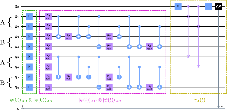
Figure 1: Schematic of the quantum circuit for our algorithm for $d=4$. Each colored box corresponds to a stage of the circuit and represents the set of operations in the respective step for the two copies of $q$ qubits. In the first stage, we prepare the initial state of maximum superposition $|\psi(0)\rangle_{AB}$ for both copies of $q=4$ qubits, starting from the state $|0\rangle$ for each qubit. The second stage is used for the efficient state preparation of $|\psi(t)\rangle_{AB}$ for each copy, where the total number of gates, including both copies, is given by $\frac{3}{2}q^{2}+2q$. In the last stage, with the aid of an ancilla qubit $q_{0}$, we apply the gates corresponding to the variation of the SWAP test to extract the reduced purity $\gamma_{A}(t)$ after executing the circuit several times.

Simulations.— To evaluate the applicability of our algorithm, simulations were performed using IBM’s Qiskit framework (version 0.45.1). These simulations targeted three distinct values of $d$, with results depicted in blue in Fig. 2. For all the simulations, we used $10^{5}$ shots and fixed $\omega=0.1\,\text{s}^{-1}$, as changing the value of $\omega$ has no effect on the Fourier modes $\alpha_{n}$. Regarding the number of executions $p$ of the circuit, we selected $p=375$, $p=1500$, and $p=6000$ for the dimensions $d=16$, $d=32$, and $d=64$, respectively. The values of $p$ were chosen to achieve roughly the same accuracy for the three values of $d$. Using Python (version 3.11.3) with the Scipy library (version 1.11.3), Fourier modes $\alpha_{n}$ were calculated with Simpson’s rule for the numerical integration of Eq. (19). Due to the substantial size of the quantum circuit for the three dimensions analyzed in our simulations, we present the circuit for a lower dimension, $d=4$, purely for illustrative purposes. This simplified example is shown in Fig. 1, allowing us to convey the structure without the complexity of the larger dimensions.

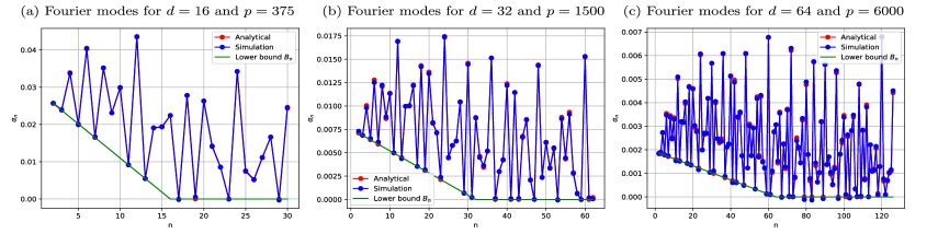
Figure 2: Comparison of simulation results with theoretical predictions for the Fourier modes of the reduced purity across different dimensions $(d=16,32,64)$. Red points represent the analytical values of $\alpha_{n}$, calculated directly from their theoretical expressions, while the green line stands for the minimum value for the Fourier modes, also derived from theoretical calculations. Blue points illustrate the Fourier modes obtained through numerical integration of the reduced purity $\gamma_{A}(t)$ extracted from the classical emulation of our quantum circuit. The numerical integration was performed using various partition values $(p=375,1500,6000)$. Prime numbers are expected to align with the lower bound $B_{n}$, whereas composite numbers appear above. Points closely approaching the lower bound $B_{n}$, yet not precisely on it, may be considered prime candidates, subject to verification due to the presence of statistical error.

Conclusions.— This work presents a qubit-based quantum algorithm for prime number identification, rooted in the analysis of entangled subsystem dynamics. By strategically selecting a bipartite Hamiltonian of dimension $d^{2}$ characterized by energy quantization, we demonstrate that the Fourier modes $\alpha_{n}$ of the reduced purity display distinctive patterns. These patterns enable the differentiation between prime and composite numbers for any integer $n$ such that $1\leq n\leq 2(d-1)$. To implement this protocol as an algorithm for qubit-based quantum computing, we map this $2$-qudit system into a $q$-qubit system using the expression $d^{2}=2^{q}$. In this mapping, as an independent result, we found that the local unitary gates with the form of Eq. (2) may be implemented in polynomial time using the method of Ref. welch .

Executing our quantum circuit involves three stages, as illustrated in Fig. 1: preparation of the initial state $|\psi(0)\rangle_{AB}$ for both sets of $q$ qubits, preparation of the evolved state $|\psi(t)\rangle_{AB}$ also for both sets, and estimating the reduced purity $\gamma_{A}(t)$. These stages have respective gate costs: $2G_{1}=2q$, $2G_{2}(q)=\frac{3}{2}q^{2}+q$, and $G_{3}=\frac{3}{2}q+2$. In particular, $G_{2}(q)$ represents the number of gates necessary to implement local unitary gates that share the same mathematical structure as $\hat{U}(t)$, where this implementation is accomplished using the methodology outlined in Ref. welch . Contrary to the anticipated exponential cost of the method delineated in that work, we have demonstrated that $G_{2}(q)$ scales polynomially with the number of qubits $q$, thereby affirming the high efficiency of that method in preparing the class of states $|\psi(t)\rangle_{AB}$, as defined by Eq. (3). Thus, the total gate cost $G(q)$ for one execution of our quantum circuit is given by $G(q)=\frac{3}{2}q^{2}+\frac{11}{2}q+2$. By defining $N=2(d-1)$ and using $2^{q}=d^{2}$, we find that the asymptotic gate cost is $\mathcal{O}(\log^{2}_{10}(N))$, indicating a quadratic scaling in the number of digits of $N$.

Naturally, although this work presented ideal classical simulations, our algorithm could be implemented on quantum hardware. One major challenge that may arise, however, is that controlled-NOT and SWAP gates require good connectivity between the qubits, which is not always available in existing superconducting qubit-based quantum computers. A simple solution is to explore alternative quantum computing technologies. Trapped ion quantum computers, exemplified by those developed by IonQ and Quantinuum, offer extended coherence times and all-to-all connectivity between qubits, allowing for more effective implementation of these gates. Another approach would be to individually modify the last two stages. For the second stage, which involves preparing $|\psi(t)\rangle_{AB}$ for both copies, alternative methods could be considered, although we suspect that Ref. welch provides the most efficient technique for this purpose. For the third and final stage, since the reduced purity $\gamma_{A}(t)$ is related to the reduced density operator $\hat{\rho}_{A}(t)$, we could replace the direct measurement of $\gamma_{A}(t)$ with a state tomography of $\hat{\rho}_{A}(t)$. Modern tomographic methods, such as classical shadows tomography Aaronson2018 ; Huang2020 ; Nguyen2022 ; Bu2024 , show promise and can be employed for the estimation of $\gamma_{A}(t)$, requiring only $q$ qubits instead of $2q+1$.

Importantly, our demonstration that the unitary gate $\hat{U}(t)$ can be implemented with a polynomial number of gates, contrary to the general expectation of exponential gate requirements, paves the way for the efficient realization of similar transformations in quantum computing. This finding not only enhances the feasibility of executing our prime number identification algorithm on actual quantum systems but also suggests a broader applicability for optimizing other quantum algorithms. As quantum computing continues to evolve, the adaptation of such efficient unitary operations will be crucial in overcoming the limitations posed by gate complexities and in harnessing the full potential of quantum technologies. With advancements in fault tolerance and increased access to a larger number of qubits in the future, our algorithm holds the potential to verify the primality of significantly larger primes, marking a significant step forward in the practical application of quantum algorithms for fundamental computational problems.

In this Supplemental Material, we provide proofs concerning the polynomial efficiency of implementing the diagonal unitary operation $\hat{U}(t)$ Bullock2004_sm , based on the algorithm outlined in Ref. welch_sm , as well as the estimation of the reduced purity $\gamma_{A}(t)$ using the protocol introduced in Ref. ekert_sm . We organize the material into two main sections.

In the first section, we begin with a succinct overview of the algorithm from Ref. welch_sm , focusing on the implementation of diagonal unitary gates. This is followed by the subdivision of the section into three subsections. The first subsection offers a proof of an identity pertaining to Pauli $Z$ gates and controlled-NOT staircases. Subsequently, we present a proposition outlining a general method for obtaining any row of the Paley-ordered Walsh matrices $w_{(.,.)}$ Walsh1923_sm ; Fine1949_sm ; Zhihua1983_sm ; Yuen1975_sm ; Beauchamp1984_sm ; Edwards1975_sm . The third subsection contains two additional results: a theorem concerning the identification of all non-zero Walsh angles $a_{j}(t)$ for $\hat{U}(t)$ along with their respective formulas, and a lemma demonstrating the polynomial gate cost for implementing $\hat{U}(t)$.

The second section is dedicated to the second proof, which is a practical demonstration illustrating how the proposed quantum circuit directly yields the reduced purity $\gamma_{A}(t)$.

I Diagonal unitary gate implementation using Walsh functions

In this section, we provide an overview of the algorithm introduced in Ref. welch_sm for implementing local unitary operations on quantum computers. To begin, we establish some definitions. Let $q$ denote the number of qubits, and consider positive integers $j$ and $k$ with binary and dyadic representations given by

$$\text{bin}(j)=(j_{q}j_{q-1}\cdots j_{1}),$$ (S1)

$$\text{dyad}(k)=(k_{1}k_{2}\cdots k_{q}),$$ (S2)

where the most significant bit (MSB) is on the left. Henceforth, we assume $j=0,1,\cdots,2^{q}-1$ and $k=0,1,\cdots,2^{q}-1$.

Next, we define the discrete Paley-ordered Walsh functions $w_{jk}$ as

$$w_{jk}=(-1)^{\sum_{i=1}^{q}j_{i}k_{i}}.$$ (S3)

Let us discretize the interval $0\leq x<1$ into points given by

$$x_{k}=\frac{k}{2^{q}}.$$ (S4)

Since the Walsh functions form an orthonormal basis, we can define the Walsh-Fourier transform for a function $f_{k}=f(x_{k})$ as follows:

$$a_{j} =\frac{1}{2^{q}}\sum_{k=0}^{2^{q}-1}f_{k}w_{jk},$$ (S5)

$$f_{k} =\sum_{j=0}^{2^{q}-1}a_{j}w_{jk}.$$ (S6)

In qubit-based quantum computing, the state of $q$ qubits generally takes the form $|\psi\rangle=\sum_{k=0}^{2^{q}-1}c_{k}|k\rangle$, where the computational basis $|k\rangle$ is defined as

$$|k\rangle=|k_{1}k_{2}\cdots k_{q}\rangle,$$ (S7)

with $k$ represented in dyadic form $\operatorname{dyad(k)}=(k_{1}k_{2}\cdots k_{q})$. Now, let us define the unitary operator $\hat{U}=e^{i\hat{f}}$ Nielsen2000_sm , where $\hat{f}$ is a diagonal operator in the computational basis:

$$\hat{f}|k\rangle=f_{k}|k\rangle.$$ (S8)

Walsh operators $\{\hat{w}_{j}\}_{j=0}^{2^{q}-1}$ acting on $q$ qubits are naturally defined as

$$\hat{w}_{j}=(\hat{Z_{1}})^{j_{1}}\otimes(\hat{Z_{2}})^{j_{2}}\otimes\cdots\otimes(\hat{Z_{q}})^{j_{q}},$$ (S9)

where $(\hat{Z}_{i})^{1}=\hat{Z}_{i}$ represents the Pauli $Z$ operator and $(\hat{Z}_{i})^{0}=\hat{I}$ denotes the identity matrix, both acting on the $i$-th qubit $q_{i}$. This definition of Walsh operators is advantageous because their action on the computational basis is given by

$$\hat{w}_{j}|k\rangle=w_{jk}|k\rangle.$$ (S10)

This implies that the eigenvalues of Walsh operators $\hat{w}_{j}$ are the Walsh functions $w_{jk}$, and these operators form a basis for diagonal operators $\hat{f}$. Additionally, due to their form, Walsh operators commute. Therefore, considering $\hat{w}_{0}=\hat{I}$, we can disregard $j=0$, leading to the expression

$$\hat{U}=e^{i\hat{f}}=\prod_{j=1}^{2^{q}-1}e^{ia_{j}\hat{w}_{j}}.$$ (S11)

In essence, to apply the method outlined in Ref. welch_sm , we begin by determining the $f_{k}$ values associated with the unitary gate $\hat{U}$. Subsequently, we construct the Walsh functions $w_{jk}$ using the procedure described in Sec. I.2. With these components in hand, Eq. (S5) allows us to compute the Walsh angles $a_{j}$. Finally, utilizing the identity presented in Sec. I.1 to construct the $\hat{w}_{j}$ operators in Eq. (S11) yields the desired unitary $\hat{U}$ with a gate cost of $\mathcal{O}(2^{q})$ in general. This gate cost can be optimized by reordering the commuting exponential operators in Eq. (S11) using the Gray code. It is important to note that even with optimal construction, the quantum circuit for this method typically requires $\mathcal{O}(2^{q})$ gates. However, as we will demonstrate in Sec. I.3, for the specific case of the $q$-qubit unitary gate $\hat{U}(t)$ described in Eq. (2), implementation with a polynomial gate cost is achievable by identifying the null Walsh angles $a_{j}(t)$.

I.1 Relation between Pauli Z gates and CNOTs staircases

In this subsection, we delve into a fundamental identity pivotal to our analysis, which concerns the tensor product of Pauli $\hat{Z}$ operators. This identity plays a crucial role in simplifying the representation of quantum states and operations within our framework. To lay the groundwork for our discussion, we introduce essential notation and concepts:
- $h_{j}$, the Hamming weight of $j$, represents the number of $1$’s in the binary representation of $j$, corresponding to the number of $\hat{Z}$ operators in the tensor product.
- The identity operator $\hat{I}^{\otimes r}$ acts on $r$ qubits, serving as a placeholder in tensor products where no operation is performed.
- The operators $\hat{A}_{h_{j}}$ are constructed from a sequence of controlled-NOT ( $\widehat{CNOT}$ ) gates, defined as $\hat{A}_{h_{j}}=\widehat{CNOT}_{h_{j}}^{1}\widehat{CNOT}_{h_{j}}^{2}\cdots\widehat{CNOT}_{h_{j}}^{h_{j}-1}$, where $\widehat{CNOT}_{b}^{a}$ denotes a $\widehat{CNOT}$ gate with qubit $q_{a}$ as the control and qubit $q_{b}$ as the target.

With these definitions in place, we establish the following identity:

$$\hat{Z}_{1}\otimes\hat{Z}_{2}\otimes\cdots\otimes\hat{Z}_{h_{j}-1}\otimes\hat{Z}_{h_{j}}=\hat{A}_{h_{j}}\left(\hat{I}^{\otimes(h_{j}-1)}\otimes\hat{Z}\right)\hat{A}_{h_{j}}^{-1}$$ (S12)

This identity demonstrates how a tensor product of $\hat{Z}$ operators can be equivalently expressed through a transformation involving $\hat{A}_{h_{j}}$ and its inverse, significantly simplifying the representation and manipulation of such operations. Building upon this foundation, we further examine its implications in the exponential form:

$$e^{ia_{j}\left(\hat{Z}_{1}\otimes\hat{Z}_{2}\otimes\cdots\otimes\hat{Z}_{h_{j}-1}\otimes\hat{Z}_{h_{j}}\right)}=\hat{A}_{h_{j}}\left(\hat{I}^{\otimes(h_{j}-1)}\otimes e^{ia_{j}\hat{Z}}\right)\hat{A}_{h_{j}}^{-1}$$ (S13)

This expression further underscores the utility of the $\hat{A}_{h_{j}}$ transformation in facilitating the implementation of the exponential quantum gates $e^{ia_{j}\hat{w}_{j}}$.

Now, we proceed with the proofs. For the calculations below, unless otherwise convenient, we do not specify the qubit index $i$ of Pauli operators $\hat{Z}_{i}$ or any other operators. We start by rewriting the left side of Eq. (S12) using the projectors $\hat{\Pi}_{0}=|0\rangle\langle 0|$ and $\hat{\Pi}_{1}=|1\rangle\langle 1|$:

$$\hat{Z}\otimes\hat{Z}\otimes\cdots\otimes\hat{Z}\otimes\hat{Z} =(\hat{\Pi}_{0}-\hat{\Pi}_{1})\otimes(\hat{\Pi}_{0}-\hat{\Pi}_{1})\otimes\cdots\otimes(\hat{\Pi}_{0}-\hat{\Pi}_{1})\otimes\hat{Z}$$

$$=\sum_{\operatorname{bin(s)}}(-1)^{h_{s}}\hat{\Pi}_{s_{1}}\otimes\hat{\Pi}_{s_{2}}\otimes\cdots\otimes\hat{\Pi}_{s_{(h_{j}-1)}}\otimes\hat{Z}$$

$$=\sum_{\begin{subarray}{c}\operatorname{bin(s)}\\ h_{s}\text{ even}\end{subarray}}\hat{\Pi}_{s_{1}}\otimes\hat{\Pi}_{s_{2}}\otimes\cdots\otimes\hat{\Pi}_{s_{(h_{j}-1)}}\otimes\hat{Z}-\sum_{\begin{subarray}{c}\operatorname{bin(s)}\\ h_{s}\text{ odd}\end{subarray}}\hat{\Pi}_{s_{1}}\otimes\hat{\Pi}_{s_{2}}\otimes\cdots\otimes\hat{\Pi}_{s_{(h_{j}-1)}}\otimes\hat{Z},$$ (S14)

where the sum on $\operatorname{bin(s)}$ concerns all the possible binary representations $\operatorname{bin(s)}=(s_{(h_{j}-1)}s_{(h_{j}-2)}\cdots s_{1})$ of $h_{j}-1$ bits. It will be helpful to define

$$\Sigma_{\text{even}} =\sum_{\begin{subarray}{c}\operatorname{bin(s)}\\ h_{s}\text{ even}\end{subarray}}\hat{\Pi}_{s_{1}}\otimes\hat{\Pi}_{s_{2}}\otimes\cdots\otimes\hat{\Pi}_{s_{(h_{j}-1)}},$$ (S15)

$$\Sigma_{\text{odd}} =\sum_{\begin{subarray}{c}\operatorname{bin(s)}\\ h_{s}\text{ odd}\end{subarray}}\hat{\Pi}_{s_{1}}\otimes\hat{\Pi}_{s_{2}}\otimes\cdots\otimes\hat{\Pi}_{s_{(h_{j}-1)}}.$$ (S16)

For these two definitions, the following relations are inherited from the projectors:

$$\Sigma_{\text{even}}\Sigma_{\text{even}}=\Sigma_{\text{even}},$$ (S17)

$$\Sigma_{\text{odd}}\Sigma_{\text{odd}}=\Sigma_{\text{odd}},$$ (S18)

$$\Sigma_{\text{even}}\Sigma_{\text{odd}}=\Sigma_{\text{odd}}\Sigma_{\text{even}}=0.$$ (S19)

Therefore, after defining $\hat{I}$ as the identity gate acting on a single qubit and recalling that $\hat{X}\hat{Z}\hat{X}=-\hat{Z}$, we obtain:

$$\hat{Z}\otimes\hat{Z}\otimes\cdots\otimes\hat{Z}\otimes\hat{Z} =\Sigma_{\text{even}}\otimes\hat{Z}-\Sigma_{\text{odd}}\otimes\hat{Z}$$

$$=\Sigma_{\text{even}}\otimes\hat{Z}+\Sigma_{\text{odd}}\otimes\hat{X}\hat{Z}\hat{X}$$

$$=\left(\Sigma_{\text{even}}\otimes\hat{I}\right)\left(\hat{I}^{\otimes(h_{j}-1)}\otimes\hat{Z}\right)\left(\Sigma_{\text{even}}\otimes\hat{I}\right)+\left(\Sigma_{\text{odd}}\otimes\hat{X}\right)\left(\hat{I}^{\otimes(h_{j}-1)}\otimes\hat{Z}\right)\left(\Sigma_{\text{odd}}\otimes\hat{X}\right)$$

$$=\left(\Sigma_{\text{even}}\otimes\hat{I}\right)\left(\hat{I}^{\otimes(h_{j}-1)}\otimes\hat{Z}\right)\left(\Sigma_{\text{even}}\otimes\hat{I}\right)+\left(\Sigma_{\text{odd}}\otimes\hat{X}\right)\left(\hat{I}^{\otimes(h_{j}-1)}\otimes\hat{Z}\right)\left(\Sigma_{\text{odd}}\otimes\hat{X}\right)$$

$$\quad+\left(\Sigma_{\text{odd}}\otimes\hat{X}\right)\left(\hat{I}^{\otimes(h_{j}-1)}\otimes\hat{Z}\right)\left(\Sigma_{\text{even}}\otimes\hat{I}\right)+\left(\Sigma_{\text{even}}\otimes\hat{I}\right)\left(\hat{I}^{\otimes(h_{j}-1)}\otimes\hat{Z}\right)\left(\Sigma_{\text{odd}}\otimes\hat{X}\right)$$

$$=\left(\Sigma_{\text{even}}\otimes\hat{I}+\Sigma_{\text{odd}}\otimes\hat{X}\right)\left(\hat{I}^{\otimes(h_{j}-1)}\otimes\hat{Z}\right)\left(\Sigma_{\text{even}}\otimes\hat{I}+\Sigma_{\text{odd}}\otimes\hat{X}\right).$$ (S20)

To continue, we examine the product of two controlled-NOT gates targeting the same qubit:

$$\widehat{CNOT}_{3}^{1}\widehat{CNOT}_{3}^{2} =\left(\hat{\Pi}_{0}\otimes\hat{I}\otimes\hat{I}+\hat{\Pi}_{1}\otimes\hat{I}\otimes\hat{X}\right)\left(\hat{I}\otimes\hat{\Pi}_{0}\otimes\hat{I}+\hat{I}\otimes\hat{\Pi}_{1}\otimes\hat{X}\right)$$

$$=\hat{\Pi}_{0}\otimes\hat{\Pi}_{0}\otimes\hat{I}+\hat{\Pi}_{0}\otimes\hat{\Pi}_{1}\otimes\hat{X}+\hat{\Pi}_{1}\otimes\hat{\Pi}_{0}\otimes\hat{X}+\hat{\Pi}_{1}\otimes\hat{\Pi}_{1}\otimes\hat{I}$$

$$=\left(\hat{\Pi}_{0}\otimes\hat{\Pi}_{0}+\hat{\Pi}_{1}\otimes\hat{\Pi}_{1}\right)\otimes\hat{I}+\left(\hat{\Pi}_{1}\otimes\hat{\Pi}_{0}+\hat{\Pi}_{0}\otimes\hat{\Pi}_{1}\right)\otimes\hat{X}.$$

The equation above suggests a similar form for a more general case. In fact, it holds that

$$\hat{A}_{h_{j}} =\widehat{CNOT}_{h_{j}}^{1}\widehat{CNOT}_{h_{j}}^{2}\cdots\widehat{CNOT}_{h_{j}}^{h_{j}-1}$$

$$=\sum_{\begin{subarray}{c}\operatorname{bin(s)}\\ h_{s}\text{ even}\end{subarray}}\hat{\Pi}_{s_{1}}\otimes\hat{\Pi}_{s_{2}}\otimes\cdots\otimes\hat{\Pi}_{s_{(h_{j}-1)}}\otimes\hat{I}+\sum_{\begin{subarray}{c}\operatorname{bin(s)}\\ h_{s}\text{ odd}\end{subarray}}\hat{\Pi}_{s_{1}}\otimes\hat{\Pi}_{s_{2}}\otimes\cdots\otimes\hat{\Pi}_{s_{(h_{j}-1)}}\otimes\hat{X}$$

$$=\Sigma_{\text{even}}\otimes\hat{I}+\Sigma_{\text{odd}}\otimes\hat{X}.\$$ (S22)

Then, because $\hat{A}_{h_{j}}^{-1}=\hat{A}_{h_{j}}$, we obtain the proposed expression (S12) by using the identity (S22) on Eq. (S20):

$$\hat{Z}_{1}\otimes\hat{Z}_{2}\otimes\cdots\otimes\hat{Z}_{h_{j}-1}\otimes\hat{Z}_{h_{j}}=\hat{A}_{h_{j}}\left(\hat{I}^{\otimes(h_{j}-1)}\otimes\hat{Z}\right)\hat{A}_{h_{j}}^{-1}.$$ (S23)

Using this result, we can further demonstrate the validity of Eq. (S13):

$$e^{ia_{j}\left(\hat{Z}_{1}\otimes\hat{Z}_{2}\otimes\cdots\otimes\hat{Z}_{h_{j}-1}\otimes\hat{Z}_{h_{j}}\right)} =\sum_{n=0}^{\infty}\frac{\left(ia_{j}\right)^{n}}{n!}\left(\hat{Z}\otimes\hat{Z}\otimes\cdots\otimes\hat{Z}\right)^{n}$$

$$=\sum_{n=0}^{\infty}\frac{\left(ia_{j}\right)^{n}}{n!}\left(\hat{A}_{h_{j}}\left(\hat{I}^{\otimes(h_{j}-1)}\otimes\hat{Z}\right)\hat{A}_{h_{j}}^{-1}\right)^{n}$$

$$=\sum_{n=0}^{\infty}\frac{\left(ia_{j}\right)^{n}}{n!}\hat{A}_{h_{j}}\left(\hat{I}^{\otimes(h_{j}-1)}\otimes\hat{Z}^{n}\right)\hat{A}_{h_{j}}^{-1}$$

$$=\hat{A}_{h_{j}}\left(\hat{I}^{\otimes(h_{j}-1)}\otimes\sum_{n=0}^{\infty}\frac{\left(ia_{j}\hat{Z}\right)^{n}}{n!}\right)\hat{A}_{h_{j}}^{-1}$$

$$=\hat{A}_{h_{j}}\left(\hat{I}^{\otimes(h_{j}-1)}\otimes e^{ia_{j}\hat{Z}}\right)\hat{A}_{h_{j}}^{-1}.$$ (S24)

In this context, we revisit the formulation of Walsh operators, as delineated in Eq. (S9), represented by $\hat{w}_{j}=(\hat{Z_{1}})^{j_{1}}\otimes(\hat{Z_{2}})^{j_{2}}\otimes\cdots\otimes(\hat{Z_{q}})^{j_{q}}$, where the action of $e^{ia_{j}\hat{w}_{j}}$ on a $q$-qubit basis state $|k\rangle=|k_{1}k_{2}\cdots k_{q}\rangle$ is considered. To elaborate on the analysis, we introduce a strategic reordering of the indices $j_{i}$, segregating them into two distinct sets: the first, denoted by $\{m_{i}\}_{i=1}^{h_{j}}$, corresponds to indices where $j_{m_{i}}=1$, spanning the initial $h_{j}$ bits; the latter set, $\{m_{i}\}_{i=h_{j}+1}^{q}$, encompasses indices with $j_{m_{i}}=0$, accounting for the remaining $q-h_{j}$ bits. The accordingly reconfigured states of qubits $q_{i}$ and the operators $(\hat{Z}_{i})^{j_{i}}$ can be achieved by applying SWAP gates. This culminates in the revised Walsh operator $\hat{\Omega}_{j}$ and revised basis state $|k^{\prime}\rangle$, articulated as:

$$\hat{\Omega}_{j} =\left(\hat{Z}_{m_{1}}\otimes\hat{Z}_{m_{2}}\otimes\cdots\otimes\hat{Z}_{m_{h_{j}}}\right)\otimes\left(\hat{I}_{m_{h_{j}+1}}\otimes\hat{I}_{m_{h_{j}+2}}\otimes\cdots\otimes\hat{I}_{m_{q}}\right),$$ (S25)

$$|k^{\prime}\rangle =|k_{m_{1}}k_{m_{2}}\cdots k_{m_{q}}\rangle.$$ (S26)

Leveraging Eq. (S24), we have

$$e^{ia_{j}\hat{\Omega}_{j}}|k^{\prime}\rangle =e^{ia_{j}\left(\hat{Z}_{m_{1}}\otimes\hat{Z}_{m_{2}}\otimes\cdots\otimes\hat{Z}_{m_{h_{j}}}\right)\otimes\left(\hat{I}_{m_{h_{j}+1}}\otimes\hat{I}_{m_{h_{j}+2}}\otimes\cdots\otimes\hat{I}_{m_{q}}\right)}|k_{m_{1}}k_{m_{2}}\cdots k_{m_{q}}\rangle$$

$$=e^{ia_{j}\left(\hat{Z}_{m_{1}}\otimes\hat{Z}_{m_{2}}\otimes\cdots\otimes\hat{Z}_{m_{h_{j}}}\right)}\otimes\left(\hat{I}_{m_{h_{j}+1}}\otimes\hat{I}_{m_{h_{j}+2}}\otimes\cdots\otimes\hat{I}_{m_{q}}\right)|k_{m_{1}}k_{m_{2}}\cdots k_{m_{q}}\rangle$$

$$=\left[\hat{A}_{h_{j}}\left(\hat{I}^{\otimes(h_{j}-1)}\otimes e^{ia_{j}\hat{Z}}\right)\hat{A}_{h_{j}}^{-1}\right]\otimes\hat{I}^{\otimes(q-h_{j})}|k_{m_{1}}k_{m_{2}}\cdots k_{m_{q}}\rangle.$$ (S27)

As it was stated previously, our objective lies in the action of the original operator $e^{ia_{j}\hat{w}_{j}}$ on the original basis state $|k\rangle$, i.e., $e^{ia_{j}\hat{w}_{j}}|k\rangle$. However, through the application of the same SWAP gates used before to Eq. (S27), we restore the original sequence of qubits and Pauli operators, thereby preserving the structural integrity of the action of the operator $e^{ia_{j}\hat{w}_{j}}$ on the basis state $|k\rangle$.

I.2 Walsh matrices construction

A well-established result in the literature states that any discrete Walsh function $w_{jk}$ can be represented as a product of Rademacher functions, with the exception of $w_{0k}$, which trivially remains a constant function $w_{0k}=1$. Rademacher functions, denoted as $w_{l_{r}k}$, are Walsh functions where $l_{r}$ is a power of 2, specifically $l_{r}=2^{(r-1)}$.

To illustrate, consider a Walsh matrix $w_{(.,.)}$, where $w_{jk}=w_{(j,k)}$, representing Paley-ordered Walsh functions arranged in a square matrix of dimensions $2^{q}\times 2^{q}$. In matrix formalism, any row $w_{(j,.)}$ can be understood as the column-wise product of corresponding $h_{j}$ Rademacher rows $\{w_{({l_{m_{i}}},.)}\}_{i=1}^{h_{j}}$, organized by ascending order of magnitude $l_{m_{1}}<l_{m_{2}}<\cdots<l_{m_{h_{j}}}$. Here, $h_{j}$ signifies the Hamming weight of $j$. The Rademacher rows $w_{({l_{m_{i}}},.)}$ satisfy $j=\sum_{i=1}^{h_{j}}l_{m_{i}}=\sum_{i=1}^{h_{j}}2^{(m_{i}-1)}$.

Here, we introduce this result as a proposition with minor adjustments. This adaptation enables us to introduce the required notation for the theorem detailed in the subsequent subsection, which concerns the implementation of $\hat{U}(t)$. Consistent with convention, we index the rows and columns of our Walsh matrix starting from $0$, with the maximum index value being $2^{q}-1$.

Proposition 1.

Consider a positive integer $r$ satisfying $1\leq r\leq q$, where $l_{r}=2^{(r-1)}$. Let $\{m_{i}\}_{i=1}^{h_{j}}$ be a sequence of integers in increasing order of magnitude and let $j$ be any row index of the $2^{q}\times 2^{q}$ Walsh matrix $w_{(.,.)}$. Then, the row $w_{(j,.)}$ will satisfy only one of the following statements:

1. If $j=l_{r}$, then the Rademacher row $w_{(j,.)}=w_{(l_{r},.)}$ of the Walsh matrix is given by

   $$w_{(l_{r},.)}=\bigl{[}(R_{r})(-R_{r})(R_{r})(-R_{r})\cdots(R_{r})(-R_{r})\bigr{]},$$ (S28)

   where $R_{r}=(+1)(\times T_{r})$ is a row of length $T_{r}=2^{(q-r)}$ and $T_{r}$ is called the period of the row $w_{(l_{r},.)}$. The notation means that $w_{(l_{r},.)}$ is composed of sign alternating sequences of $T_{r}$ elements. These sequences are $R_{r}$ and $-R_{r}$ and all their elements are, respectively, equal to $+1$ and $-1$.

2. If $j\neq l_{r}$, we define $j=\sum_{i=1}^{h_{j}}l_{m_{i}}=\sum_{i=1}^{h_{j}}2^{(m_{i}-1)}$, then the row $w_{(j,.)}$ of the Walsh matrix is given by

   $$w_{(j,.)}=\bigl{[}(R_{m_{1}})(-R_{m_{1}})(R_{m_{1}})(-R_{m_{1}})\cdots(R_{m_{1}})(-R_{m_{1}})\bigr{]},$$ (S29)

   where $R_{m_{1}}$ is obtained from the recursive relation

   $$R_{m_{(i-1)}}=\bigl{[}(R_{m_{i}})(-R_{m_{i}})(R_{m_{i}})(-R_{m_{i}})\cdots(R_{m_{i}})(-R_{m_{i}})\bigr{]},$$ (S30)

   with $R_{m_{0}}=w_{(j,.)}$ and $R_{m_{h_{j}}}=(+1)(\times T_{m_{h_{j}}})$. Each $R_{m_{i}}$, for $1\leq i\leq h_{j}$, is a row of length $T_{m_{i}}=2^{(q-m_{i})}$.

Proof.

We shall prove each case of Proposition 1 separately.

1. Case $j=l_{r}$. The binary representation of $j=l_{r}=2^{(r-1)}$ is given by

$$\operatorname{bin(j)}=(000\cdots 01_{r}0\cdots 000),$$ (S31)

where we have introduced the notation $1_{r}=j_{r}=1$ to make it clear that the only non-zero binary element of $\operatorname{bin(j)}$ is in the position $r$.

Definition 1.

We define the exponent $S(j,k)$ of Eq. $(\ref{walsh_functions})$ as

$$S(j,k)=\sum_{i=1}^{q}j_{i}k_{i}.$$ (S32)

If $S(j,k)$ is even, then $w_{(j,k)}=1$. If $S(j,k)$ is odd, then $w_{(j,k)}=-1$.

Then, for any $0\leq k\leq 2^{q}-1$, we have

$$k_{r} =0\implies S(j,k)=j_{r}k_{r}=\operatorname{even},$$ (S33)

$$k_{r} =1\implies S(j,k)=j_{r}k_{r}=\operatorname{odd.}$$ (S34)

Now, we consider only a partial dyadic representation string $\operatorname{dyad_{r}(k)}$ of $k$. Since the dyadic string of $k$ is the same as its reverse binary string, a partial dyadic string up to the position $r$ is defined as

$$\operatorname{dyad_{r}(k)}=(k_{r}k_{r+1}\cdots k_{(q-1)}k_{q}).$$ (S35)

There are $q-r+1$ entries in the partial dyadic string of Eq. (S35), resulting in a total of $2^{(q-r+1)}$ combinations. The first half of these combinations corresponds to $k_{r}=0$ and the second half corresponds to $k_{r}=1$. That is, the first $2^{(q-r)}$ elements of $S(j,.)$ are even and the next $2^{(q-r)}$ elements of $S(j,.)$ are odd. Note that we did not consider the other $r-1$ entries that show up in the complete dyadic string $\operatorname{dyad(k)}$ of $k$. This is justified by the fact that the pattern we just described will remain true for any configuration of the disregarded $r-1$ entries, as changing any of these entries allows another total of $2^{(q-r+1)}$ possible combinations with the same pattern for $\operatorname{dyad_{r}(k)}$. From this, we infer that $S(j,.)$ is completely defined by alternating sequences of even and odd elements, with each sequence having length $T_{r}=2^{(q-r)}$. Thus, using that $w_{(j,k)}=(-1)^{S(j,k)}$, the Rademacher row $w_{(j,.)}=w_{(l_{r},.)}$ will be given by

$$w_{(l_{r},.)}=\bigl{[}(R_{r})(-R_{r})(R_{r})(-R_{r})\cdots(R_{r})(-R_{r})\bigr{]},$$ (S36)

with $R_{r}=(+1)(\times T_{r})$ and period $T_{r}=2^{(q-r)}$.

2. Case $j\neq l_{r}$. Even though $j$ here cannot be written as a power of $2$, it can always be written as a sum of these powers:

$$j=\sum_{i=1}^{h_{j}}l_{m_{i}}=\sum_{i=1}^{h_{j}}2^{(m_{i}-1)},$$ (S37)

and we conveniently choose the indices $m_{i}$ to match the positions of the non-zero binary elements of $j$, i.e., $j_{m_{i}}=1$. That is, if we consider only the non-zero binary elements $\operatorname{bin_{\neq 0}(j)}$ of the binary representation $\operatorname{bin(j)}$ of $j$, then

$$\operatorname{bin_{\neq 0}(j)}=(j_{m_{h_{j}}}\cdots j_{m_{2}}j_{m_{1}}).$$ (S38)

Thus, for any $0\leq k\leq 2^{q}-1$ we have

$$S(j,k)=\sum_{i=1}^{q}j_{i}k_{i}=\sum_{i=1}^{h_{j}}j_{m_{i}}k_{m_{i}}.$$ (S39)

Because each term $j_{m_{i}}k_{m_{i}}$ in the sum above is the corresponding $l_{m_{i}}$ term $S(l_{m_{i}},k)$, it must be true that

$$w_{(j,k)} =(-1)^{\sum_{i=1}^{h_{j}}S(l_{m_{i}},k)}$$

$$=\prod_{i=1}^{h_{j}}(-1)^{S(l_{m_{i}},k)}$$

$$=\prod_{i=1}^{h_{j}}w_{(l_{m_{i}},k)}.$$ (S40)

Eq. (S40) means that any row $w_{(j,)}$ is the column-wise product of the corresponding Rademacher rows $w_{(l_{m_{i}},.)}$ such that $j=\sum_{i=1}^{h_{j}}l_{m_{i}}$.

Since $l_{m_{1}}<l_{m_{2}}<\cdots<l_{m_{h_{j}}}$, the respective periods $T_{m_{i}}=2^{(q-m_{i})}$, for $1\leq i\leq h_{j}$, must obey $T_{m_{1}}>T_{m_{2}}>\cdots>T_{m_{h_{j}}}$. We know that for $0\leq k\leq T_{m_{1}}-1$, we have $w_{(l_{m_{1}},k)}=+1$. Then, if $0\leq k\leq T_{m_{1}}-1$, the elements $w_{(j,k)}$ of Eq. (S40) can be written as $w_{(j,k)}=\prod_{i=2}^{h_{j}}w_{(l_{m_{i}},k)}$. Now, any Rademacher row $w_{(l_{m_{i}},.)}$ has a period $T_{m_{i}}$ and thus is composed of alternating pairs of sequences, where each pair is made of a sequence of $T_{m_{i}}$ terms all equal to $+1$ and a sequence of $T_{m_{i}}$ terms all equal to $-1$. This implies that the number of times $L_{[1,i]}$ that we can fit these pairs of $2T_{m_{i}}$ terms into the length of the largest period $T_{m_{1}}$ is given by

$$L_{[1,i]} =\frac{T_{m_{1}}}{2T_{m_{i}}}$$

$$=\frac{2^{(q-m_{1})}}{2\times 2^{(q-m_{i})}}$$

$$=\frac{2^{(m_{i}-m_{1})}}{2}$$

$$=\frac{l_{m_{i}}}{2l_{m_{1}}},$$ (S41)

which evidently shows, for $i\geq 2$, that $L_{[1,i]}$ is an integer, specifically, a power of $2$. Now, for $T_{m_{1}}\leq k\leq 2T_{m_{1}}-1$ we must have $w_{(l_{m_{1}},k)}=-1$ , and the pattern of $w_{(j,.)}$ will occur again for these next $T_{m_{1}}$ values of $k$, except that in this case we get a sign change, i.e., $w_{(j,k)}=-\prod_{i=2}^{h_{j}}w_{(l_{m_{i}},k)}$. After these first $2T_{m_{1}}$ terms, the periodicity of $w_{(l_{m_{1},.)}}$ implies that the aforementioned pattern will continue to repeat itself until we have the row $w_{(j,.)}$ completely filled. From that, we conclude that $T_{m_{1}}$ is a common period for every composing Rademacher row of $w_{(j,.)}$. We can also analyze how many pairs of $2T_{m_{i}}$ terms fit into the length of any other period $T_{m_{i^{\prime}}}>T_{m_{i}}$, that is, calculate the expression for $L_{[i^{\prime},i]}$. In this case, for any $i>i^{\prime}$, we have

$$L_{[i^{\prime},i]} =\frac{T_{m_{i^{\prime}}}}{2T_{m_{i}}}$$

$$=\frac{2^{(q-m_{i^{\prime}})}}{2\times 2^{(q-m_{i})}}$$

$$=\frac{2^{(m_{i}-m_{i^{\prime}})}}{2}$$

$$=\frac{l_{m_{i}}}{2l_{m_{i^{\prime}}}}.$$ (S42)

This shows that any period $T_{m_{i^{\prime}}}$, for $h_{j}-1\geq i^{\prime}\geq 1$, has a length that can be perfectly fit by an integer number of pairs of $2T_{m_{i}}$ terms such that $T_{m_{i^{\prime}}}>T_{m_{i}}$. The extreme case of $T_{m_{h_{j}}}$, however, will never have any lower period, a relevant fact that leads to the following definition:

Definition 2.

To proceed, for $1\leq i\leq h_{j}$, we define the recursive relation

$$R_{m_{(i-1)}}=\bigl{[}(R_{m_{i}})(-R_{m_{i}})(R_{m_{i}})(-R_{m_{i}})\cdots(R_{m_{i}})(-R_{m_{i}})\bigr{]},$$ (S43)

where $R_{m_{h_{j}}}=(+1)(\times T_{m_{h_{j}}})$, and $R_{m_{0}}$ and $R_{m_{i}}$ have respective periods $T_{m_{0}}=2^{q}$ and $T_{m_{i}}=2^{(q-m_{i})}$.

Utilizing the recursive relation in Eq. (S43), we demonstrate that $w_{(j,.)}=R_{m_{0}}$. This recursive relation maintains a critical connection with the Rademacher rows $w_{(l_{m_{i}},.)}$. The initial condition $R_{m_{h_{j}}}=(+1)(\times T_{m_{h_{j}}})$ is chosen due to $T_{m_{h_{j}}}$ being the minimal period, thus serving as the recursive sequence’s base case. For periods $T_{m_{(i-1)}}>T_{m_{h_{j}}}$, the sequence iteratively incorporates $R_{m_{i}}$, further integrating the effects of $R_{m_{(i+1)}}$ until the base case $R_{m_{h_{j}}}=(+1)(\times T_{m_{h_{j}}})$ is reached. Particularly, $R_{m_{0}}$ is synthesized through several $(R_{m_{1}})(-R_{m_{1}})$ pairs, effectively encapsulating the periodic characteristics of the composing Rademacher rows of $w_{(j,.)}$. Therefore, each term in the sequence $R_{m_{1}}$ of $T_{m_{1}}$ terms corresponds to either $\prod_{i=2}^{h_{j}}w_{(l_{m_{i}},k)}$ or its negative counterpart, $-\prod_{i=2}^{h_{j}}w_{(l_{m_{i}},k)}$, for the relevant $T_{m_{1}}$ columns $k$. As we have shown, the products $\pm\prod_{i=2}^{h_{j}}w_{(l_{m_{i}},k)}$ fully compose the row $w_{(j,.)}$, leading to the conclusion that $w_{(j.)}=R_{m_{0}}$. Hence, we have:

$$w_{(j,.)}=\bigl{[}(R_{m_{1}})(-R_{m_{1}})(R_{m_{1}})(-R_{m_{1}})\cdots(R_{m_{1}})(-R_{m_{1}})\bigr{]}.$$ (S44)

∎

I.3 Demonstration of polynomial cost

As we have shown in the beginning of this section, to use the method of Ref. welch_sm , we must calculate the Walsh angles $a_{j}$, given by

$$a_{j} =\frac{1}{2^{q}}\sum_{k=0}^{2^{q}-1}f_{k}w_{jk},$$

$$=\frac{1}{2^{q}}[w_{(j,.)}]\times[\vec{f}]^{T},$$ (S45)

where we have introduced the symbol $T$ for transposition, since $\vec{f}$ was originally defined as a row vector. The components $f_{k}$ of $\vec{f}$ are extracted as the eigenvalues of the operator

$$\hat{f}=\sum_{k=0}^{2^{q}-1}f_{k}|k\rangle\langle k|.$$ (S46)

Then, a general unitary operator of the form $\hat{U}=e^{i\hat{f}}$, when represented in the computational basis $|k\rangle$, is given by the following diagonal matrix:

$$U=\begin{bmatrix}D_{1}&0&\cdots&0\\ 0&D_{2}&\cdots&0\\ \vdots&\vdots&\ddots&\vdots\\ 0&0&\cdots&D_{d}\end{bmatrix},$$ (S47)

where $d^{2}=2^{q}$, with $d$ a power of $2$, and the $D_{s}$ are diagonal matrices, for $1\leq s\leq d$. In this paper, we define these diagonal matrices $D_{s}$ as

$$D_{s}=\begin{bmatrix}e^{i\varphi_{s}}&0&\cdots&0\\ 0&e^{2i\varphi_{s}}&\cdots&0\\ \vdots&\vdots&\ddots&\vdots\\ 0&0&\cdots&e^{di\varphi_{s}}\end{bmatrix},$$ (S48)

where $i^{2}=-1$, $\varphi_{s}=s\kappa$ and $\kappa$ is a real number. Comparing with the unitary gate $\hat{U}(t)$ of Eq. (2) for our quantum algorithm, we must use $\kappa=-\omega t$. However, because $\kappa$ is a global factor for $\vec{f}$ and thus a multiplicative factor in the expression for $a_{j}$ in Eq. (I.3), we can choose $\kappa=1$ to facilitate further calculations. The vector $\vec{f}$ that we are going to use is then given by

$$\vec{f}=[(1,2,3,\cdots,d),(2,4,6,\cdots,2d),(3,6,9,\cdots,3d),\cdots,(d,2d,3d,\cdots,d^{2})].$$ (S49)

There is also another global factor $\frac{1}{2^{q}}=\frac{1}{d^{2}}$ in the expression (I.3), which can be equally disregarded in the calculations. Taking into account these two global factors, $a_{j}$ will be redefined to be

$$a_{j}=[w_{(j,.)}]\times[\vec{f}]^{T},$$ (S50)

with $\vec{f}$ given by Eq. (S49). Thus, the relevant Walsh angles $a_{j}(t)$ for $\hat{U}(t)$ should be defined as

$$a_{j}(t)=\frac{-\omega t}{d^{2}}a_{j}.$$ (S51)

Since there is no risk of confusion, $a_{j}$ and $a_{j}(t)$ are both referred to as ‘Walsh angles’ in this work. The following theorem concerns the derivations of the expressions for the non-zero Walsh angles $a_{j}(t)$ corresponding to the unitary gate $\hat{U}(t)$ of Eq. (2). Even though we are using $q$ even here, it should be noted that a similar theorem holds for odd values of $q$, opening possibilities for the efficient implementation of any $2^{q}\times 2^{q}$ diagonal unitary gate $\hat{U}(t)$ with the form of Eq. (2).

Theorem 2.

Let $W$ be the set of non-zero Walsh angles $a_{j}(t)$ for the $q$-qubit unitary gate $\hat{U}(t)$ of Eq. (2), with $q$ even. Then

$$W=W_{1}\cup W_{2},$$ (S52)

with

$$W_{1}=\left\{a_{j}(t)=\begin{cases}\frac{d(1+d)\omega t}{8j}&\text{if $j\leq d/2$},\\ \frac{d^{2}(1+d)\omega t}{8j}&\text{if $j\geq d$},\end{cases}\Big{|}h_{j}=1\right\},$$ (S53)

and

$$W_{2}=\left\{a_{j}(t)=\frac{-d^{3}\omega t}{16l_{m_{1}}l_{m_{2}}}\Big{|}h_{j}=2\text{ and }j=l_{m_{1}}+l_{m_{2}}\text{ for }l_{m_{1}}\leq d/2\text{ and }l_{m_{2}}\geq d\right\},$$ (S54)

where $h_{j}$ is the Hamming weight of $j$ and $d^{2}=2^{q}$.

The quantum circuit corresponding to the implementation of $\hat{U}(t)$ is presented for $d=4$ in Fig. S1. As it is evident, Theorem 2 eliminates the vast majority of the $2^{q}-1$ Walsh angles $a_{j}(t)$ that would be necessary, in general, to implement this type of local unitary gate exactly. In Lemma 3, we show that the number of gates needed to exactly implement $\hat{U}(t)$ is polynomial in the number of qubits $q$.

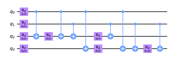
Figure S1: Quantum circuit that implements the local unitary gate $\hat{U}(t)$ for $d=4$. We used the mathematical identity demonstrated in Sec. I.1 to express an exponential of $Z$ Pauli gates as a single $Z$-rotation $\hat{R}_{z}(\theta_{j}(t))$, with the angles given by $\theta_{j}(t)=-2a_{j}(t)$, and several controlled-NOT gates.

In what follows, we list some definitions and their respective properties, in order to use them in the proof of Theorem 2, that will be presented afterwards.

Definition 3.

Elementary vectors are defined as

$$\vec{P_{\eta}}=[\eta,2\eta,3\eta,\cdots,d\eta].$$ (S55)

Definition 4.

Extended vectors are defined as

$$\vec{P}_{\{\alpha|\alpha+\beta\}}=[\vec{P}_{\alpha},\vec{P}_{\alpha+1},\vec{P}_{\alpha+2},\cdots,\vec{P}_{\alpha+\beta}].$$ (S56)

Definition 5.

Partial vectors are defined as

$$\vec{p}^{\,(\eta)}_{\{\alpha|\alpha+\beta\}}=[p^{(\eta)}_{\alpha},p^{(\eta)}_{\alpha+1},p^{(\eta)}_{\alpha+2},\cdots,p^{(\eta)}_{\alpha+\beta}],$$ (S57)

where we defined the notation $\vec{P_{\eta}}=[p^{(\eta)}_{1},p^{(\eta)}_{2},p^{(\eta)}_{3},\cdots,p^{(\eta)}_{d}]$ for elementary vectors.

Property 6.

Using definition (S49) for $\vec{f}$ and definition 3 for $\vec{P}_{\eta}$, we can write

$$\vec{f}=[\vec{P_{1}},\vec{P_{2}},\vec{P_{3}},\cdots,\vec{P_{d}}].$$ (S58)

Property 7.

By the definition 3 for elementary vectors $\vec{P}_{\eta}$, it follows that

$$\vec{P_{\eta}}=\eta\vec{P_{1}}.$$ (S59)

Property 8.

It follows directly from property 7 that

$$\vec{P_{\eta}}-\vec{P}_{\eta+\Delta}=-\Delta\vec{P_{1}}.$$ (S60)

Property 9.

Applying property 8 for each elementary vector of definition 4 gives us

$$\vec{P}_{\{\alpha|\alpha+\beta\}}-\vec{P}_{\{\alpha+\Delta|\alpha+\Delta+\beta\}} =[\vec{P}_{\alpha},\vec{P}_{\alpha+1},\vec{P}_{\alpha+2},\cdots,\vec{P}_{\alpha+\beta}]-[\vec{P}_{\alpha+\Delta},\vec{P}_{\alpha+\Delta+1},\vec{P}_{\alpha+\Delta+2},\cdots,\vec{P}_{\alpha+\Delta+\beta}],$$

$$=[\vec{P}_{\alpha}-\vec{P}_{\alpha+\Delta},\vec{P}_{\alpha+1}-\vec{P}_{\alpha+\Delta+1},\vec{P}_{\alpha+2}-\vec{P}_{\alpha+\Delta+2},\cdots,\vec{P}_{\alpha+\beta}-\vec{P}_{\alpha+\Delta+\beta}],$$

$$=-\Delta[\vec{P}_{1},\vec{P}_{1},\vec{P}_{1},\cdots,\vec{P}_{1}].$$ (S61)

Property 10.

It follows, respectively, from the definition 5 of partial vectors $\vec{p}^{\,(\eta)}_{\{\alpha|\alpha+\beta\}}$, property 7, and definition 3 applied to $\vec{P}_{1}$, that

$$\vec{p}^{\,(\eta)}_{\{\alpha|\alpha+\beta\}}-\vec{p}^{\,(\eta)}_{\{\alpha+\Delta|\alpha+\Delta+\beta\}} =[p^{(\eta)}_{\alpha},p^{(\eta)}_{\alpha+1},p^{(\eta)}_{\alpha+2},\cdots,p^{(\eta)}_{\alpha+\beta}]-[p^{(\eta)}_{\alpha+\Delta},p^{(\eta)}_{\alpha+\Delta+1},p^{(\eta)}_{\alpha+\Delta+2},\cdots,p^{(\eta)}_{\alpha+\Delta+\beta}],$$

$$=[p^{(\eta)}_{\alpha}-p^{(\eta)}_{\alpha+\Delta},p^{(\eta)}_{\alpha+1}-p^{(\eta)}_{\alpha+\Delta+1},p^{(\eta)}_{\alpha+2}-p^{(\eta)}_{\alpha+\Delta+2},\cdots,p^{(\eta)}_{\alpha+\beta}-p^{(\eta)}_{\alpha+\Delta+\beta}],$$

$$=\eta[p^{(1)}_{\alpha}-p^{(1)}_{\alpha+\Delta},p^{(1)}_{\alpha+1}-p^{(1)}_{\alpha+\Delta+1},p^{(1)}_{\alpha+2}-p^{(1)}_{\alpha+\Delta+2},\cdots,p^{(1)}_{\alpha+\beta}-p^{(1)}_{\alpha+\Delta+\beta}],$$

$$=-\eta\Delta[1,1,1,\cdots,1].$$ (S62)

Building upon the definitions and properties outlined earlier, we now introduce an important vector, denoted by $\vec{f}^{\,\sigma}_{m_{i}}$, constructed from components of $\vec{f}$. This vector emerges as a cornerstone of our analysis, serving as the basis for deriving key properties that will be extensively used in our proof. Alongside $\vec{f}^{\,\sigma}_{m_{i}}$, we define a scalar quantity, $F^{\sigma}_{i}$, designed to facilitate subsequent calculations.

Definition 11.

Let $i$ and $\sigma$ be two integers such that $1\leq i\leq h_{j}$ and $1\leq\sigma\leq l_{m_{i}}$, where $l_{m_{i}}=\frac{d^{2}}{2T_{m_{i}}}$. We define $\vec{f}^{\,\sigma}_{m_{i}}$ as the vector formed by the $\sigma$-th $2T_{m_{i}}$ elements of $\vec{f}$.

Definition 12.

We use the recursive relation (S43) and definition 11 to define the scalar $F^{\sigma}_{i}=[(R_{m_{i}})(-R_{m_{i}})]\times[\vec{f}^{\,\sigma}_{m_{i}}]^{T}$.

Property 13.

If we use definitions 11 and 12 with $i=1$, then

$$a_{j} =[w_{(j,.)}]\times[\vec{f}]^{T}$$

$$=[R_{m_{0}}]\times[\vec{f}]^{T}$$

$$=[(R_{m_{1}})(-R_{m_{1}})(R_{m_{1}})(-R_{m_{1}})\cdots(R_{m_{1}})(-R_{m_{1}})]\times\bigl{[}\vec{f}^{\,1}_{m_{1}},\vec{f}^{\,2}_{m_{1}},\vec{f}^{\,3}_{m_{1}},\cdots,\vec{f}^{\,\sigma}_{m_{1}},\cdots,\vec{f}^{\,l_{m_{1}}}_{m_{1}}\bigr{]}^{T}$$

$$=\sum_{\tau=1}^{l_{m_{1}}}[(R_{m_{1}})(-R_{m_{1}})]\times[\vec{f}^{\,\tau}_{m_{1}}]^{T}$$

$$=\sum_{\tau=1}^{l_{m_{1}}}F^{\tau}_{1}.$$ (S63)

The following two properties form the foundation of our strategy to distinguish which Walsh angles $a_{j}$ are null and which are not. The technique we will use involves identifying whether the composing powers $l_{m_{i}}$ of $j$ have corresponding periods $T_{m_{i}}\geq d$ or $T_{m_{i}}\leq d/2$. Based on this distinction, we will then employ either the extended vector or the partial vector notation.

Property 14.

Let $T_{m_{i}}=\mu_{i}d$, for $\mu_{i}\geq 1$ a power of $2$. Then, $\vec{f}^{\,\tau}_{m_{i}}=[\vec{P}_{\{(2\tau-2)\mu_{i}+1|(2\tau-1)\mu_{i}\}},\vec{P}_{\{(2\tau-1)\mu_{i}+1|2\tau\mu_{i}\}}]$ and after using definition 12 and property 9:

$$F^{\tau}_{i} =[(R_{m_{i}})(-R_{m_{i}})]\times[{\vec{P}_{\{(2\tau-2)\mu_{i}+1|(2\tau-1)\mu_{i}\}},\vec{P}_{\{(2\tau-1)\mu_{i}+1|2\tau\mu_{i}\}}}]^{T}$$

$$=[R_{m_{i}}]\times[\vec{P}_{\{(2\tau-2)\mu_{i}+1|(2\tau-1)\mu_{i}\}}]^{T}+[-R_{m_{i}}]\times[\vec{P}_{\{(2\tau-1)\mu_{i}+1|2\tau\mu_{i}\}}]^{T}$$

$$=[R_{m_{i}}]\times[\vec{P}_{\{(2\tau-2)\mu_{i}+1|(2\tau-1)\mu_{i}\}}-\vec{P}_{\{(2\tau-1)\mu_{i}+1|2\tau\mu_{i}\}}]^{T}$$

$$=[R_{m_{i}}]\times[-\mu_{i}(\vec{P}_{1},\vec{P}_{1},\vec{P}_{1},\cdots,\vec{P}_{1})]^{T}.$$ (S64)

Thus, by defining $F^{\tau}_{1}=F_{1}$, we have the following property for expression (S63):

$$a_{j}=l_{m_{1}}F_{1}.$$ (S65)

Property 15.

Let $T_{m_{i}}=d/\nu_{i}$, for $\nu_{i}\geq 2$ a power of $2$. Then, $\vec{f}^{\,\tau}_{m_{i}}=[\vec{p}^{\,(\eta)}_{\{(2\tau-2)d/\nu_{i}+1|(2\tau-1)d/\nu_{i}\}},\vec{p}^{\,(\eta)}_{\{(2\tau-1)d/\nu_{i}+1|2\tau d/\nu_{i}\}}]$. After using definition 12 and property 10, we obtain

$$F^{\tau}_{i} =[(R_{m_{i}})(-R_{m_{i}})]\times[\vec{p}^{\,(\eta)}_{\{(2\tau-2)d/\nu_{i}+1|(2\tau-1)d/\nu_{i}\}},\vec{p}^{\,(\eta)}_{\{(2\tau-1)d/\nu_{i}+1|2\tau d/\nu_{i}\}}]^{T}$$

$$=[R_{m_{i}}]\times[\vec{p}^{\,(\eta)}_{\{(2\tau-2)d/\nu_{i}+1|(2\tau-1)d/\nu_{i}\}}]^{T}+[-R_{m_{i}}]\times[\vec{p}^{\,(\eta)}_{\{(2\tau-1)d/\nu_{i}+1|2\tau d/\nu_{i}\}}]^{T}$$

$$=[R_{m_{i}}]\times[\vec{p}^{\,(\eta)}_{\{(2\tau-2)d/\nu_{i}+1|(2\tau-1)d/\nu_{i}\}}-\vec{p}^{\,(\eta)}_{\{(2\tau-1)d/\nu_{i}+1|2\tau d/\nu_{i}\}}]^{T}$$

$$=[R_{m_{i}}]\times[-\frac{\eta d}{\nu_{i}}(1,1,1,\cdots,1)]^{T}.$$ (S66)

We know that $1\leq\eta\leq d$ and within a fixed $\eta$, there is $\frac{d}{T_{m_{1}}}$ partial vectors of the form $\vec{p}^{\,(\eta)}_{\{\alpha|\alpha+T_{m_{1}}-1\}}$. Then, we define $F^{\tau}_{1}=F^{(\eta)}_{1}$ and replace the sum of Eq. (S63) on $\tau$ with the sum on $\eta$ and a multiplication by the term $\frac{d}{2T_{m_{1}}}=\frac{\nu_{1}}{2}$, to obtain the following property:

$$a_{j}=\frac{\nu_{1}}{2}\sum_{\eta=1}^{d}F^{(\eta)}_{1}.$$ (S67)

Proof.

Having stated these definitions and properties, now we go to the proof of the theorem. We shall prove separately the formulas of $a_{j}(t)$ for each Hamming weight $h_{j}=1$, $h_{j}=2$ and $h_{j}\geq 3$.

1. Case $h_{j}=1$. In this case, we have $j=l_{m_{1}}=2^{m_{1}-1}$ and $R_{m_{1}}=(+1)(\times T_{m_{1}})$.

1.1. Sub-case $l_{m_{1}}\leq d/2$. Here, we have $T_{m_{1}}=\mu_{1}d$, for $\mu_{1}\geq 1$ a power of $2$. Firstly, we calculate the scalar $F_{1}$ using Eq. (S64):

$$F_{1} =[R_{m_{1}}]\times[-\mu_{1}(\vec{P}_{1},\vec{P}_{1},\vec{P}_{1},\cdots,\vec{P}_{1})]^{T}$$

$$=[(+1)(\times T_{m_{1}})]\times[-\mu_{1}(\vec{P}_{1},\vec{P}_{1},\vec{P}_{1},\cdots,\vec{P}_{1})]^{T}$$

$$=-\mu_{1}\bigl{(}P_{1}+P_{1}+P_{1}+\cdots+P_{1}\bigr{)}$$

$$=-\mu_{1}^{2}P_{1},$$ (S68)

where we have defined $P_{1}$ as the sum of all the elements of $\vec{P}_{1}$, that is, $P_{1}=1+2+3+\cdots+d$. Because $P_{1}=\frac{(1+d)d}{2}$, then

$$F_{1}=-\frac{\mu_{1}^{2}(1+d)d}{2}.$$ (S69)

Now, since $T_{m_{1}}=\mu_{1}d$ and by definition $T_{m_{1}}=d^{2}/2l_{m_{1}}$, with $l_{m_{1}}=j$, we can write $\mu_{1}=d/2j$. If we use property 14 to calculate $a_{j}$, then

$$a_{j} =l_{m_{1}}F_{1},$$

$$=j\bigl{(}-\frac{\mu_{1}^{2}(1+d)d}{2}\bigr{)},$$

$$=\frac{-(1+d)d^{3}}{8j}.$$ (S70)

To obtain the relevant Walsh angle $a_{j}(t)$, we make use of Eq. (S51). Thus

$$a_{j}(t)=\frac{d(1+d)\omega t}{8j}.$$ (S71)

1.2. Subcase $l_{m_{1}}\geq d$. For this subcase, we have $T_{m_{1}}=d/\nu_{1}$ for $\nu_{1}\geq 2$ a power of $2$. The scalar $F^{(\eta)}_{1}=F^{\tau}_{1}$ is calculated by the expression (S66):

$$F^{(\eta)}_{1} =[R_{m_{1}}]\times[-\frac{\eta d}{\nu_{1}}(1,1,1,\cdots,1)]^{T}$$

$$=[(+1)(\times T_{m_{1}})]\times[-\frac{\eta d}{\nu_{1}}(1,1,1,\cdots,1)]^{T}$$

$$=\frac{-\eta d}{\nu_{1}}(1+1+1+\cdots+1)$$

$$=\frac{-\eta d^{2}}{\nu_{1}^{2}}.$$ (S72)

Using that $T_{m_{1}}=d/\nu_{1}=d^{2}/2l_{m_{1}}$, with $l_{m_{1}}=j$, we write $\nu_{1}=2j/d$. Then, using property 15 to calculate the Walsh angles $a_{j}$:

$$a_{j} =\frac{\nu_{1}}{2}\sum_{\eta=1}^{d}F^{(\eta)}_{1}$$

$$=\frac{-\nu_{1}d^{2}}{2\nu_{1}^{2}}\sum_{\eta=1}^{d}\eta$$

$$=\frac{-(1+d)d^{4}}{8j}.$$ (S73)

Therefore, by Eq. (S51):

$$a_{j}(t)=\frac{d^{2}(1+d)\omega t}{8j}.$$ (S74)

Thus, for $h_{j}=1$, we always have

$$a_{j}(t)\neq 0.$$ (S75)

2. Case $h_{j}=2$. In this case, we have $j=l_{m_{1}}+l_{m_{2}}$. We use the recursive relation of Eq. (S43) to write

$$R_{m_{1}}=\bigl{[}(R_{m_{2}})(-R_{m_{2}})(R_{m_{2}})(-R_{m_{2}})\cdots(R_{m_{2}})(-R_{m_{2}})\bigr{]},$$ (S76)

with $R_{m_{2}}=(+1)(\times T_{m_{2}})$.

2.1. Sub-case $l_{m_{1}}<d/2,l_{m_{2}}\leq d/2$. Here, we have $T_{m_{1}}=\mu_{1}d$ and $T_{m_{2}}=\mu_{2}d$, where both $\mu_{1}\geq 1$ and $\mu_{2}\geq 1$ are powers of $2$. Firstly, we calculate the scalar $F_{1}$ using Eq. (S64):

$$F_{1} =[R_{m_{1}}]\times[-\mu_{1}(\vec{P}_{1},\vec{P}_{1},\vec{P}_{1},\cdots,\vec{P}_{1})]^{T}$$

$$=\bigl{[}(R_{m_{2}})(-R_{m_{2}})(R_{m_{2}})(-R_{m_{2}})\cdots(R_{m_{2}})(-R_{m_{2}})\bigr{]}\times[-\mu_{1}(\vec{P}_{1},\vec{P}_{1},\vec{P}_{1},\cdots,\vec{P}_{1})]^{T}$$

$$=\frac{-\mu_{1}T_{m_{1}}}{2T_{m_{2}}}\bigl{(}[R_{m_{2}}]\times(\vec{P}_{1},\vec{P}_{1},\cdots,\vec{P}_{1})^{T}-[R_{m_{2}}]\times(\vec{P}_{1},\vec{P}_{1},\cdots,\vec{P}_{1})^{T}\bigr{)}$$

$$=0,$$ (S77)

where the factor $T_{m_{1}}/2T_{m_{2}}$ was introduced because we collapsed the sum of all the $T_{m_{1}}/2T_{m_{2}}$ products $[(R_{m_{2}})(-R_{m_{2}})]\times[\vec{P}_{1},\vec{P}_{1},\cdots,\vec{P}_{1}]^{T}$ into just a single product. Then, using property 14 for $a_{j}$, we obtain

$$a_{j} =l_{m_{1}}F_{1}$$

$$=0,$$ (S78)

and by Eq. (S51):

$$a_{j}(t)=0.$$ (S79)

2.2. Sub-case $l_{m_{1}}\geq d,l_{m_{2}}>d$. In this sub-case, we have $T_{m_{1}}=d/\nu_{1}$ and $T_{m_{2}}=d/\nu_{2}$, where both $\mu_{1}\geq 1$ and $\mu_{2}\geq 2$ are powers of $2$. Now, we calculate the scalar $F^{(\eta)}_{1}$ using Eq. (S66):

$$F^{(\eta)}_{1} =[R_{m_{1}}]\times[\frac{-\eta d}{\nu_{1}}(1,1,1,\cdots,1)]^{T}$$

$$=\bigl{[}(R_{m_{2}})(-R_{m_{2}})(R_{m_{2}})(-R_{m_{2}})\cdots(R_{m_{2}})(-R_{m_{2}})\bigr{]}\times[\frac{-\eta d}{\nu_{1}}(1,1,1,\cdots,1)]^{T}$$

$$=\frac{-\eta dT_{m_{1}}}{2\nu_{1}T_{m_{2}}}\bigl{(}[R_{m_{2}}]\times(1,1,\cdots,1)^{T}-[R_{m_{2}}]\times(1,1,\cdots,1)^{T}\bigr{)}$$

$$=0$$ (S80)

for any $1\leq\eta\leq d$. From Property 15 for $a_{j}$, we conclude that

$$a_{j} =\frac{\nu_{1}}{2}\sum_{\eta=1}^{d}F^{(\eta)}_{1}$$

$$=0.$$ (S81)

Thus, by Eq. (S51), we must also have

$$a_{j}(t)=0.$$ (S82)

2.3. Sub-case $l_{m_{1}}\leq d/2,l_{m_{2}}\geq d$. For this final sub-case, we have $T_{m_{1}}=\mu_{1}d$ and $T_{m_{2}}=d/\nu_{2}$, where $\mu_{1}\geq 1$ and $\nu_{2}\geq 2$ are powers of $2$. We start by calculating the scalar $F_{1}$ using Eq. (S64):

$$F_{1} =[R_{m_{1}}]\times[-\mu_{1}(\vec{P}_{1},\vec{P}_{1},\vec{P}_{1},\cdots,\vec{P}_{1})]^{T}$$

$$=\bigl{[}(R_{m_{2}})(-R_{m_{2}})(R_{m_{2}})(-R_{m_{2}})\cdots(R_{m_{2}})(-R_{m_{2}})\bigr{]}\times[-\mu_{1}(\vec{P}_{1},\vec{P}_{1},\vec{P}_{1},\cdots,\vec{P}_{1})]^{T}.$$ (S83)

However, we can no longer calculate products of the form $[R_{m_{2}}]\times(\vec{P}_{1},\vec{P}_{1},\cdots,\vec{P}_{1})^{T}$, because now $R_{m_{2}}$ has length $T_{m_{2}}=d/\nu_{2}$, which is less than the length of $\vec{P}_{1}$. To be able to calculate the right side of expression (I.3), we break each $\vec{P}_{1}$ into smaller parts of length $T_{m_{2}}$, using partial vectors $\vec{p}^{\,(\eta)}_{\{\alpha|\alpha+T_{m_{2}}-1\}}$. Firstly, we notice that $\vec{P}_{1}$ corresponds to partial vectors with $\eta=1$. Secondly, since $\vec{P}_{1}$ has length $d$, we can fit $d/T_{m_{2}}=\nu_{2}$ partial vectors $\vec{p}^{\,(\eta)}_{\{\alpha|\alpha+T_{m_{2}}-1\}}$ into $\vec{P}_{1}$. That is, considering Eq. (S66), the $\nu_{2}/2$ products that we have to calculate are related to $F^{\tau}_{2}=F^{(1)}_{2}$ by the expression

$$-\mu_{1}F^{(1)}_{2} =[(R_{m_{2}})(-R_{m_{2}})]\times[-\mu_{1}(\vec{p}^{\,(1)}_{\{(2\tau-2)d/\nu_{2}+1|(2\tau-1)d/\nu_{2}\}},\vec{p}^{\,(1)}_{\{(2\tau-1)d/\nu_{2}+1|2\tau d/\nu_{2}\}})]^{T}$$

$$=[R_{m_{2}}]\times[\frac{\mu_{1}d}{\nu_{2}}(1,1,\cdots,1)]^{T}.$$ (S84)

After calculating the product of Eq. (I.3) and multiplying it by the number $\nu/2$, we should multiply the result by the number of elementary vectors $\vec{P}_{1}$ appearing in Eq. (I.3), which is $T_{m_{1}}/d=\mu_{1}$. Therefore

$$F_{1} =(\mu_{1})(\frac{\nu_{2}}{2})(-\mu_{1}F^{(1)}_{2})$$

$$=[R_{m_{2}}]\times[\frac{\mu_{1}^{2}d}{2}(1,1,\cdots,1)]^{T}$$

$$=[(+1)(\times T_{m_{2}})]\times[\frac{\mu_{1}^{2}d}{2}(1,1,\cdots,1)]^{T}$$

$$=\frac{\mu_{1}^{2}d}{2}(1+1+\cdots+1)$$

$$=\frac{\mu_{1}^{2}d^{2}}{2\nu_{2}}.$$ (S85)

With $F_{1}$ calculated, $a_{j}$ will be given by property 14. To simplify the final result for $a_{j}$, we will use $T_{m_{1}}=\mu_{1}d=d^{2}/2l_{m_{1}}$ and $T_{m_{2}}=d/\nu_{2}=d^{2}/2l_{m_{2}}$ to write $\mu_{1}=d/2l_{m_{1}}$ and $\nu_{2}=2l_{m_{2}}/d$. Therefore, by property 14 we have that

$$a_{j} =l_{m_{1}}F_{1}$$

$$=l_{m_{1}}\bigl{(}\frac{\mu_{1}^{2}d^{2}}{2\nu_{2}}\bigr{)}$$

$$=\frac{d^{5}}{16l_{m_{1}}l_{m_{2}}}.$$ (S86)

Again, by making use of Eq. (S51), we obtain

$$a_{j}(t)=\frac{-d^{3}\omega t}{16l_{m_{1}}l_{m_{2}}}.$$ (S87)

Thus, for $h_{j}=2$, if $l_{m_{1}}\leq d/2$ and $l_{m_{2}}\geq d$, we necessarily have

$$a_{j}(t)\neq 0,$$ (S88)

otherwise $a_{j}(t)=0$.

3. Case $h_{j}\geq 3$. For this case, we have in general $j=l_{m_{1}}+l_{m_{2}}+\sum_{i=3}^{h_{j}}l_{m_{i}}$.

3.1. Sub-case $l_{m_{1}}<d/2,l_{m_{2}}\leq d/2$. Here, we have a similar situation to sub-case $2.1$: $T_{m_{1}}=\mu_{1}d$ and $T_{m_{2}}=\mu_{2}d$. However, we also have other powers $l_{m_{i}}$ with respective periods $T_{m_{i}}=d^{2}/2l_{m_{i}}$ for $i\geq 3$. We will show that for any such $T_{m_{i}}$, it must be true that $a_{j}=0$. We recall the recursive relation (S43) and use Eq. (S64) to obtain

$$F_{1} =[R_{m_{1}}]\times[-\mu_{1}(\vec{P}_{1},\vec{P}_{1},\vec{P}_{1},\cdots,\vec{P}_{1})]^{T}$$

$$=\bigl{[}(R_{m_{2}})(-R_{m_{2}})(R_{m_{2}})(-R_{m_{2}})\cdots(R_{m_{2}})(-R_{m_{2}})\bigr{]}\times[-\mu_{1}(\vec{P}_{1},\vec{P}_{1},\vec{P}_{1},\cdots,\vec{P}_{1})]^{T}$$

$$=\frac{-\mu_{1}T_{m_{1}}}{2T_{m_{2}}}\bigl{(}[R_{m_{2}}]\times(\vec{P}_{1},\vec{P}_{1},\cdots,\vec{P}_{1})^{T}-[R_{m_{2}}]\times(\vec{P}_{1},\vec{P}_{1},\cdots,\vec{P}_{1})^{T}\bigr{)}$$

$$=0.$$ (S89)

In the scenario of sub-case $2.1$, we have $R_{m_{2}}=(+1)(\times T_{m_{2}})$ and $F_{1}=0$. Although for the present sub-case we have $R_{m_{2}}\neq(+1)(\times T_{m_{2}})$, the scalar $F_{1}$ is again identically null, just like in sub-case $2.1$. Note that we did not define any restriction to $l_{m_{i}}$, that is, $F_{1}=0$ whether we have $l_{m_{i}}\leq d/2$ or $l_{m_{i}}\geq d$. Now, from property 14 we have $a_{j}=l_{m_{1}}F_{1}$. Thus, if there are any others $l_{m_{i}}$ such that $j=l_{m_{1}}+l_{m_{2}}+\sum_{i=3}^{h_{j}}l_{m_{i}}$, it holds that

$$a_{j}=0.$$ (S90)

Therefore, by Eq. (S51), it follows that:

$$a_{j}(t)=0.$$ (S91)

3.2. Sub-case $l_{m_{1}}\geq d,l_{m_{2}}>d,l_{m_{i}}>d$. This situation is an extension of sub-case $2.2$: $T_{m_{1}}=d/\nu_{1}$ and $T_{m_{2}}=d/\nu_{2}$. Again, we have powers $l_{m_{i}}$ with respective periods $T_{m_{i}}$, with $i\geq 3$. By the recursive relation (S43) and Eq. (S66), we obtain

$$F^{(\eta)}_{1} =[R_{m_{1}}]\times[\frac{-\eta d}{\nu_{1}}(1,1,1,\cdots,1)]^{T}$$

$$=\bigl{[}(R_{m_{2}})(-R_{m_{2}})(R_{m_{2}})(-R_{m_{2}})\cdots(R_{m_{2}})(-R_{m_{2}})\bigr{]}\times[\frac{-\eta d}{\nu_{1}}(1,1,1,\cdots,1)]^{T}$$

$$=\frac{-\eta dT_{m_{1}}}{2\nu_{1}T_{m_{2}}}\bigl{(}[R_{m_{2}}]\times(1,1,\cdots,1)^{T}-[R_{m_{2}}]\times(1,1,\cdots,1)^{T}\bigr{)}$$

$$=0$$ (S92)

for any $1\leq\eta\leq d$. Similarly to what happened for $F_{1}$ in sub-case $3.1$, here the result of $F^{(\eta)}_{1}$ is independent of the form of $R_{m_{2}}$. This is relevant because in the present sub-case, $R_{m_{2}}$ is obtained by others $R_{m_{i}}$ that we did not specify. Now, property 15 says that $a_{j}=\frac{\nu_{1}}{2}\sum_{\eta=1}^{d}F^{(\eta)}_{1}$. Then, it must be true that

$$a_{j}=0,$$ (S93)

and by Eq. (S51) it follows that

$$a_{j}(t)=0.$$ (S94)

3.3. Sub-case $l_{m_{1}}\leq d/2,l_{m_{2}}\geq d,l_{m_{i}}>d$. In sub-case $2.3$, we have shown that $a_{j}\neq 0$. Here, because there are other powers $l_{m_{i}}$, the situation, however, will turn out to be different. We should repeat the calculations of sub-case $2.3$ by first using Eq. (I.3):

$$-\mu_{1}F^{(1)}_{2}=[R_{m_{2}}]\times[\frac{\mu_{1}d}{\nu_{2}}(1,1,\cdots,1)]^{T}.$$ (S95)

We must calculate $F_{1}$, since $T_{m_{1}}\geq d$. From the calculations of sub-case $2.3$, $F_{1}$ is given by $F_{1}=(\mu_{1})(\frac{\nu_{2}}{2})(-\mu_{1}F^{(1)}_{2})$. Thus

$$F_{1} =(\mu_{1})(\frac{\nu_{2}}{2})(-\mu_{1}F^{(1)}_{2})$$

$$=[R_{m_{2}}]\times[\frac{\mu_{1}^{2}d}{2}(1,1,\cdots,1)]^{T}$$

$$=\bigl{[}(R_{m_{3}})(-R_{m_{3}})(R_{m_{3}})(-R_{m_{3}})\cdots(R_{m_{3}})(-R_{m_{3}})\bigr{]}\times[\frac{\mu_{1}^{2}d}{2}(1,1,\cdots,1)]^{T}$$

$$=\frac{\mu_{1}^{2}dT_{m_{2}}}{4T_{m_{3}}}\bigl{(}[R_{m_{3}}]\times(1,\cdots,1)^{T}-[R_{m_{3}}]\times(1,\cdots,1)^{T})\bigr{)}$$

$$=0.$$ (S96)

From property S64, the Walsh angles for this sub-case are given by $a_{j}=l_{m_{1}}F_{1}$. Therefore

$$a_{j}=0.$$ (S97)

And from Eq. (S51), we get

$$a_{j}(t)=0.$$ (S98)

Just like happened for sub-case $2.2$, where we had $l_{m_{1}}\geq d$ and $l_{m_{2}}>d$, the Walsh angles $a_{j}(t)$ are also null here. This is true for any $l_{m_{i\geq 3}}$ that composes $j$. The conclusion is that for any $j$ with $h_{j}\geq 3$, we have $a_{j}(t)=0$.

We know that the only non-zero Walsh angles $a_{j}(t)$ are those with Hamming weight $h_{j}=1$ or $h_{j}=2$, that is, cases $1$ and $2$. In case $1$, it is always true that $a_{j}(t)\neq 0$. In case $2$, the Walsh angles are $a_{j}(t)\neq 0$ if and only if we simultaneously have $l_{m_{1}}\leq d/2$ and $l_{m_{2}}\geq d$. Therefore, if $W$ is the set of non-zero Walsh angles, then it is the union of two subsets $W_{1}$ and $W_{2}$, composed, respectively, by the non-zero Walsh angles with $h_{j}=1$ and $h_{j}=2$. We can summarize this as

$$W=W_{1}\cup W_{2},$$ (S99)

with

$$W_{1}=\left\{a_{j}(t)=\begin{cases}\frac{d(1+d)\omega t}{8j}&\text{if $j\leq d/2$},\\ \frac{d^{2}(1+d)\omega t}{8j}&\text{if $j\geq d$},\end{cases}\Big{|}h_{j}=1\right\}$$ (S100)

and

$$W_{2}=\left\{a_{j}(t)=\frac{-d^{3}\omega t}{16l_{m_{1}}l_{m_{2}}}\Big{|}h_{j}=2\text{ and }j=l_{m_{1}}+l_{m_{2}},\text{where }l_{m_{1}}\leq d/2\text{ and }l_{m_{2}}\geq d\right\}.$$ (S101)

∎

Lemma 3.

Let $G_{2}(q)$ be the number of gates necessary to implement the $q$-qubit unitary gate $\hat{U}(t)$ exactly. If we use only $Z$-rotations and controlled-NOT gates, then $G_{2}(q)=\frac{3}{4}q^{2}+q$.

Proof.

As it is established in Sec. I.1, we can calculate the exponential operators $e^{ia_{j}(t)\hat{w}_{j}}$ in Eq. (S11) by applying a $Z$-rotation on qubit $q_{m_{h_{j}}}$, where $m_{h_{j}}$ is the MSB of $j$, and two controlled-NOT gates targeted on $q_{m_{h_{j}}}$ for each controlling qubit. That is, the number of gates for a single $e^{ia_{j}(t)\hat{w}_{j}}$ is given by one $Z$-rotation and $2(h_{j}-1)$ controlled-NOT gates, resulting in $2h_{j}-1$ gates. Now, from Theorem 2, the only non-zero Walsh angles $a_{j}(t)$ are those for which we have $h_{j}=1$ or $h_{j}=2$.

For $h_{j}=1$ it is always true that $a_{j}(t)\neq 0$ and the respective values of $j$ correspond to powers of $2$. We know that within $1\leq j\leq 2^{q}-1$, there are $q$ powers of $2$. Then, the total number of gates $G^{(1)}_{2}(q)$ necessary for $h_{j}=1$ is $G^{(1)}_{2}(q)=(2h_{j}-1)q$. Thus

$$G^{(1)}_{2}(q)=q.$$ (S102)

For $h_{j}=2$, we have $a_{j}(t)\neq 0$ if and only if $j=l_{m_{1}}+l_{m_{2}}$ with $l_{m_{1}}\leq d/2$ and $l_{m_{2}}\geq d$. To find how many gates $G^{(2)}_{2}(q)$ are needed here, we must count how many combinations of $l_{m_{1}}$ and $l_{m_{2}}$ there are. Firstly, we notice that $d/2=2^{\frac{q}{2}}/2=2^{(\frac{q}{2}-1)}$. If we pick $l_{m_{1}}$ as satisfying $l_{m_{1}}=d/2$, then $d/2=l_{m_{1}}=2^{(m_{1}-1)}$ implies that $m_{1}=\frac{q}{2}$. That is, there are $\frac{q}{2}$ possible values for $l_{m_{1}}\leq d/2$. Because there is a total of $q$ powers of $2$ in the interval $1\leq j\leq 2^{q}-1$, then there is also $q-\frac{q}{2}=\frac{q}{2}$ possible values for $l_{m_{2}}$. We conclude that the number of combinations of $l_{m_{1}}$ and $l_{m_{2}}$ is $\bigl{(}\frac{q}{2}\bigr{)}\bigl{(}\frac{q}{2}\bigr{)}=\frac{q^{2}}{4}$. Then, the number $G^{(2)}_{2}(q)$ of gates necessary for $h_{j}=2$ is $G^{(2)}_{2}=(2h_{j}-1)\frac{q^{2}}{4}$. Thus

$$G^{(2)}_{2}=\frac{3}{4}q^{2}.$$ (S103)

Finally, the total gate cost $G_{2}(q)=G^{(1)}_{2}(q)+G^{(2)}_{2}(q)$ for the implementation of the unitary $\hat{U}(t)$ is

$$G_{2}(q)=\frac{3}{4}q^{2}+q.$$ (S104)

∎

II Purity estimation using a variation of the SWAP test

In Ref. ekert_sm , the authors explore an interferometric setup to extract $\operatorname{Tr}(\hat{U}\hat{\rho})$ based on its correlation with the visibility $v$, where $\hat{U}$ represents a unitary gate and $\hat{\rho}$ denotes the density operator of the system. Their investigation draws parallels between this quantum circuit and the one employed in the SWAP test. However, there are notable distinctions: they utilize a controlled-$\hat{U}$ gate instead of a controlled-SWAP gate and consider density operators $\hat{\rho}$ instead of pure states $|\psi\rangle$.

The authors further contend that by selecting $\hat{U}$ as the SWAP gate and letting $\hat{\rho}=\hat{\rho}_{S_{1}}\otimes\hat{\rho}_{S_{2}}$ represent the joint density operator of two subsystems $S_{1}$ and $S_{2}$, a specific scenario arises:

$$\operatorname{Tr}(\hat{\rho}_{S_{1}}\hat{\rho}_{S_{2}})=2P_{0}-1,$$ (S105)

where $P_{0}$ signifies the probability of measuring the state $|0\rangle$ for the ancilla qubit subsequent to the application of the unitary gates forming the quantum circuit.

In this section, we present an operational proof for Eq. (S105). Particularly, when $\hat{\rho}_{S_{1}}=\hat{\rho}_{S_{2}}$, it yields the purity $\operatorname{Tr}(\hat{\rho}^{2}_{S_{1}})=2P_{0}-1$, a key quantity for our quantum algorithm. Before delving into the proof, we first introduce an identity pertaining to the SWAP gate.

Proposition 4.

Let $\hat{V}_{1}$ and $\hat{V}_{2}$ be two linear operators acting, respectively, on $d^{2}$-dimensional Hilbert spaces $H_{1}$ and $H_{2}$, with $H_{1}=H_{2}$. Then, the following identity for the $\widehat{SWAP}$ gate holds:

$$\operatorname{Tr}\bigl{(}(\hat{V}_{1}\otimes\hat{V}_{2})\widehat{SWAP}\bigr{)}=\operatorname{Tr}(\hat{V}_{1}\hat{V}_{2}).$$ (S106)

Proof.

We will calculate both sides of Eq. (S106) and show that they lead to the same expression. To do that, we start by defining the matrix representations of $\hat{V}_{i}$ on the computational basis:

$$\hat{V}_{i}=\begin{bmatrix}V^{(1,1)}_{i}&V^{(1,2)}_{i}&\cdots&V^{(1,d)}\\ V^{(2,1)}_{i}&V^{(2,2)}_{i}&\cdots&V^{(2,d)}_{i}\\ \vdots&\vdots&\ddots&\vdots\\ V^{(d,1)}_{i}&V^{(d,2)}_{i}&\cdots&V^{(d,d)}_{i}\end{bmatrix}.$$ (S107)

Then, we can write

$$\hat{V}_{1}\hat{V}_{2}=\begin{bmatrix}\sum_{k=1}^{d}V^{(1,k)}_{1}V^{(k,1)}_{2}&*&\cdots&*\\ *&\sum_{k=1}^{d}V^{(2,k)}_{1}V^{(k,2)}_{2}&\cdots&*\\ \vdots&\vdots&\ddots&\vdots\\ *&*&\cdots&\sum_{k=1}^{d}V^{(d,k)}_{1}V^{(k,d)}_{2}\end{bmatrix},$$ (S108)

with $*$ denoting matrix elements we do not need. Thus

$$\operatorname{Tr}(\hat{V}_{1}\hat{V}_{2})=\sum_{j,k=1}^{d}V^{(j,k)}_{1}V^{(k,j)}_{2}.$$ (S109)

Now, we calculate the left side of Eq. (S106):

$$\operatorname{Tr}\Big{(}\Big{(}\hat{V}_{1}\otimes\hat{V}_{2}\Big{)}\widehat{SWAP}\Big{)} =\operatorname{Tr}\Big{(}\Big{(}\sum_{j,k=1}^{d}V^{(j,k)}_{1}|j\rangle\langle k|\otimes\sum_{l,m=1}^{d}V^{(l,m)}_{2}|l\rangle\langle m|\Big{)}\widehat{SWAP}\Big{)}$$

$$=\sum_{j,k=1}^{d}\sum_{l,m=1}^{d}V^{(j,k)}_{1}V^{(l,m)}_{2}\operatorname{Tr}\bigl{(}|j\rangle\otimes|l\rangle\langle k|\otimes\langle m|\widehat{SWAP}\bigr{)}$$

$$=\sum_{j,k=1}^{d}\sum_{l,m=1}^{d}V^{(j,k)}_{1}V^{(l,m)}_{2}\operatorname{Tr}\bigl{(}|j\rangle\otimes|l\rangle\langle m|\otimes\langle k|\bigr{)},$$

$$=\sum_{j,k=1}^{d}\sum_{l,m=1}^{d}V^{(j,k)}_{1}V^{(l,m)}_{2}\langle m|j\rangle\langle k|l\rangle$$

$$=\sum_{j,k=1}^{d}V^{(j,k)}_{1}V^{(k,j)}_{2}.$$ (S110)

Therefore

$$\operatorname{Tr}\bigl{(}(\hat{V}_{1}\otimes\hat{V}_{2})\widehat{SWAP}\bigr{)}=\operatorname{Tr}(\hat{V}_{1}\hat{V}_{2}).$$ (S111)

∎

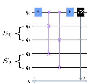
Figure S2: A schematic representation of a modified SWAP test employed to determine $\operatorname{Tr}(\hat{\rho}_{S_{1}}\hat{\rho}_{S_{2}})$ in a four-qubit system ($q=4$). Initially, qubits $q_{1}$ and $q_{2}$ are prepared in state $\hat{\rho}_{S_{1}}$, while qubits $q_{3}$ and $q_{4}$ are prepared in state $\hat{\rho}_{S_{2}}$. An ancilla qubit $q_{0}$ is introduced. The circuit involves a Hadamard gate applied to $q_{0}$, qubit-qubit controlled-SWAP gates between the two qubit sets, and a final Hadamard gate on $q_{0}$. By measuring $q_{0}$ multiple times and obtaining $P_{0}$, the quantity $\operatorname{Tr}(\hat{\rho}_{S_{1}}\hat{\rho}_{S_{2}})$ can be estimated as $2P_{0}-1$.

We are now prepared to demonstrate the validity of Eq. (S106). This proof will be conducted by constructing the proposed quantum circuit introduced in Ref. ekert_sm , illustrated in Fig. S2 for the specific scenario involving $q=4$ qubits and one ancilla qubit. Our system comprises an ancilla qubit $q_{0}$ and two subsystems, denoted as $S_{1}$ and $S_{2}$. Initially, the system’s density operator $\hat{\rho}$ is given by the tensor product:

$$\hat{\rho}=|0\rangle\langle 0|\otimes\hat{\rho}_{S_{1}}\otimes\hat{\rho}_{S_{2}}.$$ (S112)

Following the sequence of gates outlined in the quantum circuit, we define $\hat{\rho}^{(1)}=\hat{H}\hat{\rho}\hat{H}$, $\hat{\rho}^{(2)}=\bigl{(}\widehat{CSWAP}\bigr{)}\bigl{(}\hat{\rho}^{(1)}\bigr{)}\bigl{(}\widehat{CSWAP}\bigr{)}$ and $\hat{\rho}^{(3)}=\hat{H}\hat{\rho}^{(2)}\hat{H}$. Commencing with $\hat{\rho}^{(1)}$, we proceed by applying a Hadamard gate $\hat{H}$ to $q_{0}$:

$$\hat{\rho}^{(1)} =\hat{H}\hat{\rho}\hat{H}$$

$$=\frac{1}{2}(|0\rangle+|1\rangle)(\langle 0|+\langle 1|)\otimes\hat{\rho}_{S_{1}}\otimes\hat{\rho}_{S_{2}}$$

$$=|+\rangle\langle+|\otimes\hat{\rho}_{S_{1}}\otimes\hat{\rho}_{S_{2}},$$ (S113)

with $|+\rangle:=\frac{1}{\sqrt{2}}(|0\rangle+|1\rangle)$. By applying the controlled-SWAP gate $\widehat{CSWAP}$, we obtain

$$\hat{\rho}^{(2)} =\bigl{(}\widehat{CSWAP}\bigr{)}\bigl{(}\hat{\rho}^{(1)}\bigr{)}\bigl{(}\widehat{CSWAP}\bigr{)}$$

$$=\bigl{(}|0\rangle\langle 0|\otimes\hat{I}+|1\rangle\langle 1|\otimes\widehat{SWAP}\bigr{)}\bigl{(}|+\rangle\langle+|\otimes\hat{\rho}_{S_{1}}\otimes\hat{\rho}_{S_{2}}\bigr{)}\bigl{(}|0\rangle\langle 0|\otimes\hat{I}+|1\rangle\langle 1|\otimes\widehat{SWAP}\bigr{)}$$

$$=\frac{1}{\sqrt{2}}\bigl{(}|0\rangle\langle+|\otimes\hat{\rho}_{S_{1}}\otimes\hat{\rho}_{S_{2}}+|1\rangle\langle+|\otimes\widehat{SWAP}(\hat{\rho}_{S_{1}}\otimes\hat{\rho}_{S_{2}})\bigr{)}\bigl{(}|0\rangle\langle 0|\otimes\hat{I}+|1\rangle\langle 1|\otimes\widehat{SWAP}\bigr{)}$$

$$=\frac{1}{2}\bigl{(}|0\rangle\langle 0|\otimes\hat{\rho}_{S_{1}}\otimes\hat{\rho}_{S_{2}}+|1\rangle\langle 0|\otimes\widehat{SWAP}(\hat{\rho}_{S_{1}}\otimes\hat{\rho}_{S_{2}})+|0\rangle\langle 1|\otimes(\hat{\rho}_{S_{1}}\otimes\hat{\rho}_{S_{2}})\widehat{SWAP}$$

$$\quad+|1\rangle\langle 1|\otimes\widehat{SWAP}(\hat{\rho}_{S_{1}}\otimes\hat{\rho}_{S_{2}})\widehat{SWAP}\bigr{)}.$$ (S114)

To finalize, we apply another Hadamard gate to $q_{0}$:

$$\hat{\rho}^{(3)} =\hat{H}\hat{\rho}^{(2)}\hat{H}$$

$$=\frac{1}{2}\bigl{(}|+\rangle\langle+|\otimes\hat{\rho}_{S_{1}}\otimes\hat{\rho}_{S_{2}}+|-\rangle\langle+|\otimes\widehat{SWAP}(\hat{\rho}_{S_{1}}\otimes\hat{\rho}_{S_{2}})+|+\rangle\langle-|\otimes(\hat{\rho}_{S_{1}}\otimes\hat{\rho}_{S_{2}})\widehat{SWAP}$$

$$\quad+|-\rangle\langle-|\otimes\widehat{SWAP}(\hat{\rho}_{S_{1}}\otimes\hat{\rho}_{S_{2}})\widehat{SWAP}\bigr{)}.$$ (S115)

The next step is to calculate the reduced density operator $\hat{\rho}_{0}$ for the ancilla qubit. To do that, we take the partial trace over $S_{1}$ and $S_{2}$:

$$\hat{\rho}_{0} =\operatorname{Tr}_{S_{1}S_{2}}(\hat{\rho}^{(3)})$$

$$=\frac{1}{2}\bigl{(}|+\rangle\langle+|\operatorname{Tr}(\hat{\rho}_{S_{1}}\otimes\hat{\rho}_{S_{2}})+|-\rangle\langle+|\operatorname{Tr}(\widehat{SWAP}(\hat{\rho}_{S_{1}}\otimes\hat{\rho}_{S_{2}}))+|+\rangle\langle-|\operatorname{Tr}((\hat{\rho}_{S_{1}}\otimes\hat{\rho}_{S_{2}})\widehat{SWAP})$$

$$\quad+|-\rangle\langle-|\operatorname{Tr}(\widehat{SWAP}(\hat{\rho}_{S_{1}}\otimes\hat{\rho}_{S_{2}})\widehat{SWAP})\bigr{)}$$

$$=\frac{1}{2}\bigl{(}(|+\rangle\langle+|+|-\rangle\langle-|)+(|-\rangle\langle+|+|+\rangle\langle-|)\operatorname{Tr}((\hat{\rho}_{S_{1}}\otimes\hat{\rho}_{S_{2}})\widehat{SWAP})\bigr{)}$$

$$=\frac{\hat{I}+\operatorname{Tr}(\hat{\rho}_{S_{1}}\hat{\rho}_{S_{2}})\hat{Z}}{2},$$ (S116)

where in the last step we used the identity (S106). Thus, the probability $P_{0}=\operatorname{Tr}(|0\rangle\langle 0|\hat{\rho}_{0})$ of obtaining state $|0\rangle$ for the ancilla qubit is

$$P_{0} =\operatorname{Tr}\bigl{(}|0\rangle\langle 0|(\frac{\hat{I}+\operatorname{Tr}(\hat{\rho}_{S_{1}}\hat{\rho}_{S_{2}})\hat{Z}}{2})\bigr{)}$$

$$=\frac{1}{2}\operatorname{Tr}\bigl{(}|0\rangle\langle 0|+\operatorname{Tr}(\hat{\rho}_{S_{1}}\hat{\rho}_{S_{2}})|0\rangle\langle 0|\bigr{)}$$

$$=\frac{1+\operatorname{Tr}(\hat{\rho}_{S_{1}}\hat{\rho}_{S_{2}})}{2}.$$ (S117)

Therefore, we find that $\operatorname{Tr}(\hat{\rho}_{S_{1}}\hat{\rho}_{S_{2}})=2P_{0}-1.$ Now, specializing to the case where $\hat{\rho}_{S_{1}}=\hat{\rho}_{S_{2}}$, we obtain the purity:

$$\gamma_{S_{1}}=\operatorname{Tr}(\hat{\rho}^{2}_{S_{1}})=2P_{0}-1.$$ (S118)

In our quantum algorithm, $\gamma_{S_{1}}=\gamma_{A}$ is a function of time and is actually the reduced purity of subsystem $A$. The quantum circuit for this special case is shown in Fig. S3 for two identical systems $AB$ with $q=4$ qubits each.

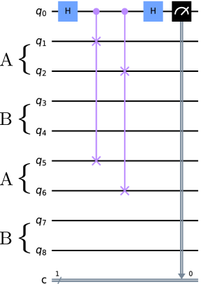
Figure S3: Quantum circuit used for the estimation of the reduced purity $\gamma_{A}$ of a system $AB$ composed by $q=4$ qubits. This circuit is analogous to the general case, with some exceptions. Here, the first $q$ qubits after the ancilla qubit $q_{0}$ and the last $q$ qubits are prepared in the same state $\hat{\rho}$. Also, the controlled-SWAP gates are applied only between the first half of qubits of each copy. Then, measuring $q_{0}$ for various identical circuits allows us to estimate the reduced purity $\gamma_{A}=\operatorname{Tr}(\hat{\rho}_{A}^{2})$, which corresponds to the bipartite reduced state of qubits $q_{1}$ and $q_{2}$ or $q_{5}$ and $q_{6}$.

References

• (1) D. M. Bressoud, Factorization and Primality Testing (Springer-Verlag, New York, 1989).
• (2) R. Crandall and C. Pomerance, Prime Numbers: A Computational Perspective (Springer, New York, 2005).
• (3) R. Baillie, A. Fiori, and S. S. Wagstaff Jr., Strengthening the Baillie-PSW primality test, Math. Comp. 90, 1931 (2021).
• (4) A. Granville, It is easy to determine whether a given integer is prime, Bull. Amer. Math. Soc. 42, 3 (2005).
• (5) D. Schumayer and D. A. W. Hutchinson, Colloquium: Physics of the Riemann hypothesis, Rev. Mod. Phys. 83, 307 (2011).
• (6) M. Wolf, Will a physicist prove the Riemann hypothesis?, Rep. Prog. Phys. 83, 036001 (2020).
• (7) C. Feiler and W. P. Schleich, Entanglement and analytical continuation: an intimate relation told by the Riemann zeta function, New J. Phys. 15, 063009 (2013).
• (8) G. Sierra and P. K. Townsend, Landau Levels and Riemann Zeros, Phys. Rev. Lett. 101, 110201 (2008).
• (9) S. Aaronson, The Prime Facts: From Euclid to AKS, https://www.scottaaronson.com/writings/prime.pdf (2003).
• (10) M. Agrawal, N. Kayal, and N. Saxena, PRIMES is in P, Annals of Mathematics 160, 781 (2004).
• (11) H. A. Helfgott, An improved sieve of Eratosthenes, Math. Comp. 89, 333 (2017).
• (12) G. L. Miller, Riemann’s Hypothesis and Tests for Primality, J. Comput. Syst. Sci. 13, 300 (1976).
• (13) L. M. Adleman, On Distinguishing Prime Numbers from Composite Numbers, Annals of Mathematics 117, 173 (1983).
• (14) A. Donis-Vela and J. C. Garcia-Escartin, A quantum primality test with order finding, Quantum Inf. Comp. 17, 1143 (2017).
• (15) H. F. Chau and H.-K. Lo, Primality Test Via Quantum Factorization, Int. J. Mod. Phys. C 08, 131 (1997).
• (16) J. Li, X. Peng, J. Du, and D. Suter, An Efficient Exact Quantum Algorithm for the Integer Square-free Decomposition Problem, Sci. Rep. 2, 1 (2012).
• (17) A. L. M. Southier, L. F. Santos, P. H. S. Ribeiro, and A. D. Ribeiro, Identifying primes from entanglement dynamics, Phys. Rev. A 108, 042404 (2023).
• (18) S. S. Bullock and I. L. Markov, Asymptotically optimal circuits for arbitrary n-qubit diagonal comutations, Quantum Info. Comput. 4, 27 (2004).
• (19) J. Welch, D. Greenbaum, S. Mostame, and A. Aspuru-Guzik, Efficient quantum circuits for diagonal unitaries without ancillas, New J. Phys. 16, 033040 (2014).
• (20) C. H. Bennett, H. J. Bernstein, S. Popescu, and B. Schumacher, Concentrating Partial Entanglement by Local Operations, Phys. Rev. A 53, 2046 (1996).
• (21) G. Vidal and R. Tarrach, Robustness of entanglement, Phys. Rev. A 59, 141 (1999).
• (22) M. L. W. Basso and J. Maziero, Entanglement monotones from complementarity relations, J. Phys. A: Math. Theor. 55, 355304 (2022).
• (23) A. K. Ekert, C. M. Alves, D. K. L. Oi, M. Horodecki, P. Horodecki, and L. C. Kwek, Direct Estimations of Linear and Nonlinear Functionals of a Quantum State, Phys. Rev. Lett. 88, 217901 (2002).
• (24) W. H. Press, S. A. Teukolsky, W. T. Vetterling, and B. P. Flannery, Numerical Recipes: The Art of Scientific Computing (Cambridge University Press, New York, 2007).
• (25) Qiskit contributors, Qiskit: An Open-source Framework for Quantum Computing, 2023, doi = 10.5281/zenodo.2573505.
• (26) M. A. Nielsen and I. L. Chuang, Quantum Computation and Quantum Information (Cambridge University Press, Cambridge, 2000).
• (27) J. Maziero, Computing partial traces and reduced density matrices, Int. J. Mod. Phys. C 28, 1750005 (2017).
• (28) G. B. Arfken, H. J. Weber, and F. E. Harris, Mathematical Methods for Physicists: A Comprehensive Guide, 7nd ed. (Elsevier, Oxford, 2013).
• (29) J. L. Walsh, A Closed Set of Normal Orthogonal Functions, Am. J. Math. 45, 5 (1923).
• (30) N. J. Fine, On the Walsh Functions, Trans. Am. Math. Soc. 65, 372 (1949).
• (31) L. Zhihua and Z. Qishan, Ordering of Walsh Functions, IEEE Trans. Electromagn. Compat. 25, 115 (1983).
• (32) C.-K. Yuen, Function Approximation by Walsh Series, IEEE Trans. Comp. 24, 590 (1975).
• (33) H. Buhrman, R. Cleve, J. Watrous, and R. de Wolf, Quantum Fingerprinting, Phys. Rev. Lett. 87, 167902 (2001).
• (34) A. Barenco, A. Berthiaume, D. Deutsch, A. Ekert, R. Jozsa, and C. Macchiavello, Stabilization of Quantum Computations by Symmetrization, SIAM J. Comput. 26, 1541 (1997).
• (35) S. Aaronson, Shadow tomography of quantum states, Proceedings of the 50th Annual ACM SIGACT Symposium on Theory of Computing, in STOC 2018. New York, NY, USA: Association for Computing Machinery, Jun. 2018, pp. 325–338. doi: 10.1145/3188745.3188802.
• (36) H.-Y. Huang, R. Kueng, and J. Preskill, Predicting many properties of a quantum system from very few measurements, Nat. Phys. 16, 10 (2020).
• (37) H. C. Nguyen, J. L. Bönsel, J. Steinberg, and O. Gühne, Optimising shadow tomography with generalised measurements, Phys. Rev. Lett. 129, 220502 (2022).
• (38) K. Bu, D. E. Koh, R. J. Garcia, and A. Jaffe, Classical shadows with Pauli-invariant unitary ensembles, npj Quantum Inf. 10, 1 (2024).
Supplemental Material: “Using quantum computers to identify prime numbers via entanglement dynamics” Victor F. dos Santos1,∗ and Jonas Maziero1,† 1Physics Department, Center for Natural and Exact Sciences, Federal University of
Santa Maria, Roraima Avenue 1000, 97105-900, Santa Maria, RS, Brazil

References

• (1) S. S. Bullock and I. L. Markov, Asymptotically optimal circuits for arbitrary n-qubit diagonal comutations, Quantum Info. Comput. 4, 27 (2004).
• (2) J. Welch, D. Greenbaum, S. Mostame, and A. Aspuru-Guzik, Efficient quantum circuits for diagonal unitaries without ancillas, New J. Phys. 16, 033040 (2014).
• (3) A. K. Ekert, C. M. Alves, D. K. L. Oi, M. Horodecki, P. Horodecki, and L. C. Kwek, Direct Estimations of Linear and Nonlinear Functionals of a Quantum State, Phys. Rev. Lett. 88, 217901 (2002).
• (4) J. L. Walsh, A Closed Set of Normal Orthogonal Functions, Am. J. Math. 45, 5 (1923).
• (5) N. J. Fine, On the Walsh Functions, Trans. Am. Math. Soc. 65, 372 (1949).
• (6) L. Zhihua and Z. Qishan, Ordering of Walsh Functions, IEEE Trans. Electromagn. Compat. 25, 115 (1983).
• (7) C. K. Yuen, Function Approximation by Walsh Series, IEEE Trans. Comp. 24, 590 (1975).
• (8) K. G. Beauchamp, Applications of Walsh and related functions, with an introduction to sequency theory, Vol. 2 (Academic press, 1984).
• (9) C. R. Edwards, The Application of the Rademacher–Walsh Transform to Boolean Function Classification and Threshold Logic Synthesis, in IEEE Trans. Comp. 24, 48 (1975).
• (10) M. A. Nielsen and I. L. Chuang, Quantum Computation and Quantum Information (Cambridge University Press, Cambridge, 2000).