AdaIR: Adaptive All-in-One Image Restoration via Frequency Mining and Modulation

Abstract

In the image acquisition process, various forms of degradation, including noise, blur, haze, and rain, are frequently introduced. These degradations typically arise from the inherent limitations of cameras or unfavorable ambient conditions. To recover clean images from their degraded versions, numerous specialized restoration methods have been developed, each targeting a specific type of degradation. Recently, all-in-one algorithms have garnered significant attention by addressing different types of degradations within a single model without requiring the prior information of the input degradation type. However, these methods purely operate in the spatial domain and do not delve into the distinct frequency variations inherent to different degradation types. To address this gap, we propose an adaptive all-in-one image restoration network based on frequency mining and modulation. Our approach is motivated by the observation that different degradation types impact the image content on different frequency subbands, thereby requiring different treatments for each restoration task. Specifically, we first mine low- and high-frequency information from the input features, guided by the adaptively decoupled spectra of the degraded image. The extracted features are then modulated by a bidirectional operator to facilitate interactions between different frequency components. Finally, the modulated features are merged into the original input for a progressively guided restoration. With this approach, the model achieves adaptive reconstruction by accentuating the informative frequency subbands according to different input degradations. Extensive experiments demonstrate that the proposed method, named AdaIR, achieves state-of-the-art performance on different image restoration tasks, including image denoising, dehazing, deraining, motion deblurring, and low-light image enhancement. Our code and pre-trained models are available at https://github.com/c-yn/AdaIRhttps://github.com/c-yn/AdaIR.

1 Introduction

Image restoration is the task of generating a high-quality clean image by removing degradations (e.g., noise, haze, blur, rain) from the original input image. It serves as a vital component in numerous downstream applications across diverse domains, including image/video content creation, surveillance, medical imaging, and remote sensing. Given its inherently ill-posed nature, effective image restoration demands learning strong image priors from large-scale data. To this end, deep neural network-based image restoration approaches [52, 18, 71, 49, 78, 59, 45, 80] have emerged as preferable choices over the conventional handcrafted algorithms [24, 37, 19, 57, 28, 42, 29]. Deep-learning methods learn image priors either implicitly from data [49, 78, 45, 80, 52, 18, 37], or explicitly by incorporating task-specific knowledge into the network architectures [60, 70, 62, 73, 72, 9]. Despite promising results on individual restoration tasks, these approaches are either not generalizable beyond the specific degradation types and levels which hinders their broader application, or require training separate copies of the same network on different degradation types, which is computationally expensive and tedious procedure, and maybe infeasible solution for deployment on resource-constraint edge-devices. Therefore, there is a need to develop an all-in-one image restoration method that can handle images with different degradation types, without requiring prior information regarding the corruption present in the input images.

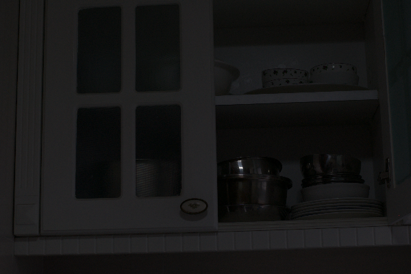
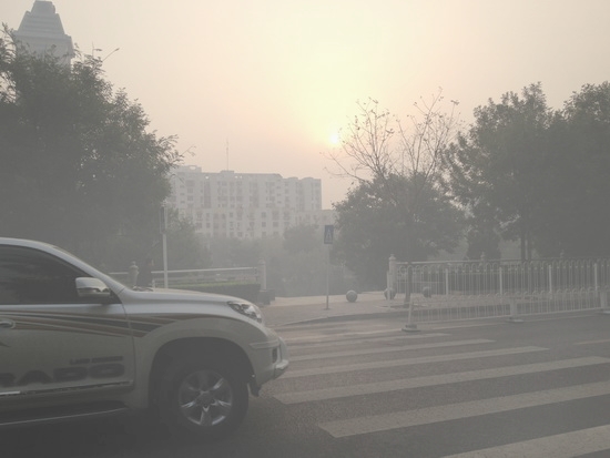
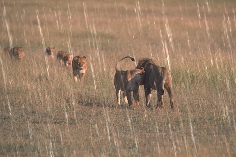
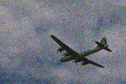
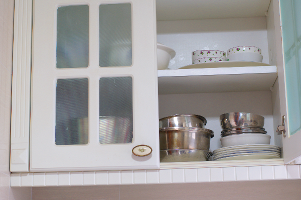
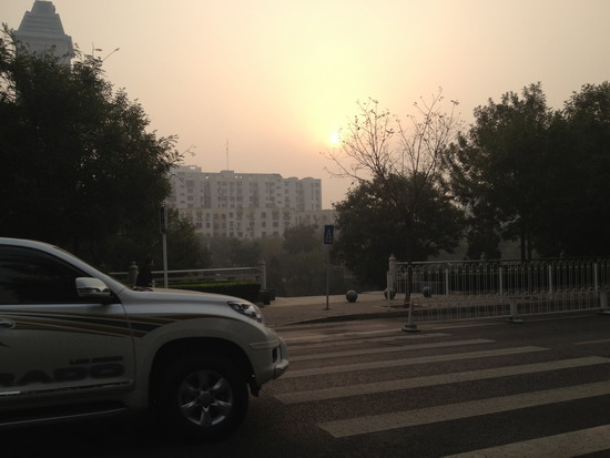
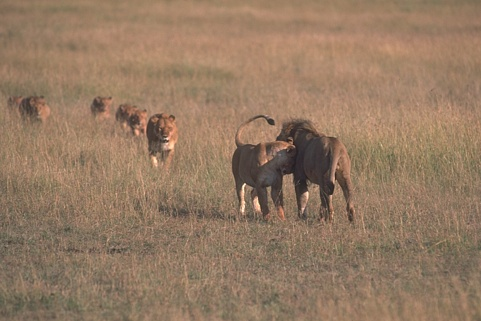
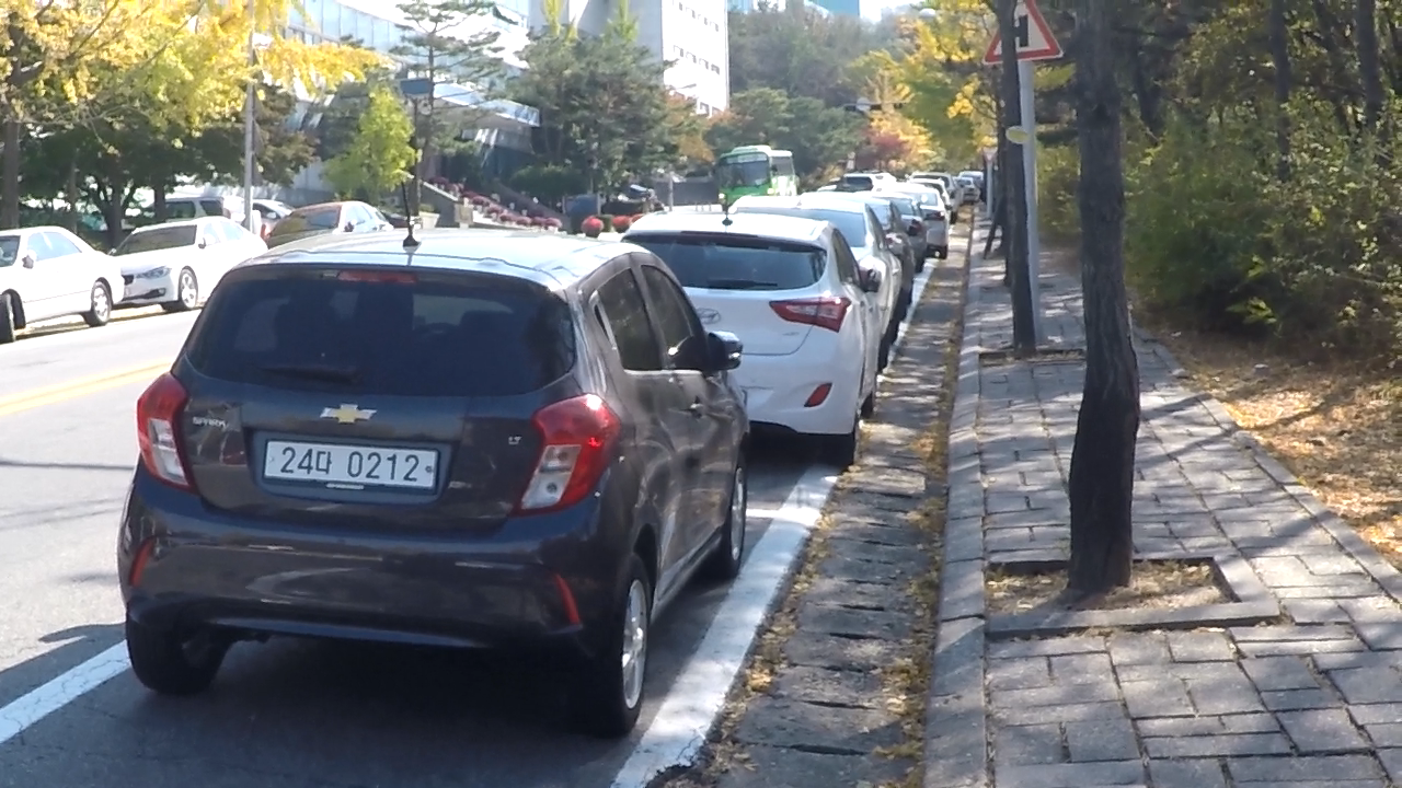
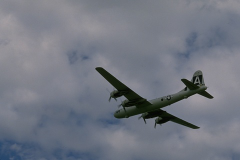
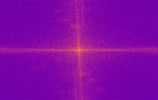
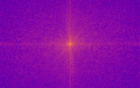
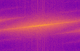
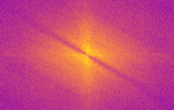
Low-Light	Dehazing	Deraining	Deblurring	Denoising

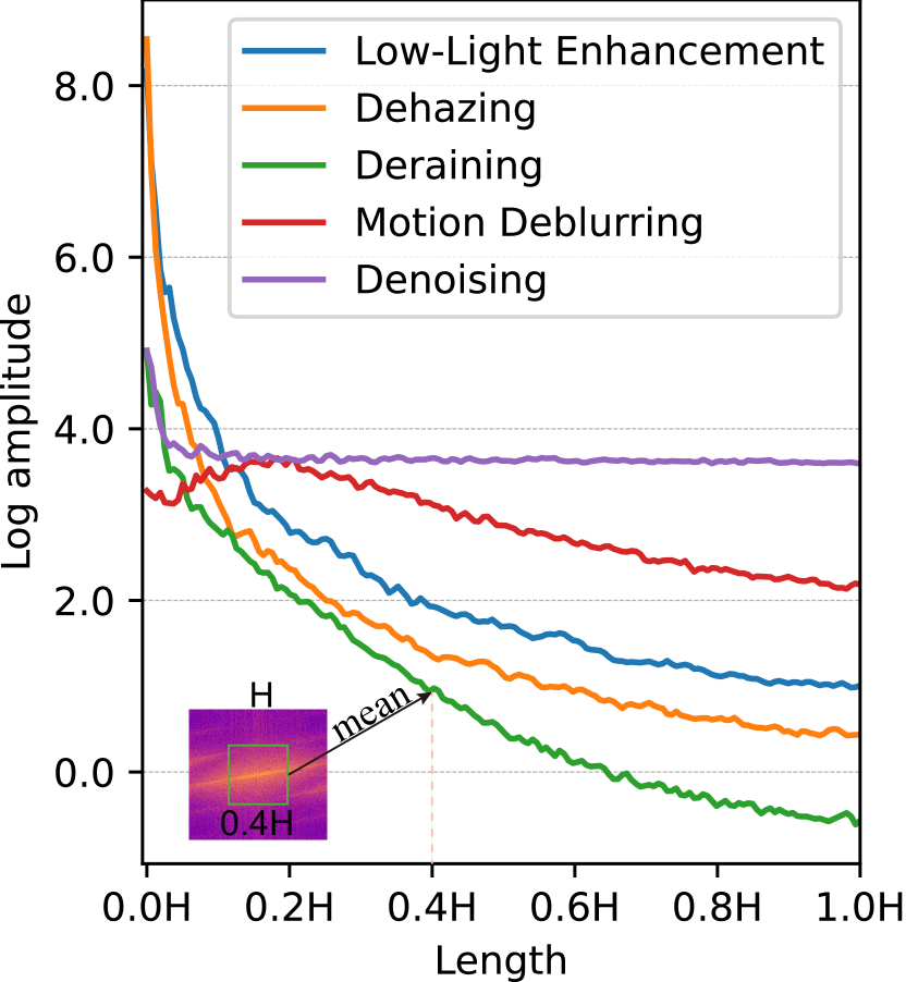
Figure 1: Left, from top to bottom: degraded images, ground-truth images, and the Fourier spectra of residual images obtained by subtracting the degraded images from the ground-truth images. The images are obtained from LOL-v1 [64], SOTS [32], Rain100L [32], GoPro [44], and BSD68 [41], respectively. Right, the sub-graph illustrates the mean values of Fourier spectra on the square of length shown on the x-axis, across five tasks. The spectra are all resized to $320\times 320$ for comparisons. As seen, different tasks pay different attention to different frequency subbands. For example, there are larger discrepancies in low frequency between degraded and target image pairs of the low-light image enhancement and dehazing datasets. In contrast, the frequency differences are generally evenly distributed for image denoising.

Recently, an increasing number of attempts have been made [33, 76, 46, 39] to address multiple degradations with a single model. These include employing a degradation-aware encoder in the restoration network learned via contrastive learning paradigm [33]; designing a two-stage framework IDR [76], where the first stage is dedicated to task-oriented knowledge collection based on underlying physics characteristics of degradation types, and the second stage is responsible for ingredients-oriented knowledge integration that progressively restores the image; or developing prompt-learning strategies [46, 39] inspired from their success in the natural language processing domain [5, 54, 30]. Nonetheless, all these approaches purely operate in the spatial domain, and do not consider frequency domain information. However, as illustrated in Fig. 1, we observe that different types of degradations may impact the image content on different frequency subbands. For instance, on the one hand, noisy and rainy images are contaminated with high-frequency content, while on the other hand, low-light and hazy images are dominated by low-frequency degraded content, thus indicating the need to treat each restoration task on its own merits.

In this paper, we propose an adaptive all-in-one image restoration framework based on frequency mining and modulation. Specifically, the frequency mining module extracts different frequency signals from the input features, guided by an adaptive spectra decomposition of the degraded input image. The extracted features are then refined using a bidirectional module, which facilitates the interactions between different frequency components by exchanging complementary information. Finally, these modulated features are used to transform the original input features via an efficient transposed cross-attention mechanism. With the proposed key design choices, our method can learn discriminative degradation context more effectively than other competing approaches, as shown in Fig. 2. Overall, the following are the main contributions of our work.

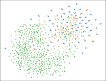
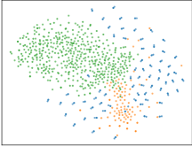
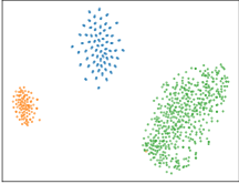
AirNet [33]	PromptIR [46]	Ours

Figure 2: The t-SNE results of intermediate features produced by the three-task all-in-one models. Our model is better at learning discriminative degradation contexts.

• We propose an adaptive all-in-one image restoration framework that leverages both spatial and frequency domain information to effectively decouple degradations from the desired clean image content.

• We introduce the Adaptive Frequency Learning Block (AFLB), which is a plugin block specifically designed for easy integration into existing image restoration architectures. The AFLB performs two sequential tasks: firstly, through its Frequency Mining Module (FMiM), it generates low- and high-frequency feature maps via guidance obtained from the spectra decomposition of the original degraded image; secondly, the Frequency Modulation Module (FMoM) within the AFLB calibrates these features by enabling the exchange of information across different frequency bands to effectively handle diverse types of image degradations.

• Extensive experiments demonstrate that our AdaIR algorithm sets new state-of-the-art performance on several all-in-one image restoration tasks, including image denoising, dehazing, deraining, motion deblurring, and low-light image enhancement.

2 Related Work

Single-Task Image Restoration. Image restoration is a fundamental task in computer vision that aims to reconstruct a clean image from its degraded counterpart. Since it is a highly ill-posed problem, many conventional methods have been proposed that utilize hand-crafted features and assumptions to reduce the solution space [4, 24]. Such solutions, though perform well on some datasets, may not generalize well to complicated real-world images [81]. Recently, with the rapid advancements in deep learning, a great number of convolutional neural network (CNN) based methods have been proposed and attained superior performance over traditional methods on various image restoration tasks, such as image denoising [77, 79], dehazing [47, 51], deraining [26, 50], and motion deblurring [13, 16]. To model long-range dependencies, Transformer models have been introduced to low-level tasks and significantly advanced state-of-the-art performance [23, 55, 58]. Despite the obtained promising performance, these task-specific methods lack generalization beyond certain degradation types and levels. For general image restoration, several network design-based approaches are proposed, which perform favorably on different restoration tasks  [62, 36, 35, 70]. Although these networks demonstrate robust performance on various restoration tasks, they require training separate copies on different datasets and tasks. Furthermore, applying a separate model for each possible degradation is resource-intensive, and often impractical for deployment, especially on edge devices.

All-in-One Image Restoration. All-in-one image restoration methods can address numerous degradations within a single model [46, 67, 27, 12]. Early unified models  [8, 34] employ distinct encoder and decoder heads to attend to different restoration tasks. However, these non-blind methods need prior knowledge about the degradation involved in the corrupted image in order to channelize it to the relevant restoration head. To achieve blind all-in-one image restoration, AirNet [33] learns the degradation representation from the corrupted images using the contrastive learning strategy, and the learned representation is then used to restore the clean image. The subsequent method, IDR [76], models different degradations depending on the underlying physics principles and achieves all-in-one image restoration in two stages. Recently, several prompt-learning-based schemes have been proposed [46, 39, 14, 1]. For instance, PromptIR [46] presets a series of tunable prompts to encode discriminative information about degradation types, which involve a large number of parameters. Different from the above-mentioned methods, which operate only in the spatial domain, this paper presents an all-in-one image restoration algorithm that exploits information both in spatial and frequency domains.

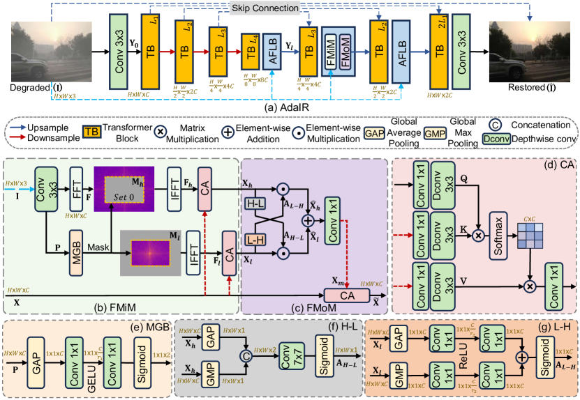
Figure 3: (a) The overall pipeline of the proposed AdaIR framework. It is a Transformer-based encoder-decoder architecture, employing novel Adaptive Frequency Learning Blocks (AFLB). Each AFLB contains (b) Frequency Mining Module (FMiM) that extracts different frequency components from input features guided by the adaptively decoupled spectra of the degraded input image, and (c) Frequency Modulation Module (FMoM) that exchanges the complementary information between different frequency features. (d) Cross Attention (CA). (e) Mask Generation Block (MGB) that yields a learnable frequency boundary for spectra decomposition. (f) H-L unit delivers high-frequency attention maps to enrich Low-frequency features. (g) L-H unit enhances high-frequency features by complementing it with low-frequency features. FFT and IFFT denote the Fast Fourier Transform and its inverse operator, respectively.

3 Method

Overall Pipeline. Figure 3 presents the pipeline of AdaIR. The overall goal of our AdaIR framework is to learn a unified model M that can recover a clean image $\hat{\textbf{I}}$ from a given degraded image I, without any prior information of degradation type D present in the input image I. Formally, given a degraded image I $\in\mathbb{R}^{H\times W\times 3}$, AdaIR first extracts shallow features $\mathbf{Y_{0}}$ $\in$ $\mathbb{R}^{H\times W\times C}$ using a ${3\times 3}$ convolution layer; where ${H\times W}$ denotes the spatial size and $C$ represents the number of channels. Next, these features $\mathbf{Y_{0}}$ are processed through a 4-level encoder-decoder network. Each level of the encoder employs multiple Transformer blocks (TBs) [70], where the number of blocks gradually increases from the top level to the bottom level, facilitating a computationally efficient design. The encoder takes high-resolution features $\mathbf{Y_{0}}$ as input, and progressively transforms them into a lower-resolution latent representation $\mathbf{Y}_{l}$ $\in$ $\mathbb{R}^{\frac{H}{8}\times\frac{W}{8}\times 8C}$. On the decoder side, the latent features $\mathbf{Y}_{l}$ are processed with interleaved Adaptive Frequency Learning Block (AFLB) and TBs to progressively reconstruct high-resolution clean output. Particularly, between every two levels of the decoder, we insert the AFLB that adaptively segregates the degradation content from the clean image content in the frequency domain, and subsequently assists in refining features in the spatial domain for effective image restoration.

Since different types of degradations affect image content at different frequency bands (as shown in Fig. 1), we specifically design the Adaptive Frequency Learning Block (AFLB) that extracts low- and high-frequency components from the input features and then modulate them to accentuate the corresponding informative subbands for each degradation. Next, we describe the two key components of AFLB: (1) Frequency Mining Module (FMiM) and Frequency Modulation Module (FMoM).

3.1 Frequency Mining Module (FMiM)

As shown in Fig. 3(b), given as inputs both the degraded image I and the intermediate features $\textbf{X}\in\mathbb{R}^{H\times W\times C}$, FMiM mines different frequency representations from X with the guidance of adaptively decoupled spectra of I. Primarily, FMiM consists of three steps, i.e., domain transformation, mask generation, and feature extraction.

For the domain transformation, FMiM applies a $3\times 3$ convolution layer on the degraded image I to expand the channel capacity to align with that of the input features X. These output features are then transformed into spectral domain representation $\textbf{F}\in\mathbb{R}^{H\times W\times C}$ via the Fast Fourier Transform (FFT).

Since we want to adaptively extract different frequency parts from the input features X, we design a lightweight Mask Generation Block (MGB) to generate a 2D mask that serves as a frequency boundary to separate the spectra of input image I. The cutoff frequency boundary adaptively changes according to the type of degradation present in the image. As illustrated in Fig. 3(e), the projected feature map P is first mapped into a vector using a global average pooling operator and then passes through two $1\times 1$ convolution layers with the GELU activation function in between to produce two factors ranging from 0 to 1, which define the mask size by multiplying with the width and height of the spectra. The mask generation process can be formally expressed as:

$$[\alpha,\beta]=\delta\left(W^{1\times 1}_{2}\left(\sigma\left(W^{1\times 1}_{1}\left(\textrm{GAP}_{\textrm{s}}\left(\textbf{P}\right)\right)\right)\right)\right)$$ (1)

where $\textrm{GAP}_{\textrm{s}}$ denotes spatial global average pooling, $\sigma$ represents the GELU activation function, and $\delta$ indicates the sigmoid function. The convolution weights ${W}_{1}$ and ${W}_{2}$ have the reduction ratios of $r_{1}$ and $\frac{C}{2r_{1}}$, respectively, progressively downsampling the channel dimensions to 2. Subsequently, the binary mask $\textbf{M}_{l}\in\{0,1\}^{H\times W}$ for extracting low frequency can be obtained by setting $\textbf{M}_{l}[\frac{H}{2}-\alpha\frac{H}{k}:\frac{H}{2}+\alpha\frac{H}{k},\frac{W}{2}-\beta\frac{W}{k}:\frac{W}{2}+\beta\frac{W}{k}]=1$, where $k$ is set to a small value of 128, as the curve junction is relatively small in Fig. 1. Accordingly, the mask for high frequency $\textbf{M}_{h}$ can be obtained by setting the values within the remaining region as 1. Subsequently, we can obtain the adaptively decoupled features by applying the learned masks to the spectra via element-wise multiplication and using the inverse Fourier transform.

Next, we adapt the multi-dconv head transposed cross attention (Fig. 3(d)) [70, 7] to mine the different feature parts from the input features with the guidance of $\textbf{F}_{l}$ and $\textbf{F}_{h}$. Overall, the feature extraction process is defined as:

$$\textbf{X}_{*}=\textrm{softmax}\left(\textbf{Q}\textbf{K}^{\top}/\alpha\right)\textbf{V},\quad\quad\textrm{where,}$$ (2)

$$\textbf{Q}={DW}_{1}\left({W}_{3}^{1\times 1}(\textbf{F}_{*})\right),\textbf{K}={DW}_{2}\left({W}_{4}^{1\times 1}(\textbf{X})\right),\textbf{V}={DW}_{3}\left({W}_{5}^{1\times 1}(\textbf{X})\right),\textrm{where,}$$ (3)

$$\textbf{F}_{*}=\mathcal{F}^{-1}\left(\textbf{M}_{*}\odot\textbf{F}\right),$$ (4)

where $*\in\{l,h\}$ is an indicator for low/high frequency, ${DW}$ represents a $3\times 3$ depth-wise convolution, $\odot$ is element-wise multiplication, $\mathcal{F}^{-1}$ indicates the inverse fast Fourier transform, Q, K and V are query, key and value projections, respectively, which are separately generated with a sequential application of ${1\times 1}$ convolution and $3\times 3$ depth-wise convolution, and $\alpha$ is a learnable scaling factor to control the magnitude of the dot product result of Q and K before using the softmax function.

3.2 Frequency Modulation Module (FMoM)

We devise FMoM to facilitate the cross interaction between the low-frequency mined features and high-frequency mined features, shown in Fig. 3(c). The goal is to cross complement one type of mined features with the other. For instance, high-frequency features contain edges and fine texture details, and thus we use this information to enrich low-frequency mined features via a super-lightweight spatial attention unit (H-L), depicted in Fig. 3(f). Similarly, the global information present in low-frequency features is passed to the high-frequency branch through the channel attention unit (L-H), illustrated in Fig. 3(g).

H-L Unit: This unit computes the spatial attention map from high-frequency mined features that are then used to complement features of the low-frequency branch. The H-L unit leverages two different channel-wise pooling techniques in parallel to produce two single-channel spatial feature maps, each of size $H\times W\times 1$. These maps are then concatenated along the channel dimension. The concatenated features are further refined with a $7\times 7$ convolution, followed by a sigmoid operation to generate the final spatial attention map, which is then used to obtain the modulated low-frequency features via element-wise multiplication. Overall, the process of the H-L Unit is given by:

$$\hat{\textbf{X}}_{l}=\textbf{X}_{l}\odot\textbf{A}_{H-L},\quad\quad\textrm{where,}$$ (5)

$$\textbf{A}_{H-L}=\delta\left(W^{7\times 7}_{6}([\textrm{GAP}_{c}(\textbf{X}_{h}),\textrm{GMP}_{c}(\textbf{X}_{h})])\right),$$ (6)

where $\textbf{W}_{6}$ has a channel reduction ratio of 2. $\delta$ is the sigmoid function. $\textrm{GAP}_{c}$ and $\textrm{GMP}_{c}$ are the channel-wise global average pooling and max pooling, respectively. $[\cdot,\cdot]$ indicates the concatenation operation.

L-H Unit: It is a dual branch module that processes incoming low-frequency mined features, yielding a feature descriptor that is subsequently used to attend to the high-frequency mined features. Specifically, given the mined low-frequency features $\textbf{X}_{l}\in\mathbb{R}^{H\times W\times C}$, the top branch of the L-H unit applies global average pooling along spatial dimension to obtain a feature vector of size $1\times 1\times C$, followed by two convolutional layers with the ReLU activation function in between. The bottom branch of the L-H unit employs the same structure, with the only difference of Max pooling at the head. The results of the two branches are added together, on which the sigmoid function is applied to produce the final attention descriptor $\textbf{A}_{L-H}\in\mathbb{R}^{1\times 1\times C}$, which is used to modulate the mined high-frequency features $\textbf{X}_{h}$. The process of the L-H Unit is expressed by:

$$\hat{\textbf{X}}_{h}=\textbf{X}_{h}\odot\textbf{A}_{L-H},\quad\quad\textrm{where,}$$ (7)

$$\textbf{A}_{L-H}=\delta\left(W_{8}^{1\times 1}\left(\gamma\left(W_{7}^{1\times 1}(\textrm{GAP}_{s}(\textbf{X}_{l})))\right)+W_{10}^{1\times 1}\left(\gamma(W_{9}^{1\times 1}(\textrm{GMP}_{s}(\textbf{X}_{l}))\right)\right)\right),$$ (8)

where $\delta$ is the sigmoid function, $\hat{\textbf{X}}_{h}$ is the modulated high-frequency features, $\textrm{GAP}_{s}$ and $\textrm{GMP}_{s}$ represent the global average pooling and max pooling along the spatial dimensions, respectively. $\gamma$ indicates the ReLU activation function. $\textbf{W}_{7}$ and $\textbf{W}_{9}$ have a reduction ratio of $r_{2}$ for the channel adjustment, while $\textbf{W}_{8}$ and $\textbf{W}_{10}$ have an increasing ratio of $r_{2}$. The parameters are shared among $\textbf{W}_{7}$ and $\textbf{W}_{9}$, $\textbf{W}_{8}$ and $\textbf{W}_{10}$ for computational efficiency.

Subsequently, the modulated high-frequency features $\hat{\textbf{X}}_{h}$ and low-frequency features $\hat{\textbf{X}}_{l}$ are aggregated and processed via a $1\times 1$ convolution to obtain $\textbf{X}_{m}$, which is merged into the original input features X using the cross-attention unit, where the query Q tensor is produced from X while $\textbf{X}_{m}$ yields the key K and value V tensors. By using FMiM and FMoM, the high-frequency and low-frequency contents of the input features are separately and adaptively modulated according to the degradation type present in the corrupted input image, leading to adaptive all-in-one image restoration.

4 Experiments

To validate the efficacy of the proposed AdaIR, we conduct experiments by strictly following previous state-of-the-art works [46, 33] under two different settings: (1) All-in-One, and (2) Single-task. In the All-in-One setting, a unified model is trained to perform image restoration across multiple degradation types. Whereas, within the Single-task setting, separate models are trained for each specific restoration task. We provide additional ablation experiments, visual examples, and more details on the architecture in the supplementary material. In tables, the best and second-best image fidelity scores (PSNR and SSIM [63]) are highlighted in red and blue, respectively.

Implementation Details. Our AdaIR presents an end-to-end trainable solution without the necessity for pretraining any individual component. The architecture of AdaIR employs a 4-level encoder-decoder structure, with varying numbers of Transformer blocks (TB) at each level, specifically [4, 6, 6, 8] from level-1 to level-4. We integrate one AFLB block between every two consecutive decoder levels, amounting to a total of three AFLBs in the overall network.

For training, we adopt a batch size of 32 in the all-in-one setting, and a batch size of 8 in the single-task setting. The network optimization is achieved through an L1 loss function, employing the Adam optimizer ($\beta 1=0.9$ and $\beta 2=0.999$), with a learning rate of $2e^{-4}$, over the course of 150 epochs. During the training process, cropped patches sized at ${128\times 128}$ pixels are provided as input, with additional augmentation applied via random horizontal and vertical flips.

Datasets. In preparing datasets for training and testing, we closely follow prior works [46, 33]. For single-task image dehazing, we use SOTS [32] dataset that comprises 72,135 training images and 500 testing images. For single-task image deraining, we utilize the Rain100L [68] dataset, which contains 200 clean-rainy image pairs for training and 100 pairs for testing. For single-task image denoising, we combine images of BSD400 [2] and WED [40] datasets for model training; the BSD400 encompasses 400 training images, while the WED dataset consists of 4,744 images. Starting from these clean images of BSD400 [2] and WED [40], we generate their corresponding noisy versions by adding Gaussian noise with varying levels ($\sigma\in\{15,25,50\}$). Denoising task evaluation is performed on the BSD68 [41] and Urban100 [25] datasets. Finally, under the all-in-one setting, we train a single model on the combined set of the aforementioned training datasets, and directly test it across multiple restoration tasks.

Table 1: Comparisons under the three-degradation all-in-one setting: a unified model is trained on a combined set of images obtained from all degradation types and levels. On Rain100L [68] for image deraining, AdaIR yields 2.27 dB gain over PromptIR [46].

	Dehazing	Deraining	Denoising on BSD68 [41]
Method	on SOTS [32]	on Rain100L [68]	$\sigma=15$	$\sigma=25$	$\sigma=50$	Average
BRDNet [56]	23.23/0.895	27.42/0.895	32.26/0.898	29.76/0.836	26.34/0.693	27.80/0.843
LPNet [22]	20.84/0.828	24.88/0.784	26.47/0.778	24.77/0.748	21.26/0.552	23.64/0.738
FDGAN [20]	24.71/0.929	29.89/0.933	30.25/0.910	28.81/0.868	26.43/0.776	28.02/0.883
MPRNet  [73]	25.28/0.955	33.57/0.954	33.54/0.927	30.89/0.880	27.56/0.779	30.17/0.899
DL [21]	26.92/0.931	32.62/0.931	33.05/0.914	30.41/0.861	26.90/0.740	29.98/0.876
AirNet [33]	27.94/0.962	34.90/0.968	33.92/0.933	31.26/0.888	28.00/0.797	31.20/0.910
PromptIR [46]	30.58/0.974	36.37/0.972	33.98/0.933	31.31/0.888	28.06/0.799	32.06/0.913
AdaIR (Ours)	31.06/0.980	38.64/0.983	34.12/0.935	31.45/0.892	28.19/0.802	32.69/0.918

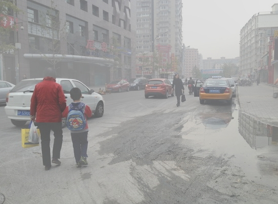
Degraded	7.84 dB	23.09 dB	25.30 dB	30.80 dB	PSNR
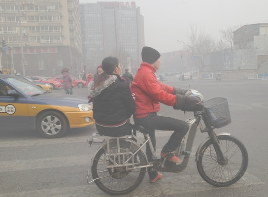
Degraded	10.82 dB	27.49 dB	28.75 dB	31.68 dB	PSNR
Degraded	9.57 dB	19.34 dB	19.88 dB	24.61 dB	PSNR
Image	Input	AirNet	PromptIR	AdaIR	Reference

Figure 4: Image dehazing comparisons on SOTS [32] between all-in-one methods. Compared to other algorithms, our method is more effective in haze removal.

Degraded	16.92 dB	28.40 dB	28.81 dB	31.38 dB	PSNR
Degraded	23.16 dB	31.12 dB	33.64 dB	38.66 dB	PSNR
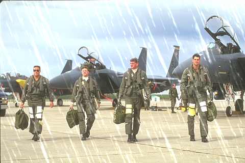
Degraded	27.49 dB	35.53 dB	39.25 dB	44.90 dB	PSNR
Image	Input	AirNet	PromptIR	AdaIR	Reference

Figure 5: Image deraining results on Rain100L [68] between all-in-one methods. AdaIR yields high-fidelity rain-free images with structural fidelity and without streak artifacts.

4.1 All-in-One Results: Three Distinct Degradations

We evaluate the performance of our all-in-one AdaIR model on three different restoration tasks, including image dehazing, deraining, and denoising. We compare AdaIR against various general image restoration methods (BRDNet [56], LPNet [22], FDGAN [20], and MPRNet [73]), as well as specialized all-in-one approaches (DL [21], AirNet [33], and PromptIR [46]). Table 1 shows that the proposed AdaIR provides consistent performance gains over the other competing approaches. When averaged across various restoration tasks and settings, our AdaIR obtains $0.63$ dB PSNR gain over the recent best method PromptIR [46], and $1.49$ dB improvement over the second best algorithm AirNet [33]. Specifically, compared to PromptIR [46], AdaIR yields a substantial boost of $2.27$ dB on the deraining task, and $0.48$ dB on the dehazing task. We provide visual examples in Fig. 4 for dehazing, Fig. 5 for deraining, and Fig. 6 for denoising. These examples show that our AdaIR is effective in removing degradations, and generates images that are visually closer to the ground truth than those of the other approaches [46, 33]. Particularly, in the restored images, our method preserves better structural fidelity and fine textures.

4.2 Single Degradation One-by-One Results

Consistent with previous works [33, 46], we further evaluate AdaIR under the single-task experimental protocol. To this end, we train separate copies of AdaIR model for each distinct restoration task. Table 2 reports dehazing results; compared to the previous all-in-one approaches PromptIR [46] and AirNet [33], our method obtains PSNR gains of $0.49$ dB and $8.62$ dB, respectively. Similarly, on the deraining task, our AdaIR advances the state-of-the-art [46] by $1.86$ dB as shown in Table 3. A similar performance trend can be observed in image quality scores provided in Table 4 for denoising.

Degraded	14.95 dB	33.11 dB	32.91 dB	34.02 dB	PSNR
Degraded	14.89 dB	27.19 dB	27.23 dB	27.68 dB	PSNR
Degraded	15.63 dB	26.73 dB	26.18 dB	27.12 dB	PSNR
Image	Input	AirNet	PromptIR	AdaIR	Reference

Figure 6: Image denoising comparisons on BSD68 [41] between all-in-one methods. The image reproduction quality of our AdaIR is more visually faithful to the ground truth.

Table 2: Dehazing results in the single-task setting on the SOTS-Outdoor [32] dataset. Compared to PromptIR [46], our method generates a 0.49 dB PSNR improvement.

	DehazeNet	MSCNN	AODNet	EPDN	FDGAN	AirNet	Restormer	PromptIR	AdaIR
Method	[6]	[51]	[31]	[48]	[20]	[33]	[70]	[46]	(Ours)
PSNR	22.46	22.06	20.29	22.57	23.15	23.18	30.87	31.31	31.80
SSIM	0.851	0.908	0.877	0.863	0.921	0.900	0.969	0.973	0.981

Table 3: Deraining results in the single-task setting on the Rain100L [68] dataset. Our AdaIR obtains a significant performance boost of 1.86 dB PSNR over PromptIR [46].

	DIDMDN	UMR	SIRR	MSPFN	LPNet	AirNet	Restormer	PromptIR	AdaIR
Method	[75]	[69]	[65]	[26]	[22]	[33]	[70]	[46]	(Ours)
PSNR	23.79	32.39	32.37	33.50	33.61	34.90	36.74	37.04	38.90
SSIM	0.773	0.921	0.926	0.948	0.958	0.977	0.978	0.979	0.985

Table 4: Denoising results in the single-task setting on Urban100 [25] and BSD68 [41]. On Urban100 [25] for the noise level 50, AdaIR yields a 0.31 dB gain over PromptIR [46].

	Urban100			BSD68
Method	$\sigma=15$	$\sigma=25$	$\sigma=50$	$\sigma=15$	$\sigma=25$	$\sigma=50$	Average
CBM3D [17]	33.93/0.941	31.36/0.909	27.93/0.840	33.50/0.922	30.69/0.868	27.36/0.763	30.80/0.874
DnCNN [77]	32.98/0.931	30.81/0.902	27.59/0.833	33.89/0.930	31.23/0.883	27.92/0.789	30.74/0.878
IRCNN [78]	27.59/0.833	31.20/0.909	27.70/0.840	33.87/0.929	31.18/0.882	27.88/0.790	29.90/0.864
FFDNet [79]	33.83/0.942	31.40/0.912	28.05/0.848	33.87/0.929	31.21/0.882	27.96/0.789	31.05/0.884
BRDNet [56]	34.42/0.946	31.99/0.919	28.56/0.858	34.10/0.929	31.43/0.885	28.16/0.794	31.44/0.889
AirNet [33]	34.40/0.949	32.10/0.924	28.88/0.871	34.14/0.936	31.48/0.893	28.23/0.806	31.54/0.897
PromptIR [46]	34.77/0.952	32.49/0.929	29.39/0.881	34.34/0.938	31.71/0.897	28.49/0.813	31.87/0.902
AdaIR (Ours)	34.96/0.953	32.74/0.931	29.70/0.885	34.36/0.938	31.72/0.897	28.49/0.813	32.00/0.903

Table 5: Comparisons for five-degradation all-in-one restoration. Denoising results are reported for the noise level $\sigma=25$. The top super-row methods denote the general image restoration approaches, and the rest are specialized all-in-one approaches. On SOTS [68] for dehazing, AdaIR attains a remarkable gain of 5.29 dB over IDR [76].

	Dehazing	Deraining	Denoising	Deblurring	Low-Light
Method	on SOTS	on Rain100L	on BSD68	on GoPro	on LOL	Average
NAFNet [9]	25.23/0.939	35.56/0.967	31.02/0.883	26.53/0.808	20.49/0.809	27.76/0.881
HINet [10]	24.74/0.937	35.67/0.969	31.00/0.881	26.12/0.788	19.47/0.800	27.40/0.875
MPRNet [73]	24.27/0.937	38.16/0.981	31.35/0.889	26.87/0.823	20.84/0.824	28.27/0.890
DGUNet [43]	24.78/0.940	36.62/0.971	31.10/0.883	27.25/0.837	21.87/0.823	28.32/0.891
MIRNetV2 [74]	24.03/0.927	33.89/0.954	30.97/0.881	26.30/0.799	21.52/0.815	27.34/0.875
SwinIR [36]	21.50/0.891	30.78/0.923	30.59/0.868	24.52/0.773	17.81/0.723	25.04/0.835
Restormer [70]	24.09/0.927	34.81/0.962	31.49/0.884	27.22/0.829	20.41/0.806	27.60/0.881
DL [21]	20.54/0.826	21.96/0.762	23.09/0.745	19.86/0.672	19.83/0.712	21.05/0.743
Transweather [61]	21.32/0.885	29.43/0.905	29.00/0.841	25.12/0.757	21.21/0.792	25.22/0.836
TAPE [38]	22.16/0.861	29.67/0.904	30.18/0.855	24.47/0.763	18.97/0.621	25.09/0.801
AirNet [33]	21.04/0.884	32.98/0.951	30.91/0.882	24.35/0.781	18.18/0.735	25.49/0.846
IDR [76]	25.24/0.943	35.63/0.965	31.60/0.887	27.87/0.846	21.34/0.826	28.34/0.893
AdaIR (Ours)	30.53/0.978	38.02/0.981	31.35/0.889	28.12/0.858	23.00/0.845	30.20/0.910

Table 6: Image denoising results of directly applying the pre-trained model under the five-degradation setting to the Urban100 [25], Kodak24 [53] and BSD68 [41] datasets. The results are PSNR scores. On Urban100 [25] for the noise level $\sigma=25$, AdaIR produces a significant performance gain of 0.39 dB PSNR over IDR [76].

	Urban100			Kodak24			BSD68
Method	$\sigma=15$	$\sigma=25$	$\sigma=50$	$\sigma=15$	$\sigma=25$	$\sigma=50$	$\sigma=15$	$\sigma=25$	$\sigma=50$	Average
DL [21]	21.10	21.28	20.42	22.63	22.66	21.95	23.16	23.09	22.09	22.04
Transweather [61]	29.64	27.97	26.08	31.67	29.64	26.74	31.16	29.00	26.08	28.66
TAPE [38]	32.19	29.65	25.87	33.24	30.70	27.19	32.86	30.18	26.63	29.83
AirNet [33]	33.16	30.83	27.45	34.14	31.74	28.59	33.49	30.91	27.66	30.89
IDR [76]	33.82	31.29	28.07	34.78	32.42	29.13	34.11	31.60	28.14	31.48
AdaIR (Ours)	34.10	31.68	28.29	34.89	32.38	29.21	34.01	31.35	28.06	31.55

4.3 Additional All-in-One Results: Five Distinct Degradations

Following the recent work of IDR [76], we further verify the effectiveness of AdaIR by performing experiments on five restoration tasks: dehazing, deraining, denoising, deblurring, and low-light image enhancement. For this, we train an all-in-one AdaIR model on combined datasets gathered for five different tasks. These include datasets from the aforementioned three-task setting as well as additional datasets: GoPro [44] for motion deblurring, and LOL-v1 [64] for low-light image enhancement.

Table 5 shows that AdaIR achieves a $1.86$ dB gain compared to the recent best method IDR [76], when averaged across five restoration tasks. Particularly, the performance improvement is over $5$ dB on dehazing. Table 6 reports denoising results on three different datasets with various noise levels. It can be seen that our method performs favorably well compared to the other competing approaches.

Table 7: Ablation studies for the proposed components. Fixed uses a fixed square mask with sides of 10. FLOPs are measured on the patch size of $256\times 256\times 3$.

		FMiM		FMoM				Overhead
Net	Baseline	Fixed	MGB	L-H	H-L	PSNR	SSIM	Params.	FLOPs
(a)	✓					28.21	0.966	26.13M	141.24G
(b)	✓	✓				29.79	0.969	27.73M	145.09G
(c)	✓	✓		✓		30.37	0.975	28.74M	147.44G
(d)	✓	✓		✓	✓	30.52	0.976	28.74M	147.44G
(e)	✓		✓	✓	✓	31.24	0.978	28.77M	147.45G

4.4 Ablation Studies

In this section, we conduct ablation studies to test the impact of various individual components to the overall performance of AdaIR. All ablation experiments are performed on the image dehazing task by training models for 20 epochs.

Impact of individual architecture modules. Table 7 summarizes the performance benefits of individual architectural contributions. Table 7(b) demonstrates that the proposed frequency mining mechanism (FMiM) brings gains of $1.58$ dB PSNR over the baseline model, using only a fixed mask to decompose the spectra of input images. Furthermore, the L-H unit boosts the performance to $30.37$ dB PSNR; see Table 7(c). It can be seen in Table 7(d) that we use both L-H and H-L units, and the performance reaches $30.52$ dB PSNR. Finally, Table 7(e) shows that the overall AdaIR brings $3.03$ dB improvement over the baseline, while incurring a small computational overhead of 2.64M parameters and 6.21 GFlops. These results corroborate the effectiveness of our design.

Strategies for spectral decomposition. We carry out this ablation to test different strategies to segregate low- and high-frequency representations from the degraded input images. We compare the proposed mask-guided adaptive frequency decomposition approach with the Average pooling and Gaussian filtering strategies. Results are provided in Table 9. Following  [15], we use average pooling to obtain the low-frequency features which are then subtracted from the input features to obtain the high-frequency features. This strategy provides PSNR of $30.59$ (see column 1 in Table 9), which is $0.65$ dB lower than our method. Similarly, when we switch to the Gaussian filter of size ${5\times 5}$, the model achieves only $30.22$ dB PSNR (second column). In contrast, our method of applying a flexible mask for Fourier spectra decomposition performs the best, yielding $31.24$ dB.

Table 8: Spectra decomposition methods.

Methods	Average Pooling	Gaussian Filter	Ours
PSNR	30.59	30.22	31.24
SSIM	0.976	0.976	0.978

Table 9: Degradation sources.

Method	Embedding	Ours
PSNR	29.29	30.52
SSIM	0.969	0.976

Table 10: Results on the unseen desnowing task with the CSD [11] dataset.

Method	AirNet [33]	PromptIR [46]	Ours
PSNR	19.32	20.47	20.54
SSIM	0.733	0.7638	0.7643

Table 11: Results on mixed degradations, Rain100L with the Gaussian noise $\sigma=50$.

Method	AirNet [33]	PromptIR [46]	Ours
PSNR	27.25	27.34	27.51
SSIM	0.790	0.791	0.799

Frequency representation mining at image-level vs. feature-level. Each AFLB block in AdaIR decoder receives the original degraded image as input, on which FMiM applies the procedure of spectra decomposition. To verify the efficacy of this design, we switch to using the input embedding features $\mathbf{X}$ (rather than degraded image) for frequency representation. This ablation result in Table 9 shows a performance drop from $30.52$ dB to $29.29$ dB, indicating that the raw input image offers better discriminative information about the degradation for effective spectra separation.

Generalization to out-of-distribution degradations. To show the generalization ability of our AdaIR, we take the all-in-one model trained on the three-task setting, and directly test it under two different scenarios: (1) unseen degradation type, and (2) multi-degraded images. Table 11 shows that, on the unseen task of image desnowing, AdaIR provides more favorable results than other approaches. We create a mixed degradation dataset by adding Gaussian noise (level $\sigma=50$) to the rainy images of Rain100L [68]. Table 11 depicts that our method is more robust in the mixed degradation scenes than PromptIR [46] and AirNet [33].

5 Conclusion

This paper introduces AdaIR, an all-in-one image restoration model capable of adaptively removing different kinds of image degradations. Motivated by the observation that different degradations affect distinct frequency bands, we have developed two novel components: a frequency mining module and a frequency modulation module. These modules are designed to identify and enhance the relevant frequency components based on the degradation patterns present in the input image. Specifically, the frequency mining module extracts specific frequency elements from the image’s intermediate features, guided by an adaptive decomposition of the input’s spectral characteristics that reflect the underlying degradation. Subsequently, the frequency modulation module further refines these elements by facilitating the exchange of complementary information across different frequency features. Incorporating the proposed modules into a U-shaped Transformer backbone, the proposed network achieves state-of-the-art performance on a range of image restoration tasks.

This supplementary material provides additional ablation studies (Sec. 0.A), computational comparisons (Sec. 0.B), architectural details of the transformer block (Sec. 0.C), and additional visual results (Sec. 0.D).

Appendix 0.A Additional Ablation Studies

AFLBs in encoder and decoder? We run an experiment to assess the feasibility of employing AFLB modules on either the encoder side, decoder side, or both. Table 12 shows that utilizing AFLBs in both the encoder and decoder leads to notable performance degradation compared to AFLBs solely integrated into the decoder.

Table 12: Comparisons of image dehazing under the single-task setting: between the use of AFLBs on either the encoder-side, decoder-side, or both.

	Dehazing on SOTS [32]
Method	PSNR	SSIM
Encoder+Decoder+AFLB	29.70	0.973
AdaIR (Ours)	30.52	0.976

Placement of AFLB in the network. Next, we conduct an ablation experiment to study where to place AFLBs in our hierarchical network. Table 13 demonstrates that employing only one AFLB (between level 1 and level 2) leads to a deterioration in the network’s performance (29.58 dB in top row). Conversely, integrating AFLBs between every consecutive level of the decoder yields the best performance.

Table 13: AFLB position. Results are reported on the SOTS [32] dataset.

Method	PSNR	SSIM
Level 2	28.58	0.973
Level 2+3	29.83	0.975
Level 2+3+4	30.52	0.976

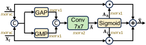
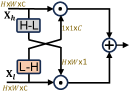
(a) Spatial attention, 29.67 dB/0.973	(b) Ours, 30.52 dB/0.976

Figure 7: Different choices for FMoM. (a) Using widely adopted spatial attention [66] to modulate different frequency features, where the attention map is generated without discriminating different frequency inputs. (b) Using specially designed attention units to exchange complementary information across different frequency features. GAP and GMP denote the global average pooling and global max pooling, respectively. The experiments are conducted on image dehazing under the single-task setting.

Design choices of FMoM. We investigate different choices for the frequency modulation module (FMoM). As shown in Fig. 7(a), we leverage the commonly used spatial attention [66] to modulate different frequency features without discriminating different inputs. Overall, the process is formally given by:

$$\hat{\textbf{X}}=\textbf{X}_{h}\odot\textbf{A}_{h}+\textbf{X}_{l}\odot\textbf{A}_{l},\quad\quad\textrm{where},$$ (9)

$$\textbf{A}_{h},\textbf{A}_{l}=\textrm{Split}\left(\delta(\widetilde{\textbf{A}})\right),\quad\quad\textrm{where},$$ (10)

$$\widetilde{\textbf{A}}=W^{7\times 7}\left([\textrm{GAP}([\textbf{X}_{h},\textbf{X}_{l}]),\textrm{GMP}([\textbf{X}_{h},\textbf{X}_{l}])]\right)$$ (11)

where $\odot$ represents element-wise multiplication, Split indicates splitting the features among the channel dimension, $\delta$ is the Sigmoid function, $W^{7\times 7}$ is a $7\times 7$ convolution, and $[\cdot,\cdot]$ is a concatenation operator. GAP and GMP are global average pooling and global max pooling among the channel dimensions, respectively. The experiments are performed on the image dehazing task under the single-task setting. This variant achieves only 29.67 dB PSNR, which is 0.85 dB lower than our FMoM, shown in Fig. 7(b), indicating the effectiveness of our design.

Combinations of different degradations. We investigate the influence of various combinations of degradation types on model performance, as presented in Table 14. As expected, including more degradation types make it increasingly difficult for the model to perform restoration. Notable, hazy images in a combined dataset lead to a larger performance drop than rainy or noisy images. One reason could be that the aim of the restoration model in deraining and denoising tasks is to focus more on restoring high-frequency content (noise, rain), whereas, in the dehazing task the goal is to focus on removing low-frequency (hazy) content.

Table 14: Ablation studies on the combinations of degradations for the three-task setting. Results are presented in the form of PSNR (dB)/SSIM.

Degradation			Denoising on BSD68			Deraining on	Dehazing
Noise	Rain	Haze	$\sigma=15$	$\sigma=25$	$\sigma=50$	on Rain100L	on SOTS
✓			34.36/0.938	31.72/0.897	28.49/0.813	-	-
	✓		-	-	-	38.90/0.985	-
		✓	-	-	-	-	31.80/0.981
✓	✓		34.31/0.938	31.67/0.896	28.42/0.811	38.22/0.983	-
✓		✓	34.11/0.935	31.48/0.892	28.19/0.802	-	30.89/0.980
	✓	✓	-	-	-	38.44/0.983	30.54/0.978
✓	✓	✓	34.12/0.935	31.45/0.892	28.19/0.802	38.64/0.983	31.06/0.980

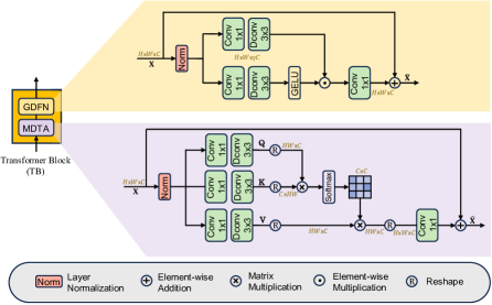
Figure 8: Architectural details of the Transformer Block (TB) used in the AdaIR framework. TB involves two elements: multi-dconv head transposed attention (MDTA) and gated-dconv feed-forward network (GDFN).

Appendix 0.B Computational Comparisons

Table 15 shows that the proposed AdaIR strikes a better tradeoff between accuracy and complexity than other all-in-one competing methods.

Table 15: Computational comparisons of all-in-one methods under the three-degradation setting. Average PSNR across three tasks is reported here (see Table 1 of the main paper for more detailed results). FLOPs are measured on the patch size of $256\times 256\times 3$.

	Params.	FLOPs	PSNR
Method	(M)	(G)
AirNet [33]	8.93	311	31.20
PromptIR [46]	35.59	158.4	32.06
AdaIR	28.77	147.45	32.69

Appendix 0.C Transformer Block in the AdaIR Framework

In the AdaIR framework, we use Transformer Blocks (TB) based on the design proposed in [70]. Fig. 8 presents its architectural details. It consists of two successive components, multi-dconv head transposed attention (MDTA) and gated-dconv feed-forward network (GDFN).

MDTA first normalizes the input $\textbf{X}\in\mathbb{R}^{H\times W\times C}$ using a layer normalization operator [3], and then generates the query (Q$\in\mathbb{R}^{H\times W\times C}$), key (K$\in\mathbb{R}^{H\times W\times C}$), and value (V$\in\mathbb{R}^{H\times W\times C}$) projections using combinations of $1\times 1$ convolution and $3\times 3$ depth-wise convolution layers. The transposed-attention map of size $C\times C$ is yielded by applying the Softmax function to the dot-product results of the reshaped query and key projections. Overall, the process of MDTA is given by:

$$\hat{\textbf{X}}=W^{1\times 1}_{1}\textrm{Attention}\left(\textbf{Q}^{\prime},\textbf{K}^{\prime},\textbf{V}^{\prime}\right)+\textbf{X},\quad\quad\textrm{where,}$$ (12)

$$\textrm{Attention}\left(\textbf{Q}^{\prime},\textbf{K}^{\prime},\textbf{V}^{\prime}\right)=\textbf{V}^{\prime}\cdot\textrm{Softmax}\left(\textbf{K}^{\prime}\cdot\textbf{Q}^{\prime}/\alpha\right),$$ (13)

where $\hat{\textbf{X}}$ is the output of MDTA. $W_{1}^{1\times 1}$ denotes a $1\times 1$ convolution. $\alpha$ is a learnable factor to control the magnitude of the dot product result of K and Q. $\textbf{Q}^{\prime}$, $\textbf{K}^{\prime}$ and $\textbf{V}^{\prime}$ are obtained by reshaping tensors from the original size $\mathbb{R}^{H\times W\times C}$.

Similarly, GDFN first applies a layer normalization operator to normalize the input $\textbf{X}\in\mathbb{R}^{H\times W\times C}$. The result then passes through two branches, each including a $1\times 1$ convolution with a factor $\gamma$ to expand channels, followed by a $3\times 3$ depth-wise convolution layer. Two branches converge using element-wise multiplication after activating one branch via a GELU function. Overall, the GDFN process is formally expressed as:

$$\hat{\textbf{X}}=W_{2}^{1\times 1}\textrm{Gating}(\textbf{X})+\textbf{X},\quad\quad\textrm{where,}$$ (14)

$$\textrm{Gating}(\textbf{X})=\phi\left(DW^{3\times 3}_{1}\left(W_{3}^{1\times 1}(\textrm{LN}(\textbf{X}))\right)\right)\odot DW^{3\times 3}_{2}\left(W_{4}^{1\times 1}(\textrm{LN}({\textbf{X}}))\right),$$ (15)

where LN is the layer normalization, $\odot$ denotes element-wise multiplication, $DW^{3\times 3}$ represents a $3\times 3$ depth-wise convolution, and $\phi$ indicates the GELU non-linearity.

Appendix 0.D Additional Visual Results

In this section, we first provide the t-SNE result of our method under the five-degradation setting in Fig. 9. It can be seen that our method is capable of discriminating degradation contexts for five different degradation types. It is worth noting that the cluster for low-light image enhancement is closer to the dehazing cluster than others, suggesting the effectiveness of our model, since these two degradation types mainly impact the image content on low-frequency components.

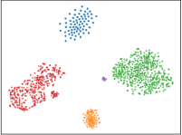
Figure 9: The t-SNE result of our model under the five-degradation setting.

Finally, we provide more qualitative results of the all-in-one setting and single-task setting for three image restoration tasks, including image deraining, dehazing, and denoising.

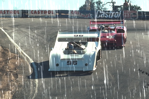
Degraded	22.95 dB	26.71 dB	30.03 dB	34.78 dB	PSNR
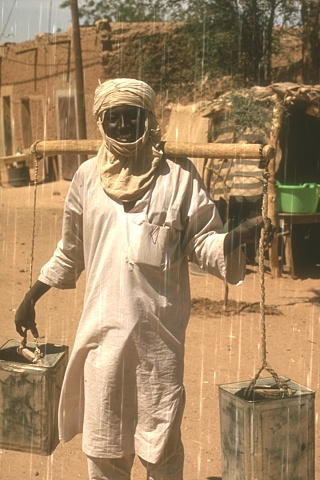
Degraded	28.61 dB	29.18 dB	31.11 dB	35.80 dB	PSNR
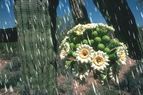
Degraded	23.08 dB	29.15 dB	32.00 dB	36.99 dB	PSNR
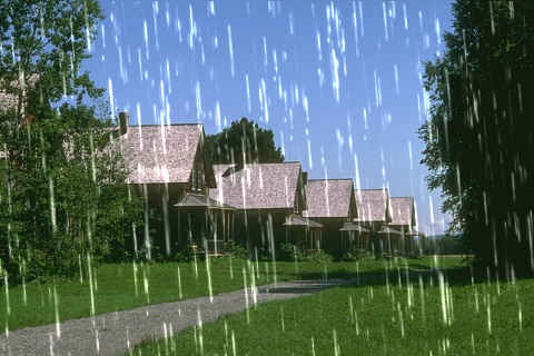
Degraded	19.97 dB	29.23 dB	29.74 dB	32.34 dB	PSNR
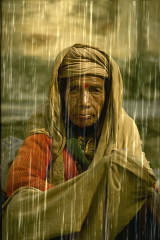
Degraded	21.09 dB	30.80 dB	34.17 dB	36.91 dB	PSNR
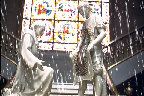
Degraded	17.49 dB	27.49 dB	28.22 dB	30.67 dB	PSNR
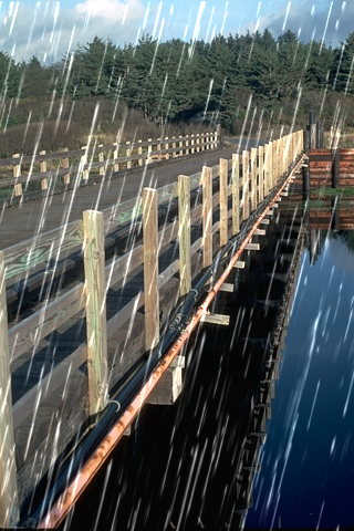
Degraded	18.00 dB	32.94 dB	33.61 dB	37.13 dB	PSNR
Degraded	25.47 dB	33.46 dB	36.80 dB	44.37 dB	PSNR
Image	Input	AirNet [33]	PromptIR [46]	Ours	Reference

Figure 10: Image deraining comparisons on Rain100L [68] under the three-degradation setting.

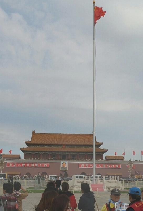
Degraded	14.65 dB	26.60 dB	27.24 dB	31.63 dB	PSNR
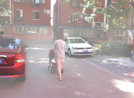
Degraded	6.58 dB	19.79 dB	24.34 dB	29.45 dB	PSNR
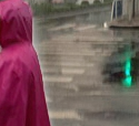
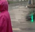
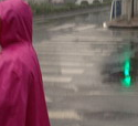
Degraded	9.61 dB	18.78 dB	25.44 dB	27.39 dB	PSNR
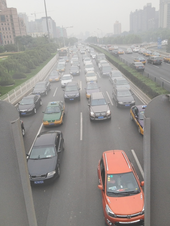
Degraded	10.49 dB	24.58 dB	24.70 dB	27.57 dB	PSNR
Image	Input	AirNet [33]	PromptIR [46]	Ours	Reference

Figure 11: Image dehazing comparisons on SOTS [32] under the three-degradation setting.

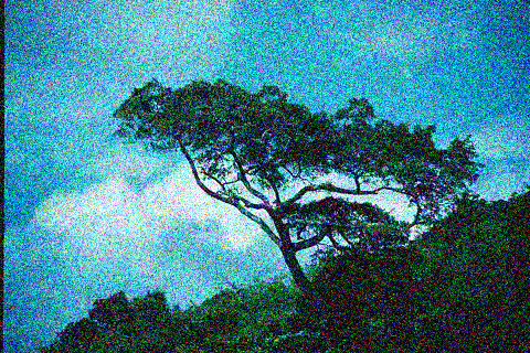
Degraded	16.49 dB	28.73 dB	28.77 dB	29.09 dB	PSNR
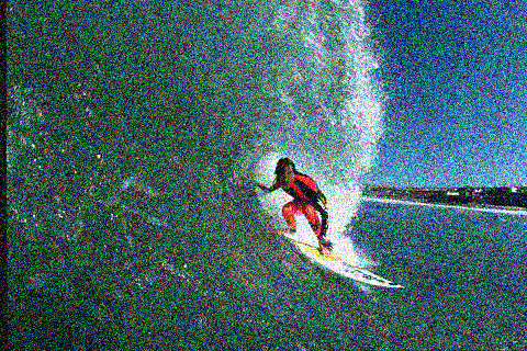
Degraded	15.13 dB	31.68 dB	31.50 dB	31.99 dB	PSNR
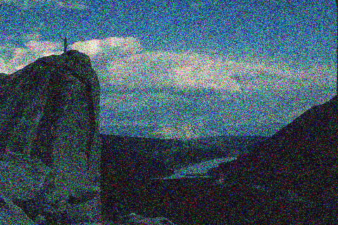
Degraded	16.90 dB	36.02 dB	34.08 dB	36.31 dB	PSNR
Image	Input	AirNet [33]	PromptIR [46]	Ours	Reference

Figure 12: Image denoising comparisons on BSD68 [41] with $\sigma=50$ under the three-degradation setting.

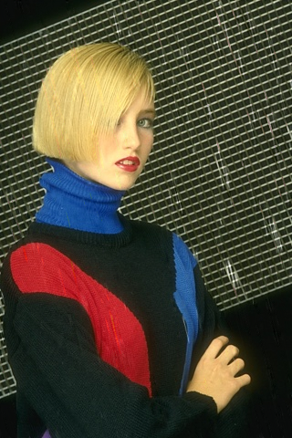
19.98 dB	18.85 dB	32.11 dB	PSNR
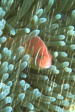
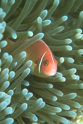
20.30 dB	35.08 dB	42.86 dB	PSNR
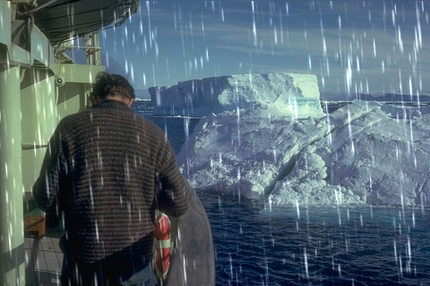
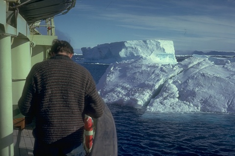
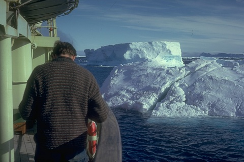
24.13 dB	33.50 dB	39.66 dB	PSNR
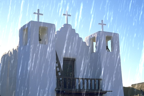
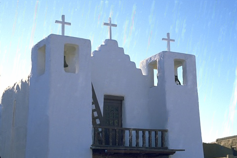
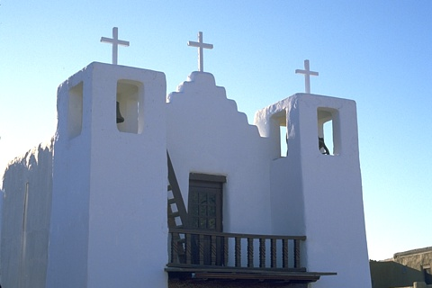
26.29 dB	35.39 dB	42.68 dB	PSNR
21.61 dB	31.30 dB	35.57 dB	PSNR
Rainy Image	AirNet [33]	Ours	Reference

Figure 13: Image draining comparisons under the single task setting on Rain100L [68].

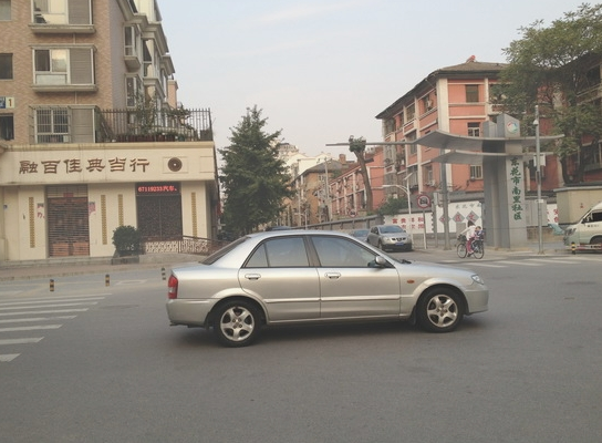
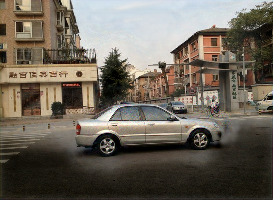
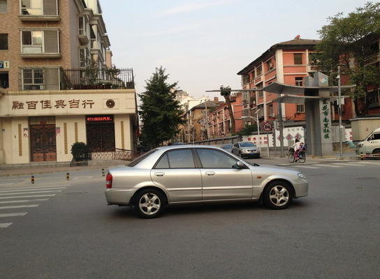
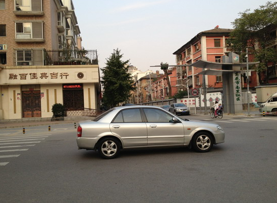
19.58 dB	17.81 dB	37.40 dB	PSNR
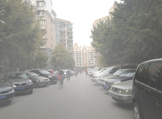
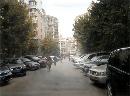
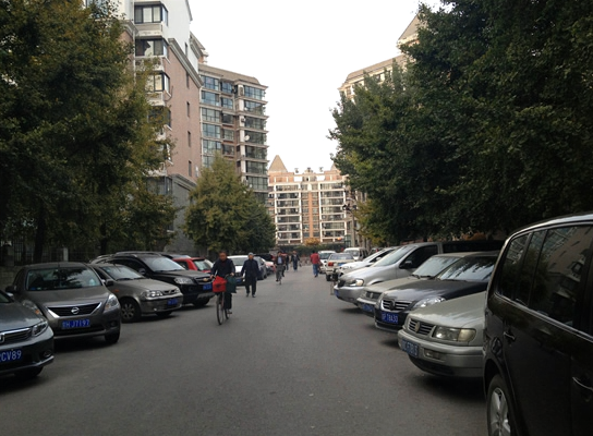
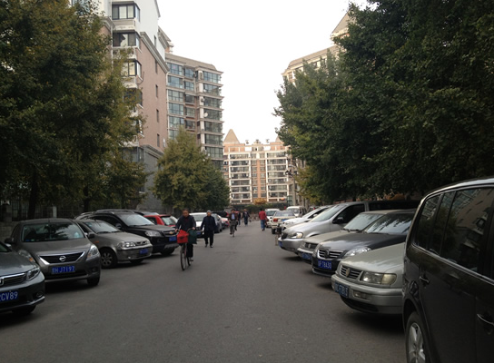
10.58 dB	20.12 dB	33.24 dB	PSNR
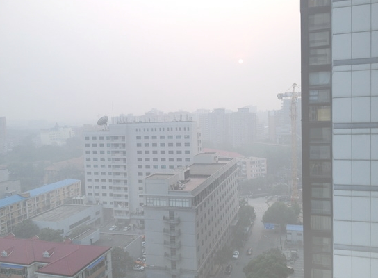
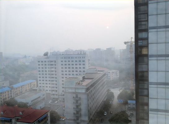
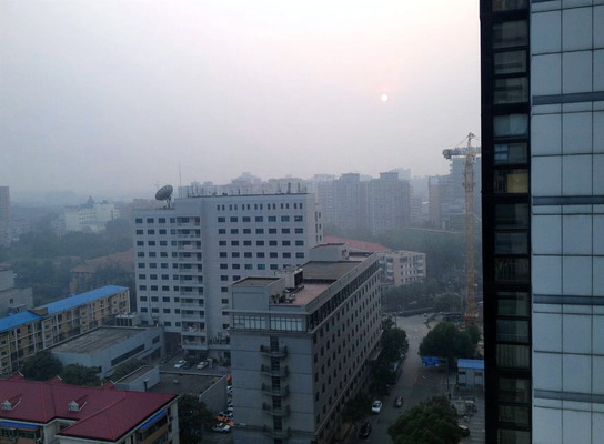
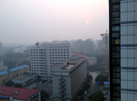
11.05 dB	15.59 dB	32.96 dB	PSNR
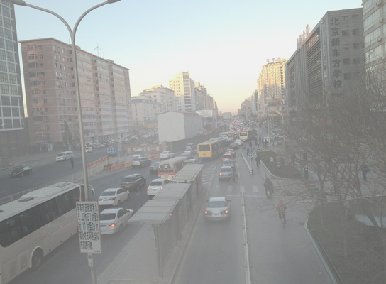
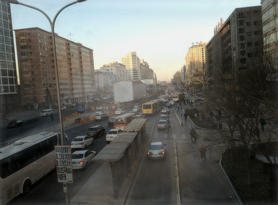
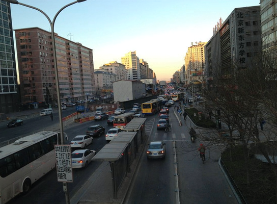
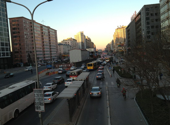
10.09 dB	21.28 dB	34.13 dB	PSNR
9.97 dB	17.61 dB	30.27 dB	PSNR
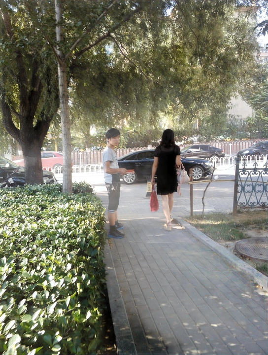
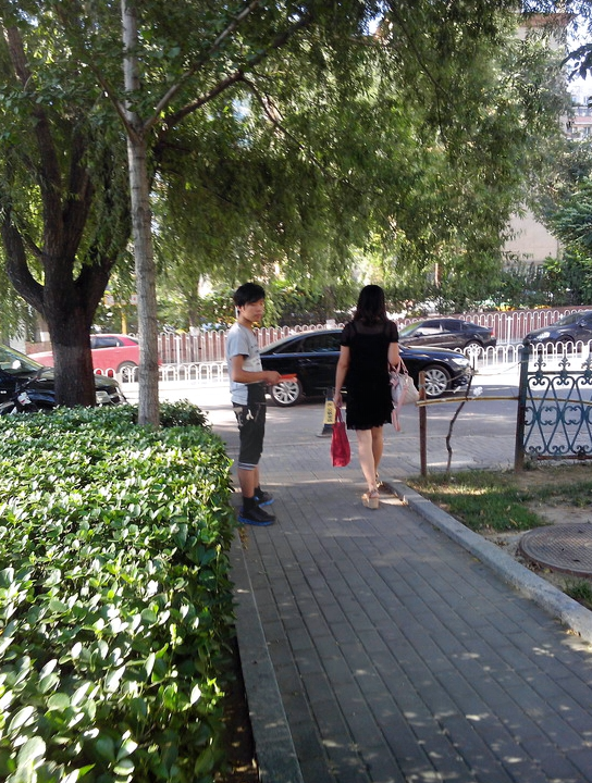
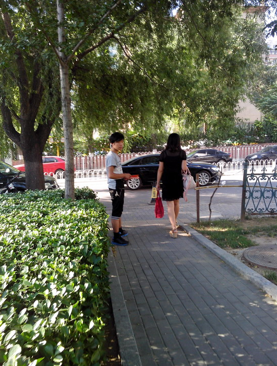
10.86 dB	16.98 dB	29.61 dB	PSNR
Hazy Image	AirNet [33]	Ours	Reference

Figure 14: Image dehazing comparisons under the single task setting on SOTS [32].

Noisy	14.49 dB	27.49 dB	28.69 dB	PSNR
Noisy	14.58 dB	31.97 dB	32.57 dB	PSNR
Noisy	14.69 dB	29.18 dB	31.17 dB	PSNR
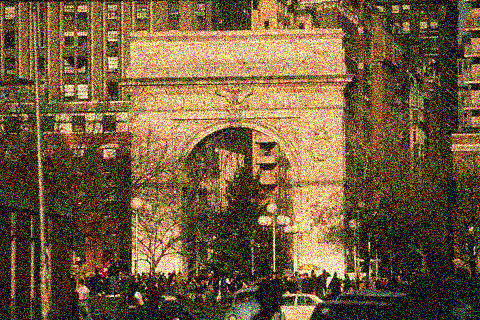
Noisy	15.08 dB	26.73 dB	27.31 dB	PSNR
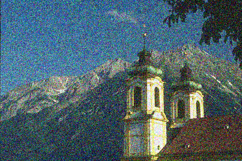
Noisy	14.87 dB	29.25 dB	29.75 dB	PSNR
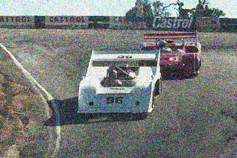
Noisy	14.62 dB	29.74 dB	30.44 dB	PSNR
Noisy	14.83 dB	29.87 dB	30.19 dB	PSNR
Image	Input	AirNet [33]	Ours	Reference

Figure 15: Image denoising results under single task setting on BSD68 [41] with $\sigma=50$.

References

- [1] Ai, Y., Huang, H., Zhou, X., Wang, J., He, R.: Multimodal prompt perceiver: Empower adaptiveness, generalizability and fidelity for all-in-one image restoration. arXiv:2312.02918 (2023)
- [2] Arbelaez, P., Maire, M., Fowlkes, C., Malik, J.: Contour detection and hierarchical image segmentation. TPAMI (2010)
- [3] Ba, J.L., Kiros, J.R., Hinton, G.E.: Layer normalization. arXiv:1607.06450 (2016)
- [4] Berman, D., Avidan, S., et al.: Non-local image dehazing. In: CVPR (2016)
- [5] Brown, T., Mann, B., Ryder, N., Subbiah, M., Kaplan, J.D., Dhariwal, P., Neelakantan, A., Shyam, P., Sastry, G., Askell, A., et al.: Language models are few-shot learners. NeurIPS (2020)
- [6] Cai, B., Xu, X., Jia, K., Qing, C., Tao, D.: Dehazenet: An end-to-end system for single image haze removal. TIP (2016)
- [7] Chen, C.F.R., Fan, Q., Panda, R.: Crossvit: Cross-attention multi-scale vision transformer for image classification. In: ICCV (2021)
- [8] Chen, H., Wang, Y., Guo, T., Xu, C., Deng, Y., Liu, Z., Ma, S., Xu, C., Xu, C., Gao, W.: Pre-trained image processing transformer. In: CVPR (2021)
- [9] Chen, L., Chu, X., Zhang, X., Sun, J.: Simple baselines for image restoration. In: ECCV (2022)
- [10] Chen, L., Lu, X., Zhang, J., Chu, X., Chen, C.: Hinet: Half instance normalization network for image restoration. In: CVPR Workshops (2021)
- [11] Chen, W.T., Fang, H.Y., Hsieh, C.L., Tsai, C.C., Chen, I., Ding, J.J., Kuo, S.Y., et al.: All snow removed: Single image desnowing algorithm using hierarchical dual-tree complex wavelet representation and contradict channel loss. In: ICCV (2021)
- [12] Chen, Y.W., Pei, S.C.: Always clear days: Degradation type and severity aware all-in-one adverse weather removal. arXiv:2310.18293 (2023)
- [13] Cho, S.J., Ji, S.W., Hong, J.P., Jung, S.W., Ko, S.J.: Rethinking coarse-to-fine approach in single image deblurring. In: ICCV (2021)
- [14] Conde, M.V., Geigle, G., Timofte, R.: High-quality image restoration following human instructions. arXiv:2401.16468 (2024)
- [15] Cui, Y., Ren, W., Cao, X., Knoll, A.: Focal network for image restoration. In: ICCV (2023)
- [16] Cui, Y., Tao, Y., Ren, W., Knoll, A.: Dual-domain attention for image deblurring. In: AAAI (2023)
- [17] Dabov, K., Foi, A., Katkovnik, V., Egiazarian, K.: Color image denoising via sparse 3d collaborative filtering with grouping constraint in luminance-chrominance space. In: ICIP (2007)
- [18] Dong, H., Pan, J., Xiang, L., Hu, Z., Zhang, X., Wang, F., Yang, M.H.: Multi-scale boosted dehazing network with dense feature fusion. In: CVPR (2020)
- [19] Dong, W., Zhang, L., Shi, G., Wu, X.: Image deblurring and super-resolution by adaptive sparse domain selection and adaptive regularization. TIP (2011)
- [20] Dong, Y., Liu, Y., Zhang, H., Chen, S., Qiao, Y.: Fd-gan: Generative adversarial networks with fusion-discriminator for single image dehazing. In: AAAI (2020)
- [21] Fan, Q., Chen, D., Yuan, L., Hua, G., Yu, N., Chen, B.: A general decoupled learning framework for parameterized image operators. TPAMI (2019)
- [22] Gao, H., Tao, X., Shen, X., Jia, J.: Dynamic scene deblurring with parameter selective sharing and nested skip connections. In: CVPR (2019)
- [23] Guo, C.L., Yan, Q., Anwar, S., Cong, R., Ren, W., Li, C.: Image dehazing transformer with transmission-aware 3d position embedding. In: CVPR (2022)
- [24] He, K., Sun, J., Tang, X.: Single image haze removal using dark channel prior. TPAMI (2010)
- [25] Huang, J.B., Singh, A., Ahuja, N.: Single image super-resolution from transformed self-exemplars. In: CVPR (2015)
- [26] Jiang, K., Wang, Z., Yi, P., Chen, C., Huang, B., Luo, Y., Ma, J., Jiang, J.: Multi-scale progressive fusion network for single image deraining. In: CVPR (2020)
- [27] Jiang, Y., Zhang, Z., Xue, T., Gu, J.: Autodir: Automatic all-in-one image restoration with latent diffusion. arXiv:2310.10123 (2023)
- [28] Kim, K.I., Kwon, Y.: Single-image super-resolution using sparse regression and natural image prior. TPAMI (2010)
- [29] Kopf, J., Neubert, B., Chen, B., Cohen, M., Cohen-Or, D., Deussen, O., Uyttendaele, M., Lischinski, D.: Deep photo: Model-based photograph enhancement and viewing. ACM TOG (2008)
- [30] Lester, B., Al-Rfou, R., Constant, N.: The power of scale for parameter-efficient prompt tuning. In: EMNLP (2021)
- [31] Li, B., Peng, X., Wang, Z., Xu, J., Feng, D.: Aod-net: All-in-one dehazing network. In: ICCV (2017)
- [32] Li, B., Ren, W., Fu, D., Tao, D., Feng, D., Zeng, W., Wang, Z.: Benchmarking single-image dehazing and beyond. TIP (2018)
- [33] Li, B., Liu, X., Hu, P., Wu, Z., Lv, J., Peng, X.: All-in-one image restoration for unknown corruption. In: CVPR (2022)
- [34] Li, R., Tan, R.T., Cheong, L.F.: All in one bad weather removal using architectural search. In: CVPR (2020)
- [35] Li, Y., Fan, Y., Xiang, X., Demandolx, D., Ranjan, R., Timofte, R., Van Gool, L.: Efficient and explicit modelling of image hierarchies for image restoration. In: CVPR (2023)
- [36] Liang, J., Cao, J., Sun, G., Zhang, K., Van Gool, L., Timofte, R.: SwinIR: Image restoration using swin transformer. In: ICCV Workshops (2021)
- [37] Liu, J., Wu, H., Xie, Y., Qu, Y., Ma, L.: Trident dehazing network. In: CVPR Workshops (2020)
- [38] Liu, L., Xie, L., Zhang, X., Yuan, S., Chen, X., Zhou, W., Li, H., Tian, Q.: Tape: Task-agnostic prior embedding for image restoration. In: ECCV (2022)
- [39] Ma, J., Cheng, T., Wang, G., Zhang, Q., Wang, X., Zhang, L.: Prores: Exploring degradation-aware visual prompt for universal image restoration. arXiv:2306.13653 (2023)
- [40] Ma, K., Duanmu, Z., Wu, Q., Wang, Z., Yong, H., Li, H., Zhang, L.: Waterloo exploration database: New challenges for image quality assessment models. TIP (2016)
- [41] Martin, D., Fowlkes, C., Tal, D., Malik, J.: A database of human segmented natural images and its application to evaluating segmentation algorithms and measuring ecological statistics. In: ICCV (2001)
- [42] Michaeli, T., Irani, M.: Nonparametric blind super-resolution. In: ICCV (2013)
- [43] Mou, C., Wang, Q., Zhang, J.: Deep generalized unfolding networks for image restoration. In: CVPR (2022)
- [44] Nah, S., Hyun Kim, T., Mu Lee, K.: Deep multi-scale convolutional neural network for dynamic scene deblurring. In: CVPR (2017)
- [45] Nah, S., Son, S., Lee, J., Lee, K.M.: Clean images are hard to reblur: Exploiting the ill-posed inverse task for dynamic scene deblurring. In: ICLR (2022)
- [46] Potlapalli, V., Zamir, S.W., Khan, S.H., Shahbaz Khan, F.: Promptir: Prompting for all-in-one image restoration. NeurIPS (2023)
- [47] Qin, X., Wang, Z., Bai, Y., Xie, X., Jia, H.: Ffa-net: Feature fusion attention network for single image dehazing. In: AAAI (2020)
- [48] Qu, Y., Chen, Y., Huang, J., Xie, Y.: Enhanced pix2pix dehazing network. In: CVPR (2019)
- [49] Ren, C., He, X., Wang, C., Zhao, Z.: Adaptive consistency prior based deep network for image denoising. In: CVPR (2021)
- [50] Ren, D., Zuo, W., Hu, Q., Zhu, P., Meng, D.: Progressive image deraining networks: A better and simpler baseline. In: CVPR (2019)
- [51] Ren, W., Liu, S., Zhang, H., Pan, J., Cao, X., Yang, M.H.: Single image dehazing via multi-scale convolutional neural networks. In: ECCV (2016)
- [52] Ren, W., Pan, J., Zhang, H., Cao, X., Yang, M.H.: Single image dehazing via multi-scale convolutional neural networks with holistic edges. IJCV (2020)
- [53] Rich, F.: Kodak lossless true color image suite. http://r0k.us/graphics/kodak (1999)
- [54] Shrivastava, D., Larochelle, H., Tarlow, D.: Repository-level prompt generation for large language models of code. In: ICML (2023)
- [55] Song, Y., He, Z., Qian, H., Du, X.: Vision transformers for single image dehazing. TIP (2023)
- [56] Tian, C., Xu, Y., Zuo, W.: Image denoising using deep cnn with batch renormalization. Neural Networks (2020)
- [57] Timofte, R., De Smet, V., Van Gool, L.: Anchored neighborhood regression for fast example-based super-resolution. In: ICCV (2013)
- [58] Tsai, F.J., Peng, Y.T., Lin, Y.Y., Tsai, C.C., Lin, C.W.: Stripformer: Strip transformer for fast image deblurring. In: ECCV (2022)
- [59] Tsai, F.J., Peng, Y.T., Tsai, C.C., Lin, Y.Y., Lin, C.W.: BANet: A blur-aware attention network for dynamic scene deblurring. TIP (2022)
- [60] Tu, Z., Talebi, H., Zhang, H., Yang, F., Milanfar, P., Bovik, A., Li, Y.: MAXIM: Multi-axis MLP for image processing. In: CVPR (2022)
- [61] Valanarasu, J.M.J., Yasarla, R., Patel, V.M.: Transweather: Transformer-based restoration of images degraded by adverse weather conditions. In: CVPR (2022)
- [62] Wang, Z., Cun, X., Bao, J., Zhou, W., Liu, J., Li, H.: Uformer: A general u-shaped transformer for image restoration. In: CVPR (2022)
- [63] Wang, Z., Bovik, A.C., Sheikh, H.R., Simoncelli, E.P.: Image quality assessment: from error visibility to structural similarity. TIP (2004)
- [64] Wei, C., Wang, W., Yang, W., Liu, J.: Deep retinex decomposition for low-light enhancement. arXiv:1808.04560 (2018)
- [65] Wei, W., Meng, D., Zhao, Q., Xu, Z., Wu, Y.: Semi-supervised transfer learning for image rain removal. In: CVPR (2019)
- [66] Woo, S., Park, J., Lee, J.Y., So Kweon, I.: Cbam: Convolutional block attention module. In: ECCV (2018)
- [67] Yang, H., Pan, L., Yang, Y., Liang, W.: Language-driven all-in-one adverse weather removal. arXiv:2312.01381 (2023)
- [68] Yang, W., Tan, R.T., Feng, J., Guo, Z., Yan, S., Liu, J.: Joint rain detection and removal from a single image with contextualized deep networks. TPAMI (2019)
- [69] Yasarla, R., Patel, V.M.: Uncertainty guided multi-scale residual learning-using a cycle spinning cnn for single image de-raining. In: CVPR (2019)
- [70] Zamir, S.W., Arora, A., Khan, S., Hayat, M., Khan, F.S., Yang, M.H.: Restormer: Efficient transformer for high-resolution image restoration. In: CVPR (2022)
- [71] Zamir, S.W., Arora, A., Khan, S., Hayat, M., Khan, F.S., Yang, M.H., Shao, L.: CycleISP: Real image restoration via improved data synthesis. In: CVPR (2020)
- [72] Zamir, S.W., Arora, A., Khan, S., Hayat, M., Khan, F.S., Yang, M.H., Shao, L.: Learning enriched features for real image restoration and enhancement. In: ECCV (2020)
- [73] Zamir, S.W., Arora, A., Khan, S., Hayat, M., Khan, F.S., Yang, M.H., Shao, L.: Multi-stage progressive image restoration. In: CVPR (2021)
- [74] Zamir, S.W., Arora, A., Khan, S., Hayat, M., Khan, F.S., Yang, M.H., Shao, L.: Learning enriched features for fast image restoration and enhancement. TPAMI (2022)
- [75] Zhang, H., Patel, V.M.: Density-aware single image de-raining using a multi-stream dense network. In: CVPR (2018)
- [76] Zhang, J., Huang, J., Yao, M., Yang, Z., Yu, H., Zhou, M., Zhao, F.: Ingredient-oriented multi-degradation learning for image restoration. In: CVPR (2023)
- [77] Zhang, K., Zuo, W., Chen, Y., Meng, D., Zhang, L.: Beyond a gaussian denoiser: Residual learning of deep cnn for image denoising. TIP (2017)
- [78] Zhang, K., Zuo, W., Gu, S., Zhang, L.: Learning deep CNN denoiser prior for image restoration. In: CVPR (2017)
- [79] Zhang, K., Zuo, W., Zhang, L.: Ffdnet: Toward a fast and flexible solution for cnn-based image denoising. TIP (2018)
- [80] Zhang, K., Luo, W., Zhong, Y., Ma, L., Stenger, B., Liu, W., Li, H.: Deblurring by realistic blurring. In: CVPR (2020)
- [81] Zhang, K., Ren, W., Luo, W., Lai, W.S., Stenger, B., Yang, M.H., Li, H.: Deep image deblurring: A survey. IJCV (2022)