Miscibility-Immiscibility transition of strongly interacting bosonic mixtures in optical lattices
Abstract
Interaction plays key role in the mixing properties of a multi-component system.The miscibility-immiscibility transition (MIT) in a weakly interacting mixture of Bose gases is predominantly determined by the strengths of the intra and inter-component two-body contact interactions. On the other hand, in the strongly interacting regime interaction induced processes become relevant. Despite previous studies on bosonic mixtures in optical lattices, the effects of the interaction induced processes on the MIT remains unexplored. In this work, we investigate the MIT in the strongly interacting phases of two-component bosonic mixture trapped in a homogeneous two-dimensional square optical lattice. Particularly we examine the transition when both the components are in superfluid (SF), one-body staggered superfluid (OSSF) or supersolid (SS) phases. Our study prevails that, similar to the contact interactions, the MIT can be influenced by competing intra and inter-component density-induced tunnelings and off-site interactions. To probe the MIT in the strongly interacting regime, we study the extended version of the Bose-Hubbard model with the density induced tunneling and nearest-neighbouring interaction terms, and focus in the regime where the hopping processes are considerably weaker than the on-site interaction. We solve this model through site-decoupling mean-field theory with Gutzwiller ansatz and characterize the miscibility through the site-wise co-existence of the two-component across the lattice. Our study contributes to the better understanding of miscibility properties of multi-component systems in the strongly interacting regime.
I Introduction
Miscibility-Immiscibility transition (MIT) is ubiquitous in nature. Depending on the interaction of microscopic constituents, like van der Waals force between the molecules, some fluids may mix with each other whether others do not. Physical properties of these multi-component fluids, such as, temperature, density, pressure, etc., and external forces are conventionally known to influence the mixing properties. Intrigued by its simplicity with vast range of interdisciplinary implications Sabbatini et al. (2011), MITs have been explored extensively in quantum fluids particularly with trapped ultracold gases of atoms in the weakly interacting regime Hall et al. (1998); Mertes et al. (2007); Papp et al. (2008); Tojo et al. (2010); McCarron et al. (2011); Wacker et al. (2015); Wang et al. (2016); Eto et al. (2016). These multi-component systems can be composed of atoms of different elements Modugno et al. (2001, 2002); Lercher et al. (2011); McCarron et al. (2011); Pasquiou et al. (2013); Wacker et al. (2015); Wang et al. (2016); Cavicchioli et al. (2022), different hyperfine states Myatt et al. (1997); Hall et al. (1998); Stamper-Kurn et al. (1998); Stenger et al. (1998); Maddaloni et al. (2000); Delannoy et al. (2001); Sadler et al. (2006); Mertes et al. (2007); Anderson et al. (2009); Tojo et al. (2010); Eto et al. (2016); Fava et al. (2018); Farolfi et al. (2020, 2021); Cominotti et al. (2022) or isotopes Papp et al. (2008); Händel et al. (2011); Sugawa et al. (2011) of same element, or even elements obeying different quantum statistics Ferrier-Barbut et al. (2014); DeSalvo et al. (2017, 2019). In a multitude of previous studies, effects of system characteristics, e.g., confining potentials Gautam and Angom (2010, 2011), number-imbalance Pattinson et al. (2013); Lee et al. (2016); Wen et al. (2020), temperature Nho and Landau (2007); Roy et al. (2014); Roy and Angom (2015); Lee et al. (2016); Suthar and Angom (2017); Ota et al. (2019); Roy et al. (2021); Spada et al. (2023), impurity and topological defects Bandyopadhyay et al. (2017); Kuopanportti et al. (2019) on the MITs of superfluids, also referred to as phase-separation Ao and Chui (1998); Timmermans (1998); Pu and Bigelow (1998), have been explored. In such weakly interacting systems, the MITs are mainly determined by the competition between the short-ranged interactions of the components Ho and Shenoy (1996); Ao and Chui (1998); Pu and Bigelow (1998); Pethick and Smith (2002).
By restricting the atoms to interact in the wells of deep optical lattices, the effective strength of the interaction can be made significantly strong admitting novel quantum phase transitions Morsch and Oberthaler (2006); Bloch et al. (2008); Lewenstein et al. (2012); Gross and Bloch (2017). In this regime, interaction induced processes are known to influence the physical characteristics of the system, and in some cases can stabilize new quantum phases resulting significant modifications to the phase diagrams Mazzarella et al. (2006); Dutta et al. (2015). Here, we explore the role of different interactions on the MITs of bosonic multi-component systems in the strongly interacting regime.
For past two decades, the trapped ultracold atoms have been in the forefront of quantum simulation and exploration of synthetic quantum matters Lewenstein et al. (2012); Bloch et al. (2012); Gross and Bloch (2017). Excellent experimental control, e.g., near perfect state initialization Yang et al. (2020a, b); Ebadi et al. (2021) to the readout at the level of individual atoms Bakr et al. (2009); Kuhr (2016), has made these systems popular platforms to probe plethora of models ranging from condensed-matter physics Jaksch and Zoller (2005); Lewenstein et al. (2007); Zhang et al. (2018); Hofstetter and Qin (2018); Tarruell and Sanchez-Palencia (2018), high-energy physics Wiese (2013); Aidelsburger et al. (2022); Zohar et al. (2015); Halimeh et al. (2023), quantum information Monroe (2002); Jaksch (2004); García-Ripoll et al. (2005), nuclear physics Gezerlis and Carlson (2008); Strinati et al. (2018), cosmology Hung et al. (2013); Schmiedmayer and Berges (2013); Chatrchyan et al. (2021) to quantum gravity Wei and Sedrakyan (2021); Uhrich et al. (2023). Under the assumption of lowest-band approximation, the minimal model which can capture the physics of an optical lattice with ultracold bosonic atoms is the bosonic version of the Hubbard model, a.k.a. the Bose-Hubbard model (BHM) Hubbard (1963); Fisher et al. (1989); Jaksch et al. (1998), where the tunneling between the nearest-neighbour wells and only the onsite interaction is considered Fisher et al. (1989); Jaksch et al. (1998). This model has been tremendously successful in describing the Superfluid (SF) to Mott-insulator (MI) transition Greiner et al. (2002); Bakr et al. (2010). However, the model demands an extension through the inclusion of other processes, such as offsite interactions, density-induced and pair tunneling, etc. Mazzarella et al. (2006), when the interaction between the atoms is stronger yielding multi-band processes and long-range interactions relevant Sowiński et al. (2012); Lühmann et al. (2012); Jürgensen et al. (2012); Maik et al. (2013); Jürgensen et al. (2014, 2015); Lühmann (2016); Dutta et al. (2015). Such extended versions of the BHM are known to exhibit other phases, for example, density-wave (DW) Mazzarella et al. (2006), supersolid (SS) Sengupta et al. (2005); Scarola and Das Sarma (2005); Ng and Chen (2008); Iskin (2011); Suthar et al. (2020a), staggered superfluids and supersolids Johnstone et al. (2019); Suthar et al. (2020b); Suthar and Ng (2022), etc., in the regime where the onsite interaction is either comparable or sufficiently larger than the tunneling process. Additionally, these processes also known to influence the existing characteristics of the BHM, like the SF-MI transition Jürgensen et al. (2012); Baier et al. (2016).
In general, the long-range interactions and density induced tunneling (DIT) processes have implications in fast-information scrambling and quantum-many body chaos Chowdhury et al. (2022); Bandyopadhyay et al. (2023), spin glasses and quantum annealing algorithms Panchenko (2015); Lechner et al. (2015) to the understanding properties of superconductors and magnetic materials Pu et al. (2001); de Paz et al. (2013). While modeling the optical lattice systems, the non-local interactions and DIT are often restricted to the nearest-neighbouring (NN) sites to incorporate the leading order effects. Although these processes may become relevant for strong enough onsite interaction, they become particularly important for atoms or molecules with large dipole moment Góral et al. (2002); Danshita and Sá de Melo (2009); Capogrosso-Sansone et al. (2010); Sowiński et al. (2012); Maik et al. (2013); Baier et al. (2016); Bandyopadhyay et al. (2019). Motivated by the intriguing aspects of these processes and experimental progresses on optical lattice systems with bososnic dipolar atoms Baier et al. (2016) and molecules Reichsöllner et al. (2017), here we explore the effects of nearest-neighbour interaction and DIT on the MITs of two-component bosonic mixtures in the optical lattices. In particular, we investigate the MIT in the different SF and SS phases in the strongly interacting regime, and reveal the role of the DIT and NN-interaction on the immiscibility criterion.
The key result of this manuscript is summarized in the Fig. 2 (see Sec.III), which we subsequently extend to large range of parameter domains. The readers familiar with the two-component version of extended BHM and single-site mean-field techniques to solve the model, may like to skip the Secs. II. For better readability, we organize the manuscript as follows: In Sec. II, we first discuss the model Hamiltonian for ultracold two-component mixtures of bosonic particles in the presence of different interaction induced processes. Then, we elaborate on the mean-field framework (Sec. II.1) and numerical methodology (Sec. II.2), which we employ to solve the model. Afterwards, we discuss several order parameters used to characterize of different phases exhibited by the model (Sec. II.3). In Sec. III we discuss the MIT of SF, OSSF and SS phases with respect to the DIT processes and NN interactions. We extend our results by examining the influence of these processes on the immiscibility condition in Sec. IV. In this section, we additionally present the phase diagrams of the model with DIT processes (Sec. IV.1) and both DIT processes and NN interactions (Sec. IV.3). Finally, we summarize our key findings and highlight experimental feasibility of our observations in Sec. V.
II Model
To study the MIT, we consider a system comprising two-component mixture of bosonic particles trapped in the potential of a two-dimensional (2D) optical lattice comprising sites. Under the second quantization framework, the grand canonical Hamiltonian of such a system is given by
| (1) |
where
| (2) | |||||
In Eqs. (1) and (2), the first term, , corresponds to the standard two-component BHM Hamiltonian, where , stands as the component index, and , denote the lattice site indices of a square lattice with the notation representing NN sites. The local creation, annihilation and number operators of the th site are denoted by , and , respectively. corresponds to the strength of the hopping process of particles within NN sites, is the strength of the onsite repulsive contact interaction of individual component, and is the inter-component onsite interaction strength. We consider all these strengths positive, uniform and isotropic, and probe the regime when is sufficiently smaller than . The chemical potential enforces the particle number conservation in the grand-canonical ensemble, and determine the fillings of individual component in the lattice system. In the present work, we fix . Therefore, we consider the two-component BHM with symmetric hopping, on-site interactions and chemical potentials.
In the strongly interacting regime, , the single component BHM exhibits a quantum phase transition between the MI and SF phases stemming from the competition of the hopping and onsite interaction processes. The system exhibits insulating MI phases of different fillings determined by in the strongly interacting limit, . While in the weakly interacting regime it is in the SF phase. The two-component version of the BHM has also been studied in earlier works, and known to host additional paired and anti paired phases Kuklov and Svistunov (2003); Kuklov et al. (2004). In the strongly interacting regime, the phase diagram can have parameter domains of nontrivial MI lobes with half-integer total filling alongside the SF and usual two-component MI lobes of integer total filling Isacsson et al. (2005); Bai et al. (2020). Additionally, in this regime the two-component BHM for different fillings can be mapped to a plethora of spin Hamiltonians Altman et al. (2003); Kuklov and Svistunov (2003), and thus the two-component mixtures of ultracold atoms in the optical lattices have potential applications as quantum simulator of various spin models Morera et al. (2019).
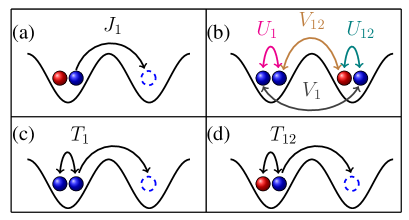
The second term in Eqs. (1) and (2), , is the Hamiltonian part representing DIT processes of the two-components Jürgensen et al. (2012); Lühmann et al. (2012); Sowiński et al. (2012); Maik et al. (2013). Here, and correspond to the intra and inter-component DIT strengths, respectively. For large onsite interaction, the DIT can stem from interaction induced band mixing Dutta et al. (2011); Lühmann et al. (2012); Maik et al. (2013), and the process can be sufficiently strong for other interactions, such as, dipole-dipole interaction Sowiński et al. (2012). The inclusion of DIT term in the BHM modifies the phase diagram significantly in the strongly interacting regime and for large . The effect of the latter is intuitively expected as the hopping process is enhanced with increasing filling resulting destruction of certain insulating phases in favor of superfluidity. Additionally, the system is known to exhibit a superfluid phase with uniform density but sign staggering in the phase of the SF order parameter, which is referred to as one body staggered superfluid (OSSF) phase Johnstone et al. (2019). This staggered phase is a mean-field incarnation of the novel twisted SF phase having time-reversal symmetry broken complex SF order parameter, and this phase is known to be better stabilized in the multi-component system of bosons Soltan-Panahi et al. (2012).
The third term in Eqs. (1) and (2), , stands for the density-density interaction between the particles in the NN sites. For a system of strong enough contact interaction this process can be relevant, but it is weaker in strength than the DIT process Mazzarella et al. (2006). On the other hand, this interaction can be strong for atoms or molecules with large dipole moments. Then, the particles in different sites can interact through long-range dipole-dipole interaction of which the range can be limited to the NN sites to capture the effects of the strongest off-site interaction Baier et al. (2016); Bandyopadhyay et al. (2019, 2022). Such a model with NN density-density interaction is traditionally been termed as extended BHM (eBHM) Kühner et al. (2000); Sengupta et al. (2005); Scarola and Das Sarma (2005); Mazzarella et al. (2006); Ng and Chen (2008); Iskin (2011); Suthar et al. (2020a), and it is experimentally studied with magnetic Er atoms in a 3D cubic and multi-layers of 2D optical lattice in the context of MI-SF transition Baier et al. (2016). In the equations, and are the strengths of intra and inter-component NN interactions, and potential realization of the two-component version of the eBHM can be made with the mixture of dipolar atoms or molecules Trautmann et al. (2018). In the presence of NN interaction, the eBHM can withstand quantum phases with broken lattice transnational symmetry, such as, DW and SS. With the inclusion of the DIT process, the eBHM can furthermore stabilize one body staggered supersolid (OSSS) phase, which has the density modulation alongside the sign staggering in the phase of the SF order parameter. Note that the Hamiltonian in Eqs. (1) and (2), has symmetry due to the conservation of total particle number of each component. Additionally, for symmetric choice of intra-component parameters, the Hamiltonian has additional exchange symmetry. The mean-field framework, which we employ to solve the model, explicitly breaks the symmetry, and thereby introduce the SF order parameters into the Hamiltonian depicting the number fluctuations.
In Fig. 1, we schematically illustrate the different processes described by the model Hamiltonian in Eqs. (1) and (2). The Hamiltonian can additionally be extended via incorporating pair hopping processes yielding novel phases of particle pairs, e.g., pair superfluids and supersolids. But, such processes are weaker than the DIT processes for systems with short-ranged interacting particles Mazzarella et al. (2006); Johnstone et al. (2019). Even for the systems comprising dipolar particles the pair hopping process is weaker than the DIT and NN interactions Sowiński et al. (2012). Therefore, in this work we restrict the extension of the BHM considering the latter two processes.
II.1 Solving the model: Mean field theory
In our study, we employ single-site mean-field theory to obtain the ground states of the Hamiltonian in Eqs. (1) and (2) Rokhsar and Kotliar (1991); Sheshadri et al. (1993); Anufriiev and Zaleski (2016); Bai et al. (2018); Bandyopadhyay et al. (2019); Bai et al. (2020). The aim of this framework is to cast the system Hamiltonian as a sum of the local Hamiltonians of individual site. For this, the non-local terms in Eq. (2) are decoupled through the introduction of the mean-fields of different operators. In order to do so, the annihilation, creation and number operators of each site are decomposed into corresponding mean-fields and fluctuation operators, That is, , where and are the mean-field and fluctuation operator of a representative single-site operator . Then, to the leading order of the fluctuations, different terms of Eq. (2) can be written as
where the mean-field is the SF order parameter, is the local density, , , and are the order-parameters for density-dependent transport properties Johnstone et al. (2019). Now, the mean-field version of the Hamiltonian can be written as a sum of local Hamiltonians of the sites
| (3) |
For brevity, we have detailed the local mean-field Hamiltonian of a site in the Appendix (A).
The single-site Hamiltonian matrix can be constructed with respect to the local Fock basis , where is the occupation number of the -th component, and then the matrix can be diagonalized to obtain the ground state of the single-site Hamiltonian. From this, the ground state of the mean-field Hamiltonian in Eq. (3) can be constructed by employing the Gutzwiller ansatz, where the ground state of the system is expressed as the tensor product of ground states of all the local Hamiltonians, i.e.,
| (4) |
Here, is the ground state of the mean-field Hamiltonian of the -th site. For bosonic particles, the site occupancy is unrestricted, but, in practice one can restrict the occupation number . The cutoff should be chosen sufficiently large than the average density , which is in turn determined by the chemical potential . The single-site Hamiltonian matrix then becomes square matrix of dimension . The coefficients, , satisfy the normalization condition = 1.
The local SF order parameter and density of the first component can be calculated from the Gutzwiller ground state as
| (5) |
These quantities can be calculated for the second component in the similar manner. The order parameters related to the density induced transport can be calculated as
| (6) | |||||
and similarly and can be evaluated.
We note a few characteristics of these order parameters, which we utilize to explain some of our results. The Hamiltonian in Eqs. (1) and (2) is time reversal invariant. Due to the presence of only real parameters, the Hamiltonian matrix is real-symmetric, yielding real eigenstates. The corresponding single-site Hamiltonian is real-symmetric as well. This implies in Eq. (4). Then, quantities in Eqs. (5)-(6) are real. Additionally, invoking the single-site mean-field decomposition, the order parameters for density induced transport can be written as
| (7) |
Even though this decomposition is formally correct, its evaluation with respect to the state in Eq. (4) is subtle. In our analysis, being onsite term, we do not perform this decomposition and account it exactly. However, Eq. (7) demonstrates that to the leading order of the fluctuations, the expectation value of these order parameters . Now, due to , . Similarly, . We also consistently observe this characteristic in our numerical analysis.
II.2 Numerical methodology
In our numerical analysis, we obtain the ground state of the mean-field Hamiltonian self-consistently. For this purpose, we perform an iterative process where we construct the single site mean-field Hamiltonian matrix with respect to the local Fock basis, and then diagonalize it to obtain the ground state of a site. In particular, we start with an initial guess values for the mean-field quantities in the Hamiltonian given in Eqs. (3) and (10). After diagonalizing the matrix we update the mean-field quantities, of the site by new values computed using updated ground state as per Eqs. (5)-(6). Next, we perform the similar procedure for the next site, where the updated mean-fields of the previous site have been used for computation. This procedure is carried out for all the sites in the system, which constitutes a sweep. In order to obtain a self-consistent solution the above sweep is carried out until an expected convergence with respect to the values of the mean-fields is obtained. It is to be noted that our implementation is site-dependent and does not reduce to an effective single-site theory. This allow us to simulate quantum phases having spatial inhomogeneity. We consider lattice, where ranges from to , and the local occupation state of each component is restricted to . Thus, the single-site matrix dimension in our simulation is . The above cut-off is justified as we we restrict parameter regime throughout. The convergence criteria imposed to our simulation is , where subscript denotes the -th sweep. We employ periodic boundary conditions in both directions of the homogeneous 2D lattice to account the thermodynamic characteristics of the obtained quantum phases.
| Quantum phase | |||||
|---|---|---|---|---|---|
| Mott insulator (MI) | Integer | ||||
| Superfluid (SF) | Real | ||||
| Density Wave (DW) | Integer | ||||
| Super Solid (SS) | Real | ||||
| One Body Staggered Superfluid (OSSF) | Real | ||||
| One Body Staggered Super Solid (OSSS) | Real |
II.3 Characterization of quantum phases
The Hamiltonian in Eqs.(1) and (2) is expected to withstand quantum phases with both uniform and lattice transnational symmetry broken order parameters. So, we identify different quantum phases based on the combinations of values of different mean-fields and periodicity therein, which stand as order parameters in some cases under the present framework. Particularly we consider the SF order parameter, average density and the order parameter associated with the density inducted transport. Since we are working with two-component system, we compute the total SF order parameter and total density of every sites in the lattice to identify the known MI and SF phases of two-component BHM Anufriiev and Zaleski (2016); Bai et al. (2020). In the MI phases of different fillings, the SF order parameter is zero, and the system has commensurate integer density on every lattice site. Whereas, for the SF phase is non zero quantity and .
In the presence of DIT term, the BHM can withstand the OSSF phase, which can be characterized through sign staggering in the phase of SF order parameter of adjacent lattice sites, yielding a checkerboard order in the phase of for a isotropic 2D square optical lattice. To be explicit in denoting the periodicity in the phase of the SF order parameter, we adapt bipartite lattice description of checkerboard ordering: spatially periodic modulation can be considered as if the system has two sub-lattices, A and B, which are interlaced with one-site periodicity along both directions. In other words, all the NN sites of any lattice site in sub-lattice A belong to to sub-lattice B, and vice versa. Then, we can express the spatial distribution of in a compact notation as , where and are the values of the SF order parameter in A and B sub-lattices, respectively. Since, spatial profile of has checkerboard sign staggering but uniform distribution in the OSSF phase, we can express . Additionally, is real and uniform, like in the SF phase.
With the inclusion of NN density-density interaction term, the model can stabilize DW and SS phases for significant interaction strength. The DW phase, similar to the MI phase, is an insulating phase manifested by zero . However, this phase has checkerboard density distribution unlike the uniform MI phase. The SS phase, on the other hand, has the checkerboard profile in spatial distributions of both density and SF order parameters. Following the bipartite lattice notation, we can express the checkerboard pattern in the density distribution of these phases as . Furthermore, the model in the presence of both DIT and NN interaction terms can exhibit the OSSS phase, which has the checkerboard sign staggering in the phase of along with the checkerboard distribution of and . The order parameter qualitatively has similar trend as that of in all the mentioned phases, and hence, can be denoted as in the phases with spatial checkerboard distribution.
In this work, we obtain the quantum phases in a two component bosonic mixture with symmetric parameters. That is, the strengths of the hoppings, DIT processes, onsite and NN interactions, and chemical potentials of the components are equal, as mentioned earlier. Due to this, the components have identical distribution of the quantities in the miscible phase. In contrast, in the immiscible phase the components do not co-exist on same site, but they retain the spatial distribution in the separated regions of the system. To summarize, we list the characteristics of different quantum phases in the table 1. We explore the MIT in the strongly interacting regime, particularly in the SF, OSSF, SS and OSSS phases of both components. To quantify the co-existence of the components across the lattice system, we compute the miscibility parameter defined as
| (8) |
Therefore, in the immiscible phase is zero, whereas, any finite value of corresponds to partial miscibility of the components. In the regime when the components are completely miscible with density homogeneous distributions, . It is to be noted that changes from a finite value to zero continuously as the system parameters are changed to explore the MIT. At the verge of this transition, under the considered mean-field framework, we notice replenishment of one of the component at the expense of complete depopulation of the other component. This immediately yields marking the MIT. In the numerical analysis, this artifact occurs when the initial guess values of the mean-fields are chosen to be homogeneous for both components. But, with spatially asymmetric initial distributions of the mean-fields, both the components remain, and they occupy spatially separated regions in the immiscible phase. Whereas, identical distributions (homogeneous or checkerboard) of the components are retrieved in the miscible phase. Such depopulation of a component has also been observed in the context of MI-SF transition under mean-field framework Isacsson et al. (2005).
III MIT transition in the strongly interacting regime
MIT has been investigated quite extensively in the multi-component bosonic mixtures confined in continuum potentials. For such systems, the criterion of MIT is predominantly determined by the competition of the intra and inter-component contact interactions Ho and Shenoy (1996); Ao and Chui (1998); Pu and Bigelow (1998); Pethick and Smith (2002). This is further explored in shallow optical lattice systems, where both the components are in the weakly interacting SF phase. Like in the continuum systems, criterion for immiscibility is given by
| (9) |
On the other hand, in the strongly interacting regime, rich phase space structure arises for the two-component BHM Isacsson et al. (2005); Anufriiev and Zaleski (2016); Bai et al. (2018). Stemming from the competition of the hopping and contact interactions, both the components can simultaneously be in SF, MI or MI+SF phases. The latter denotes the case where one of the components is in MI phase, whereas the other component is in SF phase. Additionally, the model can withstand counter-flow SF phase and Néel ordered anti-ferromagnetic states for . However, these states are indistinguishable from the MI phase as far as , and individual SF order parameters , are concerned Altman et al. (2003); Kuklov et al. (2004); Ş G Söyler et al. (2009).
For the MIT, an analogous condition as in the Eq. (9) can be obtained, when both the components are in the MI phase Chen and Wu (2003). In earlier works considering 1D optical lattice system with sufficiently number imbalanced mixtures and strong , metastable non-overlapping emulsion states, exhibiting glassy characteristics have been investigated Roscilde and Cirac (2007); Buonsante et al. (2008). Also, immiscibility on length scales with increasing inter-component repulsion has been reported in Ref Alon et al. (2006). In the 1D BHM, MIT has been explored when both components are simultaneously MI or SF, and immiscibility condition is obtained in terms of , and Mishra et al. (2007); Zhan and McCulloch (2014); Zhan et al. (2014). Furthermore, at half-fillings of the 2D two-component BHM with symmetric hopping and interaction strengths, immiscible SF and MI phases have been found when the inter-component interaction becomes larger than the repulsive intra-component interaction Lingua et al. (2015). For unequal strengths of hopping processes, such a transition is noticed between the anti-ferromagnetic Néel state and immsicible SF phase Shrestha (2010). It is to be noted that in all these studies, the MIT is explored as a consequence of the interplay of on-site interactions, and generically a condition as in Eq. (9) has been considered as the criterion of immiscibility. But, effects of interaction induced processes, predominantly DIT and NN interaction, become relevant in the strongly interacting regime, as mentioned earlier. These are not only known to stabilize new phases and significantly modify the phase diagram, but also expected to influence usual phase transitions of the BHM. We, therefore, explore the effects of these processes on the MIT of several phases.
In an earlier work Bai et al. (2020), motivated by the experimental realization of the quantum degenerate mixture of dipolar bosonic atoms Trautmann et al. (2018), we have explored the quantum phases of two-component BHM in the presence of NN interactions. Particularly, we investigated the phases in miscible and immsicible regimes, by considering the and , respectively, and we noticed the side-by-side density distributions of different immiscible quantum phases. In this work, we numerically investigate the MIT of the strongly interacting OSSF, SF, SS and OSSS phases in the presence of interaction induced process. In particular, we explore the competing roles of the DIT processes and NN interactions in inducing the MIT of these phases.
In Fig. 2, we delineate the results on MIT by changing the strengths of intra and inter-component DIT processes and NN interactions. To steer the MIT and examine the effects of these processes, we consider . This not only allows us to scale the total Hamiltonian by , but also corresponds to the condition of immiscibility with respect to the onsite contact interaction processes. The strongly interacting regime is when the strengths of the other processes are . In this regime, we carefully choose the other parameters such that the two-component SF, OSSF and SS phases are obtained. For this, it is essential to have knowledge on the phase diagrams of the two-component BHM with the DIT processes and NN interactions. For brevity, such phase diagrams are presented in Figs. 3, 4 and 5, and explained in detail in Sec. IV. The considered values of the parameters are provided in the caption of Fig. 2.
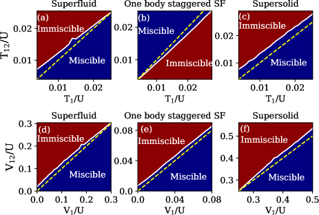
III.1 MIT with respect to DIT processes
To begin with, we consider the two-component BHM along with the DIT processes, and take . Then, for considerable strengths of DIT processes, the model can withstand the two-component OSSF phase, in addition to the two-component MI and SF phases. In Fig. 2 (a), we depict the MIT when both the components are in the SF phase. We notice that the components remain miscible as long as the inter-component DIT is weaker than the intra-component DIT processes . On the other hand, the components become immiscible for . For the convenience to read this off, we mark the by a dashed yellow line in the Fig. 2. Note that, here the condition for immiscibility is similar to Eq. (9). The Hamiltonian in Eqs. (1) and (2) has symmetry for both the components, which yields the energy functional in the even powers of the SF order parameters under the usual Landau framework Bandyopadhyay et al. (2019). In the homogeneous lattice system, the SF phase has uniform density and SF order parameter distributions. Therefore, energy contribution of the DIT processes to the energy functional is positive when the strengths are considered to be positive. This can also be understood from Eq. (A) by noting that the order parameters of the two sub-lattices are same in the uniform SF phase. In addition, the density induced transport order parameters have same sign to that of the SF order parameters, as mentioned in Sec. II.1. This yields positive mean-field energy contribution due to the DIT processes. So, the contribution from the inter-component DIT process becomes energetically costly for the miscible configuration with . As a consequence, the components become immiscible, thereby, making the contribution from the inter-component DIT process to diminish. We extend the analysis for the negative values of the DIT strengths, that is, , and observe that the system remain immiscible as long as . This is in accordance with the energy cost argument mentioned before.
On the other hand, we observe the components are immiscible when in the OSSF phase of the components [see Fig. 2 (b)]. This is in striking contrast to the trend observed in the SF phase and also to Eq. (9). The apparent opposite trend of the immiscibility condition for the positive strengths of DIT processes can be understood from the energy minimization argument. Note that the components have checkerboard sign staggering in the SF and density induced transport order parameters in the OSSF phase (see Table 1 and Sec. II.3). Therefore, the mean-field energy due to the DIT processes acquire a negative sign [see Eq. (A)]. Then, the condition for the immiscibility becomes similar to the case when the strengths are negative and the components are in the SF phase, as explained in the previous paragraph. It is known that positive DIT strength is essential to withstand the OSSF phase Johnstone et al. (2019). So, we can not explore negative DIT strengths regime for the MIT in this phase.
Next, we examine the immiscibility condition of the components when they are in the SS phase. To obtain the SS phase, we require the NN interaction term in the Hamiltonian as explained in Sec. II. We fix the NN interaction strengths and obtain the MIT condition with respect to DIT processes in the SS phases of the components, which is shown in Fig 2 (c). Here, similar to the case with SF phase, we recover the MIT condition. That is, the components become immiscible when and they are miscible when . In the SS phase, the components have checkerboard ordering in the density, SF and density induced transport order parameters. However, unlike the OSSF phase, there is no sign staggering in the order parameters (see Table 1). Therefore, the energy contribution from the intra and inter-component DIT processes is positive. Consequently, the components become immiscible when the inter-component DIT strength is larger than the intra-component strengths. The MIT condition remains similar to the SF phase when the DIT strengths are considered negative.
III.2 MIT with respect to NN interactions
Here, we examine the MIT by varying the NN interaction strengths. To explore this in the SF and SS phases of the model, the DIT processes can be set to zero, but for the OSSF phase DIT is essential. In Fig 2 (d)-(f), we depict the MIT when both components are in SF, OSSF, and SS phases, respectively. The DIT strengths are set to zero for Fig. 2 (d) and (f), but fixed to for 2 (e). In all these phases, similar to the condition in Eq. (9), the components are immiscible when and miscible for for positive strengths of the NN interactions. The energy contribution of the NN interactions is positive for the positive strengths [see Eq. (16)]. So, the components become immiscible for , to reduce the energy contribution from the inter-component NN interaction. On the other hand, for negative NN interaction strengths, that is, , the energy contribution is negative. Consequently, the components remain immiscible .
In Fig 2 we present the numerical results obtained for a lattice system of size . Increasing the lattice size further does not qualitatively change our results. We illustrate the distributions of density, SF and density induced order parameters of immsicible OSSF, SF, SS phases in the Fig. 8, Fig. 9, and Fig. 10, respectively.
IV Broadening the parameter regime
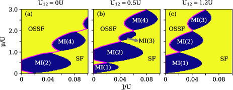
In this section, we extend our analysis on the MIT transition of the two-component system with DIT processes and NN interactions. We aim to probe the effects of these processes on the immiscibility condition in terms of the on-site interaction strengths [see Eq. (9)]. To explore this in the strongly interacting phases of the model, the knowledge of the phase diagram is essential. For single component bosons in 1D and 2D optical lattices with DIT process, the mean-field phase diagrams have been reported Johnstone et al. (2019); Suthar et al. (2020b); Suthar and Ng (2022). But, the phase diagram for the two component BHM with DIT processes has not been reported yet. Therefore, we obtain the mean-field phase diagram of a two-component BHM with DIT processes. We first present the phase diagrams in Figs. 3 (a) - (c) for different values of inter-component interaction strengths for the case when the NN interactions are absent. Later, similar phase diagrams are presented for finite NN interaction strengths in Figs. 4 (a) - (c).
IV.1 Phase diagram of two component BHM with DIT
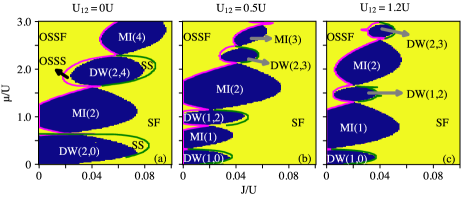
We consider a 2D square lattice of size with periodic boundary conditions to numerically obtain the phase diagrams. For this, we employ the framework explained in Secs. II.1 and II.2, and evaluate the order-parameters to characterize the various quantum phases (see Sec. II.3 and Table 1) of the model. The scale is fixed as . Then, the phase diagrams are obtained for three different values of the inter-component interaction strengths, , which are presented in Fig. 3 (a) - (c). In the absence of DIT processes, the mean-field phase diagrams of a two-component BHM have the parameter domains for two-component SF and MI phases Anufriiev and Zaleski (2016); Bai et al. (2020). The parameter domains of the MI phase of different fillings form usual Mott lobes which are marked as MI(), where . On the other hand, finite DIT processes destabilize the insulating MI phase towards OSSF phase in the strongly interacting regime. For the phase diagram simulations, we consider . In the absence of inter-component interaction, , we obtain Mott-lobes of only even integer [see Fig. 3 (a)], which we refer to as even MI lobes. These also correspond to MI lobes of integer filling. In these two-component MI phases, both the components have uniform commensurate integer occupancy and zero SF order parameter. With increasing density the hopping of the particles in the system is enhanced due to the DIT processes. Thereby, the parameter domain of the two-component OSSF phase gets larger, a characteristic also present in the single-component case Johnstone et al. (2019). The phase boundary of the OSSF phase is represented by magenta line in Fig. 3 (a) - (c).
Finite inter-component onsite interaction introduces the parameter domains for MI phases of odd integer , which form the odd MI lobes [see Fig. 3 (b) and (c)]. In these MI phases, total density distribution is uniform and integer, but the density distribution of individual component is random. The SF order parameters are zero and occupancy of each component at any site is integer. Consequently, these are incompressible phases with half-integer filling, for example, the MI(1) and MI(3) correspond to two-component filling and , respectively. These MI phases are reminiscence of the counter-flow SF phases, which are indistinguishable from the insulating Mott phases in the present mean-field framework. In a recent experiment the counter-flow SF phase has been observed Zheng et al. (2024). The odd MI lobes enhances with the increase of , whereas, the size of even lobes remain the same until the immiscibility condition is satisfied. However, these lobes are pushed towards larger values of due to the growth of odd lobes. These characteristics are evident from the comparison of Figs. 3 (a) - (c). An important feature of the phase diagram is that the parameter domain of the two-component OSSF phase reduces with the increase of . The stronger inter-component interaction stabilizes the insulating states against the OSSF phase.
Since, we extend our analysis on the MIT of different phases to the negative values of the DIT strengths (Sec. III), here we remark the effects of negative DIT strengths on the phase diagram. The OSSF phase only stabilized for the positive DIT strengths. For negative DIT strengths, the DIT processes play similar role to that of the hopping processes, which is also evident from Eq. (1). We can think of the effective strengths of the hopping processes get enhanced for negative values of the DIT strengths. This effect is stronger for larger occupancy, hence, for larger values of . Consequently, the SF phase favoured for negative DIT strengths and usual MI lobes shrink in size. For significantly large DIT strengths, MI lobes disappear and the phase diagram in the positive plane trivially has SF phase.
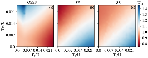
IV.2 Influence of DIT processes on the MIT of OSSF and SF phases
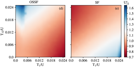
Here, we examine the effects of the DIT processes on the usual MIT of OSSF and SF phases, when the NN interactions are absent. For this, we numerically obtain the immiscibility condition in terms of inter-component onsite interaction strength as the intra and inter-component DIT strengths, and , are varied. That is, we investigate the MIT criterion as in Eq. (9) in the presence of DIT processes. The inter-component interaction strengths are fixed at . Then, we find the required strength of for the components to be immiscible ( becomes zero), which we denote as . We illustrate the variation of in the heatmaps shown in Fig. 3(d) and Fig. 3(e) for the OSSF and SF phases, respectively. To explore the condition in the OSSF phase [see Fig. 3(d)], we choose the chemical potential and hopping strength . For , we recover the known immiscibility condition . We observe that is decreased with the increase in for fixed , while it increases with the increase in for fixed . On the other hand, in the SF phase, the immiscibility condition gets modified in opposite way [see Fig. 3(e)]. The corresponding heatmap is obtained for and . We observe that is decreased (increased) with the increase (decrease) in (). Additionally, in both the cases for . These observations demonstrate that the MIT gets significantly influenced by the DIT processes. Furthermore, intra-component DIT processes favour immiscibility by lowering the value in the OSSF phase, whereas they favour miscibility in the SF phase. This opposite trend of in Fig. 3(d) and Fig. 3(e) is consistent with the observations made in Fig. 2 and the arguments presented in Sec.III.
Note that, so far we have considered fixed hopping strengths. This allows us to explore the MIT in the targeted quantum phases. But, we also extend our study for other values of the hopping strengths in Appendix. B. With the change in hopping strengths, the model is expected to show transitions between the OSSF, MI and SF phases. Therefore, we can probe the influence of DIT processes on the MIT of these phases.
IV.3 Phase diagram of two component BHM with DIT and NN interactions
We discuss the phase diagrams of the BHM in the presence of both DIT processes and NN interactions, which are presented in Fig. 4 (a) - (c) for three different values of . Similar to the previous case, the scale is fixed by . We consider and for the phase diagrams. For this weak value of the NN interaction strengths, the phase diagram remains qualitatively similar to that of the Fig. 3, that is, the parameter domains of the compressible phases surround the lobes of incompressible phases. However, the considered NN interaction strength is sufficient to withstand the quantum phases with checkerboard ordering in the density distribution, thereby stabilizing the DW and SS phases. Then, the phase diagram has parameter domains for the two-component DW and SS phases in addition to the MI and SF phases. For , we obtain the lobes of DW(2,0), MI(2), DW(2,4), MI(4), and so on, with increasing [see Fig. 4 (a)]. Here, we have adapted the bipartite lattice notation (discussed in Sec.II.3) with belonging to the two sub-lattices to mark the DW lobes. Note that these lobes are of incompressible phases with two-component filling equals to , , , and . The lobes for integer and half-integer filling are for MI and DW phases, respectively. The parameter domains of the SS phase envelope the DW(2,0) and DW(2,4) lobes, and its phase boundary is marked by the solid green line. Similar to Fig. 3, the phase diagram has the parameter domain of the OSSF phase to the left of the lobes of the incompressible phases. In this case, we additionally obtain parameter domains of the OSSS phase which is stabilized by both the DIT processes and NN interactions.
With the increase of , like in the previous case, Mott lobes with half-integer filling [for example, MI(1) and MI(3)] emerge [see Fig. 4(b)]. Additionally, DW phases with quarter filling, such as, DW(1,0), DW(1,2), DW(2,3), etc., get stabilized. Note that these DW phases have two-component filling equals to , and , respectively. Like in the previous case the SS and OSSS phases have parameter domains enveloping the the DW phases. But, it is important to note that the parameter regime of SS and OSSS phases shrink with increasing , which is evident from the comparison between Figs. 4(a)-(c). This trend is consistent as increasing inter-component onsite interaction results in stabilizing the insulating phases against the compressible SS and OSSS phases. For , the parameter domains of these phases are marginally present [see Fig. 4(c)]. Therefore, it is essential to consider larger NN interaction strengths to analyze the MIT of the SS phase. In this case, the phase diagram has lobes of DW(1,0), MI(1), DW(1,2), MI(2), and DW(2,3), corresponding to incompressible phases with two-component filling equals to , , , and , respectively.
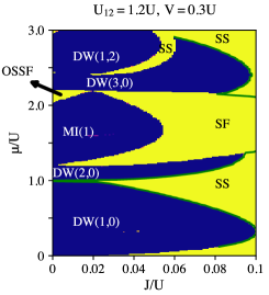
We now explore the phase diagram of the model with but keeping DIT strengths as previous. For such strong NN interaction strengths, we obtain larger parameter domain of the SS phase. Since with increasing the parameter region of the SS phase shrinks, an observation mentioned in the previous paragraph, here we present the phase diagram only for for brevity. In contrast to the case considered earlier, it is important to note that the stronger NN interactions significantly change the phase diagram, which is shown in Fig. 5. We notice enhanced usual lobes of DW(1,0), MI(1) and DW(1,2), in comparison to the Fig. 4(c). Additionally, deformed parameter domains of DW(2,0) and DW(3,0) are obtained next to MI(1) and DW(1,2). Note MI(1) and DW(2,0) phases have same two-component filling equals to . Similarly, filling of the DW(1,2) and DW(3,0) phases is . Therefore, the strong NN interaction results in additional DW phases. Interestingly, the transitions from MI(1) to DW(2,0) and DW(1,2) to DW(3,0) are intervened by the the parameter domains SF and SS phases, respectively. Similar to previous case, the SS phase appears next to the DW phases. However, it is important to note that we obtain significantly large parameter domain of the SS phase in contrast to the Fig. 4(c). Therefore, we can examine the influence of the DIT processes on the MIT transition in the two-component SS phase by making appropriate choice of the parameters. Furthermore, we also observe a small domain of the OSSF phase next to the left side of the MI(1) lobe.
IV.4 Influence of DIT processes on the MIT of OSSF, SF and SS phases
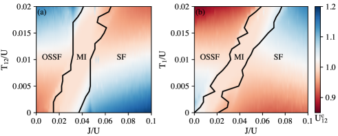
We now explore the effects of the DIT processes on the MIT transition of the OSSF, SF, and SS phases when the NN interactions are considered in the model. We consider the while examining the immiscibility condition for the OSSF and SF phases, whereas it is fixed to for the SS phase. Like earlier, we find the the required inter-component interaction strength, , for the immiscibility () as and are varied. The corresponding heatmaps are depicted in Fig. 6. We consider and for the OSSF phase [see Fig. 6(a)] and and for the SF phase [see Fig. 6(b)]. We observe qualitatively similar behaviour of as in Figs. 3(d) and (e). Thus, the immiscibility is favoured by the intra-component DIT processes in the OSSF phase. On the other hand, the dependence of in the SS phase [see Fig. 6(c)] is similar as in the SF phase. That is, decreases as we increase keeping fixed, whereas it increases as we increase keeping fixed. Thus, in the SF and SS phases, the immiscibility is favoured by inter-component DIT processes. Guided by the phase diagram presented in Fig. 5, we consider and to explore the effects of the DIT processes on MIT in the SS phase. This ensures that the two-component SS phase is always retained as the is varied to obtain the .
V Summary and discussion
In summary, we have theoretically investigated the MIT of a two-component bosonic mixture in the strongly interacting regime. Our study reveals that the MIT can be steered by controlling the DIT processes and NN interactions, when the mixture is tuned close to the immiscibility with respect to onsite interactions. We particularly study the MIT in the two-component OSSF, SF and SS phases, which are compressible quantum phases of the BHM model with DIT and NN interaction terms. Our investigation suggests as the immiscibility condition in the SF and SS phases, which is similar to the immiscibility condition in terms of onsite interaction strengths. In striking contrast, we obtain as the immiscibility condition for the OSSF phase. This characteristic arises due to the phase staggering of the OSSF phase. On the other hand, in all these phases the immiscibility condition is found to be when the MIT is driven with respect to the NN interactions.
Next, we have demonstrated that the DIT can significantly influence the MIT of the quantum phases in strongly interacting regime. For this we have analyzed the required inter-component interaction strength for immiscibility of the two components, . Our numerical analysis reveals that is considerably lowered or enhanced in the presence of DIT processes. Consistent with the above conclusion, we find that intra-component DIT processes favour immiscibility by lowering the value of in the OSSF phase. Whereas, miscibility is favoured by the inter-component DIT process, since is increased with the increase of for fixed . We obtain the opposite dependence of on the intra and inter-component DIT processes in the SF and SS phases. Here, the value of is significantly lowered with the increase in , implying the inter-component DIT processes favour immiscibility of the components. We have first obtained this dependence in the absence of NN interactions, which we latter corroborate to the case for finite NN interaction strengths. We obtain qualitatively analogous trend in both these cases. Furthermore, we present mean-field phase diagrams of the two-component BHM with the DIT and NN interaction terms.
Interaction induced processes are known to influence several equilibrium and dynamical properties of optical lattice systems in the strongly interacting regime. In this regime, the DIT can arise from strong onsite interaction or due to long-range interaction between the particles. Whereas, the NN interaction becomes relevant in long-range interacting systems. Therefore, the strengths of these processes can be tuned by changing the relevant interaction strength. In an optical lattice system with neutral atoms, the DIT strength can be varied by changing the scattering length for onsite interaction through Feshbach resonances Chin et al. (2010). In this case, the DIT can be tuned to same order of usual hopping process Meinert et al. (2013); Jürgensen et al. (2014). On the other hand, atoms or molecules having large dipole moments can interact additionally through long-range dipole-dipole interaction Sowiński et al. (2012); Baier et al. (2016); Reichsöllner et al. (2017). This not only contributes to the onsite interaction, but also gives rise to DIT processes and NN interactions Sowiński et al. (2012); Baier et al. (2016). The strength of dipole-dipole interaction between the constituent particles, can be controlled by tilting the polarization axis of the dipoles with respect to lattice plane Baier et al. (2016); Bandyopadhyay et al. (2019) or by rapidly rotating the polarization axis Giovanazzi et al. (2002); Tang et al. (2018). Consequently, strengths of the DIT process and NN interaction can be tuned. Recently, the DIT has also been observed in a minimal set of three Rydberg atoms using dipolar exchange interactions, where DIT occurs from the second order virtual hopping process Lienhard et al. (2020). Effects of the DIT process on the usual MI-SF transition has been demonstrated in optical lattice system with neutral Mark et al. (2011); Jürgensen et al. (2014) and magnetic atoms Baier et al. (2016). Additionally, influence of the DIT on quantum criticality of an effective Ising model has been studied in an optical lattice system with neutral atoms Meinert et al. (2013).
Our study concludes that the MIT of a two-component system can be influenced significantly by the DIT processes. Due to the high degree of control on tuning the strengths of the DIT and NN interactions, as discussed above, our findings can be probed in future experiments on optical lattice loaded with mixture of ultracold atoms.
Acknowledgements.
We gratefully acknowledge useful discussions with Philipp Hauke. R.B. acknowledges International Institute of Information Technology Hyderabad for kind hospitality during the progress of this work. S.B. acknowledges funding by the European Union under NextGenerationEU Prot. n. 2022ATM8FY (CUP: E53D23002240006), European Research Council (ERC) under the European Union’s Horizon 2020 research and innovation programme (grant agreement No 804305), Provincia Autonoma di Trento, QTN, the joint lab between University of Trento, FBK-Fondazione Bruno Kessler, INFN-National Institute for Nuclear Physics and CNR-National Research Council. Views and opinions expressed are however those of the author(s) only and do not necessarily reflect those of the European Union or European Commission. Neither the European Union nor the granting authority can be held responsible for them. S.B. acknowledges CINECA for the use of HPC resources under ISCRA-C projects ISSYK-2 (HP10CP8XXF) and DISYK (HP10CGNZG9).Appendix A Single Site Hamiltonian and mean-field energy
Here, we explicitly present the single site mean-field Hamiltonian in Eq.(3) for a 2D square lattice system. In 2D, a lattice index can be written as . The coordination number of a square lattice is , and the NN sites can have index . By adapting a notation , the individual terms of the Hamiltonian of the th site can be written as
| (10) | |||||
where, the mean-fields , , , and , are given in Eqs. (5) and (6). Then, we can cast the single-site mean-field energy function in terms of these mean-fields as . Here the energy due to hopping of the particles is
| (11) |
The onsite interaction energy is given by
Furthermore, the energy arising from the DIT processes is
and the NN interaction energy is
| (14) |
Note that, for the quantum phases having checkerboard distribution, the single-site mean-field energy can be expressed using the sub-lattice description. In addition, we can drop the complex conjugation notation (the asterisk symbol) to the order parameters. We have explained both these aspects in the main text (see Secs.II.1 and II.3). Therefore, we can write the mean-field energy contributions of a site as
and
| (16) |
due to the DIT processes and NN interactions, respectively.
Appendix B Influence of DIT processes on the MIT (varying )
Here, we extend our study on the dependence of the immiscibility condition by varying hopping strength , and keeping chemical potential fixed. As discussed earlier, critical value of for MIT depends on the inter and intra-component DIT processes for a fixed value of chemical potential and hopping strength in the phase diagram. To extend our results for larger parameter domain of the phase diagram, we vary the hopping strength for a fixed value of chemical potential, and we compute . In the Fig. 7 (a), we show the heatmap of of MIT for chemical potential , intra-component DIT, . As we increase hopping strength, we encounter three quantum phases OSSF, MI and SF. For the OSSF phase, we observe the enhancement in as we increase . While in the SF phase, we observe decreases as we increase . The black line in Fig. 7 marks the OSSF-MI and MI-SF phase boundaries. In Fig. 7 (b), we show the heatmap for by fixing the inter-component DIT strength, . We now vary the for a fixed value. Like earlier, we enter in the OSSF, MI and SF phases as we vary hopping strengths. The critical value of for MIT shows opposite trend compared to Fig. 7 (a). The critical value of decreases as we increase in the OSSF phase, while it increases in the SF phase. We emphasize that the observations are consistent with the results reported in the main text.
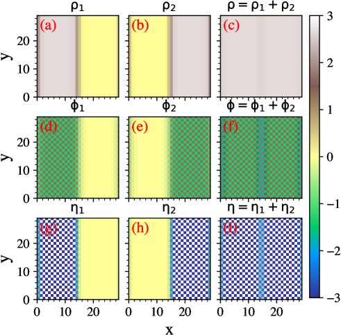
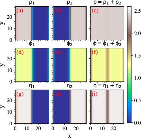
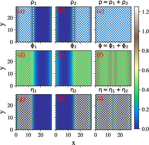
Appendix C Distributions of density and order parameters in the immiscible phase
Here, we present the density distributions of the immiscible phase in the OSSF, SF and SS phase. To be specific, we show the side by side density distribution in these phases. For the OSSF phase of BHM, we consider , and , and show the immiscible density distribution in the Fig. 8 (a-c). In the Fig. 8 (d-f), we show the corresponding SF order parameter and in Fig. 8 (g-i) we show the corresponding density transport parameter . The SF order parameter and density transport parameter show sign staggering between adjacent site and forms a checkerboard pattern. Further, we observe the side by side density distributions in the SF and SS phase shown in Fig. 9 and 10 respectively. For the SF phase, as mentioned earlier, the SF order parameter, density transport parameter and average density at each site is uniform. While in the SS phase, we observe that average density, SF order parameter and density transport parameter have checkerboard pattern. The numerical parameters for SF phase are , and . We set the NN interactions to be zero for both OSSF and SF phase. While for SS phase we consider , and .
References
- Sabbatini et al. (2011) J. Sabbatini, W. H. Zurek, and M. J. Davis, Phys. Rev. Lett. 107, 230402 (2011).
- Hall et al. (1998) D. S. Hall, M. R. Matthews, J. R. Ensher, C. E. Wieman, and E. A. Cornell, Phys. Rev. Lett. 81, 1539 (1998).
- Mertes et al. (2007) K. M. Mertes, J. W. Merrill, R. Carretero-González, D. J. Frantzeskakis, P. G. Kevrekidis, and D. S. Hall, Phys. Rev. Lett. 99, 190402 (2007).
- Papp et al. (2008) S. B. Papp, J. M. Pino, and C. E. Wieman, Phys. Rev. Lett. 101, 040402 (2008).
- Tojo et al. (2010) S. Tojo, Y. Taguchi, Y. Masuyama, T. Hayashi, H. Saito, and T. Hirano, Phys. Rev. A 82, 033609 (2010).
- McCarron et al. (2011) D. J. McCarron, H. W. Cho, D. L. Jenkin, M. P. Köppinger, and S. L. Cornish, Phys. Rev. A 84, 011603 (2011).
- Wacker et al. (2015) L. Wacker, N. B. Jørgensen, D. Birkmose, R. Horchani, W. Ertmer, C. Klempt, N. Winter, J. Sherson, and J. J. Arlt, Phys. Rev. A 92, 053602 (2015).
- Wang et al. (2016) F. Wang, X. Li, D. Xiong, and D. Wang, J. Phys. B 49, 015302 (2016).
- Eto et al. (2016) Y. Eto, M. Takahashi, M. Kunimi, H. Saito, and T. Hirano, New J. Phys. 18, 073029 (2016).
- Modugno et al. (2001) G. Modugno, G. Ferrari, G. Roati, R. J. Brecha, A. Simoni, and M. Inguscio, Science 294, 1320 (2001).
- Modugno et al. (2002) G. Modugno, M. Modugno, F. Riboli, G. Roati, and M. Inguscio, Phys. Rev. Lett. 89, 190404 (2002).
- Lercher et al. (2011) A. Lercher, T. Takekoshi, M. Debatin, B. Schuster, R. Rameshan, F. Ferlaino, R. Grimm, and H.-C. Nägerl, Eur. Phys. J. D 65, 3 (2011).
- Pasquiou et al. (2013) B. Pasquiou, A. Bayerle, S. M. Tzanova, S. Stellmer, J. Szczepkowski, M. Parigger, R. Grimm, and F. Schreck, Phys. Rev. A 88, 023601 (2013).
- Cavicchioli et al. (2022) L. Cavicchioli, C. Fort, M. Modugno, F. Minardi, and A. Burchianti, Phys. Rev. Res. 4, 043068 (2022).
- Myatt et al. (1997) C. J. Myatt, E. A. Burt, R. W. Ghrist, E. A. Cornell, and C. E. Wieman, Phys. Rev. Lett. 78, 586 (1997).
- Stamper-Kurn et al. (1998) D. M. Stamper-Kurn, M. R. Andrews, A. P. Chikkatur, S. Inouye, H.-J. Miesner, J. Stenger, and W. Ketterle, Phys. Rev. Lett. 80, 2027 (1998).
- Stenger et al. (1998) J. Stenger, S. Inouye, D. M. Stamper-Kurn, H.-J. Miesner, A. P. Chikkatur, and W. Ketterle, Nature (London) 396, 345 (1998).
- Maddaloni et al. (2000) P. Maddaloni, M. Modugno, C. Fort, F. Minardi, and M. Inguscio, Phys. Rev. Lett. 85, 2413 (2000).
- Delannoy et al. (2001) G. Delannoy, S. G. Murdoch, V. Boyer, V. Josse, P. Bouyer, and A. Aspect, Phys. Rev. A 63, 051602 (2001).
- Sadler et al. (2006) L. E. Sadler, J. M. Higbie, S. R. Leslie, M. Vengalattore, and D. M. Stamper-Kurn, Nature (London) 443, 312 (2006).
- Anderson et al. (2009) R. P. Anderson, C. Ticknor, A. I. Sidorov, and B. V. Hall, Phys. Rev. A 80, 023603 (2009).
- Fava et al. (2018) E. Fava, T. Bienaimé, C. Mordini, G. Colzi, C. Qu, S. Stringari, G. Lamporesi, and G. Ferrari, Phys. Rev. Lett. 120, 170401 (2018).
- Farolfi et al. (2020) A. Farolfi, D. Trypogeorgos, C. Mordini, G. Lamporesi, and G. Ferrari, Phys. Rev. Lett. 125, 030401 (2020).
- Farolfi et al. (2021) A. Farolfi, A. Zenesini, D. Trypogeorgos, C. Mordini, A. Gallemí, A. Roy, A. Recati, G. Lamporesi, and G. Ferrari, Nature Physics 17, 1359 (2021).
- Cominotti et al. (2022) R. Cominotti, A. Berti, A. Farolfi, A. Zenesini, G. Lamporesi, I. Carusotto, A. Recati, and G. Ferrari, Phys. Rev. Lett. 128, 210401 (2022).
- Händel et al. (2011) S. Händel, T. P. Wiles, A. L. Marchant, S. A. Hopkins, C. S. Adams, and S. L. Cornish, Phys. Rev. A 83, 053633 (2011).
- Sugawa et al. (2011) S. Sugawa, R. Yamazaki, S. Taie, and Y. Takahashi, Phys. Rev. A 84, 011610 (2011).
- Ferrier-Barbut et al. (2014) I. Ferrier-Barbut, M. Delehaye, S. Laurent, A. T. Grier, M. Pierce, B. S. Rem, F. Chevy, and C. Salomon, Science 345, 1035 (2014).
- DeSalvo et al. (2017) B. J. DeSalvo, K. Patel, J. Johansen, and C. Chin, Phys. Rev. Lett. 119, 233401 (2017).
- DeSalvo et al. (2019) B. J. DeSalvo, K. Patel, G. Cai, and C. Chin, Nature 568, 61 (2019).
- Gautam and Angom (2010) S. Gautam and D. Angom, J. Phys. B 43, 095302 (2010).
- Gautam and Angom (2011) S. Gautam and D. Angom, J. Phys. B 44, 025302 (2011).
- Pattinson et al. (2013) R. W. Pattinson, T. P. Billam, S. A. Gardiner, D. J. McCarron, H. W. Cho, S. L. Cornish, N. G. Parker, and N. P. Proukakis, Phys. Rev. A 87, 013625 (2013).
- Lee et al. (2016) K. L. Lee, N. B. Jørgensen, I.-K. Liu, L. Wacker, J. J. Arlt, and N. P. Proukakis, Phys. Rev. A 94, 013602 (2016).
- Wen et al. (2020) L. Wen, H. Guo, Y.-J. Wang, A.-Y. Hu, H. Saito, C.-Q. Dai, and X.-F. Zhang, Phys. Rev. A 101, 033610 (2020).
- Nho and Landau (2007) K. Nho and D. P. Landau, Phys. Rev. A 76, 053610 (2007).
- Roy et al. (2014) A. Roy, S. Gautam, and D. Angom, Phys. Rev. A 89, 013617 (2014).
- Roy and Angom (2015) A. Roy and D. Angom, Phys. Rev. A 92, 011601 (2015).
- Suthar and Angom (2017) K. Suthar and D. Angom, Phys. Rev. A 95, 043602 (2017).
- Ota et al. (2019) M. Ota, S. Giorgini, and S. Stringari, Phys. Rev. Lett. 123, 075301 (2019).
- Roy et al. (2021) A. Roy, M. Ota, A. Recati, and F. Dalfovo, Phys. Rev. Res. 3, 013161 (2021).
- Spada et al. (2023) G. Spada, L. Parisi, G. Pascual, N. G. Parker, T. P. Billam, S. Pilati, J. Boronat, and S. Giorgini, SciPost Phys. 15, 171 (2023).
- Bandyopadhyay et al. (2017) S. Bandyopadhyay, A. Roy, and D. Angom, Phys. Rev. A 96, 043603 (2017).
- Kuopanportti et al. (2019) P. Kuopanportti, S. Bandyopadhyay, A. Roy, and D. Angom, Phys. Rev. A 100, 033615 (2019).
- Ao and Chui (1998) P. Ao and S. T. Chui, Phys. Rev. A 58, 4836 (1998).
- Timmermans (1998) E. Timmermans, Phys. Rev. Lett. 81, 5718 (1998).
- Pu and Bigelow (1998) H. Pu and N. P. Bigelow, Phys. Rev. Lett. 80, 1130 (1998).
- Ho and Shenoy (1996) T.-L. Ho and V. B. Shenoy, Phys. Rev. Lett. 77, 3276 (1996).
- Pethick and Smith (2002) C. J. Pethick and H. Smith, Bose-Einstein condensation in Dilute Gases (Cambridge University Press (New York), 2002).
- Morsch and Oberthaler (2006) O. Morsch and M. Oberthaler, Rev. Mod. Phys. 78, 179 (2006).
- Bloch et al. (2008) I. Bloch, J. Dalibard, and W. Zwerger, Rev. Mod. Phys. 80, 885 (2008).
- Lewenstein et al. (2012) M. Lewenstein, A. Sanpera, and V. Ahufinger, Ultracold Atoms in Optical Lattices: Simulating quantum many-body systems (Oxford University Press, 2012).
- Gross and Bloch (2017) C. Gross and I. Bloch, Science 357, 995 (2017).
- Mazzarella et al. (2006) G. Mazzarella, S. M. Giampaolo, and F. Illuminati, Phys. Rev. A 73, 013625 (2006).
- Dutta et al. (2015) O. Dutta, M. Gajda, P. Hauke, M. Lewenstein, D.-S. Lühmann, B. A. Malomed, T. Sowiński, and J. Zakrzewski, Rep. Prog. Phys. 78, 066001 (2015).
- Bloch et al. (2012) I. Bloch, J. Dalibard, and S. Nascimbène, Nature Physics 8, 267 (2012).
- Yang et al. (2020a) B. Yang, H. Sun, R. Ott, H.-Y. Wang, T. V. Zache, J. C. Halimeh, Z.-S. Yuan, P. Hauke, and J.-W. Pan, Nature 587, 392 (2020a).
- Yang et al. (2020b) B. Yang, H. Sun, C.-J. Huang, H.-Y. Wang, Y. Deng, H.-N. Dai, Z.-S. Yuan, and J.-W. Pan, Science 369, 550 (2020b).
- Ebadi et al. (2021) S. Ebadi, T. T. Wang, H. Levine, A. Keesling, G. Semeghini, A. Omran, D. Bluvstein, R. Samajdar, H. Pichler, W. W. Ho, S. Choi, S. Sachdev, M. Greiner, V. Vuletić, and M. D. Lukin, Nature 595, 227 (2021).
- Bakr et al. (2009) W. S. Bakr, J. I. Gillen, A. Peng, S. Fölling, and M. Greiner, Nature 462, 74 (2009).
- Kuhr (2016) S. Kuhr, National Science Review 3, 170 (2016).
- Jaksch and Zoller (2005) D. Jaksch and P. Zoller, Annals of Physics 315, 52 (2005), special Issue.
- Lewenstein et al. (2007) M. Lewenstein, A. Sanpera, V. Ahufinger, B. Damski, A. Sen(De), and U. Sen, Adv. Phys. 56, 243 (2007).
- Zhang et al. (2018) D.-W. Zhang, Y.-Q. Zhu, Y. X. Zhao, H. Yan, and S.-L. Zhu, Advances in Physics 67, 253 (2018).
- Hofstetter and Qin (2018) W. Hofstetter and T. Qin, J. Phys. B 51, 082001 (2018).
- Tarruell and Sanchez-Palencia (2018) L. Tarruell and L. Sanchez-Palencia, Comptes Rendus Physique 19, 365 (2018).
- Wiese (2013) U.-J. Wiese, Annalen der Physik 525, 777 (2013).
- Aidelsburger et al. (2022) M. Aidelsburger et al., Phil. Trans. R. Soc. A 380, 20210064 (2022).
- Zohar et al. (2015) E. Zohar, J. I. Cirac, and B. Reznik, Rep. Prog. Phys. 79, 014401 (2015).
- Halimeh et al. (2023) J. C. Halimeh, M. Aidelsburger, F. Grusdt, P. Hauke, and B. Yang, (2023), arXiv:2310.12201 .
- Monroe (2002) C. Monroe, Nature 416, 238 (2002).
- Jaksch (2004) D. Jaksch, Contemp. Phys. 45, 367 (2004).
- García-Ripoll et al. (2005) J. J. García-Ripoll, P. Zoller, and J. I. Cirac, J. Phys. B 38, S567 (2005).
- Gezerlis and Carlson (2008) A. Gezerlis and J. Carlson, Phys. Rev. C 77, 032801 (2008).
- Strinati et al. (2018) G. C. Strinati, P. Pieri, G. Röpke, P. Schuck, and M. Urban, Phys. Rep. 738, 1 (2018).
- Hung et al. (2013) C.-L. Hung, V. Gurarie, and C. Chin, Science 341, 1213 (2013).
- Schmiedmayer and Berges (2013) J. Schmiedmayer and J. Berges, Science 341, 1188 (2013).
- Chatrchyan et al. (2021) A. Chatrchyan, K. T. Geier, M. K. Oberthaler, J. Berges, and P. Hauke, Phys. Rev. A 104, 023302 (2021).
- Wei and Sedrakyan (2021) C. Wei and T. A. Sedrakyan, Phys. Rev. A 103, 013323 (2021).
- Uhrich et al. (2023) P. Uhrich, S. Bandyopadhyay, N. Sauerwein, J. Sonner, J.-P. Brantut, and P. Hauke, (2023), arXiv:2303.11343 .
- Hubbard (1963) J. Hubbard, Proc. Royal Soc. A 276, 238 (1963).
- Fisher et al. (1989) M. P. A. Fisher, P. B. Weichman, G. Grinstein, and D. S. Fisher, Phys. Rev. B 40, 546 (1989).
- Jaksch et al. (1998) D. Jaksch, C. Bruder, J. I. Cirac, C. W. Gardiner, and P. Zoller, Phys. Rev. Lett. 81, 3108 (1998).
- Greiner et al. (2002) M. Greiner, O. Mandel, T. Esslinger, T. W. Hänsch, and I. Bloch, Nature (London) 415, 39 (2002).
- Bakr et al. (2010) W. S. Bakr, A. Peng, M. E. Tai, R. Ma, J. Simon, J. I. Gillen, S. Fölling, L. Pollet, and M. Greiner, Science 329, 547 (2010).
- Sowiński et al. (2012) T. Sowiński, O. Dutta, P. Hauke, L. Tagliacozzo, and M. Lewenstein, Phys. Rev. Lett. 108, 115301 (2012).
- Lühmann et al. (2012) D.-S. Lühmann, O. Jürgensen, and K. Sengstock, New J. Phys. 14, 033021 (2012).
- Jürgensen et al. (2012) O. Jürgensen, K. Sengstock, and D.-S. Lühmann, Phys. Rev. A 86, 043623 (2012).
- Maik et al. (2013) M. Maik, P. Hauke, O. Dutta, M. Lewenstein, and J. Zakrzewski, New J. Phys. 15, 113041 (2013).
- Jürgensen et al. (2014) O. Jürgensen, F. Meinert, M. J. Mark, H.-C. Nägerl, and D.-S. Lühmann, Phys. Rev. Lett. 113, 193003 (2014).
- Jürgensen et al. (2015) O. Jürgensen, K. Sengstock, and D.-S. Lühmann, Scientific Reports 5, 12912 (2015).
- Lühmann (2016) D.-S. Lühmann, Phys. Rev. A 94, 011603 (2016).
- Sengupta et al. (2005) P. Sengupta, L. P. Pryadko, F. Alet, M. Troyer, and G. Schmid, Phys. Rev. Lett. 94, 207202 (2005).
- Scarola and Das Sarma (2005) V. W. Scarola and S. Das Sarma, Phys. Rev. Lett. 95, 033003 (2005).
- Ng and Chen (2008) K.-K. Ng and Y.-C. Chen, Phys. Rev. B 77, 052506 (2008).
- Iskin (2011) M. Iskin, Phys. Rev. A 83, 051606 (2011).
- Suthar et al. (2020a) K. Suthar, H. Sable, R. Bai, S. Bandyopadhyay, S. Pal, and D. Angom, Phys. Rev. A 102, 013320 (2020a).
- Johnstone et al. (2019) D. Johnstone, N. Westerberg, C. W. Duncan, and P. Öhberg, Phys. Rev. A 100, 043614 (2019).
- Suthar et al. (2020b) K. Suthar, R. Kraus, H. Sable, D. Angom, G. Morigi, and J. Zakrzewski, Phys. Rev. B 102, 214503 (2020b).
- Suthar and Ng (2022) K. Suthar and K.-K. Ng, Phys. Rev. A 106, 063313 (2022).
- Baier et al. (2016) S. Baier, M. J. Mark, D. Petter, K. Aikawa, L. Chomaz, Z. Cai, M. Baranov, P. Zoller, and F. Ferlaino, Science 352, 201 (2016).
- Chowdhury et al. (2022) D. Chowdhury, A. Georges, O. Parcollet, and S. Sachdev, Rev. Mod. Phys. 94, 035004 (2022).
- Bandyopadhyay et al. (2023) S. Bandyopadhyay, P. Uhrich, A. Paviglianiti, and P. Hauke, Quantum 7, 1022 (2023).
- Panchenko (2015) D. Panchenko, The Sherrington-Kirkpatrick Model (Springer New York, NY, 2015).
- Lechner et al. (2015) W. Lechner, P. Hauke, and P. Zoller, Science Advances 1, e1500838 (2015).
- Pu et al. (2001) H. Pu, W. Zhang, and P. Meystre, Phys. Rev. Lett. 87, 140405 (2001).
- de Paz et al. (2013) A. de Paz, A. Sharma, A. Chotia, E. Maréchal, J. H. Huckans, P. Pedri, L. Santos, O. Gorceix, L. Vernac, and B. Laburthe-Tolra, Phys. Rev. Lett. 111, 185305 (2013).
- Góral et al. (2002) K. Góral, L. Santos, and M. Lewenstein, Phys. Rev. Lett. 88, 170406 (2002).
- Danshita and Sá de Melo (2009) I. Danshita and C. A. R. Sá de Melo, Phys. Rev. Lett. 103, 225301 (2009).
- Capogrosso-Sansone et al. (2010) B. Capogrosso-Sansone, C. Trefzger, M. Lewenstein, P. Zoller, and G. Pupillo, Phys. Rev. Lett. 104, 125301 (2010).
- Bandyopadhyay et al. (2019) S. Bandyopadhyay, R. Bai, S. Pal, K. Suthar, R. Nath, and D. Angom, Phys. Rev. A 100, 053623 (2019).
- Reichsöllner et al. (2017) L. Reichsöllner, A. Schindewolf, T. Takekoshi, R. Grimm, and H.-C. Nägerl, Phys. Rev. Lett. 118, 073201 (2017).
- Kuklov and Svistunov (2003) A. B. Kuklov and B. V. Svistunov, Phys. Rev. Lett. 90, 100401 (2003).
- Kuklov et al. (2004) A. Kuklov, N. Prokof’ev, and B. Svistunov, Phys. Rev. Lett. 92, 050402 (2004).
- Isacsson et al. (2005) A. Isacsson, M.-C. Cha, K. Sengupta, and S. M. Girvin, Phys. Rev. B 72, 184507 (2005).
- Bai et al. (2020) R. Bai, D. Gaur, H. Sable, S. Bandyopadhyay, K. Suthar, and D. Angom, Phys. Rev. A 102, 043309 (2020).
- Altman et al. (2003) E. Altman, W. Hofstetter, E. Demler, and M. D. Lukin, New J. Phys. 5, 113 (2003).
- Morera et al. (2019) I. Morera, A. Polls, and B. Juliá-Díaz, Scientific Reports 9, 9424 (2019).
- Dutta et al. (2011) O. Dutta, A. Eckardt, P. Hauke, B. Malomed, and M. Lewenstein, New J. Phys. 13, 023019 (2011).
- Soltan-Panahi et al. (2012) P. Soltan-Panahi, D.-S. Lühmann, J. Struck, P. Windpassinger, and K. Sengstock, Nature Physics 8, 71 (2012).
- Bandyopadhyay et al. (2022) S. Bandyopadhyay, H. Sable, D. Gaur, R. Bai, S. Mukerjee, and D. Angom, Phys. Rev. A 106, 043301 (2022).
- Kühner et al. (2000) T. D. Kühner, S. R. White, and H. Monien, Phys. Rev. B 61, 12474 (2000).
- Trautmann et al. (2018) A. Trautmann, P. Ilzhöfer, G. Durastante, C. Politi, M. Sohmen, M. J. Mark, and F. Ferlaino, Phys. Rev. Lett. 121, 213601 (2018).
- Rokhsar and Kotliar (1991) D. S. Rokhsar and B. G. Kotliar, Phys. Rev. B 44, 10328 (1991).
- Sheshadri et al. (1993) K. Sheshadri, H. R. Krishnamurthy, R. Pandit, and T. V. Ramakrishnan, EPL 22, 257 (1993).
- Anufriiev and Zaleski (2016) S. Anufriiev and T. A. Zaleski, Phys. Rev. A 94, 043613 (2016).
- Bai et al. (2018) R. Bai, S. Bandyopadhyay, S. Pal, K. Suthar, and D. Angom, Phys. Rev. A 98, 023606 (2018).
- Ş G Söyler et al. (2009) Ş G Söyler, B. Capogrosso-Sansone, N. V. Prokof’ev, and B. V. Svistunov, New J. Phys. 11, 073036 (2009).
- Chen and Wu (2003) G.-H. Chen and Y.-S. Wu, Phys. Rev. A 67, 013606 (2003).
- Roscilde and Cirac (2007) T. Roscilde and J. I. Cirac, Phys. Rev. Lett. 98, 190402 (2007).
- Buonsante et al. (2008) P. Buonsante, S. M. Giampaolo, F. Illuminati, V. Penna, and A. Vezzani, Phys. Rev. Lett. 100, 240402 (2008).
- Alon et al. (2006) O. E. Alon, A. I. Streltsov, and L. S. Cederbaum, Phys. Rev. Lett. 97, 230403 (2006).
- Mishra et al. (2007) T. Mishra, R. V. Pai, and B. P. Das, Phys. Rev. A 76, 013604 (2007).
- Zhan and McCulloch (2014) F. Zhan and I. P. McCulloch, Phys. Rev. A 89, 057601 (2014).
- Zhan et al. (2014) F. Zhan, J. Sabbatini, M. J. Davis, and I. P. McCulloch, Phys. Rev. A 90, 023630 (2014).
- Lingua et al. (2015) F. Lingua, M. Guglielmino, V. Penna, and B. Capogrosso Sansone, Phys. Rev. A 92, 053610 (2015).
- Shrestha (2010) U. Shrestha, Phys. Rev. A 82, 041603 (2010).
- Zheng et al. (2024) Y.-G. Zheng, A. Luo, Y.-C. Shen, M.-G. He, Z.-H. Zhu, Y. Liu, W.-Y. Zhang, H. Sun, Y. Deng, Z.-S. Yuan, and J.-W. Pan, (2024), arXiv:2403.03479 .
- Chin et al. (2010) C. Chin, R. Grimm, P. Julienne, and E. Tiesinga, Rev. Mod. Phys. 82, 1225 (2010).
- Meinert et al. (2013) F. Meinert, M. J. Mark, E. Kirilov, K. Lauber, P. Weinmann, A. J. Daley, and H.-C. Nägerl, Phys. Rev. Lett. 111, 053003 (2013).
- Giovanazzi et al. (2002) S. Giovanazzi, A. Görlitz, and T. Pfau, Phys. Rev. Lett. 89, 130401 (2002).
- Tang et al. (2018) Y. Tang, W. Kao, K.-Y. Li, and B. L. Lev, Phys. Rev. Lett. 120, 230401 (2018).
- Lienhard et al. (2020) V. Lienhard, P. Scholl, S. Weber, D. Barredo, S. de Léséleuc, R. Bai, N. Lang, M. Fleischhauer, H. P. Büchler, T. Lahaye, and A. Browaeys, Phys. Rev. X 10, 021031 (2020).
- Mark et al. (2011) M. J. Mark, E. Haller, K. Lauber, J. G. Danzl, A. J. Daley, and H.-C. Nägerl, Phys. Rev. Lett. 107, 175301 (2011).